NBER WORKING PAPER SERIES

SKI-LIFT PRICING, WITH ANAPPLICATION TO THE LABOR MARKET

Robert J. Barro

Paul M. Romer

Working Paper No. 1985

NATIONAL BUREAU OF ECONOMIC RESEARCH1050 Massachusetts Avenue

Cambridge, MA 02138July 1985

The research reported here is part of the NBERTs research programin Economic Fluctuations. Any opinions expressed are those of theauthors and not those of the National Bureau of Economic Research.

Working Paper #1985July 1986

Ski-Lift Pricing, with an Application to the Labor Market

ABSTRACT

The market for ski runs or amusement rides often features lump—sum

admission tickets with no explicit price per ride. Therefore, the equation

of the demand for rides to the supply involves queues, which are

systematically longer during peak periods, such as weekends. Moreover, the

prices of admission tickets are much less responsive than the length of

queues to variations in demand, even when these variations are predictable.

We show that this method of pricing generates nearly efficient outcomes under

plausible conditions. In particular, the existence of queues and the

"stickiness" of prices do not necessarily mean that rides are allocated

improperly or that firms choose inefficient levels of investment. We then

draw an analogy between "ski—lift pricing" and the use of profit-sharing

schemes in the labor market. Although firms face explicit marginal costs of

labor that are sticky and less than workers' reservation wages, and although

the pool of profits seems to create a common—property problem for workers,

this method of pricing can approximate the competitive outcomes for

employment and total labor compensation.

Robert J. Barro Paul M. RomerDepartment of Economics Department of EconomicsUniversity of Rochester University of RochesterRochester, NY 14627 Rochester, NY 14627

During Christmas or Spring vacation, most ski areas have long lines. The

same is true for Disneyland and other amusement parks in peak season. This

type of crowding does not depend on surprises in demand, but instead is

systematic. Most economists look at chronic queuing and conjecture that the

suppliers would do better by raising prices. Further, most economists would

argue that the failure to price properly leads to inefficient allocations of

rides, as well as improper investment decisions. But the regular occurrence

of lines in some markets suggests that it is economists, rather than suppliers

(who have survived), who are missing something.

We argue in this paper that competitive suppliers of ski-lift services

(amusement rides, etc.) may rationally set prices so that queues occur

regularly and are longer at peak times. Under plausible assumptions, this

method of pricing can support efficient allocative decisions. In equilibrium,

owners of ski areas set prices for all-day lift tickets (or equivalently, for

admission tickets to amusement parks) by maximizing profits subject to a

downward-sloping demand curve. Yet this appearance of monopoly power leads to

no inefficiency. Moreover, the equilibrium price charged for a lift ticket

may not rise with expansions of demand. Sticky prices may be consistent with

optimization by suppliers and with efficient choices of quantities.

The explanation for this last result is that skiers calculate the

effective price per lift ride by summing opportunity costs, transportation

costs and the price of an all-day lift ticket, and then dividing this sum by

the number of rides received. This effective price varies inversely with the

number of skiers, and thereby changes in the correct direction with

2

fluctuations in demand, even If the lift-ticket price is constant. Under

plausible conditions, the magnitude of response of the effective price is also

nearly "correct."

We go on to develop parallels between the ski-lift example and the labor

market. Fully flexible wages correspond to fully flexible prices per lift

ride. But, as In the case of skiing, it is possible to implement alternative

methods of pricing that support the efficient outcomes. We show as an example

that a profit-sharing scheme, such as that described in Weitzman (1985)

parallels the use of admission tickets. Further, under some conditions—and

without appealing to long-term contracts—there is little efficiency loss by

having sticky wages and fixed parameters of the profit-sharing formula.

In the ski-lift and labor-market examples, the contracts and trading

arrangements that agents use may depart significantly from the textbook

description of a competitive market. Stated prices may differ from marginal

values. Some agents may act explicitly as price setters facing finite

elasticities, while others may face explicit or implicit quantity constraints.

Without forcing a departure from these institutional conventions, competitive

forces may nonetheless induce efficient outcomes. To decide whether a market

is competitive or efficient, economists cannot accept at face value the

description offered by agents of how a market operates. The prices quoted In

actual contracts and trades may bear little relation to the theoretical

contructs that economists call competitive equilibrium prices.

2. The Suppy and Demand for Ski-Lift Services

We will show that the ski-area equilibrium with queues and sticky prices

for all-day lift tickets is essentially a repackaged or disguised version of a

3

conventional equilibrium with a price per lift ride that adjusts in the usual

fashion. To do this, we analyze the conventional equilibrium first. Section

2.1 describes the market for ski-lift rides and works out the equilibrium.

Section 2.2 then illustrates how the quantities and prices from this efficient

solution can be replicated in an equilibrium with lift-ticket pricing and

queues. Section 2.3 considers the factors that might influence the choice

between these two institutional arrangements for supporting the equilibrium.

Section 2.4 illustrates why lift-ticket prices may not respoñd to changes in

demand. The results in these four subsections are derived under the

assumption that all ski areas are identical and that individuals differ only

In a limited sense. Section 3 shows how the results are modified with more

interesting heterogeneity across consumers and producers. Then Section 4

shows how a parallel analysis applies to profit-sharing schemes in the labor

market.

2.1 Equilibrium with Ride Tickets

Consider a group of identical, competitive ski-lift operators, each of

whom sells ride tickets at a price P per ride. Each firm has a fixed capacity

and therefore supplies inelastically the total quantity of rides x.

Flexibility in this quantity at some positive marginal cost is more realistic,

since suppliers can open more lift lines or perhaps operate the existing ones

at greater speed. But these modifications would not change the nature of the

problem. In the present case the industry's total supply of rides is Jx,

where J is the fixed number of firms.

4

The demand for skiing involves first, the decision to participate—that

is, whether to go skiing—and second the quantity of rides to demand

contingent on participation. To abstract from income effects, suppose that

all individuals have common preferences that can be represented in the

quasi-linear form U(q) + z, where q is the number of lift rides, U is a

strictly concave utility function, and z is real expenditure on goods other

than skiing. For someone who chooses to ski, the expenditure on other goods

is z = Y - Pg - c, where Y is real income, Pq is the expenditure on lift

rides, and c is an individual specific, lump-sum cost of going skiing. It is

quasi-fixed in the sense that the cost for a non-skier is zero, but the cost

for a skier is Independent of the number of ski runs.

Since P is a price per ride, the quantity of rides demanded by those who

ski follows from the condition, U'(q,) = P. Inverting this equation, the

number of rides demanded per person appears as a usual demand curve with a

negative slope: q1 = D(P), with D'(P) < 0. Since we assume in this section

that U is the same for all individuals, each person who participates demands

the same number of rides, q. Section 3 generalizes the results to allow for

cross-sectional differences in the demand curves for ski-lift rides.

An Individual participates if the net (money value) of the utility

gained, U[D(P)] - P.D(P), exceeds the fixed cost c. In order to neglect

Integer constraints, we assume that the agents In the economy can be

represented as a continuum [0,M}, arranged In terms of Increasing costs of

participating. We also want to allow the cost for all Individuals to vary

over time. Thus we describe the costs In terms of a family of cost functions

c(j), which are continuous and strictly Increasing In agent type I and are

5

indexed by a shift parameter s. For example, during vacation periods, the

cost for each individual is shifted downward relative to that at other times.

Given a price P for lift rides, all individuals with a cost c(i) less than

the benefits from skiing, U{D(P)J - P'D(P), choose to participate. Thus, the

number of individuals N who choose to ski is given by

(1) N = N(P) = c1{U[D(P)J - P.D(P)).

By the strict concavity of U, the benefits from skiing fall with an increase

in the price per ride P, so the number of skiers falls as well. A downward

shift in the distribution of fixed costs (as on weekends) raises the value of

N for a given P.

By specifying that the ski areas are competitive, we mean that each is

small enough that its actions have a negligible impact on aggregate

quantities. In this model (though not in those that follow) competitive

behavior implies that firms take prices as given. Equilibrium requires that

the total capacity of rides, Jx, equal the total number demanded, qN—that is,

(2) Jx D(P).N(P) = D(P)•c1{U[D(P)J P.D(P)}

For a given value of Jx, this condition determines the equilibrium price per

ride P. As one would expect, the price P falls with an increase in total

capacity, Jx, and rises with an increase in the level of demand such as that

generated from a downward shift in the level of fixed costs c.

6

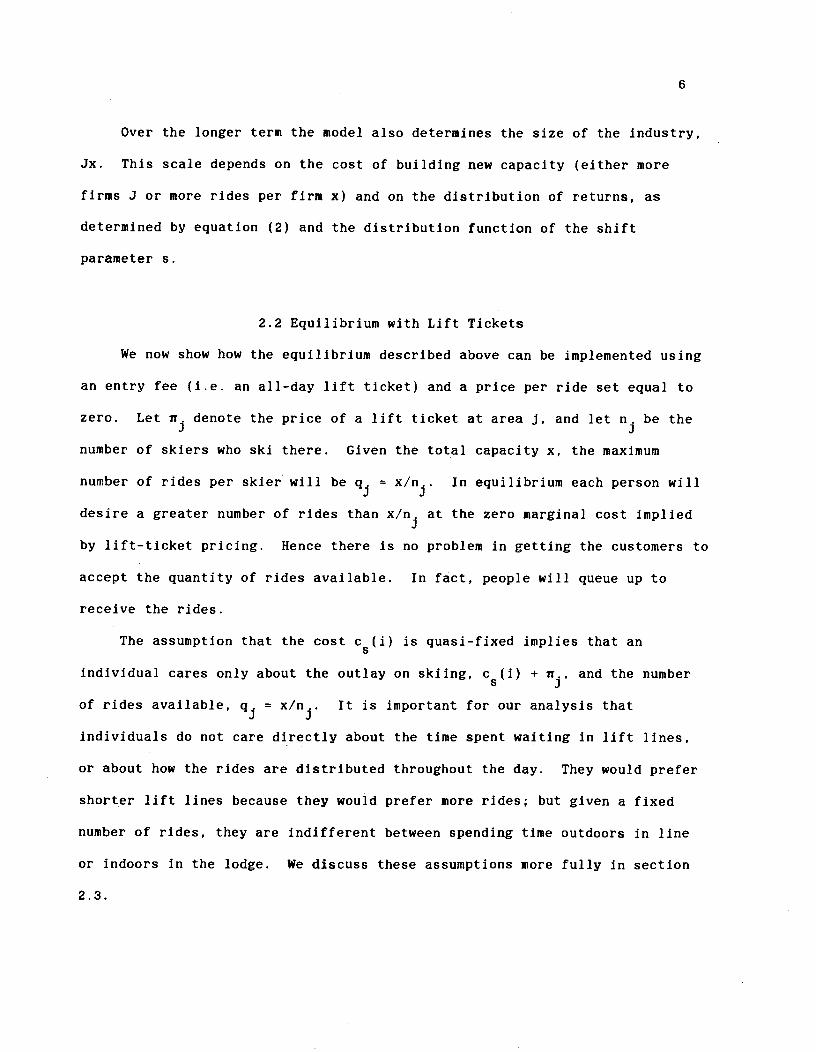
Over the longer term the model also determines the size of the industry,

Jx. This scale depends on the cost of building new capacity (either more

firms J or more rides per firm x) and on the distribution of returns, as

determined by equation (2) and the distribution function of the shift

parameter s.

2.2 Equilibrium with Lift Tickets

We now show how the equilibrium described above can be implemented using

an entry fee (i.e. an all-day lift ticket) and a price per ride set equal to

zero. Let n. denote the price of a lift ticket at area j, and let n. be the

number of skiers who ski there. Given the total capacity x, the maximum

number of rides per skier will be q. = x/n.. In equilibrium each person will

desire a greater number of rides than x/n. at the zero marginal cost implied

by lift-ticket pricing. Hence there is no problem in getting the customers to

accept the quantity of rides available. tn fact, people will queue up to

receive the rides.

The assumption that the cost c(i) is quasi-fixed implies that an

individual cares only about the outlay on skiing, c(i) + n.,, and the number

of rides available, q3 = x/n3. It is important for our analysis that

individuals do not care directly about the time spent waiting in lift lines,

or about how the rides are distributed throughout the day. They would prefer

shorter lift lines because they would prefer more rides; but given a fixed

number of rides, they are indifferent between spending time outdoors in line

or indoors in the lodge. We discuss these assumptions more fully in section

2.3.

7

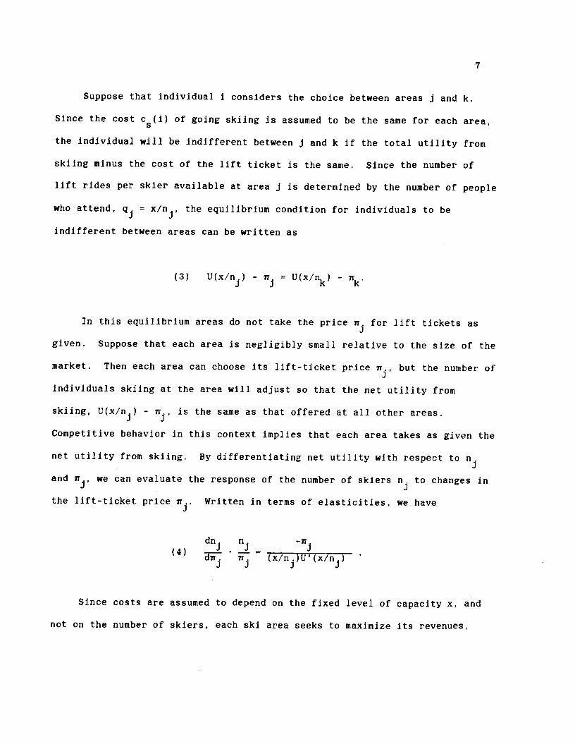
Suppose that individual I considers the choice between areas j and k.

Since the cost c(I) of going skiing is assumed to be the same for each area,

the individual will be Indifferent between j and k if the total utility from

skiing minus the cost of the lift ticket is the same. Since the number of

lift rides per skier available at area j is determined by the number of people

who attend, q3 = c/flj the equilibrium condition for individuals to be

indifferent between areas can be written as

(3) U(x/n.) - = U(x/nk) -

In this equilibrium areas do not take the price T. for lift tickets as

given. Suppose that each area is negligibly small relative to the size of the

market. Then each area can choose its lift-ticket price ir., but the number of

individuals skiing at the area will adjust so that the net utility from

skiing, U(x/n) - n., is the same as that offered at all other areas.

Competitive behavior in this context implies that each area takes as given the

net utility from skiing. By differentiating net utility with respect to

and flj we can evaluate the response of the number of skiers n to changes in

the lift-ticket price it3. Written in terms of elasticities, we have

dnn _________—

(x/n.)iY(x/n.)

Since costs are assumed to depend on the fixed level of capacity x, and

not on the number of skiers, each ski area seeks to maximize its revenues,

8

fl3flj taking as given the relation between the ticket price and the number of

skiers implied by equation (4). As usual, maximization of revenue requires

that the elasticity of customers flj with respect to the price be equal to

-1. so that in equilibrium we have

iT

(5) = U'(q ).

q3 j

The left side of equation (5) is the lift-ticket price,ii,

divided by

the number of rides per person at area j, q = x/n. For convenience, define

the effective price per ride under lift-ticket pricing as

(6) =

The right side of equation (5) is the marginal valuation of' rides, U',

evaluated at the quantity q.. Because the demand curve D(') is simply the

inverse of marginal utility, each person at area j ends up with the quantity

from the demand curve q. that corresponds to the effective price per ride

Although people wait in line and face an explicit marginal cost for rides of

zero, the results are as if each skier gets the quantity of rides that he or

she would demand at an explicit market price per ride . That is, equation

(5) can be rewritten as

(7) qj = D().

9

Each area sets prices according to equation (5) and each must provide a

given level of the net utility term, U(x/n.) - n.. Since the areas have the

same capacity x and are otherwise identical, they end up with the same values

for the lift-ticket price, u. = ur, the number of customers, n = N/J, and the

effective price per ride, . =

To complete the description of the equilibrium, it remains to determine

the value of the common lift-ticket price, iT, or equivalently of the effective

price per ride . We can analyze the decision to incur the fixed cost to go

skiing just as In the first model, except that the explicit price per ride P

Ais now replaced by the effective price P. (Recall from equation (7) that

people end up with the quantity of rides that they would demand at this

price.) The analogue to equation (1)—which determined the total number of

skiers N in the first model—is

(8) N = N() = c{U[D()J -

In equilibrium the effective price per ride is such as to equate the total

capacity for rides, Jx, to the total demand, qN, which implies

(9) Jx = D().N() = D()'c{U{D()J -

Since this is the same equation that determined the price per ride P in the

first equilibrium, the effective price takes on the same value. Finally,

equations (6) and (7) imply that the common lift-ticket price is determined by

the effective price per ride,

10

A A A(10) n = Pq = P.D(P).

Since the equilibrium with lift-ticket pricing yields an effective price

Aper ride P equal to the explicit price per ride P in the first equilibrium,

skiers receive the same number of rides at the same cost in each case. The

same people end up participating, and each ski area receives the same revenue.

The equality of and flj across areas is special to the example here.

Section 3 shows that and n can vary across areas If' there are differences

in skiers' preferences, U.(), or in the characteristics of ski areas. What

does generalize is the result that the lift-ticket equilibrium can replicate

the quantities and effective prices from a ride-ticket equilibrium where

prices are set equal to marginal valuations and no quantity constraints are

present.

In the longer run context where the capacity Jx Is variable, suppliers

have the same incentives to Invest under lift-ticket pricing as they did in

the first model. Specifically, the effective price per ride correctly

corresponds to the skiers' marginal valuation of rides, U'. Thus—given our

assumption that people care about the number of rides but not directly about

the time spent in line—there are no Inefficiencies implied by the existence

of queues, which reflect the explicit marginal cost of zero for rides.

Allocative decisions are still based on the proper shadow price, = U'(q).

Although the lift-ticket equilibrium is fundamentally only a repackaged

form of the original competitive equilibrium, the superficial appearances are

strikingly different. Specifically, the lift-ticket solution features

11

quantity rationing by means of queues, as well as ticket prices that seem to

be set by firms with market power. A regulator might note with Concern that

the "demand' for lift tickets at each area is the downward-sloping curve

determined by equation (4), and that each area maximizes revenue

subject to this curve.

2.3 Ride Tickets versus Lift Tickets

Given the assumptions so far, there Is no basis for predicting which of

the two forms of pricing will be observed. They lead to identical allocations

and effective prices. Ski areas charging on a per ride basis could coexist

with others charging on a lift-ticket basis. One can readily verify that an

area could also use a combination of a lift ticket (i.e. an entry fee) and a

charge per ride.

The description of the world implicit in this model misses important

features of reality. For some aspects, such as the determination of the price

per ride P or , these features may be unimportant. However, in the choice

between two otherwise equivalent pricing schemes, these featuresmay be

decisive. The most obvious elements neglected so far are:

a) the costs that must be incurred by an area to enforce Contracts,

for example, to avoid the theft of rides;

b) rides are not homogenous, but are heterogeneous goods Indexed by

the time of day and by Contingencies such as breakdowns and arrivals

of skiers;

c) time spent waiting in line Is likely to have a positive

opportunity cost.

12

We can conjecture what the Inclusion of these features would imply.

Given the allocation of rides common to the two kinds of equilibria (and to

any mixture of these two), the form of pricing that minimizes the neglected

costs will be selected. Ride-ticket pricing will generally have higher

monitoring and set-up costs than lift-ticket pricing. Since it would be

extremely expensive to set up a complete series of markets In time and.

contingency specific rides and to enforce contracts written in this form, some

amount of queuing would be expected even under pure ride pricing. On the

other hand, lift-ticket pricing imposes costs in terms of time. Relative to a

system with an extensive system of reservations for lift rides at specified

times, each individual must spend more time at a ski area to achieve the given

allocation of rides. However, if the typical skier's fixed cost, c, for

getting to the ski area Is large, then this last element would be relatively

unimportant.

As far as we know, ski areas use only the lift-ticket form of pricing. 01

(1971) describes how Disneyland once followed a combination form of pricing

with an entry fee and a per ride fee. (In contrast to the explanation offered

here, 01 Interprets this scheme as evidence of market power.) Disneyland has

since shifted to a pure entry fee. We take these observations as evidence

that the costs of allocating rides using ride tickets are higher than those

using entry fees. Presumably the cost of Implementing reservations and

collecting ride tickets outweigh the value of the savings in the time required

to acquire a given number of rides. This outcome is especially likely If' the

lump-sum costs of participating are large, and If time spent at a ski area or

amusement park is valued for its own sake.

13

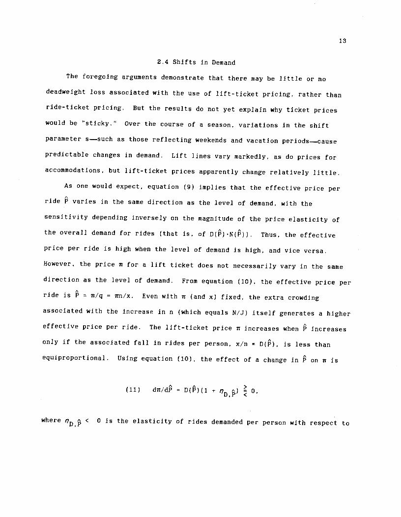
2.4 Shifts in Demand

The foregoing arguments demonstrate that there may be little or no

deadweight loss associated with the use of lift-ticket pricing, rather than

ride-ticket pricing. But the results do not yet explain why ticket prices

would be "sticky." Over the course of a season, variations in the shift

parameter s—such as those reflecting weekends and vacation periods—cause

predictable changes in demand. Lift lines vary markedly, as do prices for

accommodations, but lift-ticket prices apparently change relatively little.

As one would expect, equation (9) implies that the effective price perA

ride P varies in the same direction as the level of demand, with the

sensitivity depending inversely on the magnitude of the price elasticity of

A Athe overall demand for rides (that is, of D(P)•N(p)). Thus, the effective

price per ride is high when the level of demand is high, and vice versa.

However, the price n for a lift ticket does not necessarily vary in the same

direction as the level of demand. From equation (10), the effective price per

ride is = n/q = rn/x. Even with ii (and x) fixed, the extra crowding

associated with the increase in n (which equals N/J) itself generates a higher

Aeffective price per ride. The lift-ticket price ir increases when P increases

only if the associated fall in rides per person, x/n = D(), is less than

equiproportional. Using equation (10), the effect of a change in on is

(11) dn/d = D()(1 + 0,

where < 0 is the elasticity of rides demanded per person with respect to

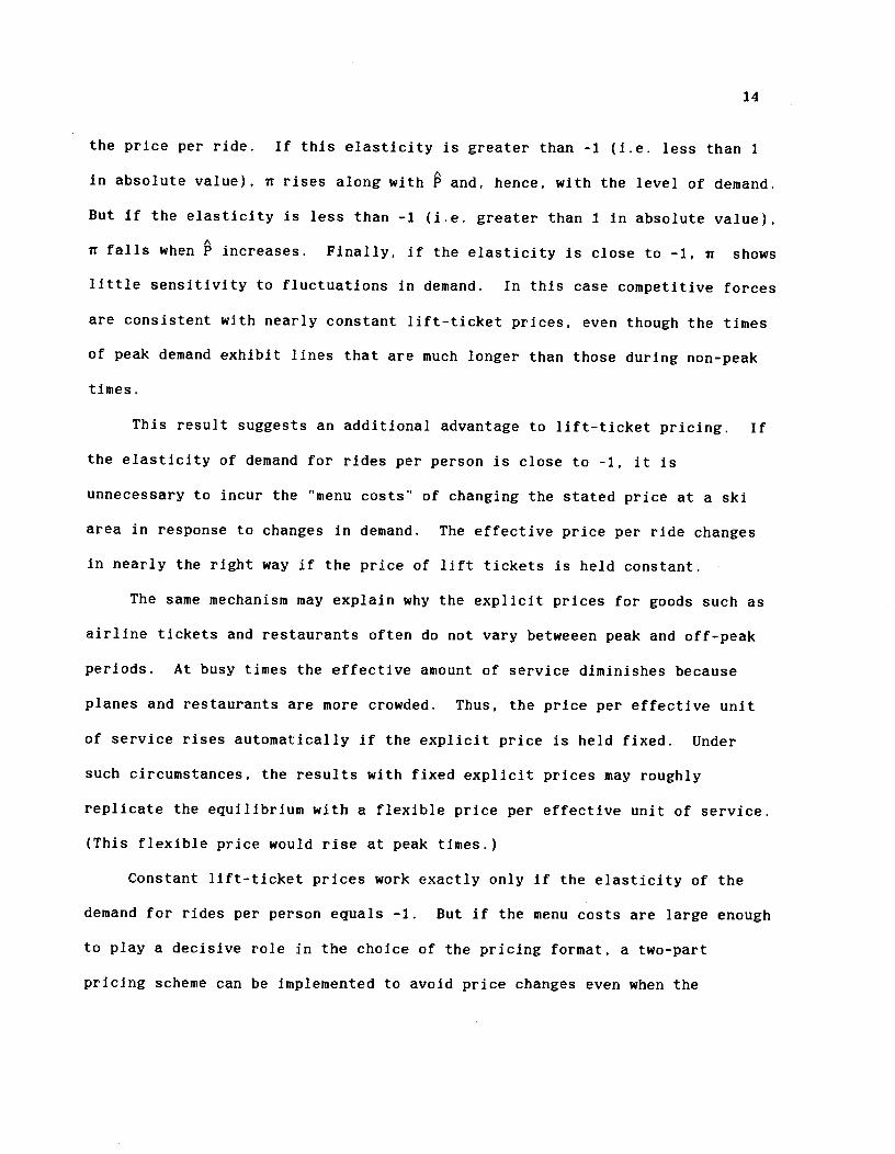
14

the price per ride. If this elasticity Is greater than -1 (i.e. less than I

in absolute value), r rises along with and, hence, with the level of demand.

But if the elasticity is less than -1 (i.e. greater than I In absolute value),

n falls when increases. Finally, if the elasticity is close to -1, n shows

little sensitivity to fluctuations in demand. In this case competitive forces

are consistent with nearly constant lift-ticket prices, even though the times

of peak demand exhibit lines that are much longer than those during non-peak

times.

This result suggests an additional advantage to lift-ticket pricing. If

the elasticity of demand for rides per person is close to -1, it is

unnecessary to incur the "menu costs' of changing the stated price at a ski

area in response to changes in demand. The effective price per ride changes

in nearly the right way if the price of lift tickets is held constant.

The same mechanism may explain why the explicit prices for goods such as

airline tickets and restaurants often do not vary betweeen peak and off-peak

periods. At busy times the effective amount of service diminishes because

planes and restaurants are more crowded. Thus, the price per effective unit

of service rises automatically If the explicit price is held fixed. Under

such circumstances, the results with fixed explicit prices may roughly

replicate the equilibrium with a flexible price per effective unit of service.

(This flexible price would rise at peak times.)

Constant lift-ticket prices work exactly only if the elasticity of the

demand for rides per person equals -1. But if the menu costs are large enough

to play a decisive role in the choice of the pricing format, a two-part

pricing scheme can be implemented to avoid price changes even when the

15

elasticity differs from -1. This consideration does not appear to be relevant

for ski areas, where per ride charges do not seem to be used, but may be a

factor in the choice of such a scheme by some amusement parks.

To see how this would work, consider an amusement park with capacity x,

which charges an entry fee ii and a price per ride r. Exactly as was the case

for a ski area, if the park is small relative to the industry as a whole, it

takes the net utility level for attending the park, U[D()J - 'D(), as

given. Hence, the park cannot change the effective price pez ride

However, it does not take as given the number of people attending or the price

of the admission ticket. When n people visit the park, the supply of rides

per person Is x/n and the effective price per ride is r + nn/x. Since the

effective price must equal and since the number of rides demanded must equal

the demand, D(),' the set of possible combinations of r and ir is given by the

relation,

A A(12) P = r ÷ ir/D(P).

For fixed r, this equation determines how ii must vary with the changes in

that are induced by changes in demand. The analogue to equation (10) above is

(13) n = (-r)D(),

1Note that, since >r, the demand at the explicit price r, D(r), exceeds the

quantity available, q=D(). Therefore, although the explicit price is nowpositive, the demanders still queue up for the available rides. These queuestypically applied at Disneyland, even when ride tickets were used.

16

and the analogue to equation (11) is

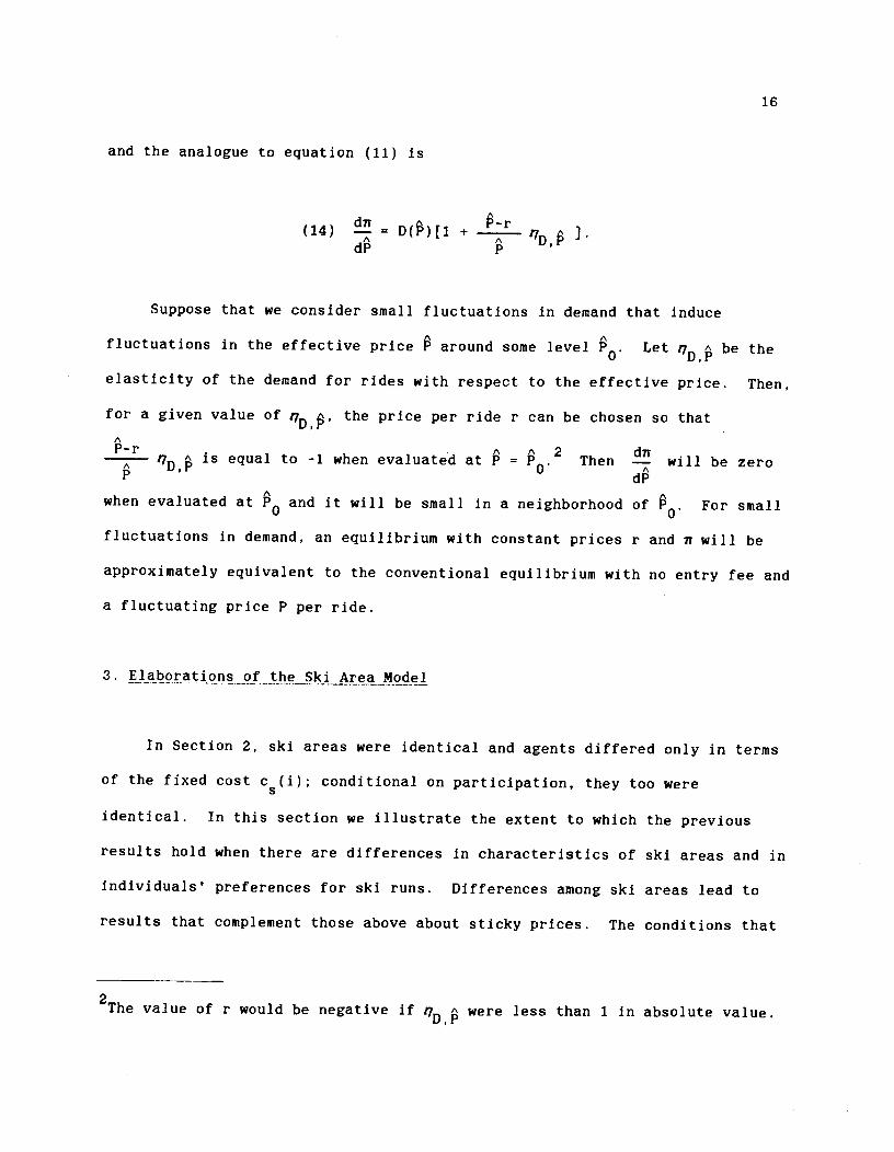
dir A(14) — = D(P)[1 +

AdP P

Suppose that we consider small fluctuations in demand that induce

fluctuations In the effective price around some level . Let be the

elasticity of the demand for rides with respect to the effective price. Then,

for a given value of the price per ride r can be chosen so that

AP-r A A 2 dirA D is equal to -1 when evaluated at P =

P0. Then — will be zeroP dP

when evaluated at and it will be small in a neighborhood of . For small

fluctuations in demand, an equilibrium with constant prices r and ir will be

approximately equivalent to the conventional equilibrium with no entry fee and

a fluctuating price P per ride.

3. Elaborations of the Ski Area Model

In Section 2, ski areas were identical and agents differed only in terms

of the fixed cost c(i); conditional on participation, they too were

identical. In this section we Illustrate the extent to which the previous

results hold when there are differences in characteristics of ski areas and in

individuals' preferences for ski runs. Differences among ski areas lead to

results that complement those above about sticky prices. The conditions that

2The value of r would be negative if were less than 1 in absolute value.

17

cause lift-ticket prices to be invariant with demand also cause these prices

to be the same at areas with different characteristics. However, differences

in preferences can lead to differences in ticket prices among areas, even if

the areas are identical.

3.1. Differences Among Ski Areas.

Consider a pool of N identical skiers who have decided to go skiing.

These skiers choose among J areas, indexed by j. Let b. denote the cost for

any skier to travel to area j; for example, b. could be determined by the

distance of the area from a major urban center. Ski areas may also differ in

terms of the length or 'quality' of their ski runs. We represent these

differences by assuming that area j has the capacity x, which is measured in

terms of numbers of runs of a specified length (or quality). When modeled in

this way, the differences across areas in x turn out to add little to the

analysis. For a given value of the transportation cost, b.., an increase in x.

leads solely to a one-for-one change in the number of skiers who come to area

j. That is, variations in x. do not lead to variations across areas in the.3

number of standardized ski runs per skier or in the price per standardized ski

run.

As before, is the lift-ticket price and q. = x/n. is the number of

rides (of standardized length) per person at area j. For an individual to be

Indifferent between areas j and k, it must be that

(15) U(q) - - b. U(q) - - bk.

18

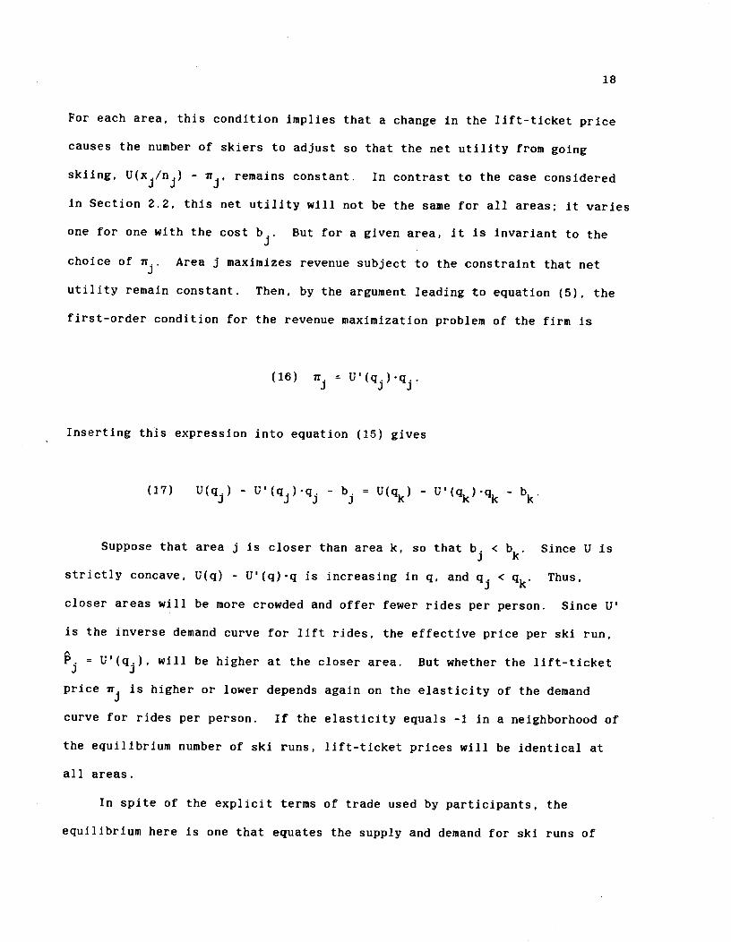
For each area, this condition implies that a change in the lift-ticket price

causes the number of skiers to adjust so that the net utility from going

skiing, U(x./n) - iT, remains constant. In contrast to the case considered

in Section 2.2, this net utility will not be the same for all areas; it varies

one for one with the cost b. But for a given area, it is invariant to the

choice of n3. Area j maximizes revenue subject to the constraint that net

utility remain constant. Then, by the argument leading to equation (5), the

first-order condition for the revenue maximization problem of the firm is

(16) =U'(q.).q.

Inserting this expression into equation (15) gives

(17) U(q.) - U'(q)•q.- b. = U(q) - U'().q -

bk.

Suppose that area j is closer than area k, so that b < bk. Since U is

strictly concave, U(q) - U'(q).q is increasing in q, and q. < Thus,

closer areas will be more crowded and offer fewer rides per person. Since U'

is the inverse demand curve for lift rides, the effective price per ski run,

= U'(q.), will be higher at the closer area. But whether the lift-ticket

price is higher or lower depends again on the elasticity of the demand

curve for rides per person. If the elasticity equals -1 in a neighborhood of

the equilibrium number of ski runs, lift-ticket prices will be identical at

all areas.

In spite of the explicit terms of trade used by participants, the

equilibrium here is one that equates the supply and demand for ski runs of

19

standardized length, not the supply and demand for all-day lift tickets. The

last result illustrates the importance of this distinction. If' one thinks in

terms of a demand for lift tickets, one is naturally led to the incorrect

conclusion that the ticket price should vary one for one with the cost b. so

that 1T÷b would be the same for all areas. If this total cost of going

skiing were the same at all areas, and the number of ski runs per person q.

were also the same, individuals would be indifferent between areas; that is,

equation (15) would be satisfied.

To see why this cannot be an equilibrium, it is useful to consider the

analysis from the viewpoint of a social planner. By the first welfare

theorem, a competitive equilibrium with ride tickets is Pareto optimal.

3There are two equivalent ways to see why this is so. The first is to notethat linearity of utility in other goods effectively converts the Paretoproblem into a problem with transferable utility. Therefore, the optimum mustmaximize total utility. Redistribution takes place by means of transfers ofincome. Alternatively, note that the function 13(q) measures the area underthe demand curve for lift rides. The sum of these functions Is the usualmeasure of aggregate consumer surplus, and quasi-linear utility was chosenprecisely because It permits a simple Marshallian analysis of our problem.

Because we assume that total utility is linear in income, we can calculate the

unique, Pareto optimal allocation of ski rides by maximizing an unweighted sum

over Individuals of the utility from skiing minus the cost of going skiing.3

With N identical skiers and J ski areas indexed on the interval [O,J}, the

planner must choose the number of skiers n at each area. The problem is then

to maximize the integral,

20

J0 [nU(x./n)-

n3bJ dj,

subject to the constraint

J

5 n.dj = N.

At the suggested allocation where q = x./n. is the same at all areas,

individuals get the same utility from skiing at each area. At the margin, the

planner could shift skiers from distant areas to closer ones with no loss in

satisfaction from skiing, but in so doing would reduce total transportation

costs. Thus this cannot be the social optimum. Using the substitution

= x/n., a quick calculation demonstrates that the first-order condition

for this problem is precisely equation (17). To support this optimum, it

makes no difference whether areas charge the price per standardized ski run of

P. = U'(q.), or offer q. runs at a price n. =

The next section shows that differences in individual preferences cause

lift-ticket prices to vary among areas. But to the extent that these

differences are small, the present observation permits a kind of

cross-sectional check on the explanation proposed above for the stickiness of

lift-ticket prices. Many explanations can be offered for price stickiness

over time, but it is harder to explain cross-sectional stickiness. If the

demand curve for ski runs per person is close to being unit elastic, then

there should be less variation in lift-ticket prices than in the number of

skiers or the length of lift lines, both in comparisons over time and among

21

areas at a point in time. In both dimensions, it will appear that quantities

respond more than prices.

3.2. Differences in Preferences

Suppose now that utility as a function of lift rides, U1(q), differs

among individuals. At an effective price per ride , the demand for rides per

person, D1(), also differs. All of the previous equilibria deliver the same

number of rides to all skiers at a given area by means of a queuing mechanism.

Since this mechanism does not discriminate among people with different

preferences, It cannot allocate different numbers of rides per day, D.(), to

them. To achieve an allocation that does discriminate, different areas (or

different classes of tickets at a single area) will have to cater to different

types of individuals.

Consider again the case where ski areas are identical. For simplicity we

deal with only two types of consumers: there are N1 agents with preferences

tJ1(q) = u(q), and N2 agents with preferences U2(q) = cu(q), where a > 1.

Thus, type 2 indIviduals are more avid skiers. Think again of a social

planner, who Is free to allocate skiers among areas. Assume that type one

skiers are allocated to areas in the interval [O,J1J, and type 2 skiers to the

interval [J1,J]. Simple arguments show that the number of skiers should be

the same for all areas In a given interval. Since the total capacity of areas

serving type 1 skiers is J1x, and that serving type 2 skiers is [J-J1]x, the

planning problem reduces to choosing J1 to maximize the sum

(18) N1U1(J1x/N1) + N2U2[(J-J1)x/N2]=

N1u(J1x/N1)+

N2cu[(J-J1)x/N2).

22

As one would expect from an analysis of the demand for rides, the first-order

condition for this problem implies that the marginal utility of a ride is the

same at each area, U(q1) = t(g2).As in the analysis of Section 2, competition among areas using

lift-ticket pricing will lead to lift-ticket prices =U(q1)•q1, and

=U(q2).q2. In general, these prices need not be the same. In the case

where u(q) = ln(q), so that the demand curve for each type of individual is

unit elastic, we have q2 oq1 and =an1. In this case, the areas catering

to type two skiers charge a higher lift-ticket price and offer more rides per

person. In general, the areas with high ticket prices are less crowded and

attract more avid skiers (that is, people who are willing to pay more per ski

run).

Each ski area still meets the effective price per ride,

=U(q1) = U(q2), just as if it charged this price directly. Moreover,

each area faces a given capacity constraint x. Since x/n, the number of

rides per person, times , the effective price per ride, must equal the ticket

price n, the number of customers who show up as a function of the ticket price

is

(19) n = XP/ir.

Therefore, over the range of values for that are observed in equilibrium,

each area faces a demand in terms of numbers of skiers, flj. that has an

elasticity of precisely -l with respect to the lift-ticket price ir..

Correspondingly, the areas revenue, nn = x, is invariant with respect to

23

the choice of the ticket price from the set of ticket prices that are

observed In equilbrluin. The areas are indifferent between charging a high

price and catering with short lines to the skiers who demand lots of' rides per

person, or charging a low price and servicing with long lines those who demand

ew rides.

This equiproportional change in the number of skiers in response to a

change In the lift-ticket price does not depend on the elasticity of the

aggregate demand curve for lift rides. It obtains whenever a range of

lift-ticket prices is observed in equilibrium. As an area changes its

lift-ticket price, It also changes the entire class of skiers that choose to

patronize it.

Except for the restriction to a finite number of individual types, and

hence a finite number of observed prices jr., the lift-ticket equilibrium in

the presence of different tastes resembles the equilibrium with differentiated

products and hedonic prices as described In Rosen (1974). Each type of ski

area offers a different type of skiing experience, Indexed by q., the number

of ski runs available per skier. With identical competitive producers, profit

is invariant to the type of good offered, and the price function Tr(q) traces

out the structure of the demand side of the market. In Rosen's model,

producers with no market power choose the type of good offered and the price

charged from the locus described by ir(q). Here, the departure from the

appearance of price-taking behavior Is even sharper. Firms simply choose a

price n; quality adjusts endogenously. It Is interesting to note that, until

recently, the Metro in Paris used a similar scheme to sort people by taste.

Purchasers of first-class tickets rode in separate cars, which were not

24

physically different from second-class cars, except that the first-class cars

were less crowded (in equilibrium).4 Roughly speaking, individuals with a

stronger preference for ski rides or with a greater distaste for congestion

are willing to pay more for the opportunity to pay more.

4. pp1IcatIon to the_Labor Market

In this section we apply the paradigm of ski-lift pricing to the labor

market. In this context a fully flexible wage rate corresponds to a flexible

price per lift ride. The case of a lift ticket relates to alternative methods

of labor compensation, such as profit-sharing schemes. From the standpoint of

an individual worker, the firm's total profit looks like a ski operator's

total capacity. In particular, the amount that each person gets (share of

profits or number of lift rides) varies inversely with the number of other

people who show up. (Profit per worker falls with more workers as long as the

average product of labor exceeds the marginal product.) But, as in the ski

example, competition among firms causes the parameters of the profit-sharing

rule to adjust so as to reproduce the outcomes that would emerge under

flexible wages. Further, at least as an approximation, It Is satisfactory to

have fixed wages and fixed parameters for the sharing formula. Thus—even in

the absence of any long-term contracts—these kinds of rigidities need not

imply any inefficiencies.

4We are told that the abolition of this vestige of the class system was one ofthe promises made In the presidential campaign of Francois Mitterand. Afterhis election, a compromise was reached whereby this system was not allowed tooperate during the morning and evening periods of peak demand (where itpresumably would be most useful), but remained in effect during the middle ofthe day.

25

Suppose that each of J identical, competitive firms has the production

function,

(20) Y = A.F(n),

where Y is output, A is a technological shift parameter, and n is the number

of workers. We assume that each worker works a fixed number of hours per day.

Given the real wage rate w, profit maximization for each firm entails

(21) F'(n) = w/A.

Equation (21) determines each firm's labor demand. Aggregate labor demand is

the multiple J of the demand per firm.

The economy has a population of M potential workers. Those who work

consume the quantity q = w+R, where R is non-wage (profit) income. Those who

do not work consume the amount q = R. Utility for person i Is given by

U[q(i)J - c(i), where c(i) is the reservation wage. As before, we think of

the index I as running over the continuum, [0,MJ, with c(i) increasing in 1.

Assuming that w and R are the same for all persons, individual i works if

IJ(w÷r) - U(R) exceeds c(i). Hence, aggregate labor supply can be written as

(22) N = c1[U(w+r) - U(R)}.

For a given distribution of reservations wages and a given value of R, the

slope of the labor-supply function Is (c1)' > 0.

The equation of aggregate labor suply to aggregate labor demand

determines the market-clearing values of the wage rate, w*, and employment, N*

(which we assume to be less than the potential population M). Then each

firm's employment is n* = N*/J. We assume that variations In wages rates and

employment reflect shifts in the technological parameter A, and we make

assumptions on preferences which guarantee that an increase in A causes an

26

increase In employment. Equations (21) and (22) imply that an increase in A

leads to an increase in w. If the production function F is strictly concave,

profits will also increase, which we assume raises the value of R for each

potential worker. In equation (22), an Increase in w, with R held constant,

causes N to increase by the usual substitution effect. An increase In R

causes N to fall by the positive income effect on the demand for leisure. We

assume that the substitution effect from a higher w is dominant, which Is

especially likely if the technological disturbance Is temporary. If we define

to be the elasticity of x with respect to y, it follows that

0 and 0 A<For concreteness we focus on technological shocks, but we could equally

well have assumed other types of exogenous shocks. We have also assumed

implicitly that the market for goods is competitive, but this assumption Is

also not crucial. We could have used instead the kind of monopolistically

competitive market structure assumed by Weitzman (1985). All that matters for

our analysis Is that workers and firms lack market power in the labor market,

and that employment and the marginal product of workers move together.

As In the ski-lift example, the competitive equilibrium in the labor

market can be supported by pricing mechanisms other than the obvious one of

freely flexible wage rates per worker. For example, assume that the wage rate

is fixed at some value w' < w. The wage w' parallels the explicit price per

ride, r, in the ski-lift case. Therefore, w' = 0 corresponds to pure

lift-ticket pricing, where r = 0.

5From equation (21), > 0 implies < 0, which implies '7wA < •

27

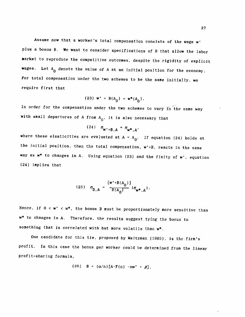
Assume now that a worker's total compensation consists of the wage w'

plus a bonus B. We want to consider specifications of B that allow the labor

market to reproduce the competitive outcomes, despite the rigidity of explicit

wages. Let A0 denote the value of A at an initial position for the economy.

For total compensation under the two schemes to be the same initially, we

require first that

(23) w' +B(A0)

=w*(A0).

In order for the compensation under the two schemes to vary in the same way

with small departures of A from A0, it is also necessary that

(24) '7w'÷B,A =

where these elasticities are evaluated at A =A0. If equation (24) holds at

the initial position, then the total compensation, w'4-B, reacts in the same

way as w to changes in A. Using equation (23) and the fixity of w', equation

(24) implies that

[w'÷B(A0)](25) '7B,A =

B(A0) '7w*,A

Hence, if 0 < w' < w, the bonus B must be proportionately more sensitive than

w to changes in A. Therefore, the results suggest tying the bonus to

something that is correlated with but more volatile than w.

One candidate for this tie, proposed by Weitzman (1985), is the firm's

profit. In this case the bonus per worker could be determined from the linear

profit-sharing formula,

(26) B = (/n)[A•F(n) -nw' --

28

where a and e are parameters. If a and/or O were flexible, then—as in the

ski-lift example—competition would ensure the adjustments necessary to

support the employment level n* at each firm. If a and are restricted to be

constants (that is, invariant with respect to A), then the necessary values of

these parameters follow from equations (23) and (25). In particular, for a

given value of w', we can show that 0 < a < I and 6 Further, given the

other parameters of the problem, it is possible to choose a value of w' < wsuch that 13 = 0, in which case the profit-sharing rule takes the simple form

described by Weitzman.7 In any event, If a and 13 are such that equations (23)

and (25) are satisfied, then—at least locally—the fluctuations in total

compensation correspond to the fluctuations in w, and thereby support the

variations In n* that would have resulted with flexible wages.

In this solution workers face the explicit wage w' < w (w' = 0 is

possible), but also get a share of the profits. In deciding whether to work,

each person looks only at his own total compensation and neglects the fact

6The result for a is

[w*z7 A+ (w*_w)i7 A1a

[A.F(n)/n ÷ (W*_WI)n*Al

where a < 1 follows because A•F(n)/n > w and < 1. The result for 13 Is

(w*_w')AF(n)/n - (w*_w')[AF(n)/n - wIlls A- w5[AF(n)/n -

W')17W*A >

Wtlw*A+

(w*_w')llfl*,A

(13 < 0 applies If w5 = w'.) All expressions above are evaluated at someinitial position, denoted before by the superscript 0.

7However, the necessary value of w' could be negative. See the formula for13/n in n.6 above.

29

that his participation reduces the profit distributed to the other workers

(which occurs if the marginal product of labor is below the average product).

This interaction parallels the negative effect of an additional skier's

participation on the rides available for others. Nevertheless, as in our

previous example for skiing, the appropriate profit-sharing scheme reproduces

the results for employment and total compensation per worker that would arise

under flexible wages. (This result is exact if a and/or ,G are flexible and

determined by the competitive interaction of firms. If a and are fixed, but

at the appropriate values, then the result holds locally.)

It also follows that firms would eagerly hire more workers than are

available at the going wage w' (< w*) and the prescribed terms for sharing

profits. (This result parallels the eagerness of skiers to queue up for lift

rides.) But more workers than n do not present themselves because the total

compensation, w'+B, would then fall below the value w, which is the

reservation wage of the marginal worker (when total employment is N* = Jn*).

As with flexible wages, employment is determined so that labor's marginal

product equals the competitive wage w. In other words, profits are maximized

subject to the constraint that firms pay each worker a total compensation that

equals the marginal worker's reservation wage. Thus, the outcomes are Pareto

optimal despite sticky wages and the apparent common-property problem

associated with the sharing of profits. Even though the marginal cost to the

firm of an additional worker is less under the profit-sharing arrangement, the

equilibrium level of employment is the same as that with flexible wages.

Correspondingly, the firms in each regime face the appropriate shadow price of

labor (w*), and thereby make correct decisions with respect to investment in

capital, entry and exit, etc.

30

A profit-sharing scheme will not work if disturbances sometimes cause

employment and wages to move in opposite directions. For example, this

pattern would emerge from shifts to workers' reservation wages. Even barring

such disturbances, the results do not imply that profit sharing is superior to

other schemes that allow the bonus (and thereby total labor compensation) to

move along with w. Also, the analysis does not suggest that a framework with

fixed wages and a flexible bonus (related, say, to profits) would be superior

to a setup with flexible wages. As was the case for ski areas, the choice of

compensation scheme must be based on elements of reality that are excluded

from this model.

One element that is not a candidate for explaining a preference for

profit sharing is a pure menu cost of changing the amount of compensation

received by each worker. Total compensation per worker is the same at every

point in time under any equivalent scheme, and there Is no reason to believe

that it is easier to vary bonuses than to vary wages. A more promising

approach may be to consider asymmetric information. If profits are observable

by workers, but a technological shock like A is not, then problems of

enforcement may lead to the selection of a contract that is contingent on

profits rather than on A. But this line of argument suggests that an

observable like total sales, which is less susceptible to manipulation by

firms, might be an even better choice. In any case, a call for the widespread

use of profit-sharing contracts and for subsidies to encourage their adoption,

as in Weitzman (1985), requires further analysis of why this System is more

attractive than alternatives, and why firms and workers do not settle

voluntarily on the preferred format for pricing.

REFERENCES

01, W. Y., /t Disneyland Dilemma: Two-Part Tariffs for a Mickey MouseMonopoly,' Quarterlyjourna1ofEcom1cs, 85, February 1971, 77-96.

Rosen, S., "Hedonic Prices and Implicit Markets," Journal_of PoliticalEconoml, 82, January/February 1974, 34-55.

Weitzman, M.L., "The Simple Macroeconomics of Profit Sharing," AmericanEconomic Review, 75, December 1985, 937-53.