NBER WORKING PAPER SERIES

MULTI-PERIOD CORPORATE DEFAULT PREDICTIONWITH STOCHASTIC COVARIATES

Darrell DuffieKe Wang

Leandro Saita

Working Paper 11962http://www.nber.org/papers/w11962

NATIONAL BUREAU OF ECONOMIC RESEARCH1050 Massachusetts Avenue

Cambridge, MA 02138January 2006

We are grateful for financial support from Moodys Corporation, The Federal Deposit Insurance Corporation,and The Department of Education of Japan. We have benefited from remarks from Takeshi Amemiya, SusanAthey, Richard Cantor, Brad Effron, Jeremy Fox, Peyron Law, Aprajit Mahajan, Ilya Strebulaev, the referee,and the editor. We are also grateful for data from Moodys Corporation and from Ed Altman. This paperextends earlier work by two of the authors under the title “Multi-Period Corporate Failure Prediction WithStochastic Covariates.” Duffie and Saita are at The Graduate School of Business, Stanford University. Wangis at The Faculty of Economics, The University of Tokyo. The views expressed herein are those of theauthor(s) and do not necessarily reflect the views of the National Bureau of Economic Research.

©2006 by Darrell Duffie, Ke Wang, and Leandro Saita. All rights reserved. Short sections of text, not toexceed two paragraphs, may be quoted without explicit permission provided that full credit, including ©notice, is given to the source.

Multi-Period Corporate Defualt Prediction With Stochastic CovariatesDarrell Duffie, Ke Wang, and Leandro SaitaNBER Working Paper No. 11962January 2006JEL No. C41, G33, E44

ABSTRACT

We provide maximum likelihood estimators of term structures of conditional probabilities of

corporate default, incorporating the dynamics of firm-specific and macroeconomic covariates. For

U.S. Industrial firms, based on over 390,000 firm-months of data spanning 1979 to 2004, the level

and shape of the estimated term structure of conditional future default probabilities depends on a

firm's distance to default (a volatility-adjusted measure of leverage), on the firm's trailing stock

return, on trailing S&P 500 returns, and on U.S. interest rates, among other covariates. Distance to

default is the most influential covariate. Default intensities are estimated to be lower with higher

short-term interest rates. The out-of-sample predictive performance of the model is an improvement

over that of other available models.

Darrell DuffieGraduate School of BusinessStanford UniversityStanford, CA 94305and NBERduffie@stanford.edu

Leandro SaitaGraduate School of BusinessStanford UniversityStanford, CA 94305lsaita@stanford.edu

Ke WangDepartment of EconomicsUniversity of Tokyo7-3-1 Hongo, Bunkyo-kuTokyo 113-0033 Japankewang@e.u-tokyo.ac.jp

1 Introduction

We provide maximum likelihood estimators of term structures of conditionalcorporate default probabilities. Our main contribution over prior work isto exploit the time-series dynamics of the explanatory covariates in orderto estimate the likelihood of default over several future periods (quarters oryears). We estimate our model for U.S.-listed Industrial firms, using over390,000 firm-months of data on over 2700 firms for the period 1979 to 2004.We find evidence of significant dependence of the level and shape of the termstructure of conditional future default probabilities on a firm’s distance todefault (a volatility-adjusted measure of leverage) and on U.S. interest ratesand stock-market returns, among other covariates. Variation in a firm’s dis-tance to default has a substantially greater effect on the term structure offuture default hazard rates than does a comparatively significant change inany of the other covariates. The shape of the term structure of conditionaldefault probabilities reflects the time-series behavior of the covariates, espe-cially leverage targeting by firms and mean reversion in macroeconomic per-formance. Out-of-sample predictive performance improves on that of otheravailable models, as detailed in Section 4.

Our model is based on a Markov state vector Xt of firm-specific andmacroeconomic covariates that causes variation over time in a firm’s defaultintensity λt = Λ(Xt), which is the conditional mean arrival rate of defaultmeasured in events per year. The firm exits for other reasons, such as mergeror acquisition, with an intensity αt = A(Xt). The total exit intensity is thusαt + λt. We specify a doubly-stochastic formulation of the point process fordefault and other forms of exit under which the conditional probability ofdefault within s years is

q(Xt, s) = E

(∫ t+s

t

e−R

z

t(λ(u)+α(u)) duλ(z) dz

∣

∣

∣

∣

Xt

)

. (1)

This calculation reflects the fact that a firm cannot default at time t if it hasalready disappeared for some other reason.

While there is a significant prior literature treating the estimation of one-period-ahead default (or bankruptcy) probabilities, for example with logitmodels, we believe that this is the first empirical study of conditional defaultprobabilities over multiple future time periods that incorporates the timedynamics of the covariates. The sole exception seems to be the practice of

1

treating the credit rating of a firm as though it is a Markov chain, with rat-ings transition probabilities estimated as long-term average ratings transitionfrequencies. It is by now well understood, however, that the current ratingof a firm does not incorporate much of the influence of the business cycleon default rates (Nickell, Perraudin, and Varotto (2000), Kavvathas (2001),Wilson (1997a), Wilson (1997b)), nor the important effect of prior ratingshistory (Behar and Nagpal (1999), Lando and Skødeberg (2002)). There is,moreover, significant heterogeneity in the short-term default probabilities ofdifferent firms of the same current rating (Kealhofer (2003)). As explainedin Section 4, the out-of-sample performance of ratings-based default proba-bilities are poorer than those of other available models. Of course, ratingscould be used in conjunction with other covariates, as in Carty (2000).

We anticipate several types of applications for our work, including (i) theanalysis by a bank of the credit quality of a borrower over various futurepotential borrowing periods, (ii) the determination by banks and bank regu-lators of the appropriate level of capital to be held by a bank, in light of thecredit risk represented by its loan portfolio, especially given the upcomingBasel II accord, under which borrower default probabilities play an explicitrole in capital requirements, (iii) the determination of credit ratings by rat-ing agencies, and (iv) the ability to shed some light on the macroeconomiclinks between business-cycle variables and the default risks of corporations.

Absent a model that incorporates the dynamics of the underlying covari-ates, one cannot extrapolate prior models of one-quarter-ahead or one-year-ahead default probabilities to longer time horizons. Campbell, Hilscher, andSzilagyi (2005) instead estimate separate logit models for default probabil-ities at each of a range of time horizons, although not taking advantage ofjoint consistency conditions across those horizons.1

The conditional default probability q(Xt, s) of (1) depends on:

• a parameter vector β determining the dependence of the default andother-exit intensities, Λ(Xt) and A(Xt), respectively, on the covariatevector Xt, and

• a parameter vector γ determining the time-series behavior of the un-derlying state vector Xt of covariates.

1Philosophov and Philiosophov (2002) estimate a model of default probabilities at var-ious horizons, although not exploiting the time dynamics of the covariates.

2

The doubly-stochastic assumption, stated more precisely in Section 2, isthat, conditional on the path of the underlying state process X determiningdefault and other exit intensities, exit times are the first event times of inde-pendent Poisson processes.2 In particular, this means that, given the path ofthe state-vector process, the merger and default times of different firms areconditionally independent.

A major advantage of the doubly-stochastic formulation is that it allowsdecoupled maximum-likelihood estimations of β and γ, which can then becombined to obtain the maximum-likelihood estimator of the default prob-ability q(Xt, s), and other properties of the model, such as probabilities ofjoint default of more than one firm. Because of this decoupling, the resultingestimator of the intensity parameter vector β is the same as that of a con-ventional competing-risks duration model with time-varying covariates. Themaximum likelihood estimator of the time-series parameter vector γ woulddepend of course on the particular specification adopted for the behavior ofthe state process X. For examples, we could allow the state process X tohave GARCH volatility behavior, to depend on Markov chain “regimes,” orto have jump-diffusive behavior. For our specific empirical application, wehave adopted a simple Gaussian vector auto-regressive specification.

The doubly-stochastic assumption is overly restrictive to the extent thatdefault or another form of exit by one firm could have an important directinfluence on the default or other-exit intensity of another firm. This influencewould be anticipated to some degree if one firm plays a relatively large rolein the marketplace of another. The doubly-stochastic property does not fitthe data well, according to tests developed by Das, Duffie, Kapadia, andSaita (2005). Our empirical results should therefore be treated with caution.In any case, we show substantially improved out-of-sample performance overprior models. For example, the average accuracy ratio (as defined in Section4) for one-year-ahead out-of-sample default prediction by our model, over1993-2003, is 88%. Hamilton and Cantor (2004) report that, for 1999-2003,accuracy ratios based on Moody’s3 credit ratings average 65%, while allowingratings adjustments for placements on Watchlist and Outlook are 69%, andthose based on sorting firms by bond yield spreads average 74%. More details

2One must take care in interpreting this characterization when treating the “internalcovariates,” those that are firm-specific and therefore no longer available after exit, asexplained in Section 2.

3Kramer and Guttler (2003) report no statistically significant difference between theaccuracy ratio of Moodys and Standard-and-Poors ratings in a sample of 1927 borrowers.

3

on out-of-sample performance are provided in Section 4.Our methods also allow estimation of the likelihood, by some future date,

of either default or a given increase in conditional default probability. Thisand related transition-risk calculations could play a role in credit rating, riskmanagement, and regulatory applications. The estimated model can be fur-ther used to calculate probabilities of joint default of groups of firms, or otherproperties related to default correlation. In a doubly-stochastic setting, de-fault correlation between firms arises from correlation in their default inten-sities due to (i) common dependence of these intensities on macro-variablesand (ii) correlation across firms of firm-specific covariates. Our model under-estimates default correlation relative to average pairwise sample correlationsof default reported in DeServigny and Renault (2002).

Our econometric methodology may be useful in other subject areas re-quiring estimators of multi-period survival probabilities under exit intensitiesthat depend on covariates with pronounced time-series dynamics. Examplescould include the timing of real options such as technology switch, mortgageprepayment, securities issuance, and labor mobility. We are unaware of previ-ously available econometric methodologies for multi-period event predictionthat exploit the estimated time-series behavior of the underlying stochasticcovariates.

1.1 Related Literature

A standard structural model of default timing assumes that a corporationdefaults when its assets drop to a sufficiently low level relative to its liabilities.For example, the models of Black and Scholes (1973), Merton (1974), Fisher,Heinkel, and Zechner (1989), and Leland (1994) take the asset process to bea geometric Brownian motion. In these models, a firm’s conditional defaultprobability is completely determined by its distance to default, which is thenumber of standard deviations of annual asset growth by which the asset level(or expected asset level at a given time horizon) exceeds the firm’s liabilities.This default covariate, using market equity data and accounting data forliabilities, has been adopted in industry practice by Moody’s KMV, a leadingprovider of estimates of default probabilities for essentially all publicly tradedfirms. (See Crosbie and Bohn (2002) and Kealhofer (2003).)

Based on this theoretical foundation, it seems natural to include distanceto default as a covariate. Even in the context of a standard structural de-fault model of this type, however, Duffie and Lando (2001) show that if the

4

distance to default cannot be accurately measured, then a filtering problemarises, and the default intensity depends on the measured distance to de-fault and also on other covariates that may reveal additional informationabout the firm’s conditional default probability. More generally, a firm’sfinancial health may have multiple influences over time. For example, firm-specific, sector-wide, and macroeconomic state variables may all influencethe evolution of corporate earnings and leverage. Given the usual benefits ofparsimony, and especially given the need to model the joint time-series be-havior of all covariates chosen, the model of default probabilities estimatedin this paper adopts a relatively small set of firm-specific and macroeconomiccovariates.

Prior empirical models of corporate default probabilities, reviewed byJones (1987) and Hillegeist et al. (2004), have relied on many types of co-variates, both fixed and time-varying. Empirical corporate default analysisoriginated with Beaver (1966), Beaver (1968a), Beaver (1968b), and Altman(1968), who applied multivariate discriminant analysis. Among the covari-ates in Altman’s “Z-score” is a measure of leverage, defined as the marketvalue of equity divided by the book value of total debt. Distance to defaultis essentially a volatility-corrected measure of leverage.

A second generation of empirical work is based on qualitative-responsemodels, such as logit and probit. Among these, Ohlson (1980) used an “O-score” method in his year-ahead default prediction model.

The latest generation of modeling is dominated by duration analysis.Early in this literature is the work of Lane, Looney, and Wansley (1986) onbank default prediction, using time-independent covariates.4 These modelstypically apply a Cox proportional-hazard model. Lee and Urrutia (1996)used a duration model based on a Weibull distribution of default time. Theycompare duration and logit models in forecasting insurer insolvency, findingthat, for their data, a duration model identifies more significant variablesthan does a logit model. Duration models based on time-varying covari-ates include those of McDonald and Van de Gucht (1999), in a model ofthe timing of high-yield bond defaults and call exercises.5 Related durationanalysis by Shumway (2001), Kavvathas (2001), Chava and Jarrow (2004),and Hillegeist, Keating, Cram, and Lundstedt (2004) predict bankruptcy.6

4Whalen (1991) and Wheelock and Wilson (2000) also used Cox proportional-hazardmodels for bank default analysis.

5Meyer (1990) used a similar approach in a study of unemployment duration.6Kavvathas (2001) also analyzes the transition of credit ratings.

5

Shumway (2001) uses a discrete duration model with time-dependent co-variates. Computationally, this is equivalent to a multi-period logit modelwith an adjusted-standard-error structure. In predicting one-year default,Hillegeist, Keating, Cram, and Lundstedt (2004) also exploit a discrete du-ration model. By taking as a covariate the theoretical probability of defaultimplied by the Black-Scholes-Merton’s model, based on distance to default,Hillegeist, Keating, Cram, and Lundstedt (2004) find, at least in this modelsetting, that distance to default does not entirely explain variation in defaultprobabilities across firms. This is supported by Bharath and Shumway (2004)and Campbell, Hilscher, and Szilagyi (2005), who find that in the presence ofmarket leverage and volatility information, among other covariates, distanceto default adds relatively little informatiom. Further discussion of the selec-tion of covariates for corporate default prediction may be found in Section3.2.

Moving from the empirical literature on corporate default prediction tostatistical methods available for this task, typical econometric treatments ofstochastic intensity models include those of Lancaster (1990) and Kalbfleischand Prentice (2002).7 In their language, our macro-covariates are “external,”and our firm-specific covariates are “internal,” that is, cease to be generatedonce a firm has failed. These sources do not treat large-sample properties, norindeed do large-sample properties appear to have been developed in a formsuitable for our application. For example, Berman and Frydman (1999) doprovide asymptotic properties for maximum-likelihood estimators of stochas-tic intensity models, including a version of Cramer’s Theorem, but treat onlycases in which the covariate vector Xt is fully external (with known transi-tion distribution), and in which event arrivals continue to occur, repeatedly,at the specified parameter-dependent arrival intensity. This clearly does nottreat our setting, for a firm typically disappears once it fails.8

7For other textbook treatments, see Andersen, Borgan, Gill, and Keiding (1992), Miller(1981), Cox and Isham (1980), Cox and Oakes (1984), Daley and Vere-Jones (1988), andTherneau and Grambsch (2000).

8For the same reason, the autoregressive conditional duration framework of Engle andRussell (1998) is not suitable for our setting, for the updating of the conditional probabilityof an arrival in the next time period depends on whether an arrival occured during theprevious period, which again does not treat a firm that disappears once it defaults.

6

2 Econometric Model

This section outlines our probabilistic model for corporate survival, and theestimators that we propose. The following section applies the estimator todata on U.S.-listed Industrial firms, and Section 4 discusses out-of-sampleperformance.

2.1 Conditional Survival and Default Probabilities

Fixing a probability space (Ω,F , P ) and an information filtration Gt : t ≥ 0satisfying the usual conditions,9 let X = Xt : t ≥ 0 be a time-homogeneousMarkov process in R

d, for some integer d ≥ 1. The state vector Xt isa covariate for a given firm’s exit intensities, in the following sense. Let(M,N) be a doubly-stochastic non-explosive two-dimensional counting pro-cess driven by X, with intensities α = αt = A(Xt) : t ∈ [0,∞) for M andλ = λt = Λ(Xt) : t ≥ 0 for N , for some non-negative real-valued measur-able functions A( · ) and Λ( · ) on R

d. Among other implications, this meansthat, conditional on the path of X, the counting processes M and N areindependent Poisson processes with conditionally deterministic time-varyingintensities, α and λ, respectively. For details on these definitions, one mayrefer to Karr (1991) and Appendix I of Duffie (2001).

We suppose that a given firm exits (and ceases to be observable) at τ =inft : Mt + Nt > 0, which is the earlier of the first event time of N ,corresponding to default, and the first event time of M , corresponding toexit for some other reason. In our application to U.S.-listed Industrial firms,the portion of exits for reasons other than default is far too substantial to beignored.

The main idea is that, so long as the firm has not exited for some reason,its default intensity is Λ(Xt) and its intensity of exit for other reasons isA(Xt).

It is important to allow the state vector Xt to include firm-specific de-fault covariates that cease to be observable when the firm exits at τ . Forsimplicity, we suppose that Xt = (Ut, Yt), where Ut is firm-specific and Yt

is macroeconomic. Thus, we consider conditioning by an observer whose in-formation is given by the smaller filtration Ft : t ≥ 0, where Ft is the

9See Protter (1990) for technical definitions.

7

σ-algebra generated by

(Us,Ms, Ns) : s ≤ min(t, τ) ∪ Ys : s ≤ t.

The firm’s default time is the stopping time T = inft : Nt > 0,Mt = 0.We now verify the formula (1) for default probabilities.

Proposition 1. On the event τ > t of survival to t, the Ft-conditionalprobability of survival to time t+ s is

P (τ > t+ s | Ft) = p(Xt, s) ≡ E

(

e−R

t+s

t(λ(u)+α(u)) du

∣

∣

∣

∣

Xt

)

, (2)

and the Ft-conditional probability of default by t+ s is

P (T < t+ s | Ft) = q(Xt, s),

where q(Xt, s) is given by (1).

Proof: We begin by conditioning instead on the larger information set Gt,and later show that this does not affect the calculation.

We first calculate that, on the event τ > t,

P (τ > t+ s | Gt) = E

(

e−R

t+s

t(λ(u)+α(u)) du

∣

∣

∣

∣

Xt

)

, (3)

and

P (T < t+ s | Gt) = q(Xt, s). (4)

The first calculation (3) is standard, using the fact that M +N is a doubly-stochastic counting process with intensity α+ λ. For the second calculation(4), we use the fact that, conditional on the path of X, the (improper)density, evaluated at any time z > t, of the default time T , exploiting theX-conditional independence of M and N is, with the standard abuse ofnotation,

P (T ∈ dz |X) = P (infu : Nu 6= Nt ∈ dz,Mz = Mt |X)

= P (infu : Nu 6= Nt ∈ dz |X)P (Mz = Mt |X)

= e−R

z

tλ(u) duλ(z) dz e−

R

z

tα(u) du

= e−R

z

t(α(u)+λ(u)) duλ(z) dz.

8

From the doubly-stochastic property, conditioning also on Gt has no effecton this calculation, so

P (T ∈ [t, t+ s] | Gt, X) =

∫ t+s

t

e−R

z

t(α(u)+λ(u)) duλ(z) dz.

Now, taking the expectation of this conditional probability given Gt only,using the law of iterated expectations, leaves (4).

On the event τ > t, the conditioning information in Ft and Gt coincide.That is, every event contained by τ > t that is in Gt is also in Ft. Theresult follows.

One can calculate p(Xt, s) and q(Xt, s) explicitly in certain settings, forexample if the state vector X is affine and the exit intensities have affine de-pendence on X. In our eventual application, however, the intensities dependnon-linearly on an affine process Xt, which calls for numerical computationof p(Xt, s) and q(Xt, s). Fortunately, this numerical calculation is done afterobtaining maximum-likelihood estimates of the parameters of the model.

2.2 Maximum Likelihood Estimator

We turn to the problem of inference from data.For each of n firms, we let Ti = inft : Nit > 0,Mit = 0 denote the default

time of firm i, and let Si = inft : Mit > 0, Nit = 0 denote the censoringtime for firm i due to other forms of exit. We let Uit be the firm-specific vectorof variables that are observable for firm i until its exit time τi = min(Si, Ti),and let Yt denote the vector of environmental variables (such as business-cycle variables) that are observable at all times. We let Xit = (Uit, Yt), andassume, for each i, that Xi = Xit : t ≥ 0 is a Markov process. (This meansthat, given Yt, the transition probabilities of Uit do not depend on Ujt forj 6= i, a simplifying assumption.) In our empirical implementation of themodel, we observe the covariates Xit only monthly or less frequently. Thismeans that Xit is constant between periodic observations, a form of time-inhomogeneity that involves a slight extension of our basic theory of Section2.1. We continue to measure time continuously, however, in order to takeadvantage of information on intra-period timing of exits.

Extending our notation from Section 2.1, for all i, we let Λ(Xit, β) andA(Xit, β) denote the default and other-exit intensities of firm i, where β is aparameter vector, common to all firms, to be estimated. This homogeneityacross firms allows us to exploit both time-series and cross-sectional data,

9

and is traditional in duration models of default such as Shumway (2001).This leads to inaccurate estimators to the degree that the underlying firmsare actually heterogeneous in this regard. We do, however, allow for hetero-geneity across firms with respect to the probability transition distributionsof the Markov covariate processes X1, . . . , Xn of the n firms. For example,some firms may have different target leverage ratios than others.

We assume that the exit-counting process (M1, N1, . . . ,Mn, Nn) of then firms is doubly-stochastic driven by X = (X1, . . . , Xn), in the sense ofSection 2.1, so that the exit times τ1, . . . , τn of the n firms areX-conditionallyindependent, as discussed in Section 1. There is some important loss ofgenerality here, for this implies that the exit of one firm has no direct impacton the default intensity of another firm. Their default times are correlatedonly insofar as their exit intensities are correlated.

The econometrician’s information set Ft at time t is

It = Ys : s ≤ t ∪ J1t ∪ J2t · · · ∪ Jnt,

whereJit = (1Si<u, 1Ti<u, Uiu) : t0i ≤ u ≤ min(Si, Ti, t)

is the information set for firm i, and where t0i is the time of first appearanceof firm i in the data set. For simplicity, we take t0i to be at the end of adiscrete time period and deterministic, but our results would extend to treatleft-censoring of each firm at a stopping time, under suitable conditionalindependence assumptions.

In order to simplify the estimation of the time-series model of covariates,we suppose that the environmental discrete-time covariate process Y1, Y2, . . .is itself a time-homogeneous (discrete-time) Markov process.

Conditional on the current combined covariate vectorXk = (X1k, . . . , Xnk),at period k, we suppose that Xk+1 has a joint density f( · |Xk; γ), for someparameter vector γ to be estimated. Despite our prior Markov assumption onthe covariate process Xik : k ≥ 1 for each firm i, this allows for conditionalcorrelation between Ui,k+1 and Uj,k+1 given (Yk, Uik, Ujk). We emphasize thatthis transition density f( · ) is not conditioned on survivorship.

As a notational convenience, whenever K ⊂ L ⊂ 1, . . . , n we letfKL( · | Yk, Uik : i ∈ L; γ) denote the joint density of (Yk+1, Ui,k+1 :i ∈ K) given Yk and Uik : i ∈ L, which is a property of (in effect, amarginal of) f( · |Xk; γ). In our eventual application, we will further as-sume that f( · | x; γ) is a joint-normal density, which makes any outcome

10

fKL( · | y, ui : i ∈ L) of the marginal density function an easily-calculatedjoint normal.

For additional convenient notation, let R(k) = i : τi > k denote theset of firms that survive to at least period k, let Uk = Uik : i ∈ R(k),Si(t) = min(t, Si), S(t) = (S1(t), . . . , Sn(t)), and likewise define Ti(t) andT (t). Under our doubly-stochastic assumption, the likelihood for the infor-mation set It is

L(It; γ, β) = L(U , Y, t; γ) × L(S(t), T (t);Y, U, β), (5)

where

L(U , Y, t; γ) =

k(t)∏

k=0

fR(k+1),R(k)(Yk+1, Uk+1 | Yk, Uk; γ), (6)

and

L(S(t), T (t);Y, U ; β) =

n∏

i=1

Git(β), (7)

for

Git(β) = exp

(

−∫ Hi

t0i

(A(Xis; β) + Λ(Xis; β)) ds

)

×(

1Hi= t + A(Xi,Si; β)1Si(t)<t + Λ(Xi,Ti

; β)1Ti(t)<t

)

,

where Hi = min(Si(t), Ti(t)) = min(τi, t).Because the logarithm of the joint likelihood (5) is the sum of separate

terms involving γ and β respectively, we can decompose the overall maximumlikelihood estimation problem into the separate problems

supγ

L(U , Y, t; γ) (8)

and

supβ

L(S(t), T (t);Y, U, β). (9)

11

Further simplification is obtained by taking the parameter vector β de-termining the dependencies of the intensities on the covariates to be of thedecoupled form β = (µ, ν), with

λit = Λ(Xit;µ); αit = A(Xit; ν). (10)

(This involves a slight abuse of notation.) This means that the form of de-pendence of the default intensity on the covariate vector Xit does not restrictthe form of the dependence of the other-exit intensity, and vice versa. Anexamination of the structure of (9) reveals that this decoupling assumptionallows problem (9) to be further decomposed into the pair of problems

supµ

n∏

i=1

e−

R Hi

t0i

Λ(Xi(u);µ) du(1Hi 6=Ti

+ Λ(Xi(Ti);µ)1Hi=Ti) (11)

and

supν

n∏

i=1

e−

R Hi

t0i

A(Xi(u);ν) du(1Hi 6=Si

+ A(Xi(Si); ν)1Hi=Si) . (12)

We have the following result, which summarizes our parameter-fitting algo-rithm.

Proposition 2. Solutions γ∗ and β∗ of the respective maximum-likelihoodproblems (8) and (9) collectively form a solution to the overall maximum-likelihood problem

supγ,β

L(It; γ, β). (13)

Under the parameter-decoupling assumption (10), solutions µ∗ and ν∗ to themaximum-likelihood problems (11) and (12), respectively, form a solutionβ∗ = (µ∗, ν∗) to problem (9).

The decomposition of the MLE optimization problem given by Proposition2 allows a significant degree of tractability.

Under the usual technical regularity conditions, given a maximum-likelihoodestimator (MLE) θ for some parameter θ, the maximium-likelihood estima-tor (MLE) of h(θ), for some smooth function h( · ), is h(θ). Thus, underthese technical conditions, the maximum likelihood estimators of the default

12

probability q(Xt, s) and the survival probability p(Xt, s) are obtained by (1)and (2), respectively, after replacing β = (µ, ν) and γ with their maximumlikelihood estimators, β and γ.

Under further technical conditions, a maximum likelihood estimator isconsistent, efficient, and asymptotically normal, in the sense that the dif-ference between the maximum-likelihood estimator and the “true” data-generating parameter, scaled by the square root of the number of obser-vations, converges weakly to a vector whose distribution is joint normal withmean zero and a well-known covariance matrix (Amemiya 1985). In our case,it is apparent that a consistency result would require that both the numbern of firms and the number k(t) of periods of data become large in this sense.We defer precise consistency conditions to future research.

3 Empirical Analysis

This section describes our data set, the parameterization of our covariateprocesses and intensity models, a summary of the properties of our parameterestimates, and some of the substantive conclusions regarding the behaviorof conditional term structures of default hazard rates. We are particularlyinterested in the sensitivity of these term structures of default hazard ratesto firm-specific and macroeconomic variables.

3.1 Data

Our sample period is 1979 to 2004. For macroeconomic data, the GDPgrowth and industrial production growth data were obtained from the Bureauof Economic ANalysis NIPA tables. The U.S. treasury data are from the website of The Board of Governors of the U.S. Federal Reserve. The S&P500returns are from CRSP.

The time series of firm-level financial data are observed quarterly, withexceptions, the most notable being stock price data, which are capturedmonthly. For each firm, short-term and long-term debt data are from quar-terly and yearly Compustat files. Short-term debt is estimated as the largerof Compustat items DATA45 and DATA49. Long-term debt is taken fromDATA51, while DATA61 provides the number of common shares outstand-ing, quarterly.10 The number of common shares outstanding is combined

10For annual data, the corresponding records are DATA34, DATA5, DATA9, and

13

with Compustat’s stock price data (data item PRC, which coincides withCRSP stock price data) to compute the value of total equity.

Data on the timing of default, merger, other-exit, and bankruptcy aremainly from Moodys Default Risk Service11 and the CRSP/Compustat database.For cases in which a firm exits our database and no exit reason appears ineither of these sources, we refer to Bloomberg’s CACS function, SDC, CRSP,and, when necessary, other sources. CRSP/Compustat provides reasons fordeletion of firms, and the year and month of deletion (data items AFTNT35,AFTNT34, and AFTNT33, respectively). The reasons for deletion are coded1-10. (Code 2 is bankruptcy under Chapter 11; Code 3 is bankruptcy underChapter 7.)

A firm is included in our dataset provided it has a common firm identifierfor the Moodys and Compustat databases, and is of the Moodys “Industrial”category. We also restrict attention to firms for which we have at least 6months of monthly Compustat data. We are left with 2,770 firms, covering392,404 firm-months of data.

Table 1 shows the number of firms in each of the following exit categories,which are not mutually exclusive. Our econometric specification implies thatwe can separately estimate the intensity of each sort of exit, provided wemerely censor at the time of any other form of exit.

• Bankruptcy. An exit is treated for our purposes as a bankruptcy ifcoded in Moodys database under any of the following categories ofevents: Bankruptcy, Bankruptcy Section 77, Chapter 10,12 Chapter 11,Chapter 7, and Prepackaged Chapter 11. A bankrutcy is also recordedif data item AFTNT35 of Compustat is 2 or 3 (for Chapter 11 andChapter 7, respectively). In some cases, our data reflect bankruptcyexits based on information from Bloomberg and other data sources.Our dataset has 175 bankruptcy exits, although many defaults that

DATA25, respectively. For cases with missing debt data, we complete the data when-ever possible by using the last prior available quarterly debt data in that year for the firmin question. If all prior quarterly debt observations for that yeat are missing, we use thedebt level reported in the last prior yearly debt file, if it is not missing. Otherwise, wetake the data to be missing.

11Moodys Default Risk Service provides detailed issue and issuer information on rating,default or bankruptcy, date and type of default (such as bankruptcy, distressed exchange,or missed interest payment), tracking 34,984 firms starting in 1938.

12Chapter 10 is limited to businesses engaged in commercial or business activities, notincluding real estate, whose aggregate debts do not exceed $2,500,000.

14

eventually led to bankruptcies may not appear as bankruptcy exits ifthe default was triggered earlier than a bankruptcy, for example by amissed debt payment.

• Default. A default is defined as a bankruptcy, as above, or as any ofthe following additional default types in the Moodys database: dis-tressed exchange, dividend omission, grace-period default, indenturemodified, missed interest payment, missed principal and interest pay-ments, missed principal payment, payment moratorium, suspension ofpayments. We also include any defaults recorded in Bloomberg or otherdata sources.

• Failure. A failure includes any default, as above, and any failuresto meet exchange listing requirements, as documented in data fromBloomberg, CRSP, or Compustat.

• Acquisition. Exits due to acquisitions and mergers are as recorded byMoodys, CRSP/Compustat, and Bloomberg.

• Other exits. Some firms are dropped from the CRSP/Compustat databaseor the Moodys database for other specified reasons, such as reverse ac-quisition, “no longer fits original file format,” leveraged buyout, “now aprivate company,” or “Other” (CRSP/Compustat AFTNT35 codes 4,5, 6, 9, 10 respectively). We have also included in this category, fromthe Moodys database: Cross-default, Conservatorship, Placed underadministration, Seized by regulators, or Receivership. We also includefirms that are dropped from CRSP/Compustat for no stated reason(under item AFTNT35). When such a failure to include a firm con-tinues for more than 180 days, we take the last observation date to bethe exit date from our dataset. Most of the other exits are due to datagaps of various types.

3.2 Covariates

We have examined the dependence of estimated default and other-exit in-tensities on several types of firm-specific, sector-wide, and macroeconomicvariables. These include:

15

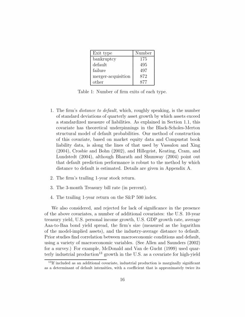
Exit type Numberbankruptcy 175default 495failure 497merger-acquisition 872other 877

Table 1: Number of firm exits of each type.

1. The firm’s distance to default, which, roughly speaking, is the numberof standard deviations of quarterly asset growth by which assets exceeda standardized measure of liabilities. As explained in Section 1.1, thiscovariate has theoretical underpinnings in the Black-Scholes-Mertonstructural model of default probabilities. Our method of constructionof this covariate, based on market equity data and Compustat bookliability data, is along the lines of that used by Vassalou and Xing(2004), Crosbie and Bohn (2002), and Hillegeist, Keating, Cram, andLundstedt (2004), although Bharath and Shumway (2004) point outthat default prediction performance is robust to the method by whichdistance to default is estimated. Details are given in Appendix A.

2. The firm’s trailing 1-year stock return.

3. The 3-month Treasury bill rate (in percent).

4. The trailing 1-year return on the S&P 500 index.

We also considered, and rejected for lack of significance in the presenceof the above covariates, a number of additional covariates: the U.S. 10-yeartreasury yield, U.S. personal income growth, U.S. GDP growth rate, averageAaa-to-Baa bond yield spread, the firm’s size (measured as the logarithmof the model-implied assets), and the industry-average distance to default.Prior studies find correlation between macroeconomic conditions and default,using a variety of macroeconomic variables. (See Allen and Saunders (2002)for a survey.) For example, McDonald and Van de Gucht (1999) used quar-terly industrial production13 growth in the U.S. as a covariate for high-yield

13If included as an additional covariate, industrial production is marginally significantas a determinant of default intensities, with a coefficient that is approximately twice its

16

bond default. Hillegeist, Keating, Cram, and Lundstedt (2004) exploit thenational rate of corporate bankruptcies in a baseline-hazard-rate model ofdefault. Fons (1991), Blume and Keim (1991), and Jonsson and Fridson(1996) document that aggregate default rates tend to be high in the down-turn of business cycles. Pesaran, Schuermann, Treutler, and Weiner (2003)use a comprehensive set of country-specific macro variables to estimate theeffect of macroeconomic shocks in one region on the credit risk of a globalloan portfolio. Keenan, Sobehart, and Hamilton (1999) and Helwege andKleiman (1997) model the forecasting of aggregate year-ahead U.S. defaultrates on corporate bonds, using, among other covariates, credit rating, ageof bond, and various macroeconomic variables, including industrial produc-tion, interest rates, trailing default rates, aggregate corporate earnings, andindicators for recession.

Firm-level earnings is a traditional predictor for bankruptcy since Altman(1968). When not appearing together with distance to default, earnings is asignificant default covariate in both logit and duration models, as shown byShumway (2001). Chava and Jarrow (2004), Bharath and Shumway (2004),Beaver, McNichols, and Rhie (2004), and Campbell, Hilscher, and Szilagyi(2005) provide additional discussion of the importance of earnings and otherfirm-specific accounting covariates.

The lack of significance of firm size as a default covariate is somewhatsurprising. For example, large firms are thought to have more financial flex-ibility than small firms. The statistical significance of size as a determinantof default risk was documented in Shumway (2001).14

3.3 Covariate Time-Series Model

We now specify a particular parameterization of the time-series model for thecovariates. Because of the extremely high-dimensional state-vector, whichincludes the macroeconomic covariates as well as the distance to default andsize of each of almost 3000 firms, we have opted for a Gaussian first-order

standard error. We did not include it as a covariate because of its marginal role andbecause of the loss in parsimony, particularly with respect to the time-series model.

14Shumway (2001), takes the size covariate to be the logarithm of the firm’s stock-marketcapitalization, relative to the total size of the NYSE and AMEX stock markets. We didnot find statistical significance, in the presence of our other covariates, of the logarithmof stock-market capitalization. (The associated standard error is approximately equal tothe coefficient estimate.)

17

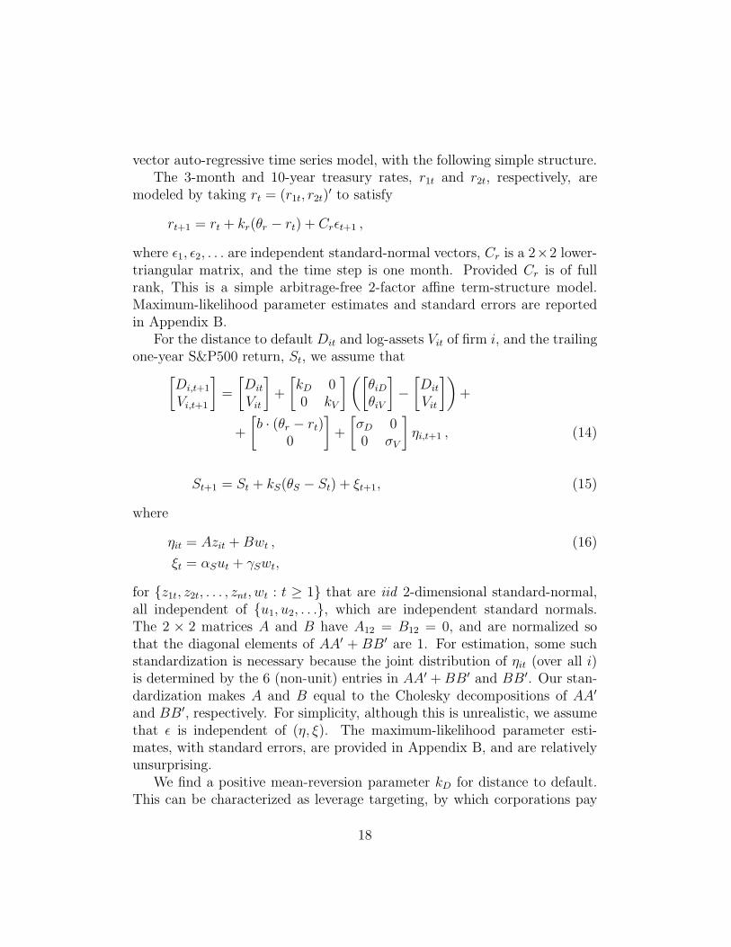
vector auto-regressive time series model, with the following simple structure.The 3-month and 10-year treasury rates, r1t and r2t, respectively, are

modeled by taking rt = (r1t, r2t)′ to satisfy

rt+1 = rt + kr(θr − rt) + Crεt+1 ,

where ε1, ε2, . . . are independent standard-normal vectors, Cr is a 2×2 lower-triangular matrix, and the time step is one month. Provided Cr is of fullrank, This is a simple arbitrage-free 2-factor affine term-structure model.Maximum-likelihood parameter estimates and standard errors are reportedin Appendix B.

For the distance to default Dit and log-assets Vit of firm i, and the trailingone-year S&P500 return, St, we assume that

[

Di,t+1

Vi,t+1

]

=

[

Dit

Vit

]

+

[

kD 00 kV

]([

θiD

θiV

]

−[

Dit

Vit

])

+

+

[

b · (θr − rt)0

]

+

[

σD 00 σV

]

ηi,t+1 , (14)

St+1 = St + kS(θS − St) + ξt+1, (15)

where

ηit = Azit +Bwt , (16)

ξt = αSut + γSwt,

for z1t, z2t, . . . , znt, wt : t ≥ 1 that are iid 2-dimensional standard-normal,all independent of u1, u2, . . ., which are independent standard normals.The 2 × 2 matrices A and B have A12 = B12 = 0, and are normalized sothat the diagonal elements of AA′ + BB′ are 1. For estimation, some suchstandardization is necessary because the joint distribution of ηit (over all i)is determined by the 6 (non-unit) entries in AA′ +BB′ and BB′. Our stan-dardization makes A and B equal to the Cholesky decompositions of AA′

and BB′, respectively. For simplicity, although this is unrealistic, we assumethat ε is independent of (η, ξ). The maximum-likelihood parameter esti-mates, with standard errors, are provided in Appendix B, and are relativelyunsurprising.

We find a positive mean-reversion parameter kD for distance to default.This can be characterized as leverage targeting, by which corporations pay

18

out dividends and other forms of distributions when they achieve a suffi-ciently low degree of leverage, and conversely attempt to raise capital andretain earnings to a higher degree when their leverage introduces financialdistress or business inflexibility, as modeled by Leland (1998) and Collin-Dufresne and Goldstein (2001). Empirical evidence of leverage targeting,allowing for delays due to frictional costs in adjusting capital structure, isprovided by Leary and Roberts (2005). It is possible that some of the esti-mated mean reversion of distance to default is due to mean reversion in assetvolatility. We assume homogeneity of kD across the sector, as we do nothave a-priori reasons to assume that different firms in the same sector revertto their targeted volatility-adjusted leverages differently from one another,and also in order to maintain a parsimonious model in the face of limitedtime-series data on each firm. (Our Monte Carlo tests confirm substantialsmall-sample bias of MLE estimators for firm-by-firm mean-reversion param-eters.) Because the distance to default is constructed by normalizing for assetvolatility, as explained in Appendix A, the Merton theory would imply thatσD does not vary across firms. In any case, we did not allow σD to vary byfirm, particularly in light of the advantages of parsimony.

A key question is how to empirically model the targeted distance to de-fault, θiD of firm i. Despite the arguments that swayed us to assume ho-mogeneity across firms of the mean-reversion and volatility parameters kD

and σD, our preliminary analysis showed that assuming a common targeteddistance to default θiD leads to estimated term structures of future defaultprobabilities that rise dramatically for firms that had consistently maintainedlow leverage during our sample period. Perhaps some firms derive reputa-tional benefits from low distress risk, or have firm-specific costs of exposureto financial distress. In the end, we opted to estimate θiD firm by firm.The median estimate of θiD across the 2770 firms in the sample is approx-imately 3.1, with an inter-quartile range of approximately 1.4 to 4.8. Thefull cross-sectional distribution of θiD and their standard errors is illustratedin Appendix B. As a long-run-mean parameter is challenging to pin downstatistically in samples of our size, however, the standard errors of our es-timates of θiD are responsible for a significant contribution to the standarderrors of our estimated term structures of default probabilities.

Even though the 10-year Treasury rate and firm size do not survive testsof statistical significance as default covariates, and are therefore excludedfrom the default intensity model, we must include them in the time-seriesmodel because they play a role in the dynamics of other variables that are

19

indeed significant as default covariates.The high-dimensional parameter search required an iterative numerical

treatment. Appendix B provides portions of the parameter estimates andstandard errors that are relevant to other calculations appearing in the paper.

3.4 Default and Other-Exit Intensities

We take the default intensities to be of the proportional-hazards form

Λ(x;µ) = eµ0+µ1x1+···+µnxn , (17)

for a covariate vector x of firm-specific and macroeconomic variables, and fora parameter vector µ = (µ0, µ1, . . . , µn) common to all firms. The other exitintensities have the same proportional-hazards form. The default intensityparameter estimates and their estimated asymptotic standard errors15 arealso reported in Table 2. The associated asymptotic covariance matrix isreported in Appendix C. For all forms of exit, the estimated standard er-rors imply statistical significance of all covariates at conventional confidencelevels, with the exception of the dependence of the merger-acquisition exitintensity on distance to default.

Consistent with the Black-Scholes-Merton model of default, estimated de-fault intensities are strongly monotonically decreasing in distance to default.For example, the parameter estimate in Table 2 reveals that a 10% reduc-tion in distance to default causes an estimated 11.3% proportional increasein default intensity. As we shall see in Section 3.5, distance to default domi-nates the other covariates in economic importance when viewed in terms ofthe impact of a typical (one-standard-deviation) variation of the covariateon the term structure of default probabilities. Figure 1 shows the empiri-cal frequency of default within one year as a function of distance to default(with kernel smoothing), indicating that the exponential dependence in (17)is at least reasonable for this crucial covariate. As illustrated, it is possiblefor distance to default to be negative. For example, a firm can exist (albeittenuously, and perhaps not for long) even with a current market value thatis smaller than the notional amount of its debt coming due in the future.

15Standard error estimates, shown in parentheses, are asymptotic standard errors ob-tained from Fisher’s information matrix, associated with (9). These asymptotic estimatesare within about 1% of bootstrap estimates of finite-sample standard errors obtained byindependent resampling firms with replacement.

20

Controlling for other covariates, the default intensity is estimated to besignificantly declining in short-term interest rates. While this runs counter tothe role of interest rates in determining the interest expense of corporations(by which higher rates place firms under more financial distress, not less),the sign of the coefficient for the short rate is consistent with the fact thatshort rates are often increased by the U.S. Federal Reserve in order to “cooldown” business expansions. Default intensities are estimated to increase inthe trailing one-year return of the S&P 500, controlling for other covariates.This could be due to correlation between individual stock returns and S&P500 stock returns, and perhaps the trailing nature of the returns and business-cycle dynamics.

Exit type constant DTD return 3-mo. r SPXbankruptcy −3.099 −1.089 −0.930 −0.153 1.074

(0.198) (0.062) (0.141) (0.037) (0.489)

default −2.156 −1.129 −0.694 −0.105 1.203(0.113) (0.036) (0.075) (0.021) (0.289)

failure −2.148 −1.129 −0.692 −0.106 1.185(0.113) (0.036) (0.074) (0.021) (0.289)

merger −3.220 0.021 0.310 −0.137 1.442(0.098) (0.013) (0.050) (0.014) (0.241)

other −2.773 −0.072 0.677 −0.167 0.674(0.095) (0.014) (0.040) (0.015) (0.231)

Table 2: Maximum likelihood estimates of intensity parameters, with parenthetic stan-dard errors. “DTD” is distance to default, “return” is the trailing one-year stock returnof the firm, “3-mo. r” is the current 3-month treasury rate, and “SPX” is the trailingone-year return of the S& P 500.

As a rough diagnostic of the reasonableness of the overall fit of the model,one can compare the total predicted number of defaults implied by the esti-mated default intensity paths, about 471 (which is the integral of the totaldefault intensity path shown in Figure 2), with the actual number of de-faults during the same period, 495. The out-of-sample predictive power ofthe estimated model is reviewed in Section 4.

21

−0.5 0 0.5 1 1.5 2 2.5 3 3.5 4 4.5 5−0.01

0

0.01

0.02

0.03

0.04

0.05

Distance to default

Fre

quen

cyof

def

ault

wit

hin

one

year

Figure 1: The dependence of empirical default frequency on distance to default.

3.5 Term Structures of Default Hazards

We are now in a position to obtain maximum-likelihood estimates, by firmand conditioning date, of the term structure of conditional default probabil-ities. These are obtained from their theoretical counterparts by substitutingparameter estimates into (1). In order to illustrate the results more meaning-fully, we will report examples of the estimated probability density qs(Xit, s)(the partial derivative of q( · ) with respect to time horizon s) of the defaulttime,16 and the estimated default hazard rate

H(Xit, s) =qs(Xit, s)

p(Xit, s), (18)

16This density is most easily calculated by differentiation through the expectation, as

E(

e−R

t+s

t[λ(u)+α(u)] duλ(t + s) |Xt

)

, which we compute by Monte-Carlo simulation. We

emphasize that this density is “improper” (integrates over all s to less than one) becauseof nondefault exit events.

22

1975 1980 1985 1990 1995 2000 20050

10

20

30

40

50

60

70

80

Def

ault

san

ddef

ault

inte

nsi

ty

Year

Figure 2: The total across firms of default intensities (line), and the number of defaultsin each year (bars), 1979-2004.

where p(Xit, s) is the estimated survival probability, from (2). The hazardrate H(Xit, s) is mean rate of arrival of default at time t+ s, conditioning onthe covariate vector Xit at time t, and conditioning as well on the event ofsurvival up until time t + s. We emphasize that this default hazard rate attime horizon s conditions on survival to time s from both default and fromother forms of exit.17 If the intensity of default and the intensity of otherforms of exit are independent processes, then controlling for survivorshipfrom other forms of exit has no effect on the default hazard rate. In our case,the default intensity and other-exit intensity are correlated since they dependon the same covariates, however the effect of this correlation on the defaulthazard rates is small. In our illustrative calculations, we account for theother-exit effects associated with merger and acquisition, viewing the otherforms of exit as less relevant in practical terms for avoiding default. Even

17The total-exit hazard rate is, notationally suppressing all arguments of the survivalfunction p( · ) except for the time horizon s, given as usual by −ps(s)/p(s).

23

a merger or acquisition need not prevent the future default of a particulardebt instrument (depending, for example, on whether that debt instrumentis paid down immediately, assumed by the new corporation, or exchangedfor a new form of debt issued by the new corporation), although of course anacquisition rules out a future bankruptcy by the acquired firm itself.

0 0.5 1 1.5 2 2.5 3 3.5 40

100

200

300

400

500

600

Haz

ard

rate

(bas

ispoi

nts

)

Years ahead

Figure 3: Annualized Xerox default hazard rates as of January 1, 2001 (solid curve),with one-standard-error bands associated with parameter uncertainty (dotted curves).

We consider Xerox as an illustrative firm, and take January 1, 2000 as theconditioning date t. The estimated term structure of Xerox’s default hazardrates as of that date is shown in Figure 3. The asymptotic one-standard-errorbands of the estimated hazard rates associated with parameter uncertaintyare shown with dashed lines, and are obtained by the usual “Delta method,”as explained in Appendix C.

The estimated term structure of default hazard rates shown in Figure 3is downward-sloping mainly because Xerox’s distance to default, 0.95, waswell below its estimated target, θiD = 4.4 (which has an estimated standarderror of 1.4). Other indications that Xerox was in signficant financial distress

24

at this point were its 5-year default swap rate of 980 basis points18 and itstrailing 1-year stock return19 of −71%.

0 0.5 1 1.5 2 2.5 3 3.5 40

500

1000

1500

2000

2500

Years ahead

Ann

ualiz

ed h

azar

d ra

te (

basi

s po

ints

)

Figure 4: Annualized Xerox default hazard rates as of January 1, 2000 (solid curve),and with distance to default at one standard deviation (1.33) below its current level of0.95 (dotted curve), and with distance to default at one standard deviation above currentlevel (dashed curve). The trailing S& P 500 return was −8.6%, the trailing one-year stockreturn of Xerox was −71%, the 3-month treasury rate was 5.8%, and the 10-year treasuryyield was 5.2%.

Figure 4 shows the hypothetical effects on the term structure of Xerox’sdefault hazard rates of one-standard-deviation shifts (from its stationary dis-tribution) of its distance to default, above or below its current level.20 Interms of both the impact of normalized shocks to default intensity as well

18This CDS rate is an average of quotes provided from GFI and Lombard Risk.19As an intensity covariate, the trailing-stock-return covariate is measured on a contin-

uously compounding basis, and was −124%.20For example, with a mean-reversion parameter of κY and an innovation standard

deviation of σY , the stationary distribution of a first-order autoregressive process Y has astandard deviation whose maximum likelihood estimate is dY = σ2

Y/(1 − (1 − κY )2).

25

0 0.5 1 1.5 2 2.5 3 3.5 40

100

200

300

400

500

600

700

Years ahead

Ann

ualiz

ed h

azar

d ra

te (

basi

s po

ints

)

Figure 5: Annualized Xerox default hazard rates as of January 1, 2000 (solid curve), andwith the 3-month treasury rate at one standard deviation (3.6%) below the current levelof 5.8% (dotted curve), and at one standard deviation above the current level (dashedcurve).

time-series presistence, shocks to distance to default have a relatively greatereffect on the term structure of Xerox’s default hazard rates than do similarlysignificant shocks to any of the other covariates. Figure 5, for example, showsthe analogous effects of a one-standard-deviation shock (from its stationarydistribution) to the current short-term interest rate. The effect of such a shiftin interest rates has a smaller effect than the effect of the analogous shift toXerox’s distance to default, both because of the relative sizes of these shocks,as scaled by the corresponding intensity coefficients, and also because inter-est rates are less persistent (have a higher mean-reversion rate) than distanceto default.

By the beginning of 2004, Xerox’s term structure of hazard rates hadshrunk dramatically to that shown in Figure 6, mainly because its distance

26

0 1 2 3 4 5 6 7 80

10

20

30

40

50

60

70

Years ahead

Ann

ualiz

ed h

azar

d ra

te (

basi

s po

ints

)

Figure 6: Annualized Xerox default hazard rates as of January 1, 2004 (solid curve),and with distance to default at one standard deviation (1.33) below its current level of 3.7(dotted curve), and with distance to default at one standard deviation above current level(dashed curve).

to default had grown to 3.7. The short-maturity hazard rates were also re-duced by Xerox’s high trailing one-year stock return of21 +95%. The shape ofthe term structure of hazard rates is also influenced by the non-linear depen-dence of the covariate-conditional default probabilities on future covariatescombined with uncertainty over these future covariates. For example, theterm structure of hazard rates can be upward sloping even when the initialcovariates are at their long-run means. There are two opposing “convexity”effects here, both due to Jensen’s Inequality. First, the intensities are convexwith respect to the covariates, so the expected future intensities are higherthan the intensities evaluated at the expected covariates. Second, the condi-tional survival probabilities are convex with respect to the path of intensities,so the survival probablities are higher (and default probabilities are lower)

21On a continuously-compounding basis, the trailing one-year return was 67%.

27

than they would be when evaluated at the expected path of the intensities.These competing effects are not canceling.

Figure 7 shows the estimated conditional probability density function ofXerox’s default time as of January 1, 2004, and how much larger this default-time density would be if one were to ignore the effect of merger and acquisi-tion (that is, if one assumes that the merger-acquisition intensity parametervector ν is zero). For example, Xerox obviously cannot itself fail more thanone year into the future in the event that it is merged with another firm inless than one year.

0 1 2 3 4 5 6 7 81.2

1.4

1.6

1.8

2

2.2

2.4

2.6

2.8

3x 10

−3

Def

ault

tim

elike

lihood

Years ahead

Figure 7: Estimated conditional density of Xerox’s default time as of January 1, 2001.Bottom plot: the estimated default time density, incorporating the impact of survival frommerger and acquisition. Top plot: the estimated default-time density obtained by ignoring(setting to zero) the intensity of other exits.

As illustrated above, the shapes of the term structure of Xerox’s condi-tional default hazard rates for future years reflects the time-series dynamicsof the covariates. The counter-cyclical behavior of default probabilities is al-ready well documented in such prior studies as Fons (1991), Blume and Keim(1991), Jonsson and Fridson (1996), McDonald and Van de Gucht (1999),

28

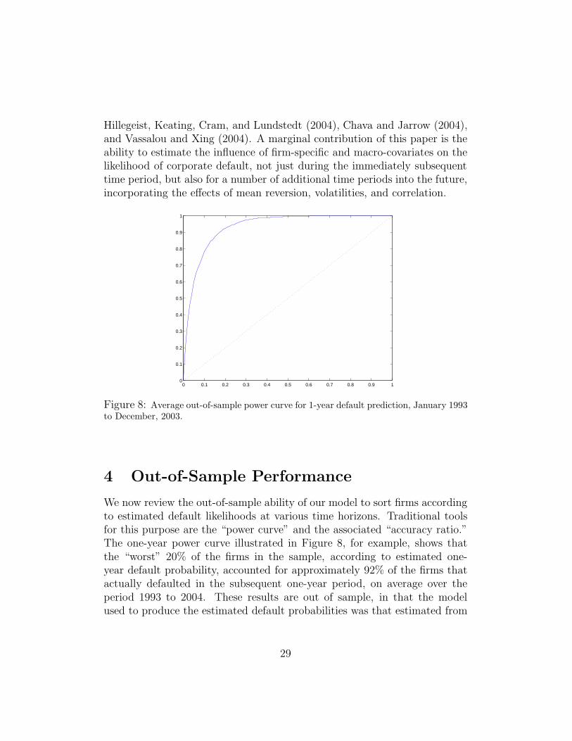
Hillegeist, Keating, Cram, and Lundstedt (2004), Chava and Jarrow (2004),and Vassalou and Xing (2004). A marginal contribution of this paper is theability to estimate the influence of firm-specific and macro-covariates on thelikelihood of corporate default, not just during the immediately subsequenttime period, but also for a number of additional time periods into the future,incorporating the effects of mean reversion, volatilities, and correlation.

0 0.1 0.2 0.3 0.4 0.5 0.6 0.7 0.8 0.9 10

0.1

0.2

0.3

0.4

0.5

0.6

0.7

0.8

0.9

1

Figure 8: Average out-of-sample power curve for 1-year default prediction, January 1993to December, 2003.

4 Out-of-Sample Performance

We now review the out-of-sample ability of our model to sort firms accordingto estimated default likelihoods at various time horizons. Traditional toolsfor this purpose are the “power curve” and the associated “accuracy ratio.”The one-year power curve illustrated in Figure 8, for example, shows thatthe “worst” 20% of the firms in the sample, according to estimated one-year default probability, accounted for approximately 92% of the firms thatactually defaulted in the subsequent one-year period, on average over theperiod 1993 to 2004. These results are out of sample, in that the modelused to produce the estimated default probabilities was that estimated from

29

data for 1979 to the end of 1992. Figure 9 provides the analogous results for5-year-ahead prediction, for 1993 to 2000.

0 0.1 0.2 0.3 0.4 0.5 0.6 0.7 0.8 0.9 10

0.1

0.2

0.3

0.4

0.5

0.6

0.7

0.8

0.9

1

Figure 9: Average out-of-sample power curve for 5-year default prediction, January 1993to December, 1999.

The accuracy ratio associated with a given power curve is defined to betwice the area between the power curve and the 45-degree line. (The maxi-mum possible accuracy ratio is therefore below 100% by the sample averageof the annual default rate.) Table 3 shows average 1-year and average 5-year accuracy ratios for each of the exit types considered, over the post-1993sample periods. Notably, the accuracy ratios are essentially unchanged whenreplacing the model as estimated in 1993 with the sequence of models es-timated at the beginnings of each of the respective forecast periods. Theone-year-ahead out-of-sample accuracy ratio for default prediction from ourmodel, over 1993-2003, is 88%. Hamilton and Cantor (2004) report that,for 1999-2003, the average accuracy ratio for default prediction based onMoody’s credit ratings22 is 65%, while those based on ratings adjustmentsfor placements on Watchlist and Outlook are 69%, and those based on sort-ing firms by bond yield spreads average 74%. On average over 1983-2005,

22Kramer and Guttler (2003) report no statistically significant difference between theaccuracy ratio of Moodys and Standard-and-Poors ratings in a sample of 1927 borrowers.

30

Moody’s reported23 a substantially higher average 1-year acuracy ratio of84.6%.

The out-of-sample accuracy for prediction of merger and acquisition isnegative, indicating no out-of-sample power to discriminate among firms re-garding their likelihood of being merged or acquired. (Randomly sorting thefirms would produce an accuracy ratio, in a large sample, of approximatelyzero.) Putting aside the failure of our model to predict merger or acquisition,this implies that the model-implied probabilities of avoiding default througha prior merger event, as depicted in Figure 7, although roughly accurateon average over our firms and historical data, are unlikely to be meaningfulwhen comparing across different firms or different points in time.

AR1 AR5bankruptcy 0.88 0.69default 0.87 0.70failure 0.86 0.70merger −0.03 −0.01other exit 0.19 0.11

Table 3: Out-of-sample average accuracy ratios, 1993 to 2004 for 1-year prediction, and1993 to 2000 for 5-year prediction.

Figures 10 and 11 show the time series of the accuracy ratios for 1-year-out and 5-year-out default prediction throughout the out-of-sample period.

Bharath and Shumway (2004) analyze out-of-sample predictive perfor-mance in terms of the average (over quarters) of the fraction of firms in theirsample that default in the subsequent quarter that were sorted by the modelinto the lowest-quality decile of firms at the beginning of the quarter. For ex-ample, for a particular sample, during the period 1991-2003, they report thatsorting based on KMV EDFs places approximately 69% of the quarter-aheaddefaulting firms in the lowest decile. Sorting based on the more elaboratemodels developed by Bharath and Shumway (2004) places approximately77% in the lowest decile. For our own sample and the period 1993-2004, thisaccuracy measure rises to 94%.

23See “The Performance of Moody’s Corporate Bond Ratings: June 2005, QuarterlyUpdate,” Moody’s Investors Services Special Comment, July 2005.

31

1993 1994 1995 1996 1997 1998 1999 2000 2001 2002 2003 2004−0.2

0

0.2

0.4

0.6

0.8

1

Figure 10: One-year accuracy ratios. Dashed line: bankruptcy. Solid line: default.Dotted line: other exit. Broken dash-dot line: merger.

1993 1994 1995 1996 1997 1998 1999 2000−0.1

0

0.1

0.2

0.3

0.4

0.5

0.6

0.7

0.8

0.9

Figure 11: Five-year accuracy ratios. Dashed line: bankruptcy. Solid line: default.Dotted line: other exit. Broken dash-dot line: merger.

The model of Beaver, McNichols, and Rhie (2004) based on accountingratios places 80.3% of the year-ahead defaulters in the lowest two deciles, outof sample, for the period 1994-2002. Consistent with the important role of

32

market variables discovered by Shumway (2001), when Beaver, McNichols,and Rhie (2004) add stock-market variables in combination with accountingratios, this measure goes up to 88.1%, and when they further allow theirmodel coefficients to adjust over time, this measure rises to 92%, which isroughly the measure obtained for our model and data.

5 Concluding Remarks

This paper offers an econometric method for estimating term structures ofcorporate default probabilities over multiple future periods, conditional onfirm-specific and macroeconomic covariates. We also provide an empirical im-plementation of this method for the U.S.-listed Industrial firms. The method,under its assumptions, allows one to combine traditional duration analysisof the dependence of event intensities on time-varying covariates with con-ventional time-series analysis of covariates, in order to obtain maximum-likelihood estimation of multi-period survival probabilities.

Applying this method to data on U.S.-listed Industrial firms over 1979to 2004, we find that the estimated term structures of default hazard ratesof individual firms in this sector depend significantly, in level and shape, onthe current state of the economy, and especially on the current leverage ofthe firm, as captured by distance to default, a volatility-adjusted leveragemeasure that is popular in the banking industry.

Our methodology could be applied to other settings involving the forecast-ing of discrete events over multiple future periods, in which the time-seriesbehavior of covariates could play a significant role, for example: mortgageprepayment and default, consumer default, initial and seasoned equity offer-ings, merger, acquisition, and the exercise of real timing options, such as theoption to change or abandon a technology. (We have shown, however, thatdifferent covariates or time-series specifications would be needed in order toaccurately predict merger or acquisitions.)

Our methodology also allows estimates of portfolio credit risk, as it pro-vides maximum-likelihood estimates of joint probabilities of default. For agiven maturity T , the default-event correlation between firms i and j is thecorrelation between the random variables 1τ(i)<T and 1τ(j)<T. These cor-relations can be calculated by using the fact that, in a doubly-stochasticframework, for stopping times τ(A) and τ(B) that are the first jump timesof counting processes with respective intensities λA and λB, the probability

33

of joint survival to time T is

E(1τ(A)>T1τ(B)>T) = P (τ(A) > T, τ(B) > T ) = E(

e−R

T

0(λA(t)+λB(t)) dt

)

.

Unfortunately, our estimated model implies unrealistically low estimates ofdefault correlation, compared to the sample correlations reported by DeServi-gny and Renault (2002). This is a topic of separate ongoing research.

We conclude by comparing our model with that of structural models ofdefault, for example Merton (1974). The main distinctions between the twomodeling approaches are the nature of the event that triggers default, andof course the empirical fit. Our assumptions about the asset process anddistance-to-default process include those of the Merton model as a specialcase, and would be identical to those of the Merton model if we take theparticular case of no leverage targeting. That is, removing mean reversion,our distance to default process is a Brownian motion, just as in Merton(1974), and our asset process is a geometric Brownian motion, just as inMerton. With regard to what triggers default, our model is quite differentfrom structural models, including Merton (1974) as well as first-passage struc-tural models, such as those of Fisher, Heinkel, and Zechner (1989) and Leland(1994). The structural models apply a solvency test, regarding whether thedistance to default falls below some barrier, that is in some cases determinedendogenously. Our model assumes instead that, at each “small” time pe-riod, default occurs (or not) at random, with a probability that depends onthe current distance to default and other explanatory variables. It is known(for example, Duffie and Lando (2001)) that these structural models producehighly unrealistically shaped term structures of default probabilities, giventhe continuity properties of Brownian motion and the undue precision withwhich distance to default is assumed to be measured. In particular, the as-sociated default probabilities are extremely small for maturities of roughlytwo years or less (at typical parameters), even for low-quality firms. Exten-sions of these structural models with imperfectly observed leverage (or withsignificant jumps in leverage) and with leverage targeting (as suggested byCollin-Dufresne and Goldstein (2001)) would have more realistic term struc-tures of default probabilities. Theory as well as our empirical results suggestthat enriching structural models with additional state variables (beyond thedistance to default), such as macro-economic variables, could lead to an im-provement for such extended structural models. The evidence that we havepresented here may provide some clues for future research in this direction.

34

Appendices

A Construction of Distance to Default

This appendix explains how we construct the distance to default covariate,following a recipe similar to those of Vassalou and Xing (2004), Crosbie andBohn (2002), Hillegeist, Keating, Cram, and Lundstedt (2004), and Bharathand Shumway (2004). For a given firm, the distance to default is, roughlyspeaking, the number of standard deviations of asset growth by which a firm’smarket value of assets exceeds a liability measure. Formally, for a given firmat time t, the distance to default is

Dt =ln(

Vt

Lt

)

+(

µA − 12σ2

A

)

T

σA

√T

, (19)

where Vt is the market value of the firm’s assets at time t and Lt is a liabilitymeasure, defined below, that is often known in industry practice as the “de-fault point.” Here, µA and σA measure the firm’s mean rate of asset growthand asset volatility, respectively, and T is a chosen time horizon, typicallytaken to be 4 quarters.

The default point Lt, following the standard established by Moodys KMV(see Crosbie and Bohn (2002), as followed by Vassalou and Xing (2004)), ismeasured as the firm’s book measure of short-term debt, plus one half ofits long-term debt (Compustat item 51), based on its quarterly accountingbalance sheet. We have measured short term debt as the larger of Compustatitems 45 (“Debt in current liabilities”), and 49 (“Total Current Liabilities”).If these accounting measures of debt are missing in the Compustat quarterlyfile, but available in the annual file, we replace the missing data with theassociated annual debt data.

We estimate the assets Vt and volatility σA according to a call-optionpricing formula, following the theory of Merton (1974) and Black and Scholes(1973), under which equity may be viewed as a call option on the value of afirm’s assets, Vt. In this setting, the market value of equity, Wt, is the optionprice at strike Lt and time T to expiration.

We take the initial asset value Vt to be the sum of Wt (end-of-quarterstock price times number of shares outstanding, from the CRSP database)

35

and the book value of total debt (the sum of short-term debt and long-termdebt from Compustat). We take the risk-free return r to be the one-year T-bill rate. We solve for the asset value Vt and asset volatility σA by iterativelyapplying the equations:

Wt = VtΦ(d1) − Lte−rT Φ(d2) (20)

σA = sdev (ln(Vt) − ln(Vt−1)) , (21)

where

d1 =ln(

Vt

Lt

)

+ (r + 12σ2

A)T

σA

√T

, (22)

d2 = d1 − σA

√T , and Φ( · ) is the standard-normal cumulative distribution

function, and sdev( · ) denotes sample standard deviation. Equation (20) is avariant of the call-option pricing formula of Black and Scholes (1973), allow-ing, through (21), an estimate of the asset volatility σA. For simplicity, byusing (21), we avoided the calculation of the volatility implied by the optionpricing model (as in Crosbie and Bohn (2002) and Hillegeist, Keating, Cram,and Lundstedt (2004)), but instead estimated σA as the sample standarddeviation of the time series of quarterly asset-value growth, ln(Vt)− ln(Vt−1).

B Time-Series Parameter Estimates

For the 2-factor interest rate model parameters, our maximum likelihoodparameter estimates, with standard errors in subscripted parentheses, are

kr =

(

0.03 (0.026) −0.021 (0.030)

−0.027 (0.012) 0.034 (0.014)

)

,

θr =

(

3.59 (4.08)

5.47 (3.59)

)

,

and

Cr =

(

0.5639 (0.035) 00.2247 (0.026) 0.2821 (0.008)

)

,

where θr is measured in percentage points.

36

Joint maximum likelihood estimation of equations (14), (15), and (16),simultaneously across all firms i in 1, . . . , n gives the parameter estimates(with standard errors in subscripted parentheses):

b =(

0.0090(0.0021) −0.0121(0.0024)

)′

kD =0.0355(0.0003)

σD =0.346(0.0008)

kv =0.015(0.0002)

σv =0.1169(0.0002)

AA′ +BB′ =

(

1 0.448(0.0023)

0.448(0.0023) 1

)

BB′ =

(

0.0488(0.0038) 0.0338(0.0032)

0.0338(0.0032) 0.0417(0.0033)

)

kS =0.1137(0.018)

αS =0.047(0.0019)

θS =0.1076(0.0085)

γS =(

0.0366(0.0032) 0.0134(0.0028)

)

.′

Figure 12 shows the cross-sectional distribution of estimated targeteddistance to default, θiD, with standard errors. While some firms are estimatedto target negative distances to default, which is not contrary to theory, thisis likely to be an unfortunate artifact of the model specification. One couldinstead constrain the parameter θiD to be non-negative.

37

0 500 1000 1500 2000 2500

−6

−4

−2

0

2

4

6

8

10

12

14E

stim

ate

ofθ i

D

Rank of firm

Figure 12: Cross-sectional distribution of estimated targeted distance to default, θiD,sorted, with (vertically) one-standard-error bands for each.

C Delta-based Standard Errors

The confidence intervals plotted in Figure 3 are asymptotic standard errorsobtained from the Delta method. For this, we require an estimate of thecovariance matrix Σ of the MLE estimator ψi of the portion of the parametervector ψi affecting the hazard rates of firm i, which in this case is Xerox. Welet ψi = (γi, µ, ν), where γi is the vector of parameters of the time-seriesmodel for Xit, and where µ and ν parameterize the default and other-exitintensities, respectively, as in Section 2.

Fixing Xit = (Dit, Vit, St, rt) and the time horizon s, we write

H(Xit, s;ψi) = G(ψi). (23)

The default probability q(Xit, s;ψi), default-time density qs(Xit, s;ψi),

38

survival probability p(Xit, s;ψi), and default hazard rate H(Xit, s;ψi) are allcontinuous with respect to the parameter vector ψi, by the dominated con-vergence theorem, using the fact that e−

R

t+s

t[λ(u)+α(u)] du is strictly positive

and bounded by 1, using the continuity of the probability distribution of thecovariate process with respect to the parameters, using the monotonicity ofthe default and other-exit time intensities with respect to the parameters,and finally using the fact that λ(t + s) is the double-exponential of a nor-mal variable. Thus, under the consistency assumption that ψi converges indistribution with sample size to ψi, the continuity of G( · ) implies that themaximum-likelihood estimator G(ψi) of G(ψi) is also consistent. Moreover,with the addition of differentiability and other technical conditions, G(ψi)has the asymptotic variance estimate ∇G(ψi)Σ∇G(ψi)

′, where ∇G( · ) is thegradient of G and where

Σ =

Σγi0

Σµ

0 Σν

(24)

is determined by the asymptotic covariance matrices Σγi, Σµ, and Σν of γi, µ,

and ν, respectively. These asymptotic covariance matrices are obtained bythe usual method of inverting the Hessian matrix of the likelihood functions,evaluated at the parameter estimates.

For example, the asymptotic estimate of the covariance matrix of theMLE estimators of the default intensity parameters (µ0, µ2, µ1, µ2, µ3, µ4),corresponding to the constant, distance to default, same-firm trailing stockreturn, 3-month Treasury rate, and trailing S& P 500 return, respectively, is

Σµ =

0.0128 0.0004 0.0029 −0.0019 0.00340.0004 0.0013 −0.0011 −0.0001 −0.00150.0029 −0.0011 0.0056 −0.0000 −0.0025−0.0019 −0.0001 −0.0000 0.0004 −0.00220.0034 −0.0015 −0.0025 −0.0022 0.0836

. (25)

39

References

Allen, L. and A. Saunders (2002). A Survey of Cyclical Effects in CreditRisk Measurement Models. mimeo, Stern School of Business, New YorkUniversity.

Altman, E. I. (1968). Financial Ratios, Discriminant Analysis, and thePrediction of Corporate Bankruptcy. Journal of Finance 23, 589–609.

Amemiya, T. (1985). Advanced Econometrics. Cambridge, Massachusetts:Harvard University Press.

Andersen, P. K., O. Borgan, R. D. Gill, and N. Keiding (1992). StatisticalModels Based on Counting Processes. New York: Springer-Verlag.

Beaver, B. (1966). Financial Ratios as Predictors of Failure. EmpiricalResearch in Accounting: Selected Studies, Supplment to Journal of Ac-counting Research Autumn, 91–101.

Beaver, B. (1968a). Alternative Accounting Measures as Predictors of Fail-ure. Accounting Review January, 113–122.

Beaver, B. (1968b). Market Prices, Financial Ratios, and the Predictionof Failure. Journal of Accounting Research Autumn, 170–192.

Beaver, W., M. McNichols, and J.-W. Rhie (2004). Have Financial State-ments Become Less Informative? — Evidence from the Ability of Fi-nancial Ratios to Predict Bankruptcy. Working Paper, Stanford Uni-versity.

Behar, R. and K. Nagpal (1999). Dynamics of Rating Transition. WorkingPaper, Standard and Poor’s.

Berman, S. M. and H. Frydman (1999). Parametric Estimation of HazardFunctions with Stochastic Covariate Processes. Sankhya, Series A 61,174–188.

Bharath, S. and T. Shumway (2004). Forecasting Default with the KMV-Merton Model. Working Paper, University of Michigan.

Black, F. and M. Scholes (1973). The Pricing of Options and CorporateLiabilities. Journal of Political Economy 81, 637–654.

Blume, M. and D. Keim (1991). Realized Returns and Volatility of Low-Grade Bonds: 1977-1989. Journal of Finance 46, 49–74.

40

Campbell, J., J. Hilscher, and J. Szilagyi (2005). In Search of DistressRisk. Working Paper, Harvard University.

Carty, L. (2000). Corporate Credit Risk Dynamics. Financial AnalystsJournal , 67–81, July–August.

Chava, S. and R. Jarrow (2004). Bankruptcy Prediction with IndustryEffects. Review of Finance 8, 537–569.

Collin-Dufresne, P. and R. Goldstein (2001). Do Credit Spreads ReflectStationary Leverage Ratios? Reconciling Structural and Reduced-Form Frameworks. Journal of Finance 56, 1929–1958.

Cox, D. R. and V. Isham (1980). Point Processes. New York: Chapmanand Hall.

Cox, D. R. and D. Oakes (1984). Analysis of Survival Data. New York:Chapman and Hall.

Crosbie, P. J. and J. R. Bohn (2002). Modeling Default Risk. TechnicalReport, KMV, LLC.

Daley, D. J. and D. Vere-Jones (1988). An Introduction to the Theory ofPoint Processes. New York: Springer.

Das, S. R., D. Duffie, N. Kapadia, and L. Saita (2005). Common Failings:How Corporate Defaults are Correlated. Working Paper, Stanford Uni-versity, forthcoming, Journal of Finance.

DeServigny, A. and O. Renault (2002). Default Correlation: EmpiricalEvidence. Working Paper, Standard and Poor’s.

Duffie, D. (2001). Dynamic Asset Pricing Theory (Third edition). Prince-ton, New Jersey: Princeton University Press.

Duffie, D. and D. Lando (2001). Term Structures of Credit Spreads withIncomplete Accounting Information. Econometrica 69, 633–664.

Engle, R. F. and J. R. Russell (1998). Autoregressive Conditional Dura-tion: A New Model for Irregularly Spaced Transaction Data. Econo-metrica 66, 1127–1162.

Fisher, E., R. Heinkel, and J. Zechner (1989). Dynamic Capital StructureChoice: Theory and Tests. Journal of Finance 44, 19–40.

Fons, J. (1991). An Approach to Forecasting Default Rates. Working Pa-per, Moody’s Investors Services.

41

Hamilton, D. and R. Cantor (2004). Ratings Transitions and Default RatesConditionaed on Outlooks. The Journal of Fixed Income, September,54–70.

Helwege, J. and P. Kleiman (1997). Understanding Aggregate DefaultRates of High Yield Bonds. Journal of Fixed Income 7, 55–62.

Hillegeist, S. A., E. K. Keating, D. P. Cram, and K. G. Lundstedt (2004).Assessing the Probability of Bankruptcy. Review of Accounting Stud-ies 9, 5–34.

Jones, F. (1987). Current Techniques in Bankruptcy Prediction. Journalof Accounting Literature 6, 131–164.

Jonsson, J. and M. Fridson (1996, June). Forecasting Default Rates onHigh-Yield Bonds. The Journal of Fixed Income, 69–77.

Kalbfleisch, J. and R. Prentice (2002). The Statistical Analysis of FailureTime Data (Second edition). Hoboken, New Jersey: John Wiley &Sons.

Karr, A. (1991). Point Processes and Statistical Inference (Second edition).New York: Marcel Dekker.

Kavvathas, D. (2001). Estimating Credit Rating Transition Probabilitiesfor Corporate Bonds. Working paper, University of Chicago.

Kealhofer, S. (2003). Quantifying Credit Risk I: Default Prediction. Fi-nancial Analysts Journal , January–February, 30–44.

Keenan, S. C., J. Sobehart, and D. T. Hamilton (1999). Predicting DefaultRates: A Forecasting Model For Moody’s Issuer-Based Default Rates.Working Paper, Moody’s Investors Services.

Kramer, W. and A. Guttler (2003). Comparing the Accuracy of DefaultPredictions in the Ratings Industry: The Case of Moody’s vs. S& P.Working Paper, Statistics Department, University of Dortmund.

Lancaster, T. (1990). The Econometric Analysis of Transition Data. NewYork: Cambridge University Press.

Lando, D. and T. Skødeberg (2002). Analyzing Rating Transitions andRating Drift with Continuous Observations. Journal of Banking andFinance 26, 423–444.

42

Lane, W. R., S. W. Looney, and J. W. Wansley (1986). An Applicationof the Cox Proportional Hazards Model to Bank Failure. Journal ofBanking and Finance 10, 511–531.

Leary, M. and M. Roberts (2005). Do Firms Rebalance their Capital Struc-tures? Journal of Finance 60, 2575–2620.

Lee, S. H. and J. L. Urrutia (1996). Analysis and Prediction of Insolvencyin the Property-Liability Insurance Industry: A Comparison of Logitand Hazard Models. The Journal of Risk and Insurance 63, 121–130.

Leland, H. (1994). Corporate Debt Value, Bond Covenants, and OptimalCapital Structure. Journal of Finance 49, 1213–1252.

Leland, H. (1998). Agency Costs, Risk Manamgement, and Capital Struc-ture. Journal of Finance 53, 1213–1242.

McDonald, C. G. and L. M. Van de Gucht (1999). High-Yield Bond Defaultand Call Risks. Review of Economics and Statistics 81, 409–419.

Merton, R. C. (1974). On the Pricing of Corporate Debt: The Risk Struc-ture of Interest Rates. Journal of Finance 29, 449–470.

Meyer, B. D. (1990). Unemployment Insurance and Unemployment Spells.Econometrica 58, 757–782.

Miller, R. (1981). Survival Analysis. New York: John Wiley & Sons.

Nickell, P., W. Perraudin, and S. Varotto (2000). Stability of Rating Tran-sitions. Journal of Banking and Finance 24, 203–227.

Ohlson, J. (1980). Financial Ratios and the Probabilistic Prediction ofBankruptcy. Journal of Accounting Research 19, 109–131.

Pesaran, M. H., T. Schuermann, B.-J. Treutler, and S. M. Weiner (2003).Macroeconomic Dynamics and Credit Risk: A Global Perspective.Working paper. Wharton School, Federal Reserve Bank, New York,forthcoming in Journal of Money, Credit, and Banking.

Philosophov, L. and V. Philiosophov (2002). Corporate Bankruptcy Prog-nosis: An Attempt at a Combined Prediction of the Bankruptcy Eventand Time Interval of its Occurrence. International Review of FinancialAnalysis 11, 375–406.

Protter, P. (1990). Stochastic Integration and Differential Equations. NewYork: Springer-Verlag.

43

Shumway, T. (2001). Forecasting Bankruptcy More Accurately: A SimpleHazard Model. Journal of Business 74, 101–124.

Therneau, T. M. and P. M. Grambsch (2000). Modeling Survival Data:Extending the Cox Model. New York: Springer-Verlag.

Vassalou, M. and Y. Xing (2004). Default Risk in Equity Returns. Journalof Finance 59, 831–868.

Whalen, G. (1991). A Proportional Hazards Model of Bank Failure: AnExamination of its Usefulness as an Early Warning Model Tool. InFederal Reserve Bank of Cleveland Economic Review, pp. 21–31. 1991.

Wheelock, D. C. and P. W. Wilson (2000). Why Do Banks Disappear?The Determinants of U.S. Bank Failures and Acquisitions. Review ofEconomics and Statistics 82, 127–138.

Wilson, T. (1997a). Portfolio Credit Risk, I. RISK 10, September, 111–117.

Wilson, T. (1997b). Portfolio Credit Risk, I. RISK 10, October, 56–61.

44