NBER WORKING PAPER SERIES

MONEY, REAL INTEREST RATES, AND OUTPUT:A REINTERPRETATION OF POSTWAR U.S. DATA

Robert B. Litterman

Laurence Weiss

Working Paper No. 1077

NATIONAL BUREAU OF ECONOMIC RESEARCH1050 Massachusetts Avenue

Cambridge MA 02138

February 1983

Federal Reserve Bank of Minneapolis and University of Chicago,

respectively. Financial support from NSF grant SES-8026587 is gra-tefully acknowledged. Work on this paper was initiated in 1980 atthe Massachusetts Institute of Techno1or where Litterman was anassistant professor and Weiss was visiting. We are indebted to toomany of our colleagues to enumerate for their insights andsuggestions in the course of writing this paper. In particular,though, we wish to thank Christopher Sims, Stanley Fischer, RobertHall, Robert Shiller, James Tobin, and P.C.B. Phillips. Theresearch reported here is part of the NBER's research program inEconomic Fluctuations. Any opinions expressed are those of theauthors and not those of the National Bureau of Economic Research.

NBER Working Paper #1077February 1983

Money, Real Interest Rates, and Output:A Reinterpretation of Postwar U.S. Data

ABSTRACT

This paper reexamines both monthly and quarterly U.S. postwar data

to investigate if the observed comovements between money, real interest

rates, prices and output are compatible with the money——real interest——output

link suggested by existing monetary theories of output, which include

both Keynesian and equilibrium models.

The major empirical findings are these;

1) In both monthly and quarterly data, we cannot reject the hypo-

thesis that the ex ante real rate is exogenous, or Granger—causally

prior in the context of a four—variable system which contains

money, prices, nominal interest rates and industrial production.

2) In quarterly data, there is significantly more information con-

tained in either the levels of expected inflation or the innovation

of this variable for predicting future output, given current and

lagged output, than in any other variable examined (money, actual

inflation, nominal interest rates, or ex ante real rates). The

effect of an inflation innovation on future output is unambiguously

neot4

The first result casts strong doubt on the empirical importance of

existing monetary theories of output, which imply that money should have

a causal role on the ex ante real rates. The second result would appear

incompatible with most demand driven models of output.

In light of these results, we propose an alternative structural model

which can account for the major dynamic interactions among the variables.

This model has two central features: i) output is unaffected by money supply;

and ii) the money supply process is motivated by short—run price stability.

Robert B. Litterman Laurence WeissFederal Reserve Bank Department of Economicsof Minneapolis University of Chicago250 Marquette Street 1126 East 59th StreetMinneapolis, Minnesota 55480 Chicago, Illinois 60637

(612) 340—2357 (312) 962—8194

Money, Real Interest Rates, and Output:A Reinterpretation of Postwar U.S. Data

Does money matter? This paper reexamines the time

series evidence that changes in money supply have been an impor-

tant factor in generating postwar U.S. business cycles. Specifi-

cally, we investigate whether the observed comovements between

money, real interest rates, prices, and output are compatible with

existing monetary theories of income determination, which include

both traditional Keynesian analysis as well as the newer informa—

tionally constrained equilibrium theories. The main empirical

findings cast strong doubts on the empirical importance of these

theories for understanding recent U.S. experience. Rather, we

find that most of the dynamic interactions among the key variables

can be best explained as arising from an economic structure in

which changes in money supply on the order of those which have

been historically observed do not affect output. Thus, we con-

clude that monetary instability has not played an important role

in generating fluctuations.

The paper focuses on the money—real interest rate—output

link suggested by monetary theories of output. In both Keynesian

theory and the equilibrium models money affects current activity

by altering perceptions of interteirxporal terms of trade. The

Keynesian "liquidity preference" theory posits that the link

between money and interest rates is direct and causal; the nominal

interest rate changes are changes in the real rate relevant for a

firm's\investment decision and hence output. In the newer equi—

libriuni theories, the connection between money, perceived real

—2—

interest rates and output is more subtle. In the theories of

Lucas (1972) and Barro (1978, 1980), fluctuations are portrayed as

stemming from the response of labor supply to perceived temporary

abnormal rates of return. A key assumption of the newer theories

is that there are barriers to information flows and agents use

observed nominal price signals as imperfect summaries from the

rest of the world. These theories imply that monetary phenomena

may effect perceptions of the real rate only to the extent that

such disturbances are not directly perceived as such, but are

confused with real changes.

The empirical relationship between money, nominal inter-

est rates, and output has recently been studied by Sims (1979,

1980). Using a four—variable autoregressive system (money,

prices, output, and a short—term interest rate), Sims found that

upward innovations in interest rates were followed by a decline in

production after a lag of about six months, reaching a minimum

about 18 months later for postwar U.S. data. Equally striking is

the fact that the inclusion of interest rates leads to the rejec-

tion of Sims' earlier finding that the money stock is strongly

Granger—causally prior for income. When interest rates are omit-

ted, monetary innovations explain 37 percent of the 148—month

forecast error variance for industrial production; when interest

rates are added, the proportion falls to 1 percent. Sims con-

cludes (p. 253) "some of the observed comovements of industrial

production and money stock are attributed to common responses to

surprise changes in the interest rate." Although the magnitudes

and timing of the response differ among the several samples stud—

—3—

led, the relationship appears in both prewar and postwar U.S. data

and postwar French, U.K., and German data.

From the standpoint of most monetary theories of output,

these empirical results are anomalous since the nominal interest

rate is a poor prow for the theoretically meaningful ex ante real

rate of interest. As Fama (1975) has shown, a substantial part of

the movement in short—term interest rates, at least over the

postwar U.S. experience, can be attributed to changes in expected

inflation.

In this paper, we attempt to reexamine the empirical

relationship between money, interest rates, and output in postwar

U.S. quarterly and monthly data, emphasizing the distinction

between movements in expected (ex ante) real interest rate move-

ments and movements in expected inflation rates. We look at both

unrestricted and restricted vector autoregressions in an effort to

find evidence of the channels through which money, inflation, and

nominal interest rates affect output.

The paper is organized as follows: In Section I we

review the basic results of Sims' four variable vector autoregres-

sions on postwar monthly U.S. data. In Section II we construct

proxies for the ex ante real rate which allow us to separate the

effects of changes in the expected real rate from changes in

expected inflation. In this section, we use a two—stage procedure

which first estimates expected prices, and then uses these esti-

mates as data in a vector autoregression to distinguish the ef-

fects of expected inflation and real rates on output. We cannot

unambiguously attribute the effects of nominal interest rate

_14_

innovations documented in the first section to either expected

inflation innovations alone or to real rate innovations alone.

However, there is strong evidence to suggest that upward innova-

tions in expected inflation have a depressing effect on future

output which is not readily explained by demnd driven models of

output. These systems also suggest that the real rate appears to

be largely exogenous.

In light of these descriptive statistical results, we go

on in Section III to test a number of specific hypotheses concern—

irig money, real rates, and output which are suggested by particu-

lar structural models. We first examine the influence of output,

money, and prices on the ex ante real short rate. Specifically,

we test whether past money, prices, and income have any additional

predictive content for current expected real rates given past real

rates. We cannot reject the hypothesis that the real rate is

exogenous. Although money is useful for predicting nominal rates,

it does not appear to influence future real rates. This finding

casts strong doubt on the money, real interest link implied by

either Keynesian IS—LM analysis and the informatiorially based

equilibrium models. Because the real rate is unobserved, the

hypothesis that the real rate is exogenous to money and prices

takes the form of nonlinear cross—equation restriction on a vector

autoregressive system which is estimated by a maximum likelihood

method. We then test a number of hypotheses concerning the rela-

tionship between interest rates and output. These tests are

designed to pass on the validity of alternative theories of the

transmission mechanism between financial variables and real van—

—5—

ables. In particular, we are interested in reexamining the evi-

dence that changes in money supply have real effects on output.

Our most robust finding of Section III is that expected

inflation has more explanation for output than does the level of

the expected real interest rates. This finding is difficult to

interpret in the context of both IS—LM analysis and most inter—

temporal versions of the equilibrium models. In light of this, in

Section IV we construct an alternative structural model which is

consistent with the data. The model has the central features that

the money supply process is governed by the desire for short run

price stability; and changes in money supply do not affect out-

put. A test of this model is implemented. Although the results

are not definitive, we find the model to be surprisingly consis-

tent with the data. The fifth section is the conclusion.

I. Review of Earlier Work

Using a iltivariate, linear time series model, Sims

(1979, 1980) showed that nominal interest innovations explain a

substantial fraction of variance in industrial production. Fur-

thermore, the inclusion of interest rates decreases significantly

the fraction of variance in industrial production attributed to

innovations in the money supply.

Table I shows the decomposition of variance of indus-

trial production in both a three variable (industrial production,

IF; money stock, !fl.; and consumer prices less shelter, cPi) and a

four variable (plus end—of—month nominal interest rate on Treasury

bills with one month to mturity,..! BILLS1) vector autoregression

at various time horizons. In both systems the data is in logs and

—6—

is rnonthi,y for the period 19b9:1 to 1981:12. Twelve lags of each

variable were estimated.

In the three variable system, the test of the hypothesis

that all twelve lags of money have zero coefficients in the output

equation may be rejected at the 1 percent level (the F—test has a

marginal significance level of .oo), but this is not true in the

four variable system (marginal significance of .018). As can be

seen in Table I, the dominance of interest rate innovations over

money innovations becomes stronger as the time horizon for pre-

dicting output lengthens. This accords with Sims' finding that

the response of output to interest rate innovations is essentially

flat for about six months, followed by a smooth decline reaching a

minimum of about 18 months later.

Table I

Decomposition of Variance of Industrial ProductionIn Three and Four Variable Systemsa

Forecast Horizon 3 Variable System 4 Variable System(months) IF CPI Ml IF CPI Ml BILLS1

1 100.0 0.0 0.0 100.0 0.0 0.0 0.0

12 71.2k 5.1 23.2 77.9 3.6 5.7 12.821. 51.5 16.T 31.9 55.2 10.8 3.9 30.136 48.9 19.8 31.2 51.7 11.8 3.1 33.348 50.5 19.3 30.]. 50.4 ii.4 2.8 35.

a. Entries give the percentage of forecast error variance accounted for byorthogonalized innovations in the listed variables. The orthogonalizationorder is as they are listed.

As a further check of the robustness of this nominal

interest rate——output 1ink,V the four variable system was reesti—

mated separately for the two periods 1955:1 to 1971:12 and 1972:1

—7-.

to 1981:8. For this comparison only six lags of each variable

were included. This further restriction is motivated by the

desire to perform hypothesis tests described in the next section

in which long lag lengths are coniputationally unwieldy. In a

likelihood ratio test the hypothesis of six lags versus 12 lags is

not rejected (marginal significance .06). The six lag system

indicates that the interest rate output relationship is stable

over time. In Figure 1, the moving average response of each of

the four variables to an innovation in nominal interest rates is

presented for each period. In Figure II, the response of indus-

trial production to an innovation in each of the four variables is

shown. In both periods, output declines in response to interest

rate innovations. This response is much quicker in the more

recent period; there is no discerriable lag and the response is

strongest at the 12.-month horizon. In the earlier period, a six—

month lag is evident and the maximuri impact is at the 21k—month

horizon. In both periods, interest rate innovations are followed

by a decrease in nominal balances.

klthough a standard test of structural stability of

coefficients is overwhelmingly rejected (Chi—Square test with 96

degrees of freedom = 180.92, marginal significance < 1o),E the

qualitative properties of the impulse responses look remarkably

similar. This similarity should give pause to those who argue

that the preponderance of "supply shocks" in the more recent

period has radically altered the dynamic interactions between

money, prices, interest rates, and output.

RESPONSES TO NOMINAL INTEREST RATE INNOVATIONS

STD. DEV

0

—1

—2

FIGURE Ia. ESTIMATION PERIOD 1949:i-g71:i2

MONTHS

0

—1

—2

FIGURE lb. ESTIMATION PERIOD 1972:7H981 :12

INDUSTRIAL.. PRDPUCTINr1CNEY S10CK— - —

— — — - PRICENOMINAL. INTEREST RATE

ST. DEV.

12 24 36 48

12 24 36 48MONTHS

RESPONSES OF INDUSTRIAL PRODUCTION

SW. DEV.2

2

—1

FIGURE lb. ESTIMATION PERIOD 1949: 1—1971 : 12

MONTHS

0

—1

FIGURE bIb. ESTIMATION PERIOD 1972:7—1981 :12SW.2

12 24 36 48

12 24 36 48MONTHS ________________

— - —XMUSTRXAL.MONEY STC(PIc— — — - NOMINAL INTEREST RATE

—8—

II. Interest Rates arid Output——Real or Nominal?

Most n.croeconomic theories suggest that real interest

rates, not nominal rates, should play an important role in the

determination of future output. Thus, if most variations in

nominal interest rates reflect changes in anticipated inflation,

then the response of output to innovations in nominal interest

rates documented in the previous section is surprising. In this

section we attempt to formulate proxies for the ex ante real rate

to get a better idea of whether the nominal interest rate innova-

tions isolated in the preceding section represent innovations in

the real rate, or innovations in expected inflation.

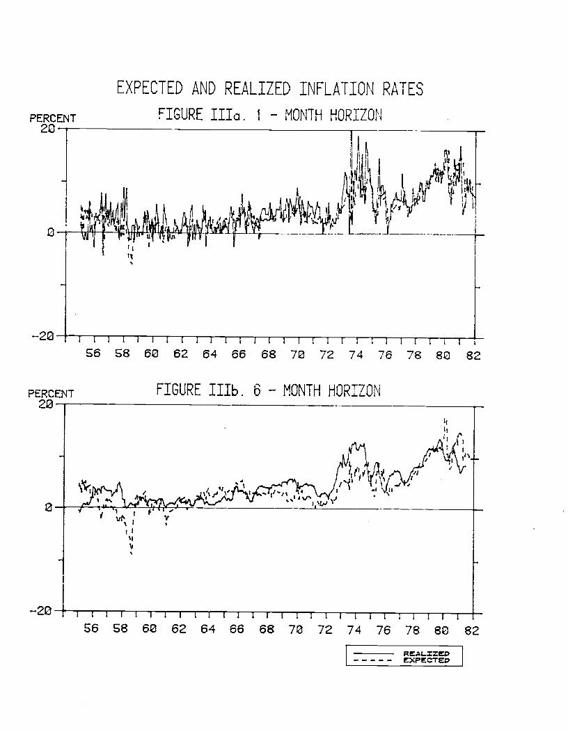
The first proxy for the expected real rate is an out—of—

sample forecast derived by projecting the log of prices at each

point in time on a constant and three lags of data using a con-.

stant coefficient Kalman filter technique. This procedure is

equivalent to reestimating an OLS regression each period.1!i The

resulting monthly expected inflation, at time t, = E(CPIt+iJ

Mlt_8,CPIt_8,IPt_8,BILLS1t5,s0,1,2) — CPI. is presented in

Figure III. By subtracting the expected inflation from BILLS1,

the one—month nominal interest rate, we generate an ex ante one—

month real rate, r, which is presented in Figure IV.

Movements of the one—month ex ante real rate which we

have constructed are to a large extent dominated by the movements

in expected inflation, which are subtracted from the more stable

nominal rate. One possible concern with this measure is that if

real rates with longer turity are more important for economic

decisions than short rates, and if inflation expectations over

-20

EXPECTED AND REALIZED INFLATION RATES

FIGURE lIla. 1 — MONTH HORIZON

FIGURE IIIb. 6 — MONTH HORIZON

PERCENT20

PERCENT20

56 58 60 62 64 66 68 72 72 74 76 78 80 82

56 58 62 62 64 66 68 72 72 74 76 78 80 82[[ EXPECTED

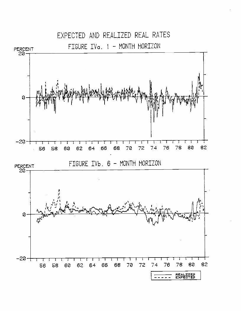
EXPECTED AND REALIZED REAL RATES

FIGURE IVa. I — MONTH HORIZON

FIGURE IVb. 6 — MONTH HORIZON

PERCENT20

PERCENT22

6 S8 6 62 64 66 68 70 72 74 76 78 80 82

6 58 60 62 64 66 68 70 72 74 76 78 80 82

—9—

longer horizons are less volatile, then a measure of the real rate

over a longer maturity might explain more of the variation in

output than one with a shorter maturity.

In order to test this hypothesis and to see whether the

results we found were sensitive to our measure of the real rate,

we have experimented with several other measures including a

quarterly real rate, a six—month real rate, and a one—month ex

post real rate..V Although the longer naturity real rates are

much smoother than the short rates, the qualitative properties of

the response functions and decompositions of variance were not

affected by the different definitions. In fact, we found that

innovations in the one—month real rate, despite the fact that they

are approximately 50 percent larger than innovations in the six—

month rate, actually explained more of the forecast variance of

output.

Our monthly ex ante real rate series were employed in

several four variable, autoregressive systems using six lags and a

constant term in each equation. The major difficulty in inter-

preting these systems arises from the strong contemporaneous

correlation between innovations in expected inflation and innova-

tions in the expected real rate. Table II reports the variance—

covariance matrix of the innovations arising from systems which

include industrial production, money, nominal rates, and expected

inflation or real rates. These matrices are singular, of course.

— 10 —

Table II

Variance—Covariarice Matrices of Innovations(Entries Below Diagonal are Correlations)

One—Month Real Rate

(Monthly data 1955:7 to 1981:12)IF Mi BILLS1 P r

iF .000081 .000003 .000636 —.003660 .004296Ml .11 .000010 .000397 .001705 —.001308BILLS1 .13 .22 .310370 .2602140 .050122

F —.28 .36 .32 2.1582 —1.8980

r .34 —.29 .06 —.93 1.91481

Six—Month Real Rate

(Monthly data 1955:7 to 1981:12)IF Mi BILLS6 F r

IF .000083 .000002 .000655 .0017114 —.001059Mi .08 .000010 .0001431 .001823 —.001392BILLS6 .16 .29 .211320 .1145930 .065387

P .18 .54 .31 1.0759 —.93001

r —.12 _.43 .114 —.90 .995140

One—Quarter Real Rate

(Quarterly data 1956:1 to 1981:4)IF Mi BILLS 3 F r

IF .0003714 .000030 .oo44oi .0062714 —.001873Ml .29 .000030 .000927 .003767 —.002839BILLS3 .30 .22 .591448 .51677 .077712

P .20 .40 2.7542 —2.2374

-.06 -.34 .07 -.89 2.3151

As can be seen in Table II, there is a strongly negative

correlation between innovations in expected inflation and innova-

tions in the real rate (—.93 for the one—month rate). Also strik-

ing is the fact that the variance of both expected inflation

innovations and real rate innovations in these systems is four to

— 11 —

six times larger than that of nominal rate innovations. Appar-

ently, most of the innovations to expected inflation are nega—

tiveJ.y correlated with innovations to real rates so as to leave

the nominal rate largely unaltered. It is interesting to note the

strong positive correlations among expected inflation, Ml, and

nominal rate innovations.-.J The positive correlation between

money and nominal rate innovations suggests that demand shocks

have dominated the unexpected niovemens in money. The strong

positive correlation between nominal rates and expected inflation

implies that a given movement in nominal rates is much more likely

to reflect changes in expected inflation than changes in the real

rate. For example, based on the correlations in Table II, in the

quarterly system a 1 percent innovation in the nominal rate is

most likey to reflect an increase of .86 percent in expeted

inflation and an increase of only .i1 percent in expected real

rates.

The high negative correlation between real rate innova-

tions and expected inflation innovations implies that, unlike the

system examined in Section I, the qualitative properties of the

moving average response graphs and the decomposition of variance

might be expected to depend on the particular orthogonalization

chosen. This is confirmed in Table III, which reports the vari-

ance decomposition of output in three alternative systems which

all lead to equivalent predictions of future values.

— 12 —

Table III

Decomposition of Variance of Industrial Productionat Various Forecast Horizons With Various Orderings

of Ex Ante Inflation and Real Ratesa

Month IF Vfl P r or BILLS1

12 82.1 1.14 9.7 6.7

24 57.1 3.0 27.6 12.2

36 42.2 14.1 141.2 12.6

48 34.8 4.1 149.3 11.8

Month IF Ml BILLS1 P or r

12 82.1 1.14 11.3 5.124 57.1 3.0 24.4 15.14

36 142.2 14.1 28.6 25.1

148 314.8 14.1 29.4 31.7

Month IF Ml r P or BILLS1

12 82.1 1.4 3.9 12.6

24 57.1 3.0 11.6 28.2

36 142.2 14.1 19.8 314.0

148 34.8 4.1 25.5 35.6

a The table is based on one—month to maturity real rates. Data are monthlyfrom 1955:7 to 1981:12

The linearity of the vector autoregression system and

the identity, real rate nominal rate — expected inflation,

implies that given one of these variables, the predictive content

for output is identical whichever of the other two variables is

included. Thus, in the first vector autoregression examined in

Table III, the third column is orthogonalized innovations in

expected inflation and the fourth column can be interpreted alter-

natively as orthogonalized innovations in either nominal rates or

real rates.

— 13 —

As we saw in the earlier systems, a high proportion of

the varaince in industrial production is explained by innovations

in interest rates. In the system shown here, over 60 percent of

the variance of industrial production at a four—year horizon is

explained by orthogonalized innovations in any two of the vari-

ables, nominal rates, real rates, and expected inflation. Using

our other measures of the real rate, this proportion varied from

39.4 percent for the six—month rate to 64.8 percent for the quar-

terly system using a bill rate with three months to maturity.

As can be seen in Table III, the proportion of this

variance explained by orthogonalized innovations in expected

inflation or real rates varies considerably with the ordering

chosen. This sensitivity is to be expected given the high corre-

lation between the two. Nonetheless, it is possible to detect a

pattern which suggests that expected inflation may be the more

important factor. Comparing the first system in Table III with

the third system, it can be seen that of the 6i.i percent of

variance explained, mich more is attributed to expected inflation

innovations when they are third in the ordering than to real rate

innovations when they are third. Shown below is the breakdown of

this variance for each of the four systems we looked at.

— i4 —

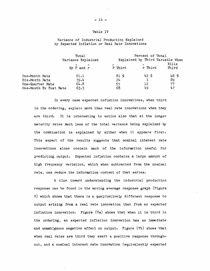
Table IV

Variance of Industrial Production Explainedby Expected Inflation or Real Rate Innovations

Total Percent of Total

Variance Explained Explained by Third Variable WhenBills

By P and r P Third r Third Third

One—Month Rate 61.1 81 % 42 % 48 %Six—Month Pate 39.4 24 1 89One—Quarter Rate 64.8 55 12 77One—Month Ex Post Rate 63.3 68 49 47

In every case expected inflation innovations, when third

in the ordering, explain more than real rate innovations when they

are third. It is interesting to notice also that at the longer

maturity rates much less of the total variance being explained by

the combination is explained by either when it appears first.

This aspect of the results suggests that nominal interest rate

innovations alone contain much of the information useful for

predicting output. Expected inflation contains a large amount of

high frequency variation, which when subtracted from the nominal

rate, can reduce the information content of that series.

A clue toward understanding the industrial production

response can be found in the moving average response graph (Figure

v) which shows that there is a qualitatively different response to

output arising from a real rate innovation than from an expected

inflation innovation. Figure (Va) shows that when it is third in

the ordering, an expected inflation innovation has an immediate

and unambiguous negative effect on output. Figure (Vb) shows that

when real rates are third they exert a positive response through-

out, and a nominal interest rate innovation (equivalently expected

PERCENT2---

RESPONSES OF INDUSTRIAL PRODUCTION — EX—ANTE EXPECTATIONSESTIMATION PERIOD 195: 1—1981 12

MONTHLY DATA. I — MONTH EXPECTATIONS

FIGURE Va. INCLUDING EXPECTED INFLATION

RZPONSS TO INNOVATION INiINDUSTRIAL PRODUCTIONMONEY STOC)- — EX-ANTE REAL. RATE— — — - NOMINAL RATE

— —.-.—-—— — — — —

—— — — — — — — — — — — — — — — — —

L1III1IIIII1lIiII1JLIT1L1iI1L1IIIL!1III1IIL—2

MONTHS12 24 36 48

PERCENT2

FIGURE Vb. INCLUDING EXPECTED REAL INTEREST RATE

RESPON$S TO INt'iCVATZCN IN sINDUSTRIAL PP.CDUCTICNMONEY STCJ<— - — EX—ANT INPLATION— — — - NOMINAL R.&T

12 24 36 48MONTHS

RESPONSES OF INDUSTRIAL PRODUCTION — EX—ANTE EXPECTATIONSESTIMATION PERIOD 19S: 1—1981:12

QUARTERLY DATA, I — QUARTER EXPECTATIONS

FIGURE V10. INCLUDING EXPECTED INFLATION

— — —. — — — ——

4 8 12[RESPONSES TO INNOVATION IN'

INDUSTRIAL PRODUCTIONMONEY STOCK— — — EX.—AMTE INPLATION

— — — - NOMINAL RATE

FIGURE VIb. INCLUDING EXPECTED REAL INTEREST RATE

—'.' — -.-—. — — — — — — — — — — —

— —.—.. . \ '— —

/

RESPONSES ro INNOVATION ININDUSTRIAL PRODUCTION

STOCK— - — EX—ANTE REAL RATE—— — - NOMINAL RATE

PERCENT2.E

I I I LI I I I I I I t i

QUARTERS16

—

PERCENT2.S

0.2

—2.5-

\\\N

N — —. — — — —

I I I I I I I 1

4 128QUARTERS

16

— 15 —

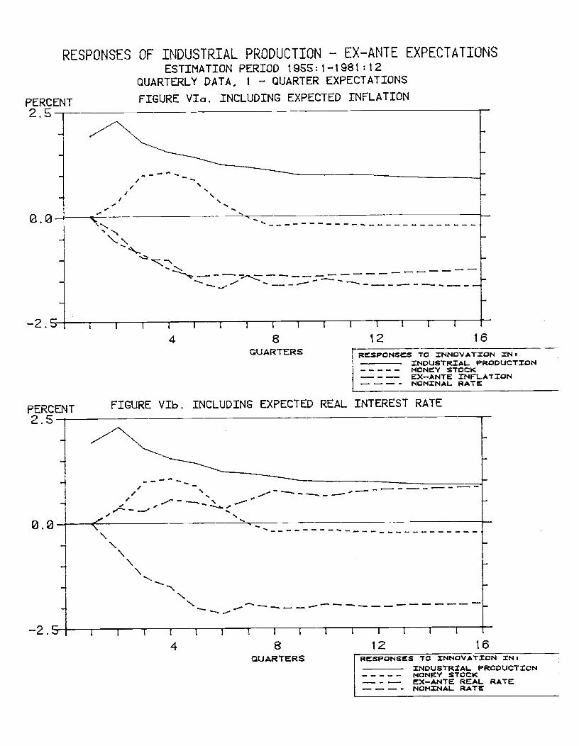
inflation innovation) has a depressing effect past the four—month

horizon. This same pattern ias evident in all the systems which

we looked at. Figure VI shows these responses in the quarterly

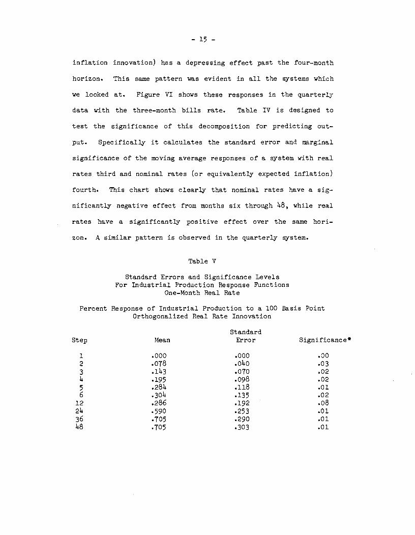
data with the three—month bills rate. Table IV is designed to

test the significance of this decomposition for predicting out-

put. Specifically it calculates the standard error and marginal

significance of the moving average responses of a system with real

rates third and nominal rates (or equivalently expected inflation)

fourth. This chart shows clearly that nominal rates have a sig-

nificantly negative effect from months six through 248, while real

rates have a significantly positive effect over the same hori-

zon. A similar pattern is observed in the quarterly system.

Table V

Standard Errors and Significance LevelsFor Industrial Production Response Functions

One—Month Real Rate

Percent Response of Industrial Production to a 100 Basis PointOrthogonalized Real Rate Innovation

Standard

Step Mean Error Significance*

1 .000 .000 .00

2 .078 .0140 .03

3 .1143 .070 .0224 .195 .098 .02

5 .2814 .118 .01

6 .3014 .135 .0212 .286 .192 .08

214 .590 .253 .01

36 .705 .290 .01

148 .705 .303 .01

— i6 —

Percent Response of Industrial Production to a100 Basis Point Orthogonalized Nominal Rate

(or Expected Inflation) Innovation

Standard

Step Mean Error Significance*

1 .000 .000 .00

2 .216 .09L .01

3 .248 .169 .06

.053 .232 .43

5 —.217 .286 .22

6 —.527 .335 .06

12 —i.9 .370 .00

2 —i.6i .186 .0036 —1,655 .622 .00148 —1.1495 .735 .01

One Quarter Real Rate

Percent of Response of Industrial Production to a100 Basis Point Orthogonalized Real Rate Innovation

Standard

Step Mean Error Significance*

1 .000 .000 .00

2 .267 .1145 .03

3 .219 .228 .1614 .1413 .280 .06

6 .255 .360 .238 .5140 .1440 .09

10 .14)47 .1498 .1712 .568 .559 .1)4

14 .580 .613 .15

16 .609 .663 .17

— 17 —

Percent Response of Industrial Production to a100 Basis Point Orthogonalized Nominal Rate

(or Expected Inflation) Innovation

StandardStep Mean Error Significance*

1 .000 .000 .002 —.847 .276 .003 —1.746 .468 .004 —2.079 .586 .006 —2.994 .707 .008 —2.806 .787 .0010 —2.738 .867 .0012 —2.815 .982 .0014 —2.738 1.139 .0116 —2.677 1.324 .01

*Sjgnjficance is used here in a Bayesian sense to refer to theintegral, given a noninforinative prior, of the posterior distribu-tion of the response function less than zero, or greater thanzero, whichever is less.

Up to this point we have considered responses of indus-

trial production in systems which include an inflation expecta-

tions or real rate variable generated out—of—sample, but which do

not include actual inflation rates. In these systems, we have

displayed the response to the orthogonalized innovations in the

included variables. Another approach we consider is to estimate

an unrestricted vector autoregression on the original observed

variables, industrial production, money inflation and interest

rates, and then to measure the expected inflation and implied real

rate implicit in the system. It is then possible to construct

responses of industrial production to orthogonalized innovations

in expected inflation or real rates even though these variables

are not entered directly as observable in the system.

We follow the same technique applied earlier of generat-

ing, in turn, responses to expected inflation and real rate info—

— i8 —

vations when they are third in the orthogonalization ordering.

These shocks are defined as linear combinations of the observable

innovations where the weights are obtained from the coefficients

in the inflation equation. The qualitative properties of these

responses, shown in Figure VII, are similar to those generated

directly from out—of—sample expectations.IJ Again, when we decom-

pose the nominal rate symmetricalJ.y into expected inflation and

expected real rates, the data suggest that it is the expected

inflation component which leads to the negative response of indus-

trial production.

Another interesting observation in these systems is that

the real rates we looked at are largely exogenous. The real rate

responds mostly to itself, dampening very quickly. At the 48—

month horizon, 68 percent of its own variance is explained by its

own innovations for the one—month out—of—sample ex ante rate and

90 percent for the one—month ex post case. The percent of vari-

ance explained by own Innovations is 56 percent for the one—

quarter rate and 62 percent for the six—month rate. Response

functions of the real rate are shown in Figure IX.

III. ecific Tests With Vector Autoregressions

The preceding descriptive empirical findings cast doubt

on the money—interest—output link suggested by Keynesian and most

demand—driven models of output. Not only did the real rate fail

to reflect any systematic influence from money or prices, but

output appeared to respond to expected inflation more than to the

real rate. In this section, we will examine these results more

carefully, testing specific restrictions on the reduced form which

reflect on the validity of various economic theories.

RESPONSES OF INDUSTRIAL PRODUCTIONIN SAMPLE EX—ANITE EXPECTATIONSMONTHLY DATA.. 1949:2—1981 :8

FIGURE VIle. INCLUDING EXPECTED INFLATIONPERCENT2

0

—2

PERCENT

12 24MONTHS

36 48

FIGURE VIIb. INCLUDING EXPECTED REAL INTEREST RATE

RSPCNSS T0 ZNNCVATIN ININDUSTRIAL PRODUCTION

STOCK— - — EX—ANTE INFLATION— — — - NOMINAL RATE

e

—2

T12 24

MONTHS

III I I I I III I I I I I I I I I I I I III II I I I I Ii III I I I

RSPONSS TO INNOVATION IN iINDUSTRIAL PRODUCTION

STOCK— - — EX—ANTE REAL RATE—— — - NOMINAL RATE

36 48

RESPONSES OF INDUSTRIAL PRODUCTIONIN SAMPLE EX—ANTE EXPECTATIONSQUARTERLY DATA.. 1950:2-1981:2

PERCENT FIGURE VIlla. INCLUDING EXPECTED INFLATION

2.5

——2.5—— r4 8 12 16

QUARTERS ict it'zINDUSTRIAL. PRODUCTICN

STCCKI

— - — EX—ANTE INFLATIONL — — — - NOMINAL

PERCENTFIG VIIIb.INCLUDING EXPECTED REAL INTEREST RATE2.5 -

N

-

•— _— — — —.r —. — —

N ——--/

i r i i r i i i

4 8 12 16QUARTERS rspoNss -ro INNOVATION IN:

INDUSTRIAL PRODUCTIONSTOCJ(— - — E'<—ANTE REAL RATE— — — - NOMINAL RATE

RESPONSES OF THE EX—ANTE REAL INTEREST RATE

BASIS PTS. FIGURE IXa. 1 MONTH RATE2-

\

—— - _____J \'.-;.: _.- ____________________________________________________

MONThS

BASIS PTS.2-

\

FIGURE IXb. 1 — QUARTER RATE

=-____ — - —

QUARTERSRESPONSES TO INNOVATION INt

INDUSTRIAL PRODUCTIONMONEY STOCK— - — EX—ANTE REAL RATE— — — - NOMINAL RATE

1—

0

—1

:—.--—

ill Ill ill I lilt 11111 III till liii 11111111 ill I liii12 24 36 48

—1

-.-.. ,/ —V—--—---—--

— -V

I I I I I I I I I I I I I I4 8 12 16

— 19 —

A. IS THE REAL RATE EXOGENOUS?

We begin by testing a restriction, suggested by our

Section II results, which we feel is incompatible with theories

that emphasize a role for the real rate of interest in transmit-

ting monetary disturbances to the real economy. In particular, we

test the restriction that past money, prices, and income have no

additional predictive content for current real rates, given past

real rates. That is, we test the hypothesis that the real rate is

exogenous, or Granger causally prior, in the content of this four

variable system.

Because the ex ante real rate is unobservable, testing

this hypothesis requires an auxiliary hypothesis of how agents

forecast future prices. We will assume that agents' expectations

are rational, which in the context of our information set and in

the absence of any further restrictions, identifies price expecta-

tions with the projection of future prices on current and lagged

endogenous variables.

As is often the case, the imposition of the rational

expectations hypothesis here leads to complicated, nonlinear

cross—equation restrictions. While the imposition of these re-

strictions is costly in terms of computations, we find that it

generates test statistics which have greater power to differen-

tiate among hypotheses than other approaches such as Faina (1975),

Fania (1982), Nelson and Schwert (1977) and Garbade and Wachtel

(1978).

Interpretation of causal orderings as indicative of

behavioral or structural relationships is a complicated and subtle

— 20 —

issue (see Sims (1972, 1975)). Nevertheless, we would expect that

IS—LM models would, in general, reject exogeneity of the real

rate. Thus, we believe the failure to reject would raise ques-

tions about the validity of such models. We believe the test also

bears on the empirical validity of the informationally constrained

equilibrium models, even though our measure of the expected real

rate ignores the limitations on current period information which

are essential ingredients of these models. While in both cases we

can imagine versions of the model which would fool us into accep-

tance of the hypothesis that the real rate is exogenous, we find

these special cases implausible.

The compatibility of this hypothesis with the IS—LM

model, the Lucas—Barro model, and the Grossman—Weiss model will

each be considered in turn.

The IS—LM Model

A central feature of Keynesian IS—LM analysis is the

idea that changes in the demand or supply of nominal balances can

change the real interest rate. Keynesian theory achieves this

connection by invoking sluggish nominal price adjustments in

nonfinancial markets, particuarly the labor market.

Consider the following IS—LM model

IS y = _1r + > °

M Ci)LM =

a1Y— a2(rt+I[) + • > 0, a2 > 0

where rt is the real rate and ll is expected inflation, c repre-

sents all exogenous spending (including government spending and

— 21 —

variations in desired investment not related to interest rate

movements), 4 represents random influences on real nzney demand

(the state of "liquidity preference"). The reduced form equations

for the endogenous variables, rt, are given by

r = + Y2(mt_t) +311t

(2)=

T14t+ 15(mt_t) + 611t

where

— zl — —1 — —l1—

21Bl 2 — 2181—

(3)

_______ 81 812 Mt= 21l 5 a2181 and=

a2+8181m =

An implication of this theory is that, unless 8, the

interest elasticity of investment demand were infinite, monetary

policy can affect output only to the extent it affects the ex ante

real rate.

Under what auxiliary hypothesis can this model be com-

patible with the finding that

E(rt+iJrt_5,s>O) = E(rt+iIrt_5,M.,Pt5,Yt,s>O) ? (4)

One possibility is that, over the observed sample, it

was the deliberate objective of Fed policy to set expected real

rates in such a way that the tio hypothesis are observationally

equivalent. This iight arise, for example, if the policy objec-

tive were to minimize the variance of output, E(Y_y) , by set-

ting r (y—c). If followed a univariate autoregressive

— 22 —

process, then so would rt. Although we cannot reject this possi-

bility a priori, it is unlikely that desired interest rate targets

could be expressed in terms of any single factor, let alone the

past history of interest rates. It certainly appears as if policy

has aimed for both price and output stability. Since prices and

output exhibit some independent variation, it is implausible to

take the finding that the real rate is exogenous as indicative of

a particular policy reaction function.

Another possibility which could explain the lack of any

influence from past money, prices, and output on current ex ante

real rates is that the IS curve is horizontal. This would be true

1' the interest sensitivity of demand, were infinite, so that

variations in money supply or demand affected only output without

a measurable impact on interest rates. This possibility is both

highly implausible in a monthly system and is easily rejected by

subsequent findings.

Still a third possibility, less easily dismissable, isthat over the sample period most variations in money supply, nit,

were passive responses to money demand shocks. Under this

hypothesis, there would be no added explanatory power from past

money to future real rates. This hypothesis requires either no

deliberate attempt on behalf of the Fed for controlling real

rates, except insofar as interest rate targets depend only on

lagged values, or that policy—induced interest rate variations

have been sufficiently small compared with exogenous money demand

shifts so that our procedure cannot distinguish this variation

from variation due to sample errors.

— 23 —

A fourth possibility which could give rise to a spurious

finding of exogeneity concerns the role of omitted variables.

Suppose the true reduced form for ex ante real rates is given by

vm+ w z.+c=0 • =0

where is a vector stochastic process of omitted variables and

is a vector conformable to Zt. Suppose

EEztKImt,rntl...] = aJ (6)

Then, in populations, the regression coefficients of rt on lagged

m's are given by

h v1+ wKaK j=0... (7)K=0

While it is certainly possible that hj's will be zero,

even though the vj's are nonzero, this is highly unlikely as it

requires an extreme coincidence between the v's, w's, and a's.

These possibilities, while being neither mutually ex-

clusive nor exhaustive seem sufficiently implausible to us that

failure to reject the hypothesis that the real rate is exogenous

casts strong doubt on the Keynesian notion that monetary policy

has affected output through changes in the real rate of interest.

The Lucas—Barro del

The model presented in Lucas (1972) and modified by

Barro (1976, 1980) emphasizes the effects of unperceived monetary

injections on labor supply by altering perceptions of real rates

of return. By positing barriers on current period information

flows, these models draw a sharp distinction between expectations

— 2 -

based on complete current period information and the expectations

held by a representative trader. Nevertheless, the hypothesis

that the real rate (based on complete current information) is

exogenous would seem incompatible wiht most intertemporal versions

of these models.

The original versions of these models assumed all random

disturbances to be serially uncorrelated, and all information lags

to be at most a single period. These features, while inessential,

imply that both concepts of the real rate would be serially inde-

pendent. Thus, in this limited sense, the models are compatible

with the finding that the real rate is exogenous. However, if

these models are appended to be consistent with the fact that

there are substantial serial correlations in most macroeconomic

time series, then it is difficult to reconcile the models.

To see this, imagine that the ex ante real rate, con-

ditioned on aggregate information, is given by

n n_I

r A1÷ 1_ + • m, + (8)

=1 ' =0

where = — E[nltlinformation as of t—l] is the unexpected

component of money and is a stochastic vector of real factors

which affect real rates (e.g., productivity, thrift, government

expenditures). Exogeneity of the real rate in the context of a

system which includes a measure of real production requires either

that the measure is uncorrelated with components of t or that the

are all zero. Theories which place an emphasis on a confusion

between unperceived monetary injections and persistent real fac-

tors affecting the ex ante real rate would generally predict a

— 25 —

systematic response of the real rate to changes in real produc-

tion. A failure to reject exogeneity of the real rate thus raises

questions about the empirical importance of this channel for

monetary disturbances to have real effects.

The Grossman—Weiss Model

This model also assumes incomplete information so that

the expected real rate based on complete current period informa-

tion differs from the expectations held by a representative

trader. The model determines the ex ante real rate based on

complete current period information to be equal to rt = (1—a)

E[Ct+i_Ctlavailable information at tJ where a is a parameter of

preferences and = (log) per capita consumption.

As in the Lucas—Barro model, the compatibility of this

theory with an exogenous real rate depends crucially on the nature

of the exogenous stochastic disturbances. In the original version

of the model, it was assumed that both monetary and real distur-

bances were serially independent, which resulted in serially

independent consumption. In this case, the ex ante real rate is a

first order moving average process and the real rate is exoge-

nous. However, if the model is modified to be consistent with

serially correlated consumption, then the real rate will not

appear to be exogenous. As in the models which emphasize unper-

ceived money, when there are both real and monetary factors which

determine the real rate, and these factors have lagged effects, we

would not expect the real rate to be exogenous.

The three theories we have examined have in common that

the real rate of interest plays a crucial role in the generation

— 26 —

of business cycles, and that (except under special circumstances)

its behavior is a function of lagged real and monetary distur-

bances. Any model with these two characteristics would appear to

be challenged by the finding that in a system with real and mone-

tary variables, the real rate of interest is exogenous.

B. WHAT CAUSES OUTPUT?

A central issue of most business cycle theories is the

transmission mechanism between changes in the supply or demand for

money and the level of economic activity. The importance of money

for predicting output was demonstrated by Sims in 1972 in a 'oi—

variate system and was generally accepted as evidence of real

effects of purely monetary phenomena. Explaining this relation-

ship has occupied a central role of recent theoretical develop-

ments. Modern theories share with Keynesian theory the idea that

monetary phenomena affects real variables by altering perceptions

of ex ante real rates. In light of the results in Section II in

which real rates appear significantly less useful for predicting

output than nominal interest rates and real rates themselves

appear to be exogenous, we are led to question the usefulness of

both Keynesian and equilibrium theories for explaining the ob-

served correlations between nominal and real variables.

We first confirm Sim's finding that industrial produc-

tion is not exogenous in a four variable vector autoregression

with nominal rates, money, and prices. We then go on to test

whether the observed effects from nominal quantities can be ex-

plained through lags of the real rate alone. Given our Section II

results, we would expect this hypothesis to be rejected.

— 27 —

Our next set of hypotheses are not implications of any

completely articulated theory, but are designed to examine the

descriptive results presented in the previous section. In par-

ticular, we wish to investigate the channels, if any, through

which monetary disturbances affect output.

We first test whether all lagged financial effects can

be filtered through lagged levels of nominal interest rates. Even

if this is true, however, it does not eliminate an indirect role

for money. If lagged money helps to predict nominal interest

rates, then it helps in predicting future output as well. In

order to examine this issue, we test whether output and nominal

rates are block exogenous.

Given the identity between nominal rates, real rates and

expected inflation, we also find it interesting to test the hy-

pothesis that all financial effects on output are filtered through

lags of expected inflation. By comparing the results of tests of

the above hypotheses, we can measure the relative explanatory

power for output of each of the components of nominal rates.

Finally, we test directly whether the decomposition of nominal

rates significantly helps explain output.

In examining the importance of monetary disturbances, we

are led to another set of possible restrictions on the system

which would eliminate a role for nney in predicting output.

these hypotheses are that lags of nominal rate or expected infla-

tion innovations are sufficient to capture all lagged financial

effects. Since innovations are, by construction, orthogonal to

all past variables, these are tests of block exogeneity of output

— 28 —

and nominal interest rate or expected inflation innovations in the

context of the four variable autoregressive systems.

C. EMPIRICAL RESULTS

Our tests will be based on the standard likelihood ratio

statistic, and in interpreting our results we will present mar-

ginal significance levels based on asymptotic distributions giving

the probability, under the null hypothesis, of observing test

statistics of the given mgnitude. We do riot, however, interpret

these significance levels literally. Two problems, in particular,

bias the significance levels. First, given the large number of

restrictions we are testing, there is ample reason to question the

validity of the asymptotic distribution approximation for samples

of the size we have. Direct calculation of those distributions,

while possible through numerical simulations, would be prohibi-

tively expensive. Second, our test procedures are being applied

to the same data set which suggested the hypotheses to us in the

first place. Because of these problems, we put little weight on

the absolute levels of the test statistics. Rather, we wish to

compare the relative fit of different restrictions. We find the

classical hypothesis testing framework, with a fixed unrestricted

vector autoregression as the alternative, a useful device through

which we can investigate specific questions by looking at the

degree to which various hypotheses are consistent with the data.

In this context, we interpret the calculation of a significance

level of a likelihood ratio statistic as a natural way to correct

the relative fits of different restrictions for differences in

degrees of freedom.

— 29 —

The hypothesis that the ex ante real rate of interest,

rt, is a function of only its own lagged values, a constant term,

and an uncorrelated random error, can be written as follows:

r = b rtj +r+ Ut.

The assumption of rational expectations implies

rt— t11t+ (io)

where Rt is the observed nominal interest rate and t11ti is the

projection of the annualized growth rate of the price level from t

to t+1 on information available at time t.

Substitution of (10) into (9) leads to the following

expression for the nominal interest rate:

= + — + cr +Ut (II)

This equation imposes testable restrictions across the

autoregressive representation for Rt, 11t' and the other variables,

Z., in the information set individuals use in projecting future

values of 1.

Suppose a finite order autoregressive representation

exists for the K—vector

x. = [R 11t Z].

L

X= AXt&+C+11t (12)

£ =1

The 1th equation of this representation has the scalar

form

— 30 —

X aiXL+Ci+r1 (13)

j=1 L=1

where is the coefficient on the &th lag of the jth component

of X. Thus, for example, the projection of inflation during

period t on observables at time t—l, is given by

= + +

£=l+ C2 (i14)

The restrictions on a vector autoregression implied by-

(9) are generated by using (114) to replace all expected inflation

terms in (ii) with projections on observables, collecting terms

with Rt on the left—hand side, and then projecting both sides on

information available at time t—1. The resulting equation is a

projection of Rt on information available at time t-l which

equates each of the coefficients in the Rt equation, 4, with a

function of the b,'s, and the a's for i = 2, ... K. For ex-

ample, for & in,

a' = (121)(15)

Because there are L lags in each of the projections of

the observed variables, lags of the real rate become functions of

observations more than L periods earlier than the current pe-

riod. Thus, the reduced form projection for R tmist include rn—i

more lags than each of the other equations. This requires us to

impose (9) as a restriction on a vector autoregressive system with

L+m—l lags on all variables in the R projection and L lags of all

variables in the other projections.

— 31 —

Equations similar to (15) express each of the coeff i—

cients in the R projection as a function of the other coeffi-

cients. Given the introduction of the rrrfl new free parameters, b1

and cr, these equations impose K*(L+m_1)_m nonlinear re-

strictions on the parameters of the vector autoregression.

In tests concerned with what causes movements in output,

we consider four types of explanatory variables, observable quan-

tities, unobservable quantities, and innovations in each. Tests

with observable quantities are easiest to implement. The likeli-

hood ratio of one equation with linear restrictions relative to

the corresponding equation in an unrestricted vector autoregres-

sion is equivalent to the likelihood ratio test of the entire

system with and without the equation so restricted. This result

is shown by Doan (1980) using results in Revankar (1971). These

results do not apply, however, when the alternative system has

different numbers of lags in different equations.

Tests using unobservable quantities, expected inflation

or real rates, are implemented in a manner similar to that de-

scribed above for testing exogeneity of the real rate. Substitu-

tion of projections on observables for these quantities leads to

nonlinear restrictions across equations.

The tests which utilize lagged innovations as explana—

tory variables follow essentially the same estimation procedure as

for those with unobservable quantities. Innovations in nominal

interest rates, for example, are defined by

Rt = Rt_ E[RtIYt 5,Rt ,Mt s(16)

— 32 —

The expectation is determined by the autoregressive representation

for R, and the R's can be substituted out in a manner similar to

that in the earlier tests.

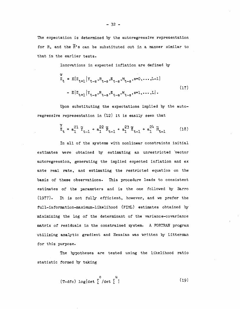
Innovations in expected inflation are defined by

= E[fit+iIYt ,Rt fit ,Mt,s=O,... ,L—lJ

(17)— EEfit+iIYt,Rt,llt,Mt,S=1,...,Ll.

Upon substituting the expectations implied by the auto—

regressive representation in (12) it is easily seen that

= a Y1 + a2 + a3 + a (18)

In all of the systems with nonlinear constraints initial

estimates were obtained by estimating an unrestricted vector

autoregression, generating the implied expected inflation and ex

ante real rate, and estimating the restricted equation on the

basis of these observations. This procedure leads to consistent

estimates of the parameters and is the one followed by Barro

(1977). It is not fully efficient, however, and we prefer the

fuj.l—inforniation—maximum—likelihood (F1ML) estimates obtained by

minimizing the log of the determinant of the variance—covariance

matrix of' residuals in the constrained system. A FORTRAN program

utilizing analytic gradient and Hessian was written by Litterman

for this purpose.

The hypotheses are tested using the likelihood ratio

statistic formed by taking

(T—dfc) logidet /det ] (19)

— 33 —

where T is the number of observations in each equation, dfc is a

degrees of freedom correction suggested by Sims (1980b) equal to

the number of parameters in each equation of the unrestrictedC

system, is the covariance matrix of residuals in the con—U

strained system, and is the covariance matrix of residuals in

the unrestricted system.

In implementing our tests we found it difficult on a

priori grounds to choose a particular interest rate to focus on.

Theories generally do not differentiate between rates at different

maturities, but certain trade—offs clearly exist. Longer maturi-

ties are probably more relevant signals for investment decisions

and in the case of real rates will be more robust to timing errors

in the measurement of prices. Short rates, however, are likely to

be more responsive to monetary disturbances and less subject to

time aggregation problems. It will also be easier to forecast

inflation rates over shorter time horizons, although those fore-

casts will include more short—run variation than forecasts over

longer horizons. Our reaction here is similar to our response in

Section II; we present all of the results for two different inter-

est rate maturities.

The first set of data is monthly observations from 18:i

to 81:8 on Ml, end of month rates on Treasury bills with one month

to maturity, industrial production and the consumer price index

less shelter. The second set is quarterly observations from 8:i

to 81:2 on Ml, end of quarter rates on Treasury bills with three

months to maturity, industrial production and the consumer price

index less shelter. In the quarterly system values of money,

— 314 —

output and prices are taken to be the values of those variables

for the third nnth of the given quarter. All data were logged

prior to estimation, and prices were converted to annualized

inflation rates by differencing the logs and rriiltiplying by the

appropriate factor.

— 35 —

Table VI

}typothesis Test Results

Monthly Data

Null Log Degress of Marginal

Hypothesis Alternative Determinant Freedom Significance

1. r exogenous A —19.75017 29 .2302

2. Y exogenous B —19.72565 18 .0211.2

3. Y explained by B B —19.75859 12 .0793

4. Y explained 'by M B —19.76887 12 .2115

5. Y explained by It B —19.74509 12 .oi8

6. Y exogenous C —19.72844 42 .1539

7. Y explained by R C —19.76069 36 .3166

8. Y explained by M C —19.77042 36 .4717

9. Y explained by It C —19.74560 36 .1441

10. Y explained by r C —19.74557 36 .1437

11. Y explained by II C —19.75427 36 .2319

12. Y explained by r, It C —19.77773 30 .31111.

13. Y explained by R C —19.76016 36 .3089

i4. Y explained by It C —19.74852 36 .1703

15. Y, R block exogenous C —19.66756 48 .0102

Alternative Vector AutoregressionsEffec—t ive

Log Correc— Number

Lags in Equation Deternil— tion of Obser—

Alternative B Y M It nant Period Factor vations

A 8 6 6 6 —19.84274 48:10—81:8 25 370

B 6 6 6 6 —19.81074 48:8—81:8 25 372

C 6 12 6 6 —19.86860 49:2—81:8 25 366

36 -

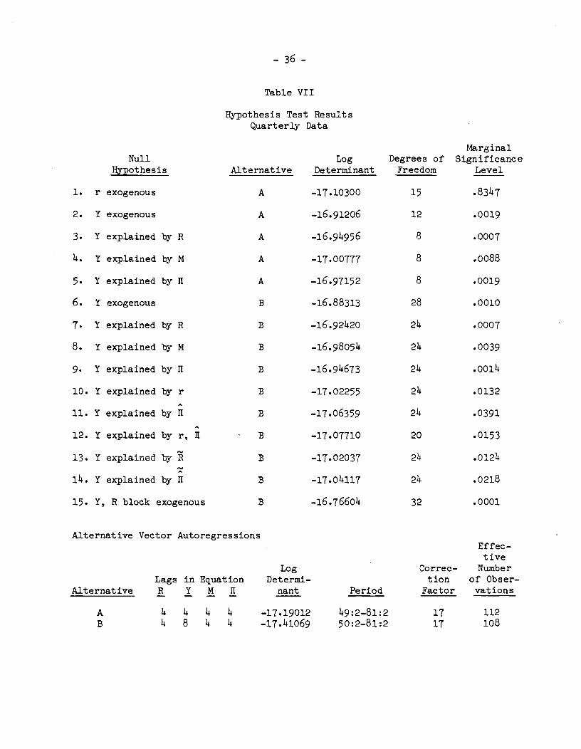
Table VII

Hypothesis Test ResultsQuarterly Data

Lags in EquationB Y M II

4414448144

LogDet errni—

riant

—17. 19012

—17 .141069

Correc-tion

Factor

1717

Effec—t ive

Numberof Obser—vat ions

112108

Null

Hypothesis AlternativeLog

DeterminantDegrees ofFreedom

MarginalSignificance

Level

1. r exogenous A —17.10300 15 .83147

2. Y exogenous A —16.91206 12 .0019

3. Y explained by R A —16.914956 8 .0007

4. Y explained by M A —17.00777 8 .0088

5. Y explained by II A —16.97152 8 .0019

6. Y exogenous B —16.88313 28 .0010

7. Y explained by B B —16.921420 24 .0007

8. Y explained by M B —16.98054 24 .0039

9. Y explained by II B —16.94673 214 .0014

10. Y explained by r B —17.02255 24 .0132

11. Y explained by II B —17.06359 24 .0391

12. Y explained by r, 11 B —17.07710 20 .0153

13. 1 explained by R B —17.02037 214 .0124

14. Y explained by II B —17.04117 24 .0218

15. Y, B block exogenous B —16.76604 32 .0001

Alternative Vector Autoregressiors

Alternative

AB

Period

49:2—81:250:2—81:2

Table VIII

Selected Coefficient EstimatesIn Restricted Equations

(Standard Errors in Parentheses)

Hypothesis 1: Real Rates ExogenousMonthly Data

rt = .965 rt .(.049)

—

Quarterly Datart = .702 rtl + .090 + ut

(.065) (.io6)

Hypothesis 10: Output Explained by Real Rates

Monthly Data= 1.444

(.037)— .00014 rt_l

(.00035)— .0021 rt 5

(.00050)—

— .391 t—2 — .023 t—3 — .116 t—4 — .037 Y—5 +(.067) (.073) (.079) (.080)+ .00042 rt2 — .00122 rt3 + .00116 rt_4

(.00040) (.00042) (.00047)+ .00022 rt_6 + .00757 +

(.00037) (.00436)

.077 t—6(.042)

— .635 t—2 + .008 t—3 + .049 t—4(.384) (.359) (.159)

— .0333 rt_2 + .0283 rt3 — .0072 rt4(.0106) (.0092) (.0047)

Monthly Data= 1.435 Yt_ .410 t—2 + .046 t—3 — .096 t—4 — .063

(.037) (.oio) (.078) (.083) (.081)

+ .00056 — .00087 11t—2 - .00095 11t—3 - .00109 11t—4

(.00036) (.00044) (.00049) (.00056)

(.00057) (.00039) (.00690)

Quarterly Data= 1.677 Yt— — .904 t—2 + .220 t—3 + .027 t4 — .0185 11t_i

(.139) (.292) (.297) (.140) (.0041)

+ .0316 1t2 — .0283 11t—3 + .0041 11t—4 + .4921 + Ut

(.0076) (.0073) (.0040) (.0402)

— 37 —

— .431rt 2 + .235 rt 3 + .077 +

(.071)—

(.045) (.068)

Quarterly Data= 1.577 Y_(.189)

+ .0270 rt_l(.0085)

+ .0086 +(.0406)

Hypothesis 11: Output Explained by Expected Inflation

— .00002 11t—5 — .00016 11t—6 — .00606 +

+ .090 t—6(.043)

— 38 —

We find that the hypothesis that the real rate is exoge-

nous cannot be rejected in either the monthly or quarterly sys-

tem. This finding accords with our interpretation of the Section

II results. In both systems, the real rate appears as an exoge-

nous Markov process (see Table viii).

It is revealing to compare the response of the real rate

to innovations in each of the four variables in both the unre-

stricted system and the first restricted system (Figures X and

XI). These graphs show that no qualitative distortions are intro-

duced by the restriction that the real rate is exogenous. The

unrestricted system permits arbitrary patterns of feedback from

the variables to the real interest rate. The restriction of

exogeneity requires that the effects of these variables can be

filtered through their contemporaneous correlations with the real

rate alone.

The strongest contemporaneous correlations with real

rate innovations are the positive associations with nominal rate

innovations, and negative association with inflation innovations.

Notice that since both inflation and the real rate have

persistent components, the strong negative contemporaneous corre-

lation between real rates and innovations in inflation is enough

to explain the negative correlation between inflation levels and

future real rates observed by Summers (1980) and Mishkin (1980).

Our interpretation of this phenomenon differs, however, from that

of Summers who argues that money illusion is "the most plausible

explanation for the nonresponse of interest rates to inflation."

Since the result is compatible with an economic structure in which

RESPONSES OF THE REAL INTEREST RATE

percent FIGURE xa.Unrestriced

0

—1

Vector Au4oregress ion

12 24 36 48

perent, FIGURE Xb. Restricted Vect.or Auf.oregress I on

.

0—

. /I— .--.

—

- --——

-,

II

—1 III liii lilt III! I III lilt III12 24

I I I I liii I I36

III48

TO XNNOVATZON8 INsI—MONTH TREASURY SILLSINLATXON— - — INDUSTRIAL PRODUCTION———- MONEY

RESPONSES OF THE REAL INTEREST RATE

I I I I I I4 8 12

percent FIGURE XIb. Restricted Vector Autoregression

0

—1

.-F

I I I I I

4 8 12I I I

TO INNOVATIONS INS3—MONTH TREASURY BILLS

— - — INDUSTRIAL PRODUCTIONMONEY

percent FIGURE xia.UnrestricLed Vector Autoregression

e

—1

/p

N / ,"•••.--•

'•-'•-'h.,/.

.

•

I I I I I I16

16

— 39 —

there is no feedback from prices and money to real interest rates,

we conclude that short—run changes in both real rates and infla-

tion can be attributed to the same, as yet unidentified, random

factor.

The results of our hypothesis tests investigating the

transmission mechanism between money and output raise a number of

puzzling questions. Overall, the results are less clear—cut,

leaving room for differing interpretations. For example, the

results from the monthly system differ from those of the quarterly

system. In our discussion, we attempt to focus on those results

which are least equivocal and to point out where uncertainty

remain s.

We first confirm that output is not exogenous in the

context of these four variable au€oregressions. While the rejec-

tion of output exogeneity is unambiguous in the quarterly system,

it is sensitive to lag length in the monthly system. In the

monthly system with six lags, we can reject output exogeneity at

the conventional 5 percent significance level. However, our other

hypothesis are not restrictions of these vector autoregressions.

Our restrictions involve projections on unobservables which are

themselves projections on lagged observables. Thus, for example,

when six lags of the unobservable real rate are included, the

reduced form will contain 11 lags of the observables. Our most

general alternative for each hypothesis in the context of the

monthly system contains 12 lags in the output equation and six

lags in the other equations, and the quaterly system contains

eight lags in the output equation and four lags in the other equa—

— 140 —

tions. All hypotheses involve restrictions on these two sys—

tems. In the monthly system, none of our hypotheses, including

output exogeneity, can be rejected relative to this alternative.

Nevertheless, the significance level can be interpreted as a way

of ranking these alternative hypotheses.

The hypothesis that the effects from nominal quantities

to output can be filtered through lags of the real rate does not

appear to fit the data well. By comparison, lagged values of

expected inflation have far more explanatory power for output than

does the real rate in both the monthly and quarterly system.

However, somewhat puzzling is the finding that nominal rates and

money do better than either of these variables for predicting

output in the monthly system, but noticeably worse in the quar-

terly system. This anomalous result is confirmed by. testing the

hypothesis that for the purpose of predicting future output is

useful to decompose the nominal interest into its expected infla-

tion and expected real rate components. Consistent with the above

findings the decomposition helps only in the quarterly system. A

likelihood ratio test of the restriction that coefficients on real

rates and expected inflation are the same in the output equation,

that is that only nominal rates matter, has a marginal signifi-

cance level of .4178 in the monthly system and .0093 in the quar-

terly system.

Although we find that nominal interest rates are suffi-

cient for predicting output in a monthly system, we can reject the

hypothesis that output and nominal rates are block exogenous in a

four—variable system. This arises because money and prices have

— 4l —

predictive content for nominal interest rates. Thus, we cannot

conclude from these tests alone that money has no predictive

content for output past a one—period forecast horizon. The next

hypothesis is designed to assess the importance of money for

predicting output at any forecast horizon. Specifically, we test

whether three lags of nominal interest rate innovations are suffi-

cient to capture all lagged effects. Since nominal interest rate

innovations are, by construction, orthogonal to all past vari-

ables, this is a test of block—exogeneity of output and nominal

interest rate innovations in a four—variable system. In the

monthly system, this restriction fits surprisingly well, and the

predictive content of six lags of the innovation of the nominal

rate is virtually identical to that of six lagged levels. In the

quarterly system, the innovations have more predictive content

than the levels, although not as much as expected inflation

levels.

IV. A Possible Explanation

A central result of this paper is that there is infor-

mation in the level of nominal rates for predicting future output

which is not contained in the history of past output or past and

future expected real rates. We suspect that this statistical link

between expected inflation and output arises because agents in the

economy have some information about the level of future output,

not directly observable to the econometric investigator, which is

first reflected in nominal quantities. To see how this could

arise, consider the following structural model in which output is

independent of the money supply process.

— —

Yt+1 = Yt + Zt + Ut+i

Mt - Pt =M1 ''t —

(20)— + r

rt = A rtl +

The crucial feature is that there is some information in

which is known to agents in the econonr and is useful for

predicting future output, but is not directly observable to the

econometric investigator.

Suppose the model is closed by specifying a money supply

process

0 (21)

and the exogenous disturbances c., Z., U. are serially indepen-

dent. It is straightforward to show the reduced form equations

for expected inflation and nominal rates given by

—M —M (i.—x)=

l+M2 j +1+M2(i—A) r

(22)-M

Pt =(l+2) t +

1+M2(1—A) r

arid the solutions for the innovations of these variables are

-M -M (i-x)=

1+M2t +

1+M2(1—A) t(23)

-M=

(i+)+

l+M2(1—A) t

— 143 —

This model shows most simpy that nominal interest rate innova-

tions or expecte4 inflatLon innovations will be correlated with

HZ" innovations, and thereby will be useful for predicting output

when Z, is not observed directly. This occurs despite the lack of

structural teedbaclc from past, current, or future money and prices

to output.

Of course, this model could not account for the predic-

tive content of money in a bivariate system. However, it would

not be difficult o change the specification of the money supply

process to be consistent with this finding, as well as other

characteristic features of the data. Consider the money supply

process

Mt = + 6(__i) + 2 u + (214)

We would expect 4, to be negative; the monetary authority reacts

to an increase 5 inflationary expectations by contracting. We

would expect 62 to be positive as the money supply responds posi—

tively to an unexpected increase in output. With this specifica-

tion, the reduced form equation for expected Inflation and changes

in money supply are given by

M (1..6 ) M (i—x)=

8M -( 21+M1 Z -+MA)6) r (25)

6 6l2AMt_l

-(z_z1) l+M2(l-A)-61A)

(26)

x ((l)rti+ct) +141

Ut +1_6 t

— 414 —

and for the innovations of these variables

M M (i—x)(i+ )= —

l+Mt —

l+M2(l—x—61x Ct + 1_6i U + 1_6 t

(27)

6M 6M(l—A) 6

Mt = —

l+M2 t l+M2(l—A)—61At +l_6l

U +l_6i

+

This modification shows how monetary innovations could

be positive'y associated with "Z" innovations and thus be useful

for predicting real output in a bivariate system in a way which is

consistent with the block exogeneity of income and either nomi.nal

rate innovations or expected inflation innovations in the context

of a larger system. A "Phillips Curvet' relationship——a positive

correlation between ex post inflation and lagged output growth——

could arise from this system if 62 is positive, meaning the money

growth rate rises with unexpected output shocks.

This model suggests an empirical test of the hypothesis

that the inflation—output link is spurious because inflation is

proving for other information relevant to predicting future out-

put. If this view is correct, we would expect that innovations in

expected inflation (i.e., that component of expected inflation

which was unforecastable in earlier periods) would be more useful

for predicting output than the level of expected inflation. This

may be seen by comparing the reduced form equations (25) and

(26). The primary component of expected inflation is doubtless

the growth in nominal money, which is largely predictable on the

basis of lagged information. However, the structural model shows

that it is only that component of expected inflation not related

— 45 —

to expected money growth which is useful for predicting future

output. Expected inflation innovations are purged of lagged money

growth and thus more highly correlated with "Z" innovations, and

thus, more useful for predicting output changes.

This test can distinguish between the aforementioned

model, which inflation—output link is spurious from the competing

hypothesis that there are numerous structural institutional fea-

tures of the American econoimj which imply perfectly foreseen

inflation can have real and depressing output affects. Among the

leading exairrples cited in support of this view are the nonindexa—

tion of the tax system, the nonindexation of some administered

prices, the effects of nominal interest rate ceilings, and the

distortionary effects of taxation of liquidity services. If this

structuralist interpretation is valid, we would expect the effects

of inflation on output is independent of the sources of the infla-

tion. In particular, we would expect the level of expected infla-

tion, which includes that corntonent of inflation related to money

growth, to be more useful for predicting output than expected

inflation innovations, which are orthogonal to past money growth.

The test results designed to pass on the validity of the

view that the inflation—output link is spurious are ambiguous. In

the monthly system, innovations to inflation have virtually the

same predictive content for output as do the levels of expected

inflation, although neither is as powerful as either levels or

innovations of nominal rates alone. In the quarterly system,

innovations to expected inflation have lover predictive ability

than do levels, but either levels or innovations explain more of

— )46 —

the movement of output than do any of the other specifications we

tried.

We interpret these ambiguous results to be surprisingly

consistent with our story. If it is the innovations which contain

the useful information, most of that information can be filtered

from lagged levels, and thus we would expect to see approximately

equal explanatory power. In fact, if we have truncated the true

lag distribution on innovations, we might expect to see some

improvement through the use of the same number of lagged levels

which would incorporate some of that lost information. On the

other hand, if there were indeed some structural links between

levels of expected inflation and output, then virtually no infor-

mation would be found in recent innovations in expected inflation

and one would expect to see very much poorer fit using them.

The effects of an innovation in expected inflation on

the time paths of the observable variables and the responses of

industrial production can be seen in Figures XII and XIII. An

expected inflation innovation is defined to be a weighted sum of

unit standard deviation shocks to the observable variables, where

the weights are given by the regression coefficients on the first

lag in a projection of one—period ahead inflation on lagged values

of these variables. The figure makes clear that an increase in

expected inflation has an immediate and persistent negative effect

on both output and money. We take this finding to be consistent

with a value of between —l and 0.

FIG

UR

E X

II.

RE

SPO

NSE

S O

F

IND

US

TR

IAL

PR

OD

UC

TIO

N

RE

ST

RIC

TE

D

SY

ST

EM

: H

YP

OT

HE

SIS

14

P

ER

CE

NT

10-

-

7 I

/ o

1 i: i

lIlT

1111

11

RF

SP

ON

SrS

TO INNOVATION INs

IND

US

TR

IAL

PR

OD

UC

TIO

N

-. - -

. M

ON

EY

- -

. — --

. E

XP

EC

TE

D INFLATION

•

- R

EA

L RATE

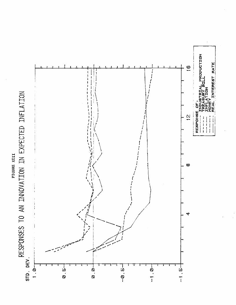
FIG

UR

E X

III

ST

D.

DE

V RESPONSES TO AN INNOVATION IN EXPECTED INFLATION

16

1.0'

0.5

Ia.

—1 .ø

—1

4 8

12

rRE

SP

OS

E O

F'

IND

US

TR

IAL

PR

OD

UC

TIO

N

I T

RE

AS

UR

Y S

ILL

I —

— - —

IN

FLA

TIO

N

I —

—.—

- M

ON

EY

R

EA

L IN

TE

RE

ST

RA

TE

__

__

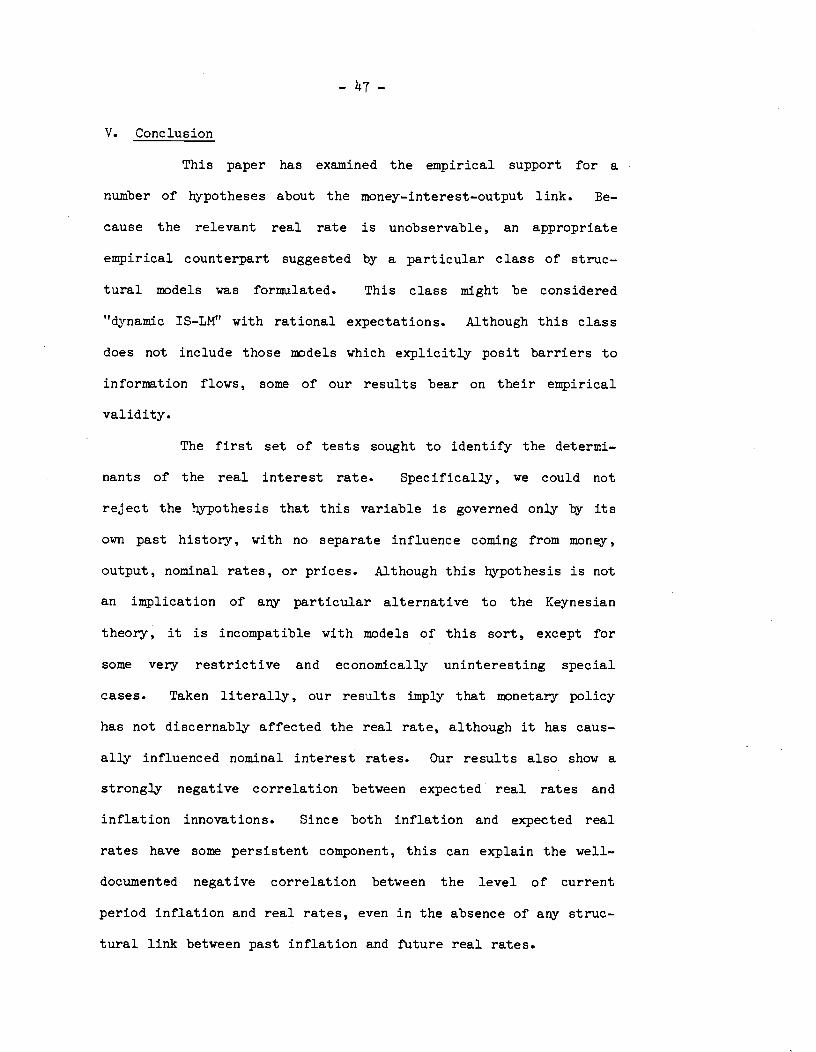
— 147

V. Conclusion

This paper has examined the empirical support for a

number of hypotheses about the money—interest—output link. Be-.

cause the relevant real rate is unobservable, an appropriate

empirical counterpart suggested by a particular class of struc-

tural models was formulated. This class might be considered

"dynamic IS—LM" with rational expectations. Although this class

does not include those models which explicitly posit barriers to

information flows, some of our results bear on their empirical

validity.

The first set of tests sought to identify the determi-

nants of the real interest rate. Specifically, we could not

reject the hypothesis that this variable is governed only ty its

own past history, with no separate influence coming from money,

output, nominal rates, or prices. Although this hypothesis is not

an implication of any particular alternative to the Keynesian

theory, it is incompatible with models of this sort, except for

some very restrictive and economically uninteresting special

cases. Taken literally, our results imply that monetary policy

has not discernably affected the real rate, although it has caus-

ally influenced nominal interest rates. Our results also show a

strongly negative correlation between expected real rates and

inflation innovations. Since both inflation and expected real

rates have some persistent component, this can explain the well—

documented negative correlation between the level of current

period inflation and real rates, even in the absence of any struc-

tural link between past inflation and future real rates.

— I8 —

Our second set of tests found that it is not possible to

filter the observed influence of money and nominal interest rates

on output through expected real rates. This result casts doubt on

the Keynesian transmission mechanism between money and output. A

central new result of this paper is that there is information in

the level of expected inflation for predicting future output which

is not contained in the history of past output or past and future

expected real interest rates. wo explanations for the apparent

predictive content of expected inflation on output have been

advanced. The structuralist interpretation focuses on nonneutral—

ities of various (nonoptimal) institutional nominal rigidities,

but leaves unanswered the causes of changes in inflation. The

other hypothesis argues that output is structurally exogenous to

money and prices, but that new information is first reflected in

expected inflation and interest rates. We find that data to be

surprisingly consistent with this latter hypothesis.

— 49 —

FOOTNOTES

1"The data are from Salomon Brothers, yields are re-

corded on the first trading day of the following month. However,

prior to 1964 Salomon Brothers reports midmonth yields, and after

1977 the data are taken from the U.S. Treasury Bulletin, which

reports yields on the last trading day of the month.

also estimated a number of larger systems including

(not all at one time) inventories, retail sales, real wages, wage

settlements, the monetary base, a stock price index, the uneniploy—

rnent rate, 10—year bond yields, and a trade—weighted index of the

value of the dollar. The qualitative behavior of the output

response to interest rate innovations described above appeared in

every system estimated.

1/Our test is based on a likelihood ratio statistic

generated from the restriction that separate coefficients in

vector autoregressions on two subsamples are equal. The systems

use the variables described in the text and include six lags of

each plus a constant. The two subsamples are 1949:1 through

1971:12, and 1972:7 through 1981:8. The variables in the latter

half are scaled so that residual error variances are the same in

both subsamples. The test follows the procedure described by Sims

(1980b), page 17, to correct for degrees of freedom. The results

of the test were affected little by varying the sample break

between 1966 and 1973.

We interpret this test statistic with extreme skepti—

cism, however, because of its low observation—to—parameter ratio

in this application and the asymptotic nature of the distribution

— 50 —

theory on which it is based. To judge the applicability of this

distribution theory to our test, we created artifical data by

simulating the system with fixed coefficients (and normally dis-

tributed errors with covariances) equal to those estimated using

the entire sample. That is, we generated data under conditions in

which the null hypothesis is known to be true. Under these condi-

tions our test procedures led to statistics which rejected the

null hypothesis eight times out of ten at the .01 significance

level. One of the ten statistics was 185.8, larger than the

180.92 we observed on the actual data.

-JThe expected inflation projections use data beginning

in 1948:1. The first projection is made in 1955:1 and projections

are made each period through the end of 1981. The projections are

made out—of—sample in order to better measure the expectations of

agents who do not benefit from the hindsight afforded by in—sample

projections. We take these expectations as data and then fit a

vector autoregressive representation. We follow this procedure in

order to avoid the prescient expectations which are embodied in

the in—sample projections of a vector autoregression fit directly

to the observable data. For equations such as ours with many free

parameters, the forecast errors generated by in—sample fit may be

substantially smaller than out—of—sample errors.

-JThe quarterly real rate is based on the IF, CPI, and

Ml observations for the third month of each quarter. The nominal

rate is the end—of—quarter value for Treasury bills with three

months to maturity, BILLS3. Inflation expectation projections are

generated in the same manner as described previously except only

two lags of the quarterly data were used.

— 51 —

The six.-month real rate is based on monthly data and the

same projection equations except that the one—month nominal rate

is replaced with a six—month to maturity Treasury bill rate,

BILLS6. The chain rule of forecasting is then used to project

inflation expectations six months forward.

The ex post one—month real rate is the nominal rate,

BILLS1, minus the actual inflation at annualized rates from the

current to the next month.

JWe should caution the reader that the innovations

discussed in this section are defined relative to the four vari-

ables in the vector autoregression. In particular, these innova-

tions are based on projections on lagged expected inflation, (or

equivalently real rates) but not on lagged actual inflation.

Asymptotically this does not matter since if the coefficients are

fixed and known, then for given initial conditions the observa-

tions on expected inflation and other variables are sufficient to

determine the actual inflation rates.

..L"We view the similarity of these results with the

earlier results as evidence that the use of in—sample expectations

is not likely to be misleading, and we continue with this approach

in the next section. The unrestricted vector autoregressions used

here are described fully in the next section as Alternative C for

monthly data and Alternative B for quarterly data.

— 52 —

Bibliography

1. Barro, Robert J. (1976) "Rational Expectations and The Roleof Monetary Policy," Journal of Monetary Economics 2, 1—32.

2. ____________ (1977) "Unanticipated Money Growth and Unemploy-ment in The United States," American Economic Review 67,2, 103—115.

3. _____________ (1980) "A Capital Market in an EquilibriumBusiness Cycle Model," Econometrica 48, 6, 1393—1417.

4. Doan, Thomas (1980) "Maximum Likelihood Tests for the Pres-ence of a Block Causal Ordering," University of Minne-sota, mimeo.

5. ____________, and Robert Litterman (1980) User's Manual RATSVersion 4.0, VAR Econometrics.

6. Fama, E. F. (1975) "Short Term Interest Rates as Predictorsof Inflation," American Economic Review 65, June, 269—82.

7. ____________, and M. R. Gibbons (1980) "Inflation, RealReturns and Capital Investment," August, unpublished,University of Chicago.

8. Grossman, S., and L. Weiss (1980) "Heterogenous Informationand the Theory of the Business Cycle," Cowles FoundationDiscussion Paper#558, Yale University.

9. Lucas, R. E. (1972) "Expectations and the Neutrality ofMoney," Journal of Economic Theory, 103—24.

10. Misbkin, F. (1980) "The Real Rate: An Empirical Investiga-tion," NBER Working Paper #622.

11. Revankar, Nagesh S. (1974) "Some Finite Sample Results in theContext of Two Seemingly Unrelated Regression Equations,"Journal of the American Statistical Association 69, 345,187—190.

12. Sargent, Thomas T. (1978) "Estimation of trnamic Labor DemandSchedules Under Rational Expectations," Journal ofical Econor 86, 6, 1009—1044.

13. Sims, C. A. (1980) "Comparison of Interwar and Postwar Cy-cles: Monetarism Reconsidered," American Economic Review70, 250—257.

14. _____________ (1980a) "International Evidence on MonetaryFactors in Macroeconomic Fluctuations," unpublished.

— 53 —

15. _____________ (1980b) ttMacroeconomics and Reality," Econo—xnetrica 18, i—1t8.

16. Summers, L. (1981) "Inflation, Taxation and Corporate Invest-ment," unpublished, M.I.T.