NBER WORKING PAPER SERIES

$2.00 GAS! STUDYING THE EFFECTSOF A GAS TAX MORATORIUM

Joseph J. Doyle, Jr.Krislert Samphantharak

Working Paper 12266http://www.nber.org/papers/w12266

NATIONAL BUREAU OF ECONOMIC RESEARCH1050 Massachusetts Avenue

Cambridge, MA 02138May 2006

We would like to thank Gordon Hanson, Craig McIntosh, Jim Poterba, Andrew Samwick, Tom Stoker andseminar participants at the University of California, San Diego and the NBER Public Economics ProgramMeeting for useful comments. Evan Chan provided excellent research assistance. Generous support fromMIT Center for Energy and Environmental Policy Research is gratefully acknowledged. The views expressedherein are those of the author(s) and do not necessarily reflect the views of the National Bureau of EconomicResearch.

©2006 by Joseph J. Doyle, Jr. and Krislert Samphantharak. All rights reserved. Short sections of text, notto exceed two paragraphs, may be quoted without explicit permission provided that full credit, including ©notice, is given to the source.

$2.00 Gas! Studying the Effects of a Gas Tax MoratoriumJoseph J. Doyle, Jr. and Krislert SamphantharakNBER Working Paper No. 12266May 2006JEL No. H2

ABSTRACT

There are surprisingly few estimates of the effect of sales taxes on retail prices, especially at the firmlevel. Further, along both sides of a state border, a change in one state’s sales tax can shed light onthe nature of competition, as a subset of firms effectively experiences a change in its marginal cost.This paper considers the suspension, and subsequent reinstatement, of the 5% gasoline sales tax inIllinois and Indiana following a temporary price spike in the spring of 2000. Earlier laws set thetiming of the reinstatements, providing plausibly exogenous changes in the tax rates. Using a uniquedataset of daily, gas station-level data, retail gas prices are found to drop by 3% following thesuspension, and increase by 4% following the reinstatements. After linking the stations to drivingdistance data, some evidence suggests that the tax increases are associated with higher prices up toan hour’s drive into neighboring states.

Joseph J. Doyle Jr.MIT Sloan School of Management50 Memorial DriveCambridge, MA 02142and NBERjjdoyle@mit.edu

Krislert SamphantharakGraduate School of International Relations and Pacific StudiesUniversity of California, San Diego9500 Gilman DriveLa Jolla, CA 92093krislert@ucsd.edu

2

1. Introduction

Gasoline prices are particularly visible, and when they spike there are often calls

to reduce or eliminate gas taxes [Berryman, 2005; Sanger, 2006]. State and federal taxes

add forty cents to the average gallon of gasoline in the United States, resulting in over $8

billion in tax receipts each year [EIA, 2005]. For a tax moratorium to reduce prices it is

necessary to estimate the pass-through rate—the proportion of the tax paid by

consumers—at least in the short run. Further, the each state’s moratorium provides an

opportunity to study the effect on competition when one set of firms receives a tax

change while others in the same market do not.

The theory of tax incidence suggests that sales and excise taxes should be fully

passed onto consumers in competitive markets with constant marginal costs.1 Less than

‘full shifting’ is expected in markets with increasing marginal costs, while the pass-

through rate may be less than, or greater than, one-hundred percent in markets that are

less competitive. In addition, tax increases in one state may lead to higher prices across

the border as stations there face greater demand.

Despite the attention paid to tax incidence, surprisingly little empirical work has

estimated the effect of sales taxes on prices [Poterba, 1996; Besley and Rosen, 1999;

Kenkel, 2005]. This paper studies a moratorium on gasoline sales taxes in Illinois and

Indiana during the summer and fall of 2000 to estimate the effect of tax changes on retail

prices and cross-border competition. Using a unique data set of daily prices at the gas-

station level, linked with census and geographic data including driving distance to the

1 Kotlikoff and Summers [1987] and Fullerton and Metcalf [2002] offer detailed reviews.

3

state border, prices are compared with neighboring states before and after the tax

changes.

The tax moratorium offers four main advantages. First, the reinstatement of the

gasoline tax in these states offers a plausibly exogenous change in the tax rate. In

Indiana, a 1981 law allowed the tax suspension to last only 120 days, while Illinois set

the tax repeal expiration to the potentially arbitrary time of the end of the year. While the

dates of the reinstatements were known and could have increased demand (and prices)

just prior to the tax increases, the lack of a pre-existing trend in price differences across

states at the time of the reinstatements suggests that the reinstatements were not related to

market conditions.

Second, the repeal and subsequent reinstatements allow estimates of the pass-

through rate for both decreases and increases in the tax. Similar estimates of the effect of

the tax on retail prices would suggest that the price changes are tied to the tax rate

policies. The comparisons also provide a test for asymmetry in the response to changes

in stations’ marginal costs, as the downward price adjustment may be stickier than the

upward adjustment [Borenstein, Cameron and Gilbert, 1997].

Third, while the short-run nature of the policy change does not inform long-run

effects, it does provide a way to study the extent of the geographic market for gasoline.

In particular, the station locations can be considered fixed in this context.

Last, gasoline is a homogeneous product where quality differences across space

are minimized when studying the pass-through rate of sales taxes across retailers. The

key differentiation in the market would appear to be location, a subject we consider in

detail below.

4

The results suggest that retail gas prices drop by 3% following the elimination of

the 5% sales tax, and increase by 4% following its reinstatement. While the point

estimates suggest some asymmetry in response to the tax decrease versus the tax increase,

equal responses cannot be rejected in the data. Further, full pass-through can be rejected

in response to the tax decrease in both states and the tax increase in Illinois. In terms of

distance from the border, the tax increase in Indiana is associated with higher prices up to

an hour away from its border, though the evidence is mixed for the Illinois reinstatement.

Results are similar across a number of robustness and specification checks. For example,

the effects are similar across cities and neighborhoods with different numbers of

competitors. Meanwhile, pass-through rates are slightly higher in richer neighborhoods,

consistent with less-elastic demand in those areas. As a whole, the results suggest that

pass-through rates are between sixty and eighty percent for retail gasoline in the short

run.

The structure of the paper is as follows. Section two briefly provides

background on the reasons for the tax repeals and how they were conducted, as well as a

review of the related literature to place the current results in context. Section three

describes the data and presents mean comparisons of ZIP code characteristics across the

comparison groups. Section four presents the empirical model and results. A number of

specification and robustness tests are also described. Section five concludes.

2. Background and Related Literature

2.1 Background

5

In the spring of 2000, gasoline prices rose sharply in the Midwest. Figure I shows

the average daily price of regular unleaded gasoline in Chicago, the rest of Illinois,

Indiana, Kentucky, and the other states that are neighbors to Illinois and Indiana

(Wisconsin, Iowa, Missouri, Ohio and Michigan, see map in the Appendix). Average

prices spiked to $2.11 per gallon in Chicago, and $1.78 in Indiana on June 19, a very

high, and politically unattractive, price at the time (though welcome in the spring of

2006). Much was written about the increase in gasoline prices at the time, as evidenced

by at least four reports investigating the cause of the price spikes including an

investigation by the Federal Trade Commission [Conrad, Howard, and Noggle, 2000;

Shore, 2000; Martin, 2001; FTC, 2001]. The spike has been attributed to short supplies

of refined gasoline in anticipation of a change in the reformulation required of refineries,

along with unexpectedly high demand [FTC, 2001], though Figure I shows that the price

spike was fairly short lived.

In response to the spike, on June 20, 2000, the governor of Indiana used the power

granted under a 1981 statute to declare an energy emergency, allowing him to suspend

the five percent sales tax on gasoline for 60 days, with a possible extension for another 60

days. He announced that the suspension would begin on July 1st, with the sixty day

timeframe. He later extended the suspension three times: on August 22nd changing the

end date to September 15th, on September 13th extending the suspension until September

30th, and on September 28th allowing the suspension to run its 120 day course.2 This

was an election year in Indiana, and the Indiana governor was criticized for continuing

2 On October 25th, the governor made known that the sales tax would be ending. State press releases noted that the sales tax would be reinstated at midnight on October 25th, though subsequent press reports noted the price jump at the 120 day mark (The Indianapolis Star, November 8, 2000). Further, the clear jump in prices occurred at the 120 day mark in the data. Price differences between Indiana and neighboring states did not change on September 1st, 15th, or 30th. The timing of the effect is discussed further below.

6

the sales tax suspension in August and September when prices had already fallen (see

Figure I). The political justification for the extensions, and the 120 day cutoff set by the

1981 law, suggest that the tax reinstatement was not tied to market conditions.

Meanwhile, the excise tax is connected to highway funding and was not allowed to be

suspended without legislative approval.

In Illinois, the legislature responded by passing a bill on June 28th suspending its

five percent sales tax on gasoline, set to begin on July 1st as well. The moratorium in

Illinois was set to end six months later on January 1, 2001. Of the neighboring states,

only Michigan had a sales tax to consider suspending, and while there was talk of a

suspension it did not occur.

The effect of the repeal on gasoline taxes was questioned at the time. While the

Illinois law required gasoline retailers to post a notice that the gasoline tax had been

suspended, the governor of Illinois, George Ryan, noted: “There is no guarantee in a

free-market economy that prices will go down, but I believe that the political and public

pressure applied by the roll back of the sales tax will help force prices down.” [Ryan,

2000]. A subsequent appraisal showed that prices had fallen following the tax

suspension, though the investigation did not attempt to disentangle the effect of the tax

suspension with the falling wholesale prices at the time [Conrad, Howard, and Noggle,

2000].

2.2 Related Literature

7

Poterba [1996] reviews the early empirical literature on sales tax incidence and

argues that there has been relatively little empirical work on the incidence of sales taxes.3

Further, the evidence has been mixed with regard to incomplete, full, and over shifting of

taxes on retail prices. Poterba [1996] analyzes city-specific clothing price indices for

eight cities during 1947-77 and fourteen cities during 1925-39. Retail prices rose by

approximately the amount of the sales tax for the post-war period but only by two-thirds

during the Depression years. Besley and Rosen [1999] use quarterly data for 12

commodities (such as bananas, bread, milk and Big Macs) in 155 cities during 1982-90.

Their model includes city fixed effects to test the effect of changes in tax rates on retail

prices. While the pass-through rates for some commodities are estimated to be close to

100%, their results also suggest that several commodities have what has been labeled

overshifting: pass-through rates of well over 100%. Kenkel [2005] recently studied the

effect of tax hikes on the price of alcoholic beverages in Alaska. His interesting results

suggest that alcohol taxes are more than fully passed through to beverage prices.

In the case of gasoline prices, the prediction of the pass-through rate is

ambiguous, as the market for retail gasoline is usually characterized as imperfectly

competitive due to the spatially-differentiated nature of the market [Verlinda, 2004].

Other factors that determine local market demand elasticity such as demography,

household income, and means of commuting are also likely to affect the pass-through

rate.

In terms of the empirical literature on gasoline taxation, Chouinard and Perloff

[2002] used a monthly panel of the 48 US contiguous states and the District of Columbia

3 Early studies include Brown [1939], Due [1942] and Bishop [1968].

8

between 1989 and 1997 to estimate a reduced-form model of gasoline prices. Among

other results, they find that tax variations and market power (measured by mergers)

contribute substantially to geographic price differentials. Using a model with state fixed

effects, they also find that 50% of federal excise tax incidence is passed on to consumers,

75% of state ad valorem taxes like those studied here are passed on to consumers, and

nearly all of the state excise taxes are passed on to consumers. Meanwhile, wholesale

prices appear unaffected by changes in state tax rates. In another paper, Chouinard and

Perloff [2004] also find that state-specific taxes fall almost entirely on consumers,

especially in states that use relatively little gasoline and have lower elasticity of supply.

While the potential endogeneity of the timing of the tax changes was not explored, the

results are consistent with less than or full shifting of taxes in gasoline markets.

Alm, Sennoga, and Skidmore [2005] also consider a panel of monthly gasoline

prices for the fifty U.S. states and estimate the effect of changes in excise taxes on retail

prices using a model with state fixed effects. They find that the excise tax is fully passed

on to consumers within the first month of a tax change, with no effect on retail prices of

the one-month lag in the tax level. This is consistent with the results presented below

that comparisons just before and after the tax changes likely capture the full (if short-run)

effects on retail prices. The paper also notes the potential impact of spatial competition

by comparing the results for urban versus rural states. They find that the pass-through

rates slightly smaller in rural states, where stations are thought to be more widespread. In

addition, they test whether prices respond differently to excise tax increases and

decreases and do not find an asymmetry in the response. Like the Chouinard and Perloff

papers, the timing and potential endogeneity of the excise tax changes were not

9

considered, and aggregate data precluded the study of the spatial effects of the tax

changes at the station level.

Our analytical framework follows the Chouinard and Perloff reduced form

specification. The demand function for gasoline is given by Q = D(p, X), where p denotes

the gas price and X represents exogenous demand shifters. On the supply side, the

reduced-form marginal cost function is MC(t, W), where t is the tax parameter and W

represents cost shifters. Profit maximization implies that the marginal cost of a firm

equals its marginal revenue. Therefore, we have p = f(t, X, W, Z), where Z consists of the

variables that capture the market power of the firms, which in turn results in price being

different from firms’ marginal revenue.

In the model, the effect of a tax increase on price also depends on demand

conditions, cost structure and market power of the firms. In a perfectly competitive

market, we would expect that the tax would be completely passed through to the

customer when the firms face constant marginal cost, while the pass-through rate is less

than one when they have increasing marginal cost. However, as pointed out by Katz and

Rosen [1985] and Stern [1987], the ‘full tax shifting’ case cannot be generalized as the

upper bound when the market is not perfectly competitive. In that case, the pass-through

rate of the tax could be either below or above 100%, depending on the elasticity of

demand. For example, in the case of isoelastic demand, the pass-through rate in a market

with an oligopoly is more than 100%, and will be still greater in monopolistic

competition if the elasticity of demand is less than one.

10

The gas tax repeal studied here may impact competition across state borders as

well. A decrease in the state tax rate may lower prices for that state’s drivers, as well as

drivers from neighboring states if stations across the border are part of the same market.

Previous evidence suggests that consumers should not be willing to travel very far

to save on gasoline, despite anecdotal accounts of price shopping. Manuszak and Moul

[2005] use local tax differences to study the static trade-off between price and traveling.

Using data from the Chicagoland area (Chicago, Cook County, Will County and

Northwest Indiana) in July 2001, they find that a typical Chicagoland consumer must

save $0.55 per fill-up in order to travel to a station an additional mile away. This

suggests that traveling for cheaper gas prices is not cost effective.

Nevertheless, the market size is likely reflected by commuting patterns.

Commuters, and interstate commercial drivers, do not require additional travel to find

lower prices. These drivers may delay their purchase to find the station with cheaper

prices along their routes and may extend the size of the market for gasoline.4 The

analysis below considers the effect of the tax changes on competition across state

borders, which will also provide some evidence on the appropriateness of using

neighboring states as comparison groups.

There are some studies that look at cross-border competition in other industries.

For example, Coats [1995] studies the effects of state cigarette taxes in the US and finds

that about fourth-fifths of the sales response to state cigarette taxes is due to cross-border

sales. Sumner [1981] and Ashenfelter and Sullivan [1987] also use cross-state

differentials in cigarette excise taxes to study the extent of market power in the industry.

4 The US Census metropolitan statistical areas are defined by commuting patterns for largely this reason.

11

Further, the effects of a state’s spending policies on other states have been considered as

well (see, for example, Case, Hines, and Rosen [1993]).

The tax changes studied here may affect prices across time as well as across

space. For example, consumers may delay their purchase of gasoline just prior to the tax

suspension, or increase their purchase of gasoline just prior to the tax reinstatements.

This may lead to lower prices just prior to the suspension and higher prices prior to the

reinstatement. Such changes in prices are explored below.

One advantage of the temporary nature of the suspension is that it allows a study

of the extent of the geographic market for gasoline taking the location of the stations as

given. In equilibrium, differences in taxes across jurisdictions simultaneously determine

not only the gas price in each station, but also dictate the location of the gas stations

across geographic areas. The temporary tax changes are not likely to change the location

decisions of the station owners, or the decision for new stations to enter the market. As a

result, the effect of the tax changes should be reflected mainly in the gas prices, as they

change the static trade-off between price and traveling costs across borders for gasoline.

3. Data Description

The analysis uses a unique dataset of daily gasoline prices at the station level.

These prices are collected by Wright Express Financial Services corporation, a leading

provider of payment processing and financial services to commercial and government

car, van and truck fleets in the United States. Their Oil Price Information Service (OPIS)

provides retail gasoline prices for up to 120,000 gasoline stations each day using

information from its credit card receipts. These data are sold to firms aiming to minimize

12

fuel expenses, as well as the American Automobile Association. The fleet card

separately identifies gasoline purchases from other items (such as food) and records the

per-gallon price. One advantage of the data is that measurement error should be

minimized, as the prices are recorded electronically from the charge cards.5 Prices for

regular unleaded will be the focus of the analysis below.

The OPIS also includes wholesale prices for each station. This is a rack price—

the price at the terminal—from the nearest refinery that produces the formulation of

gasoline used by the station. Branded gasoline, such as Shell or Mobil, are sold through

distributors called “jobbers”, and the OPIS records the terminal price from each of these

distributors as well as the standard rack price charged to unbranded stations. This

measure will differ from the stations’ actual wholesale price in that it does not include

volume discounts or delivery charges. The percentage change in the wholesale price over

time should fairly accurately reflect changes in the wholesale price, however.

Figure I showed that the price spike was particularly severe in Chicago, and

noticeably less so in Kentucky. For greater comparability, the main analysis will exclude

the Chicago-Naperville-Joliet, IL, IN, WI Metropolitan Statistical Area, as well as

Kentucky, though the results are similar when these areas are included as shown below.

Stations in Illinois, Indiana, and five neighboring states: Michigan, Ohio, Missouri,

Iowa, and Wisconsin are compared, where roughly 6,000 stations are surveyed each day.

The data has some missing days, however, especially on weekends and holidays. For

example, there are no observations during July 1- July 4, and few observations right at

January 1. Instead, the main analysis will focus on prices just before and after the tax

5 Further information on the methodology is available at http://opisnet.com/methodology.asp, as well as www.senate.gov/~gov_affairs/ 042902gasreport/appendix1.pdf.

13

changes as allowed by the data, using two days before and after to increase the number of

stations observed. For the July tax repeal, June 27 and 28 are compared to July 5 and

July 6; October 26 and 27 are compared to October 31 and November 1 for the Indiana

reinstatement; and relatively fewer observations for December 29 and 30 are compared to

January 2 and 3 for the Illinois reinstatement. Specifications that consider longer time

frames and flexible treatments for time variation are estimated as well.

The OPIS data also include the street address of each station. US Census of

Population data at the ZIP code level in 2000 are used to compare the groups and to

control for neighborhood characteristics such as the age, race, and educational

composition, median household income, population, and commuting behavior. The US

Gazetteer ZIP Code file from the US Census was collected, which includes the area of the

ZIP code and its latitude and longitude. In addition, the 2000 US Census ZIP Code

Business Patterns database records the number of gasoline stations in each ZIP code,

which will be used as a control on the local competitive environment. Maps were used to

identify those ZIP codes with an interstate highway as a measure of access to gasoline

stations that are effectively closer in terms of travel times.

The address data also allows an estimate of the distance from the station to the

state border. First, ZIP codes that comprise the state borders were identified using ZIP

code maps. Then, for stations in Illinois/Indiana, the minimum driving distance (in

minutes) from each ZIP code to a neighboring-state ZIP code was calculated using

software from Mapquest™. This data source has the advantage of calculating distances

as consumers would travel from one area to the next, as opposed to distances calculated

along a straight line. For stations in the neighboring states, the distance from each station

14

to the nearest Illinois or Indiana ZIP code was also calculated. This allows a comparison

of stations near the Illinois/Indiana border, as well as those farther from the border, to test

the effect of the Illinois/Indian tax changes on stations in neighboring states.

One potential limitation of the pricing data is that it may oversample stations used

by consumers who travel extensively. The coverage appears fairly complete in the

Midwest, however. When comparing stations in the pricing survey and those in the

Census data, the median ZIP code had three quarters of the stations surveyed (estimates

across ZIP codes with different coverage rates will be compared below). Further, the

surveyed stations include many unbranded gasoline stations, and over a third of the

stations surveyed are in ZIP codes with no interstate, suggesting that the coverage is not

limited to the most densely populated areas.6

Table I describes the prices and variables used as controls and demonstrates that

the comparison groups are similar. The sample considered is for the July tax repeals.

One difference is in terms of average gas prices: retail prices were ten cents cheaper in

Indiana/Illinois, partly because prices had declined already prior to the moratorium and

partly because Chicagoland is excluded here. Wholesale prices, meanwhile, were four

cents cheaper per gallon. Federal and state excise taxes make up much of the difference

between wholesale and retail prices. These excise taxes are constant throughout the time

period, and the state sales tax is applied to the after-excise-tax price.7

6 To explore the types of ZIP codes that have better coverage in the pricing sample, the ZIP code count of the number of stations in the sample was regressed on the observable characteristics in Table I. The main result is that more populous ZIP codes are associated with more stations surveyed, even after controlling for the number of stations in the Census data. Results are compared across ZIP codes with different coverage rates below. 7 According to the OPIS, stations are estimated to earn margins of less than five cents per gallon, with the remaining costs including distribution from terminals to stations, franchise fees, rents, wages, utilities, supplies, equipment maintenance, environmental fees, licenses, permitting fees, credit card fees, insurance, depreciation, and advertising.

15

In terms of ZIP code characteristics, the differences are statistically significant

given the large number of observations, but the neighborhoods appear fairly similar. For

example, the Illinois/Indiana ZIP codes have median household incomes are $42,000

versus $43,000 in the neighboring states. The commuting patterns were computed for all

workers in each ZIP code, and stations in both comparison groups are located in ZIP

codes with an average of 82% of workers who drive to work alone. Meanwhile,

commute times are nearly identical. The population is somewhat smaller in the

Illinois/Indiana ZIP codes (19,000 versus 21,000). One reason for the similarity in the

ZIP codes is the exclusion of Chicagoland. When stations in the Chicago MSA were

included, the Illinois/Indiana ZIP codes tended to have much higher gasoline prices, were

more urban, higher income, younger, and more likely to have residents using public

transportation.

4. Empirical Model and Results

All results in the paper are presented with respect to three time periods: the

summer of 2000 when stations in Illinois/Indiana are compared to neighboring states; the

fall of 2000 when Indiana is compared to its neighboring states including Illinois; and the

winter of 2000/2001 when Illinois is compared to its neighboring states including

Indiana.

4.1 Main Results

The main results are in Figure II, where the points represent the difference in

average log retail prices between Illinois/Indiana and neighboring states at each date and

the solid lines are the result of a local linear regression of these differences against time.

16

The models were separately estimated before and after the tax changes, and the size of

the discontinuity at the time of the tax change is a difference-in-difference estimate of the

effect of the tax change on retail prices.8 Note that these models do not control for

differences in wholesale price changes as will be discussed below.

Figure IIa reports the results for the summer of 2000. One feature is the

downward trend in the difference in gas prices prior to the moratorium. Recall that there

was a spike in the spring of 2000, and the legislation appears to be dealing with a

problem that was already ameliorating—a chief criticism of the tax changes [Martin,

2001]. This pre-reform trend in price differences suggests that the difference-in-

difference estimate may reflect other changes in the market, and may overstate the effect

of the tax change on retail prices—the price differences may have declined without the

tax change. The difference does appear to level off prior to the tax change, however, and

the difference-in-difference estimate implied by the local linear regressions is a reduction

in retail prices of 2.7 log points, or approximately 2.7%, following the suspension of the

5% sales tax.9

Figures IIb and IIc compare the differences in retail prices against time when the

gas taxes are reinstated. Figure IIb representing the Indiana reinstatement in October

shows the average differences are constant before and after the tax changes, with a

discontinuity right at the time of the reform, suggesting that the sunset provision provides

a plausibly exogenous change in the tax rate. The price differences jump at the end of

8 Results shown have a bandwidth of 7 days. Results are slightly smaller with a bandwidth of 14 days, with difference-in-difference estimates of -1.8%, 4.1%, and 2.0%. OLS estimates with flexible time frames are discussed below. 9 The distinct jump in prices suggests that the effects happened right away, as opposed to consumers increasing demand just before the tax increases, or stations reacting slowly over time. In terms of the stations’ responses, an S-shape in the jump would be expected if some stations responded immediately while others waited [Caballero et al., 1995]. Responses by day are considered in more detail below.

17

November, but this is due to a temporary increase in retail prices in Illinois not

experienced by Indiana or its other neighboring states. Figure IIc shows that the data are

noisier at the end of the year, partly reflecting the smaller sample sizes at that time.

While the end dates were not chosen to reflect concerns about market conditions,

the announced end date may affect purchasing habits prior to the tax increase, and with

intertemporal substitution the effect of the tax change may be underestimated. The raw

data suggest that prices do not follow this pattern in July or October, and the slight rise in

prices prior to the reinstatement in January is not found when wholesale prices are

controlled, as discussed below. This suggests that the comparison of prices before and

after the reform provide a useful estimate of the effect of the tax change on retail prices.

The local linear regression estimates suggest that Indiana’s retail price increased

by 4% relative to neighboring states at the time of the 5% tax increase, while Illinois’s

retail price rose by 2.8% at the time of its reinstatement.

These raw comparisons do not take into account differences between

Illinois/Indiana and neighboring states, especially potential differences in wholesale

prices changes. To test the effect of the tax changes on retail prices controlling for these

factors, the following model is estimated for station s selling brand b at time t:

(1)

sbtbsst

ts

tssbt

εδγγγ

γγγ

+++++

++=

X)PriceWholesaleln(ReformPost*)Indianaor Illinois(1

ReformPost)Indianaor Illinois(1)PriceRetailln(

54

3

210

where 1(Illinois or Indiana)s is an indicator that the station is in Illinois or Indiana for the

July time period, Indiana for the October comparison, and Illinois for the January

comparison; Post Reformt is an indicator that the gas price is observed after the tax

change; and Xs is a vector of the station’s ZIP code characteristics described in Table I.

18

Brand fixed effects are also included, as decisions at the brand level may affect

the reaction of prices to the change in taxes.10 One issue is that brands primarily in one

state will be nearly collinear with the indicator for Illinois or Indiana. As a result, the

indicators for major brands that make up at least five percent of the station observations

in both the treatment and comparison groups are included. These major-brand stations

account for 60% of the observations. Results are nearly the same when brand fixed

effects for all stations are included while restricting the data to those brands observed in

both comparison groups, but including the indicators for only the major brands allows the

use of all the stations.

Table II reports the results of models with and without controls. Again, the

estimates are broken into three time periods: just before and after July 1, October 31, and

January 1. Column (1) includes no controls and retail prices are estimated to fall by

roughly 3.5% in July, and increase by 3.9% in October and 2.7% in January. These

estimates imply pass-through rates of 70%, 78%, and 54%, respectively.

Column (2) includes the wholesale price which serves to control for differential

changes in the costs of the stations at the time of the reform. (The potential effect of the

tax reform on wholesale prices is explored below.) The estimates decrease to 2.9% in

July, remain about the same in October at 4.0%, and increase in January to 3.6%.

The neighborhood characteristics may differ across the comparison groups as

well, which may affect the response to shocks at the time of the reform. When the

control variables listed in Table I and brand indicators are included, the results are

essentially unchanged as shown in Column (3). This confirms the conclusion of Table I

10 Hastings [2004] studied the conversion of independent gasoline stations into branded gasoline stations and found evidence of consumer brand loyalty which can affect the price response to the tax changes.

19

that the Illinois and Indiana neighborhoods are similar to those in the neighboring states,

especially with the exclusion of Chicagoland, as well as the ability of the difference-in-

difference estimate to control for time invariant differences across the comparison

groups.

The results are similar to the response of retail prices to wholesale price changes.

When data from all of the states considered here from April 1, 2000 to March 31, 2001

were considered, a 5% increase in a station’s wholesale price is associated with a 3%

increase in its retail price. This estimate was stable to the inclusion of control variables

and station fixed effects.

The point estimates are also consistent with an asymmetry in response to marginal

costs increases versus decreases [Borenstein, Cameron, and Gilbert, 1997]. While the

equality of response to the repeal and subsequent reinstatements of the tax cannot be

rejected, the point estimates do suggest that the fall in prices is somewhat smaller than the

increase in response to tax changes. Meanwhile, the full shifting can be rejected for July

and January, though not in October.

Of the control variables, the signs of the associations are generally as expected

(see Appendix Table A1 for complete results). For example, log wholesale prices are

positively associated with log retail prices. Income is positively associated with prices,

possibly reflecting demand and cost of land. The fraction of the ZIP code workers who

carpool is positively associated with gasoline prices, likely reflecting the decision to

carpool both in high gas price areas and around congested cities again with high land

costs. The fraction of workers with long commutes is negatively associated with retail

prices in July and January, possibly as they increase the number of competitors to include

20

gasoline stations along the major commuting routes. Last, the brand fixed effects suggest

that brands earn a premium, with BP and Citgo prices tending to be 2% higher than

unbranded stations, and Mobil and Shell tending to be 3% higher.

4.2 Wholesale Prices

The previous discussion has restricted attention to the retail gasoline market and

controls for wholesale prices in an attempt to compare stations with similar marginal

costs. If wholesale prices were affected by the tax reforms, then the difference-in-

difference estimates would be affected as well. For example, in July when wholesale

prices and taxes are falling at the same time, the estimates would be smaller in absolute

value as the wholesale price control variable soaked up some of the effect of the reform.

Table II showed that the estimate did decrease in July when the wholesale price control

was introduced, though the estimates were stable in October and increased in January.

Column (4) of Table II further investigates the effect of the tax reforms on

wholesale prices. The model is similar to those above, but with log wholesale price as

the dependent variable. The difference-in-difference estimates reveal small decreases in

wholesale prices at the time of the tax changes, including a 1.4% drop in January at the

time of the Illinois reinstatement compared to its neighboring states. The lack of a

significant effect of sales tax changes on wholesale prices suggests that they can serve as

controls for differential costs across the comparison groups. The result is also consistent

with the prior estimates that the tax incidence does not seem to pass on to wholesalers in

the market for gasoline [Chouinard and Perloff, 2004].

4.3 Competition across Borders

21

One question that arises when using neighboring states as a comparison group is

whether or not they were affected by the reforms in Illinois and Indiana. The effect of the

tax change on border competition can also yield insights into cross-border tax incidence

and the extent of the geographic market for gasoline. If the border stations and

consumers along the border (including drivers commuting across the border) respond to

the tax change, we would expect smaller difference-in-difference estimates at the border.

The stations in the treated states would be under less pressure from the cross-border

competitors to pass along the tax savings, and the stations just across the border would be

under more pressure to match any price declines.

To test the effect of the tax change at different distances from the border, stations

were categorized by their distance in five minute intervals from the Illinois/Indiana

border (0-5 minutes, 5-10 minutes, and so on). For stations in Illinois or Indiana, this is

the traveling time to the nearest border (including Kentucky), while for the neighboring

states this is the distance to the nearest tax reform state. For example, the distance

recorded for stations in Michigan is the distance to Indiana, while the distance recorded

for a station in Indiana is the minimum distance to any neighboring state. Note that, for

the July comparison, Illinois and Indiana are treated as one treated region, so the Illinois-

Indiana border is omitted from the calculation. Some cells had few observations, so the

analysis was restricted to cells with at least 10 stations in each of the comparison groups.

This results in few observations far from the border, especially in January.

In each of these cells, the average before-after price difference was calculated

separately for Illinois/Indiana stations and the set of stations in neighboring states. The

22

difference between these price changes was then calculated for each five-minute interval

from the Illinois/Indiana border.

Figure III presents a local linear regression of these price changes against distance

from the Illinois/Indiana border. 11 The horizontal axes in each of the panels are the five-

minute intervals from the border. One regression shows the difference in average log

retail prices before and after the reform in Illinois/Indiana; a second shows the before-

after difference in the neighboring states; and the third is the difference between these

two, representing the difference-in-difference estimate comparing stations that are a

similar distance from the Illinois/Indiana state borders.

In July, the raw data provide little evidence of an effect on border competition,

with larger difference-in-difference estimates (in absolute value) closer to the border.

Not controlling for other observable characteristics, the price drops roughly 14 percent in

the Illinois/Indiana region after the reform regardless of distance to the borders. In the

neighboring states, the prices drop roughly 10 percent seventy minutes and more from the

border, though less of a decline is seen closer to the tax reform states. This leads to a

difference-in-difference estimate that varies from -7% at the border to -5% farther from

the border.

For the reinstatements, the raw comparisons do reveal smaller difference-in-

difference estimates closer to the border. In October, the price increase in Indiana is not

related to distance to the border, although the neighboring states have smaller price

declines near the border compared to stations farther from the treated states. The

estimated difference-in-difference therefore increases from 3.7% at the border to an

estimated 6.9% ninety minutes from the border, dropping to 5.3% one hundred twenty- 11 The estimates use a bandwidth of twenty minutes representing four five-minute cells.

23

five minutes from the border. The large decline at the very end of Figure IIb is partly due

to few observations that far from the border in Indiana.

In January, the raw data are again somewhat mixed: smaller difference-in-

difference estimates are found near the border, but the estimates also decline for when

comparing stations far from the border. While the estimates in July and October had cells

with generally over one hundred stations, the January comparison employs cells with

generally less than fifty stations, especially farther from the border where cells are

typically close to twenty stations. The decline in the effect far from the border in

January, therefore, should be treated with some caution.

One way around the lack of data is to collapse the five-minute intervals into

thirty-minute intervals. In addition, the unconditional comparisons in Figure III do not

take account of potential differences in observable characteristics, such as wholesale

prices or the commuting behavior of residents across space that may affect the results.

Table III reports estimates for a model that considers four regions defined by thirty

minute intervals. Stations over an hour and a half from the border, for example, are

stations within an oval-shaped region in the center of the treated states. For the untreated

states, this is an indicator that the stations are simply far from the treated states.

The models include the same specification as before, but now include the three-

way interaction between each of the three distance categories, 1(Illinois or Indiana), and

Post Reform. The indicators for each distance category and their two-way interactions

with 1(Illinois or Indiana), and Post Reform are also included. The excluded category in

Table III is less than thirty minutes from the border, and the first row reports the

difference-in-difference estimate for this group: -3.5% in July, 3.2% in October, and

24

2.8% in January. Although the preliminary look at the raw data discussed above suggests

smaller estimates for stations farther from the border in July comparison, this is not the

case when the models with full controls are considered. The effect is slightly larger at

thirty to sixty minutes away where summing the coefficient on IL/IN*Post and

IL/IN*Post*1(>=30minutes and <60minutes) reveals a larger difference-in-difference

estimate (in absolute value) of -4.2%. The effect drops slightly at sixty to ninety minutes

away from the border (-3.6%), and is smaller still at stations even farther away from the

border (-2.4%). None of these differences across distance categories are statistically

significant, however.

In October, the effect found in the raw data is present when controlling for

observable characteristics: a difference-in-difference estimate of 3.2% at the border,

remaining flat at 3.3% between thirty minutes and one hour from the border, but

increasing to 4.3% over an hour away from the border. These differences are statistically

significantly different and represent pass-through estimates increasing from 64% to 86%.

In January, the shape of the effect found in the raw data is again evident in the

model with controls, with smaller treatment effects at the border, large treatment effects

sixty to ninety minutes from the border, and smaller effects for stations far from the

border. This decline in the effect far from the border was unexpected and may reflect the

fact that the stations very far from the borders in the comparison states and the stations in

the very middle of Illinois are less comparable. Again, the January results should be

taken with some caution given the relatively smaller sample sizes.

Another way to consider border competition is to test whether the difference-in-

difference estimates are smaller when stations directly across the border from one another

25

are compared. Table IV considers such stations by considering Metropolitan Statistical

Areas (MSAs) that overlap state borders, and all stations along the treated state borders.

MSAs are defined by commuting patterns, which may provide a reasonable market

definition for gasoline consumers.

Column (1) considers Chicagoland, which, up to now, has been excluded from the

analysis due to the lack of comparability among ZIP code characteristics and the size of

the price spike that led to the tax repeal. When stations within the Chicago-Naperville-

Joliet, IL-IN-WI, Metropolitan Statistical Area are considered for July, the model

compares stations in Chicago and Gary, IN, with stations just across the

Illinois/Wisconsin state border. Only three percent of the stations are in the comparison

group, but the estimate suggests a 2.7% decline in prices in the treated stations relative to

the Wisconsin stations—similar to the estimate found in the larger sample. In the

October and January comparisons, there are more stations in the comparison groups:

86% in October and 14% in January. The estimated effect is much smaller in October

(0%) when stations largely in Gary, IN, are compared to Chicago and Wisconsin stations

within Chicagoland. The estimate is somewhat smaller in January (2.7%) when Chicago

stations are compared to the Wisconsin and Indiana stations. The smaller effects found

when the tax was reinstated may reflect differences in the comparison groups, but are

also consistent with smaller treatment effects at the border.

The other border MSAs in July are St. Louis (MO-IL), Cincinnati (OH-IN), South

Bend (IN-MI), Jackson (MO-IL), Davenport (IA-IL), and Burlington (IA-IL).12 For

stations in these overlapping MSAs, a similar model to those presented in Table II was

12 In order to compare the results with previous estimates in Table II, we do not include the MSAs along the Kentucky border in this analysis.

26

estimated with MSA fixed effects. These models use within-MSA variation in the tax

regimes and retail prices to estimate the effect of the tax reforms on retail prices. Table

IV shows that the difference-in-difference estimate is larger in July (-3.6%), slightly

larger in October (4.2%), but smaller in January (1.5%). These estimates provide mixed

evidence that the difference-in-difference estimates are indeed smaller near the border.

A third way to consider the border competition is to compare stations that are just

across the border from one another. To estimate these effects, stations in Illinois/Indiana

that are not in a border ZIP code were excluded, as well as stations outside

Illinois/Indiana that are more than thirty minutes from the border. To compare the

estimates to the main results, Chicagoland is also excluded. Then, an indicator for the

“treated-state ZIP code” was created, which is the ZIP code for a station in

Illinois/Indiana, and the nearest Illinois/Indiana ZIP code for stations outside of

Illinois/Indiana. Table IV presents estimates of models similar to those presented in

Table II, but with treated-state ZIP code fixed effects. The estimates are again larger in

July (-5.6%), but smaller in October (3.1%) and January (1.3%). While the evidence is

again somewhat mixed in terms of the larger effects for July and smaller effects for

October and January, the reinstatements suggest smaller difference-in-difference

estimates for stations that compete along the border compared to stations farther from the

border.

Overall, the results on distance suggest somewhat smaller difference-in-difference

results when analyzed close to the border, especially for the reinstatements. While some

of the evidence is mixed, the results are generally consistent with the effect of the tax

extending across state borders. In particular, the October results appear to be more stable

27

given the relatively larger sample size in October, and the lack of a major driving holiday

that may affect the results. These estimates suggest at 3.2% increase at the border and a

4.3% increase farther from the border. The effect of the tax on retail prices for stations

continues to suggest effects on retail prices of between 3% and 4% following the

suspension and reinstatement of the 5% sales tax.

4.4 Competitive Environment

Another way the pass-through rates can differ is when the market conditions

differ. The temporary nature of the moratorium implies that it should not affect the

structure of the market. To the extent entry barriers are low, each market may be

competitive, whereas zoning regulations may result in high barriers in some locations.

One caveat is that the number of stations likely reflects population density as well, so it is

important to control for population and area while investigating any relationship between

number of stations and the price response to the tax changes.

Table V considers how the difference-in-difference estimates vary across different

types MSAs and ZIP codes defined by the number of gasoline stations. The comparison

reflects how geographic areas with many gasoline stations in the treated states respond to

the tax change relative to areas with similar numbers of gasoline stations in the

neighboring states to control for common trends that may differ by market structure.

MSAs were chosen as they reflect commuting patterns and may reflect the geographic

market, while ZIP codes may reveal differences if markets are much smaller. Results

were similar when only the treated states were considered.

The results suggest little relationship between the number of stations and the

response to the tax change, with a smaller effect found for MSAs with more stations in

28

July and January, but a larger effect found for October. Panel A reports the coefficient on

the three-way interaction between the natural logarithm of the number of gasoline

stations reported to the Census bureau, an indicator for Illinois/Indiana, and an indicator

for Post reform. The models also include the main effects, as well as two-way

interactions between these variables. The first three columns consider the MSA level and

the data are restricted to stations within MSAs, where the average MSA has 544 stations.

The estimates suggest that a doubling of the number of stations decreases the size of the

price decline in July by 0.5 percentage points, an increase in the effect of the tax increase

in November (by 0.4 percentage points), and an imprecisely estimated but small decrease

in January (by 0.1 percentage points). At the ZIP code level, similar estimates are found

in July and October, though the effect is found to be larger in January with an increase in

stations (by 0.7 percentage points).

To explore the idea that the effect may not be log-linear in the number of stations,

panel B breaks the samples into quartiles based on the number of stations. Estimates are

reported for the interaction between IL/IN and Post reform, representing the difference-

in-difference estimate for the excluded quartile: areas with the fewest numbers of

stations. The three-way interactions of IL/IN, Post Reform, and the top three quartiles

are reported to measure the difference in the estimated effect of the tax reform as the

number of stations increase. In July, the average number of stations in each quartile was

36, 113, 441, and 1307 for the MSA comparison and 2, 7, 12, and 20 for the ZIP code

categories.

The results largely mirror the results in Panel A. In July, the number of stations in

the MSA is not related to the price response until the top quartile, when the estimated

29

effect becomes much smaller. It should be noted, however, that only 5% of the stations

in the top quartile are in the treated states in July. The October reinstatement is

associated with an increasing effect with the number of stations, while the January

reinstatement is associated with a slight rise and fall of the response to the tax increase

with the number of stations. At the ZIP code level, no relationship with the number of

stations is found in July or October, while the January reinstatement suggests a rise in the

estimated effect in the third quartile.

The mixed results, coupled with the size of the estimated effects, suggest that the

earlier results are fairly robust to the type of market considered. If markets with many

stations are thought to be competitive, then the robustness of the results across markets

with different numbers of stations is consistent with gasoline markets requiring only a

few stations to be as competitive as those with many more stations.

Market conditions on the demand side may affect the response to the tax changes

as well. To test for these differences, ZIP codes were broken into two groups according

to the median household income. The average income level in the bottom half of ZIP

codes is roughly $34,000, while the average ZIP code in the top half has an income level

of $51,000. Higher income consumers may be less elastic, and the pass through may be

larger as a result. The results provide mild evidence that the pass-through increases with

income level, with the effect of the reform on prices relatively flat with respect to income

in July, the effects were found to be 0.5 percentage points higher in the wealthier ZIP

codes in October and January. Taken together, the results appear similar across different

types of neighborhoods.

30

Another way market sizes can differ is access to an interstate highway, as ease of

travel may increase the number of competitors. Stations far from an interstate may face

less elastic consumers who cannot quickly get to other stations or delay purchase, and

supply may be less elastic as well given the potentially narrower market. The result on

pass-through is therefore ambiguous, and the empirical results can provide some insight

into which effect may dominate. When ZIP codes with an Interstate highway were

compared to ZIP codes without an interstate, the results are mixed, however. The effect

of the tax change on prices is found to be 1 percentage point larger (in absolute value) in

July for the stations far from an interstate, no difference in October, and 1 percentage

point smaller in January, though all three differences were not statistically significantly

different.13

4.5 Specification Checks

The previous results suggest that the effects of the tax changes on retail prices are

fairly robust across increases and decreases in the tax rate, across different types of ZIP

codes, and across space with smaller effects at the border. Table VI provides additional

tests that suggest the main results are robust to the choice of sample and estimators.

Population Weighted

The analysis so far has concentrated on price effects, as comparable quantity data

at the station level is not available. Still, transaction-weighted results would inform the

effects of the policy where drivers are most likely to be impacted. One way to

approximate the transaction weights is to consider population weights. Table VI reports

the results where stations are weighted by the size of the population of its ZIP code and

13 One caveat is that the interstate runs through these ZIP codes, but there may not be an exit within the ZIP code.

31

the results are similar, with a 2.7% drop in July, a 4.2% increase in October, and a 3.8%

increase in January.

Station Fixed Effects

One issue with the coverage of the sample is that the same stations are not

necessarily measured in the pre and post periods. If stations that happen to be sampled in

both periods differ in terms of distance from consumers or amenities that may be related

to the response to the tax change (such as convenience stores), then the earlier results

may not reflect the response for all stations. To explore this potential confounding factor,

the sample was restricted to those stations that are observed both before and after a given

tax change, and station fixed effects are included in the model. These fixed effects

absorb the observable characteristics from the Census, as well as the unobserved factors

that are constant for a given station. Table VI shows that results are again similar on this

restricted sample, with a slightly larger pass-through estimate at the time of the tax repeal

and slightly smaller pass-through point estimates for the reinstatement.

Spatial Autocorrelation

So far the standard errors have been clustered at the state level to provide

conservative estimates. Another approach would be to directly model the spatial

autocorrelation in the data. Using the latitude and longitude of each station’s ZIP code, it

is possible to describe the stations according to a distance grid. The standard errors can

then be estimated using a two-dimensional spatial autocorrelation structure set out in

Conley [1999].14 Column (1) reports the results when a model of retail prices that

controls for wholesale prices (as in the second column of Table II) is estimated and the

14 The correction calls for cutoffs after which the information is no longer incorporated into the correction. The estimates presented here used two times the standard deviation of latitude/longitude degrees in the data.

32

standard errors are corrected for spatial autocorrelation.15 The results show that the

standard error estimates are fairly robust to the estimation method, with estimates that are

slightly smaller than the clustered standard errors for July and slightly larger in January.

Meanwhile, in October the estimates reveal some instability in the estimation as the

standard errors become unrealistically small.

Expanded Timeframe

One issue with the above analysis is that it focused on the days just before and

just after the reform, similar to an event study.16 This was justified in part by the lack of

pre-existing trends in the price differences shown in Figure II. Another way to test the

robustness of this approach is to examine a longer timeframe. Column (2) of Table VI

reports the results of models that include data from one month before and one month after

the tax changes as in Figure II. The models include the full controls, as well as quadratic

trends allowed to vary across comparison groups before and after the tax changes. The

time trend is centered at the reform date so that the coefficient on the interaction between

the Illinois/Indiana indicator and the post-reform indicator provides the difference-in-

difference estimate at the time of the reform. The result in July is fairly similar, a 3.3%

decline at the time of the tax change. A smaller increase is found in October (3.2%),

while the change is slightly larger in January (4.2%). The results hinge on the way time

trends are controlled and there is a risk of overfitting that can contaminate the

comparison. When linear trends are used instead of linear and quadratic, the coefficient 15 When the full set of controls is included, the estimated standard errors become much smaller. The more parsimonious specification here provides estimates that are closer to the conservative ones presented throughout the paper, and the difference-in-difference nature of the exercise suggests that the estimates should be less affected by the ZIP code controls. 16 The estimates here used prices observed two days before and after the tax reforms to increase the number of stations observed, especially for the January comparison where many stations were not observed during the holiday season. When one day before and after the reforms were considered, the estimates were smaller in July (-2.0%), similar in October (3.7%), and slightly larger in January (4.3%).

33

estimates are -1.2% in July, 4.4% in October, and 0.8% in January. The main results are

between these linear and quadratic results, and, given the lack of pre-existing trends in

the October and January retail price differences, it appears that the short-window results

presented earlier are fairly robust. Meanwhile, the July results that appear most sensitive

to the pre-existing trends in Figure II are actually similar when quadratic time trends and

the full set of controls are included.

Another way to be more flexible regarding timeframes is to consider data ten days

before and ten days after the reforms, with indicators for each day to trace out the effect

over time. Table A.II in the appendix displays the results for a model that includes

indicators for each day (excluding the day before the tax change). The model includes a

Post Reform indicator which can be interpreted as the change in price after the reform,

while the post-reform daily indicators represent the difference from the first day after the

reform. The estimates at the time of the reform are smaller in July (-2.2%), similar in

October (3.7%), and larger in January (4.6%). The differences appear stable before and

after the reforms, especially within one week of the reforms. No increase in price is seen

just prior to the reinstatements, which may have been expected given the potential for an

increase in demand. A drop in the effect is seen after day nine of the tax reinstatement in

Indiana, though this appears to be a temporary drop when later data are considered.

Meanwhile, the effect in January is found to fade somewhat over the ten days after the

reform, though again this is temporary as suggested by Figure II.

Chicago and Kentucky

The last column in Table VI reports the results including Chicago and Kentucky

in the analysis. Not surprisingly given the Chicago MSA results in Table IV, the results

34

are somewhat smaller with the larger sample. The results are qualitatively similar,

however, with estimates of -2.5%, 3.2%, and 3.3%. While the pre-existing trends and

mean comparisons reflect a better comparison when these two areas are excluded, the

results are largely robust when they are included.

Border Types

One issue with the border comparisons is that some borders are merely lines

drawn on the map, while others are natural barriers: in particular the western border of

Illinois is the Mississippi river (see map in the Appendix), where population size might

be larger due to the river’s influence on commerce and where firms may not compete

with one another as much due to the greater time taken to cross the state border. When

Illinois is compared to Missouri and Iowa for stations less than an hour from the border

(stations separated by the Mississippi), prices are found to fall by 3.6% in July, but little

rise is seen in January (albeit with a wide confidence interval). In comparison, when

Illionis and Wisconsin stations within an hour of that border are compared (stations not

separated by a river), prices are found to fall by 3.1% in July and rise by 3.7% in January.

These estimates again suggest that the 3-4% change is fairly robust across different types

of borders.

Holiday Travel

Over the many estimates, the October results appear to be more stable as they do

not have a major driving holiday at the same time as the reform. One way to consider

whether holidays always have a differential effect in Illinois/Indiana compared to the

neighboring states is to consider a difference-in-difference estimate just before and after

Memorial Day when no tax policy change was in effect. When this was estimated no

35

effect was found (a coefficient of 0.003). Another way to consider the effect of the July

4th and January 1st holidays is to consider whether other states see differential price

changes across state borders. To test this idea, models were estimated similar to those in

Table II, but for gas stations in Pennsylvania and New York. To mimic those results that

exclude Chicago, New York City was excluded from the comparison. Cross-border

differences in retail prices are close to zero when these two “untreated” states are

compared with estimates of -0.6%, 0.1%, and -0.2% for July 1, October 31, and January

1, respectively.17

Alternative Dates

Other dates that may show a difference are September 1st, September 15th, and

September 30th: the dates the Indiana reform was set to expire prior to the Governor’s

extensions. No difference is found for these dates, with difference-in-difference

estimates of 0.2%, -0.9%, and 0.3%, respectively. Last, some announcements were made

in Indiana that the suspension would end on October 25th, but Figure II and Table A2

show that there was no change in retail prices at that time. The jump in price occurs at

the 120 day mark allowed for by law, suggesting that this is when the tax change went

into effect.

Common Set of States Compared

The above results grouped Illinois and Indiana together for their July 1st

suspensions and then separately considered them for their reinstatements in November

and January. Retailers in the two states may have reacted differently to the reform due to

other regulations in place, such as the Illinois mandate that stations alert consumers to the

17 The lack of difference between NY and PA remains when NYC is included, with estimates of -0.8%, 0.1%, and -0.1% in July, October, and January, respectively.

36

sales tax repeal. When Illinois versus Wisconsin, Iowa, and Missouri is considered, the

difference-in-difference estimate is -3.1% for July and 3.6% for January. Similarly, for

the Indiana versus Michigan and Ohio comparison, the difference-in-difference estimates

are -2.7% and 4.5%. These specification checks suggest that the results are not very

sensitive to the treatment of time, the influence of holidays, and the choice of comparison

states.

Sample Selection

A final specification check considers the different levels of coverage provided by

the charge card data. Using the Census Business Patterns database, it is possible to

compute the sample coverage in the OPIS data in each ZIP code. To test whether the

survey affected the results, ZIP codes with different levels of coverage were considered.

In particular, each ZIP code was categorized into quintiles of the fraction of stations

covered. For the top quintile when all of the stations are surveyed, the results are nearly

identical to the full sample: -3.0% in July, 3.7% in October, and 3.9% in January. The

results are robust across the quintiles as well, dropping to -2.6% in the least covered ZIP

codes in July, but increasing to 4.5% and 4.3% in the least covered ZIP codes in the

October and January comparisons.

5. Conclusion

When gasoline prices spike, governments are under some pressure to respond to

the volatility by cutting taxes. Illinois estimates that the state lost $157 million in tax

revenue [Noggle, 2005], while Indiana estimates a loss of $46 million [Nass, 2000]. One

question is how much of a reduction in retail prices did the tax suspension buy? Further,

37

despite a great deal of attention paid to the incidence of taxation, surprisingly few

empirical studies of the pass-through rates of sales taxes have been conducted. Using a

unique dataset of gasoline station prices, and a plausibly exogenous change in tax rates,

the Indiana/Illinois reforms provide a way to estimate of the effects of a tax change on

gasoline prices and border competition, at least in the short run.

The estimates here suggest that the suspension of the 5% sales tax led to decreases

in retail prices of 3% compared to neighboring states. When the tax was reinstated, retail

prices rose by roughly 4%. The reinstatement estimates are particularly compelling given

that the timing of the reinstatement was not based on market conditions, but rather a 1981

law in the case of Indiana, and the end of the calendar year in the case of Illinois. While

the point estimates suggest that stations do not lower the price in response to the tax cut

as much as they raise them in response to the tax increase, the 3% and 4% changes are

not statistically significantly different. Meanwhile, full shifting of the tax changes cannot

be rejected for the October reinstatement, but can be rejected in the July repeal and the

January reinstatement.

The results also suggest that the difference-in-difference estimates are smaller

when stations across the border from one another are considered. While this evidence is

somewhat mixed, these estimated differences tend to increase for stations located farther

from the state border, suggesting that competitive pressures may extend up to an hour’s

drive into neighboring states. In particular, when the October reinstatement is

considered, which has relatively more stations observed and no major holiday to affect

the results, the retail prices are found to increase by 3% at the border and 4% for stations

more than an hour from the border. These results also suggest that stations in the

38

neighboring states, particularly those farther from the state border, provide a useful

comparison group to test the effect of the tax changes on retail prices.

Little association was found between the number of gasoline stations in the city or

ZIP code and the effect of the tax change on prices. If areas with many gasoline stations

are thought to be competitive, then this result is consistent with gasoline markets

requiring only a few gas stations to be competitive.

Meanwhile, the differences in prices across comparison groups are found to be

stable prior to the tax reinstatements, consistent with the timing of the reinstatements

providing a plausibly exogenous change in the tax rate. The effects are fairly robust

across different types of ZIP codes, time periods, and comparison states, and suggest pass

through rates of between 60 and 80%.

39

References

Alm, J., E. Sennoga , and M. Skidmore, “Perfect Competition, Spatial Competition, and Tax Incidence in the Retail Gasoline Market,” Andrew Young School of Policy

Studies, Fiscal Research Center Report Number 112, September 2005. Ashenfelter, Orley and Daniel Sullivan, “Nonparametric Tests of Market Structure: An

Application to the Cigarette Industry,” Journal of Industrial Economics, 35 (1987), 483-498.

Besley, Timothy J. and Harvey S. Rosen, “Sales Taxes and Prices: An Empirical

Analysis,” National Tax Journal, 52 (1999), 157-178. Berryman, Anne, “Lawmakers in Many States Look to Suspend Gas Taxes,” New York

Times, September 18, 2005, 33. Bishop, R., “The Effects of Specific ad valorem Taxes,” Quarterly Journal of

Economics, 82 (1968), 198-218. Borenstein, S., C. Cameron, and R. Gilbert, "Do Gasoline Prices Respond

Asymmetrically to Crude Oil Price Changes?" Quarterly Journal of Economics, 112 (1997), 305-339.

Brown, H., “The Incidence of a General Output or a General Sales Tax,” National Tax

Journal, 38 (1939), 254-162. Caballero, Ricardo J., Eduardo M. R. A. Engel, John C. Haltiwanger, Michael Woodford,

Robert E. Hall, “Plant-level Adjustment and Aggregate Investment Dynamics,” Brookings Papers on Economic Activity, No. 2 (1995), 1-54.

Case, Anne C., James R. Hines Jr., and Harvey S. Rosen, “Budget Spillovers and Fiscal

Policy Interdependence: Evidence from the States,” Journal of Public Economics, 52 (1993), 285-307.

Coats, R. Morris, “A Note on Estimating Cross-Border Effects of State Cigarette Taxes,”

National Tax Journal, 48 (1995), 573-584. Chouinard, Hayley and Jeffrey M. Perloff, “Gasoline Price Differences: Taxes, Pollution

Regulations, Mergers, Market Power, and Market Condition,” mimeo, University of California, Berkeley, 2002.

_______, and _______, “Incidence of Federal and State Gasoline Taxes,” Economics

Letters 88 (2004), 55-60. Conley, Timothy G., "GMM Estimation with Cross Sectional Dependence," Journal of

Econometrics, 92 (1999), 1-45.

40

Conrad, K., M. Howard, and E. Noggle, Suspension of Motor Fuel Sales Tax: A Report

to the Joint Committee on Legislative Support Services. Springfield, IL: Illinois Economic and Fiscal Commission, 2000.

Due, J., The Theory of Tax Incidence, New York, NY: Kings Crown Press, 1942. Energy Information Administration (EIA), Petroleum Marketing Monthly. Washington,

DC: Department of Energy, 2005. (Report No. DOE/EIA-0380(2005/011)) Federal Trade Commission, Midwest Gasoline Price Investigation, March 29, 2001. Fullerton, D. and G. E. Metcalf, “Tax incidence,” Chapter 26 in Handbook of Public

Economics, Volume 4. Auerbach, A. and M. Feldstein, eds., Amsterdam: Elsevier, 2002, 1788-1872.

Hastings, J., “Vertical Relationships and Competition in Retail Gasoline Markets:

Empirical Evidence from Contract Changes in Southern California,” American Economic Review, 94 (2004), 317-328.

Katz, Michael and Harvey S. Rosen, “Tax Analysis in an Oligopoly Model,” Public

Finance Quarterly, 13 (1985), 3-19.

Kotlikoff, Laurence, and Lawrence Summers, "The Theory of Tax Incidence," Handbook of Public Economics, Auerbach, A. and M. Feldstein, eds., Amsterdam: North-Holland, 1987.

Martin, Michael, Who Benefits from Gas Tax Cuts? American Road and Transportation Builders Association, 2001. (Accessed October 1st, 2005 at http://www.artba.org/economics_research/current_issues/indiana-illinois_gas_tax_2001_.pdf).

Manuszak, Mark D. and Charles C. Moul, “The Impact of Local Tax Differences on the

Location of Retail Gasoline Capacity,” mimeo, Carnegie Mellon University and Washington University, 2005.

Nass, Connie K., A Report to the Citizens of the State’s Finances, State of Indiana, 2000.

(Accessed August 23, 2005 at http://www.in.gov/auditor/pdfs/citizen_report/20001231/Citizens_Report.pdf)

Noggle, Eric., Motor Fuel: Pricing Factors, Tax Structures, and Related Issues

Springfield, IL: Illinois Economic and Fiscal Commission, 2005. Poterba, James M., “Retail Price Reactions to changes in State and Local Sales Taxes,”

National Tax Journal, 49 (1996), 165-176.

41

Sanger, David E. “Bush Takes Steps to Stem Increase in Energy Prices,” New York Times, April 25, 2006, 1.

Shore, Joanne, Supply of Chicago/Milwaukee Gasoline: Spring 2000, Washington, DC:

United States Department of Energy, 2000. Stern, Nicholas, “The Effects of Taxation, Price Control and Government Contracts in

Oligopoly and Monopolistic Competition,” Journal of Public Economics, 32 (1987), 133-158.

Sumner, Daniel A., “Measurement of Monopoly Behavior: An Application to the

Cigarette Industry,” Journal of Political Economy, 89 (1981), 1010-1019. Verlinda, J. A., “Price-Response Asymmetry and Spatial Differentiation in Local Retail

Gasoline Markets,” University of California-Irvine Working Paper, 2004.

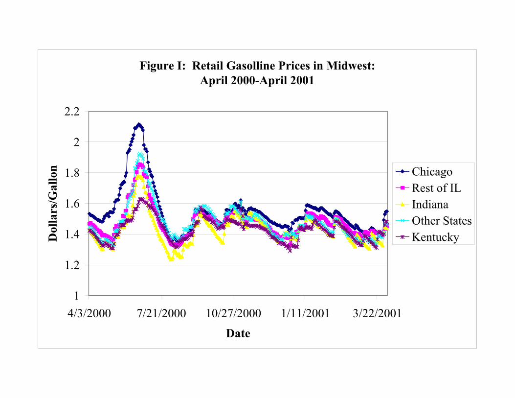
Figure I: Retail Gasolline Prices in Midwest: April 2000-April 2001

1

1.2

1.4

1.6

1.8

2

2.2

4/3/2000 7/21/2000 10/27/2000 1/11/2001 3/22/2001Date

Dol

lars

/Gal

lon Chicago

Rest of ILIndianaOther StatesKentucky

Figure IIC: Winter 2000/2001 Difference in Log Gas Prices IL vs. Neighboring States: MO, IA, WI, IN

0

0.02

0.04

0.06

0.08

1-Dec-00 11-Dec-00 21-Dec-00 31-Dec-00 10-Jan-01 20-Jan-01 30-Jan-01

Date

Log

Poi

nts

Figure IIB: Fall 2000 Difference in Log Gas Prices IN vs. Neighboring States: MI, OH, IL

-0.08

-0.06

-0.04

-0.02

0

0.02

0.04

10/1/2000 10/16/2000 10/31/2000 11/16/2000 11/26/2000

Dates

Log

Poi

nts

Figure IIA: Summer 2000 Difference in Log Gas Prices IL/IN vs. Neighboring States: MI, OH, MO, IA, WI

-0.1

-0.08

-0.06

-0.04

-0.02

0

6/1/2000 6/15/2000 6/29/2000 7/13/2000 7/27/2000

Date

Log

Poi

nts

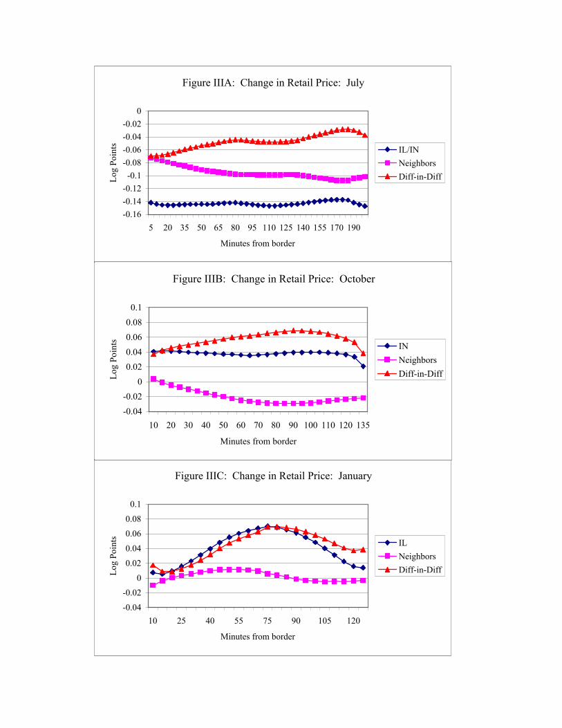
Figure IIIA: Change in Retail Price: July

-0.16-0.14-0.12

-0.1-0.08-0.06-0.04-0.02

0

5 20 35 50 65 80 95 110 125 140 155 170 190

Minutes from border

Log

Poin

ts IL/INNeighborsDiff-in-Diff

Figure IIIC: Change in Retail Price: January

-0.04

-0.020

0.02

0.04

0.060.08

0.1

10 25 40 55 75 90 105 120

Minutes from border

Log

Poin

ts ILNeighborsDiff-in-Diff

Figure IIIB: Change in Retail Price: October

-0.04-0.02

00.020.040.060.08

0.1

10 20 30 40 50 60 70 80 90 100 110 120 135

Minutes from border

Log

Poin

ts INNeighborsDiff-in-Diff

Variable Mean Std. Dev. Mean Std. Dev.Prices retail price 1.67 0.12 1.78 0.14

log(retail price) 0.51 0.07 0.57 0.08wholesale price 1.08 0.06 1.12 0.08log(wholesale price) 0.07 0.05 0.11 0.07federal & state excise tax 0.35 0.02 0.39 0.03

ZIP Code population 19221 13312 21121 15005Characteristics area (square miles) 73.78 61.08 69.80 76.16

gas stations 9.76 7.04 9.75 7.21income 41515 9776 43027 12431

Race white 0.89 0.12 0.87 0.18black 0.05 0.10 0.07 0.16Hispanic 0.03 0.03 0.02 0.04

Age age 0-18 0.27 0.03 0.26 0.04age 19-34 0.21 0.06 0.21 0.06age 35-64 0.38 0.04 0.39 0.04age 65+ 0.14 0.04 0.14 0.04

Education less than high school 0.18 0.07 0.16 0.07high school 0.37 0.08 0.35 0.09some college 0.27 0.04 0.28 0.05college 0.19 0.11 0.21 0.12

Commuting drive alone 0.82 0.05 0.82 0.07car pool 0.11 0.03 0.10 0.04public transport 0.01 0.01 0.01 0.03other transport 0.03 0.03 0.03 0.03work at home 0.03 0.01 0.03 0.020-10 minutes 0.23 0.09 0.22 0.1010-20 minutes 0.33 0.10 0.32 0.1020-30 minutes 0.19 0.08 0.20 0.0730-45 minutes 0.15 0.07 0.16 0.0745-60 minutes 0.05 0.03 0.05 0.0460+ minutes 0.05 0.02 0.05 0.03

Neighboring states: MI, OH, MO, IA, WI. Prices observed June 27, June 28, July 5, & July 65945 Illinois observations; 23488 Neighboring State observations.

Illinois & Indiana Neighboring States

Table I: Selected Summary Statistics: July 2000

A: July Tax RepealDependent Variable: Log(Wholesale Price)

(1) (2) (3) (4)Illinois or Indiana -0.048 -0.013 -0.014 -0.035

(0.038) (0.025) (0.021) (0.017)Post July 1 -0.052 0.029 0.025 -0.088

(0.007) (0.013) (0.015) (0.006)(IL or IN)*Post July 1 -0.035 -0.029 -0.029 -0.007

(0.007) (0.008) (0.008) (0.006)Observations 29675 29675 29433 29433R-Squared 0.23 0.60 0.64 0.57Mean of Dep. Var. 0.560 0.560 0.560 0.560

B: October Tax ReinstatementDependent Variable: Log(Wholesale Price)

(1) (2) (3) (4)Indiana -0.056 -0.052 -0.053 -0.015

(0.009) (0.007) (0.007) (0.001)Post Oct. 31 -0.014 -0.008 -0.009 -0.021

(0.006) (0.006) (0.006) (0.001)IN*Post Oct. 31 0.039 0.040 0.040 -0.005

(0.006) (0.007) (0.006) (0.002)Observations 22092 22092 21884 21884R-Squared 0.16 0.18 0.26 0.41Mean of Dep. Var. 0.457 0.457 0.456 0.456

C: January Tax ReinstatementDependent Variable: Log(Wholesale Price)

(1) (2) (3) (4)Illinois 0.019 -0.001 -0.005 0.029

(0.035) (0.024) (0.021) (0.007)Post Jan. 1 -0.000 -0.038 -0.020 0.051

(0.004) (0.004) (0.004) (0.002)IL*Post Jan. 1 0.027 0.036 0.037 -0.014

(0.004) (0.004) (0.004) (0.003)Observations 7090 7090 7071 7071R-Squared 0.04 0.24 0.39 0.41Mean of Dep. Var. 0.303 0.303 0.303 0.303Controls: Wholesale Price No Yes Yes - ZIP Codes Characteristics No No Yes YesPanel A: Prices observed June 27, June 28, July 5, July 6; Panel B: Prices observed Oct. 26, Oct. 27, Oct. 31, Nov. 1Panel C: Prices observed Dec. 29, Dec. 30, Jan. 2, Jan. 3. Standard errors are reported, clustered at the state level.

Log(Retail Price)

Table II: Regression Results

Log(Retail Price)

Log(Retail Price)

Dependent Variable: (1) (2) (3)

Time Period July Repeal Oct. Reinstatement Jan. ReinstatementIL/IN*Post -0.035 0.032 0.028

(0.012) (0.009) (0.006)IL/IN*Post*1(>=30min & <60min) -0.007 0.001 0.009

(0.006) (0.003) (0.004)IL/IN*Post*1(>=60min & <90min) -0.001 0.012 0.053

(0.007) (0.002) (0.009)IL/IN*Post*1(>=90min) 0.011 0.011 -0.012

(0.010) (0.003) (0.004)Observations 29433 21884 7071R-Squared 0.66 0.28 0.42Mean of Dep. Var. 0.560 0.456 0.303Column(1): Neighboring states: MI, OH, MO, IA, WI & Prices observed June 27, June 28, July 5, July 6Column(2): Neighboring states: MI, OH, IL & Prices observed Oct. 26, Oct. 27, Oct. 31, Nov. 1Column(3): Neighboring states: MO, IA, WI, IN & Prices observed Dec. 29, Dec. 30, Jan. 2, Jan. 3.All models include full controls. Standard errors are reported, clustered at the state level.

Table III: Distance to Border

Log(Retail Price)

A: July Tax Repeal (IL/IN Border)Dependent Variable:

(1) (2) (3)Chicago MSA Other Border MSAs <30 Minutes

Illinois or Indiana 0.066 0.028 0.009(0.001) (0.010) (0.016)

Post July 1 -0.027 -0.028 -0.023(0.001) (0.006) (0.009)

(IL or IN)*Post July 1 -0.027 -0.036 -0.056(0.010) (0.008) (0.013)

Observations 4037 2900 1858R-Squared 0.73 0.79 0.80Mean of Dep. Var. 0.640 0.496 0.506

B: October Tax Reinstatement (IN Border)Dependent Variable:

(1) (2) (3)Chicago MSA Other Border MSAs <30 Minutes

Indiana -0.050 -0.049 -0.043(0.007) (0.005) (0.005)

Post Oct. 31 0.023 -0.013 -0.007(0.001) (0.000) (0.007)

IN*Post Oct. 31 0.001 0.042 0.031(0.001) (0.000) (0.008)

Observations 4040 1251 1047R-Squared 0.65 0.45 0.61Mean of Dep. Var. 0.453 0.460 0.449

C: January Tax Reinstatement (IL Border)Dependent Variable:

(1) (2) (3)Chicago MSA Other Border MSAs <30 Minutes

Illinois 0.047 0.037 0.023(0.019) (0.008) (0.010)

Post Jan. 1 0.001 0.019 0.012(0.002) (0.001) (0.003)

IL*Post Jan. 1 0.027 0.015 0.013(0.003) (0.003) (0.003)

Observations 2449 1098 692R-Squared 0.75 0.54 0.63Mean of Dep. Var. 0.394 0.257 0.267

MSA Fixed Effects No Yes NoIL/IN Border ZIP Fixed Effects No No YesPanel A: Neighboring states: MI, OH, MO, IA, WI & Prices observed 6/27, 6/28, 7/5, 7/6Panel B: Neighboring states: MI, OH, IL & Prices observed 10/26, 10/27, 10/31, 11/1Panel C: Neighboring states: MO, IA, WI, IN & Prices observed 12/29, 12/30, 1/2, 1/3Column (3): Stations closest to KY excluded.All models include full controls. Standard errors are reported, clustered at the state level.

Log(Retail Price)

Table IV: Border Fixed Effects

Log(Retail Price)

Log(Retail Price)

Dependent Variable:

A. Interaction with Number of Stations(1) (2) (3) (4) (5) (6)

July Repeal Oct. Reinstatement Jan. Reinstatement July Repeal Oct. Reinstatement Jan. ReinstatementIL/IN*Post*log(Number of Stations) 0.0050 0.0038 -0.0010 .0044 .0031 .0072

(0.0020) (0.0020) (0.0031) (0.0028) (0.0020) (0.0017)Observations 25324 19797 6665 29765 21884 7071R-Squared 0.66 0.26 0.47 0.62 0.28 0.41Mean of Dep. Var. 0.558 0.455 0.302 0.560 0.456 0.303

B. Interaction with Number of Station Quartiles(1) (2) (3) (1) (2) (3)

July Repeal Oct. Reinstatement Jan. Reinstatement July Repeal Oct. Reinstatement Jan. ReinstatementIL/IN*Post -0.032 0.031 0.044 -0.031 0.039 0.039

(0.007) (0.009) (0.003) (0.007) (0.007) (0.004)IL/IN*Post*Number of Stations 2nd Quartile -0.005 0.010 0.015 0.002 -0.002 -0.003

(0.005) (0.006) (0.007) (0.002) (0.003) (0.006)IL/IN*Post*Number of Stations 3nd Quartile 0.003 0.020 0.004 -0.001 0.000 0.017

(0.006) (0.009) (0.014) (0.003) (0.003) (0.002)IL/IN*Post*Number of Stations Top Quartile 0.029 0.032 -0.019 0.003 0.005 -0.006

(0.009) (0.007) (0.006) (0.002) (0.005) (0.006)Observations 25324 19797 6665 29433 21884 7071R-Squared 0.66 0.27 0.50 0.64 0.28 0.41Mean of Dep. Var. 0.558 0.455 0.302 0.560 0.456 0.303Columns (1)-(3): Number of stations are measured in the hundreds, July sample mean: 4.4 std.dev: 5.2Columns (4)-(6): Number of stations July sample mean: 9.8 std.dev: 7.2Column(1): Neighboring states: MI, OH, MO, IA, WI & Prices observed June 27, June 28, July 5, July 6Column(2): Neighboring states: MI, OH, IL & Prices observed Oct. 26, Oct. 27, Oct. 31, Nov. 1Column(3): Neighboring states: MO, IA, WI, IN & Prices observed Dec. 29, Dec. 30, Jan. 2, Jan. 3.All models include full controls. Standard errors are reported, clustered at the state level.

Table V: Pass through & Number of Gas Stations in the same MSA or ZIP Code

MSA Level ZIP code Level

Log(Retail Price)

A: July Tax RepealDependent Variable:

Population-Weighted Station Fixed Effects S.E. Corrected Timeperiod: Include for Spatial Autocorrelation +/- 1 Month Chicago & KY

(1) (2) (3) (4) (5)Illinois or Indiana -0.020 . -0.013 -0.026 -0.002

(0.020) (0.014) (0.028) (0.018)Post July 1 0.025 -0.029 0.029 -0.005 0.025

(0.018) (0.003) (0.010) (0.013) (0.011)(IL or IN)*Post July 1 -0.027 -0.032 -0.029 -0.033 -0.025

(0.008) (0.010) (0.006) (0.009) (0.010)Observations 29433 21454 29675 351112 36689R-Squared 0.68 0.95 0.60 0.75 0.65Mean of Dep. Var. 0.560 0.560 0.560 0.497 0.561

B: October Tax ReinstatementDependent Variable:

Population-Weighted Station Fixed Effects S.E. Corrected Timeperiod: Include for Spatial Autocorrelation +/- 1 Month Chicago & KY

(1) (2) (3) (4) (5)Indiana -0.055 . -0.052 -0.047 -0.042

(0.005) (0.0002) (0.029) (0.014)Post Oct. 31 -0.014 -0.015 -0.008 -0.098 -0.001

(0.005) (0.006) (0.00005) (0.032) (0.009)IN*Post Oct. 31 0.042 0.040 0.040 0.032 0.032

(0.005) (0.007) (0.0002) (0.033) (0.010)Observations 21884 19215 21890 240473 29468R-Squared 0.27 0.86 0.18 0.39 0.23Mean of Dep. Var. 0.456 0.457 0.457 0.412 0.448

C: January Tax ReinstatementDependent Variable:

Population-Weighted Station Fixed Effects S.E. Corrected Timeperiod: Include for Spatial Autocorrelation +/- 1 Month Chicago & KY

(1) (2) (3) (4) (5)Illinois -0.011 . -0.001 -0.016 0.011

(0.021) (0.017) (0.019) (0.021)Post Jan. 1 -0.019 0.002 -0.038 -0.015 -0.020

(0.004) (0.005) (0.007) (0.009) (0.004)IL*Post Jan. 1 0.038 0.034 0.036 0.042 0.033

(0.004) (0.006) (0.006) (0.008) (0.003)Observations 7071 3106 7090 153951 11086R-Squared 0.41 0.96 0.24 0.45 0.55Mean of Dep. Var. 0.303 0.306 0.303 0.344 0.319All Models include full controls, except Column(3), which includes log(wholesale price) only. Column (1) uses ZIP code population to weight observations.Neighboring states: Columns (1) - (4) as in previous tables; Column (5), includes KY for July and November.Column (4): Data observed one month before and one month after tax change and models include quadratic trend terms allowed to vary by comparison group before and after the policy change.Standard errors are reported, clustered at the state level, except Column (3).

Table VI: Specification Checks

Log(Retail Price)

Log(Retail Price)

Log(Retail Price)

Dependent Variable: (1) (2) (3)

Time Period July Repeal Oct. Reinstatement Jan. ReinstatementLocation & Time Illinois or Indiana -0.014 -0.053** -0.005

(0.020) (0.007) (0.021)Post Reform 0.025 -0.009 -0.020**

(0.015) (0.006) (0.004)(IL or IN)*Post Reform -0.029** 0.040** 0.037**

(0.008) (0.006) (0.004)Price log(wholesale price) 0.891** 0.265 0.623**

(0.142) (0.098) (0.099)ZIP Code population -2.33e-07 -9.71e-08 2.26e-08Characteristics (1.99e-07) (2.15e-07) (2.44e-07)

area (square miles) 2.77e-05 6.65e-05 1.04e-05(2.49e-05) (2.29e-05) (5.17e-05)

gas stations -0.0002 -0.0002 -0.001(0.001) (0.0001) (0.0004)

income 8.96e-07* 0.000 6.92e-07(3.14e-07) (0.000) (4.04e-07)

Race black 0.020 -0.004 -0.006 excluded: white (0.025) (0.010) (0.030)

Hispanic 0.088** -0.036* 0.066(0.023) (0.006) (0.081)

Age age 19-34 0.057 0.003 -0.005excluded: age 0-18 (0.041) (0.022) (0.095)

age 35-64 0.124 0.041 0.100(0.056) (0.042) (0.060)

age 65+ 0.088 -0.050 -0.116(0.045) (0.031) (0.116)

Education high school 0.057 -0.004 0.386* excluded: HS drop out (0.145) (0.064) (0.109)

some college 0.116 0.009 0.191(0.068) (0.032) (0.162)

college -0.002 0.046 0.208*Commuting (0.070) (0.038) (0.061) excluded: drive alone, car pool 0.087* 0.114** 0.154 work at home (0.028) (0.016) (0.062) and 0-10 minutes public transport 0.251 0.046 0.305

(0.130) (0.112) (0.212)other transport 0.168 0.070 0.249

(0.071) (0.052) (0.103)10-20 minutes -0.092 -0.010 -0.124

(0.041) (0.031) (0.044)20-30 minutes -0.088* 0.003 -0.082

(0.030) (0.035) (0.046)30-45 minutes -0.103 0.012 -0.226*

(0.066) (0.019) (0.072)45-60 minutes -0.141 0.005 -0.281

(0.064) (0.051) (0.113)60+ minutes -0.057 0.047 -0.020

(0.077) (0.051) (0.081)Observations 29433 21884 7071R-Squared 0.64 0.26 0.39Mean of Dep. Var. 0.560 0.456 0.303

Column (1): Prices observed June 27, June 28, July 5, July 6; Column (2): Prices observed Oct. 27, Oct. 31, Nov. 1, Nov. 2;Column (3): Prices observed Dec. 29, Dec. 30, Jan. 2, Jan. 3. Standard errors are reported, clustered at the state level.Models also include indicators for major brands. *=significant at 5%, **=significant at 1%.

Log(Retail Price)

Table A1: Full Regression Results

A: July Tax RepealDependent Variable:

(1) (2) (3)Time Period July Repeal Nov. Re-Instatement Jan. Re-Instatement

IL/IN*1(t-10) 0.009 -0.000 0.025(0.031) (0.016) (0.010)

IL/IN*1(t-9) 0.012 0.002 0.020(0.032) (0.008) (0.013)

IL/IN*1(t-8) 0.013 0.002 0.005(0.030) (0.009) (0.009)

IL/IN*1(t-7) 0.003 -0.000 -0.000(0.025) (0.009) (0.008)

IL/IN*1(t-6) 0.002 0.000 0.003(0.025) (0.010) (0.007)

IL/IN*1(t-5) 0.006 0.003 0.006(0.020) (0.010) (0.007)

IL/IN*1(t-4) 0.002 -0.003 0.004(0.016) (0.002) (0.007)

IL/IN*1(t-3) 0.003 0.001 0.007(0.012) (0.003) (0.006)

IL/IN*1(t-2) 0.007 -0.002 0.009(0.008) (0.002) (0.006)

IL/IN*Post -0.022** 0.037** 0.046**(0.004) (0.005) (0.007)

IL/IN*1(t+2) -0.008 0.006 -0.001(0.003) (0.002) (0.006)

IL/IN*1(t+3) -0.003 0.006 -0.016(0.005) (0.003) (0.012)

IL/IN*1(t+4) -0.005 0.001 -0.016(0.005) (0.006) (0.018)

IL/IN*1(t+5) 0.007 0.003 -0.020(0.007) (0.007) (0.014)

IL/IN*1(t+6) 0.002 -0.005 -0.019(0.008) (0.012) (0.012)

IL/IN*1(t+7) 0.003 -0.000 -0.022*(0.009) (0.014) (0.008)

IL/IN*1(t+8) 0.006 0.010* -0.030**(0.009) (0.003) (0.002)

IL/IN*1(t+9) 0.005 -0.032** -0.025**(0.012) (0.003) (0.002)

IL/IN*1(t+10) 0.005 -0.033** -0.032*(0.011) (0.002) (0.010)

Observations 168942 113678 47688R-Squared 0.75 0.37 0.46Mean of Dep. Var. 0.544 0.432 0.320Omitted category is the day before the reform and the post reform coefficients represent the difference from the day after the reform.Column(1): Neighboring states: MI, OH, MO, IA, WI Prices observed 6/14,6/15,6/16,6/19,6/20,6/21,6/22,6/23,6/27,6/28,7/5,7/6,7/7,7/8,7/11,7/12,7/13,7/14,7/15,7/18

Prices observed 10/16,10/17,10/18,10/19,10/20,10/23,10/24,10/25,10/26,10/27,10/31,11/1,11/2,11/3,11/6,11/7,11/10,11/13,11/14,11/15Column(3): Neighboring states: MO, IA, WI, IN & Prices observed Dec. 29, Dec. 30, Jan. 2, Jan. 3. Prices observed 12/19,12/20,12/21,12/22,12/23,12/24,12/25,12/26,12/29,12/30,1/2,1/3,1/4,1/5,1/6,1/7,1/8,1/9,1/10,1/11All models include full controls including main effects of the time indicators. Standard errors are reported, clustered at the state level. *=significant at 5%, **=significant at 1%.

Table A2: Expaned Timeframe

Log(Retail Price)

Column(2): Neighboring states: MI, OH, IL & Prices observed Oct. 27, Oct. 31, Nov. 1, Nov. 2

ID

AZ

UT

MT

WY

NM

CO

AL

FL

SC

TN

KY

INOH

NC

SD

KS

NE

MN

WI

IA

IL

MO

AR

MS

OK

ND

OR

CA NV

WA

TX

MI

PA

ME

VA

NY

CT

WV

MD

NJ

VTNH

MA

DE

RI

Figure A1: Selected Midwest States

LA

GA

Buy SmartDraw!- purchased copies print this document without a watermark .

Visit www.smartdraw.com or call 1-800-768-3729.