Navigation System for a Mobile Robot

Based on Omni-directional Vision

Jan Benda, Jan Flusser

jan.benda@matfyz.czflusser@utia.cas.cz

Institute of Information Theory and Automation,

Academy of Sciences of the Czech Republic

Prague, January 2006

Acknowledgement:This work was supported by the project No. 1M0572 (Research Center DAR)of the Czech Ministry of Education

Abstract:

The work addresses the vast problem of mobile robot localization in thedynamic environment of a robotic contest. A method based on particle filtersusing only the image of a catadioptric visual sensor as its input is developed.The advantage of this approach is increased robustness to external influencessuch as robot collisions and easy portability thanks to independence on othersystems of the mobile robot. The proposed method employs a compositionof fast color thresholding, look-up coordinate transform, vision-based motionprediction and Monte Carlo Localization to gain robust and reliable posetracking using a color map of a delimited environment. Since the system usesvisual data both to determine the relative motion and to verify the currentlocation, it can cope well with unexpected events such as wheel slippage orcollision.

Keywords: mobile robot, localization, real-time tracking, omni-directionalvision

3

Contents

1 Introduction 81.1 Preface . . . . . . . . . . . . . . . . . . . . . . . . . . . . . . . 8

2 Problem Analysis 102.1 Architectures . . . . . . . . . . . . . . . . . . . . . . . . . . . 10

2.1.1 Behavioral . . . . . . . . . . . . . . . . . . . . . . . . . 102.1.2 Deliberative . . . . . . . . . . . . . . . . . . . . . . . . 11

2.2 Sensors . . . . . . . . . . . . . . . . . . . . . . . . . . . . . . . 132.2.1 Range-finders . . . . . . . . . . . . . . . . . . . . . . . 132.2.2 Beacons . . . . . . . . . . . . . . . . . . . . . . . . . . 152.2.3 Vision . . . . . . . . . . . . . . . . . . . . . . . . . . . 162.2.4 Omni-directional Vision . . . . . . . . . . . . . . . . . 17

2.3 Approaches . . . . . . . . . . . . . . . . . . . . . . . . . . . . 182.3.1 Global Localization vs. Tracking . . . . . . . . . . . . 192.3.2 Geometrical vs. Topological Approach . . . . . . . . . 202.3.3 Probabilistic vs. Analytical Approach . . . . . . . . . . 202.3.4 Feature-Based vs. Image-Based Evaluation . . . . . . . 232.3.5 Natural and Artificial Landmarks . . . . . . . . . . . . 24

2.4 Related Work . . . . . . . . . . . . . . . . . . . . . . . . . . . 252.4.1 Appearance-Based Approach . . . . . . . . . . . . . . . 252.4.2 Feature-Based Approach . . . . . . . . . . . . . . . . . 292.4.3 Contest Environment . . . . . . . . . . . . . . . . . . . 31

2.5 Proposed Solution . . . . . . . . . . . . . . . . . . . . . . . . . 362.5.1 Target Environment . . . . . . . . . . . . . . . . . . . 362.5.2 Task Formulation . . . . . . . . . . . . . . . . . . . . . 372.5.3 Selected Approach . . . . . . . . . . . . . . . . . . . . 38

3 Theory 403.1 Omni-directional Vision . . . . . . . . . . . . . . . . . . . . . 403.2 Color perception . . . . . . . . . . . . . . . . . . . . . . . . . 423.3 Monte Carlo Localization . . . . . . . . . . . . . . . . . . . . . 44

4

3.3.1 Prediction . . . . . . . . . . . . . . . . . . . . . . . . . 443.3.2 Update . . . . . . . . . . . . . . . . . . . . . . . . . . . 45

4 Implementation 474.1 Filters and Chains . . . . . . . . . . . . . . . . . . . . . . . . 474.2 Pre-processing . . . . . . . . . . . . . . . . . . . . . . . . . . . 48

4.2.1 Input Enhancement . . . . . . . . . . . . . . . . . . . . 484.2.2 Color Classification . . . . . . . . . . . . . . . . . . . . 494.2.3 Color Display . . . . . . . . . . . . . . . . . . . . . . . 504.2.4 Image Rectification . . . . . . . . . . . . . . . . . . . . 50

4.3 Prediction . . . . . . . . . . . . . . . . . . . . . . . . . . . . . 514.4 Correction . . . . . . . . . . . . . . . . . . . . . . . . . . . . . 53

5 Experiments 565.1 Simulated Environment . . . . . . . . . . . . . . . . . . . . . . 565.2 Target Environment . . . . . . . . . . . . . . . . . . . . . . . 58

6 Conclusion 636.1 Results . . . . . . . . . . . . . . . . . . . . . . . . . . . . . . . 636.2 Future Research . . . . . . . . . . . . . . . . . . . . . . . . . . 64

Appendices 65

A Eurobotopen 2005 65A.1 Rules . . . . . . . . . . . . . . . . . . . . . . . . . . . . . . . . 65A.2 Playing Field . . . . . . . . . . . . . . . . . . . . . . . . . . . 65

B Target Robotic Platform 68

C Attachment CD Contents 70

D Software Documentation 72D.1 Vision Framework Usage . . . . . . . . . . . . . . . . . . . . . 72D.2 Description of Vision Framework Files . . . . . . . . . . . . . 74

5

List of Figures

2.1 Overview of the general control architectures . . . . . . . . . . 112.2 Overview of the sensor modalities used in mobile robot local-

ization . . . . . . . . . . . . . . . . . . . . . . . . . . . . . . . 132.3 The time-of-flight Swiss Ranger sensor . . . . . . . . . . . . . 142.4 Omni-directional vision used as an affordable range-finder re-

placement . . . . . . . . . . . . . . . . . . . . . . . . . . . . . 172.5 Classification of omni-vision based approaches . . . . . . . . . 192.6 Power spectrum of the Fourier transform of cylindrical projec-

tion of an omni-directional image . . . . . . . . . . . . . . . . 262.7 Eigenvector images computed for a database of rotated images 272.8 Important edges in an omni-directional image and the respec-

tive distance transform . . . . . . . . . . . . . . . . . . . . . . 282.9 Minimum free space estimation . . . . . . . . . . . . . . . . . 292.10 A light map of a museum ceiling . . . . . . . . . . . . . . . . . 302.11 Feature-based matching against the image database . . . . . . 312.12 Bird’s eye view of the RoboCup field . . . . . . . . . . . . . . 322.13 The process of estimating playing field position . . . . . . . . 332.14 Possible locations of a robot observing a relative bearing of

two landmarks . . . . . . . . . . . . . . . . . . . . . . . . . . . 342.15 Searching for geometrical features in an omni-directional image 342.16 Visual range-finder measurements from an omni-directional

image . . . . . . . . . . . . . . . . . . . . . . . . . . . . . . . 352.17 Playing field for the Eurobotopen 2005 contest . . . . . . . . . 372.18 Overview of the vision-based localization process . . . . . . . . 38

3.1 Examples of Non-SVP and SVP projections . . . . . . . . . . 413.2 Schematic for the ground plane projection and rectification . . 423.3 Representation of landmark color classes in the YCrCb space . 43

4.1 NormYUVFilter overview . . . . . . . . . . . . . . . . . . . . . 484.2 ThreshBoundFilter overview . . . . . . . . . . . . . . . . . . 494.3 ColorFilter overview . . . . . . . . . . . . . . . . . . . . . . 50

6

4.4 ProjectFilter overview . . . . . . . . . . . . . . . . . . . . . 514.5 ProjectFilter overview . . . . . . . . . . . . . . . . . . . . . 524.6 SumFilter overview . . . . . . . . . . . . . . . . . . . . . . . 524.7 VisualMclFilter overview . . . . . . . . . . . . . . . . . . . 544.8 Likelihood plot for different robot positions given the actual

observations . . . . . . . . . . . . . . . . . . . . . . . . . . . . 55

5.1 Simulated tracking experiment . . . . . . . . . . . . . . . . . . 575.2 Average displacement error in the simulation experiment with

respect to the particle count . . . . . . . . . . . . . . . . . . . 575.3 Real-world tracking experiment . . . . . . . . . . . . . . . . . 595.4 The trajectories estimated using the vision-based method ren-

dered for the eight test video streams . . . . . . . . . . . . . . 595.5 Influence of particle count on accuracy of rotation tracking . . 605.6 Influence of particle count on the probability of successful pose

tracking . . . . . . . . . . . . . . . . . . . . . . . . . . . . . . 61

A.1 The plan of the Eurobotopen 2005 contest playing field . . . . . 66

B.1 The test robotic platform with the omni-directional sensormounted on top . . . . . . . . . . . . . . . . . . . . . . . . . . 69

7

Chapter 1

Introduction

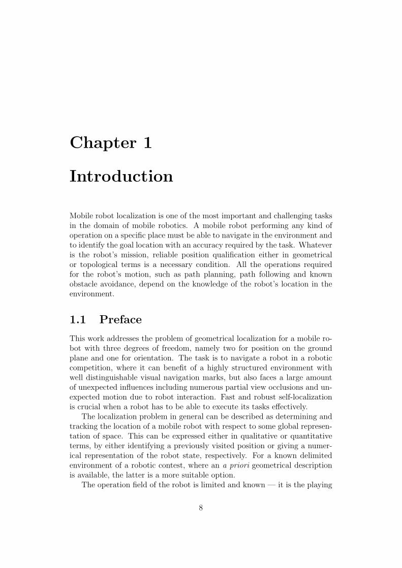
Mobile robot localization is one of the most important and challenging tasksin the domain of mobile robotics. A mobile robot performing any kind ofoperation on a specific place must be able to navigate in the environment andto identify the goal location with an accuracy required by the task. Whateveris the robot’s mission, reliable position qualification either in geometricalor topological terms is a necessary condition. All the operations requiredfor the robot’s motion, such as path planning, path following and knownobstacle avoidance, depend on the knowledge of the robot’s location in theenvironment.

1.1 Preface

This work addresses the problem of geometrical localization for a mobile ro-bot with three degrees of freedom, namely two for position on the groundplane and one for orientation. The task is to navigate a robot in a roboticcompetition, where it can benefit of a highly structured environment withwell distinguishable visual navigation marks, but also faces a large amountof unexpected influences including numerous partial view occlusions and un-expected motion due to robot interaction. Fast and robust self-localizationis crucial when a robot has to be able to execute its tasks effectively.

The localization problem in general can be described as determining andtracking the location of a mobile robot with respect to some global represen-tation of space. This can be expressed either in qualitative or quantitativeterms, by either identifying a previously visited position or giving a numer-ical representation of the robot state, respectively. For a known delimitedenvironment of a robotic contest, where an a priori geometrical descriptionis available, the latter is a more suitable option.

The operation field of the robot is limited and known — it is the playing

8

field of the Eurobotopen 2005 robotic contest. Although the prototype solutiontargets this specific environment, the proposed approach and the developedalgorithms can be reused in different contest environments.

The presented work is divided into four chapters. Chapter 2 presentsand further specifies the given task seeking for an optimal strategy. Sev-eral possibilities of non-visual and visual methods applicable for the targetenvironment are discussed highlighting probabilistic approaches. The choiceof omni-directional imaging is substantiated, examples of known applicationsare given, and a customized solution is presented. In Chapter 3, a theoreticalbackground for omni-directional image formation, color perception and par-ticle filtering is given. Chapter 4 describes the prototype implementation indetail. The experiments in Chapter 5 display the performance of the selectedapproach and describe the limits of the method and the problems open forfuture research.

9

Chapter 2

Problem Analysis

Ongoing research on mobile robotics provides numerous approaches to thelocalization problem. The selection of an appropriate method is a key task onthe way to successful implementation. The following subsections will discussthe derivation of the proposed solution.

2.1 Architectures

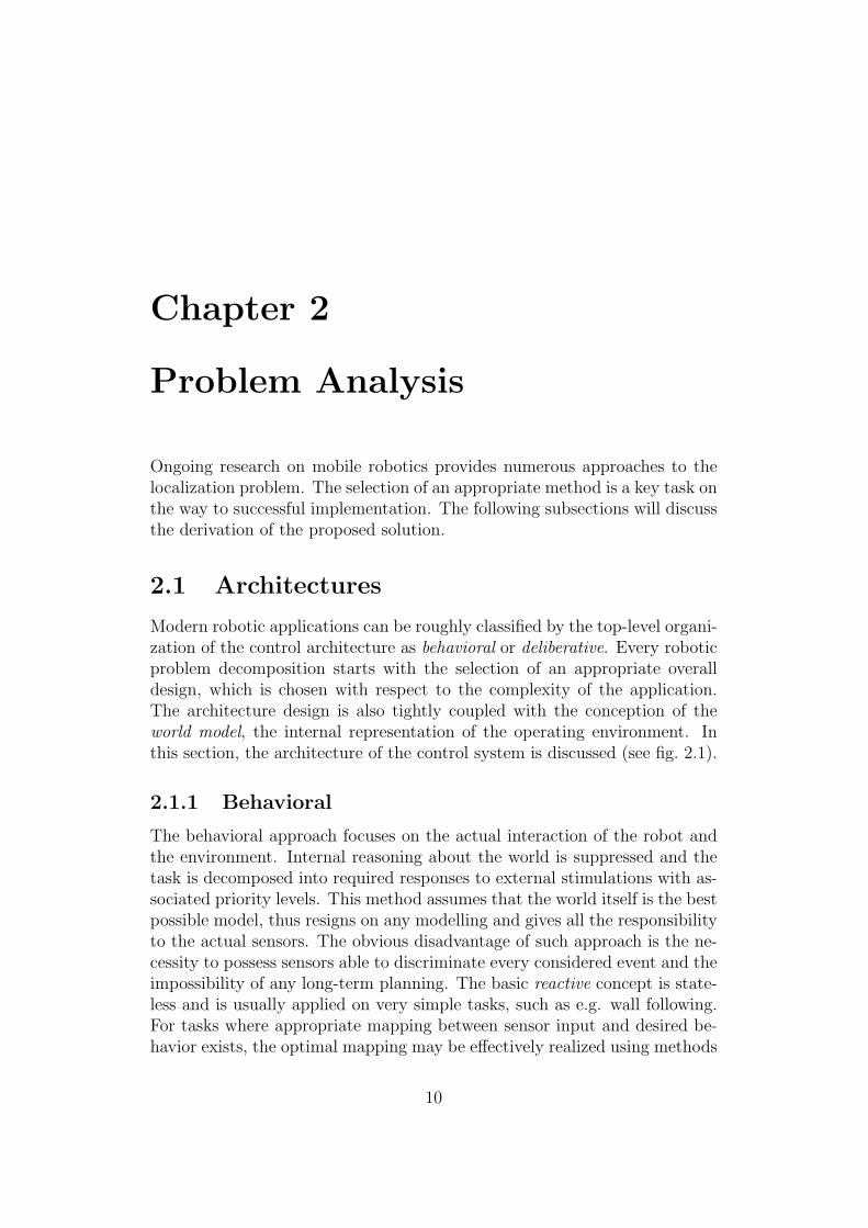
Modern robotic applications can be roughly classified by the top-level organi-zation of the control architecture as behavioral or deliberative. Every roboticproblem decomposition starts with the selection of an appropriate overalldesign, which is chosen with respect to the complexity of the application.The architecture design is also tightly coupled with the conception of theworld model, the internal representation of the operating environment. Inthis section, the architecture of the control system is discussed (see fig. 2.1).

2.1.1 Behavioral

The behavioral approach focuses on the actual interaction of the robot andthe environment. Internal reasoning about the world is suppressed and thetask is decomposed into required responses to external stimulations with as-sociated priority levels. This method assumes that the world itself is the bestpossible model, thus resigns on any modelling and gives all the responsibilityto the actual sensors. The obvious disadvantage of such approach is the ne-cessity to possess sensors able to discriminate every considered event and theimpossibility of any long-term planning. The basic reactive concept is state-less and is usually applied on very simple tasks, such as e.g. wall following.For tasks where appropriate mapping between sensor input and desired be-havior exists, the optimal mapping may be effectively realized using methods

10

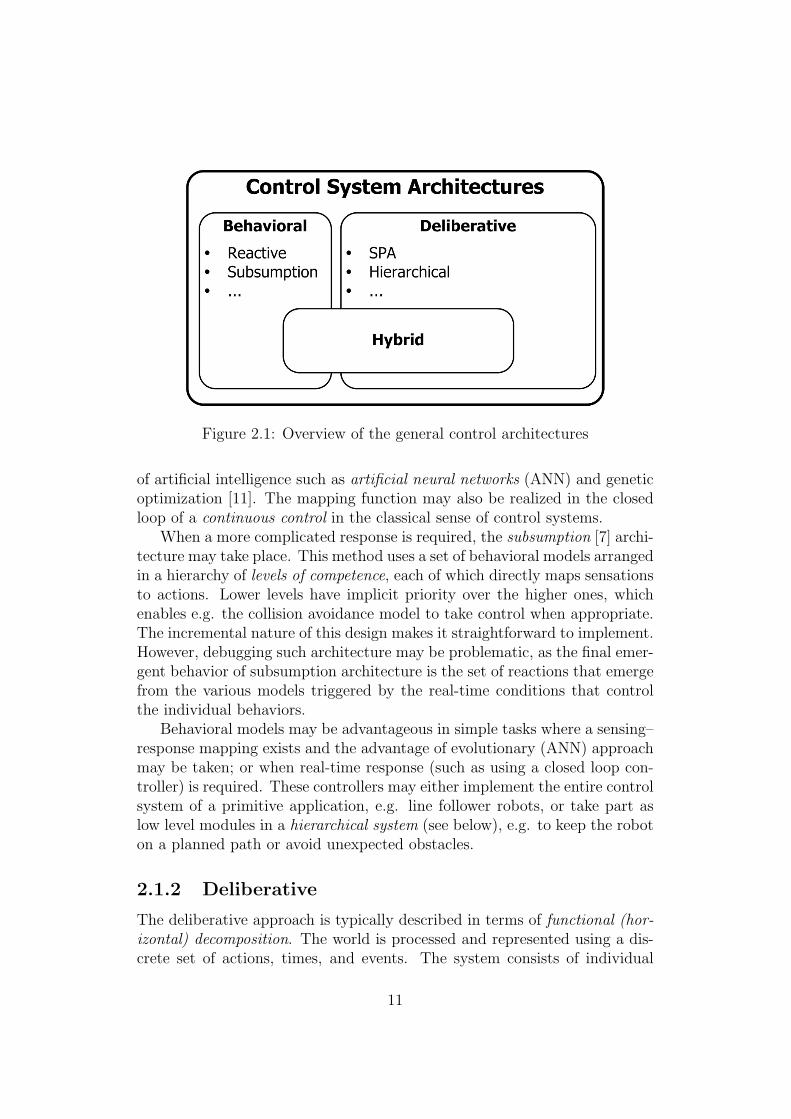
Figure 2.1: Overview of the general control architectures

of artificial intelligence such as artificial neural networks (ANN) and geneticoptimization [11]. The mapping function may also be realized in the closedloop of a continuous control in the classical sense of control systems.

When a more complicated response is required, the subsumption [7] archi-tecture may take place. This method uses a set of behavioral models arrangedin a hierarchy of levels of competence, each of which directly maps sensationsto actions. Lower levels have implicit priority over the higher ones, whichenables e.g. the collision avoidance model to take control when appropriate.The incremental nature of this design makes it straightforward to implement.However, debugging such architecture may be problematic, as the final emer-gent behavior of subsumption architecture is the set of reactions that emergefrom the various models triggered by the real-time conditions that controlthe individual behaviors.

Behavioral models may be advantageous in simple tasks where a sensing–response mapping exists and the advantage of evolutionary (ANN) approachmay be taken; or when real-time response (such as using a closed loop con-troller) is required. These controllers may either implement the entire controlsystem of a primitive application, e.g. line follower robots, or take part aslow level modules in a hierarchical system (see below), e.g. to keep the roboton a planned path or avoid unexpected obstacles.

2.1.2 Deliberative

The deliberative approach is typically described in terms of functional (hor-izontal) decomposition. The world is processed and represented using a dis-crete set of actions, times, and events. The system consists of individual

11

modules operating in a deterministic serial fashion. In this architecture,commonly known as Sense-Plan-Act (SPA), the robot periodically executesa series of ’percept-model-plan-execute’ modules with the output of onemodule being input of the following. Although it is hard to reach real-timeresponse of such system, functional examples exist [35].

To be able to both perform in real time and allow for complex modelmanipulation and reasoning, the system must be designed as hierarchical [11].A typical design would include a persistent world model, which is periodicallyupdated with the sensed data and used for reasoning. The individual modulesin the hierarchical model are all required to have real-time response, i.e.to finish every execution cycle in a fixed period of time. In contrast withthe classical SPA, these modules typically run concurrently, which allowsdifferent update rates of individual modules. This approach is well suitedfor vision-based navigation and reasoning that typically requires significanttime for processing one captured image. Although this time may be keptconstant, it will typically be much longer than the execution time of e.g. alow-level motion controller.

In a strict hierarchical system, the high-level layers such as mission plan-ning and operational activity monitoring have full control over the layersthat provide low-level control of the robot’s sensors and actuators. Thisalso defines the mechanism for propagation of information and control se-quences. In a blackboard system [11], the communication between modulesis provided by a neutral common information pool, shared by the individualcomputational processes. Fundamental to any blackboard-based system isa mechanism to provide efficient communication between the various com-putational agents and the blackboard. A mechanism that proves elegant,effective, and scalable is the publish-subscribe model. In this scenario, theactual world model variables reside in the individual agents providing theremaining modules with access to the contained variables using a commoncommunication system. The common pool thus serves only for pairing thepublishers containing the variables with the subscribers requesting access tothe data. The key task is to distribute the world model so that inter-modulecommunication is minimized.

Note that the global conception of the target control architecture falls be-yond the scope of this work and is not described here. The work focuses onone fundamental part of the complex system, which is the localization mod-ule. The other essential components, such as the motion control and planningalgorithms are not covered. The modular approach enables to design the indi-vidual components in an isolated manner. The localization module processesthe output of sensoric subsystems and produces the position information viaa defined interface.

12

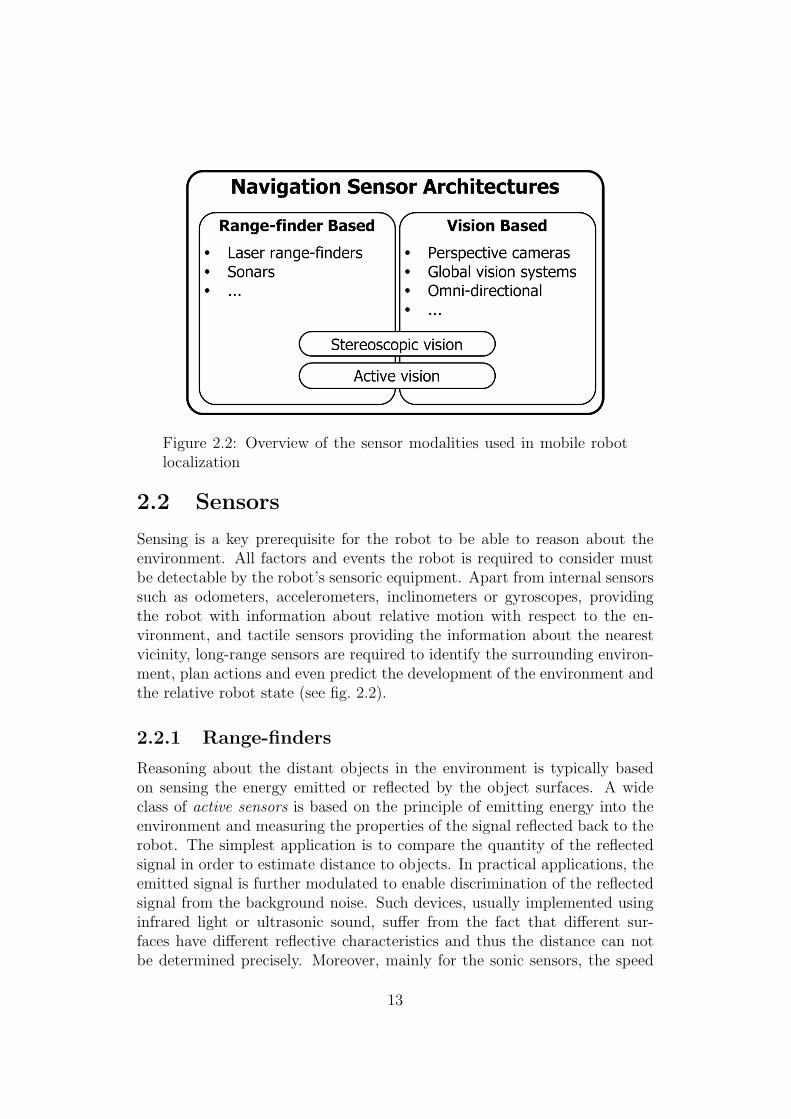
Figure 2.2: Overview of the sensor modalities used in mobile robotlocalization

2.2 Sensors

Sensing is a key prerequisite for the robot to be able to reason about theenvironment. All factors and events the robot is required to consider mustbe detectable by the robot’s sensoric equipment. Apart from internal sensorssuch as odometers, accelerometers, inclinometers or gyroscopes, providingthe robot with information about relative motion with respect to the en-vironment, and tactile sensors providing the information about the nearestvicinity, long-range sensors are required to identify the surrounding environ-ment, plan actions and even predict the development of the environment andthe relative robot state (see fig. 2.2).

2.2.1 Range-finders

Reasoning about the distant objects in the environment is typically basedon sensing the energy emitted or reflected by the object surfaces. A wideclass of active sensors is based on the principle of emitting energy into theenvironment and measuring the properties of the signal reflected back to therobot. The simplest application is to compare the quantity of the reflectedsignal in order to estimate distance to objects. In practical applications, theemitted signal is further modulated to enable discrimination of the reflectedsignal from the background noise. Such devices, usually implemented usinginfrared light or ultrasonic sound, suffer from the fact that different sur-faces have different reflective characteristics and thus the distance can notbe determined precisely. Moreover, mainly for the sonic sensors, the speed

13

Figure 2.3: The time-of-flight Swiss Ranger sensor that is able toprovide real-time depth maps of the environment, reprinted from [50]

of distribution of the signal through the environment depends on environ-mental properties such as temperature and humidity. These simple sensorsare thus often used as proximity detectors, kind of early-warning bumpers.More advanced approach considers additional features of the reflected signal,such as reflection angle for triangulation [4] or time-of-flight [11].

Using electromagnetic waves in conjunction with time-of-flight or phase-based measurements is a very robust and reliable technique. Both methodsuse the time delay of signal propagation. This is especially advantageous con-sidering the high and relatively invariable speed of light. On the other hand,it poses significant requirements on signal processing, making such devicesrelatively expensive. Various applications exist, exploiting the characteris-tics of specific wavelengths, from long-range radars to high precision laserrange-finders (LRF). These devices are usually able to take very frequentdistance measurements along a defined ray. Therefore it is possible to ex-tend the measurement to multiple directions by reflecting the measurementray [1]. As mobile robots usually operate on a flat surface, one range-finderscanning a single horizontal plane is sufficient for navigation tasks. Someobstacles, however, such as furniture or steps require scanning in additionalplanes. More range-finders may be added or a single device may be pointedto different directions to get better coverage of the space in front of the ro-bot. Advanced sensors providing direct real-time 3D imaging also exist (seefig. 2.3).

For modern robotic applications, the laser or sonar range-finders are verypopular, although these sensors have a number of problems. They tend to beeasily confused in highly dynamic environments, e.g. when the laser or sonarbeams are blocked by people or other robots. The operation area must alsobe populated with objects detectable by the range-finders. The localizationprocess using range-finder measurements requires that the operation field issurrounded by walls. Unfortunately, this is not the case for many roboticcontests, as the operation fields for the contests are flat and may be placed

14

in an arbitrary indoor area. Localization in such environments using LRFsis feasible, but is far from being simple and inexpensive [20].

Additionally, feature estimates obtained from rangefinder measurementsare generic, without any uniquely defining characteristics. This poses a dif-ficult problem for solving the data association problem between the currentmeasurements and the map, where a single feature observation might requirecomparison with the entire map. This is an important drawback comparingto vision-based sensors, which usually provide a great deal of contextual in-formation that can constrain data association, and reduce the cost of featurematching [45].

2.2.2 Beacons

A tempting approach is to use a navigation system based on bearing or dis-tance measurements towards a set of beacons — active devices whose locationis known. A popular example is the Global Positioning System (GPS). A GPSreceiver can be localized with the accuracy of tens of meters anywhere onthe globe using 21 Earth-orbiting satellites. The accuracy may be furtherincreased using Differential GPS (DGPS) systems, where a reference GPSreceiver with known coordinates transmits the current relative error of theGPS system, although the gain in accuracy is negligible after the selectiveavailability encryption for civilian receivers was removed [37]. A still moreaccurate form of DGPS called Differential Carrier GPS exists. This systemuses the difference in carrier cycle measurements between the mobile andthe reference receivers and can achieve accuracy of centimeters. Naturally,Differential Carrier GPS is substantially more costly than basic DGPS [11].One of the great advantages of the GPS system is that is does not involveany other observation of the external environment. It is also a purely passivesystem that involves no energy output by the receiver, which makes it idealfor military applications. Unfortunately, for majority of robotic applications,the tradeoff between price and accuracy is unreachable. Moreover, for indoormobile robots reliable GPS signal coverage is often missing.

Another possibility is to create a special beacon system customized forthe indoor navigation task. It would even be applicable to a contest environ-ment where several active or passive landmarks may be installed in knownpositions. Many possibilities exist, e.g. triangulation using time-of-flightmeasured distances of beacons emitting ultrasonic pulses or using relativebearing measurements towards light-reflecting landmarks. Unfortunately,such system would require expensive custom electro-mechanical design andmanufacturing, which makes it unavailable for the considered application.

15

2.2.3 Vision

As described so far, the entire class of active sensors is not appropriate forthe target environment. Rejecting the active emission of energy by the robotitself as well as by external beacons, one important class of sensors remains— the visual perception. Providing the robot with the ability to ”see”, i.e.process and interpret 2D images of the environment acquired by a camera,has many advantages as well as drawbacks. A positive aspect is that human-populated environments are vision-friendly as vision is the dominant senseused by people. Even in unmodified environments, the important featuresrelevant to navigation, such as steps or door-posts, are made visually dis-criminable.

The major drawback and most significant challenge of a general computervision task is the ambiguity of inverse mapping from the 2D perspective pro-jection back into the 3D space. The most general approach, inspired by thehuman stereoscopic vision, employs two or more cameras and the relative shiftof correspondent features to determine their distance from the observer. Ac-tive vision methods combining the active and passive approaches are some-times used in scene reconstruction — a known pattern projected onto theobserved scene helps to disambiguate the inverse perspective projection. Forexample the light striping technique, which uses a laser beam to highlighta plane, whose intersection with the surrounding objects is triangulated toobtain the depth estimation [11]. To avoid the computationally demandingscene reconstruction, constraints may be applied on the locations of the ob-served features, e.g. positioning them all on a single plane. The perspectiveprojection of this subset of features then becomes a bijection. Concerning acontest environment, the distinctive markers on the floor represent exactlythis class of features.

An important factor that led to the selection of visual approach for thegiven environment is that the operation field contains well structured land-marks discriminable by color. Moreover, due to their small vertical diversity,a minimal error is introduced assuming their location is on the ground-plane.Based on this assumption, the environment can be represented using a 2Dmap of ground color and the scene reconstruction may be simplified to aone-to-one function. Camera is also a perfect sensor for tracking proximatecolor landmarks as it provides high amount of data for a relatively low cost.On the other hand, a computationally efficient approach to the extractionof landmark information is difficult to implement. Appropriate choice of thevisual sensor configuration may help to ease the task.

16

Figure 2.4: Omni-directional vision can be used as an afford-able range-finder replacement. Here, distances to different visuallandmarks determined by color transition are measured, reprintedfrom [32]

2.2.4 Omni-directional Vision

The feature that makes traditional perspective cameras hardly applicable torobot localization is the limited field of view and the emerging viewpointand occlusion problems. A single camera may be occluded by an obstacleor the robot may be facing a direction where no appropriate landmarks areobservable [47]. When the operation field is small, an overhead camera maybe mounted monitoring the entire area, such as for example in the RoboCupSmall Size League competition. Unfortunately, no suitable location for aglobal vision camera exists in the target environment.

To address the field-of-view problem, multiple-camera solutions, activepanning, or fish-eye lenses have been proposed. An alternative is to usespecially designed mirrors to bring a larger portion of the environment intothe field of view of the camera (see fig. 2.4). Such configurations are calledcatadioptric as they employ both reflection and refraction in the process ofimage formation. The camera is typically mounted in the upwards directionwith the mirror above it providing the robot with a 360◦ view of the environ-ment [11]. Panoramic or omni-directional cameras have become popular forself-localization in recent years because of their relatively low cost and largefield of view, which makes it possible to define features that are invariant tothe robot’s orientation [3].

One of the objectionable features of panoramic sensors is the relatively lowspatial resolution. For applications that require both wide field of view and

17

high resolution, a high-resolution camera [9] or multi-camera solution [23]may be applied. However, for the majority of applications the resolutionof a general camera is sufficient, besides the fact that a higher amount ofdata could be too complicated to process. Equipping the robot with anadditional perspective camera providing detailed view of one particular areaof interest [18] is a suitable compromise in many cases.

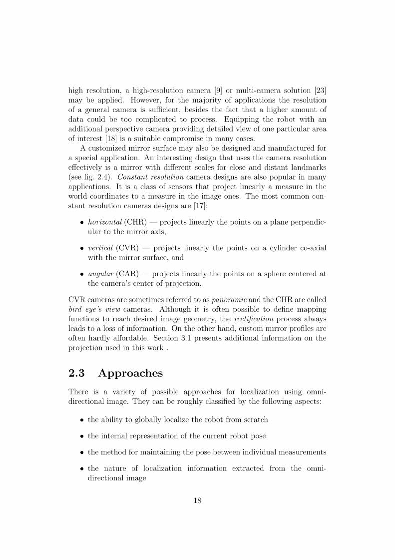
A customized mirror surface may also be designed and manufactured fora special application. An interesting design that uses the camera resolutioneffectively is a mirror with different scales for close and distant landmarks(see fig. 2.4). Constant resolution camera designs are also popular in manyapplications. It is a class of sensors that project linearly a measure in theworld coordinates to a measure in the image ones. The most common con-stant resolution cameras designs are [17]:

• horizontal (CHR) — projects linearly the points on a plane perpendic-ular to the mirror axis,

• vertical (CVR) — projects linearly the points on a cylinder co-axialwith the mirror surface, and

• angular (CAR) — projects linearly the points on a sphere centered atthe camera’s center of projection.

CVR cameras are sometimes referred to as panoramic and the CHR are calledbird eye’s view cameras. Although it is often possible to define mappingfunctions to reach desired image geometry, the rectification process alwaysleads to a loss of information. On the other hand, custom mirror profiles areoften hardly affordable. Section 3.1 presents additional information on theprojection used in this work .

2.3 Approaches

There is a variety of possible approaches for localization using omni-directional image. They can be roughly classified by the following aspects:

• the ability to globally localize the robot from scratch

• the internal representation of the current robot pose

• the method for maintaining the pose between individual measurements

• the nature of localization information extracted from the omni-directional image

18

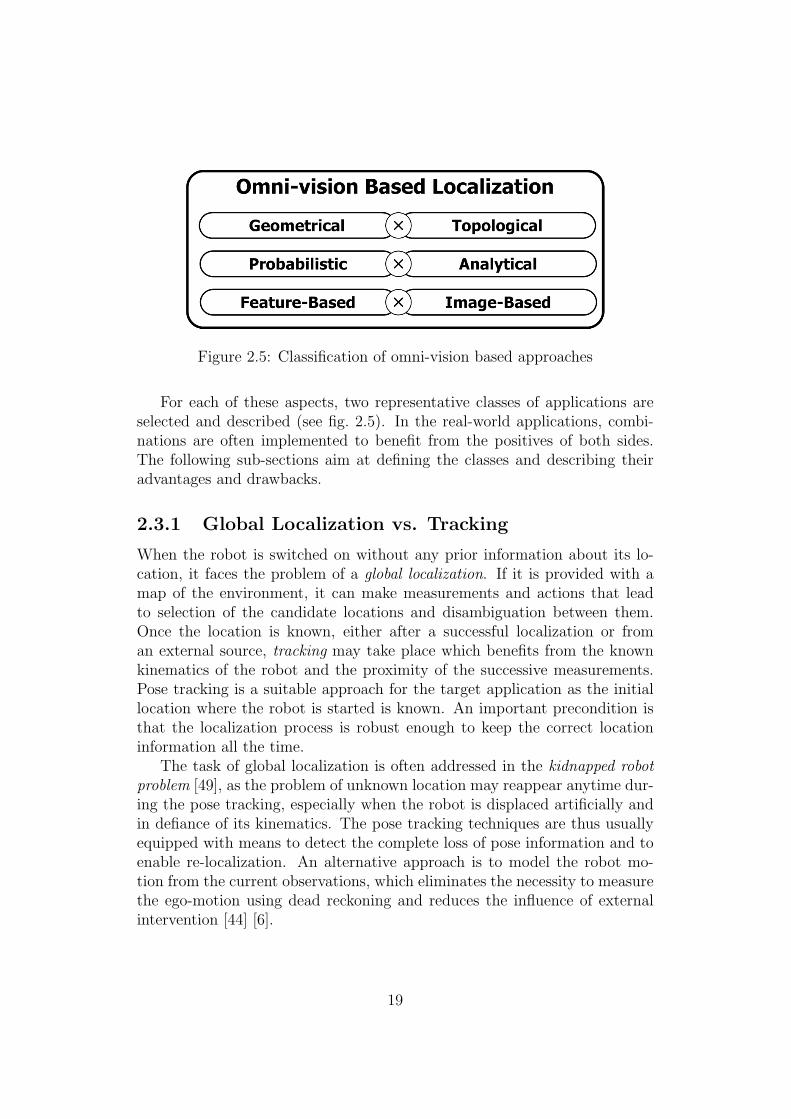
Figure 2.5: Classification of omni-vision based approaches

For each of these aspects, two representative classes of applications areselected and described (see fig. 2.5). In the real-world applications, combi-nations are often implemented to benefit from the positives of both sides.The following sub-sections aim at defining the classes and describing theiradvantages and drawbacks.

2.3.1 Global Localization vs. Tracking

When the robot is switched on without any prior information about its lo-cation, it faces the problem of a global localization. If it is provided with amap of the environment, it can make measurements and actions that leadto selection of the candidate locations and disambiguation between them.Once the location is known, either after a successful localization or froman external source, tracking may take place which benefits from the knownkinematics of the robot and the proximity of the successive measurements.Pose tracking is a suitable approach for the target application as the initiallocation where the robot is started is known. An important precondition isthat the localization process is robust enough to keep the correct locationinformation all the time.

The task of global localization is often addressed in the kidnapped robotproblem [49], as the problem of unknown location may reappear anytime dur-ing the pose tracking, especially when the robot is displaced artificially andin defiance of its kinematics. The pose tracking techniques are thus usuallyequipped with means to detect the complete loss of pose information and toenable re-localization. An alternative approach is to model the robot mo-tion from the current observations, which eliminates the necessity to measurethe ego-motion using dead reckoning and reduces the influence of externalintervention [44] [6].

19

2.3.2 Geometrical vs. Topological Approach

There are two general principles to represent the robot’s state within theworld model. A continuous, geometrical (metrical), approach describes therobot’s location using numerical terms with respect to a selected coordinatesystem. The discrete one, topological, uses specific highlighted places to rep-resent the positions and goals within the environment. This is better suitedfor applications involving human operators, as people preferably describe agoal as ’enter the second door on the left’ rather than ’follow azimuth 244for 7.29 meters, then azimuth 152 for 2.6 meters’. The metrical approach onthe other hand is more suitable when the robot is required to follow a pathwithin a specified margin [17].

In the topological approach, the world is described using a graph, wherethe nodes represent the known reference locations, and the edges correspondto the possible transitions between these nodes. The individual referencelocations are recorded during the learning (mapping) phase and contain rel-evant information that can be used for the localization (such as metricalcoordinates or semantic description of the place) together with the informa-tion that enables the robot to evaluate the similarity of current observationsto the reference ones, and thus identify the closest node.

It is also important to note, that for majority of applications the topolog-ical navigation has to be combined with some kind of metrical navigation, asmanual creation of a topological map is hardly feasible. Once the graph repre-sentation including metrical evaluation of the reference locations is recorded,a simple architecture (such as a reactive one, based only on dead reckoning)may be used to move between the individual nodes. A suitable scenario forthe topological localization is an indoor office/hallway environment, whichmaps well to a graph representation [34].

For the target operation area, and generally for open environments wherethe robot can freely move in any direction and no locations with specificimportance exist, the geometrical approach is more suitable. It is also usefulwhen the robot has to follow precisely a given path, presented as a set ofnumerical coordinates. The selection of the reference coordinate system isstraightforward for a limited known environment. For a rectangular opera-tion field a Cartesian system aligned with the two axes of the field is oftenused.

2.3.3 Probabilistic vs. Analytical Approach

An ideal solution to the localization problem is to develop sensors able toanalytically calculate the current position using only the most recent ob-servations. This is achievable with e.g. beacon-based systems, where the

20

specific landmarks in the environment can be uniquely identified and pre-cisely localized. In unmodified natural environments this is typically not thecase. Even if the vision-based systems provide less ambiguity of the landmarkobservations compared to the rangefinder-based approaches, the problem ofperceptual aliasing [34], i.e. existence of distinct but visually similar locationshas to be considered.

In most cases, the uncertainty of the robot state and its development ismodelled in the localization process. The restrictions based on the robot’skinematics help to eliminate the distant candidate locations, reduce the am-biguity, and focus the computation on the particular area of interest. Thegeneral specification of the probabilistic localization problem involves posi-tion estimates using dead-reckoning (for example with the robot’s odometry)and iterative enhancement using environment map and sensor input. Thesystem starts with an initial estimate of the robot’s location in a configu-ration space (Euclidean space whose dimension is equal to the number ofrobot’s degrees of freedom) given by a probability density function (PDF) ofthe robot’s position belief. As the robot navigates through the environment,the PDF is updated using a probabilistic model of the robot’s kinematicsand sensors. The probabilistic model of the robot’s motion is first appliedto obtain a predictive PDF representing the possible development of the ro-bot’s state. Sensor data is then used in conjunction with map to produce arefined position estimate having increased probability density about the trueposition of the robot [11].

The existing probabilistic approaches differ in their internal representa-tion of the belief and the associated update methods [10]. The Kalman filter,Markov Localization and the particle filter-based methods are some of the mostpopular approaches.

Kalman filtering [27] emerges when representing all the state and mea-surement densities by Gaussians. If all the motion and the measurementPDFs have normal distributions, and the initial state and measurement noiseare also specified as Gaussians, then the density will remain Gaussian at alltimes. It can be shown analytically that the Kalman filter is the optimalsolution to the probabilistic update rules under these assumptions [31]. Theinherent problem in this approach is that only one pose hypothesis can berepresented using a Gaussian density making the method in general unableto globally localize the robot or to recover from total localization failures [19].

This limitation has been addressed by two related families of algorithms:localization with multi-hypothesis Kalman filters and Markov localization.Multi-hypothesis Kalman filters represent beliefs using mixtures of Gaus-sians, which enables them to represent and track multiple, distinct hypothe-ses. However, to meet the Gaussian noise assumption inherent in the Kalman

21

filter, low-dimensional features have to be extracted from the sensor data,ignoring much of the information acquired by the robot’s sensors.

Markov localization algorithms [14], in contrast, represent beliefs in adiscretized manner over the space of all possible poses. There are differentmethods which can be roughly distinguished by the type of discretizationused for the representation of the state space. In the Topological Markov Lo-calization, the state space is organized according to the topological structureof the environment [46]. The coarse resolution of the state representationlimits the accuracy of the position estimates. Topological approaches typi-cally give only a rough sense as to where the robot is. In many applications,a more fine-grained position estimate is required, e.g. in environments witha simple topology but large open spaces, where accurate placement of therobot is needed.

To deal with multi-modal and non-Gaussian densities at a fine resolution,the Grid-based Markov Localization may take place [16]. A part of interestwithin the state space is discretized into a regular grid which is used asthe basis for an approximation of the PDF by a piece-wise constant function.Methods that use this type of representation are powerful, but suffer from thedisadvantages of computational overhead and a priori commitment to the sizeof the state space. In addition, the resolution and thereby also the precisionat which they can represent the state has to be fixed beforehand [10]. Definingdata structures enabling variable resolution representation of the state space,e.g. oct-trees, allow for effective utilization of memory and computationresources. However, the entire class of Markov-based approaches has beenrecently overcome by sampling-based systems.

The sampling-based representations are an obvious generalization of theMarkov localization methods. Instead of discretizing the domain of the PDFinto a fixed set of samples, it is sampled dynamically. The set of samples isdrawn randomly from the PDF so that they concentrate in the regions withhigh likelihood. A duality between the samples and the represented densityexists, which enables to apply existing update equations on the sampledPDF [48].

Particle-based representations have several key advantages over the fore-going approaches [15]:

1. In contrast to existing Kalman filtering based techniques, they are ableto represent multi-modal distributions and thus can globally localize arobot.

2. They drastically reduce the amount of memory required compared togrid-based Markov localization and can integrate measurements at aconsiderably higher frequency.

22

3. They are more accurate than Markov localization with a fixed cell size,as the state represented in the samples is not discretized.

4. They are also much easier to implement.

Monte Carlo Localization (MCL) [10] with a constant number of samplesis the probabilistic algorithm selected in this work . A fixed set of samplesis initialized at the starting location of the robot and then undergoes a pe-riodic sequence of prediction, correction and resampling phases. The entirealgorithm is described in more detail in Section 3.3.

2.3.4 Feature-Based vs. Image-Based Evaluation

One popular method for omnivision-based localization uses a similarity mea-sure defined directly over the space of original omni-directional images toevaluate the current observation. This appearance-based approach involves adatabase of images captured at the reference locations and searches for themost similar one. There are two important issues concerning this matching.Firstly, a compression is required to make the image comparison computa-tionally effective. Secondly, rotational invariance should be involved into theimage comparison, otherwise multiple rotations have to be recorded for thesame reference location.

Various methods have been developed. The principal component analysis(PCA) addresses the first issue reducing the dimensionality of the problem.The omni-directional images are treated as n-dimensional vectors where n

is the number of image pixels. An orthonormal basis of the reference im-age database is computed, which allows space-saving representation of everyimage of the training set using only a few parameters corresponding to themost discriminative vectors of the basis. PCA offers means for calculatingan optimal basis using singular value decomposition (SVD) of the covariancematrix, representing the images in a low-dimensional subspace that is an op-timal linear approximation of the original set in the least squares sense. Thedimension of the feature subspace is usually set between 10 and 15 for a gray-scale omni-directional image. Higher number of dimensions leads to betterdiscriminability but increases the risk of over-learning. Another suitable ap-proach employs a cylindrical projection of the omni-directional image. Theadvantage of this projection is in that rotation of the camera corresponds toa translation of the projected image — the azimuth of a scene point equalsto the horizontal coordinate in the rectified image. Selected componentsfrom the Fourier transform of the projected image thus provide both imagecompression and rotational invariance.

23

Although the image-based approach looks temptingly feasible, straight-forward and natural, there are several issues. One is the problem of percep-tual aliasing, e.g. in long hallways with doors similar one to another. Otherfundamental problem is the uneven influence of illumination changes andpartial occlusions on the representation of the captured image. Finally, thecreation of the database may be extremely tedious if performed manually orrequire additional metrical mapping or map geometry restoration techniqueif it is to be automatized.

Viable real-world applications extract some kind of features contained inthe image of the environment. The discussion on the usable landmarks isgiven a respective section.

2.3.5 Natural and Artificial Landmarks

A landmark is generally any feature of the environment that can be repeat-edly identified by the robot as being relevant. There is a broad range oflandmarks considering both their artificiality and relevance for the localiza-tion task. Objects ranging from purpose-built beacons and reflective or con-tractive markings to edges or corners in a human-built environment or justdistinct contours in a natural outdoor environment, all these can be used todetermine relevant position information. Also the amount of obtained infor-mation differs from precise triangulation using uniquely identified beacons torelative motion information from tracking a distinctive feature among severalsuccessive images.

The definition of landmarks used by the specific implementation is typi-cally imposed by the restrictions of the target environment. Special applica-tions posing severe requirements on robustness and reliability usually allowarbitrary modification of the environment in order to simplify the applica-tion design. This class of tasks is considered to be solved and is typicallyaddressed by engineers rather than robotics researchers. Current researchhighlights the ability to navigate in unmodified and unknown environmentsallowing the robots to extend their operation range beyond the robotic labsand workshops. Similarly, the robotic competitions tend to gradually com-plicate the navigation task by reducing the amount of artificial landmarksand limitations.

There are currently three principal domains for autonomous robot nav-igation: the exploration devices designed for operation in hardly accessiblelocations, the robots designed in the context of academic research and therobots involved in robotic competitions. All these domains involve a slightlydifferent approach to the ultimate task of unrestricted autonomous operationbased on the actual priorities.

24

It is the space program that engages the most robust and sophisticatedapplications, but various terrestrial missions as e.g. land mine elimination orrescue operations [30] also require reliable devices. It is obvious that no priormodification of the environment is applicable. The general localization innatural unmodified outdoor environment still remains a very hard problemand a large portion of human operator intervention stays involved.

An important class of research applications targets natural indoor envi-ronments. The scope of such projects is to develop fully autonomous devicesable to navigate inside any building. Besides the fact that the consideredmotion may be restricted to three degrees of freedom (within a single floor),an unmodified indoor environment also contains a large number of interest-ing landmarks, such as e.g. windows, door posts and other edges, moreovertypically rectangular. The landmarks most commonly used in the indoorenvironments are vertical edges, as they project aptly especially on omni-directional sensors, and the more general SIFT features [28], a class of imagefeatures that are invariant to image scale, rotation and translation as well asto illumination changes and affine or 3D projection.

Last but not the least, the domain of robotic competitions motivates therobotic science. The participants are presented rules, which are restrictive ina manner to encourage research and favor new solutions while leaving con-siderable space for creativity and improvements. The operation environmentis pre-defined and typically contains multiple kinds of artificial landmarks.The focus is on real-time response and reasonable robustness in order to ac-complish the given task. The robotic competitions are very important forthe development of robotics as the concurrent evolution of the game rulesand the game tactics pushes the horizons in a reasonable pace.

2.4 Related Work

Surprisingly little work exists on the omni-directional vision applied to thetask of robot localization; although it can be seen that once this approachis visited by a researcher it is rarely abandoned. Mainly the principle of fullsensoric coverage of the robot’s surroundings is very advantageous.

The annotated works are grouped by the top-level approach, i.e. appear-ance or feature based. Much of the feature-based localization work is beingdone for the RoboCup Middle Size League. These applications are given aproper subsection.

2.4.1 Appearance-Based Approach

Back in the 1996, Ishiguro and Tsuji [25] were one of the first to examine

25

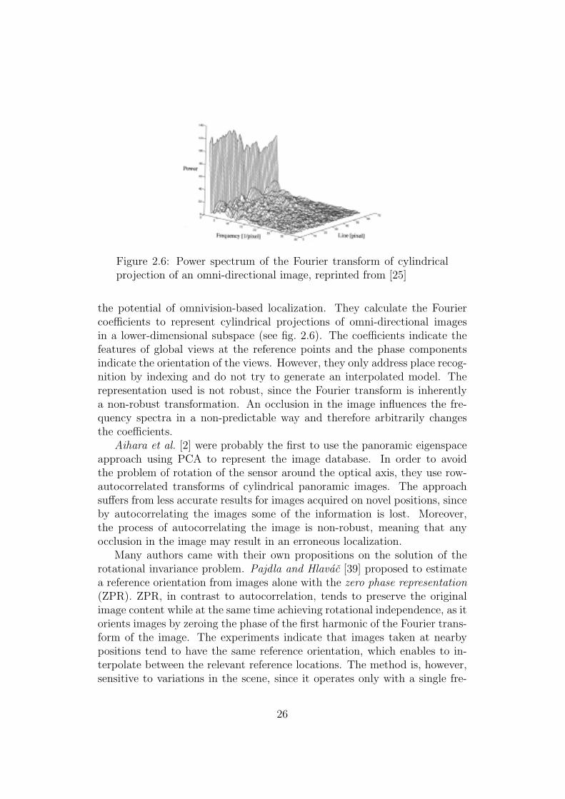
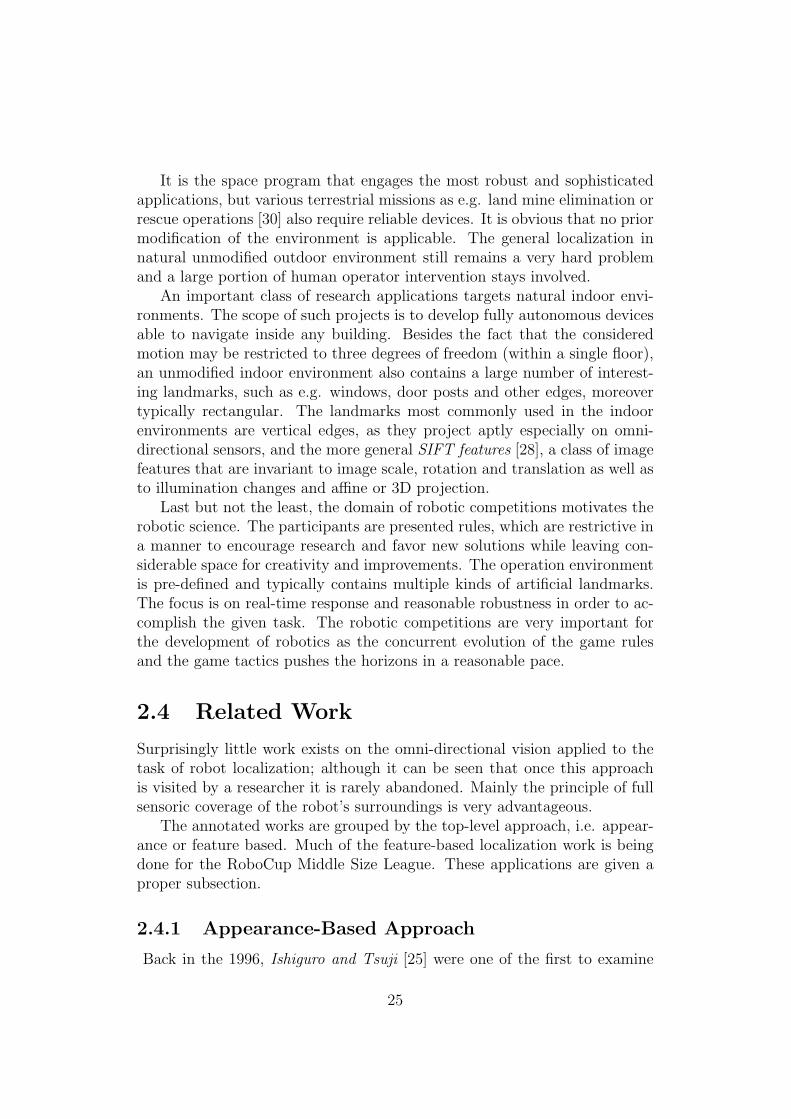
Figure 2.6: Power spectrum of the Fourier transform of cylindricalprojection of an omni-directional image, reprinted from [25]

the potential of omnivision-based localization. They calculate the Fouriercoefficients to represent cylindrical projections of omni-directional imagesin a lower-dimensional subspace (see fig. 2.6). The coefficients indicate thefeatures of global views at the reference points and the phase componentsindicate the orientation of the views. However, they only address place recog-nition by indexing and do not try to generate an interpolated model. Therepresentation used is not robust, since the Fourier transform is inherentlya non-robust transformation. An occlusion in the image influences the fre-quency spectra in a non-predictable way and therefore arbitrarily changesthe coefficients.

Aihara et al. [2] were probably the first to use the panoramic eigenspaceapproach using PCA to represent the image database. In order to avoidthe problem of rotation of the sensor around the optical axis, they use row-autocorrelated transforms of cylindrical panoramic images. The approachsuffers from less accurate results for images acquired on novel positions, sinceby autocorrelating the images some of the information is lost. Moreover,the process of autocorrelating the image is non-robust, meaning that anyocclusion in the image may result in an erroneous localization.

Many authors came with their own propositions on the solution of therotational invariance problem. Pajdla and Hlavac [39] proposed to estimatea reference orientation from images alone with the zero phase representation(ZPR). ZPR, in contrast to autocorrelation, tends to preserve the originalimage content while at the same time achieving rotational independence, as itorients images by zeroing the phase of the first harmonic of the Fourier trans-form of the image. The experiments indicate that images taken at nearbypositions tend to have the same reference orientation, which enables to in-terpolate between the relevant reference locations. The method is, however,sensitive to variations in the scene, since it operates only with a single fre-

26

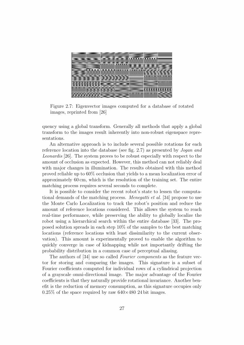
Figure 2.7: Eigenvector images computed for a database of rotatedimages, reprinted from [26]

quency using a global transform. Generally all methods that apply a globaltransform to the images result inherently into non-robust eigenspace repre-sentations.

An alternative approach is to include several possible rotations for eachreference location into the database (see fig. 2.7) as presented by Jogan andLeonardis [26]. The system proves to be robust especially with respect to theamount of occlusion as expected. However, this method can not reliably dealwith major changes in illumination. The results obtained with this methodproved reliable up to 60% occlusion that yields to a mean localization error ofapproximately 60 cm, which is the resolution of the training set. The entirematching process requires several seconds to complete.

It is possible to consider the recent robot’s state to lessen the computa-tional demands of the matching process. Menegatti et al. [34] propose to usethe Monte Carlo Localization to track the robot’s position and reduce theamount of reference locations considered. This allows the system to reachreal-time performance, while preserving the ability to globally localize therobot using a hierarchical search within the entire database [33]. The pro-posed solution spreads in each step 10% of the samples to the best matchinglocations (reference locations with least dissimilarity to the current obser-vation). This amount is experimentally proved to enable the algorithm toquickly converge in case of kidnapping while not importantly drifting theprobability distribution in a common case of perceptual aliasing.

The authors of [34] use so called Fourier components as the feature vec-tor for storing and comparing the images. This signature is a subset ofFourier coefficients computed for individual rows of a cylindrical projectionof a grayscale omni-directional image. The major advantage of the Fouriercoefficients is that they naturally provide rotational invariance. Another ben-efit is the reduction of memory consumption, as this signature occupies only0.25% of the space required by raw 640×480 24 bit images.

27

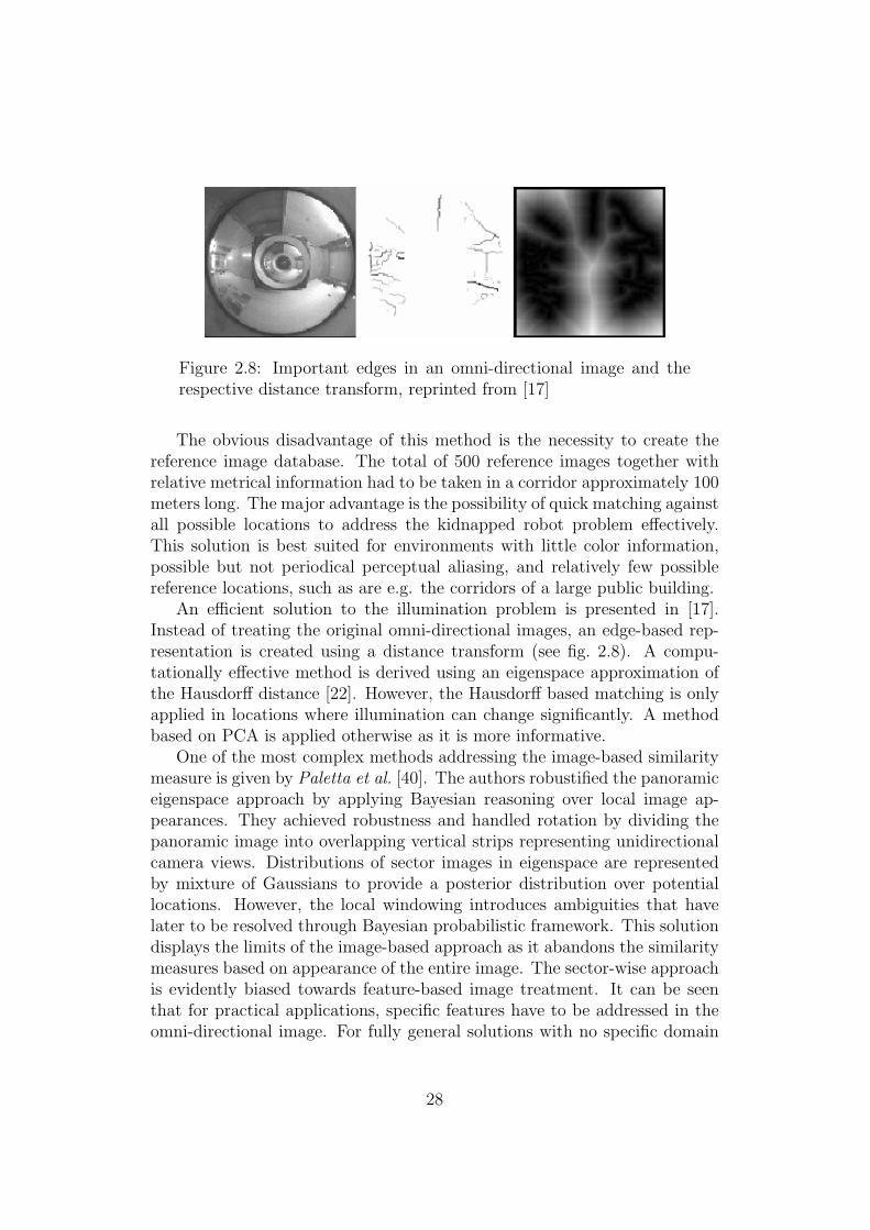
Figure 2.8: Important edges in an omni-directional image and therespective distance transform, reprinted from [17]

The obvious disadvantage of this method is the necessity to create thereference image database. The total of 500 reference images together withrelative metrical information had to be taken in a corridor approximately 100meters long. The major advantage is the possibility of quick matching againstall possible locations to address the kidnapped robot problem effectively.This solution is best suited for environments with little color information,possible but not periodical perceptual aliasing, and relatively few possiblereference locations, such as are e.g. the corridors of a large public building.

An efficient solution to the illumination problem is presented in [17].Instead of treating the original omni-directional images, an edge-based rep-resentation is created using a distance transform (see fig. 2.8). A compu-tationally effective method is derived using an eigenspace approximation ofthe Hausdorff distance [22]. However, the Hausdorff based matching is onlyapplied in locations where illumination can change significantly. A methodbased on PCA is applied otherwise as it is more informative.

One of the most complex methods addressing the image-based similaritymeasure is given by Paletta et al. [40]. The authors robustified the panoramiceigenspace approach by applying Bayesian reasoning over local image ap-pearances. They achieved robustness and handled rotation by dividing thepanoramic image into overlapping vertical strips representing unidirectionalcamera views. Distributions of sector images in eigenspace are representedby mixture of Gaussians to provide a posterior distribution over potentiallocations. However, the local windowing introduces ambiguities that havelater to be resolved through Bayesian probabilistic framework. This solutiondisplays the limits of the image-based approach as it abandons the similaritymeasures based on appearance of the entire image. The sector-wise approachis evidently biased towards feature-based image treatment. It can be seenthat for practical applications, specific features have to be addressed in theomni-directional image. For fully general solutions with no specific domain

28

Figure 2.9: Minimum free space estimation, reprinted from [52]

of operation, generic invariant features should be taken into account insteadof aspiring for appearance-based invariance.

2.4.2 Feature-Based Approach

Returning back to the 1995, one of the first practical experiments with omni-directional navigation already uses a feature based approach. In the work ofYagi et al. [52] a Conic Projection Image Sensor (COPIS) detects and tracksvertical edges in the environment. The sensor contains a conical mirror,which projects the vertical edges to radial lines in the image, and a TVcamera, which sends the images wirelessly to a control computer. Becausethe COPIS sensor is omni-directional and the environment is constructedto be populated with vertical lines, a large number of azimuth readings areobtained surrounding the robot. The system is capable both of improvingthe rough location estimate using a map of known features and of detectingand recording a new feature. A simple sort algorithm is used to maintain thelist of known edges. The locations of unknown obstacles are estimated bymonitoring loci of azimuth angles of the vertical edges. The coordinates ofnew edges are corrected using triangulation from successive readings. A largeerror occurs in the front region of the robot when the robot moves straightahead, but the error diminishes when the robot changes direction.

Known vertical edges are used to define the minimum free space (seefig. 2.9), a wire occupancy map of the environment created connecting theadjacent vertical edges and verifying the candidate surfaces using an acousticsensor. An ultrasonic sensor is used if and only if the robot is required topass through a candidate surface to verify if it is a real one. This is one ofthe major drawbacks of edge-based navigation — the configuration of objectsurfaces can only be estimated and need to be verified otherwise.

The image analysis was implemented on an image processor and was ableto process about 1 fps including the time needed for communication. Thespeed of the robot was about 5 cm per second and the localization error inan artificial box-like test environment ranged from 3 to 7 cm.

In the work of Dellaert et al. from 1999 [10] the idea of Monte Carlo Lo-calization (MCL) crystallized. This localization technique was presented as

29

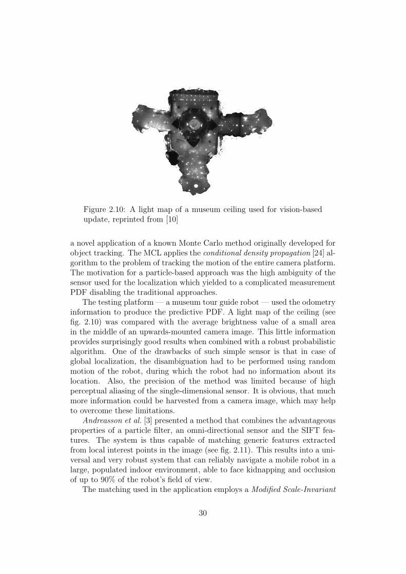
Figure 2.10: A light map of a museum ceiling used for vision-basedupdate, reprinted from [10]

a novel application of a known Monte Carlo method originally developed forobject tracking. The MCL applies the conditional density propagation [24] al-gorithm to the problem of tracking the motion of the entire camera platform.The motivation for a particle-based approach was the high ambiguity of thesensor used for the localization which yielded to a complicated measurementPDF disabling the traditional approaches.

The testing platform — a museum tour guide robot — used the odometryinformation to produce the predictive PDF. A light map of the ceiling (seefig. 2.10) was compared with the average brightness value of a small areain the middle of an upwards-mounted camera image. This little informationprovides surprisingly good results when combined with a robust probabilisticalgorithm. One of the drawbacks of such simple sensor is that in case ofglobal localization, the disambiguation had to be performed using randommotion of the robot, during which the robot had no information about itslocation. Also, the precision of the method was limited because of highperceptual aliasing of the single-dimensional sensor. It is obvious, that muchmore information could be harvested from a camera image, which may helpto overcome these limitations.

Andreasson et al. [3] presented a method that combines the advantageousproperties of a particle filter, an omni-directional sensor and the SIFT fea-tures. The system is thus capable of matching generic features extractedfrom local interest points in the image (see fig. 2.11). This results into a uni-versal and very robust system that can reliably navigate a mobile robot in alarge, populated indoor environment, able to face kidnapping and occlusionof up to 90% of the robot’s field of view.

The matching used in the application employs a Modified Scale-Invariant

30

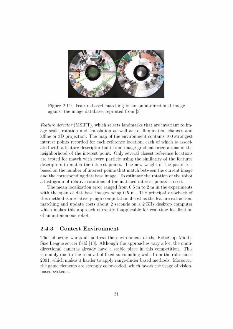
Figure 2.11: Feature-based matching of an omni-directional imageagainst the image database, reprinted from [3]

Feature detector (MSIFT), which selects landmarks that are invariant to im-age scale, rotation and translation as well as to illumination changes andaffine or 3D projection. The map of the environment contains 100 strongestinterest points recorded for each reference location, each of which is associ-ated with a feature descriptor built from image gradient orientations in theneighborhood of the interest point. Only several closest reference locationsare tested for match with every particle using the similarity of the featuresdescriptors to match the interest points. The new weight of the particle isbased on the number of interest points that match between the current imageand the corresponding database image. To estimate the rotation of the robota histogram of relative rotations of the matched interest points is used.

The mean localization error ranged from 0.5 m to 2 m in the experimentswith the span of database images being 0.5 m. The principal drawback ofthis method is a relatively high computational cost as the feature extraction,matching and update costs about 2 seconds on a 2GHz desktop computerwhich makes this approach currently inapplicable for real-time localizationof an autonomous robot.

2.4.3 Contest Environment

The following works all address the environment of the RoboCup MiddleSize League soccer field [13]. Although the approaches vary a lot, the omni-directional cameras already have a stable place in this competition. Thisis mainly due to the removal of fixed surrounding walls from the rules since2001, which makes it harder to apply range-finder based methods. Moreover,the game elements are strongly color-coded, which favors the usage of vision-based systems.

31

Figure 2.12: Bird’s eye view of the RoboCup field with the estimatedpairs of line segments highlighted, reprinted from [29]

Marques and Lima [29] propose to extract the geometrical features froma bird eye’s perspective of the environment. They describe a general ap-proach for tracking straight line segments on the floor and an application toanalytical localization on a RoboCup soccer field. The method benefits froma mirror profile that realizes a constant horizontal resolution projection andthus preserves the geometry of the ground plane(see fig. 2.12).

The transition pixels denoting interesting features in the acquired imageare processed using Hough transform (HT) [21] to detect straight linear pat-terns of the floor. A fixed count of most distinct straight lines is picked andall pairs made out of these lines are classified for relevance using a prioriknowledge of the environment geometrics. This step is used to highlightpairs of parallel lines enclosing an expected gap. The common direction ofthe most relevant pair is used to pick the remaining parallel lines. These se-lected lines are then correlated with a corresponding set of model features tofind the best match. The selection and correlation process is then repeatedwith the remaining non-parallel lines. Two sets of six and five parallel linesof a RoboCup soccer field were used in the practical application. Typicalposition errors ranged from 0 to 10 cm.

This approach is functional and robust mainly due to the integrativefashion of the HT. On the other hand, ignoring the continuity of the robotstate throws away much of the information reusable in the next localizationstep. This may especially prove derogative in real-world environment withconsiderable distortion and occlusion influences. The analytical approachrisks sudden fallouts, which could be avoided using an uncertainty-modellingapproach.

Sekimori et al. [42] present an analytical approach to the localizationproblem on a RoboCup field based on a single tracked landmark — thegreen rectangular shape of the entire playing field floor. The method startswith image pre-processing that extracts a convex hull of the floor projection.

32

Figure 2.13: The process of estimating playing field position usingthe green floor segment, reprinted from [42]

This reduces the effect of occlusions on the floor shape. The floor outlineis then projected back to the coordinate system of the ground plane andgeometric moments of the shape are calculated to obtain a rough match withthe field model. Least-squares optimization is then used for best fit withthe model (see fig. 2.13). The rotation and shift of the observed landmarkdefine the current robot’s coordinates with the only ambiguity of field centralsymmetry. If the color of goal is observed it solves this ambiguity, otherwisethe most recent solution is chosen.

Extending the initial idea using probabilistic refinement, a robust solutionis achieved [43]. The global position information can be easily reformulatedin a form suitable for the Kalman filter. The self position estimation isupdated by dead reckoning using odometry and the belief is improved by thevision-based self-position observation described above. The Kalman filteringhelps to improve the localization performance, which would otherwise sufferfrom quantization errors, occlusions and noise in the images.

The resulting method seems to be robust and reliable. The only short-coming may be the necessity to always fit the entire field into the view of theomni-directional camera. This greatly reduces the resolution of the sensorbut there are means to address this issue if required [32].

An interesting hybrid of the analytical and probabilistic approaches ispresented in [36]. The method uses ambiguous landmark observations of

33

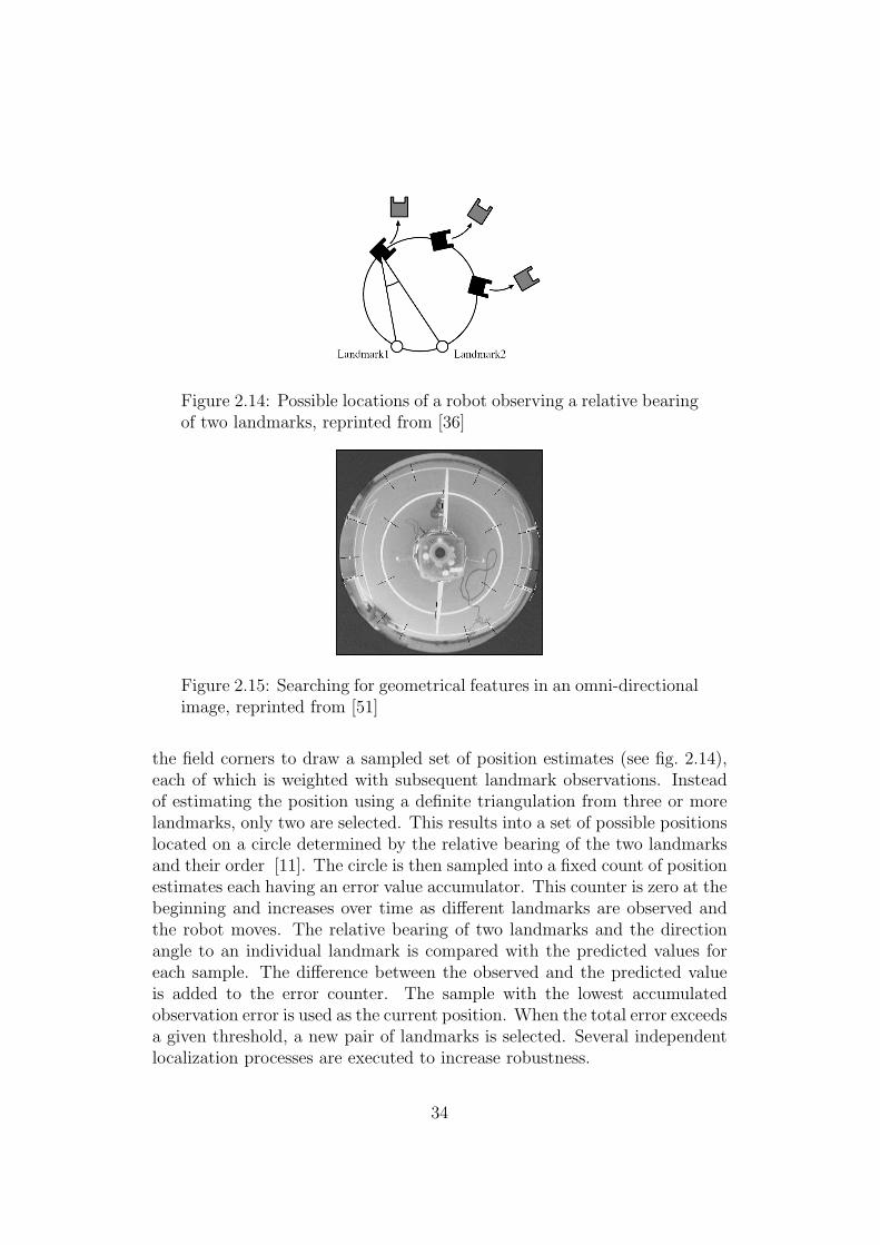
Figure 2.14: Possible locations of a robot observing a relative bearingof two landmarks, reprinted from [36]

Figure 2.15: Searching for geometrical features in an omni-directionalimage, reprinted from [51]

the field corners to draw a sampled set of position estimates (see fig. 2.14),each of which is weighted with subsequent landmark observations. Insteadof estimating the position using a definite triangulation from three or morelandmarks, only two are selected. This results into a set of possible positionslocated on a circle determined by the relative bearing of the two landmarksand their order [11]. The circle is then sampled into a fixed count of positionestimates each having an error value accumulator. This counter is zero at thebeginning and increases over time as different landmarks are observed andthe robot moves. The relative bearing of two landmarks and the directionangle to an individual landmark is compared with the predicted values foreach sample. The difference between the observed and the predicted valueis added to the error counter. The sample with the lowest accumulatedobservation error is used as the current position. When the total error exceedsa given threshold, a new pair of landmarks is selected. Several independentlocalization processes are executed to increase robustness.

34

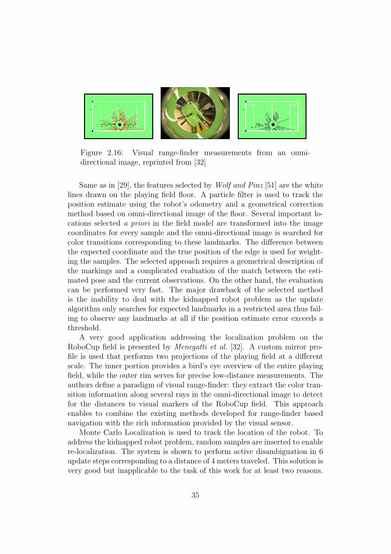
Figure 2.16: Visual range-finder measurements from an omni-directional image, reprinted from [32]

Same as in [29], the features selected by Wolf and Pinz [51] are the whitelines drawn on the playing field floor. A particle filter is used to track theposition estimate using the robot’s odometry and a geometrical correctionmethod based on omni-directional image of the floor. Several important lo-cations selected a priori in the field model are transformed into the imagecoordinates for every sample and the omni-directional image is searched forcolor transitions corresponding to these landmarks. The difference betweenthe expected coordinate and the true position of the edge is used for weight-ing the samples. The selected approach requires a geometrical description ofthe markings and a complicated evaluation of the match between the esti-mated pose and the current observations. On the other hand, the evaluationcan be performed very fast. The major drawback of the selected methodis the inability to deal with the kidnapped robot problem as the updatealgorithm only searches for expected landmarks in a restricted area thus fail-ing to observe any landmarks at all if the position estimate error exceeds athreshold.

A very good application addressing the localization problem on theRoboCup field is presented by Menegatti et al. [32]. A custom mirror pro-file is used that performs two projections of the playing field at a differentscale. The inner portion provides a bird’s eye overview of the entire playingfield, while the outer rim serves for precise low-distance measurements. Theauthors define a paradigm of visual range-finder: they extract the color tran-sition information along several rays in the omni-directional image to detectfor the distances to visual markers of the RoboCup field. This approachenables to combine the existing methods developed for range-finder basednavigation with the rich information provided by the visual sensor.

Monte Carlo Localization is used to track the location of the robot. Toaddress the kidnapped robot problem, random samples are inserted to enablere-localization. The system is shown to perform active disambiguation in 6update steps corresponding to a distance of 4 meters traveled. This solution isvery good but inapplicable to the task of this work for at least two reasons.

35

Firstly, the target environment has a periodic color pattern, which wouldmake a visual range-finder very ambiguous. Secondly, such custom mirrorprofile is difficult to obtain.

2.5 Proposed Solution

Firstly, it has to be noted that a customized approach must be derived fora very specific target environment to make the solution effective in termsof development and computational costs. The applications noted above areall performing well in their own environments but are rarely general enoughto be simply reproduced. On the other hand, selecting a too complex andgeneric approach would make the resulting application hardly competitive inthe terms of processing speed.

The scope of this work is to design and implement a localization mod-ule for a mobile robot operating in the Eurobotopen 2005 contest environ-ment [12]. The following sections first specify the available features of thegiven environment, followed by the presentation of the prototype solutionand its contribution.

2.5.1 Target Environment

The operation field of the Eurobotopen 2005 contest is a rectangular area ofapproximately 2.1×3.6 meters consisting of two fields with a brown-beige30×30 cm checkerboard pattern separated by a blue ditch and surroundedby a white border. The central ditch is 60 cm wide and is 3.6 cm below thelevel of the playing field floor. It is separated from the two floors by a glossywhite line. The construction of the target robotic platform enables it onlyto cross the ditch using one of the two beige bridges, positioned randomlybefore the start of a match. The detailed description of the playing field andan overview of the game rules can be found in the Appendix A.2.

Visual features usable for the localization include the checkerboard pat-tern, the blue ditch with the randomly positioned beige bridges and the whiteborders denoting the limits of the checkerboard fields and the ditch.

The localization task is complicated by the fact that the playing field ispopulated with additional elements that tend to confuse the visual sensorby occluding the expected landmarks and creating false ones. These arenamely the game elements, such as are the 15 green and 15 red skittles andtwo black bowls. Moreover, the solution must expect very frequent influencesfrom other robots operating on the playing field — physical robot interactionsare very frequent in this contest.

36

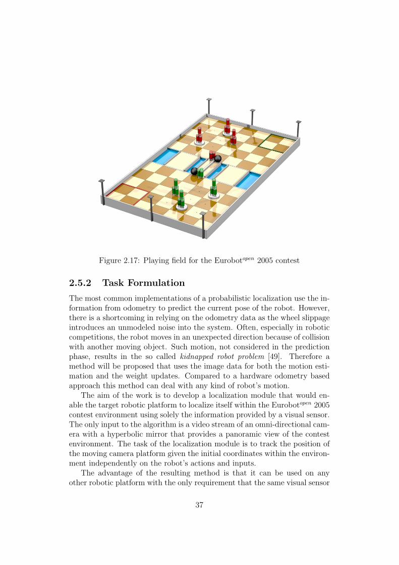
Figure 2.17: Playing field for the Eurobotopen 2005 contest

2.5.2 Task Formulation

The most common implementations of a probabilistic localization use the in-formation from odometry to predict the current pose of the robot. However,there is a shortcoming in relying on the odometry data as the wheel slippageintroduces an unmodeled noise into the system. Often, especially in roboticcompetitions, the robot moves in an unexpected direction because of collisionwith another moving object. Such motion, not considered in the predictionphase, results in the so called kidnapped robot problem [49]. Therefore amethod will be proposed that uses the image data for both the motion esti-mation and the weight updates. Compared to a hardware odometry basedapproach this method can deal with any kind of robot’s motion.

The aim of the work is to develop a localization module that would en-able the target robotic platform to localize itself within the Eurobotopen 2005contest environment using solely the information provided by a visual sensor.The only input to the algorithm is a video stream of an omni-directional cam-era with a hyperbolic mirror that provides a panoramic view of the contestenvironment. The task of the localization module is to track the position ofthe moving camera platform given the initial coordinates within the environ-ment independently on the robot’s actions and inputs.

The advantage of the resulting method is that it can be used on anyother robotic platform with the only requirement that the same visual sensor

37

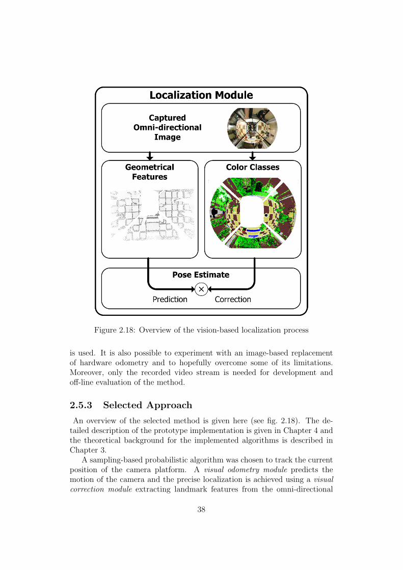
Figure 2.18: Overview of the vision-based localization process

is used. It is also possible to experiment with an image-based replacementof hardware odometry and to hopefully overcome some of its limitations.Moreover, only the recorded video stream is needed for development andoff-line evaluation of the method.

2.5.3 Selected Approach

An overview of the selected method is given here (see fig. 2.18). The de-tailed description of the prototype implementation is given in Chapter 4 andthe theoretical background for the implemented algorithms is described inChapter 3.

A sampling-based probabilistic algorithm was chosen to track the currentposition of the camera platform. A visual odometry module predicts themotion of the camera and the precise localization is achieved using a visualcorrection module extracting landmark features from the omni-directional

38

image. A bird’s eye view transform is applied on the acquired image torectify the geometry of the rectangular playing field landmarks.

Instead of trying to evaluate the relative position of the entire playingfield, which would be very hard due to the fact that the playing field sur-roundings are not defined, easily detectable features of the playing field areextracted and tracked to determine the relative motion of the robot. A prob-abilistic update is then applied to refine this position estimate.

The odometry module tracks the boundaries of the playing field land-marks. A relative position within one checkerboard square is estimated bydetecting the orientation and shift of the rectangular grid formed by the indi-vidual checkerboard squares in the rectified image. This relative informationis continually tracked to get the global position estimate. Because of theperiodicity of the basic pattern, an ambiguity in the motion estimation hasto be solved imposing an upper bound on the robot’s speed.

To correct for position estimate errors induced by the image noise, oc-clusions, reflections, and especially distortions caused by the camera tilt, theraw accumulated position estimate is periodically corrected in the probabilis-tic framework using a map of the playing field colors and a sparse pixel-wisecomparison with the color-classified omni-directional image.

This is an alternative approach opposing the most common modalitiesconsisting of precise odometry and range-finder sensors. One of the motiva-tions is to examine the possibilities of the visual odometry and to offer anaffordable option to the costly sensors used in current robotic applications.The major benefit of the probabilistic approach is that additional sensorscan be easily integrated into the existing framework to increase precisionand robustness. This would enable e.g. to enhance the developed solutionwith hardware odometry if available on the target platform or to replace thevisual odometry at all if no suitable landmarks exist within an alternativeenvironment.

39

Chapter 3

Theory

This chapter presents a theoretical background for the omni-directional im-age formation, color classification and probabilistic localization algorithmsemployed in the prototype implementation.

3.1 Omni-directional Vision

The projection model used in this work consists of the perspective cameraprojection combined with a curved reflexive surface.

In the perspective projection model, the three-dimensional feature pointsare projecting onto an image plane with perspective rays originating at thecenter of projection (COP), which would lie within the physical camera. Theorigin of the coordinate system is taken to be the COP and the focal length,f is the distance from the COP to the image plane along the optical axis,which is aligned with the ~z axis.

The perspective projection of a point (x, y, z)T in the world coordinatesto a point (u, v)T in the image coordinates is performed by(

uv

)=

(xy

)f

z

In a catadioptric configuration, the camera is combined with a curvedmirror to increase the field-of-view of the sensor. The mirror profile is arotationally symmetrical surface described by a surface function z(x) — thesurface is constructed by rotating the graph of z(x) around the optical axis.Depending on the shape of the surface equation, the mirror profiles can beroughly classified as single viewpoint (SVP), e.g. hyperbolic, and non-singleviewpoint (Non-SVP), e.g. spherical or conic (see fig. 3.1). The advantageof a SVP profile is that in certain camera configuration it reflects the rayspassing the camera COP such that they all seem to originate in a single point

40

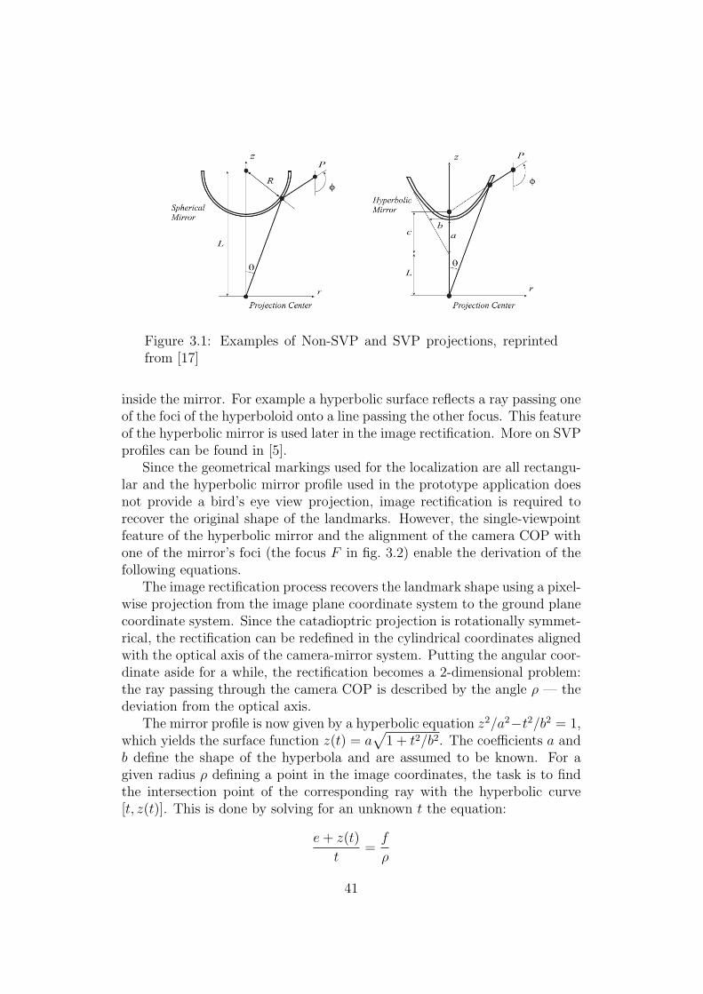
Figure 3.1: Examples of Non-SVP and SVP projections, reprintedfrom [17]

inside the mirror. For example a hyperbolic surface reflects a ray passing oneof the foci of the hyperboloid onto a line passing the other focus. This featureof the hyperbolic mirror is used later in the image rectification. More on SVPprofiles can be found in [5].

Since the geometrical markings used for the localization are all rectangu-lar and the hyperbolic mirror profile used in the prototype application doesnot provide a bird’s eye view projection, image rectification is required torecover the original shape of the landmarks. However, the single-viewpointfeature of the hyperbolic mirror and the alignment of the camera COP withone of the mirror’s foci (the focus F in fig. 3.2) enable the derivation of thefollowing equations.

The image rectification process recovers the landmark shape using a pixel-wise projection from the image plane coordinate system to the ground planecoordinate system. Since the catadioptric projection is rotationally symmet-rical, the rectification can be redefined in the cylindrical coordinates alignedwith the optical axis of the camera-mirror system. Putting the angular coor-dinate aside for a while, the rectification becomes a 2-dimensional problem:the ray passing through the camera COP is described by the angle ρ — thedeviation from the optical axis.

The mirror profile is now given by a hyperbolic equation z2/a2−t2/b2 = 1,which yields the surface function z(t) = a

√1 + t2/b2. The coefficients a and

b define the shape of the hyperbola and are assumed to be known. For agiven radius ρ defining a point in the image coordinates, the task is to findthe intersection point of the corresponding ray with the hyperbolic curve[t, z(t)]. This is done by solving for an unknown t the equation:

e + z(t)

t=

f

ρ

41

Figure 3.2: Schematic for the ground plane projection and rectifica-tion

The solution of this equation is:

t =2ab2ρf

b2f 2 − a2ρ2

Because of the single-viewpoint feature of the hyperbolic profile, the pointof intersection with the ground plane [r,−h] can be evaluated using trianglesimilarity. This is because the reflected ray is on a line connecting the innermirror focus [0, e] and the reflection point [t, z(t)] (see fig. 3.2).

Note that in the implementation the transformation is pre-calculated andstored in a look-up table to increase the execution speed.

3.2 Color perception

Fast and robust color classification is an important part of an applicationdetecting visual landmarks determined by their color. A special algorithmexists that addresses the classification issue for robotic applications wherethe processing speed is an important factor [8].

Objects uniformly painted by the same color are not represented by anequal RGB color when captured by a camera. This is due to the effect ofillumination on the hue and brightness of the reflected light. It is mainly

42

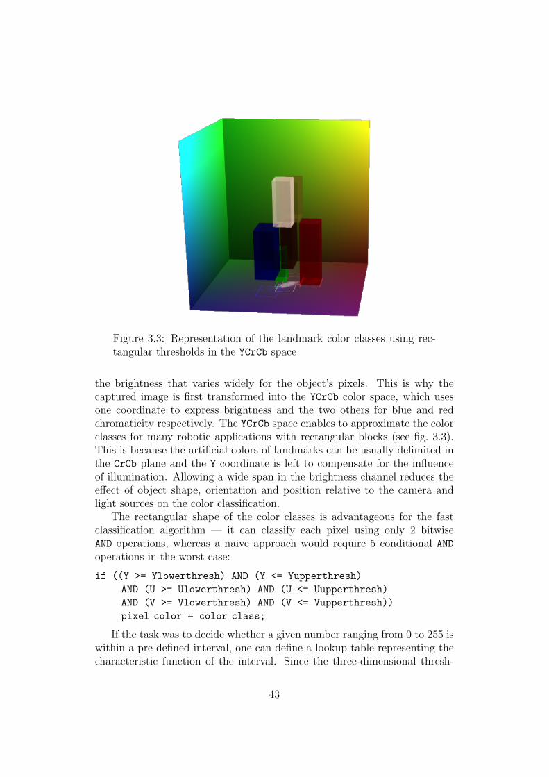
Figure 3.3: Representation of the landmark color classes using rec-tangular thresholds in the YCrCb space

the brightness that varies widely for the object’s pixels. This is why thecaptured image is first transformed into the YCrCb color space, which usesone coordinate to express brightness and the two others for blue and redchromaticity respectively. The YCrCb space enables to approximate the colorclasses for many robotic applications with rectangular blocks (see fig. 3.3).This is because the artificial colors of landmarks can be usually delimited inthe CrCb plane and the Y coordinate is left to compensate for the influenceof illumination. Allowing a wide span in the brightness channel reduces theeffect of object shape, orientation and position relative to the camera andlight sources on the color classification.

The rectangular shape of the color classes is advantageous for the fastclassification algorithm — it can classify each pixel using only 2 bitwiseAND operations, whereas a naive approach would require 5 conditional ANDoperations in the worst case:

if ((Y >= Ylowerthresh) AND (Y <= Yupperthresh)

AND (U >= Ulowerthresh) AND (U <= Uupperthresh)

AND (V >= Vlowerthresh) AND (V <= Vupperthresh))

pixel color = color class;

If the task was to decide whether a given number ranging from 0 to 255 iswithin a pre-defined interval, one can define a lookup table representing thecharacteristic function of the interval. Since the three-dimensional thresh-

43

old can be represented as a product of three interval-defined subspaces, theclassification of one pixel can be performed using 3 lookups:

pixel in class = YClass[Y] AND UClass[U] AND VClass[V];

For best performance, all the color classes can be evaluated at once. Ifthe lookup tables are made of 32-bit integers, 32 color classes can be stored,one in each bit. The bitwise AND identifies all the color classes a pixel belongsto making the respective bit set.

3.3 Monte Carlo Localization

In a probabilistic localization framework [10], the robot state at a currenttime-step k is estimated given knowledge about the initial state and all mea-surements Zk = {zk, i = 1..k} up to the current time. The robot state isgiven by a vector xk = [x, y, θ]T comprising the position and orientation ofthe robot. The estimation problem is an instance of the Bayesian filteringproblem where the posterior density p(xk|Zk) of the current state conditionedon all measurements is constructed. In the Bayesian approach, this proba-bility density function (PDF) holds all the knowledge that is available aboutthe state xk. In sampling based methods, the density is approximated bya set of N random weighted samples or particles Sk = {(si

k, wik); i = 1..N}

drawn from it. Each sik stands for one possible state of the robot and the wi

k

expresses the probability of the current state being sik. The current position

can be estimated from this representation, e.g. as a weighted average of allsamples.

To localize the robot, the goal is to recursively compute at each time-stepk the density p(xk|Zk) working with the set of samples Sk that is drawn fromit. This is done in two phases, the prediction and the update.

3.3.1 Prediction

In the first phase a motion model is used to predict the current position of therobot in the form of a predictive PDF p(xk|Zk−1), taking only motion intoaccount. The current state xk is assumed to depend only on the previous statexk−1 and a known control input uk−1. The motion model is thus specifiedas a conditional density p(xk|xk−1;uk−1). The predictive density over xk isthen obtained by integration:

p(xk|Zk−1) =

∫p(xk|xk−1;uk−1) p(xk−1|Zk−1) dxk−1

44

In the implementation of a particle filter, the motion model is appliedto each of the particles si

k−1 computed in the previous iteration obtaining anew set S ′

k that approximates a random sample from the predictive densityp(xk|Zk−1):

for each particle sik−1:

draw one sample s′ik from p(xk|sik−1; uk−1)

3.3.2 Update

In the second phase the position estimate obtained in the form of a predictivePDF is updated using a measurement model of the current sensor readingsto obtain the posterior PDF p(xk|Zk). The measurement zk is assumed tobe conditionally independent of earlier measurements Zk−1 given xk. Themeasurement model is expressed in terms of a likelihood p(zk|xk). Thisterm denotes the likelihood of the state xk given that zk was observed. Theposterior density over xk is obtained using Bayes’ theorem:

p(xk|Zk) =p(zk|xk) p(xk|Zk−1)

p(zk|Zk−1)

For a particle filter, this update consists of two steps. First the weightsare corrected according to the measurement zk. Then the particle set isresampled to represent the new density p(xk|Zk).

All the samples in the predictive set S ′k are updated by the likelihood of

s′ik given zk, i.e. weighted by:

wik = p(zk|s′ik) wi

k−1

The new set Sk is then obtained by resampling from this weighted set.All the weights are first normalized so that

∑i w

ik = N . The resampling

then reproduces the samples s′ik having a high weight associated with themreplacing those with a low weight. This addresses the problem of a continualdegeneration of the sampled PDF. The sample set must be updated to removeinsignificant samples and give place to the promising ones. In doing so a newset Sk is obtained that approximates a random sample from p(xk|Zk):

for i = 1..N:

if wik > 2 draw two Sk samples from p(xk|s′ik)

else if wik < 0.5 drop the sample s′ik

else if |Sk| < N draw one Sk sample from p(xk|s′ik)

45

After the update phase the process is repeated recursively.At time k = 0 the knowledge about the initial state x0 is assumed to

be available in the form of a density p(x0). The particle filter starts with arandom set of samples S0 = si

0 drawn from this prior density. In the posetracking task, the density p(x0) represents a narrow distribution around theknown initial pose.

46

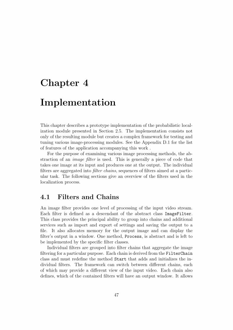
Chapter 4

Implementation

This chapter describes a prototype implementation of the probabilistic local-ization module presented in Section 2.5. The implementation consists notonly of the resulting module but creates a complex framework for testing andtuning various image-processing modules. See the Appendix D.1 for the listof features of the application accompanying this work .

For the purpose of examining various image processing methods, the ab-straction of an image filter is used. This is generally a piece of code thattakes one image at its input and produces one at the output. The individualfilters are aggregated into filter chains, sequences of filters aimed at a partic-ular task. The following sections give an overview of the filters used in thelocalization process.

4.1 Filters and Chains

An image filter provides one level of processing of the input video stream.Each filter is defined as a descendant of the abstract class ImageFilter.This class provides the principal ability to group into chains and additionalservices such as import and export of settings and saving the output to afile. It also allocates memory for the output image and can display thefilter’s output in a window. One method, Process, is abstract and is left tobe implemented by the specific filter classes.

Individual filters are grouped into filter chains that aggregate the imagefiltering for a particular purpose. Each chain is derived from the FilterChainclass and must redefine the method Start that adds and initializes the in-dividual filters. The framework can switch between different chains, eachof which may provide a different view of the input video. Each chain alsodefines, which of the contained filters will have an output window. It allows

47

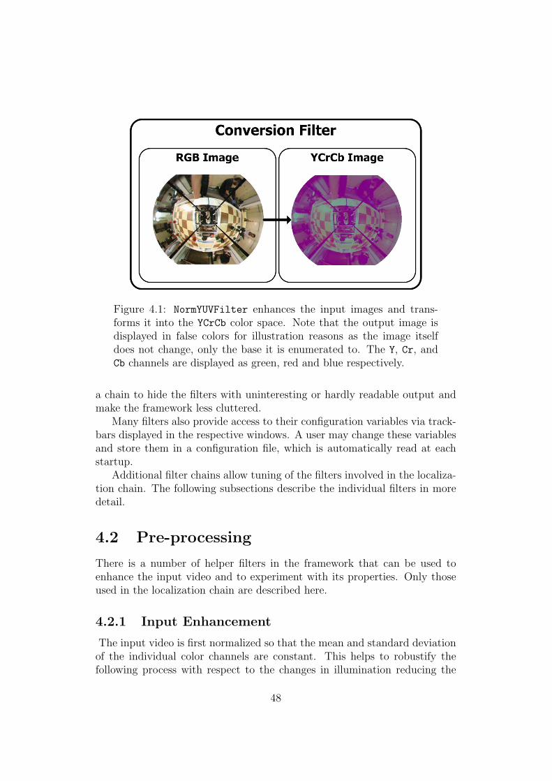
Figure 4.1: NormYUVFilter enhances the input images and trans-forms it into the YCrCb color space. Note that the output image isdisplayed in false colors for illustration reasons as the image itselfdoes not change, only the base it is enumerated to. The Y, Cr, andCb channels are displayed as green, red and blue respectively.

a chain to hide the filters with uninteresting or hardly readable output andmake the framework less cluttered.

Many filters also provide access to their configuration variables via track-bars displayed in the respective windows. A user may change these variablesand store them in a configuration file, which is automatically read at eachstartup.

Additional filter chains allow tuning of the filters involved in the localiza-tion chain. The following subsections describe the individual filters in moredetail.

4.2 Pre-processing

There is a number of helper filters in the framework that can be used toenhance the input video and to experiment with its properties. Only thoseused in the localization chain are described here.

4.2.1 Input Enhancement

The input video is first normalized so that the mean and standard deviationof the individual color channels are constant. This helps to robustify thefollowing process with respect to the changes in illumination reducing the

48

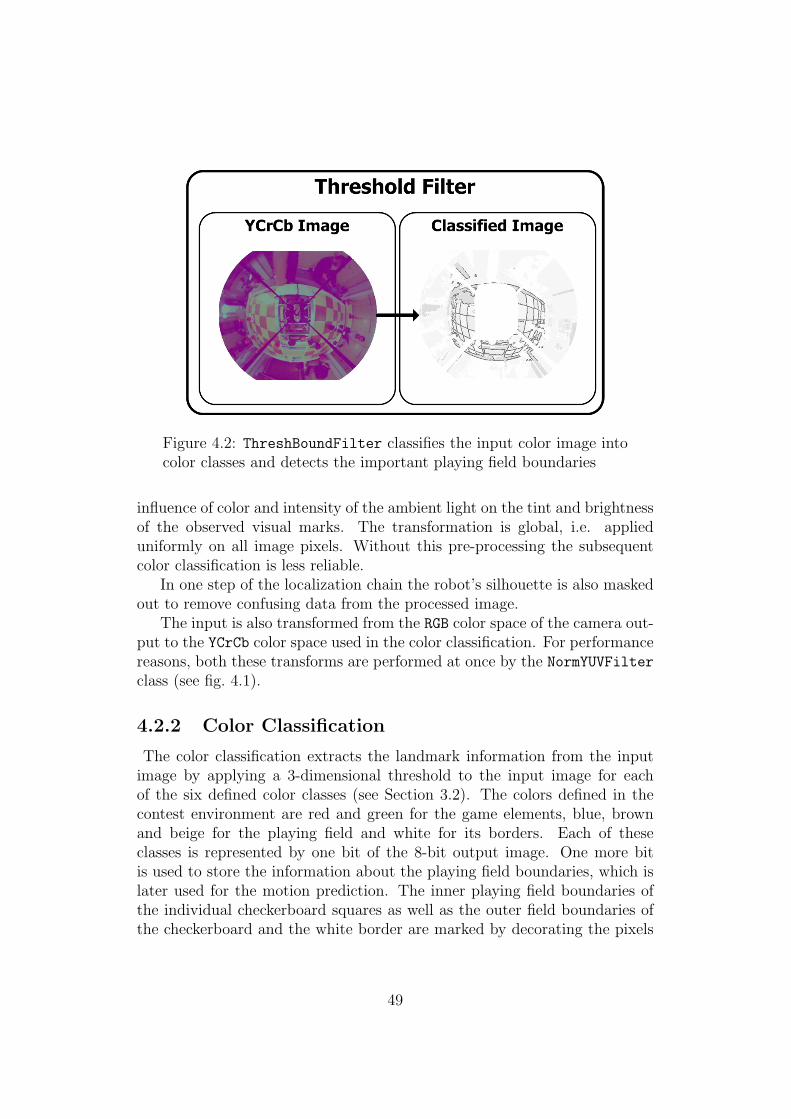
Figure 4.2: ThreshBoundFilter classifies the input color image intocolor classes and detects the important playing field boundaries

influence of color and intensity of the ambient light on the tint and brightnessof the observed visual marks. The transformation is global, i.e. applieduniformly on all image pixels. Without this pre-processing the subsequentcolor classification is less reliable.

In one step of the localization chain the robot’s silhouette is also maskedout to remove confusing data from the processed image.

The input is also transformed from the RGB color space of the camera out-put to the YCrCb color space used in the color classification. For performancereasons, both these transforms are performed at once by the NormYUVFilterclass (see fig. 4.1).

4.2.2 Color Classification

The color classification extracts the landmark information from the inputimage by applying a 3-dimensional threshold to the input image for eachof the six defined color classes (see Section 3.2). The colors defined in thecontest environment are red and green for the game elements, blue, brownand beige for the playing field and white for its borders. Each of theseclasses is represented by one bit of the 8-bit output image. One more bitis used to store the information about the playing field boundaries, which islater used for the motion prediction. The inner playing field boundaries ofthe individual checkerboard squares as well as the outer field boundaries ofthe checkerboard and the white border are marked by decorating the pixels

49

Figure 4.3: ColorFilter visualizes the classification by displayingthe individual color classes in schematic colors

that lay in a close neighborhood of two of these three color classes with theboundary bit.

To improve performance, two operations are again performed at once.The input image is classified and searched for color class boundaries at thesame time (see fig. 4.2). It is important to note that throughout the local-ization process, only the thresholded input image is used, never the originalone. This is enabled by the discriminative painting of the color landmarksand allows better performance of the whole process.

4.2.3 Color Display

One of the helper filters that is only used to visualize information for theuser is the ColorFilter (see fig. 4.3). It paints the classified image withschematic colors to make the color classification better readable. This filteris used e.g. in the ClassEditChain that enables to interactively tune theclassification thresholds.

4.2.4 Image Rectification

As the floor markings form a periodical orthogonal pattern, it is straight-forward to begin the processing with a projection of the camera image tothe ground plane. This approach yields an image where straight lines cor-respond to straight lines on the floor, which significantly simplifies the fol-lowing process. The ProjectFilter (see fig. 4.4) uses several user-defined

50

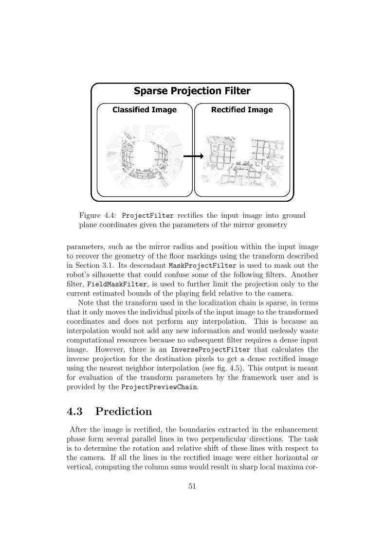
Figure 4.4: ProjectFilter rectifies the input image into groundplane coordinates given the parameters of the mirror geometry

parameters, such as the mirror radius and position within the input imageto recover the geometry of the floor markings using the transform describedin Section 3.1. Its descendant MaskProjectFilter is used to mask out therobot’s silhouette that could confuse some of the following filters. Anotherfilter, FieldMaskFilter, is used to further limit the projection only to thecurrent estimated bounds of the playing field relative to the camera.

Note that the transform used in the localization chain is sparse, in termsthat it only moves the individual pixels of the input image to the transformedcoordinates and does not perform any interpolation. This is because aninterpolation would not add any new information and would uselessly wastecomputational resources because no subsequent filter requires a dense inputimage. However, there is an InverseProjectFilter that calculates theinverse projection for the destination pixels to get a dense rectified imageusing the nearest neighbor interpolation (see fig. 4.5). This output is meantfor evaluation of the transform parameters by the framework user and isprovided by the ProjectPreviewChain.

4.3 Prediction

After the image is rectified, the boundaries extracted in the enhancementphase form several parallel lines in two perpendicular directions. The taskis to determine the rotation and relative shift of these lines with respect tothe camera. If all the lines in the rectified image were either horizontal orvertical, computing the column sums would result in sharp local maxima cor-

51

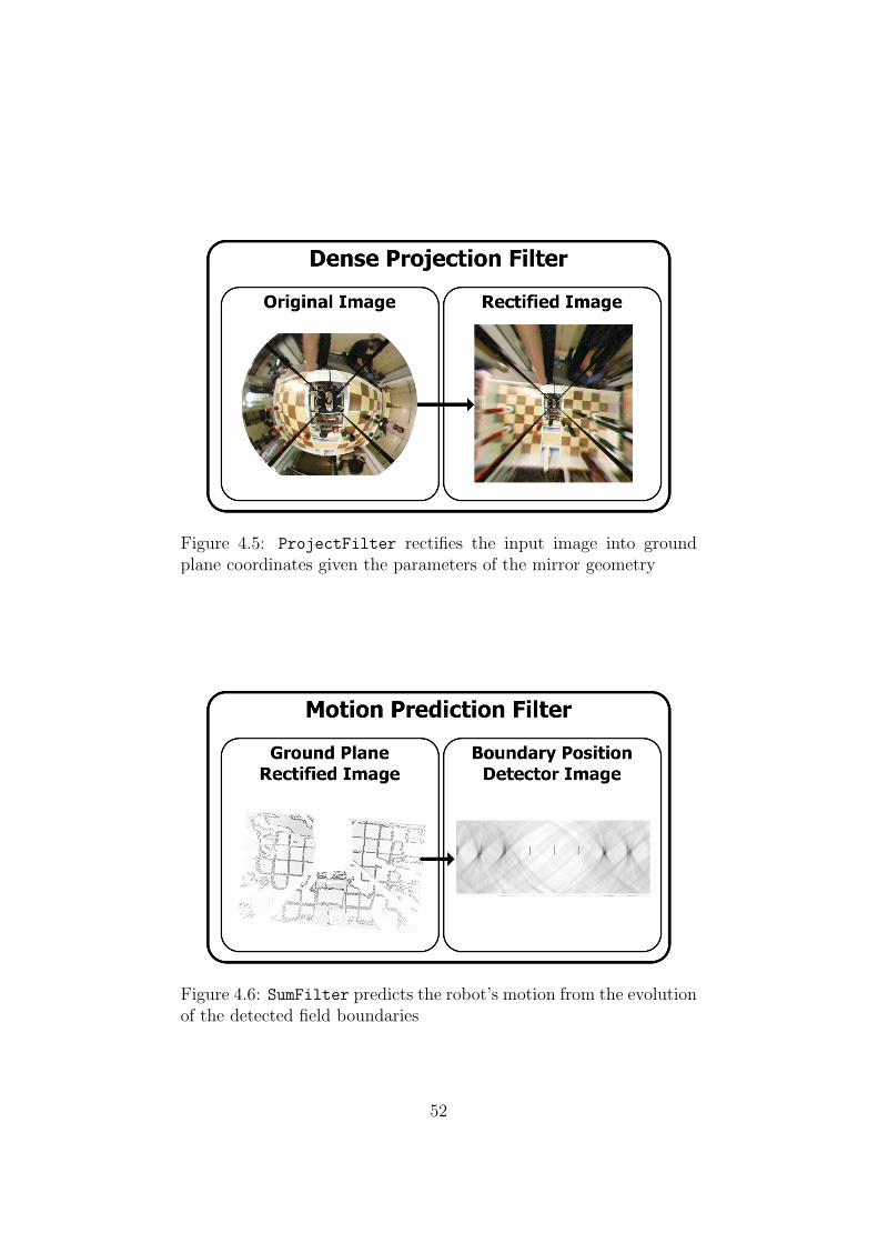
Figure 4.5: ProjectFilter rectifies the input image into groundplane coordinates given the parameters of the mirror geometry

Figure 4.6: SumFilter predicts the robot’s motion from the evolutionof the detected field boundaries

52

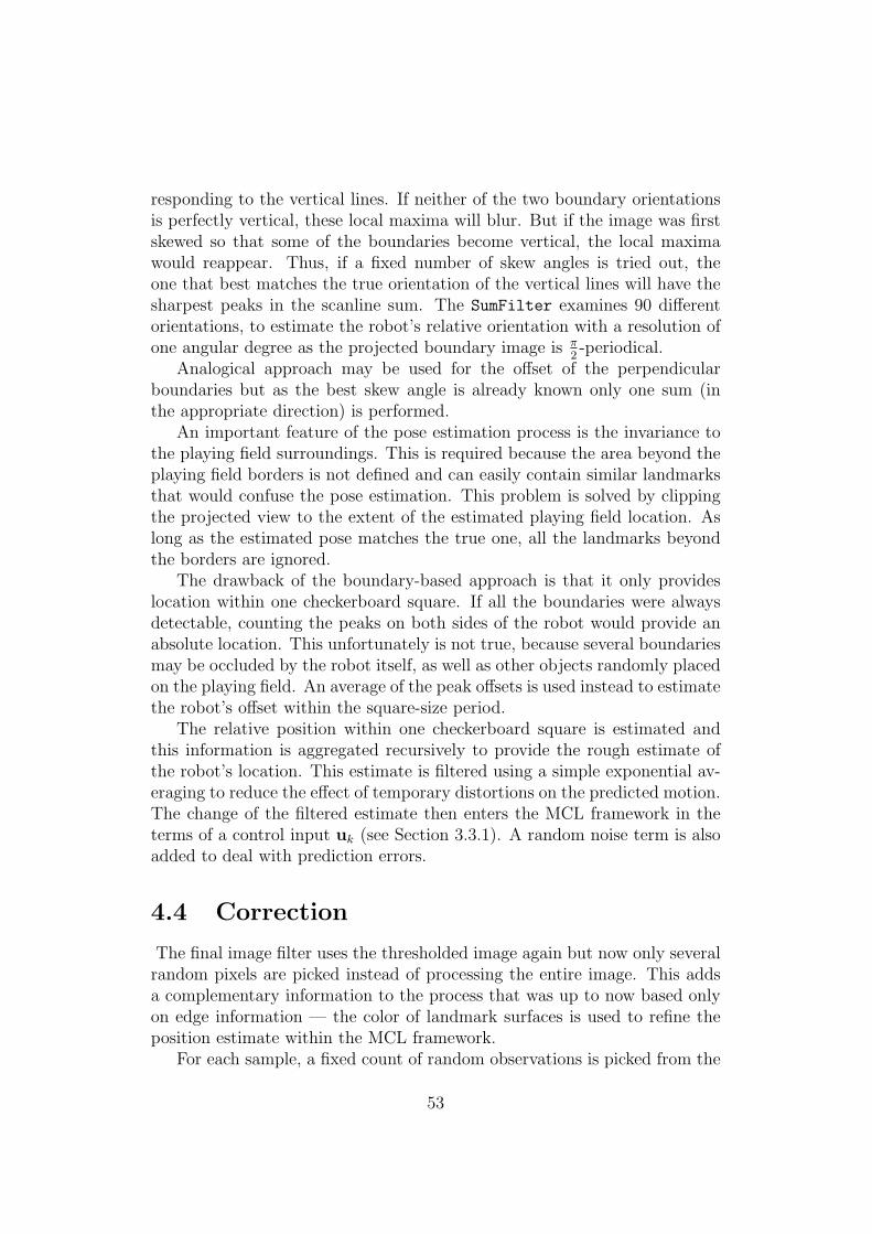
responding to the vertical lines. If neither of the two boundary orientationsis perfectly vertical, these local maxima will blur. But if the image was firstskewed so that some of the boundaries become vertical, the local maximawould reappear. Thus, if a fixed number of skew angles is tried out, theone that best matches the true orientation of the vertical lines will have thesharpest peaks in the scanline sum. The SumFilter examines 90 differentorientations, to estimate the robot’s relative orientation with a resolution ofone angular degree as the projected boundary image is π

2-periodical.

Analogical approach may be used for the offset of the perpendicularboundaries but as the best skew angle is already known only one sum (inthe appropriate direction) is performed.

An important feature of the pose estimation process is the invariance tothe playing field surroundings. This is required because the area beyond theplaying field borders is not defined and can easily contain similar landmarksthat would confuse the pose estimation. This problem is solved by clippingthe projected view to the extent of the estimated playing field location. Aslong as the estimated pose matches the true one, all the landmarks beyondthe borders are ignored.

The drawback of the boundary-based approach is that it only provideslocation within one checkerboard square. If all the boundaries were alwaysdetectable, counting the peaks on both sides of the robot would provide anabsolute location. This unfortunately is not true, because several boundariesmay be occluded by the robot itself, as well as other objects randomly placedon the playing field. An average of the peak offsets is used instead to estimatethe robot’s offset within the square-size period.

The relative position within one checkerboard square is estimated andthis information is aggregated recursively to provide the rough estimate ofthe robot’s location. This estimate is filtered using a simple exponential av-eraging to reduce the effect of temporary distortions on the predicted motion.The change of the filtered estimate then enters the MCL framework in theterms of a control input uk (see Section 3.3.1). A random noise term is alsoadded to deal with prediction errors.

4.4 Correction

The final image filter uses the thresholded image again but now only severalrandom pixels are picked instead of processing the entire image. This addsa complementary information to the process that was up to now based onlyon edge information — the color of landmark surfaces is used to refine theposition estimate within the MCL framework.

For each sample, a fixed count of random observations is picked from the

53

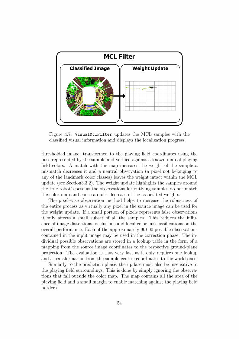
Figure 4.7: VisualMclFilter updates the MCL samples with theclassified visual information and displays the localization progress

thresholded image, transformed to the playing field coordinates using thepose represented by the sample and verified against a known map of playingfield colors. A match with the map increases the weight of the sample amismatch decreases it and a neutral observation (a pixel not belonging toany of the landmark color classes) leaves the weight intact within the MCLupdate (see Section3.3.2). The weight update highlights the samples aroundthe true robot’s pose as the observations for outlying samples do not matchthe color map and cause a quick decrease of the associated weights.

The pixel-wise observation method helps to increase the robustness ofthe entire process as virtually any pixel in the source image can be used forthe weight update. If a small portion of pixels represents false observationsit only affects a small subset of all the samples. This reduces the influ-ence of image distortions, occlusions and local color misclassifications on theoverall performance. Each of the approximately 90 000 possible observationscontained in the input image may be used in the correction phase. The in-dividual possible observations are stored in a lookup table in the form of amapping from the source image coordinates to the respective ground-planeprojection. The evaluation is thus very fast as it only requires one lookupand a transformation from the sample-centric coordinates to the world ones.

Similarly to the prediction phase, the update must also be insensitive tothe playing field surroundings. This is done by simply ignoring the observa-tions that fall outside the color map. The map contains all the area of theplaying field and a small margin to enable matching against the playing fieldborders.

54

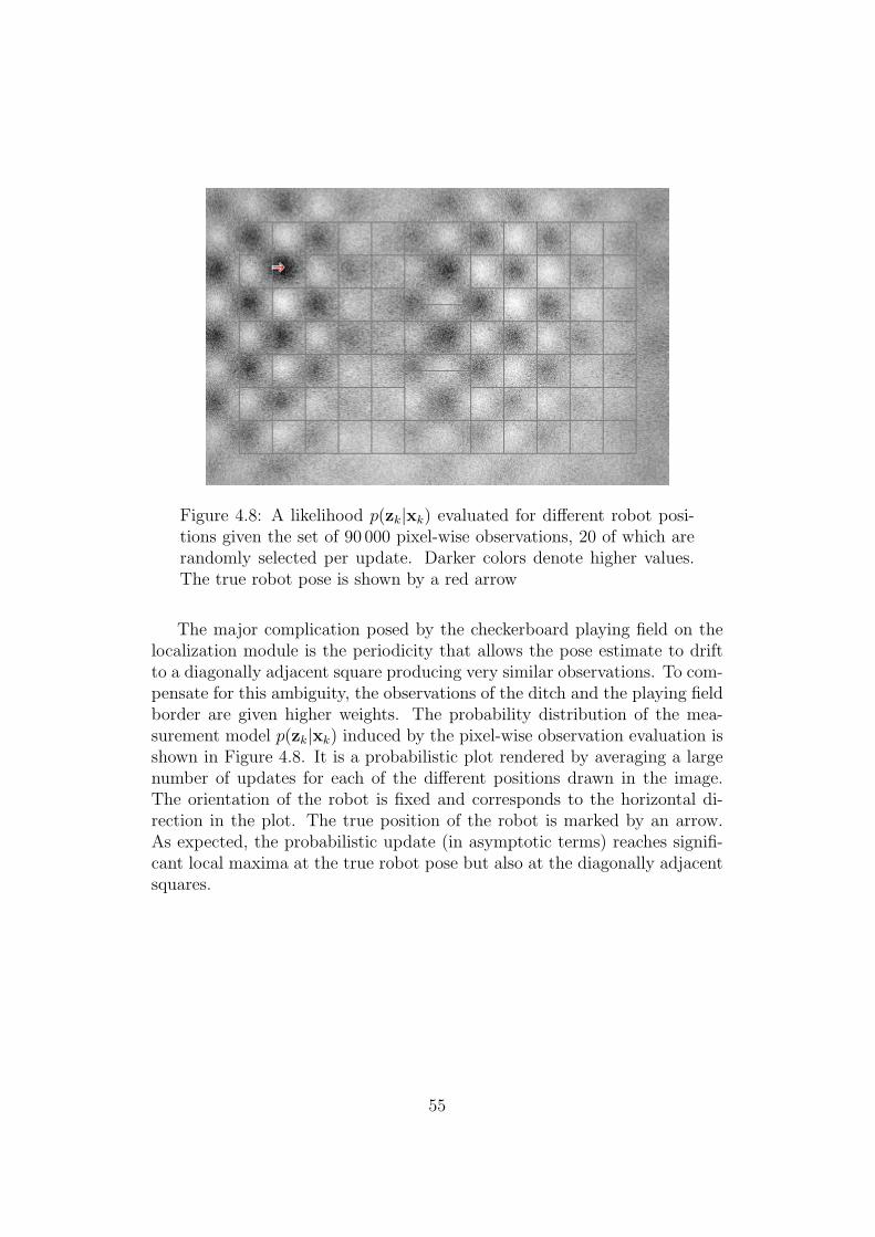
Figure 4.8: A likelihood p(zk|xk) evaluated for different robot posi-tions given the set of 90 000 pixel-wise observations, 20 of which arerandomly selected per update. Darker colors denote higher values.The true robot pose is shown by a red arrow

The major complication posed by the checkerboard playing field on thelocalization module is the periodicity that allows the pose estimate to driftto a diagonally adjacent square producing very similar observations. To com-pensate for this ambiguity, the observations of the ditch and the playing fieldborder are given higher weights. The probability distribution of the mea-surement model p(zk|xk) induced by the pixel-wise observation evaluation isshown in Figure 4.8. It is a probabilistic plot rendered by averaging a largenumber of updates for each of the different positions drawn in the image.The orientation of the robot is fixed and corresponds to the horizontal di-rection in the plot. The true position of the robot is marked by an arrow.As expected, the probabilistic update (in asymptotic terms) reaches signifi-cant local maxima at the true robot pose but also at the diagonally adjacentsquares.

55

Chapter 5

Experiments

To verify the usefulness of the proposed approach, an extensive amount oftests was conducted with the prototype implementation. The experimentswere performed both in simulated conditions and in real-world environment.The results of these two experiment scenarios are given in the following sec-tions. All the experiments were performed off-line, using only the videostream representing an omni-directional view of the operation field.

Ten different sizes of the particle set were always used for the pose estima-tion. All the experiments were repeated several times with 50, 100, 150, 200,250, 300, 400, 500, 750, and 1000 particles to test for the influence of the sizeof the sample set on the accuracy and robustness of the method. Note thatthe computational burden increases linearly depending on the particle counttaking the constant overhead of the image pre-processing into account. Theprocessing speed varied from 20 fps for 50 samples to 13 fps for 1000 sampleson a Celeron-M at 1300MHz.

Fast update rate is important not only for accuracy reasons. The visualodometry also requires that the updates occur frequently enough to resolvethe ambiguity in the motion of the periodic pattern. The maximum for-ward speed must allow two consecutive observations within one checkerboardsquare to determine the direction of the motion. A similar condition appliesto the angular speed. A processing pace of 15 fps imposes an upper bound ofapproximately 2 ms−1 on the forward speed and 4π s−1 on the angular one,which is far enough for a mobile robot acting on a playing field less than 4mlong.

5.1 Simulated Environment

A series of simulated experiments was performed to test the prototype imple-mentation in idealized conditions and to enable evaluation of the maximum

56

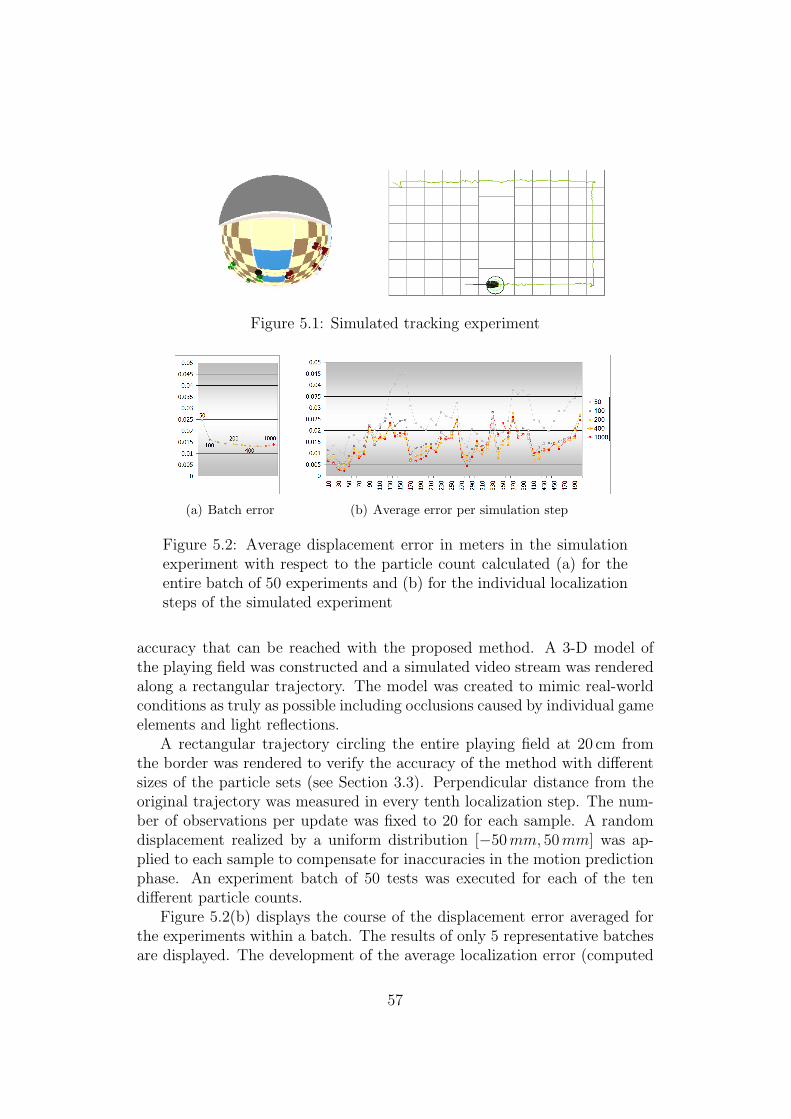
Figure 5.1: Simulated tracking experiment

(a) Batch error (b) Average error per simulation step

Figure 5.2: Average displacement error in meters in the simulationexperiment with respect to the particle count calculated (a) for theentire batch of 50 experiments and (b) for the individual localizationsteps of the simulated experiment

accuracy that can be reached with the proposed method. A 3-D model ofthe playing field was constructed and a simulated video stream was renderedalong a rectangular trajectory. The model was created to mimic real-worldconditions as truly as possible including occlusions caused by individual gameelements and light reflections.

A rectangular trajectory circling the entire playing field at 20 cm fromthe border was rendered to verify the accuracy of the method with differentsizes of the particle sets (see Section 3.3). Perpendicular distance from theoriginal trajectory was measured in every tenth localization step. The num-ber of observations per update was fixed to 20 for each sample. A randomdisplacement realized by a uniform distribution [−50 mm, 50 mm] was ap-plied to each sample to compensate for inaccuracies in the motion predictionphase. An experiment batch of 50 tests was executed for each of the tendifferent particle counts.

Figure 5.2(b) displays the course of the displacement error averaged forthe experiments within a batch. The results of only 5 representative batchesare displayed. The development of the average localization error (computed

57

from all the 2500 localization steps recorded in every batch) is shown in Fig-ure 5.2(a). The displayed value denotes average localization error in meters.The average error falls quickly towards 400 particles. After that it does notdecrease significantly. The best value was reached using 500 particles and itwas approximately 13mm, which is very good.

The biggest local error is reached when passing from one playing fieldside to the other, i.e. when crossing the ditch. It shows up that one smallsimplification can have important influence on the local performance. Theactual simplification included in the localization algorithm is that all thecheckerboard boundaries form a rectangular pattern with a period of 30 cm.In fact, the ditch is separated from the two checkerboards by a 22mm widewhite line, which makes the boundaries detected on the different sides ofthe ditch misaligned by 4.4 cm. This error is unfortunately inherent and isunreplaceable because the motion prediction merges all the detected peaksinto one assuming the 30 cm period. The relative position estimate thusslowly drifts from the coordinate system of one field to the other as theinfluence of the distant boundaries diminishes. In a real-world environmentthis error is negligible compared to other distortions but in the simulatedcase it is noticeable.

As can be seen from the charts the experiments conducted with the simu-lated environment proved that with too small particle sets the localization isnot reliable. Using too many samples is generally not deteriorative althoughtheir update may consume too much computational resources. However, froma certain size the sample set provides a good coverage of the represented PDFand the results do not dramatically improve when adding more samples. Inthis application, the limit particle set contains around 500 particles.

5.2 Target Environment

For the following experiments the original playing field for the Eurobotopen

2005 Czech National Cup [12] was used. The test robotic platform wasequipped with a catadioptric sensor whose hyperbolic mirror was placed45 cm above the ground. Its field-of-view covers the entire operation field.The image was captured using an off-the-shelf web-camera connected to USBand providing thirty 640×480 uncompressed images per second. The robotwas manually pushed along the playing field and the omni-directional videostream was recorded. As noted in Section 2.5, this video stream is sufficientfor the application to be able to reconstruct the original robot’s trajectory.

The prototype application was tested off-line on seven recorded videostreams (see fig.5.4). The average length of a test stream is 40 s, which corre-sponds to 1200 localization steps. The localization process was repeated 70

58

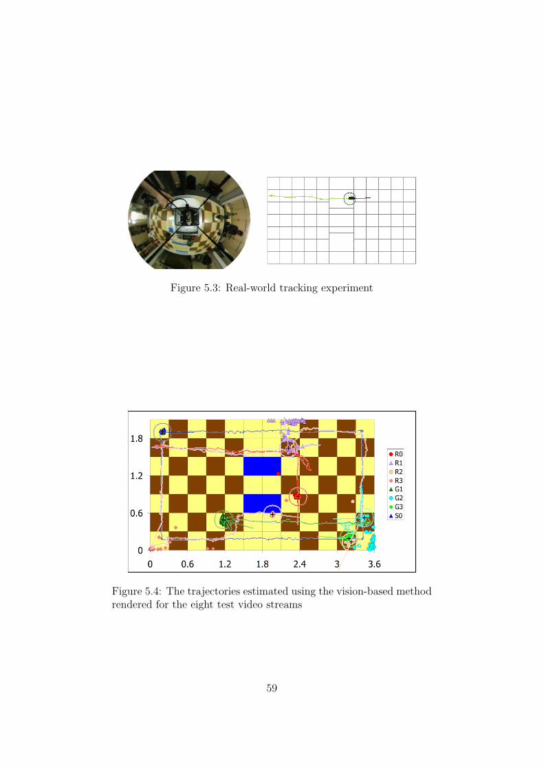
Figure 5.3: Real-world tracking experiment

Figure 5.4: The trajectories estimated using the vision-based methodrendered for the eight test video streams

59

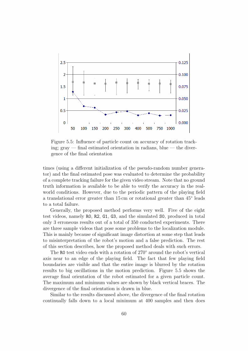
Figure 5.5: Influence of particle count on accuracy of rotation track-ing; gray — final estimated orientation in radians, blue — the diver-gence of the final orientation

times (using a different initialization of the pseudo-random number genera-tor) and the final estimated pose was evaluated to determine the probabilityof a complete tracking failure for the given video stream. Note that no groundtruth information is available to be able to verify the accuracy in the real-world conditions. However, due to the periodic pattern of the playing fielda translational error greater than 15 cm or rotational greater than 45◦ leadsto a total failure.

Generally, the proposed method performs very well. Five of the eighttest videos, namely R0, R2, G1, G3, and the simulated S0, produced in totalonly 3 erroneous results out of a total of 350 conducted experiments. Thereare three sample videos that pose some problems to the localization module.This is mainly because of significant image distortion at some step that leadsto misinterpretation of the robot’s motion and a false prediction. The restof this section describes, how the proposed method deals with such errors.

The R0 test video ends with a rotation of 270◦ around the robot’s verticalaxis near to an edge of the playing field. The fact that few playing fieldboundaries are visible and that the entire image is blurred by the rotationresults to big oscillations in the motion prediction. Figure 5.5 shows theaverage final orientation of the robot estimated for a given particle count.The maximum and minimum values are shown by black vertical braces. Thedivergence of the final orientation is drawn in blue.

Similar to the results discussed above, the divergence of the final rotationcontinually falls down to a local minimum at 400 samples and then does

60

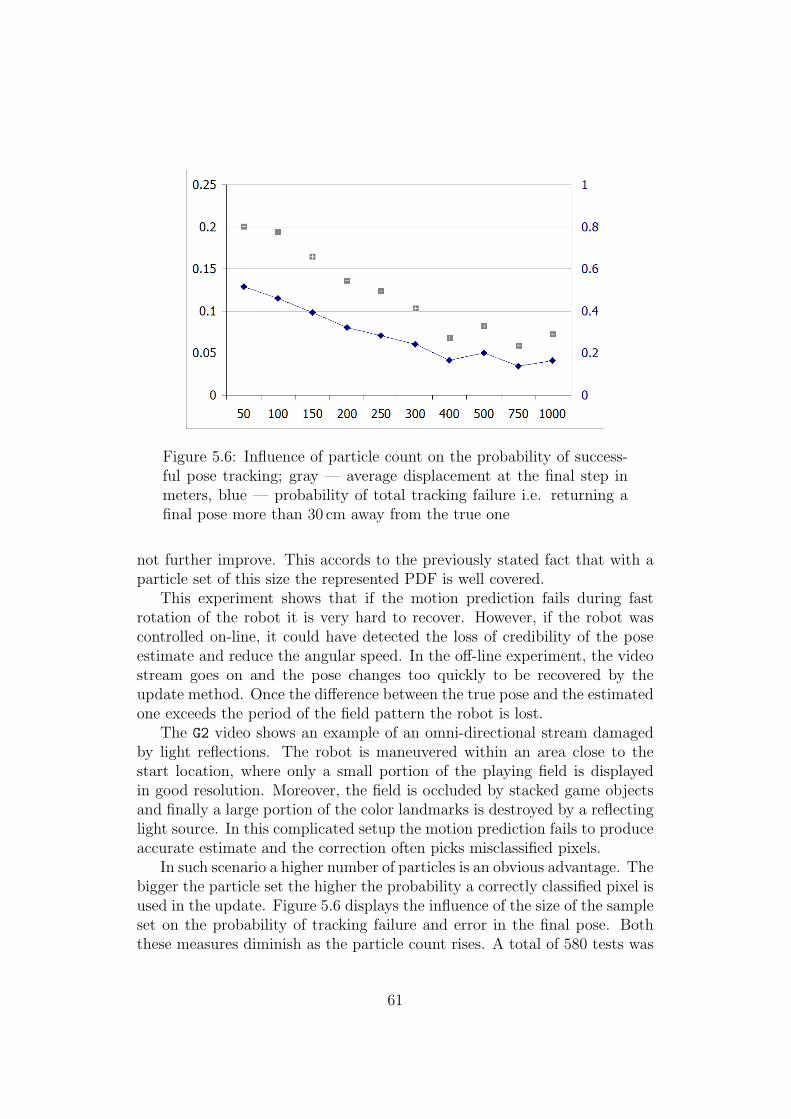
Figure 5.6: Influence of particle count on the probability of success-ful pose tracking; gray — average displacement at the final step inmeters, blue — probability of total tracking failure i.e. returning afinal pose more than 30 cm away from the true one

not further improve. This accords to the previously stated fact that with aparticle set of this size the represented PDF is well covered.

This experiment shows that if the motion prediction fails during fastrotation of the robot it is very hard to recover. However, if the robot wascontrolled on-line, it could have detected the loss of credibility of the poseestimate and reduce the angular speed. In the off-line experiment, the videostream goes on and the pose changes too quickly to be recovered by theupdate method. Once the difference between the true pose and the estimatedone exceeds the period of the field pattern the robot is lost.

The G2 video shows an example of an omni-directional stream damagedby light reflections. The robot is maneuvered within an area close to thestart location, where only a small portion of the playing field is displayedin good resolution. Moreover, the field is occluded by stacked game objectsand finally a large portion of the color landmarks is destroyed by a reflectinglight source. In this complicated setup the motion prediction fails to produceaccurate estimate and the correction often picks misclassified pixels.

In such scenario a higher number of particles is an obvious advantage. Thebigger the particle set the higher the probability a correctly classified pixel isused in the update. Figure 5.6 displays the influence of the size of the sampleset on the probability of tracking failure and error in the final pose. Boththese measures diminish as the particle count rises. A total of 580 tests was

61

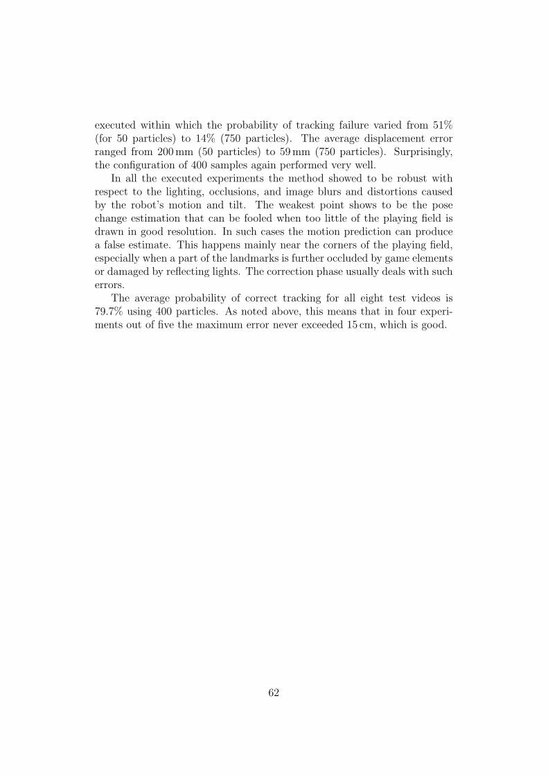
executed within which the probability of tracking failure varied from 51%(for 50 particles) to 14% (750 particles). The average displacement errorranged from 200mm (50 particles) to 59mm (750 particles). Surprisingly,the configuration of 400 samples again performed very well.

In all the executed experiments the method showed to be robust withrespect to the lighting, occlusions, and image blurs and distortions causedby the robot’s motion and tilt. The weakest point shows to be the posechange estimation that can be fooled when too little of the playing field isdrawn in good resolution. In such cases the motion prediction can producea false estimate. This happens mainly near the corners of the playing field,especially when a part of the landmarks is further occluded by game elementsor damaged by reflecting lights. The correction phase usually deals with sucherrors.

The average probability of correct tracking for all eight test videos is79.7% using 400 particles. As noted above, this means that in four experi-ments out of five the maximum error never exceeded 15 cm, which is good.

62

Chapter 6

Conclusion

This work has given a thorough overview of the task of vision-based localiza-tion of a mobile robot within the dynamic environment of a robotic contest.It presented a complete solution that can track a mobile robot anywherewithin the limited contest field using no other than visual sensors, perform-ing real-time visual pose tracking on a general hardware. Since the large fieldof view is important to avoid lack of traceable features in the camera image,a solution using catadioptric omni-directional visual sensor was developed.The method is best suited for localization in a highly dynamic environmentof robotic competitions taking place on delimited operation field painted withan easily detectable color pattern.

6.1 Results

A method for probabilistic ego-motion tracking based on edge and colorfeatures of the playing field reconstructed from an omni-directional imagewas developed. A prototype implementation using Monte Carlo Localizationwas presented and was shown to perform very well in the target environmentof the Eurobotopen 2005 robotic contest. Instead of using an expensive range-finder sensor with ambiguous readings, an affordable combination of an off-the-shelf camera and a hyperbolic mirror was used to produce a reliableposition estimate. The proposed method was able to reconstruct the originalrobot’s trajectory reaching an average accuracy of approximately 15mm. Theresults of both simulated and real-world experiments display the usability ofthe approach and propose several new challenges.

One of the scopes of this work was to evaluate whether a vision-basedodometry that does not suffer from the problem of unmodeled displacementcan completely replace a hardware one. Contrary to the odometry based oncounting the revolutions of wheels that can slip and fail to detect sideways

63

motion caused by collision, the visual odometry detects all the robot’s motionup to a certain speed. This is especially important in situations, where manymoving objects may influence the robot’s intended trajectory. On the otherhand, the visual odometry, as well as the hardware one, produces erroneousmeasurements. The important fact is that the problematic scenarios of thetwo methods do not overlap. A combination of both methods could produceexquisite results.

The major contribution of the work is a new vision-based update methodfor the probabilistic framework that enables to use virtually any pixel of theinput omni-directional image to enhance the pose estimation. The updatemethod only requires a color map of the environment, which is very easy todefine for the playing field of a robotic contest. This new approach decreasesthe influence of local misclassification as different observation items are se-lected for each of the particles. Each of the approximately 90 000 possibleobservations contained in the input image can be used. The evaluation isvery fast, because the observation transforms are pre-calculated.

The important advantage of the omnidirectional sensor is that the imageof entire operation field is available regardless to the robot’s pose. Addition-ally, the evaluation function does not require a specific background beyondthe border of the operation field. The localization process is insensitive tothe surrounding of the playing field, which is not defined.

6.2 Future Research

Further work will focus on merging the hardware odometry information withthe vision-based motion prediction to remove the limitation on the speedof intended motion. Future enhancements may consider a redefinition ofthe motion estimation to enable the method to perform in operation fieldswithout a periodic rectangular pattern.

A global update sensor may also be added to enable relocalizing the robotin case of a tracking failure.

Finally, interesting results could be obtained implementing a feedbackchannel that would affect the robot’s actions depending on the immediatereliability of the estimated pose. The robot can react by reducing speed orperforming actions that may help the localization process to recover usingreliable landmarks.

64

Appendix A

Eurobotopen 2005

This appendix gives additional information on the Eurobotopen 2005 roboticcontest. The complete rules and other documents may be found at [12].

A.1 Rules

Eurobotopen [12] is a competition of amateur teams of young people passion-ate for mobile robotics. To favor participation of new teams and to preventthe more experienced ones from dominating the contest the rules changeevery year.

The theme for 2005 was Bowling. Two robots oppose on the playing fieldtrying to lay down as many skittles as possible. The robots are also allowed toraise up opponnent’s skittles to decrease its score. The match lasts 90 secondsand at the end of the time limit the robots must stop automatically. Thenthe score is counted. The robot with most skittles laying down wins.

A.2 Playing Field

The playing field for the Eurobotopen 2005 contest [12] is a rectangular area3.644m long and 2.1m wide consisting of two fields painted with a brown-beige checkerboard pattern separated by a blue ditch that can be passedusing three bridges (see fig. A.1). Each of the two fields consists of 7×5 tilesmeasuring 30×30 cm. The ditch is 60 cm wide and is separated from the twofields by a white stripe 22mm wide. A white border 7 cm high is encirclingthe playing field. It is assumed to lay outside of the playing field dimensions.

The starting locations of the two robots are in the two opposite corners.The playing field contains following game elements and obstacles, all placedrespecting a central symmetry:

65

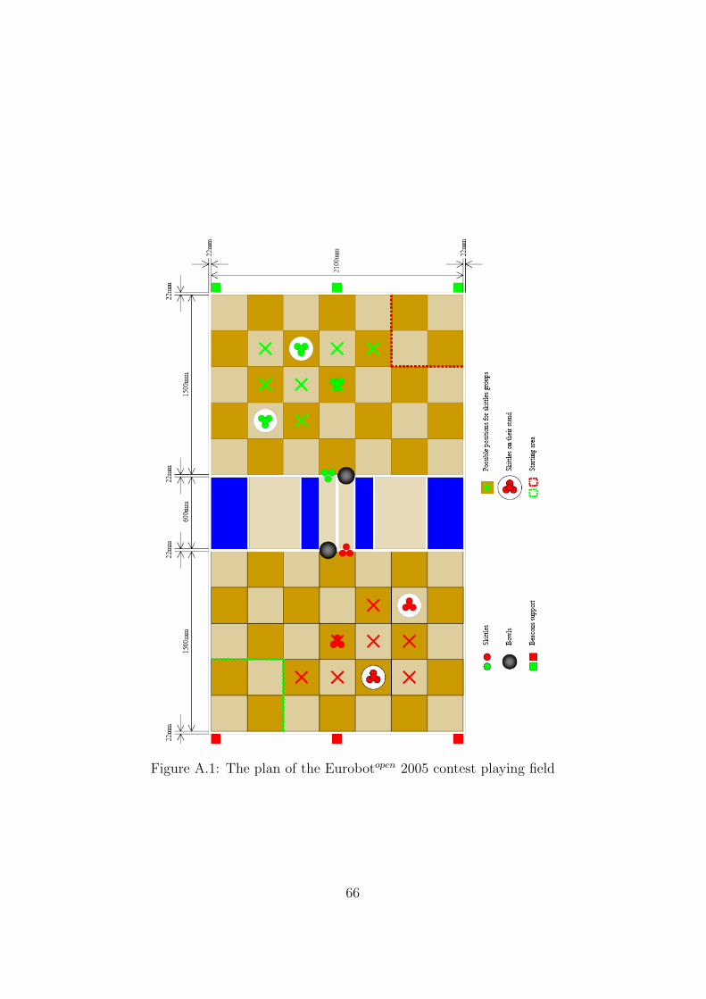
Figure A.1: The plan of the Eurobotopen 2005 contest playing field

66

• 15 green and 15 red skittles (painted wooden cylinders) initially stackedinto 4 piles,

• 4 white skittle stands placed symmetrically under two and two of theskittle piles, and

• 2 black bowls placed on the ends of the central bridge.

67

Appendix B

Target Robotic Platform

The test robotic platform (see fig. B.1) used in the experiments is a differ-entially driven robot with the propelled wheels having 70mm in diametermounted in back and two steerable wheels mounted in the two front corners.The approximate dimensions of the robot are 30×20×32 cm.

The robot is equipped with a web-camera and a hyperbolic mirrormounted 45 cm above ground. The mirror is a hyperbolic glass mirror H3G

from Neovision [38] and is described by the surface equation:

z2

789, 3274− x2 + y2

548, 1440= 1

68

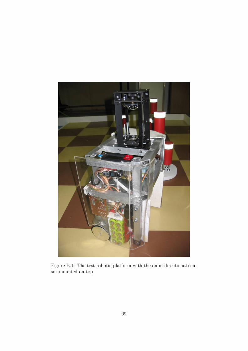
Figure B.1: The test robotic platform with the omni-directional sen-sor mounted on top

69

Appendix C

Attachment CD Contents

The following directories are present on the CD disk:

• bin — Contains all the binaries necessary to run the vision framework.

• bonus — Contains two videos about the Eurobotopencontest.

• OpenCV — Contains a redistribution of the Intel Open Source ComputerVision Library.

• src — Contains the complete source files of the application and aproject file that can be opened with Visual Studio .NET 2003.

• tracking — Contains 9 output videos rendered by the applicationusing the included sample video streams. They are stored both in AVIand QuickTime formats and may be immediately played back.

• vids — Contains 8 sample video streams for the vision framework inthe AVI format.

The directory ‘vids’ contains 8 sample videos that can be used to testthe prototype application. A batch file ‘vision.cmd’ is contained in the ‘vids’directory. It accepts the name of a sample video as the first argument andexecutes the file ‘vision.exe’ in the ‘bin’ directory with the appropriatesettings.

Even simpler, one of the eight batch files in the CD root can be used toexecute the application with one of the sample videos. The following batchfiles are present:

• S0.cmd — Shows a rectangular path rendered in a simulated environ-ment.

• R0.cmd — The robot follows an L-like trajectory across the field.

70

• R1.cmd — The robot goes straight and then rotates by 270◦.

• R2.cmd — The robot goes around the field to the opposite corner.

• R3.cmd — The robot goes close to the start border and passes the farbridge.

• G1.cmd — The robot passes a bridge and turns by 180◦.

• G2.cmd — The robot follows a complicated path near the starting lo-cation.

• G3.cmd — The robot is pulled sideways.

71

Appendix D

Software Documentation

The following sections document the prototype application provided at theattachment CD.

D.1 Vision Framework Usage

Once the vision framework is run (e.g. using one of the batch files in the CDroot) a preview window opens and a list of available commands is printed tothe console. These commands enable viewing different filter chains containedin the framework and to manipulate with the input video. They also enableto save the current chain output to disc.

The commands are as follows:

• 0-5,9 — Selects the displayed filter chain:

• 0 — Preview Chain (displays only the preview of the video)

• 1 — Project Preview Chain (shows the ground-rectified projection)

• 2 — Color Class Edit Chain (displays the color classification)

• 3 — Boundary Detector Chain (shows detected checkerboard bound-aries)

• 4 — Video MCL Chain (displays a pose tracking window)

• 5 — Combined MCL Chain (displays more tracking windows for a de-tailed look onto the localization process; note that the localizationprocess executes if and only if one of this two chains is selected)

• 9 — Threshold Gradient Chain (shows a histogram of the classifiedimage)

72

• SPACE — Pause/Resume (toggles input video playback)

• R — Restarts the input video

• + — Advances 1 s forward in the input video stream

• - — Returns 1 s back in the input video stream

• [ — Skips 1 frame back in the input video stream

• ] — Skips 1 frame forward in the input video stream

• D — Dumps all the current chain images to disk

• C — Capture (continually dumps all windows)

• V — Video (dumps the chain output filter)

• S — Stop capture (stops recording)

• I — Imports the filter settings from disk (implicitly Filters.txt)

• E — Exports the filter settings to disk (implicitly Filters.txt)

• M — Marks (toggles display of calibration marks on the preview image)

• F — Freeze (stops the video stream and counts FPS on the currentframe)

• Q — Query performance (displays the average processing speed)

• x — Exit (the program terminates when the video stream ends)

• ESC — EXIT (the program ends immediately)

Some filters also have interactive windows. These are namely the ‘Pre-view’ window (0: Preview Chain) that enables to change the mirror centerand radius using the middle and right mouse buttons respectively and the‘Colored’ window (2: Color Class Edit Chain) that enables to add andremove pixels to/from the current color class using left mouse button andthe Ctrl/Alt key modifiers respectively.

The ‘VisualMCL’ window of the (5: CombinedMcl Chain) enables to re-place the estimated robot pose using the right mouse button.

Note that the application can be executed directly from the CD. Thebatch files in the CD root can be used to open and test the individual samplevideo streams. When exporting data from the framework, these are storedin the subdirectories of C:/temp/vision.

73

D.2 Description of Vision Framework Files

The directory ‘src’ on the CD contains the following files:

• Capture.h (cpp) — Handles input of the video stream including seeking.

• FilterChain.h — Aggregates the individual filters into chains that canbe executed by the framework.

• Framework.cpp — Main source of the application. Performs handlingof the command-line arguments and interactive commands on chains.

• ImageFilter.h (cpp) — Defines the base class for all the image filters.Handles allocation, reading of settings, output to a window and savingoutput to a file.

• Localize.h (cpp) — Implements the persistent state estimation used inthe tracking.

• MclFilter.h (cpp) — Image filters used for the particle update from theclassified image.

• PreviewFilter.h(cpp) — A set of simple filters that serve for visualiza-tion.

• ProjectFilter.h(cpp) — A set of projection filters that perform the im-age rectification.

• StdAfx.h (cpp) — A precompiled header file.

• SumFilter.h (cpp) — Performs the visual odometry by tracking periodicstraight lines.

• ThresholdFilter.h(cpp) — Classifies the input image using a fast 3Dthresholding.

• Transform.h (cpp) — Implements the mirror reflection transforms usedin the rectification.

• Vision.sln (vcproj) — The project files for the Visual Studio .NET2003.

Note that the project can be opened and compiled from the CD.However, intermediate files as well as the compiled binary are placed inC:/temp/vision. If you want to remove these files later you must do itmanually.

74

The OpenCV library [41] is required for the project to compile. A com-plete package (redistributed under the terms of Intel License Agreement ForOpen Source Computer Vision Library) is included in the OpenCV directory.

The path to the OpenCV library files must be set in the project configu-ration, section Linker|General. It is set to ../OpenCV/lib for the solutionsaved on the CD. If the solution files are moved to other location, this pathmust be reset accordingly.

75

Bibliography

[1] SICK AG. Lms 200 indoor laser measurement system.http://ecatalog.sick.com/Products/ProductFinder/product.aspx?pid=9168.

[2] H. Aihara, N. Iwasa, N. Yokoya, and H. Takemura. Memory-based self-localisation using omnidirectional images. In Proceedings of the 14th Inter-national Conference on Pattern Recognition, pages 297–299. IEEE ComputerSociety Press, Silver Spring, MD, 1998.

[3] H. Andreasson, A. Treptow, and T. Duckett. Localization for mobile robotsusing panoramic vision, local features and particle filter. In Proc. of the ICRA-2005, IEEE International Conference on Robotics & Automation, 2005.

[4] Acroname Articles. Demystifing the Sharp IR rangers.http://www.acroname.com/robotics/info/articles/sharp/sharp.html.

[5] S. Baker and S.K. Nayar. A theory of single-viewpoint catadioptric imageformation. International Journal of Computer Vision, 35(2):1 – 22, 1999.

[6] J. Benda and Z. Winkler. Tracking the absolute position of a mobile robotusing vision-based Monte Carlo Localization. In Proc. of the 1st InternationalConference on Dextrous Autonomous Robots and Humanoids (DARH), 2005.

[7] R.A. Brooks. A robust layered control system for a mobile robot. ArtificialIntelligence at MIT Expanding Frontiers, 2:3–27, 1990.

[8] J. Bruce, T. Balch, and M. Veloso. Fast and inexpensive color image segmen-tation for interactive robots. In Proceedings of the IEEE/RSJ InternationalConference on Intelligent Robots and Systems (IROS), October 2000.

[9] RemoteReality Corporation. Omnialert camera.http://www.remotereality.com/vtprod/oa camera.html.

[10] F. Dellaert, W. Burgard, D. Fox, and S. Thrun. Using the condensation algo-rithm for robust, vision-based mobile robot localization. In Proc. of the IEEEComputer Society Conference on Computer Vision and Pattern Recognition,1999.

[11] G. Dudek and M. Jenkin. Computational principles of mobile robotics. Cam-bridge University Press, New York, NY, USA, 2000.

76

[12] Eurobotopen Competition. Eurobot association. http://eurobot.org/.

[13] The RoboCup Federation. RoboCup official site. http://www.robocup.org/.

[14] D. Fox. Markov Localization: A Probabilistic Framework for Mobile RobotLocalization and Naviagation. PhD thesis, University of Bonn, Germany,1998.

[15] D. Fox, W. Burgard, F. Dellaert, and S. Thrun. Monte Carlo Localization:Efficient position estimation for mobile robots. In AAAI/IAAI, pages 343–349, 1999.

[16] D. Fox, W. Burgard, and S. Thrun. Active markov localization for mobilerobots, 1998.

[17] J. Gaspar, N. Winters, E. Grossmann, and J. Santos-Victor. Toward robotperception using omnidirectional vision. In Innovations in Machine Intelli-gence and Robot Perception, 2004.

[18] H.-M. Gross, A. Koenig, H.-J. Boehme, and Ch. Schroeter. Vision-basedMonte Carlo self-localization for a mobile service robot acting as shoppingassistant in a home store. In Proc. 2002 IEEE/RSJ Int. Conference on In-telligent Robots and Systems (IROS 2002), pages 256–262, 2002.

[19] J.-S. Gutmann and D. Fox. An experimental comparison of localization meth-ods continued. In Proceedings of the IEEE/RSJ International Conference onIntelligent Robots and Systems (IROS’02), 2002.

[20] D. Haehnel, D. Burgard, W. Fox, and Thrun S. An efficient FastSLAMalgorithm for generating maps of large-scale cyclic environments from rawlaser range measurements. In Proceedings of the IEEE/RSJ InternationalConference on Intelligent Robots and Systems (IROS), 2003.

[21] P.V.C. Hough. Machine analysis of bubble chamber pictures. In Proc. of theInternational Conference on High Energy Accelerators and Instrumentation.CERN, 1959.

[22] D. Huttenlocher, R. Lilien, and C. Olsen. View-based recognition using aneigenspace approximation to the hausdorff measure. IEEE Transactions onPattern Analysis and Machine Intelligence, 21(9):951–956, 1999.

[23] Point Grey Research Inc. LadyBug camera.http://www.ptgrey.com/products/ladybug2/index.html.

[24] M. Isard and A. Blake. Condensation conditional density propagation forvisual tracking. International Journal of Computer Vision, 29(1):5–28, 1998.

[25] H. Ishiguro and S. Tsuji. Image-based memory of environment, 1996.

[26] M. Jogan and A. Leonardis. Robust localization using an omnidirectionalappearance-based subspace model of environment. Robotics and AutonomousSystems, Elsevier Science, 45(1):51–72, 2003.

77

[27] R.E. Kalman and R. Bucy. A new approach to linear filtering and predictionproblems. In Trans. ASME, Journal of Basic Engineering, 1960.

[28] David G. Lowe. Distinctive image features from scale-invariant keypoints.International Journal of Computer Vision, 60(2):91–110, 2004.

[29] C. Marques and P. Lima. A localization method for a soccer robot using avision-based omni-directional sensor. RoboCup 2000 Book, 2001.

[30] R. Matousek and L. Zalud. Project Orpheus. http://www.orpheus-project.cz/.

[31] P. Maybeck. Stochastic Models, Estimation and Control, volume Vol. 1. Aca-demic Press, 1979.

[32] E. Menegatti, A. Pretto, and E. Pagello. A new omnidirectional vision sensorfor Monte-Carlo Localization. In Proc. of the 2004 Int. RoboCup SymposiumCD-ROM, 2004.

[33] E. Menegatti, M. Zoccarato, E. Pagello, and H. Ishiguro. Hierarchical image-based localisation for mobile robots with Monte-Carlo Localization. In Proc.of 1st European Conference on Mobile Robots ECMR’03 September 2003,2003.

[34] E. Menegatti, M. Zoccarato, E. Pagello, and H. Ishiguro. Image-based Monte-Carlo Localization with omnidirectional images. Robotics and AutonomousSystems, Elsevier Volume 48, Issue 1, pages 17–30, 2004.

[35] H. P. Moravec. The stanford cart and the cmu rover. IEEE, 71(7):872–884,1983.

[36] A. Motomura, T. Matsuoka, and T. Hasegawa. Self-localization method usingtwo landmarks and dead reckoning for autonomous mobile soccer robots. InRoboCup 2003, pages 526–533, 2003.

[37] National Oceanic National Geodetic Survey and Atmospheric Ad-ministration (NOAA). Removal of GPS selective availability.http://www.ngs.noaa.gov/FGCS/info/sans SA/.

[38] Neovision. H3S hyperbolic mirror. http://neovision.cz/prods/panoramic/h3s.html.

[39] T. Pajdla and V. Hlavac. Image-based self-localization by means of zero phaserepresentation in panoramic images. In In Proceedings of the 2nd Interna-tional Conference on Advanced Pattern Recognition volume 2013 of LectureNotes in Computer Science, pages 24–33, 2003.

[40] L. Paletta, S. Frintrop, and J. Hertzberg. Robust localization using contextin omnidirectional imaging. In Proc. ICRA 2001, pages 2072–2077, 2001.

[41] Intel Research. Open source computer vision library.http://www.intel.com/research/mrl/research/opencv/.

78

[42] D. Sekimori, T. Usui, Y. Masutani, and F. Miyazaki. High-speed obstacleavoidance and self-localization for mobile robots based on omni-directionalimaging of floor region. In RoboCup 2001: Robot Soccer World Cup V, pages204–213, London, UK, 2002. Springer-Verlag.

[43] D. Sekimori, T. Usui, Y. Masutani, and F. Miyazaki. Evaluation of self-localization performance for a local vision robot in the small size league. InLecture Notes in Computer Science, volume 2752, pages 41–52, 2003.

[44] R. Sim, P. Elinas, M. Griffin, and J.J. Little. Vision-based SLAM usingthe rao-blackwellised particle filter. In IJCAI Workshop on Reasoning withUncertainty in Robotics (RUR), 2005.

[45] R. Sim, M. Griffin, A. Shyr, and J.J. Little. Scalable real-time vision-basedSLAM for planetary rovers. In Proceedings of the IEEE IROS Workshop onRobot Vision for Space Applications, 2005.

[46] R. Simmons and S. Koenig. Probabilistic robot navigation in partially ob-servable environments. In Proc. of the International Joint Conference onArtificial Intelligence, pages 674–679, 1995.

[47] J. Sladek. Detekce orientacnıch bodu pro mobiln roboty. Master’s thesis,Charles University in Prague, Faculty of Mathematics and Physics, 2003.

[48] A.F.M. Smith and A.E. Gelfand. Bayesian statistics without tears: Asampling-resampling perspective. American Statistician, 46(2):84–88, 1992.

[49] S. Thrun, D. Fox, W. Burgard, and F. Dellaert. Robust Monte Carlo Local-ization for mobile robots. Artificial Intelligence, 128(1-2):99–141, 2001.

[50] J.W. Weingarten, G. Gruener, and R. Siegwart. A state-of-the-art 3d sensorfor robot navigation. In Proceedings of the IEEE/RSJ International Confer-ence on Intelligent Robots and Systems (IROS), 2004.

[51] J. Wolf and A. Pinz. Particle filter for self localization using panoramic vision.OGAI Journal, 22(4):8–15, March 2003.

[52] Y. Yagi, Y. Nishizawa, and M. Yachida. Map-based navigation for a mobilerobot with omnidirectional image sensor copis. IEEE Trans. Robotics andAutomation, 11(5):634–648, 1995.

79