navigation functionalities for an autonomous uav · pdf file ·...
TRANSCRIPT

Linkoping Studies in Science and Technology
Thesis No. 1307
Navigation Functionalities for anAutonomous UAV Helicopter
by
Gianpaolo Conte
Submitted to Linkoping Institute of Technology at Linkoping University in partialfulfillment of the requirements for degree of Licentiate of Engineering
Department of Computer and Information ScienceLinkoping universitet
SE-581 83 Linkoping, Sweden
Linkoping 2007


Navigation Functionalities for anAutonomous UAV Helicopter
by
Gianpaolo Conte
March 2007ISBN 978-91-85715-35-0
Linkoping Studies in Science and TechnologyThesis No. 1307ISSN 0280-7971
LiU-Tek-Lic-2007:16
ABSTRACT
This thesis was written during the WITAS UAV Project where one of the goals has
been the development of a software/hardware architecture for an unmanned autonomoushelicopter, in addition to autonomous functionalities required for complex mission sce-
narios. The algorithms developed here have been tested on an unmanned helicopter
platform developed by Yamaha Motor Company called the RMAX.The character of the thesis is primarily experimental and it should be viewed as
developing navigational functionality to support autonomous flight during complex real-
world mission scenarios. This task is multidisciplinary since it requires competence inaeronautics, computer science and electronics.
The focus of the thesis has been on the development of a control method to enablethe helicopter to follow 3D paths. Additionally, a helicopter simulation tool has been
developed in order to test the control system before flight-tests. The thesis also presents
an implementation and experimental evaluation of a sensor fusion technique based on aKalman filter applied to a vision based autonomous landing problem. Extensive exper-
imental flight-test results are presented.
The work in this thesis is supported in part by grants from the Wallenberg Founda-
tion, the SSF MOVIII strategic center and an NFFP04-031 ”Autonomous flight controland decision making capabilities for Mini-UAVs” project grant.
Department of Computer and Information ScienceLinkoping universitet
SE-581 83 Linkoping, Sweden


v
Acknowledgements
This work would have not been possible without the support and help ofmy family, colleagues and friends. I would like to thanks all of them here.
Especially I would like to thanks:
My supervisor Patrick Doherty who has believed in me supporting myresearch and helping me in the time of darkness.
Simone Duranti for too many things: for the exciting and productivediscussions about (but not only) UAVs, for his intuitions and many inputsto my research and for sharing a common point of view on the definitionof ”good food”.
My colleagues Piotr Rudol, Fredrik Heintz, Per-Magnus Olsson, SimoneDuranti and Per Nyblom to have spent part of their time to go through mythesis and giving me vital feedback.
Piotr and Mariusz for their effort, time and especially extra time putinto the project, for making the robot-lab never boring and for keeping therobot-lab fridge never empty on friday.
All the AIICS members for being available at anytime and for makingthe working environment always friendly.
Felix and Dave with whom I share the hard task of surviving the Swedishwinter, I have to say they make it so much easier.
I also thanks the swedish authority for all the presents left under thewindshield wipers of my car, especially for not enforcing to pay them.
My family and Roberta for being there.


Preface
”To fly is my religion.”Richard Bach
To Antonio.
The work presented in this thesis was done as part of the requirement fora Licentiate degree at the Artificial Intelligence and Integrated ComputerSystem (AIICS) division at Linkoping University. The focus of the thesishas been on development of navigation functionalities for an unmannedhelicopter. A flight control mode which enables an unmanned helicopterto follow 3D paths has been developed (Paper I, Paper II). Additionally,a sensor fusion technique has been applied to a vision based autonomouslanding problem (Paper III).
The original refereed and published papers upon which this thesis isbased are included as an appendix to this thesis:
Paper I G. Conte, S. Duranti, T. Merz. Dynamic 3D Path Followingfor an Autonomous Helicopter. Proc. of the IFAC Symposium onIntelligent Autonomous Vehicles, 2004.
Paper II M. Wzorek, G. Conte, P. Rudol, T. Merz, S. Duranti, P. Do-herty. From Motion Planning to Control - A Navigation Frameworkfor an Autonomous Unmanned Aerial Vehicle. 21th Bristol UAV Sys-tems Conference, 2006.
Paper III T. Merz, S. Duranti, and G. Conte. Autonomous landing ofan unmanned aerial helicopter based on vision and inertial sensing.Proc. of the 9th International Symposium on Experimental Robotics,2004.
Linkoping, January 2007
Gianpaolo Conte


ix
Contents
1 Introduction 1
2 Overview 52.1 UAV software architecture . . . . . . . . . . . . . . . . . . . 52.2 The UAV helicopter platform . . . . . . . . . . . . . . . . . 8
3 Simulation 133.1 Introduction . . . . . . . . . . . . . . . . . . . . . . . . . . . 133.2 Hardware-in-the-loop simulation . . . . . . . . . . . . . . . 143.3 Reference frames . . . . . . . . . . . . . . . . . . . . . . . . 173.4 The augmented RMAX dynamic model . . . . . . . . . . . 19
3.4.1 Augmented helicopter attitude dynamics . . . . . . . 193.4.2 Helicopter equations of motion . . . . . . . . . . . . 20
3.5 Simulation results . . . . . . . . . . . . . . . . . . . . . . . 233.6 Conclusion . . . . . . . . . . . . . . . . . . . . . . . . . . . 28
4 Path Following Control Mode 294.1 Introduction . . . . . . . . . . . . . . . . . . . . . . . . . . . 294.2 Trajectory generator . . . . . . . . . . . . . . . . . . . . . . 31
4.2.1 Calculation of the path geometry . . . . . . . . . . . 324.2.2 Feedback method . . . . . . . . . . . . . . . . . . . . 354.2.3 Outer loop reference inputs . . . . . . . . . . . . . . 37
PFCM kinematic constraints . . . . . . . . . . . . . 37Calculation of the outer loop inputs . . . . . . . . . 41

x CONTENTS
4.3 Outer loop control equations . . . . . . . . . . . . . . . . . 494.4 Experimental results . . . . . . . . . . . . . . . . . . . . . . 504.5 Conclusions . . . . . . . . . . . . . . . . . . . . . . . . . . . 53
5 Sensor fusion for vision based landing 575.1 Filter architecture . . . . . . . . . . . . . . . . . . . . . . . 61
5.1.1 Filter initialization . . . . . . . . . . . . . . . . . . . 615.1.2 INS mechanization . . . . . . . . . . . . . . . . . . . 625.1.3 Kalman filter . . . . . . . . . . . . . . . . . . . . . . 62
5.2 Experimental results . . . . . . . . . . . . . . . . . . . . . . 645.3 Conclusion . . . . . . . . . . . . . . . . . . . . . . . . . . . 71
A 75A.1 Paper I . . . . . . . . . . . . . . . . . . . . . . . . . . . . . 76A.2 Paper II . . . . . . . . . . . . . . . . . . . . . . . . . . . . . 82A.3 Paper III . . . . . . . . . . . . . . . . . . . . . . . . . . . . 97
1
Chapter 1
Introduction
An Unmanned Aerial Vehicle (UAV) is an aerial vehicle without a hu-man pilot on board. It can be autonomous, semi-autonomous or radio-controlled. In the past, the use of UAVs have been mostly related to mili-tary applications in order to perform the so-called Dirty, Dull and Danger-ous (D3) missions such as reconnaissance, surveillance and location acqui-sition of enemy targets. Recently, interest for UAV systems has grown inthe direction of civil applications as a consequence of the cost reduction ofthis technology.
Aircraft navigation can be accomplished by safely solving four tasks:decision making, obstacle perception, aircraft state estimation (estimationof position, velocity and attitude) and aircraft control. In the earlier daysof aeronautic history, the on-board pilot had to solve these tasks by usinghis own skills. Nowadays the situation is quite different since a high levelof automation is present in modern military and civil aircrafts. In orderto replace the pilot completely a number of problems have to be solved.For example, it is difficult to replace the skills of a pilot in perceiving andavoiding obstacles. This is one of the reasons why the introduction of UAVsin non-segregated airspace still represents a challenge.
The work presented in this thesis was initiated as part of the WITASUAV Project [17, 2], where the main goal was to develop technologiesand functionalities necessary for the successful deployment of a fully au-
2 CHAPTER 1. INTRODUCTION
tonomous Vertical Take Off and Landing (VTOL) UAV. The typical op-erational environment for this research has been urban areas where anautonomous helicopter can be deployed for missions such as traffic moni-toring, photogrammetry, surveillance, etc.
Many universities [26, 28, 1, 19, 10, 27, 29] have been and continue todo research with autonomous helicopter systems. Most of the research hasfocused on low-level control of such systems with less emphasis on high-autonomy as in the WITAS UAV Project.
To accomplish complex autonomous missions, high-level functionalitiessuch as mission planning and real world scene understanding have to beintegrated with low-level functionalities such as motion control, sensingand control mode coordination. Details and discussions relative to theWITAS UAV software architecture can be found in [3, 15].
This thesis focuses on two aspects of the navigation task: flight controland state estimation. The main results of this thesis have been publishedin Paper I and Paper II (see Appendix) which are related to flight controlissues, and Paper III (see Appendix) related to sensor fusion and state esti-mation applied to the problem of a vision based autonomous landing. Thealgorithms presented are implemented and tested on a UAV helicopter andcurrently in use in the context of a number of autonomous UAV missions.
The thesis also presents a simulation tool developed for control systemvalidation. The simulator is based on system identification work describedin [4]. The helicopter simulator has been an invaluable tool for developmentof flight control modes. It is implemented in the C-language and coupled tothe complete software architecture. Simulation tests can be done in real-time and with actual helicopter hardware-in-the-loop. A complete flightmission can be tested in the field with the helicopter hardware in-the-loopbefore the actual flight test.
The first contribution of this thesis (Paper I) is the development of aPath Following Control Mode (PFCM). This control mode enables the UAVhelicopter to follow 3D geometric paths. A basic functionality required fora UAV is the ability to fly from a starting location to a goal location. Asstated before, in order to achieve this task safely the helicopter must per-ceive and than avoid eventual obstacles on its way. Additionally, it muststay within the allowed flight control envelope. The UAV developed duringthe WITAS UAV Project has the capability of using a priori knowledge
3
of the environment in order to avoid static obstacles. An on-board pathplanner uses this knowledge to generate collision-free paths. Details of thepath planning methods used are in [18]. The PFCM presented in this the-sis, together with the path execution mechanism, gives the right balancebetween safety and flexibility and can also be used for dynamic path plan-ning. Recently some experiments have been made to exploit the possibilityof avoiding no-fly-zones which are added dynamically from a ground con-trol station or other sources during flight. These experiments are intendedto provide more dynamic path planning. Details of these experiments areavailable in [30]. A natural extension of this feature is the replacement ofthe manual selection of no-fly-zones with an automatic selection. Providedthe UAV has the capability to detect obstacles in the environment, thesecan be treated as no-fly-zones and avoided by using the existing dynamicpath planning capability.
Paper II contains an extended description of the WITAS UAV naviga-tion framework and it shows how the PFCM is integrated in the softwarearchitecture and used in complex missions.
The second contribution of the thesis is the integration of a KalmanFilter (KF) into the control system architecture. The KF is used to fusethe information coming from different sensors available on-board the UAVin order to estimate the helicopter state. The estimated state is used by thecontrol system to control the helicopter. The reason why several sensorsare fused together is because each sensor has different properties whichshould be taken advantage of. In this thesis the KF is used for fusinginertial sensors (INS) and a vision sensor for the vision based autonomouslanding problem described in Paper III. The same KF is implemented onthe UAV helicopter for fusing GPS together with inertial sensors. The reuseof software for different applications is highly desirable in such a complexsystem such as an autonomous UAV.
Vision based autonomous landing is a challenging problem. Landing isthe most dangerous phase of a flight, so the state estimation of a UAV mustbe accurate and continuous in time. The autonomous landing problem issolved by using high accuracy position data from a vision system which usesa single camera and inertial data taken from an Inertial Measurement Unit(IMU). What makes this application special is the fact that the GPS is notused at all during autonomous landing. This makes the UAV independent

4 CHAPTER 1. INTRODUCTION
of external position signals.The UAV platform used for the experimentation is an RMAX unmanned
helicopter manufactured by Yamaha Motor Company. The hardware andsoftware necessary for autonomous flight have been developed during theWITAS UAV Project using off -the-shelf hardware components.
Flight missions are performed in a training area of approximately onesquare kilometer in the south of Sweden, called Revinge (Fig.1.1). The areais used mainly for fire fighter training and includes a number of buildingstructures and road network. An accurate 3D model of the area is availableon board the helicopter in a GIS (Geographic Information System), whichis used for mission planning purposes.
Figure 1.1: Orthophoto of the flight-test area in Revinge (south of Sweden).
5
Chapter 2
Overview
This chapter presents an overview of the UAV architecture developed dur-ing the WITAS UAV Project. The components which have been developedand are part of this thesis will be considered in this context.
A description of the UAV helicopter platform used for the experimentaltests will also be presented. Details of the platform which are relevant tothis thesis will also be considered in order to gain a better understandingof the components developed.
2.1 UAV software architecture
The software architecture developed during the WITAS UAV Project is acomplex distributed architecture for high level autonomous missions. Thearchitecture enables the UAV to perform so-called push button mission.This is intended to mean that a UAV is capable of planning and executinga mission from take-off to landing with limited, or no human intervention.An example of such a mission demonstrated in an actual flight experimentis a photogrammetry scenario. In such a scenario a UAV helicopter isgiven the task of taking pictures of each of the facades of a selected setof buildings input by a ground operator. The details of this mission aredescribed in Paper II. To accomplish this kind of mission, an architecture

6 CHAPTER 2. OVERVIEW
which integrates many different functionalities is required.Fig. 2.1 provides a schematic of the software architecture that has been
developed. The modules focused on in this thesis have been emphasizedin the schematic. The boxes emphasized with bold lines and text havebeen developed and made operational and will be described in detail inthis thesis.
Figure 2.1: UAV software architecture schematic. The modules emphasizedusing bold lines are the focus of this thesis.
The software architecture has been implemented using three computers
2.1. UAV SOFTWARE ARCHITECTURE 7
which will be described shortly.
• The deliberative/reactive system (DRC) executes a number of highlevel functionalities of a deliberative nature such as path planner,execution monitoring, GIS, etc.
• The image processing system (IPC) executes image processing func-tions and handles everything which is related to the video camera(frame grabbing, camera pan/tilt control, etc.).
• The primary flight control system (PFC) executes the control modes(hovering, path following, take-off, landing, etc.), the sensor fusionfunctions (INS/GPS, INS/camera) and handles communication withthe helicopter platform and with the other sensors (GPS, pressuresensor, etc.).
The PFC executes predominantly hard real-time tasks such as the flightcontrol modes or the sensor fusion algorithms. This part of the system usesa Real-Time Application Interface (RTAI) [14] which provides industrial-grade real-time operating system functionality. RTAI is a hard real-timeextension to a standard Linux kernel (Debian) and has been developed atthe Department of Aerospace Engineering of Politecnico di Milano. TheDRC has reduced timing requirements. This part of the system uses theCommon Object Request Broker Architecture (CORBA) as its distribu-tion backbone. Currently an open source implementation of CORBA 2.6called TAO/ACE [11] is in use. More details about the complete softwarearchitecture can be found in Paper III and in [3, 15].
As can be observed from the boxes emphasized in Fig. 2.1, this thesisdeals with a number of functionalities which are contained in the PFCsystem. A brief introduction as to what these functionalities actually dowill now be described.
The simulator mentioned in the introduction implements the helicopterdynamics. Moreover it emulates the helicopter sensor outputs so that dur-ing the simulation the complete software architecture can be tested in aclosed loop. The simulator can also run on the on board hardware so thatduring the simulation it is possible to see the helicopter actuators movingas they would in actual flight. Such simulation using hardware-in-the-loop

8 CHAPTER 2. OVERVIEW
provides a powerful way to quickly test the correct functioning of all thecomponents on the field, including the interface to the helicopter.
The path following control mode (PFCM) enables the helicopter tofollow a 3D path. It receives a geometric description of a path via a numberof parameters from the path planner. From these parameters it generatesa continuous description of the path, then it adds velocity and accelerationconstraints in order to calculate the inputs to be sent to the helicopter. Analgorithm which generates the proper control inputs at each control cyclehas been developed. The PFCM also generates a number of events andother outputs which are necessary for monitoring purposes in flight.
The two sensor fusion algorithms implemented are based on a Kalmanfilter and produce estimates of the helicopter state in terms of position, ve-locity and attitude. They are used to fuse the inertial sensors with the GPS,and the inertial sensors with the video camera during autonomous landing.Since they are based on the same dynamic model, only the results of theintegration between inertial sensors and video camera will be presented. Itwill be shown how the integration of the video camera with inertial sen-sors can effectively improve the robustness of the helicopter state estimatecompared to a solution obtained from image processing alone.
2.2 The UAV helicopter platform
The Yamaha RMAX helicopter used for the experimentation (Fig. 2.2) hasa total length of 3.6 m (including main rotor). It is powered by a 21 hptwo-stroke engine and has a maximum takeoff weight of 95 kg.
The RMAX rotor head is equipped with a Bell-Hiller stabilizer bar(see Fig.2.3). The effect of the Bell-Hiller mechanism is to reduce theresponse of the helicopter to wind gusts. Moreover, the stabilizer bar isused to generate a control augmentation to the main rotor cyclic input.The Bell-Hiller mechanism is very common in small-scale helicopters butquite uncommon in full-scale helicopters. The reason for this is that asmall-scale helicopter experiences less rotor-induced damping compared tofull-scale helicopters. Consequently, it is more difficult to control for ahuman pilot. It should be pointed out though that an electronic controlsystem can stabilize a small-scale helicopter without a stabilizer bar quite

2.2. THE UAV HELICOPTER PLATFORM 9
Figure 2.2: The RMAX helicopter.
efficiently. For this reason the trend for small-scale autonomous helicoptersis to remove the stabilizer bar and let the digital control system stabilize thehelicopter. The advantage in this case is reduced mechanical complexity inthe system.
Figure 2.3: The RMAX rotor head with Bell-Hiller mechanism.

10 CHAPTER 2. OVERVIEW
The RMAX helicopter has a built-in attitude sensor called YAS (YamahaAttitude Sensor) composed of three accelerometers and three rate gyros.The output of the YAS are acceleration and angular rate on the three he-licopter body axes (see section 3.3 for a definition of body axis). The YASalso computes the helicopter attitude angles. Acceleration and angularrate from the YAS will be used as inertial measurement data for the sensorfusion process which will be described in chapter 5.
The RMAX also has a built-in digital attitude control system calledYACS (Yamaha Attitude Control System). The YACS stabilizes the heli-copter attitude dynamics and the vertical channel dynamics. The YACS isused in all the helicopter control modes as an attitude stabilization system.
The hardware platform developed during the WITAS UAV Project isintegrated with the Yamaha platform as shown in Fig. 2.4. It is based onthree PC104 embedded computers.
DRC - 1.4 GHz P-M - 1GB RAM - 512 MB flash
IPC - 700 MHz PIII - 256MB RAM - 512 MB flash
Yamaha RMAX (YAS, YACS)
ethernetswitch
PFC - 700 MHz PIII - 256MB RAM - 512 MB flash
sensor suite
sensorsuite
RS232C Ethernet Other media
Figure 2.4: On-board hardware schematic.
2.2. THE UAV HELICOPTER PLATFORM 11
The PFC is implemented on a 700Mhz Pentium III and includes a wire-less Ethernet bridge, a GPS receiver and a barometric altitude sensor. Anearlier version of the system included a compass as a heading sensor source.The compass has been removed from the latest version since the Kalmanfilter which fuses the inertial sensors and GPS provides sufficiently stableheading information. The PFC communicates with the helicopter througha serial line RS232C, where the inertial sensor data from the YAS is passedto the PFC. The PFC can also send control inputs to the YACS for he-licopter control. The IPC runs on a second PC104 embedded computer(PIII 700MHz), and includes a color CCD camera mounted on a pan/tiltunit, a video transmitter and a video recorder (miniDV). The DRC systemruns on the third PC104 embedded computer (Pentium-M 1.4GHz) andexecutes all high-end autonomous functionality. Network communicationbetween computers is physically realized with serial line RS232C and Eth-ernet. Ethernet is mainly used for CORBA applications, remote login andfile transfer, while serial lines are used for hard real-time networking.

12 CHAPTER 2. OVERVIEW

13
Chapter 3
Simulation
3.1 Introduction
This chapter describes the simulation tool which has been used to developand test the control system for the RMAX helicopter. It is used to test thehelicopter missions both in the lab and on the field. The RMAX helicoptersimulator is implemented in the C language and allows testing of all thecontrol modes developed. Many flight-test hours have been avoided dueto the possibility of running, in simulation, the exact code of the controlsystem which is executed on the on-board computer during the actual flight-test.
In order to develop and test the helicopter control system a mathe-matical model which represents the dynamic behavior of the helicopteris required. The simulator described in this section is specialized for theYamaha RMAX helicopter in the sense that the model includes the dy-namics of the bare platform in addition to the Yamaha Attitude ControlSystem (YACS).
The YACS system stabilizes the pitch and roll angles of the helicopter,the yaw rate and the vertical velocity. The reason why the YACS has beenused was to speed up the control development process and to shift thefocus toward development of functionalities such as the PFCM presented

14 CHAPTER 3. SIMULATION
in chapter 4. All of the currently developed flight modes use the YACS as aninner control loop which stabilizes the high frequency helicopter dynamics.Experimental tests have shown that the YACS decouples the helicopterdynamics so that the pitch, roll, yaw and vertical channels can be treatedseparately in the control system design. In other words the channels donot influence each other.
3.2 Hardware-in-the-loop simulation
Two versions of the simulator have been developed. A non real-time versionexists which is used to develop the control modes, where the purpose ofthe simulation in this case is the tuning and testing of the internal logicof the control modes. A real-time version also exists which is used totest the complete UAV architecture, where simulations are performed withthe helicopter hardware-in-the-loop. The latter is used to test a completehelicopter mission and can be used on the flight-test field as a last minuteverification for the correct functioning of hardware and software. Bothsimulators use the same dynamic model which will be presented in thischapter.
The helicopter dynamics function is located in the PFC system and itis called every 20ms when the system is in simulation mode. Fig. 3.1 showsthe hardware/software components involved in the real flight-test and inthe simulation test. The components and connections represented with adashed line are not active during the respective test modalities.
The diagram shows which components can be tested in simulation. Ob-serve that in simulation the helicopter servos are connected and can move,but there is no feedback from the servo position to the simulator. The factthat their movement can be visually checked is used as a final check thatthe system is operating appropriately.
The YACS control system is also part of the loop, but since it is builtinto the helicopter, it cannot be fed with simulated sensor outputs, so itstill takes the input from the YAS sensor which, obviously, does not deliverany measurement from the helicopter. This is not problematic because thesimulator does not have the purpose of testing the correct functioning ofthe YACS.

3.2. HARDWARE-IN-THE-LOOP SIMULATION 15
Figure 3.1: Figure a) depicts the hardware/software architecture in flight-test configuration. Figure b) depicts the architecture during the hardware-in-the-loop simulation.
16 CHAPTER 3. SIMULATION
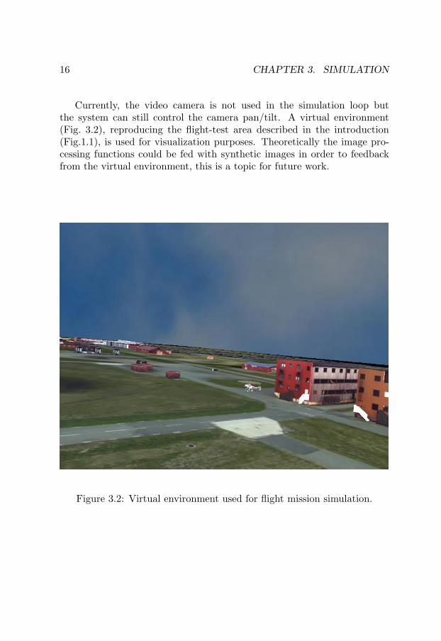
Currently, the video camera is not used in the simulation loop butthe system can still control the camera pan/tilt. A virtual environment(Fig. 3.2), reproducing the flight-test area described in the introduction(Fig.1.1), is used for visualization purposes. Theoretically the image pro-cessing functions could be fed with synthetic images in order to feedbackfrom the virtual environment, this is a topic for future work.
Figure 3.2: Virtual environment used for flight mission simulation.

3.3. REFERENCE FRAMES 17
3.3 Reference frames
This section provides an overview of the different reference frames used inthis thesis.
The Earth frame (Fig. 3.3) has its origin at the center of mass of theEarth and axes which are fixed with respect to the Earth. Its Xe axispoints toward the mean meridian of Greenwich, the Ze axis is parallel tothe mean spin axis of the Earth, and the Ye axis completes a right-handedorthogonal frame.
The navigation frame (Fig. 3.3) is a local geodetic frame which hasits origin coinciding with that of the sensor frame and axes with the Xn
axis pointing toward the geodetic north, the Zn axis orthogonal to the ref-erence ellipsoid pointing down, and the Yn axis completing a right-handedorthogonal frame.
Figure 3.3: Earth and navigation frames.
The body frame (Fig. 3.4) is an orthogonal axis set which has its origincoinciding with the center of gravity of the helicopter, the Xb axis pointingforward to the nose, the y-axis orthogonal to the Yb axis and pointing tothe right side of the helicopter body, and the Zb axis pointing down so that

18 CHAPTER 3. SIMULATION
it’s a right-handed orthogonal frame. Since the RMAX inertial sensors arequite close to the helicopter’s center of gravity it is possible to consider thenavigation frame and the body frame as having the same origin point.
Figure 3.4: Body frame.
In order to transform a vector from the body frame to the navigationframe a rotation matrix has to be applied:
Cnb =
cosθcosψ −cosφsinψ+sinφsinθcosψ sinφsinψ+cosφsinθcosψcosθsinψ cosφcosψ+sinφsinθsinψ −sinφcosψ+cosφsinθsinψ−sinθ sinφcosθ cosφcosθ
(3.1)
where φ, θ and ψ are the Euler angles roll, pitch and heading. Sincethe rotation matrix is orthogonal, the transformation from the navigationframe to the body frame is given by:
Cbn=(Cn
b )T (3.2)
The transformation matrix 3.1 and 3.2 will be used later in the thesis.

3.4. THE AUGMENTED RMAX DYNAMIC MODEL 19
3.4 The augmented RMAX dynamic model
The RMAX helicopter model presented in this thesis includes the bare he-licopter dynamics and the YACS control system dynamics. The code of theYACS is strictly Yamaha proprietary so the approach used to build the rel-ative mathematical model has been that of black-box model identification.With the use of this technique, it is possible to estimate the mathematicalmodel of an unknown system (the only hypothesis about the system is thatit has a linear behavior) just by observing its behavior. This is achieved inpractice by sending an input signal to the system and measuring its output.Once the input and output signals are known there are several methods toidentify the mathematical structure of the system.
The YACS model identification is not part of this thesis and detailscan be found in [4]. In the following section the transfer functions of theaugmented attitude dynamics will be given. These transfer functions willbe used to build the augmented RMAX helicopter dynamic model used inthe simulator.
3.4.1 Augmented helicopter attitude dynamics
As previously stated the YACS and helicopter attitude dynamics have beenidentified through black-box model identification.
The equations 3.3 represent the four input/output transfer functions inthe Laplace domain:
∆Φ =2.3(s2 + 3.87s+ 53.3)
(s2 + 6.29s+ 16.2)(s2 + 8.97s+ 168)∆AIL
∆Θ =0.5(s2 + 9.76s+ 75.5)
(s2 + 3s+ 5.55)(s2 + 2.06s+ 123.5)∆ELE (3.3)
∆R =9.7(s+ 12.25)
(s+ 4.17)(s2 + 3.5s+ 213.4)∆RUD
∆AZ =0.0828s(s+ 3.37)
(s+ 0.95)(s2 + 13.1s+ 214.1)∆THR
where ∆Φ and ∆Θ are the roll and pitch angle increments (deg), ∆R

20 CHAPTER 3. SIMULATION
the body yaw angular rate increment (deg/sec) and ∆AZ the accelerationincrement (g) along the Zb body axis. ∆AIL, ∆ELE, ∆RUD and ∆THRare the control input increments taken relative to a trimmed flight condi-tion. The control inputs are in YACS unit and range from -500 and +500.
These transfer functions describe not only the dynamic behavior of theYACS but also the dynamics of the helicopter (rotor and body) and thedynamics of the actuators.
Since the chain composed by the YACS, actuators and helicopter isquite complex it is important to remember that the estimated model hasonly picked up a simple reflection of the system behavior. The identificationwas done near the hovering condition so it is improper to use the modelfor different flight conditions. In spite of this, simulations up to ∼10 m/shave shown good agreement with the experimental flight-test results.
3.4.2 Helicopter equations of motion
The aircraft equations of motion can be expressed in the body referenceframe with three sets of first order differential equations [7]. The first setrepresents the translational dynamics along the three body axes:
X = m(u+ qw − rv) +mgsinθ
Y = m(v + ru− pw)−mgcosθsinφ (3.4)Z = m(w + pv − qu)−mgcosθcosφ
where X, Y , Z represent the resultants of all the aerodynamic forces; u,v, w the body velocity components; p, q, r the body angular rates; m andg the mass and the gravity acceleration; φ and θ the pitch and roll angles.
The second set of equations represents the aircraft rotational dynamics:
L = Ixp− (Iy − Iz)qrM = Iy q − (Iz − Ix)rp (3.5)N = Iz r − (Ix − Iy)pq
where L, M , N represent the moments generated by the aerodynamicforces acting on the helicopter; Ix, Iy, Iz the inertia moments of the heli-copter.

3.4. THE AUGMENTED RMAX DYNAMIC MODEL 21
The third set of equations represents the relation between the bodyangular rates and the Euler angles:
φ = p+ qsinφtanθ + rcosφtanθ
θ = qcosφ− rsinφ (3.6)ψ = qsinφsecθ + rcosφsecθ
These three sets of nonlinear equations are valid for a generic aircraft.The transfer functions in 3.3 can be used now in the motion equations.From the Laplace domain of the transfer functions, it is possible to passto the time domain. This means that from the first three equations in 3.3we derive φ(t), θ(t) and r(t) which can be used in 3.6 in order to find theother parameters p(t), q(t), ψ(t).
The equations in 3.5 will not be used in the model because the dynam-ics represented by these equations is contained in the first three transferfunctions in 3.3. The motion equations in 3.4 can be rewritten as follows:
u = Fx − qw + rv − gsinθ
v = Fy − ru+ pw + gcosθsinφ (3.7)w = Fz − pv + qu+ gcosθcosφ
where Fx, Fy, Fz are the forces per unit of mass. In this set of equationssome of the nonlinear terms are small and can be neglected for our flightenvelope, although for simulation purposes, it does not hurt to leave themthere. Later when the model will be used for control purposes the necessarysimplifications will be made.
The tail rotor force is included in Fy and it is balanced by a certainamount of roll angle. In fact every helicopter with a tail rotor must flywith a few degrees of roll angle in order to compensate for the tail rotorforce which is directed sideway. For the RMAX helicopter the roll angleis 4.5 deg in hovering condition with no wind. The yaw dynamics in ourcase is represented by the third transfer function in 3.3. For this reasonwe do not have to model the force explicitly. By doing that we find in ourmodel a zero degree roll angle in hovering condition which does not affect
22 CHAPTER 3. SIMULATION
substantially the dynamics of our simulator. Of course a small couplingeffect between the lateral helicopter motion and yaw channel is neglectedduring a fast yaw maneuver due to the consistent increase of the tail rotorforce.
The equations in 3.7 are than rewritten in find form as follows:
u = Xuu− qw + rv − gsinθ
v = Yvv − ru+ pw + gcosθsinφ (3.8)w = Zww + T − pv + qu+ gcosθcosφ
where Xu, Yv and Zw are the aerodynamic derivatives (accounting forthe aerodynamic drag). The value used for the aerodynamic derivatives areXu = −0.025, Yv = −0.1 and Zw = −0.6. These values have been chosenusing an empirical best fit criteria using flight-test data.
The main rotor thrust T is given by:
T = −g −∆aZ (3.9)
where ∆aZ is given by the fourth transfer function in 3.3.Comparing the equations in 3.8 with other works in the literature as for
example in [16] it can be noticed that the rotor flapping terms are missing(the rotor flapping represents the possibility of the helicopter rotor disk totilt relatively to the helicopter fuselage). On the other hand the flappingdynamics is contained in the transfer functions in 3.3. It was not possibleto model the rotor flapping explicitly in the equations 3.8 because it is notobservable from the black-box model identification approach used. Thefact that the flapping terms are not included in equations 3.8 does not havestrong consequences on the low frequency dynamics. On the other hand thehigh frequency helicopter dynamics is not captured correctly. Therefore thehelicopter model derived here cannot be used for high bandwidth controlsystem design. The model anyway is good enough for position and velocitycontrol loop design. In [20] the mathematical formulation for rotor flappingcan be found.
3.5. SIMULATION RESULTS 23
3.5 Simulation results
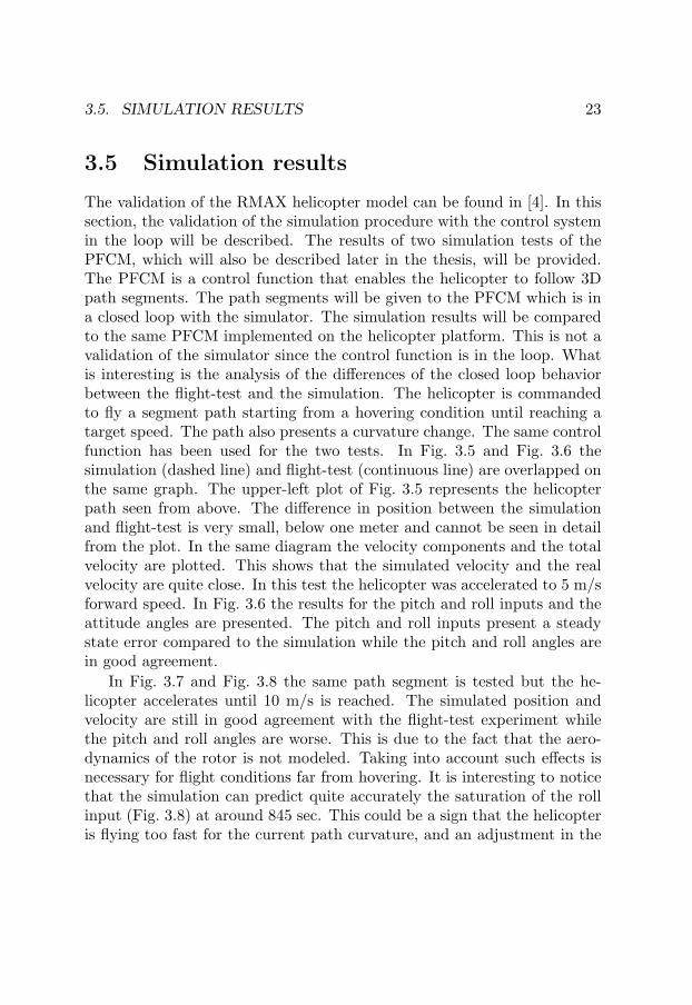
The validation of the RMAX helicopter model can be found in [4]. In thissection, the validation of the simulation procedure with the control systemin the loop will be described. The results of two simulation tests of thePFCM, which will also be described later in the thesis, will be provided.The PFCM is a control function that enables the helicopter to follow 3Dpath segments. The path segments will be given to the PFCM which is ina closed loop with the simulator. The simulation results will be comparedto the same PFCM implemented on the helicopter platform. This is not avalidation of the simulator since the control function is in the loop. Whatis interesting is the analysis of the differences of the closed loop behaviorbetween the flight-test and the simulation. The helicopter is commandedto fly a segment path starting from a hovering condition until reaching atarget speed. The path also presents a curvature change. The same controlfunction has been used for the two tests. In Fig. 3.5 and Fig. 3.6 thesimulation (dashed line) and flight-test (continuous line) are overlapped onthe same graph. The upper-left plot of Fig. 3.5 represents the helicopterpath seen from above. The difference in position between the simulationand flight-test is very small, below one meter and cannot be seen in detailfrom the plot. In the same diagram the velocity components and the totalvelocity are plotted. This shows that the simulated velocity and the realvelocity are quite close. In this test the helicopter was accelerated to 5 m/sforward speed. In Fig. 3.6 the results for the pitch and roll inputs and theattitude angles are presented. The pitch and roll inputs present a steadystate error compared to the simulation while the pitch and roll angles arein good agreement.
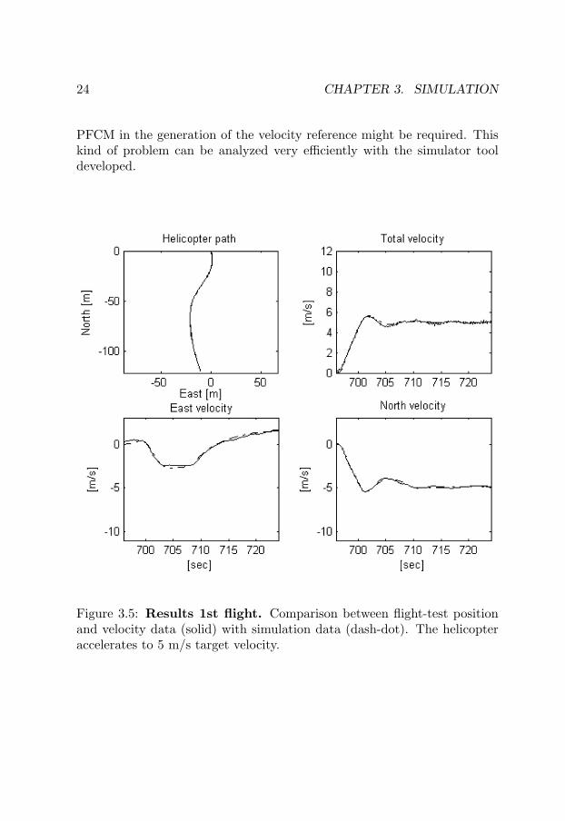
In Fig. 3.7 and Fig. 3.8 the same path segment is tested but the he-licopter accelerates until 10 m/s is reached. The simulated position andvelocity are still in good agreement with the flight-test experiment whilethe pitch and roll angles are worse. This is due to the fact that the aero-dynamics of the rotor is not modeled. Taking into account such effects isnecessary for flight conditions far from hovering. It is interesting to noticethat the simulation can predict quite accurately the saturation of the rollinput (Fig. 3.8) at around 845 sec. This could be a sign that the helicopteris flying too fast for the current path curvature, and an adjustment in the
24 CHAPTER 3. SIMULATION
PFCM in the generation of the velocity reference might be required. Thiskind of problem can be analyzed very efficiently with the simulator tooldeveloped.
Figure 3.5: Results 1st flight. Comparison between flight-test positionand velocity data (solid) with simulation data (dash-dot). The helicopteraccelerates to 5 m/s target velocity.

3.5. SIMULATION RESULTS 25
Figure 3.6: Results 1st flight. Comparison between flight-test helicopterinputs and attitude data (solid) with simulation data (dash-dot). Thehelicopter accelerates to 5 m/s target velocity.

26 CHAPTER 3. SIMULATION
Figure 3.7: Results 2nd flight. Comparison between flight-test positionand velocity data (solid) with simulation data (dash-dot). The helicopteraccelerates to 10 m/s target velocity.
3.5. SIMULATION RESULTS 27
Figure 3.8: Results 2nd flight. Comparison between flight-test helicopterinputs and attitude data (solid) with simulation data (dash-dot). Thehelicopter accelerates to 10 m/s target velocity.

28 CHAPTER 3. SIMULATION
3.6 Conclusion
In this chapter the simulation tool used to test and develop the UAV soft-ware architecture including the control system has been described. Thesimulator has been a useful tool for the development of the control modes.The hardware-in-the-loop version of the simulator is a useful tool to testa complete mission on the field. In addition, the fact that the helicopterservos are in the simulation loop provides a rapid verification that the rightsignals arrive from the control system. This verification is used for a finaldecision on the field in order to proceed or not with a flight-test.

29
Chapter 4
Path Following ControlMode
4.1 Introduction
The PFCM described in this chapter and presented in Paper I, has beendesigned to navigate an autonomous helicopter in an area cluttered withobstacles, such as an urban environment. In this thesis, the path plan-ning problem is not addressed although it is in [18]. It is assumed that apath planning functionality generates a collision-free path. Then the taskwhich will be solved here is to find a suitable guidance and control lawwhich enables the helicopter to follow the path robustly. The path plannercalculates the geometry of the path that the helicopter has to follow. Ageometric path segment, represented by a set of parameters, is then inputto the PFCM.
Before starting with the description of the PFCM, some basic terminol-ogy will be provided.
The guidance is the process of directing the movements of an aero-nautical vehicle with particular reference to the selection of a flight path.The term of guidance or trajectory generation in this thesis addresses theproblem of generating the desired reference position and velocity for the

30 CHAPTER 4. PATH FOLLOWING CONTROL MODE
helicopter at each control cycle.The outer control is a feedback loop which takes as inputs the reference
position and velocity generated by the trajectory generator and calculatesthe output for an inner control loop.
The inner control is a feedback loop which stabilizes the helicopterattitude and the vertical dynamics. As mentioned previously, the innercontrol loop used here has been developed by Yamaha Motor Companyand is part of the YACS.
Several methods have been proposed to solve the problem of generationand execution of a state-space trajectory for an autonomous helicopter [6,9]. In general this is a hard problem, especially when the trajectory is timedependent. The solution adopted here is to separate the problem into twoparts: first to find a collision-free path in the space domain [18] and thanto add a velocity profile later. In this way the position of the helicopter isnot time dependent which means that it is not required for the helicopterto be in a certain point at a specific time. A convenient approach for such aproblem is the path following method. By using the path following methodthe helicopter is forced to fly close to the geometric path with a specifiedforward speed. In other words, the path is always prioritized and this isa requirement for robots that for example have to follow roads and avoidcollisions with buildings. The method developed for PFCM is weakly modeldependent and computationally efficient.
The path following method has also been analyzed in [24, 22]. Theguidance law derived there presents singularity when the cross-track erroris equal to the curvature radius of the path so that it has a restriction on theallowable cross-track error. The singularity arises because the guidance lawis obtained by using the Serret-Frenet formulas for curves in the plane [24].
The approach used in this thesis does not use the Serret-Frenet formulasbut a different guidance algorithm similar to the one described in [5] whichis also known as virtual leader. In this case the motion of the control pointon the desired path is governed by a differential equation containing errorfeedback which gives great robustness to the guidance method. The controlpoint (Fig. 4.1) is basically a point lying on the path where the helicopterideally should be.
The guidance algorithm developed uses information from the modelin 3.8 described in section 3.4.2 in order to improve the path tracking

4.2. TRAJECTORY GENERATOR 31
Figure 4.1: Control point on the reference path.
error while maintaining a reasonable flight speed. The experimental resultspresented show the validity of the control approach.
Fig. 4.2 represents the different components of the control system, fromthe path planner to the inner loop that directly sends the control inputs tothe helicopter actuators. The PFCM described in this thesis includes thetrajectory generator and the outer control loop.
4.2 Trajectory generator
In this section, a description of the guidance algorithm developed for thePFCM is provided. The trajectory generator function takes as input a set ofparameters describing the geometric path calculated by the path plannerand calculates the reference position, velocity and heading for the innercontrol loop. First the analytic expression of the 3D path is calculated,then a feedback algorithm calculates the control point on the path. Finallythe reference input for the outer loop is calculated using the kinematichelicopter model described in chapter 3.

32 CHAPTER 4. PATH FOLLOWING CONTROL MODE
Figure 4.2: The PFCM includes two modules: trajectory generator andouter loop.
4.2.1 Calculation of the path geometry
The path planner generates 3D geometric paths described by a sequence ofsegments. Each segment is passed from the high-level part of the softwarearchitecture, where the path planner is located, to the low-level part wherethe control modes including the PFCM are implemented.
The path segment is generated in the navigation frame with the originfixed at the initial point of the path. We will use the superscript n toindicate a vector in the navigation frame. Each segment is described bya parameterized 3D cubic curve represented by the following equation invectorial form:
P n(s) = As3 +Bs2 +Cs+D (4.1)
where A,B,C and D are 3D vectors calculated from the boundaryconditions of the segment with s as the segment parameter.
4.2. TRAJECTORY GENERATOR 33
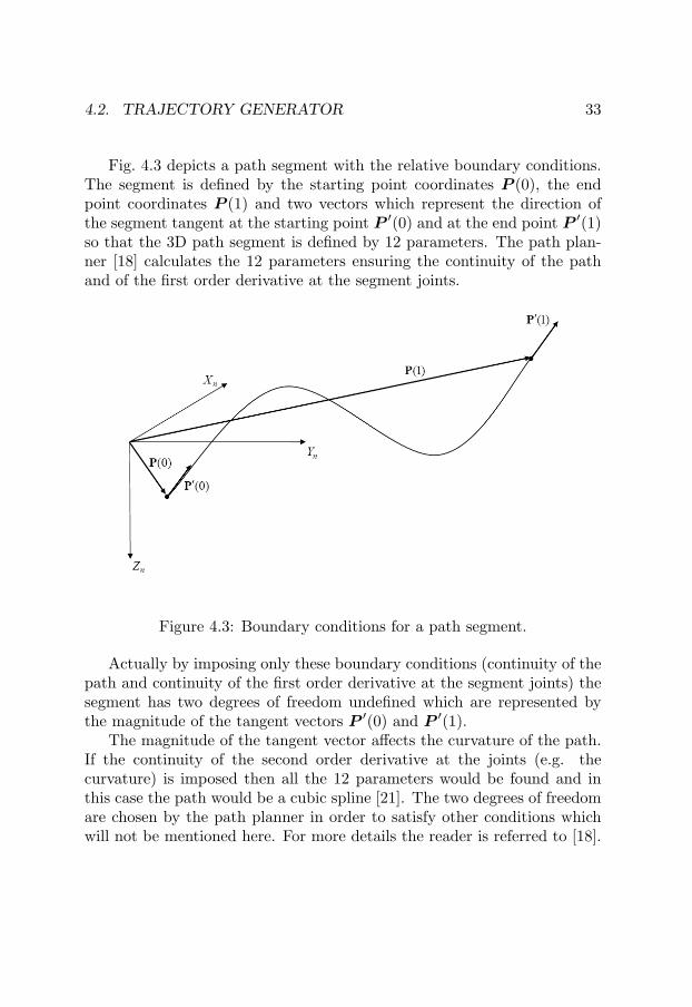
Fig. 4.3 depicts a path segment with the relative boundary conditions.The segment is defined by the starting point coordinates P (0), the endpoint coordinates P (1) and two vectors which represent the direction ofthe segment tangent at the starting point P ′(0) and at the end point P ′(1)so that the 3D path segment is defined by 12 parameters. The path plan-ner [18] calculates the 12 parameters ensuring the continuity of the pathand of the first order derivative at the segment joints.
Figure 4.3: Boundary conditions for a path segment.
Actually by imposing only these boundary conditions (continuity of thepath and continuity of the first order derivative at the segment joints) thesegment has two degrees of freedom undefined which are represented bythe magnitude of the tangent vectors P ′(0) and P ′(1).
The magnitude of the tangent vector affects the curvature of the path.If the continuity of the second order derivative at the joints (e.g. thecurvature) is imposed then all the 12 parameters would be found and inthis case the path would be a cubic spline [21]. The two degrees of freedomare chosen by the path planner in order to satisfy other conditions whichwill not be mentioned here. For more details the reader is referred to [18].

34 CHAPTER 4. PATH FOLLOWING CONTROL MODE
The path generated in this way can have discontinuity of the second orderderivative at the segment joints. This can lead to a small path trackingerror especially at high speed.
The 12 parameters are passed as input arguments to the PFCM whichthen generates the reference geometric segment used for control purposes.The generation of the path segment in the PFCM is done using the matrixformulation in 4.2 with the boundary condition vector explicitly written onthe right hand side. The parameter s ranges from s = 0 which correspondsto the starting point P (0) to s = 1 which corresponds to the end pointP (1) of the same segment. When the helicopter enters the next segmentthe parameter is reset to zero.
P n(s) =[s3 s2 s 1
] 2 −2 1 1−3 3 −2−10 0 1 01 0 0 0
P (0)P (1)P ′(0)P ′(1)
(4.2)
For control purposes the tangent and the curvature need to be calcu-lated. The path tangent T n is:
T n(s) =[
3s2 2s 1 0]
2 −2 1 1−3 3 −2−10 0 1 01 0 0 0
P (0)P (1)P ′(0)P ′(1)
(4.3)
The path curvature Kn is:
Qn(s) =[
6s 2 0 0]
2 −2 1 1−3 3 −2−10 0 1 01 0 0 0
P (0)P (1)P ′(0)P ′(1)
Kn(s)=
T n(s)×Qn(s)× T n(s)|T n(s)|4
(4.4)
In the guidance law the curvature radius which is Rn = 1/Kn will beused. Since T n and Rn are expressed in the navigation frame, in order to

4.2. TRAJECTORY GENERATOR 35
be used in the guidance law, they have to be transformed into the bodyframe using the rotation matrix Cb
n defined in section 3.3.At this point the geometric parameters (tangent and curvature) of the
path segment are known. Now these parameters can be used in the guidancelaw provided that the path segment parameter s is known. The method asto how to find s will be discussed in the next section.
4.2.2 Feedback method
When the dynamic model of the helicopter is known, it is in principlepossible to calculate beforehand at what point in the path the helicoptershould be at a certain time. By doing this the path segment would be timedependent. In this way at each control cycle the path parameters (position,velocity and attitude) would be known and they could be used directly forcontrol purposes. Then the helicopter could be accelerated or slowed downif it is behind or ahead of the actual control point (which is the point ofthe path where the helicopter should be at the relative time).
The generation of a time dependent trajectory is usually a complexproblem. An additional complication is that the trajectory has to satisfyobstacle constraints (to find a collision free path in a cluttered environ-ment [18]).
The alternative approach used here is the following. Instead of acceler-ating or slowing down the helicopter, the control point will be acceleratedor slowed down using a feedback method. In this way the path is not timedependent anymore and so the problem of generating a collision free pathcan be treated separately from the helicopter dynamics. Of course the pathgenerated must be smooth enough to be flown with a reasonable velocityand this has to be taken into account at the path planning level. The factthat the helicopter kinematic and dynamic constraints are not taken intoaccount at the path planning level might lead to a path which forces thehelicopter to abrupt brake due to fast curvature change. This problem canbe attenuated using some simple rules in the calculation of the segmentboundary conditions [18].
The algorithm implemented in this thesis finds the control point bysearching for the closest point of the path to the helicopter position. Theproblem could be solved geometrically simply by computing an orthogonal

36 CHAPTER 4. PATH FOLLOWING CONTROL MODE
projection from the helicopter position to the path. The problem whicharises in doing this is that there could be multiple solutions. For this reasona method has been adopted which finds the control point incrementally andsearches for the orthogonality condition only locally.
The reference point on the nominal path is found by satisfying thegeometric condition that the scalar product between the tangent vectorand the error vector has to be zero:
E • T = 0 (4.5)
where the error vector E is the helicopter distance from the candidatecontrol point. The control point error feedback is calculated as follows:
ef = E • T /|T | (4.6)
that is the magnitude of the error vector projected on the tangent T .The vector E is calculated as follows:
E = pcp,n−1 − pheli (4.7)
where pcp,n−1 is the control point position at the previous control cycleand pheli is the actual helicopter position. The control point is updatedusing the differential relation:
dp = p′ · ds (4.8)
Equation 4.8 is applied in the discretized form:
sn = sn−1 +ef
|dpcp
ds |n−1
(4.9)
where sn is the new value of the parameter. Equations 4.6 and 4.9can also be used iteratively in order to find a more accurate control pointposition. In this application, it was not necessary. Once the new value ofs is known, all the path parameters can be calculated.

4.2. TRAJECTORY GENERATOR 37
4.2.3 Outer loop reference inputs
In this section, the method used to calculate the reference input or set-pointfor the outer control loop will be described in detail. Before proceeding, adescription as to how the PFCM takes into account some of the helicopterkinematic constraints will be provided.
PFCM kinematic constraints
The model in 3.8 will be used to derive the guidance law which enables thehelicopter to follow a 3D path.
The sin and cos can be linearized around θ = 0 and φ = 0 since in ourflight condition, the pitch and roll angles are between the interval ∼ ±20deg. This means that we can approximate the sin of the angle to the angleitself (in radians) and the cos of the angle to 1. By doing this from thefirst and second equation of 3.6 it is possible to calculate the body angularrate p and q:
q = θ + rφ (4.10)p = φ− rθ
where the product between two or more angles has been neglected be-cause it is small compared to the other terms. Using the same considera-tions and substituting 4.10 it is possible to rewrite the system in 3.8 in thefollowing form:
u = Xuu− (θ + rφ)w + rv − gθ
v = Yvv − ru+ (φ− rθ)w + gφ (4.11)w = Zww + T − (φ− rθ)v + (θ + rφ)u+ g
At this point we can add the condition that the helicopter has to fly withthe fuselage aligned to the path (in general this condition is not necessaryfor a helicopter, it has been adopted here to simplify the calculation). Theconstraints which describe this flight condition (under the assumption ofrelatively small pitch and roll angles) are:

38 CHAPTER 4. PATH FOLLOWING CONTROL MODE
r =u
Rby
θ =u
Rbz
(4.12)
v = v = 0w = w = 0
where Rby and Rb
z are the components of the curvature radius along thebody axes Yb and Zb, respectively.
The equations in 4.11 can finally be rewritten as:
r =u
Rby
θ =Xuu− u
g
φ =u2
gRby
(4.13)
T = − u2
Rbz
− u4
g(Rby)2
− g
In the right hand side of 4.13 we have the four inputs that can be givenas a reference signal to an inner control loop (like the YACS) which controlsthe yaw rate r, the attitude angles φ, θ and the rotor thrust T . These inputsonly depend on the desired velocity and acceleration u and u and the pathcurvature Rb
y and Rbz.
If the geometry of the path, which is represented by Rby and Rb
z, isthen assigned, in principle it is possible to assign a desired velocity andacceleration u and u and calculate the four inputs for the inner loop. Theproblem is that these inputs cannot be assigned arbitrarily because theyhave to satisfy the constraints of the dynamic system composed by thehelicopter plus the inner loop.
A solution of 4.13 which does not involve the dynamic constraints isrepresented by a stationary turn on the horizontal plane with constant
4.2. TRAJECTORY GENERATOR 39
radius (picture (a) of Fig. 4.4). The solution for this flight condition is givenby 4.13 where Rb
z = ∞, u = 0 and Rby = constant. This condition is called
trimmed flight because the first derivative of the flight parameters are zero(φ = θ = r = T = u = 0). For this flight condition it is straightforward tocalculate the maximum flight speed allowed. Since the maximum values ofr, φ, θ and T are limited for safety reasons, the maximum path velocity ucan be calculated from the system 4.13:
u1 = |Rbyrmax|
u2 = |gθmax
Xu|
u3 =√|φmaxgRb
y| (4.14)
u4 = (| − g(Tmax + g)(Rby)2|) 1
4
The minimum of these four velocities can be taken as the maximumspeed for the path:
umax = min(u1, u2, u3, u4) (4.15)
The path generated by the path planner is represented by a cubic poly-nomial. The curvature radius in general is not constant for such a path,which means that the helicopter never flies in trimmed conditions but itflies instead in maneuvered flight conditions.
Let’s now examine a maneuver in the vertical plane (Rby = ∞, Rb
z =constant). From the second equation in 4.12 and the second equationin 4.13 we can observe that there is no constant velocity solution (u = 0)which satisfies both. This means that when the helicopter climbs, it losesvelocity.
To make the PFCM more flexible in the sense of allowing vertical climb-ing and descending at a constant speed, we have to remove the constraintθ = u/Rb
z and w = w = 0. In other words the fuselage will not be alignedto the path during a maneuver in the vertical plane as it is shown in Fig. 4.4(c). The helicopter instead will follow the path as it is shown in Fig. 4.4(b).

40 CHAPTER 4. PATH FOLLOWING CONTROL MODE
a) XY path b) XZ path
V
c) XZ path with fuselage aligned
bX
bZ
bY
bX
XYR XZR
bZ
V
XZR
V
bX
Figure 4.4: Representation of the several ways in which the helicopter canfollow a 3D path.
4.2. TRAJECTORY GENERATOR 41
Calculation of the outer loop inputs
We can finally address the problem of generating the reference inputs forthe outer control loop. The inputs will be calculated in the form of controlerrors (difference between the current helicopter state and the desired one)as follows.
1. Calculation of the position error vector δp.
The position error vector is the difference between the control pointposition pn
cp and the helicopter position given by the INS/GPS systempn
heli. In order to be used in the outer loop control equations thevector must be rotated from the navigation frame to the body frameusing the rotation matrix Cb
n:
δpb = Cbn(pn
cp − pnheli)
As explained in section 4.2.2, the control point position is calculatedusing feedback from the helicopter position. The method does notsearch for the control point along the whole path segment but itremembers the value of the parameter s (e.g. the previous controlpoint) from the previous control cycle and starts the search fromthere. By doing this, the search is very fast since the new controlpoint will not be far from the previous one (the control function iscalled with a frequency of 50Hz). At the beginning of each segment,the parameter value is set to zero.
Once the new value of s is found, the position error vector δpb canbe calculated together with the local path tangent T and curvatureK.
2. Calculation of the velocity error vector δv.
The velocity error vector is the difference between the target velocityvtarg and the helicopter velocity given by the INS/GPS system vn
heli.The target velocity is obviously tangent to the geometric path. Thedirection of the tangent vector is given by:

42 CHAPTER 4. PATH FOLLOWING CONTROL MODE
τn =T n
|T |(4.16)
In order to be used in the control equations in 4.24, the velocity errorvector must be expressed in the body frame in the same way as theposition error vector:
δvb = Cbn(vtarg · τn − vn
heli) (4.17)
The calculation of vtarg (desired helicopter velocity along the path)must take into account the helicopter kinematic constraints, the lim-itation due to the maximum allowable vertical velocity and the par-ticular phase of the flight path that is acceleration, cruising andbraking.
Let us call vtarg1 the velocity calculated according to the acceleration,cruising and braking condition, vtarg2 the velocity calculated accord-ing to the helicopter kinematic constraints and vtarg3 the velocityaccording to the vertical speed limitation. These three velocities willbe calculated in the following part of this section and the minimumvalue among the three will be used as vtarg. This procedure is re-peated at each control cycle and in this way the velocity profile forthe path is shaped.
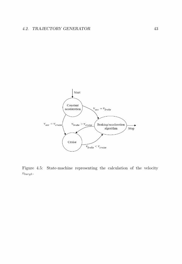
The calculation of vtarg1 is done considering the acceleration, cruisingand braking conditions. The calculation scheme can be representedby the state-machine in Fig. 4.5.
The constant acceleration phase is activated only at the beginningof the first segment of the path and it ends when vacc=vcruise orvacc=vbrake. vcruise is set by the path planner while the calculationof vbrake will be explained below. During the acceleration phase vacc
is increased at a constant rate of 1.2 m/s2. The cruising phase isactive when the braking and the acceleration phases are off. The
4.2. TRAJECTORY GENERATOR 43
Figure 4.5: State-machine representing the calculation of the velocityvtarg1.
44 CHAPTER 4. PATH FOLLOWING CONTROL MODE
braking condition is activated when the following condition becomestrue:
vbrake < vcruise (4.18)
with
vbrake =√|(2 · lend ·Acc+ v2
end)| (4.19)
where lend is the distance, calculated along the path segment, thatthe helicopter has to fly to reach the end of the segment and Acc isthe desired acceleration during the braking phase (its value is set to1.2 m/s). vend is the desired velocity at the end of each path segmentand it is assigned by the path planner. The condition 4.18 means thatthe helicopter must start to brake when the distance to the end ofthe segment is equal to the distance necessary to bring the helicopterfrom the velocity vcruise to vend with the desired acceleration. If vend
is greater than vcruise the helicopter increases the velocity instead.The method used for the calculation of lend is explained in Paper I.
The calculation of vtarg2 takes into account the kinematic constraintsdescribed by the equations in 4.14. For safety reasons the flight enve-lope has been limited to: rmax = 40 rad/sec maximum yaw rate, φmax
= 15 deg maximum roll angle, θmax = 15 deg maximum pitch angleand for the vertical acceleration a load factor of Nzmax = Tmax/g =1.1. The value of Nzmax has been chosen using the fact that Nzmax
= 1.1 means increasing the helicopter weight 10 percent. The max-imum takeoff weight of the RMAX is 94kg and the RMAX weightused in this experimental test is around 80kg, so a load factor of 1.1ensures enough safety. The second equation in 4.14 represents theforward velocity u2 achievable with the maximum pitch angle. It isnot considered as a constraint here since the cruise velocity assigned
4.2. TRAJECTORY GENERATOR 45
by the path planner will always be smaller than u2. umax is calculatedusing 4.15. Finally we can calculate vtarg2 as:
vtarg2 =umax
τ bx
(4.20)
where τ bx is the projection of the vector in 4.16 on the helicopter Xb
body axis.
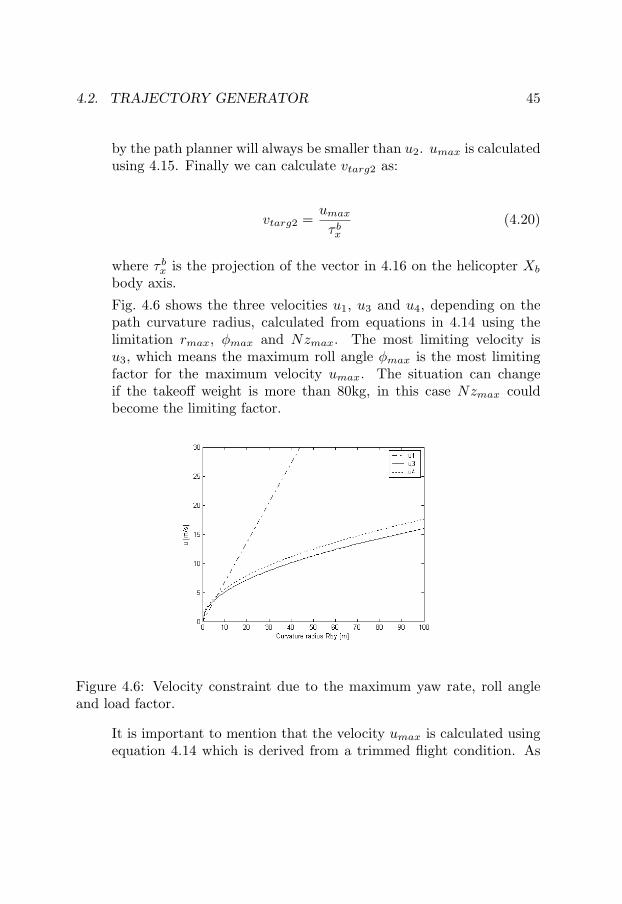
Fig. 4.6 shows the three velocities u1, u3 and u4, depending on thepath curvature radius, calculated from equations in 4.14 using thelimitation rmax, φmax and Nzmax. The most limiting velocity isu3, which means the maximum roll angle φmax is the most limitingfactor for the maximum velocity umax. The situation can changeif the takeoff weight is more than 80kg, in this case Nzmax couldbecome the limiting factor.
Figure 4.6: Velocity constraint due to the maximum yaw rate, roll angleand load factor.
It is important to mention that the velocity umax is calculated usingequation 4.14 which is derived from a trimmed flight condition. As

46 CHAPTER 4. PATH FOLLOWING CONTROL MODE
previously mentioned, using a path described by a cubic polynomial,the curvature changes continuously and the helicopter almost neverflies in trimmed conditions. The resulting umax might not always beconsistent with the attitude dynamics θ and φ. The faster the speed,the more the attitude dynamics is relevant.
The velocity vtarg3 is calculated as follows. The vertical velocitymust be limited during a descending path because of the vortex ringwhich can build up around the main rotor in this flight condition.In this case, the helicopter descends into rotor down-wash and enterswhat is commonly called the vortex ring state (VRS). This situationcan cause loss of helicopter control and might be difficult to recover.For this reason a limitation on the descending velocity component isnecessary. The flow state diagram of Fig. 4.7 shows the combinationof horizontal and vertical speed where VRS occurs. This diagram wasdeveloped at the Aviation Safety School, Monterey CA, in the late1980s for use by mishap investigators in their analysis of several ofthese events. In this thesis, this diagram has been used as a guidelinein choosing the right combination of vertical and horizontal speed inorder to avoid a VRS situation. More details on VRS phenomenoncan be found in [20].
The flow state diagram axes are parametrized with the hovering in-duced velocity which is calculated in feet/minutes as follows:
Vi = 60
√DL
2ρ(4.21)
where DL is the rotor disk loading (lbs/ft2) and ρ the air density(SLUGS
ft3 ). This diagram will be used to calculate a safe vertical speed.
For the RMAX helicopter, the induced hovering velocity calculatedusing 4.21 and converted in m/s results in Vi=6.37 m/s. The value hasbeen calculated using the air density at sea level ρ = 0.002377SLUGS
ft3 ,RMAX weight of 80 kg and rotor diameter R=3.115 m. From thediagram, the vertical speed when the light turbulence first occurs is

4.2. TRAJECTORY GENERATOR 47
Figure 4.7: Flow states in descending forward flight.

48 CHAPTER 4. PATH FOLLOWING CONTROL MODE
around w1=0.5Vi=3.18 m/s. It can also be observed that for a descentangle smaller than 30 deg the VRS area is avoided completely.
The maximum vertical velocity profile chosen for the RMAX is shownin Fig. 4.8 (dashed line) where for safety reasons w1 has been reducedto 1.5 m/s for a descent angle γ greater than 30 deg, while for γsmaller then 30 deg the descending velocity has been limited to w2 =3 m/s.
Figure 4.8: Maximum descent velocity used in the PFCM for the RMAXhelicopter.
The calculation of vtarg3 is then:
γ = atan(τnz
τnx
)
wMAXdescent = 1.5 90 > γ ≥ 30
wMAXdescent = 3 30 > γ > 0 (4.22)
vtarg3 =wMAXdescent
τnz
4.3. OUTER LOOP CONTROL EQUATIONS 49
Finally, the helicopter velocity profile is given by:
vtarg = min(vtarg1, vtarg2, vtarg3)
3. Calculation of the heading error δψ.
The heading error is given by:
δψ = atan2(Tny , T
nx )− ψheli
where ψheli is the helicopter heading given by the INS/GPS system.
4. Calculation of the feed forward control terms rff , φff .
The terms rff and φff are calculated from the first and third equa-tions in 4.13 where the component of the curvature radius Rb
y is cal-culated as follows:
Kb = CnbK
n
Rby =
1Kb
y
(4.23)
The feed forward terms will be used in the outer control loop toenhance the tracking precision.
4.3 Outer loop control equations
The PFCM control equations implemented on the RMAX are the following:

50 CHAPTER 4. PATH FOLLOWING CONTROL MODE
Y AWyacs = rff +Ky1 δψ
PITCHyacs = Kp1 δpx +Kp
2 δvx +Kp3
d
dtδvx +Kp
4
∫δvxdt
ROLLyacs = φff +Kr1δpy +Kr
2δvy (4.24)
THRyacs = Kt1δpz +Kt
2δvz +Kt3
∫δvzdt
where the K’s are the control gains, rff and φff are the feed-forward controlterms resulting from the model in 4.13. The other two terms θff and Tff
relative to the pitch and throttle channels have not been implemented.These channels are controlled by the feedback loop only. δψ is the headingerror, δp is the position error vector (difference between the control pointand helicopter position), δv is the velocity error vector (difference betweentarget velocity and helicopter velocity).
Adding the feed forward control terms, especially on the roll channel,results in a great improvement in the tracking capability of the control sys-tem compared to a PID feedback loop only. Results of the control approachare shown in the next section.
4.4 Experimental results
This section presents experimental results of the PFCM implemented on theRMAX helicopter. In Fig. 4.9, a 3D path is flown starting from an altitudeof 40 meters and finishing at 10 meters. The path describes a descendingspiral and the velocity vcruise given by the path planner was set to 10 m/s.In Fig. 4.10, the velocity profile of the path is represented and it can beobserved that as soon as the helicopter reaches 10 m/s it slows down inorder to make the turn with the compatible velocity. This was an earlytest, where the roll angle limitation was quite strict (around 8 deg). Thisexplains the consistent decreasing velocity. In addition, the accelerationphase was missing. In fact, the commanded target velocity, represented bythe dashed line, starts at 10 m/s. This resulted in an abrupt pitch input atthe beginning of the flight. Results of several trials of the same path flownwith different wind conditions are shown in Paper I.

4.4. EXPERIMENTAL RESULTS 51
−100
1020
3040
50
−100
−90
−80
−70−60
−50
−40
−30
−20
−100
0
10
20
30
40
50
60
East [m]
North [m]
Up
[m]
Flight TestTarget
A
B
Figure 4.9: Target and actual 3D helicopter path.
490 495 500 505 510 515 520 5250
2
4
6
8
10
12
Time [sec]
Spe
ed [m
/s]
flight testtarget
Figure 4.10: Target and actual helicopter speed.

52 CHAPTER 4. PATH FOLLOWING CONTROL MODE
Although the PFCM just described has exhibited a satisfactory perfor-mance in terms of robustness, the tracking capabilities in case of maneu-vered flight (when path curvature change rapidly) were not satisfactory.For this reason, the possibility to improve the tracking performance wasinvestigated in the case of maneuvered flight without a major redesign ofthe control system.
The lateral control has been modified by adding an extra control loop onthe roll channel besides the YACS control system. The new lateral controlloop is depicted in Fig. 4.11 b). From the diagram one can compare thedifference between the previous control scheme, Fig. 4.11 a), and the newone Fig. 4.11 b).
Figure 4.11: a)Previous lateral control. b)Modified lateral control loopusing a lead compensator.
The inner compensator that was added provides a phase lead compen-sation with an integral action and has the following structure:
4.5. CONCLUSIONS 53
C(s) = K(α1 + s
1 + αs) +KI
1s
(4.25)
The phase lead compensation increases the bandwidth and, hence, makesthe closed loop system faster, but it also increases the resonance frequencywith the danger of undesired amplification of system noise. The controlsystem has been tuned in simulation but a second tuning iteration wasneeded on the field due to the presence of damped oscillations on the rollchannel.
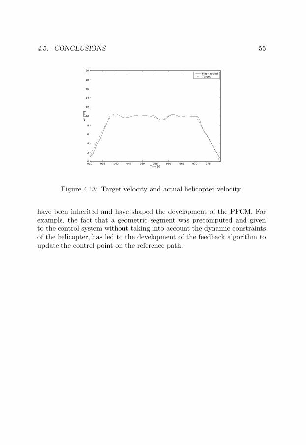
An experimental comparison between the modified control system andthe previous one is shown in Fig. 4.12. The target velocity in both caseswas set to 10 m/s. Fig. 4.13 depicts the target velocity and the actualhelicopter velocity relative to the path on the right side of Fig. 4.12. Thediagram on the right side in Fig. 4.12 depicts the path flown with the basicPFCM controller (Fig. 4.11 a). One can observe that in the dynamic partof the path, where the curvature changes rapidly, the controller is slow.This results in a relevant tracking error.
The diagram on the left in Fig. 4.12 depicts a test of the same pathflown with the modified roll control loop (Fig. 4.11 b). The new lateralcontrol scheme improves the tracking capability in the presence of fastcurvature change. The helicopter can follow the dynamic part of the pathwith considerably lower tracking error.
4.5 Conclusions
The PFCM developed here has been integrated in the helicopter softwarearchitecture and it is currently used in a number of flight missions carriedout in an urban area used for flight-tests. The goal has been the devel-opment of a reliable and flexible flight mode which could be integratedrobustly with a path planner. Safety mechanisms have been built-in thePFCM in order to handle communication failures with the path planner(this can happen since the path planner is implemented on a separate com-puter). More details on this topic can be found in Paper I. Moreover, sincethe path planner was developed before the PFCM, a number of constraints

54 CHAPTER 4. PATH FOLLOWING CONTROL MODE
Figure 4.12: Comparison of path tracking performances using two differentroll control strategy. On the right side is depicted the flight-test of themodified roll control loop with the lead compensator added. On the leftthe same test is done using the old roll control configuration. The flight-tests were performed at 36 km/h velocity for both paths.
4.5. CONCLUSIONS 55
930 935 940 945 950 955 960 965 970 9750
2
4
6
8
10
12
14
16
18
20
Time [s]
Vel
[m/s
]
Flight testedTarget
Figure 4.13: Target velocity and actual helicopter velocity.
have been inherited and have shaped the development of the PFCM. Forexample, the fact that a geometric segment was precomputed and givento the control system without taking into account the dynamic constraintsof the helicopter, has led to the development of the feedback algorithm toupdate the control point on the reference path.

56 CHAPTER 4. PATH FOLLOWING CONTROL MODE

57
Chapter 5
Sensor fusion for visionbased landing
This chapter describes the sensor fusion approach applied to a vision basedlanding capability described in Paper III.
The vision based autonomous landing mode developed during the WITASProject has been tested on the RMAX helicopter. It allows the helicopterto successfully complete a landing maneuver autonomously from an alti-tude of about 20 meters using only a single camera and inertial sensors(GPS is not used). An artificial landing pattern has been designed and itis placed on the ground during the landing maneuver. An on-board videocamera, mounted on a pan-tilt mechanism, locks on the pattern while animage processing algorithm computes the relative position of the on-boardcamera and the pattern. This position is then used in the sensor fusionfilter described in this chapter in order to provide reliable helicopter statefor the autonomous landing. During the landing phase a pan-tilt controllertracks the pattern keeping it in the middle of the image. This feature in-creases the robustness of the landing approach described here, minimizingthe possibility of loosing the pattern from the camera view due to acciden-tal, abrupt helicopter movements.
Vision based autonomous landing is a complex problem and it requires

58 CHAPTER 5. SENSOR FUSION FOR VISION BASED LANDING
competences in several disciplines such as image processing, sensor fusionand control. Paper III describes the approach and solution to the completeproblem. This chapter focuses on the sensor fusion problem involved in thevision based autonomous landing mode. Details of the image processingand control strategy are not described here. The reader interested in thedetails of these problems should read Paper III in the appendix of thisthesis.
The motivations for the development of a vision based landing mode areof two categories: scientific and technical. The scientific motivation is that ahelicopter which does not rely on external sources of information (like GPS)contributes to the scientific goal of a self-sufficient autonomous system.The technical motivation is that GPS technology is generally not robustwhile operating close to obstacles. For example, in an urban environmentthe GPS signal can be obscured by buildings or corrupted by multi pathreflections or nearby radio frequency transmitters. The landing approachproposed in Paper III is completely independent of a GPS, so it can beused for landing the helicopter in proximity of obstacles found in urbanenvironments.
In order to stabilize and control a UAV helicopter, an accurate andreliable state estimation is required. The standard strategy to solve thisproblem is to use several sensors with different characteristics, such asinertial sensors and GPS, and fuse them together using a Kalman filter.The integration between inertial sensors and GPS is a common practiceand an extensive literature on this topic is available. Several approaches tothis problem can be found in [13, 25, 23].
The method used here to fuse vision data with inertial sensors is similarto that used for GPS and inertial sensor integration with a number ofdifferences in the implementation. The great experience gained in manysuccessful experimental landings with our RMAX platform provides strongconfirmation that the same sensor integration technique used for GPS andinertial sensors can be used when the GPS is replaced with a suitable imageprocessing system. The vision based landing problem for an unmannedhelicopter has been addressed by other research groups, some related workon this problem can be found in Paper III.
As already mentioned, the landing problem is solved by using a singlecamera mounted on a pan-tilt unit and an inertial measurement unit (IMU)
59
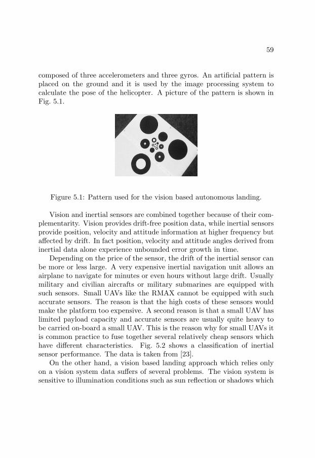
composed of three accelerometers and three gyros. An artificial pattern isplaced on the ground and it is used by the image processing system tocalculate the pose of the helicopter. A picture of the pattern is shown inFig. 5.1.
Figure 5.1: Pattern used for the vision based autonomous landing.
Vision and inertial sensors are combined together because of their com-plementarity. Vision provides drift-free position data, while inertial sensorsprovide position, velocity and attitude information at higher frequency butaffected by drift. In fact position, velocity and attitude angles derived frominertial data alone experience unbounded error growth in time.
Depending on the price of the sensor, the drift of the inertial sensor canbe more or less large. A very expensive inertial navigation unit allows anairplane to navigate for minutes or even hours without large drift. Usuallymilitary and civilian aircrafts or military submarines are equipped withsuch sensors. Small UAVs like the RMAX cannot be equipped with suchaccurate sensors. The reason is that the high costs of these sensors wouldmake the platform too expensive. A second reason is that a small UAV haslimited payload capacity and accurate sensors are usually quite heavy tobe carried on-board a small UAV. This is the reason why for small UAVs itis common practice to fuse together several relatively cheap sensors whichhave different characteristics. Fig. 5.2 shows a classification of inertialsensor performance. The data is taken from [23].
On the other hand, a vision based landing approach which relies onlyon a vision system data suffers of several problems. The vision system issensitive to illumination conditions such as sun reflection or shadows which

60 CHAPTER 5. SENSOR FUSION FOR VISION BASED LANDING
Figure 5.2: Inertial sensor performance classification. The data are takenfrom [23].
can partially cover the pattern. In these situations the vision system isblind and does not deliver any position data. A clever landing controlis to choose the best approach in order to avoid these situations usingthe knowledge of the sun position as explained in Paper III, but this isnot always compatible with the wind direction which is also a factor whendetermining the landing approach. Also the pattern view can be lost beforetouching down when the helicopter is very close to the pattern. In fact, itis hard for the camera pan-tilt control to track the pattern in this situation.Therefore in case the vision system does not deliver position informationfor a short time, the dead-reckoning capability of the filter can still deliveruseful information to continue the landing maneuver. This capability willbe shown in the experimental results.
By fusing inertial and vision data together using the Kalman filter tech-nique, it is possible to obtain a reliable high frequency and drift-free heli-copter state estimation. Sensor integration also allows low latency velocityestimation which is essential for stable helicopter control. Nevertheless the

5.1. FILTER ARCHITECTURE 61
filter provides more accurate attitude angles information than the one givenby vision only as will be shown by the experimental results.
5.1 Filter architecture
The filter developed is composed of two main functions: the INS mecha-nization function and the Kalman filter function. The INS mechanizationfunction performs the time integration of the inertial sensors while theKalman filter function estimates the errors of the INS mechanization. Theerrors estimated by the Kalman filter are then used to correct the finalsolution and are fed back into the mechanization process. The feedbackarchitecture is shown in Paper III.
5.1.1 Filter initialization
The filter turns on automatically as soon as the first valid data from thevision system is available, then the first step is the calculation of the headingof the helicopter relative to the pattern. The heading is given directly bythe vision system but a median filter over two seconds period is appliedon the raw vision heading. The results from the median filter are taken asinitial heading for the filter initialization. The assumption is that duringthe two seconds after the filter has turned on, the helicopter does not makeany large yaw maneuver. Otherwise the median value might differ toomuch from the initial heading. The raw vision heading is not used directlyin order to avoid the risk of initializing the filter with an outlier. Theinitialization of the heading is done carefully because the convergence ofthe filter to the correct heading is very slow when the helicopter is near ahovering condition, which is true in the case of a landing maneuver.
Once the heading is available, the filter can be initialized. The rawrelative position coming from the vision system is taken as initial position.The vertical and horizontal velocities are initialized to zero since the landingapproach starts from a hovering condition. Even if the initial position andvelocity have a relatively small error, the filter converges very fast to theright value since the covariance of the vision measurement is quite low. Theinitial pitch and roll angles are taken directly from the Yamaha Attitude

62 CHAPTER 5. SENSOR FUSION FOR VISION BASED LANDING
Sensor (YAS). The YAS sensor has been introduced in section 2.2. Theseangles are only used to initialize the filter and are not used again duringthe landing. In this way the filter initialization does not rely on GPS at alland so the vision based positioning system is completely independent fromit.
After the filter has been initialized the system waits ten seconds tomake sure that all the filter parameters have converged before the land-ing procedure can begin. If the vision capability is lost during this time,the initialization procedure starts again from scratch. During the land-ing procedure, consistency checks are made in order to detect and rejectmeasurement outliers from the vision system. In Paper III, details of themonitoring scheme implemented are given.
5.1.2 INS mechanization
The INS mechanization function implements and solves the navigation dif-ferential equations given in 5.1.
rn = vn
vn = Cnbf
b−(2ωnie+ω
nen)×vn+gn (5.1)
Cn
b = Cnb (Ωb
ib −Ωbin)
where rn is the position , vn the velocity and Cnb the direction cosine
matrix of the attitude angles calculated relative to a local navigation frame.In addition f b and Ωb
ib are the accelerometer and gyro outputs, gn is thegravity vector and ωn
ie the Earth rotation rate.The calculation of the attitude angles is made using a quaternion rep-
resentation because the linearity of the differential equations allows foran efficient implementation [8]. Details of the implementation of the INSmechanization can be found in [23].
5.1.3 Kalman filter
The Kalman filter implementation utilizes a 12-state linear INS error modelof which nine navigation error states (latitude, longitude and altitude error;
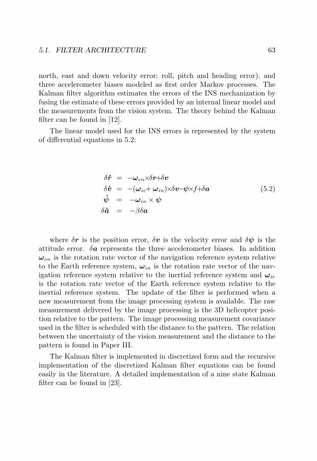
5.1. FILTER ARCHITECTURE 63
north, east and down velocity error; roll, pitch and heading error), andthree accelerometer biases modeled as first order Markov processes. TheKalman filter algorithm estimates the errors of the INS mechanization byfusing the estimate of these errors provided by an internal linear model andthe measurements from the vision system. The theory behind the Kalmanfilter can be found in [12].
The linear model used for the INS errors is represented by the systemof differential equations in 5.2:
δr = −ωen×δr+δvδv = −(ωie+ ωin)×δv−ψ×f+δa (5.2)ψ = −ωin ×ψδa = −βδa
where δr is the position error, δv is the velocity error and δψ is theattitude error. δa represents the three accelerometer biases. In additionωen is the rotation rate vector of the navigation reference system relativeto the Earth reference system, ωin is the rotation rate vector of the nav-igation reference system relative to the inertial reference system and ωie
is the rotation rate vector of the Earth reference system relative to theinertial reference system. The update of the filter is performed when anew measurement from the image processing system is available. The rawmeasurement delivered by the image processing is the 3D helicopter posi-tion relative to the pattern. The image processing measurement covarianceused in the filter is scheduled with the distance to the pattern. The relationbetween the uncertainty of the vision measurement and the distance to thepattern is found in Paper III.
The Kalman filter is implemented in discretized form and the recursiveimplementation of the discretized Kalman filter equations can be foundeasily in the literature. A detailed implementation of a nine state Kalmanfilter can be found in [23].

64 CHAPTER 5. SENSOR FUSION FOR VISION BASED LANDING
5.2 Experimental results
The results presented in this section show the benefits resulting from thesensor fusion technique used in the vision based landing system.
The 12-state Kalman filter has been implemented in the C-languagein the software architecture and runs at 50Hz. The measurement updatefrom the vision system is 20Hz. When a new measurement from the visionsystem is available, the filter performs an update step. The accelerometersand gyros data are sampled at 50Hz although their output is at higherfrequency. In Fig. 5.3 the available sensor characteristics are listed.
Figure 5.3: Available characteristics of the sensors involved in the sensorfusion techniques used in the vision based landing system.
The sensors used to validate the filter results are a GPS system (cen-timeter accuracy) and the Yamaha Attitude System (YAS) for the attitudeangles (around 2 deg accuracy).
The plots from Fig. 5.4 to Fig. 5.9 show flight-test data from an au-tonomous vision based landing. In this particular test, the landing proce-dure starts around 910 sec and finishes with the touch-down around 965sec.
Figure 5.4 shows the comparison between the filter and the raw visionmeasurements.
Figures 5.5, 5.6 and 5.7 show the velocity components calculated by thefilter compared with the GPS velocity. The upper plots of the 3 figuresshow an attempt at deriving the velocity from the raw vision position. Theresulting velocity is quite noisy at the beginning of the landing due to thelarge distance from the pattern (around 15 meters). As is shown in PaperIII, the errors of the vision system are larger when the pattern is far from thehelicopter. From the plots, it can be observed that as soon as the helicopterapproaches the pattern the velocity derived from the vision position is less
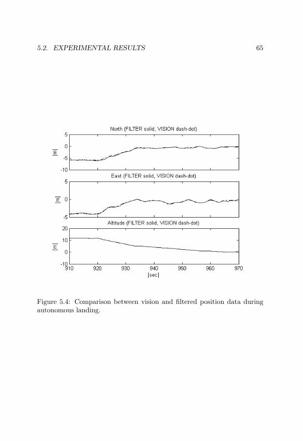
5.2. EXPERIMENTAL RESULTS 65
Figure 5.4: Comparison between vision and filtered position data duringautonomous landing.

66 CHAPTER 5. SENSOR FUSION FOR VISION BASED LANDING
noisy. Early attempts have been made in applying a low-pass filter to thisvelocity to remove the noise but the increased delay made the tuning of thecontrol system more difficult. The velocity data provided by the Kalmanfilter has low latency as can be observed from the comparison with the GPSvelocity. This is due to the fact that the Kalman filter takes advantage ofthe high frequency and low latency information from the accelerometers.The use of low latency velocity information allows for stable control duringthe landing approach.
Figure 5.5: Comparison between velocity derived from raw vision position,sensor fusion and GPS for the North component.
Figures 5.8 and 5.9, show a comparison between the attitude anglesprovided by the vision system alone (see Paper III for details as to how thevision system calculates the attitude angles), the attitude angles calculated

5.2. EXPERIMENTAL RESULTS 67
Figure 5.6: Comparison between velocity derived from raw vision position,sensor fusion and GPS for the East component.

68 CHAPTER 5. SENSOR FUSION FOR VISION BASED LANDING
Figure 5.7: Comparison between velocity derived from raw vision position,sensor fusion and GPS for the vertical component.

5.2. EXPERIMENTAL RESULTS 69
by the Kalman filter described in this chapter and the attitude given bythe YAS (attitude sensor built-in the RMAX helicopter). The attitudecalculated by the vision system alone suffers from bias errors and noisewhen compared to the YAS data. The reason for the bias is the mountingerror in angle between the camera platform and the helicopter body. Infact the camera is mounted on a suspended platform mounted on springsin order to damp helicopter vibrations and this produces alignment error.The angles given by the filter do not suffer from this problem and are ingood agreement with the YAS measurements.
Figure 5.8: Comparison between roll angle calculated by the vision system,sensor fusion and YAS.
Fig. 5.10 shows an altitude plot from a different landing test. One canobserve that when the helicopter was about 0.6 meters above the ground the

70 CHAPTER 5. SENSOR FUSION FOR VISION BASED LANDING
Figure 5.9: Comparison between pitch angle calculated by the vision sys-tem, sensor fusion and YAS.

5.3. CONCLUSION 71
vision system stopped delivering valid data because the pattern disappearedaccidentally out of the camera’s field of view. The filter continued to deliverposition information using its dead-reckoning capability until the landingwas terminated safely. This shows how sensor fusion techniques, enhancethe overall robustness of the landing procedure.
418 419 420 421 422 423 424 4250
0.2
0.4
0.6
0.8
1
altit
ude
[m]
time [s]
filterraw vision altitude
pattern occluded bythe shade of the helicopter
last valid vision measurement
touch down
Figure 5.10: Altitude plot of an autonomous landing completed with thevision lost before touch down.
5.3 Conclusion
In this chapter, the benefit of integrating inertial sensors with a visionsystem as part of a vision based autonomous landing system for an au-tonomous helicopter have been shown. The sensor fusion algorithm is basedon a Kalman filter where the inertial sensor errors are estimated using po-sition observation from a single camera vision system. The major benefitsin fusing inertial sensor with vision system can be summarized as resultingin a higher frequency state estimation, lower latency velocity estimation,more accurate attitude angle estimation and the possibility of survivingtemporary black-out in the vision system.

BIBLIOGRAPHY
Bibliography
[1] MARVIN: TU Berlin. http://pdv.cs.tu-berlin.de/MARVIN/.
[2] P. Doherty. Advanced Research with Autonomous Unmanned AerialVehicles. In Proc. of the Int. Conf. on the Principles of KnowledgeRepresentation and Reasoning, pages 731–732, 2004.
[3] P. Doherty, P. Haslum, F. Heintz, T. Merz, T. Persson, and B. Wing-man. A Distributed Architecture for Autonomous Unmanned AerialVehicle Experimentation. In Proc. of the Int. Symp. on DistributedAutonomous Robotic Systems, pages 221–230, 2004.
[4] S. Duranti and G. Conte. In-flight identification of the augmentedflight dynamics of the rmax unmanned helicopter. In Proc. of the 17thIFAC Symp. on Automatic Control in Aerospace, 2007.
[5] M. Egerstedt, X. Hu, and A. Stotsky. Control of mobile platformsusing a virtual vehicle approach. IEEE Transactions on AutomaticControl, 46(11):1777–1782, November 2001.
[6] M. Egerstedt, T. J. Koo, F. Hoffmann, and S. Sastry. Path planningand flight controller scheduling for an autonomous helicopter. LectureNotes in Computer Science, 1569:91–102, 1999.
[7] Bernard Etkin and Lloid Duff Reid. Dynamic of Flight: Stability andControl. John Wiley and Sons, Inc., 1995.
[8] J.A. Farrell and M. Barth. The Global Positioning System and InertialNavigation. McGraw-Hill, 1998.

BIBLIOGRAPHY 73
[9] E. Frazzoli. Robust Hybrid Control for Autonomous Vehicle MotionPlanning. PhD thesis, Massachusetts Institute of Technology, 2001.
[10] MIT/Draper Autonomous Helicopter Project.http://web.mit.edu/whall/www/heli/.
[11] Object Computing Inc. Tao developers guide, version 1.1a. 2000.
[12] R.E. Kalman. A new approach to linear filtering and prediction prob-lems. Transactions of the ASME-Journal of Basic Engineering, 82(Series D): 35-45, 1960.
[13] Jay Hyoun Kwon. Airborne Vector Gravimetry Using GPS/INS. Mas-ter Thesis, The Ohio State University, 2000.
[14] P Mantegazza et. al. RTAI: Real time application interface. LinuxJournal, 72, April 2000.
[15] T. Merz. Building a System for Autonomous Aerial Robotics Research.In Proc. of the IFAC Symp. on Intelligent Autonomous Vehicles, 2004.
[16] B. Mettler, M.B. Tischler, and T. Kanade. System identification ofsmall-size unmanned helicopter dynamics. American Helicopter Soci-ety 55th Annual Forum Proceedings, May 1999.
[17] Doherty P., Granlund G., Kuchcinski K., Sandewall E., Nordberg K.,Skarman E., and Wiklund J. The WITAS unmanned aerial vehicleproject. In Proc. of the European Conf. on Artificial Intelligence, pages747–755, 2000.
[18] P-O Pettersson. Using Randomized Algorithms for Helicopter PathPlanning. Linkoping, Sweden, 2006. Lic. Thesis Linkoping University.
[19] AVATAR: USC Autonomous Flying Vehicle Project. http://www-robotics.usc.edu/∼avatar.
[20] Raymond W. Prouty. Helicopter Performance, Stability and Control.Krieger Publishing Company, 1995.
74 BIBLIOGRAPHY
[21] D.F. Rogers and J.A. Adams. Mathematical Elements for ComputerGraphics. McGraw-Hill, 1990.
[22] R. T. Rysdyk. Uav path following for target observation in wind. Toappear in AIAA Journal of Guidance, Control, and Dynamics.
[23] Eun-Hwan Shin. Accuracy improvement of low cost INS/GPS for landapplications. Calgary, Alberta, 2001. Master Thesis, University ofCalgary.
[24] R. Skjetne and T. Fossen. Nonlinear maneuvering and control of ships.MTS/IEEE OCEANS 2001, 3:1808–15, 2001.
[25] Mattias Svensson. Aircraft Trajectory Restoration by Integration ofInertial Measurements and GPS. Master Thesis, Linkoping University,1999.
[26] Berkeley Aerorobot Team. http://robotics.eecs.berkeley.edu/bear/.
[27] Georgia Tech UAV. http://www.ae.gatech.edu/labs/controls/uavrf/.
[28] Hummingbird: Stanford University. http://sun-valley.stanford.edu/users/heli/.
[29] CMU Autonomous Helicopter Project.www.cs.cmu.edu/afs/cs/project/chopper/www.
[30] M. Wzorek and P. Doherty. Reconfigurable Path Planning for anAutonomous Unmanned Aerial Vehicle. In Proceedings of the Interna-tional Conference on Hybrid Information Technology, ICHIT, 2006.

75
Appendix A

76 APPENDIX A.
A.1 Paper I
DYNAMIC 3D PATH FOLLOWING FOR AN
AUTONOMOUS HELICOPTER
Gianpaolo Conte, 1 Simone Duranti, 1
Torsten Merz 1
Department of Computer and Information Science,Linkoping University, SE-58183 Linkoping, Sweden
Abstract: A hybrid control system for dynamic path following for an autonomoushelicopter is described. The hierarchically structured system combines continuouscontrol law execution with event-driven state machines. Trajectories are definedby a sequence of 3D path segments and velocity profiles, where each path segmentis described as a parametric curve. The method can be used in combination with apath planner for flying collision-free in a known environment. Experimental flighttest results are shown.
Keywords: aerospace engineering, architectures, autonomous vehicles, finite statemachines, helicopter control, splines, trajectories
1. INTRODUCTION
This work is part of the WITAS UnmannedAerial Vehicle (UAV) Project (Doherty, 2004),a long-term basic research project with the goalof developing information technology systems forUAVs and core functionalities necessary for theexecution of complex missions. The main objec-tive is the development of an integrated hard-ware/software UAV for fully autonomous missionsin an urban environment. A research prototypehas been developed using a Yamaha RMAX heli-copter as a flying platform. A number of interest-ing missions have been successfully demonstratedin a small uninhabited urban area in the southof Sweden called Revinge, which is used as anemergency services training area.
In order to navigate in an area cluttered byobstacles, such as an urban environment, pathplanning, path following (PF) and path switchingmechanisms are needed. Several methods have
1 Supported by the Wallenberg Foundation, Sweden
been proposed to solve this type of navigationproblem (Egerstedt et al., 1999; Frazzoli, 2001).
Our major achievements in this paper are thedevelopment and flight-testing of an algorithm tofollow a 3D path with a given velocity profile anda switching mechanism to enable the integrationwith a path planner in the deliberative part of theUAV architecture (Pettersson and Doherty, 2004).The method developed for PF is weakly model de-pendent and computationally efficient. The strat-egy used to follow a desired path is a velocitycontrol tangent to the path and a position controlorthogonal to it: the helicopter has to fly closeto the geometric path with a specified forwardspeed. This approach is better known as dynamicPF. In the trajectory tracking problem the systemis designed to follow a trajectory in the state-space domain where the state is parameterizedin time: the path is not prioritized. In PF meth-ods the path is always prioritized and this is arequirement for robots that for example have tofollow roads and avoid collisions with buildings. Atheoretical approach to dynamical PF is given in(Sarkar et al., 1994). The path we want to follow
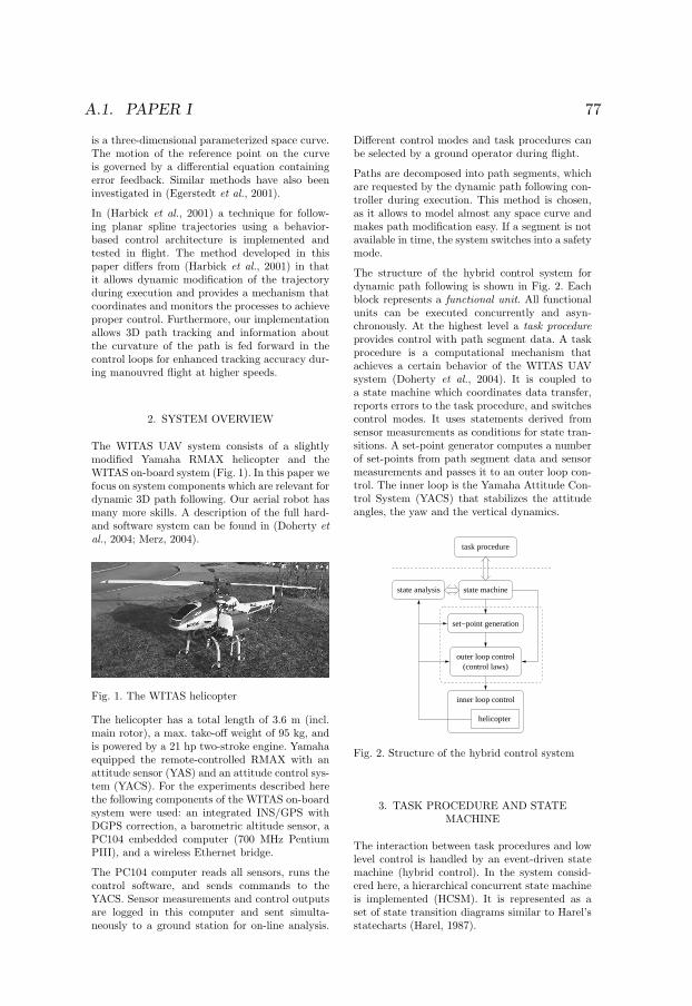
A.1. PAPER I 77
is a three-dimensional parameterized space curve.The motion of the reference point on the curveis governed by a differential equation containingerror feedback. Similar methods have also beeninvestigated in (Egerstedt et al., 2001).
In (Harbick et al., 2001) a technique for follow-ing planar spline trajectories using a behavior-based control architecture is implemented andtested in flight. The method developed in thispaper differs from (Harbick et al., 2001) in thatit allows dynamic modification of the trajectoryduring execution and provides a mechanism thatcoordinates and monitors the processes to achieveproper control. Furthermore, our implementationallows 3D path tracking and information aboutthe curvature of the path is fed forward in thecontrol loops for enhanced tracking accuracy dur-ing manouvred flight at higher speeds.
2. SYSTEM OVERVIEW
The WITAS UAV system consists of a slightlymodified Yamaha RMAX helicopter and theWITAS on-board system (Fig. 1). In this paper wefocus on system components which are relevant fordynamic 3D path following. Our aerial robot hasmany more skills. A description of the full hard-and software system can be found in (Doherty etal., 2004; Merz, 2004).
Fig. 1. The WITAS helicopter
The helicopter has a total length of 3.6 m (incl.main rotor), a max. take-off weight of 95 kg, andis powered by a 21 hp two-stroke engine. Yamahaequipped the remote-controlled RMAX with anattitude sensor (YAS) and an attitude control sys-tem (YACS). For the experiments described herethe following components of the WITAS on-boardsystem were used: an integrated INS/GPS withDGPS correction, a barometric altitude sensor, aPC104 embedded computer (700 MHz PentiumPIII), and a wireless Ethernet bridge.
The PC104 computer reads all sensors, runs thecontrol software, and sends commands to theYACS. Sensor measurements and control outputsare logged in this computer and sent simulta-neously to a ground station for on-line analysis.
Different control modes and task procedures canbe selected by a ground operator during flight.
Paths are decomposed into path segments, whichare requested by the dynamic path following con-troller during execution. This method is chosen,as it allows to model almost any space curve andmakes path modification easy. If a segment is notavailable in time, the system switches into a safetymode.
The structure of the hybrid control system fordynamic path following is shown in Fig. 2. Eachblock represents a functional unit. All functionalunits can be executed concurrently and asyn-chronously. At the highest level a task procedureprovides control with path segment data. A taskprocedure is a computational mechanism thatachieves a certain behavior of the WITAS UAVsystem (Doherty et al., 2004). It is coupled toa state machine which coordinates data transfer,reports errors to the task procedure, and switchescontrol modes. It uses statements derived fromsensor measurements as conditions for state tran-sitions. A set-point generator computes a numberof set-points from path segment data and sensormeasurements and passes it to an outer loop con-trol. The inner loop is the Yamaha Attitude Con-trol System (YACS) that stabilizes the attitudeangles, the yaw and the vertical dynamics.
task procedure
outer loop control(control laws)
state analysis
set−point generation
state machine
helicopter
inner loop control
Fig. 2. Structure of the hybrid control system
3. TASK PROCEDURE AND STATEMACHINE
The interaction between task procedures and lowlevel control is handled by an event-driven statemachine (hybrid control). In the system consid-ered here, a hierarchical concurrent state machineis implemented (HCSM). It is represented as aset of state transition diagrams similar to Harel’sstatecharts (Harel, 1987).

78 APPENDIX A.
braking controllerrunning
(single segment)controller running
dyn. path following
(multi segment)controller running
dyn. path following
(new seg. avail.)controller running
dyn. path following
DynPathMode
!#" $&%')(&*+,-.
/0%1120'3 4(6573809:,
: /4%11;3 '< /0%1120'3 0( ! =3 %
: ! %
! 3 > ?A@B1C1D
E F3 ; G! 3 > *+,-H ; G2I13 D HJ = 3' K MLON J = 3, K MPQN
! 3 > *+,-.H ; G2I13 D
; GR: %' H
Fig. 3. State machine for dynamic path following
In the following, the state machine for dynamicpath following is explained. The state transitiondiagram 2 is shown in Fig. 3. For a path withone segment (end velocity ve ≤ 0), the segmentparameters SegData are passed to the set-pointgenerator and the dynamic path following con-troller is started. A segment is defined by startand end points, start and end directions, targetvelocity, and end velocity. In the case of severalsegments (end velocity ve > 0), the state machinepasses the segment parameters, starts the samecontroller and sends a RequestSeg event to the taskprocedure. The next segment has to be providedbefore the helicopter reaches a point from whereit is impossible to stop at the end point of thecurrent segment (Close becomes true). This is asafety mechanism which prevents the helicopterfrom leaving the current path in case no new seg-ment is available. In this case, or if the helicopteris not able to slow down to the desired velocityat the end point, a SegError event is sent and abraking controller is started which will brake thehelicopter with maximum deceleration. When thehelicopter passes the end point of a path segment(Arrived becomes true) a Passed event is sent tothe task procedure. The state machine exits, whenthe helicopter hovers.
Fig. 4 shows an example of a state machine for apath with two segments 3. The upper part modelsa task procedure (user state machine) and thelower part a flight mode switching mechanism.Both machines run concurrently. When the au-tonomous mode is engaged (AutoSwitch becomestrue) the hovering controller is started. As soonas the helicopter hovers stably, the first segmentis flown. The hovering controller is started againwhen the helicopter arrives at the final waypoint.
2 Pulse is an event sent periodically, Init triggers a tran-
sition from an entry state (circular node) when condition
holds, Exit is sent to the superstate when entering an exit
state (square node).3 Rectangular boxes within state nodes denote nested
state machines. Superstate transitions are executed prior
to substate transitions.
finished
running (init)hovering controller
running (ready)hovering controller
second segment
first segment
1
2
dyn. path following
DynPathMode
SUTV,W'XYZ T [\IV,] VI^`_ aAb1c aAd c e b ce d cf1ghij klcf1ghij kl,mn
SUTopTq] Z T [YZ T [\IV,] VI^`_ a d c a#r c e d ce r cf1ghij klcs,mnkltuvwAx W_ yUz t) m
SUTVW'X
kltu SUTV,W,X
kltu v w ] |_ ~ lh n w p| |T] q m:p qT Up] Z# ] # Y
]
wAx W
# ] Y kltuvw ] |_ ~ lh n M1'T |\IV'] Vm n
p q1T7 I1'T| Z ] V, T Y
kltuvwAx W_ yUz t) m
kltu STV,W'X
Fig. 4. Example of a state machine for a path withtwo segments
In the real system, the state machine for modeswitching handles more flight modes and is sepa-rated from the user state machine (Merz, 2004).
4. SET-POINT GENERATION
The PF algorithm provides the set-points forthe outer loop control. The inputs are providedby the event handler and the position sensor(INS/DGPS).
The analytical description of the 3D path is acubic spline that has second-order continuity (C2)at the joints, this is a requirement which avoidsdiscontinuity in the helicopter’s acceleration. Aglobal reference frame is associated with eachsegment where the X-axis points north, the Y-axis points east and the Z-axis points down. Theanalytical form of the curve is:
P = As3 + Bs2 + Cs+ D (1)
where A, B, C and D are 3D vectors definedby the boundary conditions and s is the linearcoordinate of the curve.
For each value of s the path generator providesthe path parameters: position, tangent and cur-vature. The curvature is used to compute thecentripetal acceleration needed to follow the path(feed-forward term in the lateral control law),while the tangent T is used to align the helicopterbody to the path. The curvature K is a 3D vectorand is calculated in the global frame as follows:
K = T × Q × T /|T |4 (2)
T = 3As2 + 2Bs+ C (3)
Q = 6 As+ 2B (4)
where Q is the second order derivative.
A.1. PAPER I 79
The reference point on the nominal path is foundby satisfying the geometric condition that thescalar product between the tangent vector and theerror vector has to be zero:
E • T = 0 (5)
where the error vector E is the helicopter distancefrom the candidate control point. The controlpoint error feedback is then calculated as follows:
ef = E • T /|T | (6)
that is the magnitude of the error vector projectedon the tangent T . The control point is updatedusing the differential relation:
dP = P ′ · ds (7)
Equation 7 is applied in the discretized form:
s(n) = s(n− 1) +ef
|dP
ds(n− 1)|
(8)
where s(n) is the new value of the parameter.Once the new value of s is known, all the pathparameters can be calculated.
The PF algorithm receives as inputs the targetvelocity vt and the final velocity ve that the he-licopter must have at the end of the segment.The path planner assigns the target velocity whichis related to the mission specification only. Thismeans that the path planner doesn’t have to takeinto account any dynamic limitation of the he-licopter itself. The control law tries to keep thetarget velocity, but when it is not compatible withthe local curvature of the path and the helicopterperformance limitations, the algorithm providesan automatic limit on velocity. Velocity limita-tions can be activated for two reasons: due to theturn bank or the yaw rate limit of the helicopter.In order to make a coordinated turn at constantaltitude, the flight mechanics provides the relationbetween the velocity, the roll angle and the curva-ture radius of the turn. Mechanical limits exist onthe maximum achievable swash plate angles, andfurthermore the helicopter envelope has currentlybeen opened up to φmax±8 deg for the roll angle(relative to the hovering bank angle that is about4.5 deg), and ωmax±26 deg/sec for the yaw rate.Under the described limitations, it is possible tocalculate the maximum speed:
Vmax1 =√
Rgφmax (9)
Vmax2 = ω2
maxR (10)
where R is the local curvature radius and g is thegravity acceleration. The target speed assigned tothe path is compared with these two limits andthe lower speed is taken as target.
The braking algorithm continually checks the dis-tance between the helicopter and the end point ofthe path. If the required acceleration to reach the
final target velocity exceeds a given value (cur-rently set to 1 m/s2), the current target velocityis limited in order to maintain a constant deceler-ation. In order to know the distance between thehelicopter and the end of the path, an estimateof the final arc length of the curve has to becalculated. The arc length of the spline betweenthe control point and the end point of the path is:
lend =
∫ Send
S
√
[x′(s)]2
+ [y′(s)]2
+ [z′(s)]2ds
(11)If an analytical solution of the integral cannot befound, a numerical method is used (rectangularintegration with for example 20 integration steps).
To gain computational time, the increments of theflown path ln are subtracted from ltot (total lengthof the path, i.e. lend at first iteration) to get a goodestimate of lend at each control cycle:
ln =
√
√
√
√
√
[xn − xn−1]2
+
[yn − yn−1]2
+
[zn − zn−1]2
(12)
A path segment is considered finished when lend
is small enough. It should be emphasized that lend
is the arc length between the control point onthe curve and the end point of the path and notbetween the helicopter and the end of the path.This makes the system more robust with regardto position error of the helicopter on the path.
5. CONTROL LAWS
The outer loop control (velocity and positioncontrol) provides inputs for the YACS in orderto follow the path with the desired velocity. Theinner loop deals with the coupling dynamics ofthe helicopter, so that the outer loop can handlethe four degrees of freedom as decoupled (i.e.yaw rate, vertical velocity, pitch and roll angles).The position and velocity error and centripetalacceleration vectors are computed in the globalframe and then transformed into control inputsafter rotation in the helicopter’s body frame. Theacceleration vector is used as feed forward inputin the control law to improve the tracking inthe presence of path curvature. As regards theacceleration vector, only the component in thehorizontal plane orthogonal to the path is used.PD and PI compensators are used respectivelyfor position and velocity control. The algorithmdescribed in the previous section makes sure thatthe position error vector is orthogonal to thepath and the velocity error vector is tangent tothe path. Given that the two error vectors areorthogonal the velocity control doesn’t interferewith the position control. The control equationsfor the four channels are the following:

80 APPENDIX A.
θC =KpxδX +Kdx˙δX +KpvxδVX +
+KivxδVXsum +KfxAX
∆φC =KpyδY +Kdy˙δY +KpvyδVY +
+KivyδVY sum +KfyAY
VZC =KpzδZ +Kdz˙δZ +KpvzδVZ +
+KivzδVZsum +KfzAZ
ωC =Kpwδψ (13)
where the subscripted K’s are control gains, theδ′s are control errors, the pedices sum indicatethe integral terms and the A’s the componentsof the centripetal acceleration vector. θC is thetarget pitch angle, ∆φC is the desired roll anglerelative to the hovering roll angle, ωC is the targetyaw rate and VZC is the target vertical velocity.
6. EXPERIMENTAL RESULTS
The PF mode has been tested first in simulationand then in flight. The flight dynamics mathe-matical model of the augmented RMAX has beendeveloped within the WITAS project and imple-mented in C. Simulations are done using hardwarein the loop.Only results from the flights are reported in thefollowing.
−100
1020
3040
50
−100
−90
−80
−70−60
−50
−40
−30
−20
−100
0
10
20
30
40
50
60
East [m]
North [m]
Up
[m]
Flight TestTarget
A
B
Fig. 5. Target and actual 3D helicopter path
490 495 500 505 510 515 520 5250
2
4
6
8
10
12
Time [sec]
Spe
ed [m
/s]
flight testtarget
Fig. 6. Target and actual speed of the helicopter
Fig. 5 and 6 show a 3D segment and the velocityprofile during one of the flight-tests. The heli-copter hovers at point A at 40 meters altitude,
starts the descending spiral, brakes and hoversat point B at 10 meters altitude. The maximumspeed for the flight was set to 10 m/s, and the con-troller limited the target speed according to thelocal curvature and the braking algorithm. Themaximum vertical speed component was around3 m/s.
−60 −40 −20 0 20 40 60 80
−120
−100
−80
−60
−40
−20
East [m]
Nor
th [m
]
Flight TestTargetA
B C
D
Wind 5m/s
* *
Fig. 7. Multisegment 2D path
10 20 30 40 50 60 70 800
1
2
3
4
5
6
7
8
9
10
Time [sec]
Spe
ed [m
/s]
Flight TestTarget
A
B C
D
* *
*
*
Fig. 8. Speed profile of a multisegment path
Fig. 7 and 8 show a trajectory consisting of 3path segments at constant altitude. The missionstarts with autonomous hovering in point A, thenthe helicopter flies the first path segment withmaximum speed of 8 m/s; at point B the firstsegment is finished and a path switching leads thehelicopter to the second segment with a maximumspeed of 3 m/s; in point C the switch to the thirdpath segment with maximum speed of 8 m/s takesplace. Finally the helicopter brakes and hovers inpoint D where the mission ends. The wind wasblowing constantly at 5 m/s. The tracking errordepends on the angle between the path and thewind direction. In this case the maximum error isabout 3 meters.
Table 1 shows the results of several paths flownwith different wind conditions and different veloc-ities. The table reports three flight sessions (sepa-rated by horizontal lines) flown on three differentdays so as to cover three different wind conditions.In order to give more generality to the results,

A.1. PAPER I 81
Path Av Err Max Err St Dev Speed Wind
[-] [m] [m] [m] [m/s] [m/s]
HR 1.2 3.4 0.7 10 4
HL 1.9 4.1 1.3 10 4
DR 1.5 2.8 0.7 10 4
DL 1.8 3.5 1.1 10 4
CR 1.7 3.3 0.7 10 4
CL 1.9 4.1 1.3 10 4
HR 1.1 2.7 0.8 10 2
HL 0.8 2.2 0.6 10 2
DL 0.9 1.8 0.5 10 2
SLN 0.3 0.8 0.2 3 ≈ 0
SLN 0.5 1.4 0.3 3 ≈ 0
SLN 0.5 1.9 0.5 3 ≈ 0
SLN 0.6 1.4 0.3 3 ≈ 0
SLN 0.4 1.3 0.3 3 ≈ 0
HR = Horizontal Right HL = Horizontal Left
DR = Descending Right DL = Descending Left
CR = Climbing Right CL = Climbing Left
SLN = Straight Line
Table 1. Experimental data
representative paths of typical flight manoeuvreshave been chosen. In the HR path the helicopterdescribes a complete turn in the horizontal planeturning right, in the DR path the helicopter makesthe same turn while it is descending from 40 to 10meters and in the CR path the helicopter turnswhile climbing from 10 to 40 meters. The sameflights are repeated turning left instead. Fig. 5 forexample is a DL path.
The first column of the table shows the kindof path flown, the second, third and fourth col-umn are the average error, maximum error andstandard deviation error, and the fifth and sixthcolumn are the maximum ground speed reachedand the average wind speed. The error is thedistance of the helicopter to the reference pathand is calculated using the INS/GPS signal, whichis also used as control signal during flight (anindependent source would have been a better ref-erence for the purpose of this statistics). Becauseof the occurence of sudden jumps of the INS/GPSposition signal, the maximum errors shown in thetable are not always imputable to control errors;to evaluate the performance of the PF, the averageerror gives more reliable information.
To summarize the results of the table, the firstsession gives the worst results because of thewind, moreover the right turn gave better resultsthan the left one because the wind was blowingfrom the side. In the second session the overallperformance increases because of less wind. In thethird session several straight lines of 170 meters atlow speed were flown, during the test the wind wasnegligible.
7. CONCLUSIONS AND FUTURE WORK
The results of the experimentation show a sat-isfactory tracking behavior. The position control
error is well within the accuracy of the avail-able position measurement. The algorithm hasalso been successfully tested in relatively severeweather conditions, with wind levels up to 15 m/s.In the presence of the strongest wind levels, the al-gorithm could be improved in order to reduce thelateral error; an integrative compensator could beadded for this purpose but the tuning would notbe straight forward in presence of high curvature.The PF mode is now implemented in the softwarearchitecture of the WITAS helicopter and is beingused as a core functionality in complex missiontasks.
REFERENCES
Doherty et al. (2004). A distributed architec-ture for autonomous unmanned aerial vehi-cle experimentation. In: Proc. of the 7th In-ternational Symposium on Distributed Au-tonomous Robotic Systems. pp. 221–230.
Doherty, P. (2004). Advanced research with au-tonomous unmanned aerial vehicles. In: Proc.of the 9th International Conference on thePrinciples of Knowledge Representation andReasoning. pp. 731–732.
Egerstedt, M., T. J. Koo, F. Hoffmann and S. Sas-try (1999). Path planning and flight controllerscheduling for an autonomous helicopter. Lec-ture Notes in Computer Science 1569, 91–102.
Egerstedt, M., X. Hu and A. Stotsky (2001). Con-trol of mobile platforms using a virtual vehicleapproach. IEEE Transactions on AutomaticControl 46(11), 1777–1782.
Frazzoli, E. (2001). Robust Hybrid Control forAutonomous Vehicle Motion Planning. PhDthesis. Massachusetts Institute of Technology.
Harbick, K., J. Montgomery and G. Sukhatme(2001). Planar spline trajectory followingfor an autonomous helicopter. In: Proc. ofthe 2001 IEEE International Symposium onComputational Intelligence in Robotics andAutomation. pp. 408–413.
Harel, D. (1987). Statecharts: A visual formalismfor complex systems. Science of ComputerProgramming 8(3), 231–274.
Merz, T. (2004). Building a system for au-tonomous aerial robotics research. In: Proc. ofthe 5th IFAC Symposium on Intelligent Au-tonomous Vehicles.
Pettersson, P-O and P. Doherty (2004). Prob-abilistic roadmap based path planning foran autonomous unmanned aerial vehicle. In:ICAPS-04 Workshop on Connecting Plan-ning Theory with Practice.
Sarkar, N., X. Yun and V. Kumar (1994).Control of mechanical systems with rollingconstraints: Application to dynamic controlof mobile robots. International Journal ofRobotics Research (MIT Press) 13(1), 55–69.
82 APPENDIX A.
A.2 Paper II
From Motion Planning to Control - A Navigation Framework for an Autonomous Unmanned Aerial Vehicle
From Motion Planning to Control - A Navigation Frameworkfor an Autonomous Unmanned Aerial Vehicle
Mariusz Wzorek, Gianpaolo Conte, Piotr RudolTorsten Merz, Simone Duranti, Patrick Doherty
Department of Computer and Information ScienceLinkoping University, SE-58183 Linkoping, Swedenmarwz,giaco,pioru,g-torme,simdu,[email protected]
ABSTRACTThe use of Unmanned Aerial Vehicles (UAVs) which can operate autonomously in dynamic and complexoperational environments is becoming increasingly more common. While the application domains in which theyare currently used are still predominantly military in nature, in the future we can expect widespread usage in thecivil and commercial sectors. In order to insert such vehicles into commercial airspace, it is inherently importantthat these vehicles can generate collision-free motion plans and also be able to modify such plans during theirexecution in order to deal with contingencies which arise during the course of operation. In this paper, wepresent a fully deployed autonomous unmanned aerial vehicle, based on a Yamaha RMAX helicopter, whichis capable of navigation in urban environments. We describe a motion planning framework which integratestwo sample-based motion planning techniques, Probabilistic Roadmaps and Rapidly Exploring Random Treestogether with a path following controller that is used during path execution. Integrating deliberative services, suchas planners, seamlessly with control components in autonomous architectures is currently one of the major openproblems in robotics research. We show how the integration between the motion planning framework and thecontrol kernel is done in our system.
Additionally, we incorporate a dynamic path reconfigurability scheme. It offers a surprisingly efficient methodfor dynamic replanning of a motion plan based on unforeseen contingencies which may arise during the executionof a plan. Those contingencies can be inserted via ground operator/UAV interaction to dynamically change UAVflight paths on the fly. The system has been verified through simulation and in actual flight. We present empiricalresults of the performance of the framework and the path following controller.
BIOGRAPHYPatrick Doherty is a Professor at the Department of Computer and Information Science (IDA), LinkopingUniversity (LiU), Sweden. He is director of the Artificial Intelligence and Integrated Computer Systems Divisionat IDA and his research interests are in the area of knowledge representation, automated planning, autonomoussystems, approximate reasoning and UAV technologies.Mariusz Wzorek (MSc) is a graduate student at LiU. Research focus: automated planning techniques, autonomousunmanned systems and robotics.Gianpaolo Conte (MSc) is a graduate student at LiU. Research focus: control and sensor fusion related problems.Piotr Rudol (MSc) is a graduate student at LiU. Research focus: non-GPS navigation, mapping and obstacleavoidance for UAVs.Torsten Merz (PhD) has been involved in the WITAS project at LiU for many years. Since 2006, he is workingat the Autonomous Systems Lab at CSIRO (Australia) leading the development of an unmanned aerial vehicle forpower line inspection.Simone Duranti (MSc) is working at Saab Aerosystems and LiU. He has been involved in the WITAS project atLiU for many years.
21th Bristol UAV Systems Conference — April 2006

A.2. PAPER II 83
From Motion Planning to Control - A Navigation Framework for an Autonomous Unmanned Aerial Vehicle
1 Introduction
Navigating in environments cluttered with obstacles inthe vicinity of building structures requires path planningalgorithms which deliver collision-free paths, accuratecontrollers able to execute such paths even in thepresence of inhospitable weather conditions (e.g. windgusts) and a reliable mechanism that coordinates thetwo.
This paper describes an approach to combining pathplanning techniques with a path execution mechanism(including a robust 3D path following control mode)in a distributed software architecture used in a fullydeployed rotor-based Unmanned Aerial Vehicle (UAV).Details of many of the software components used inthe distributed architecture are provided. An emphasisis placed on the components responsible for pathexecution. The approach allows for interaction of a pathplanning algorithm with a path following control modeand copes with their different timing characteristicsand distributed communication. It also includes asafety mechanism which is necessary for operatingUAVs in urban environments. For the experimentswe present in this paper, we assume a predominantlystatic environment which is described by a 3D model.An onboard geographic information system (GIS) isused to supply information about building structures,vegetation, etc. Certain types of dynamic changes inthe environment are handled by the use of no-fly zonesor pop-up zones which can be added or removed on thefly during the course of a mission.
Our hardware/software framework incorporatessoftware distribution technologies for a numberof reasons. Firstly, existing commercial off-the-shelf(COTS) hardware suitable enough for airborne systems,does not yet have sufficient computational power andstorage space to encompass all the necessary softwarecomponents needed to achieve sophisticated missionscenarios autonomously. Additionally, in order touse third-party software without compromising flightsafety, it is necessary to separate software componentsthat can crash the operating system from software thatis crucial for the UAV flight operation. Another reasonfor using a distributed solution is to take advantageof additional resources which may be found on theInternet.
One of the long term goals which has guided ourresearch is the idea of push-button missions where theground operator supplies mission tasks to a UAV ata very high-level of abstraction and the UAV systemdoes most of the work ranging from planning to actual
execution of the mission.
The Autonomous UAV Technologies Laboratory 1 atLinkoping University, Sweden, has been developingfully autonomous rotor-based UAV systems in the mini-and micro-UAV class. Our current system design is theresult of an evolutionary process based on many yearsof developing, testing and maintaining sophisticatedUAV systems. In particular, we have used the YamahaRMAX helicopter platform and developed a number ofmicro air vehicles from scratch.
Much effort has also gone into the developmentof useful ground control station interfaces whichencourage the idea of push-button missions, lettingthe system itself plan and execute complex missionswith as little effort as possible required from theground operator other than stating mission goals at ahigh-level of abstraction and monitoring the executionof the ensuing mission. The mission scenarios weuse are generic in nature and may be instantiatedrelative to different applications. For example, thefunctionality required for the monitoring/surveillancemission described below can be modified slightly andused in mission scenarios such as power line inspection.
An example of such a push-button mission thathas been used as an application scenario in ourresearch is a combined monitoring/surveillance andphotogrammetry mission out in the field in an urbanarea with the goal of investigating facades of buildingstructures and gathering both video sequences andphotographs of building facades. For this experiment,we have used a Yamaha RMAX helicopter system as aplatform. Let us assume the operational environmentis in an urban area with a complex configurationof building and road structures. A number ofthese physical structures are of interest since one haspreviously observed suspicious behavior and suspectsthe possibility of terrorist activity. The goal of themission is to investigate a number of these buildings andacquire video and photos from each of the building’sfacades. It is assumed the UAV has a 3D model ofthe area and a GIS with building and road structureinformation on-line.
The ground operator would simply mark buildingstructures of interest on a map display and press a buttonto generate a complete multi-segment mission that fliesto each building, moves to waypoints to view eachfacade, positions the camera accordingly and beginsto relay video and/or photographs. The motion plansgenerated are also guaranteed to be collision-free from
1www.ida.liu.se/˜patdo/auttek/
21th Bristol UAV Systems Conference — April 2006
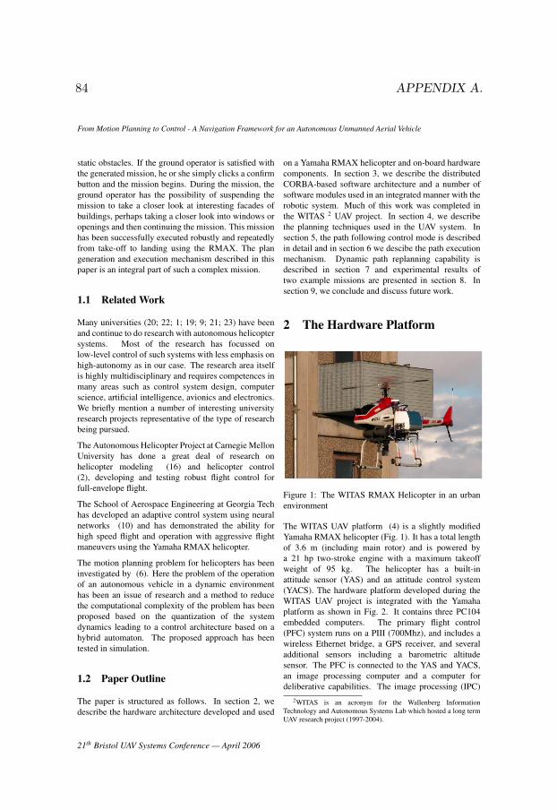
84 APPENDIX A.
From Motion Planning to Control - A Navigation Framework for an Autonomous Unmanned Aerial Vehicle
static obstacles. If the ground operator is satisfied withthe generated mission, he or she simply clicks a confirmbutton and the mission begins. During the mission, theground operator has the possibility of suspending themission to take a closer look at interesting facades ofbuildings, perhaps taking a closer look into windows oropenings and then continuing the mission. This missionhas been successfully executed robustly and repeatedlyfrom take-off to landing using the RMAX. The plangeneration and execution mechanism described in thispaper is an integral part of such a complex mission.
1.1 Related Work
Many universities (20; 22; 1; 19; 9; 21; 23) have beenand continue to do research with autonomous helicoptersystems. Most of the research has focussed onlow-level control of such systems with less emphasis onhigh-autonomy as in our case. The research area itselfis highly multidisciplinary and requires competences inmany areas such as control system design, computerscience, artificial intelligence, avionics and electronics.We briefly mention a number of interesting universityresearch projects representative of the type of researchbeing pursued.
The Autonomous Helicopter Project at Carnegie MellonUniversity has done a great deal of research onhelicopter modeling (16) and helicopter control(2), developing and testing robust flight control forfull-envelope flight.
The School of Aerospace Engineering at Georgia Techhas developed an adaptive control system using neuralnetworks (10) and has demonstrated the ability forhigh speed flight and operation with aggressive flightmaneuvers using the Yamaha RMAX helicopter.
The motion planning problem for helicopters has beeninvestigated by (6). Here the problem of the operationof an autonomous vehicle in a dynamic environmenthas been an issue of research and a method to reducethe computational complexity of the problem has beenproposed based on the quantization of the systemdynamics leading to a control architecture based on ahybrid automaton. The proposed approach has beentested in simulation.
1.2 Paper Outline
The paper is structured as follows. In section 2, wedescribe the hardware architecture developed and used
on a Yamaha RMAX helicopter and on-board hardwarecomponents. In section 3, we describe the distributedCORBA-based software architecture and a number ofsoftware modules used in an integrated manner with therobotic system. Much of this work was completed inthe WITAS 2 UAV project. In section 4, we describethe planning techniques used in the UAV system. Insection 5, the path following control mode is describedin detail and in section 6 we descibe the path executionmechanism. Dynamic path replanning capability isdescribed in section 7 and experimental results oftwo example missions are presented in section 8. Insection 9, we conclude and discuss future work.
2 The Hardware Platform
Figure 1: The WITAS RMAX Helicopter in an urbanenvironment
The WITAS UAV platform (4) is a slightly modifiedYamaha RMAX helicopter (Fig. 1). It has a total lengthof 3.6 m (including main rotor) and is powered bya 21 hp two-stroke engine with a maximum takeoffweight of 95 kg. The helicopter has a built-inattitude sensor (YAS) and an attitude control system(YACS). The hardware platform developed during theWITAS UAV project is integrated with the Yamahaplatform as shown in Fig. 2. It contains three PC104embedded computers. The primary flight control(PFC) system runs on a PIII (700Mhz), and includes awireless Ethernet bridge, a GPS receiver, and severaladditional sensors including a barometric altitudesensor. The PFC is connected to the YAS and YACS,an image processing computer and a computer fordeliberative capabilities. The image processing (IPC)
2WITAS is an acronym for the Wallenberg InformationTechnology and Autonomous Systems Lab which hosted a long termUAV research project (1997-2004).
21th Bristol UAV Systems Conference — April 2006

A.2. PAPER II 85
From Motion Planning to Control - A Navigation Framework for an Autonomous Unmanned Aerial Vehicle
system runs on the second PC104 embedded computer(PIII 700MHz), and includes a color CCD cameramounted on a pan/tilt unit, a video transmitter anda recorder (miniDV). The deliberative/reactive (DRC)system runs on the third PC104 embedded computer(Pentium-M 1.4GHz) and executes all high-endautonomous functionality. Network communicationbetween computers is physically realized with serialline RS232C and Ethernet. Ethernet is mainly used forCORBA applications (see below), remote login and filetransfer, while serial lines are used for hard real-timenetworking.
DRC - 1.4 GHz P-M - 1GB RAM - 512 MB flash
IPC - 700 MHz PIII - 256MB RAM - 512 MB flash
Yamaha RMAX (YAS, YACS)
ethernetswitch
PFC - 700 MHz PIII - 256MB RAM - 512 MB flash
sensor suite
sensorsuite
RS232C Ethernet Other media
Figure 2: On-board hardware schematic
3 The Software Architecture
A hybrid deliberative/reactive software architecture hasbeen developed for the UAV. Conceptually, it is alayered, hierarchical system with deliberative, reactiveand control components, although the system can easilysupport both vertical and horizontal data and controlflow. Fig. 3 presents the functional layer structure ofthe architecture and emphasizes its reactive-concentricnature. Fig. 4 depicts the navigation subsystem andmain software components. With respect to timingcharacteristics, the architecture can be divided into twolayers: (a) the hard real-time part, which mostly dealswith hardware and control laws (also referred to asthe Control Kernel) and (b) the non real-time part,which includes deliberative services of the system (alsoreferred to as the High-level system) 3. All three
3Note that distinction between the Control Kernel and theHigh-level system is done based mainly on the timing characterisitcsand it does not exclude, for example, placing some deliberative
Figure 3: Funcional structure of the architecture
computers in our UAV platform (i.e. PFC, IPC andDRC) have both hard and soft real-time componentsbut the processor time is assigned to them in differentproportions. On one extreme, the PFC runs mostlyhard real-time tasks with only minimum user spaceapplications (e.g. SSH daemon for remote login). Onthe other extreme, the DRC uses the real-time partonly for device drivers and real-time communication.The majority of processor time is spent on runningthe deliberative services. Among others, the mostimportant ones from the perspective of this paper are thePath Planner, the Task Procedure Execution Module andthe Helicopter Server which encapsulates the ControlKernel (CK) of the UAV system.
The CK is a distributed real-time runtime environmentand is used for accessing the hardware, implementingcontinuous control laws, and control mode switching.Moreover, the CK coordinates the real-timecommunication between all three on-board computersas well as between CKs of other robotic systems. Inour case, we perform multi-platform missions withtwo identical RMAX helicopter platforms developedin the WITAS UAV project. The CK is implementedusing C language. This part of the system uses theReal-Time Application Interface (RTAI) (13) whichprovides industrial-grade real-time operating systemfunctionality. RTAI is a hard real-time extension to astandard Linux kernel (Debian in our case) and hasbeen developed at the Department of the AerospaceEngineering of Politecnico di Milano.
The real-time performance is achieved by inserting
services (e.g. prediction) in the Control Kernel.
21th Bristol UAV Systems Conference — April 2006

86 APPENDIX A.
From Motion Planning to Control - A Navigation Framework for an Autonomous Unmanned Aerial Vehicle
Task Procedures*
HCSMInterpreter
OtherModes
Communi-cation
Handling
PFC
DRC
Real-timecommunication channel
Path PlannerService*
Helicopter Server*
CORBAHCSM Interpreter (C-API)
GISService*
OtherServices*
HardwareHandling
Path Following
Mode
HoveringMode
DistributedSystem*- CORBA-based
Figure 4: Navigation subsystem and main softwarecomponents
a module into the Linux kernel space. Since themodule takes full control over the processor it isnecessary to suspend it in order to let the user spaceapplications run. The standard Linux distribution is atask with lower priority, it runs preemptively and canbe interrupted at any time. For that reason a lockingmechanism is used when both user- and kernel-spaceprocesses communicate though shared memory. It isalso important to mention that the CK is self-containedand only the part running on the PFC computer isnecessary for maintaining flight capabilities. Suchseparation enhances safety of the operation of theUAV platform which is especially important in urbanenvironments.
The Control Kernel has a hybrid flavor. Its componentscontain continuous control laws and mode switching isrealized using event-driven hierarchical concurrent statemachines (HCSMs). They can be represented as statetransition diagrams similar to those of statecharts (8).In our system, tables describing transitions derived fromsuch diagrams are passed to the system in the form oftext files and are interpreted by a HCSM Interpreter atrun-time in each of the on-board computers. Thanks toits compact and efficient implementation, the interpreterruns in the real-time part of the system as a task withhigh execution rate. It allows coordinating all functional
units of the control system from the lowest levelhardware components (e.g. device drivers) throughcontrol laws (e.g. hovering, path following) andcommunication to the interface used by the HelicopterServer.
The use of HCSMs also allows implementing complexbehaviors consisting of other lower level ones. Forinstance, landing mode includes control laws steeringthe helicopter and coordinates camera system/imageprocessing functionalities. When the landing behavioris activated, the CK takes care of searching for apre-defined pattern with the camera system, feedingthe Kalman filter with image processing results whichfuses them with the helicopter’s inertial measurements.The CK sends appropriate feedback when the landingprocedure is finished or it has been aborted. For detailssee (15).
For achieving best performance, a singlenon-preemptive real-time task is used which follows apredefined static schedule to run all functional units.Similarly, the real-time communication physicallyrealized using serial lines is statically scheduled withrespect to packet sizes and rates of sending. For adetailed description see (14).
The high-level part of the system has reduced timingrequirements and is responsible for coordinating theexecution of reactive Task Procedures (TPs). Thispart of the system uses Common Object RequestBroker Architecture (CORBA) as its distributionbackbone. A TP is a high-level procedural executioncomponent which provides a computational mechanismfor achieving different robotic behaviors by usingboth deliberative and control components in a highlydistributed and concurrent manner. The control andsensing components of the system are accessible forTPs through the Helicopter Server which in turn usesan interface provided by the Control Kernel. A TPcan initiate one of the autonomous control flight modesavailable in the UAV (i.e. take off, vision-based landing,hovering, dynamic path following (see section 5) orreactive flight modes for interception and tracking).Additionally, TPs can control the payload of theUAV platform which currently consists of the videocamera mounted on a pan-tilt unit. TPs receivedata delivered by the PFC and IPC computers i.e.helicopter state and camera system state (includingimage processing results), respectively. The HelicopterServer on one side uses CORBA to be accessible by TPsor other components of the system, on the other side itcommunicates through shared memory with the HCSMbased interface running in the real-time part of the DRC
21th Bristol UAV Systems Conference — April 2006

A.2. PAPER II 87
From Motion Planning to Control - A Navigation Framework for an Autonomous Unmanned Aerial Vehicle
software.
The software architecture described is used to achievemissions which require deliberative services such aspath planners and control laws such as path followingdescribed in detail in sections 4 and 5, respectively.Details of the interaction between the TPs, pathplanners and the Control Kernel are presented in section6.
4 The Path Planning Algorithms
In this section, we provide a brief overview of thesample-based path planning techniques used in ourframework. More detailed descriptions of the two pathplanners can be found in (18; 17).
The problem of finding optimal paths between twoconfigurations in a high-dimensional configurationspace such as a helicopter is intractable in general.Sample-based approaches such as probabilisticroadmaps (PRM) or rapidly exploring random trees(RRT) often make the path planning problem solvablein practice by sacrificing completeness and optimality.
4.1 Probabilistic Roadmaps
The standard probabilistic roadmap (PRM) algorithm(11) works in two phases, one off-line and theother on-line. In the off-line phase a roadmap isgenerated using a 3D world model. Configurationsare randomly generated and checked for collisionswith the model. A local path planner is then usedto connect collision-free configurations taking intoaccount kinematic and dynamic constraints of thehelicopter. Paths between two configurations are alsochecked for collisions. In the on-line or queryingphase, initial and goal configurations are provided andan attempt is made to connect each configuration tothe previously generated roadmap using the local pathplanner. A graph search algorithm such as A∗ isthen used to find a path from the initial to the goalconfiguration in the augmented roadmap.
Fig. 5 provides a schema of the PRM path plannerused in the WITAS UAV system. The planner uses anOBBTree-algorithm (7) for collision checking and anA∗ algorithm for graph search. Here one can optimizefor shortest path, minimal fuel usage, etc. The followingextensions have been made with respect to the standardversion of the PRM algorithm in order to adapt theapproach to our UAV platform.
Figure 5: PRM path plan generation
• Multi-level roadmap planning
The standard probabilistic roadmap algorithm isformulated for fully controllable systems only.This assumption is true for a helicopter flying atlow speed with the capability to stop and hoverat each waypoint. However, when the speedis increased the helicopter is no longer able tonegotiate turns of a smaller radius, which imposesdemands on the planner similar to non-holonomicconstraints for car-like robots. In this case, linearpaths are first used to connect configurations inthe graph and at a later stage these are replacedwith cubic curves when possible. These arerequired for smooth high speed flight. If it isnot possible to replace a linear path segmentwith a cubic curve then the helicopter has toslow down and switch to hovering mode at theconnecting waypoint before continuing. Fromour experience, this rarely happens.
• Runtime constraint handling
Our motion planner has been extended to dealwith different types of constraints at runtime notavailable during roadmap construction. Suchconstraints can be introduced at the time ofa query for a path plan. Some examplesof runtime constraints currently implementedinclude maximum and minimum altitude, addingforbidden regions (no-fly zones) and placinglimits on the ascent-/descent-rate. Suchconstraints are dealt with during the A∗ searchphase.
The mean planning time in the current implementation(for our operational environments) is below 1000 msand the use of runtime constraints do not noticeablyinfluence the mean.
21th Bristol UAV Systems Conference — April 2006

88 APPENDIX A.
From Motion Planning to Control - A Navigation Framework for an Autonomous Unmanned Aerial Vehicle
4.2 Rapidly Exploring Random Trees
The use of rapidly exploring random trees (RRT)provides an efficient motion planning algorithm thatconstructs a roadmap online rather than offline. Thealgorithm (12) generates two trees rooted in the startand end configurations by exploring the configurationspace randomly in both directions. While the trees arebeing generated, an attempt is made at specific intervalsto connect them to create one roadmap. After theroadmap is created, the remaining steps in the algorithmare the same as with PRMs. In comparison with thePRM planner, the mean planning time with RRT is alsobelow 1000 ms, but in this case, the success rate ismuch lower and the generated plans are not optimalwhich may sometimes cause anomalous detours (17).
Results of the path planning algorithms are used bythe path following controller described in the followingsection.
5 Path Following Control Mode
In this section, we provide a detailed description of apath following control mode (Fig. 6, the bottom part ofFig. 4) which executes paths provided by the plannerintroduced in section 4. As described in section 3,the HCSM-based Control Kernel coordinates executionof different control modes available in the UAV system,including the path following control mode.
In the classical approach to the trajectory followingproblem, a trajectory is generated directly taking intoaccount the dynamic constraints of the system. Inour approach, however, we split the problem into twoparts. First, the path planner generates a geometricaldescription of a path and the dynamic constraints arehandled later by the path following mode by generatingan appropriate velocity profile. In order to navigatesafely in urban environments, the path following modehas been designed to minimize the tracking error duringa path execution. Because paths generated by theplanner are collision-free (relative to the static obstaclespresent in the model), staying closer to the geometricpath assures safer navigation in the environment.
A path is composed of one or more segments (eachdescribed by a 3D cubic curve) which are passedsequentially to the control mode. The mode isimplemented as a function which takes as inputthe segment geometry, the desired cruise and finalvelocities. It is called by the Control Kernel with
HCSMInterpreter
Trajectorygenerator
Path controller(Outer control loop)
Inner control loop (YACS)
Helicopter platform
Path FollowingControl Mode
Figure 6: Interaction between the Path FollowingControl Mode and other components of the ControlKernel
a frequency of 50Hz and its output consists of fourcontrol signals (pitch, roll, yaw and the verticalchannel). Additionally, the function returns a set ofstatus flags which are used by the HCSM in control togenerate appropriate events, i.e. path segment switchingmechanism and safety braking procedure.
When the helicopter reaches the end point of the currentsegment, the controlling HCSM is informed and anArrived event is generated. The next call to the pathfollowing function is made using parameters describingthe next segment to be flown. The process continuesuntil all segments of the path are executed.
The safety braking procedure is activated in case thenext segment is not provided by the High-level system(e.g. due to communication failure) in a specific time.This time point is calculated as the minimum distancenecessary to stop the helicopter at the end of the currentsegment without overshooting.
The path tracking error is also available to thecontrolling HCSM and it can be used to take appropriateactions in case it becomes too large to guarantee safeoperation. Such a situation can arise if the wind is toostrong for the platform to keep it on the desired path.
The path following control mode is conceptuallydivided into two parts: (a) the Trajectory Generator(TG) which calculates the reference trajectory used by(b) the Path Controller (PC) to calculate the controlsignals. We consider each part in the next twosubsections.
21th Bristol UAV Systems Conference — April 2006

A.2. PAPER II 89
From Motion Planning to Control - A Navigation Framework for an Autonomous Unmanned Aerial Vehicle
5.1 Trajectory Generator
A trajectory represents the evolution of a dynamicsystem in the state-space domain, where the statevariables are parameterized in time. In our approachthe generated reference trajectory (based on the planneroutput) depends not on the time but on the position ofthe helicopter relative to the path. In order to calculatethe reference trajectory, a control point on the pathwhich is the closest to the helicopter position must befound. Once this is done, the trajectory parameterscan be calculated and used by the path controller(described in the next subsection) as set-points. Afeedback method is used to find the control point,similar approach is used in (5).
The reference trajectory in this work is a vectorrepresented by 9 components: x(s), y(s) and z(s)represent the respective East, North positions andaltitude of the helicopter relative to an initial point;vx(s), vy(s) and vz(s) the North, East and verticalvelocity components; φ(s), θ(s) and ψ(s) the roll,pitch and yaw angles; s is the path segment parameter.Details of the calculation of the parameter s throughfeedback can be found in (3).
The geometric path is composed of several segmentsrepresented by a 3D cubic polynomial. The motivationfor using this type of curve is given in (17). A3D geometric segment is represented by the followingequation in a vector form:
P (s) = As3 + Bs2 + Cs+ D
where A, B, C and D are 3D vectors defined by theboundary conditions calculated by the path planner andpassed to the control mode, s=[0,1] is the parameter ofthe curve and P = [x, y, z]. 0nce the parameter s isfound the position coordinates x, y, z can be calculated.
In order to achieve the necessary tracking performance,the path curvature is fed forward in the roll control law.The target roll angle value is calculated according to thefollowing formula:
φ(s) =V 2
Rxy(s)g
where V is the helicopter speed, g is the gravityacceleration and Rxy(s) is the local curvature radiusof the path projected on the horizontal plane. Thecurvature radius of the path is a 3D vector and it iscalculated analytically as explained in (3).
The same approach could be applied in order tocalculate the target pitch angle θ(s). However, for
the helicopter flight envelope we are interested in, thedynamics of the path curvature in the vertical directionis not very fast. Therefore, the feed forward term is notused for the pitch channel.
The yaw angle ψ(s) is calculated from the tangentvector of the path. The tangent is projected on thehorizontal (East-North) plane and used as referencesignal for the yaw control.
The target path velocity (Vtar(s)) is derived fromtwo input parameters: the cruise velocity Vc (desiredvelocity for the segment) and the final velocity Vf
(velocity that the helicopter must have at the end ofthe segment). Both velocities are given by the pathplanners.
The calculation of Vtar(s) along the path segment isdivided into three phases: acceleration, cruise andbraking. The acceleration phase is active only duringexecution of the first segment of the path. During thisphase the velocity increases with a constant rate untilthe cruise velocity Vc is reached. Note that in this caseVtar depends on time rather than on the path parameter(s) since it is not important at which position of the paththe acceleration phase is terminated.
The braking phase is active when the followingcondition is satisfied: the remaining path length dend(s)is equal to the distance required to brake the helicopterfrom Vc to Vf for given deceleration abrake:
dend(s) =|V 2
c − V 2f |
2abrake
The target velocity in the braking phase is a function ofdend(s):
Vtar(s) =√|2dend(s)abrake + V 2
f |
This guarantees achieving the desired velocity at theend of the path segment. In case Vf > Vc, thehelicopter accelerates in order to reach Vf at the endof the path segment. The path planner assures thecontinuity of the velocity profile between segments. Inorder to make a coordinated turn a consistency checkmust be done with respect to the generated Vtar(s).For such a maneuver, the helicopter must compensatethe centripetal acceleration with a certain amount ofroll angle. Because of safety reasons the maximumroll angle (φmax) and maximum yaw rate (ωmax) arespecified. Therefore, the maximum velocity during aturn maneuver is also restricted. The two velocity limits
21th Bristol UAV Systems Conference — April 2006

90 APPENDIX A.
From Motion Planning to Control - A Navigation Framework for an Autonomous Unmanned Aerial Vehicle
−20 0 20 40 60 80
−180
−160
−140
−120
−100
−80
−60
−40
−20
0
20
East [m]
Nor
th [m
]
Closed loop YACS on the roll channel
Flight testedTarget
−20 0 20 40 60 80
−180
−160
−140
−120
−100
−80
−60
−40
−20
0
20
East [m]
Nor
th [m
]
Open loop YACS
Flight testedTarget
Start End
Start End
Figure 7: Comparison of path tracking performances using two different roll controller. The flight-test whereperformed at 36 km/h constant velocity for both paths.
are calculated as follows:
Vmax1(s) =√Rxy(s)gφmax
Vmax2(s) = ω2maxRxy(s)
The minimum between Vmax1(s), Vmax2(s) andVtar(s) is taken as target velocity by the path controllerdescribed in the next subsection. Thus, the calculatedvelocity is compatible with the curvature radius of thepath.
5.2 Path Controller
Usually the control system for a helicopter consists ofan inner loop, which is responsible for stabilizing theattitude, and the outer loop, which controls the positionand velocity.
In our system we use the Yamaha Attitude ControlSystem (YACS) provided with the RMAX helicopterfor the attitude control. For the outer loop we use fourdecoupled PID controllers. Their outputs are used asinput to the YACS system. In (3) the control approachfor the RMAX has been described and experimentalresults provided.
In this section, we present results of a modifiedcontroller, which uses an additional feedback loop on
the roll channel. Several experiments were done closingthe roll angle loop around the YACS in order to test if itis feasible to improve path tracking precision without acomplete redesign of the attitude controller.
The modified controller has been flight-tested on theRMAX helicopter at a constant velocity of 36km/hon a path with changing curvature. Such a pathis typically used to navigate in areas with obstacles.The results are shown in Fig. 7 where the same pathwas tested both with the roll loop closed around theYACS, and without. Note, that at the beginning ofthe path when the dynamic response of the controlleris more important because of the changing curvature,the control with additional feedback loop over theroll channel performs much better than the other one.The error for the closed loop controller in this partis below 1 meter, while for the other is around 6meters. The results obtained during flight-tests showthat the loop on the roll channel reduces the pathtracking error, what makes the controller more suitablefor obstacle-cluttered environments.
The following section describes interaction between thepath following control mode with a Task Procedureresponsible for executing a planned path.
21th Bristol UAV Systems Conference — April 2006
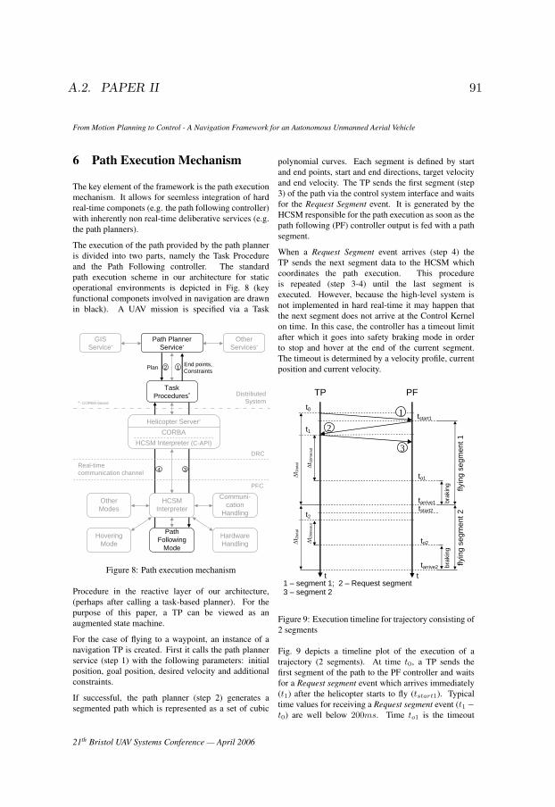
A.2. PAPER II 91
From Motion Planning to Control - A Navigation Framework for an Autonomous Unmanned Aerial Vehicle
6 Path Execution Mechanism
The key element of the framework is the path executionmechanism. It allows for seemless integration of hardreal-time componets (e.g. the path following controller)with inherently non real-time deliberative services (e.g.the path planners).
The execution of the path provided by the path planneris divided into two parts, namely the Task Procedureand the Path Following controller. The standardpath execution scheme in our architecture for staticoperational environments is depicted in Fig. 8 (keyfunctional componets involved in navigation are drawnin black). A UAV mission is specified via a Task
Plan 2 1
Task Procedures*
End points,Constraints
34
HCSMInterpreter
OtherModes
Communi-cation
Handling
PFC
DRC
Real-timecommunication channel
Path PlannerService*
Helicopter Server*
CORBAHCSM Interpreter (C-API)
GISService*
OtherServices*
HardwareHandling
Path Following
Mode
HoveringMode
DistributedSystem*- CORBA-based
Figure 8: Path execution mechanism
Procedure in the reactive layer of our architecture,(perhaps after calling a task-based planner). For thepurpose of this paper, a TP can be viewed as anaugmented state machine.
For the case of flying to a waypoint, an instance of anavigation TP is created. First it calls the path plannerservice (step 1) with the following parameters: initialposition, goal position, desired velocity and additionalconstraints.
If successful, the path planner (step 2) generates asegmented path which is represented as a set of cubic
polynomial curves. Each segment is defined by startand end points, start and end directions, target velocityand end velocity. The TP sends the first segment (step3) of the path via the control system interface and waitsfor the Request Segment event. It is generated by theHCSM responsible for the path execution as soon as thepath following (PF) controller output is fed with a pathsegment.
When a Request Segment event arrives (step 4) theTP sends the next segment data to the HCSM whichcoordinates the path execution. This procedureis repeated (step 3-4) until the last segment isexecuted. However, because the high-level system isnot implemented in hard real-time it may happen thatthe next segment does not arrive at the Control Kernelon time. In this case, the controller has a timeout limitafter which it goes into safety braking mode in orderto stop and hover at the end of the current segment.The timeout is determined by a velocity profile, currentposition and current velocity.
∆t2t
imeo
ut
∆t1t
otal
∆t1t
imeo
ut
brak
ing flyin
g se
gmen
t 1
TP t0
PF
tstart1
to1
tarrive1
t1
brak
ing
flyin
g se
gmen
t 2
to2
tarrive2
1
2
3
t t 1 – segment 1; 2 – Request segment 3 – segment 2
tstart2 t2
∆t2t
otal
Figure 9: Execution timeline for trajectory consisting of2 segments
Fig. 9 depicts a timeline plot of the execution of atrajectory (2 segments). At time t0, a TP sends thefirst segment of the path to the PF controller and waitsfor a Request segment event which arrives immediately(t1) after the helicopter starts to fly (tstart1). Typicaltime values for receiving a Request segment event (t1 −t0) are well below 200ms. Time to1 is the timeout
21th Bristol UAV Systems Conference — April 2006

92 APPENDIX A.
From Motion Planning to Control - A Navigation Framework for an Autonomous Unmanned Aerial Vehicle
for the first segment which means that the TP has a∆t1timeout time window to send the next segment tothe PF controller before it initiates a safety brakingprocedure. If the segment is sent after to1, the helicopterwill start braking. In the current implementation,segments are not allowed to be sent after a timeout.This will be changed in a future implementation. Inpractice, the ∆t1timeout time window is large enoughto replan the path using the standard path planner. Theupdated segments are then sent to the PF controllertransparently.
The described path execution mechanism allows fordynamic replacement of path segments if necessary.The following section describes the process of dynamicpath replanning.
Init Align
Send segment
Exit
Plan
not al
igned
alig
ned
last
segment
sent
no-f
ly z
one
upda
ted
request segmentreceived
Estimate timeout
timeo
ut
calc
ulat
ed
Check collision
Replan
Wait
timeout conditionupdated path
no c
ollis
ion
StrategySelection
TimesEstimation
StrategyLibrary
collision detectedstra
tegy
que
ry
stra
tegy
path
plan path with strategy
path
estim
ated t
iming
sest
imate
timing
s
for se
gmen
ts
Static
plan
pat
h
Figure 10: The dynamic path replanning automaton
7 Dynamic Replanning of the Path
The design of the path execution mechanism providesa method for feeding path segments to the PFcontroller iteratively. This is a particularly interestingpart of the design because it gives the deliberativeor decision-making layer of the architecture theopportunity to anticipate problems at longer temporalhorizons and then to modify one or more segmentsin the original mission path plan based on anycontingencies it discovers.
There are several services that are used during the pathreplanning stage. They are called when changes inthe environment are detected and an update event isgenerated in the system. The augmented state machineassociated with the TP used for the dynamic replanningof a path is depicted in Fig. 10. The TP takes a start andan end point and a target velocity as input. The TP thencalls a path planning service (Plan state) which returnsan initial path.
If the helicopter is not aligned with the direction ofthe flight, a command to align is sent to the controller(Align state).The TP then sends the first segment of thegenerated path to the PF controller (Send segment state)and calls the Prediction service to estimate a timeoutfor the current segment (Estimate timeout state). Basedon the segment timeout and system latency, a conditionis calculated for sending the next segment. If there isno change in the environment the TP waits (Wait state)until a timeout condition is true and then sends the nextsegment to the PF controller.
In case new information about newly added or deletedforbidden regions (no-fly zone updated) arrives, the TPchecks if the current path is in collision with the updatedworld model (Check Collision state). If a collision isdetected in one or more segments the TP calls a StrategySelector service (Strategy Selection state) to determinewhich replanning strategy is the most appropriate touse at the time. The Strategy Selector service uses thePrediction service for path timings estimation (TimesEstimation state) to get estimated timeouts, total traveltimes etc. It also uses the Strategy Library service(Strategy Library state) to get available replanningstrategies that will be used to replan when calling thepath planner (Replan state). The TP terminates whenthe last segment is sent.
All time estimations that have to do with paths or partsof paths are handled by the Prediction service. It usesthe velocity profile of a vehicle and path parametersto calculate timeouts, total times, and combinations ofthose. For instance, in the case of flying a two-segmenttrajectory (see execution timeline in Fig. 9) it canestimate timeouts (∆t1timeout, ∆t2timeout), total traveltimes (∆t1total, ∆t2total) as well as a combined timeoutfor the first and the second segment (to2-t1).
When part of a path is not valid anymore, the pathplanner service can be called in order to repair anexisting plan or to create a new one. There are manystrategies that can be used at that step which cangive different results depending on the situation. TheStrategy Library stores different replanning strategiesincluding information about the replanning algorithm to
21th Bristol UAV Systems Conference — April 2006
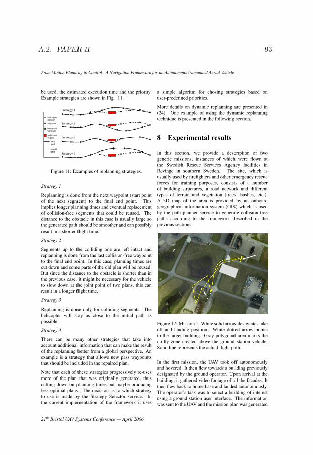
A.2. PAPER II 93
From Motion Planning to Control - A Navigation Framework for an Autonomous Unmanned Aerial Vehicle
be used, the estimated execution time and the priority.Example strategies are shown in Fig. 11.
helicopter position waypoint
forbidden region
final path
invalid path
Strategy 1
Strategy 2
Strategy 3
Strategy 4
new pass waypoint
Figure 11: Examples of replanning strategies.
Strategy 1
Replanning is done from the next waypoint (start pointof the next segment) to the final end point. Thisimplies longer planning times and eventual replacementof collision-free segments that could be reused. Thedistance to the obstacle in this case is usually large sothe generated path should be smoother and can possiblyresult in a shorter flight time.
Strategy 2
Segments up to the colliding one are left intact andreplanning is done from the last collision-free waypointto the final end point. In this case, planning times arecut down and some parts of the old plan will be reused.But since the distance to the obstacle is shorter than inthe previous case, it might be necessary for the vehicleto slow down at the joint point of two plans, this canresult in a longer flight time.
Strategy 3
Replanning is done only for colliding segments. Thehelicopter will stay as close to the initial path aspossible.
Strategy 4
There can be many other strategies that take intoaccount additional information that can make the resultof the replanning better from a global perspective. Anexample is a strategy that allows new pass waypointsthat should be included in the repaired plan.
Note that each of these strategies progressively re-usesmore of the plan that was originally generated, thuscutting down on planning times but maybe producingless optimal plans. The decision as to which strategyto use is made by the Strategy Selector service. Inthe current implementation of the framework it uses
a simple algoritm for chosing strategies based onuser-predefined priorities.
More details on dynamic replanning are presented in(24). One example of using the dynamic replanningtechnique is presented in the following section.
8 Experimental results
In this section, we provide a description of twogeneric missions, instances of which were flown atthe Swedish Rescue Services Agency facilities inRevinge in southern Sweden. The site, which isusually used by firefighters and other emergency rescueforces for training purposes, consists of a numberof building structures, a road network and differenttypes of terrain and vegetation (trees, bushes, etc.).A 3D map of the area is provided by an onboardgeographical information system (GIS) which is usedby the path planner service to generate collision-freepaths according to the framework described in theprevious sections.
Figure 12: Mission 1. White solid arrow designates takeoff and landing position. White dotted arrow pointsto the target building. Gray polygonal area marks theno-fly zone created above the ground station vehicle.Solid line represents the actual flight path.
In the first mission, the UAV took off autonomouslyand hovered. It then flew towards a building previouslydesignated by the ground operator. Upon arrival at thebuilding, it gathered video footage of all the facades. Itthen flew back to home base and landed autonomously.The operator’s task was to select a building of interestusing a ground station user interface. The informationwas sent to the UAV and the mission plan was generated
21th Bristol UAV Systems Conference — April 2006
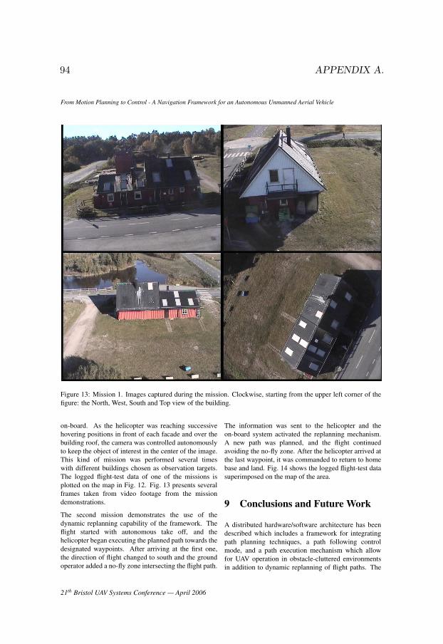
94 APPENDIX A.
From Motion Planning to Control - A Navigation Framework for an Autonomous Unmanned Aerial Vehicle
Figure 13: Mission 1. Images captured during the mission. Clockwise, starting from the upper left corner of thefigure: the North, West, South and Top view of the building.
on-board. As the helicopter was reaching successivehovering positions in front of each facade and over thebuilding roof, the camera was controlled autonomouslyto keep the object of interest in the center of the image.This kind of mission was performed several timeswith different buildings chosen as observation targets.The logged flight-test data of one of the missions isplotted on the map in Fig. 12. Fig. 13 presents severalframes taken from video footage from the missiondemonstrations.
The second mission demonstrates the use of thedynamic replanning capability of the framework. Theflight started with autonomous take off, and thehelicopter began executing the planned path towards thedesignated waypoints. After arriving at the first one,the direction of flight changed to south and the groundoperator added a no-fly zone intersecting the flight path.
The information was sent to the helicopter and theon-board system activated the replanning mechanism.A new path was planned, and the flight continuedavoiding the no-fly zone. After the helicopter arrived atthe last waypoint, it was commanded to return to homebase and land. Fig. 14 shows the logged flight-test datasuperimposed on the map of the area.
9 Conclusions and Future Work
A distributed hardware/software architecture has beendescribed which includes a framework for integratingpath planning techniques, a path following controlmode, and a path execution mechanism which allowfor UAV operation in obstacle-cluttered environmentsin addition to dynamic replanning of flight paths. The
21th Bristol UAV Systems Conference — April 2006
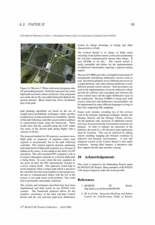
A.2. PAPER II 95
From Motion Planning to Control - A Navigation Framework for an Autonomous Unmanned Aerial Vehicle
Figure 14: Mission 2. White solid arrow designates takeoff and landing position. Solid line represents the actualflight path executed counter-clockwise. Gray polygonalarea marks the no-fly zone added during the flight by theground operator. Black dotted line shows invalidatedpart of the path.
path planning algorithms are based on the use ofsample-based probabilistic techniques which sacrificecompleteness in plan generation for tractability. Detailsof the path following controller are provided in additionto experimental results using the framework. Theseresults show that the controller keeps the UAV withinone meter of the desired path during flights with avelocity of 10 m/s.
The proposed method for 3D trajectory execution viewsflight paths as sequences of segments where eachsegment is incrementally fed to the path followingcontroller. This scheme supports dynamic replanningand replacement of flight path segments (e.g. because ofadding no-fly zones). It also enhances the safety of UAVoperations. The self-contained PFC computer’s role isto request subsequent segments as a mission flight pathis being flown. In cases where the new segments donot arrive on time, the PFC automatically switches toa hover control mode. This approach would help toavoid situations where a longer path which is passed tothe controller becomes unacceptable as time progresses,but due to communication failure with the rest of thesystem, is not made aware of the problem. This couldlead to potentially catastrophic situations.
The systems and techniques described here have beenimplemented and fully tested on our WITAS UAVsystems. The framework proposed allows for theseamless coexistence of the hard real-time ControlKernel and the soft real-time high-level deliberative
system by taking advantage of timing and othercharacteristics of both.
The Control Kernel is in charge of flight modeswitching of the hybrid control system and coordinatingthe real-time communication among other things. Ituses HCSMs to do this. The control kernel iseasily extendible and allows for the implementationof additional functionality requiring a rigorous timingregime.
The use of CORBA provides a straightforward means oftransparently distributing deliberative services such astask- and motion planners across different processors ina single platform, onto other airborne platforms or ontodifferent ground control stations. Task procedures areused in the implementation of reactive behaviors whichprovide the software and conceptual glue between thelower control layer and the upper deliberative layer inthe architecture. Because CORBA is being used, bothreactive behaviors and deliberative functionalities canbe implemented in many different languages as long asthey have supporting IDL mappings.
Future work includes extending two of the servicesused in the dynamic replanning technique, namely, theStrategy Selector and the Strategy Library services.On the hardware side, inclusion of additional sensorsnecessary for perceiving the environment reactively areplanned. In order to enhance the autonomy of theplatform, the need for a 3D elevation map requirementmust be loosened. This can be achieved by addingsensors enabling mapping and obstacle avoidance inunknown and dynamic environments. A new andenhanced version of the Control Kernel is also underevaluation. Among other features, it introduces dataflow support into the state machine concept.
10 Acknowledgements
This work is funded by the Wallenberg Project underthe WITAS UAV Project. Many members of the WITASUAV project helped to make this work possible.
References1. MARVIN: TU Berlin.
http://pdv.cs.tu-berlin.de/MARVIN/.
2. M. La Civita. Integrated Modeling and RobustControl for Full-Envelope Flight of Robotic
21th Bristol UAV Systems Conference — April 2006

96 APPENDIX A.
From Motion Planning to Control - A Navigation Framework for an Autonomous Unmanned Aerial Vehicle
Helicopters. PhD thesis, Carnegie MellonUniversity, Pittsburgh, PA, 2003.
3. G. Conte, S. Duranti, and T. Merz. Dynamic 3DPath Following for an Autonomous Helicopter.In Proc. of the IFAC Symp. on IntelligentAutonomous Vehicles, 2004.
4. P. Doherty, P. Haslum, F. Heintz, T. Merz,T. Persson, and B. Wingman. A DistributedArchitecture for Autonomous Unmanned AerialVehicle Experimentation. In Proc. of theInt. Symp. on Distributed Autonomous RoboticSystems, pages 221–230, 2004.
5. M. Egerstedt, X. Hu, and A. Stotsky. Controlof mobile platforms using a virtual vehicleapproach. IEEE Transactions on AutomaticControl, 46(11):1777–1782, November 2001.
6. E. Frazzoli, M. Dahleh, and E. Feron. RobustHybrid Control for Autonomous VehiclesMotion Planning. In Technical report,Laboratory for Information and DecisionSystems, Massachusetts Institute of Technology,Cambridge, MA, 1999. Technical reportLIDS-P-2468., 1999.
7. S. Gottschalk, M. C. Lin, and D. Manocha.OBBTree: A hierarchical structure for rapidinterference detection. Computer Graphics,30(Annual Conference Series):171–180, 1996.
8. D. Harel. Statecharts: A visual formalismfor complex systems. Science of ComputerProgramming, 8(3):231–274, June 1987.
9. MIT/Draper Autonomous Helicopter Project.http://web.mit.edu/whall/www/heli/.
10. E. N. Johnson and S.K. Kannan. Adaptive flightcontrol for an autonomous unmanned helicopter.In AIAA Guidance, Navigation, and ControlConference and Exhibit, 2002.
11. L. E. Kavraki, P. Svestka, J.C. Latombe, andM. H. Overmars. Probabilistic Roadmapsfor Path Planning in High DimensionalConfiguration Spaces. Proc. of the IEEETransactions on Robotics and Automation,12(4):566–580, 1996.
12. J. J. Kuffner and S. M. LaValle. RRT-connect:An Efficient Approach to Single-Query PathPlanning. In Proc. of the IEEE Int. Conf.on Robotics and Automation, pages 995–1001,2000.
13. P Mantegazza et. al. RTAI: Real time applicationinterface. Linux Journal, 72, April 2000.
14. T. Merz. Building a System for AutonomousAerial Robotics Research. In Proc. of the IFACSymp. on Intelligent Autonomous Vehicles, 2004.
15. T. Merz, S. Duranti, and G. Conte. Autonomouslanding of an unmanned aerial helicopter basedon vision and inertial sensing. In Proc. of the9th International Symposium on ExperimentalRobotics, 2004.
16. B. Mettler, M.B. Tischler, and T. Kanade.System identification modeling of a small-scaleunmanned helicopter. Journal of the AmericanHelicopter Society, October 2001.
17. P-O Pettersson. Using Randomized Algorithmsfor Helicopter Path Planning. Lic. ThesisLinkoping University., 2006.
18. P-O Pettersson and P. Doherty. ProbabilisticRoadmap Based Path Planning for anAutonomous Unmanned Aerial Vehicle. InProc. of the ICAPS-04 Workshop on ConnectingPlanning Theory with Practice, 2004.
19. AVATAR: USC Autonomous Flying VehicleProject. http://www-robotics.usc.edu/∼avatar.
20. BEAR: Berkeley Aerorobot Team.http://robotics.eecs.berkeley.edu/bear/.
21. Georgia Tech UAV.http://www.ae.gatech.edu/labs/controls/uavrf/.
22. Hummingbird: Stanford University.http://sun-valley.stanford.edu/users/heli/.
23. CMU Autonomous Helicopter Project.www.cs.cmu.edu/afs/cs/project/chopper/www.
24. M. Wzorek and P. Doherty. PreliminaryReport: Reconfigurable Path Planning for anAutonomous Unmanned Aerial Vehicle. InProceedings of the 24th Annual Workshop of theUK Planning and Scheduling Special InterestGroup (PlanSIG-05), 2005.
21th Bristol UAV Systems Conference — April 2006
A.3. PAPER III 97
A.3 Paper III
Autonomous Landing of an UnmannedHelicopter based on Vision and InertialSensing
Torsten Merz, Simone Duranti, and Gianpaolo Conte
Department of Computer and Information ScienceLinkoping University, SE-58183 Linkoping, Sweden
Abstract. In this paper, we propose an autonomous precision landing method foran unmanned helicopter based on an on-board visual navigation system consistingof a single pan-tilting camera, off-the-shelf computer hardware and inertial sensors.Compared to existing methods, the system doesn’t depend on additional sensors (inparticular not on GPS), offers a wide envelope of starting points for the autonomousapproach, and is robust to different weather conditions. Helicopter position andattitude is estimated from images of a specially designed landing pad. We provideresults from both simulations and flight tests, showing the performance of the visionsystem and the overall quality of the landing.
1 Introduction
Many autonomous landing systems for Unmanned Aerial Vehicles (UAVs)are based on GPS and a dedicated close range sensor for accurate altitudemeasurement (radar altimeter, sonar, infrared or theodolites). However, inurban environments buildings and other obstacles disturb the GPS signaland can even cause loss of signal (multi-path effects, EM noise due to ac-tive emitters). Once the GPS signal is lost, the dead reckoning capability ofaffordable on-board inertial navigation systems does not allow precision navi-gation for more than few seconds, before diverging. Hence the need of a robustobservation of the position: a vision system is self-contained, not jammable,and provides in the proposed implementation a position measurement oneorder of magnitude more accurate than standard GPS (cm accuracy or bet-ter). Estimating velocity from vision is difficult due to limited image framerate and sensor resolution. In the proposed method velocity is estimated ac-curately and robustly by fusing vision position with the measurements ofinertial sensors that usually belong to the standard instrumentation of anUAV for stabilization. The problem is to develop: (a) a vision system with asufficient operating range to allow robust pose estimation from a reasonabledistance at a sufficient rate with low latency using a landing pad of mini-mal size; (b) a method to fuse these data with inertial measurements; (c) asuitable flight controller. In an autonomous landing system all componentshave to match each other. For instance, for calculating vision estimates a

98 APPENDIX A.
Fig. 1. The WITAS helicopter descend-ing to the landing pad.
Fig. 2. Landing pad with reference pat-tern seen from the on-board camera.
proper trade-off between accuracy, range, latency, and rate has to be foundoptimizing the overall performance of the system.
Our method requires a special landing pad (Fig. 2). As unmanned heli-copters usually operate from a designated home base this is not a real con-straint. A precise and fast pan/tilt camera is used to extend the range ofthe vision system and decouple the helicopter attitude from the vision field.We developed a single camera solution, as multi-camera systems make thesystem more complex and expensive and don’t offer significant advantageswhen using known landmarks. For the experimentation we used a helicopterplatform (Fig. 1) which had been developed in the WITAS project [2,1].
Vision-based control of small size autonomous helicopters is an activearea of research. A good overview of the state-of-the-art can be found in[7]. Our contribution to the landing problem consists of: (a) many demon-strated landings with a system only based on images from a single cameraand inertial data using off-the-shelf computer hardware; (b) a wide envelopeof starting points for the autonomous approach; (c) robustness to differentweather conditions (wind, ambient light); (d) a quantitative evaluation of thevision system and the landing performance.
2 Vision System
The vision system consists of a camera mounted on a pan/tilt unit (PTU),a computer for image processing, and a landing pad (a foldable plate) witha reference pattern on its surface. In this section, we explain the design ofthe reference pattern, describe the image formation, and present the imageprocessing algorithm.
The reference pattern is designed to fulfill the following criteria: fast recog-nition, accurate pose estimation for close and distant range, minimum size,and minimal asymmetry. We have chosen black circles on white backgroundas they are fast to detect and provide accurate image features (Fig. 2). From

A.3. PAPER III 99
the projection of three circles lying on the corner points of an equilateraltriangle the pose of an object is uniquely determined, assuming all intrin-sic camera parameters are known. Circles are projected as ellipses, describedby the center point ue, the semi-major axis la, the semi-minor axis lb, andthe semi-major axis angle θe The pose of the landing pad with respect tothe camera coordinate system is estimated by minimizing the reprojectionerror of the extracted center points and semi-axes of the three ellipses. Weuse five circle triplets of different size (radius 2 to 32 cm, distance 8 to 128cm) with common center point to achieve a wide range of possible camerapositions. Each triplet is uniquely determined by a combination of differentlysized inner circles.
A point px in the landing pad frame is projected on the image plane asfollows:
u = P px =
αu 0 u0 00 αv v0 00 0 1 0
(cpR
ctp0T
3 1
)px u ∈ P2 px ∈ P3 (1)
The extrinsic camera parameters are given by the three Euler angles of therotation matrix c
pR and the three components of the translation vector ctp. Weuse a camera model with the following intrinsic parameters: ”focal lengths”αu and αv in pixels, principal point (u0, v0), and four lens distortion coef-ficients . All intrinsic parameters are calibrated using Bouguet’s calibrationtoolbox [3]. A conic in P2 is the locus of all points u satisfying the homoge-neous quadratic equation uTC u = 0. The transformation of a circle Cp onthe landing pad into an ellipse Ci in the image plane is given by[4]:
Ci = (H−1)TCpH−1 (2)
The homography matrix H is the projection matrix P without third column(z = 0). We calculate the ellipse center and axes from Ci and represent theparameters in a common feature vector c.
Fig. 3 shows a data flow diagram of the vision system. Round-edged boxesrepresent image processing functions, sharp-edged boxes indicate independentprocesses, and dashed lines show trigger connections. Closed contours areextracted from gray-level images using a fast contour following algorithmwith two parameters: edge strength and binarization threshold. The latteris calculated from the intensity distribution of the reference pattern. In thecontour list we search for the three biggest ellipses belonging to a circletriplet. Ellipse parameters are estimated by minimizing the algebraic distanceof undistorted contour points to the conic using SVD [4,6]. After havingfound three ellipses, the corresponding contours are resampled with sub-pixelaccuracy. A coarse pose is estimated based on the ratio of semi-major axes
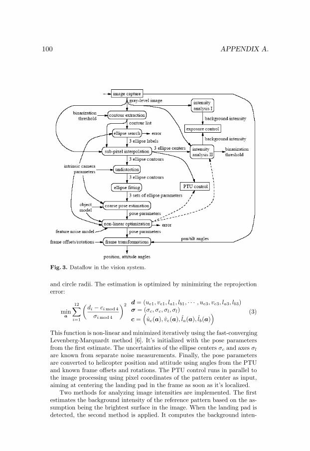
100 APPENDIX A.
Fig. 3. Dataflow in the vision system.
and circle radii. The estimation is optimized by minimizing the reprojectionerror:
mina
12∑i=1
(di − ci mod 4
σi mod 4
)2 d = (ue1, ve1, la1, lb1, · · · , ue3, ve3, la3, lb3)σ = (σc, σc, σl, σl)c =
(ue(a), ve(a), la(a), lb(a)
) (3)
This function is non-linear and minimized iteratively using the fast-convergingLevenberg-Marquardt method [6]. It’s initialized with the pose parametersfrom the first estimate. The uncertainties of the ellipse centers σc and axes σl
are known from separate noise measurements. Finally, the pose parametersare converted to helicopter position and attitude using angles from the PTUand known frame offsets and rotations. The PTU control runs in parallel tothe image processing using pixel coordinates of the pattern center as input,aiming at centering the landing pad in the frame as soon as it’s localized.
Two methods for analyzing image intensities are implemented. The firstestimates the background intensity of the reference pattern based on the as-sumption being the brightest surface in the image. When the landing pad isdetected, the second method is applied. It computes the background inten-

A.3. PAPER III 101
newcameraupdate
Tbo > Tlim1∆ P< ∆ max
KFprediction
INSmechanization
Tbo
filter
initialization
updateKF
Tbo=0
Tbo > Tlim2
no
yesno
yesyes
no
yes
no
Fig. 4. The filter architecture.
sity and the binarization threshold based on the intensity distribution of thepattern. The exposure controller controls the camera shutter time and irisaiming at keeping the background intensity in a certain range.
3 Sensor Fusion
The position and attitude estimates provided by the vision system can notbe fed directly into the controller due to their intrinsic lack of robustness:the field of view can be temporarily occluded (for example by the landinggear), the illumination conditions can change dramatically just by movingfew meters (sun reflections, shades, etc.). On the other hand, vision readingsare very accurate, when available.
Hence, a navigation filter based on a Kalman filter (KF) has been devel-oped, fusing highly accurate 3D position estimates from the vision systemwith inertial data provided by the on-board accelerometers and angular rategyros. Besides filtering out a large part of the noise and outliers, the filtersprovides a satisfying dead reckoning capability, sufficient to complete thelanding even when the vision system is ”blind”1, see Fig. 8.
The implementation of the KF is done using the error state space orindirect formulation with feedback mechanization (Fig. 4). The states ofthe filter are the estimated inertial navigation system (INS) errors. The threeobservations are given by the difference between the INS position and theposition from the vision system (lateral, longitudinal and vertical positionrelative to the pattern). The advantage of the indirect formulation versusthe direct formulation (position, velocity and attitude are among the state
1 During the last 50 cm before touch down the vision system is often ”blind” dueto two factors: (a) the shade of the helicopter covers part of the pattern at touchdown, and (b) when the distance of the camera to the pattern is very small it isvery hard for the controller of the pan/tilt unit to keep the pattern in the picture.
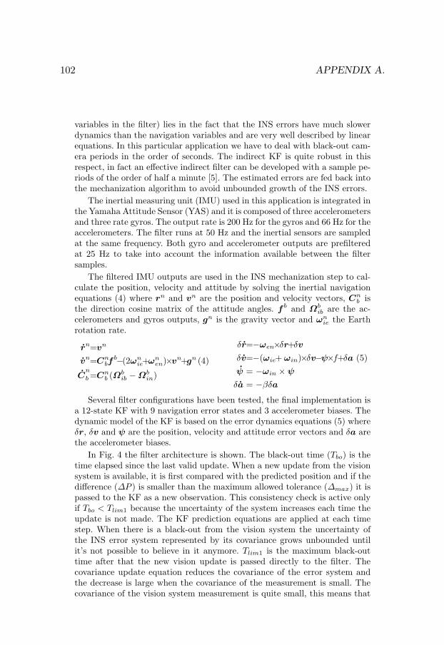
102 APPENDIX A.
variables in the filter) lies in the fact that the INS errors have much slowerdynamics than the navigation variables and are very well described by linearequations. In this particular application we have to deal with black-out cam-era periods in the order of seconds. The indirect KF is quite robust in thisrespect, in fact an effective indirect filter can be developed with a sample pe-riods of the order of half a minute [5]. The estimated errors are fed back intothe mechanization algorithm to avoid unbounded growth of the INS errors.
The inertial measuring unit (IMU) used in this application is integrated inthe Yamaha Attitude Sensor (YAS) and it is composed of three accelerometersand three rate gyros. The output rate is 200 Hz for the gyros and 66 Hz for theaccelerometers. The filter runs at 50 Hz and the inertial sensors are sampledat the same frequency. Both gyro and accelerometer outputs are prefilteredat 25 Hz to take into account the information available between the filtersamples.
The filtered IMU outputs are used in the INS mechanization step to cal-culate the position, velocity and attitude by solving the inertial navigationequations (4) where rn and vn are the position and velocity vectors, Cn
b isthe direction cosine matrix of the attitude angles. f b and Ωb
ib are the ac-celerometers and gyros outputs, gn is the gravity vector and ωn
ie the Earthrotation rate.
rn=vn
vn=Cnbf
b−(2ωnie+ω
nen)×vn+gn (4)
Cn
b =Cnb (Ωb
ib −Ωbin)
δr=−ωen×δr+δvδv=−(ωie+ ωin)×δv−ψ×f+δa (5)ψ = −ωin ×ψδa = −βδa
Several filter configurations have been tested, the final implementation isa 12-state KF with 9 navigation error states and 3 accelerometer biases. Thedynamic model of the KF is based on the error dynamics equations (5) whereδr, δv and ψ are the position, velocity and attitude error vectors and δa arethe accelerometer biases.
In Fig. 4 the filter architecture is shown. The black-out time (Tbo) is thetime elapsed since the last valid update. When a new update from the visionsystem is available, it is first compared with the predicted position and if thedifference (∆P ) is smaller than the maximum allowed tolerance (∆max) it ispassed to the KF as a new observation. This consistency check is active onlyif Tbo < Tlim1 because the uncertainty of the system increases each time theupdate is not made. The KF prediction equations are applied at each timestep. When there is a black-out from the vision system the uncertainty ofthe INS error system represented by its covariance grows unbounded untilit’s not possible to believe in it anymore. Tlim1 is the maximum black-outtime after that the new vision update is passed directly to the filter. Thecovariance update equation reduces the covariance of the error system andthe decrease is large when the covariance of the measurement is small. Thecovariance of the vision system measurement is quite small, this means that
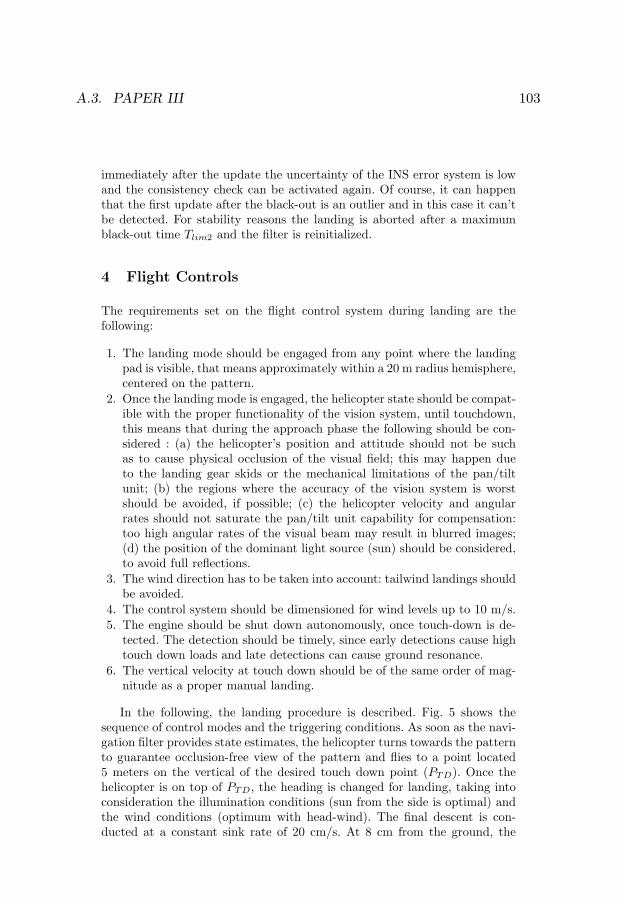
A.3. PAPER III 103
immediately after the update the uncertainty of the INS error system is lowand the consistency check can be activated again. Of course, it can happenthat the first update after the black-out is an outlier and in this case it can’tbe detected. For stability reasons the landing is aborted after a maximumblack-out time Tlim2 and the filter is reinitialized.
4 Flight Controls
The requirements set on the flight control system during landing are thefollowing:
1. The landing mode should be engaged from any point where the landingpad is visible, that means approximately within a 20 m radius hemisphere,centered on the pattern.
2. Once the landing mode is engaged, the helicopter state should be compat-ible with the proper functionality of the vision system, until touchdown,this means that during the approach phase the following should be con-sidered : (a) the helicopter’s position and attitude should not be suchas to cause physical occlusion of the visual field; this may happen dueto the landing gear skids or the mechanical limitations of the pan/tiltunit; (b) the regions where the accuracy of the vision system is worstshould be avoided, if possible; (c) the helicopter velocity and angularrates should not saturate the pan/tilt unit capability for compensation:too high angular rates of the visual beam may result in blurred images;(d) the position of the dominant light source (sun) should be considered,to avoid full reflections.
3. The wind direction has to be taken into account: tailwind landings shouldbe avoided.
4. The control system should be dimensioned for wind levels up to 10 m/s.5. The engine should be shut down autonomously, once touch-down is de-
tected. The detection should be timely, since early detections cause hightouch down loads and late detections can cause ground resonance.
6. The vertical velocity at touch down should be of the same order of mag-nitude as a proper manual landing.
In the following, the landing procedure is described. Fig. 5 shows thesequence of control modes and the triggering conditions. As soon as the navi-gation filter provides state estimates, the helicopter turns towards the patternto guarantee occlusion-free view of the pattern and flies to a point located5 meters on the vertical of the desired touch down point (PTD). Once thehelicopter is on top of PTD, the heading is changed for landing, taking intoconsideration the illumination conditions (sun from the side is optimal) andthe wind conditions (optimum with head-wind). The final descent is con-ducted at a constant sink rate of 20 cm/s. At 8 cm from the ground, the

104 APPENDIX A.
Fig. 5. Mode sequence leading to touch down. Note that all transitions are one-directional: once a mode is exited it can not be re-entered.
throttle command is ramped down, inducing loss of lift and touch down.
The control laws of the helicopter consist of an inner loop (pitch, roll andyaw angle control, and vertical velocity control) and an outer loop (positionand velocity control). The inner loop consists of the Yamaha Attitude ControlSystem (YACS), the properties of which have been identified with a dedicatedsystem identification session. The control equations of the outer loop can besummarized as following:
θC = KpxδX +KpvxδVX +KivxδVXsum
∆φC = KpyδY +KpvyδVY +KivyδVY sum
VZC = KivzδVZsum +Kpvz(VZtarget − VZ) (6)VZtarget = limit(0.75δZ, VZmin, VZmax)
ωC = limit(Kpwδψ,−26 deg/s, 26 deg/s)
where the subscripted K are control gains, the δ are control errors, thesubscript sum indicates the integral terms, θC is the commanded pitch angle,∆φC is the commanded roll angle variation, ωC is the commanded yaw rateand VZC is the commanded vertical velocity2.
5 Experimental Results
The helicopter used for experimentation is a slightly modified Yamaha RMAX(Fig. 1). It has a total length of 3.6 m (incl. main rotor) and a take-off weight2 During the descent and touch down phases, the gains of the velocity terms (Kpvx
and Kpvx) are increased by one fifth and the integral terms in the horizontalcontrol are activated, for faster and more precise position control.

A.3. PAPER III 105
0 2 4 6 8 10 12 14 16 18 200
2
4
6
8
10
12
14
16
18
20
distance to pattern [m]
altit
ude
[m]
[mm]
50
100
150
200
250
300
350
400
0 2 4 6 8 10 12 14 16 18 200
2
4
6
8
10
12
14
16
18
20
distance to pattern [m]
altit
ude
[m]
[mm]
5
10
15
20
25
30
Fig. 6. RMS error in horizontal (left) and vertical position (right) from simulation.
of 95 kg, including 30 kg available for payload. The vision navigation systemconsists of two PC104 stacks with PIII 700 MHz processors, the inertialsensors of the YAS, and a single standard CCD camera with approx. 45degrees horizontal angle of view which is mounted on an off-the-shelf pan/tiltunit (PTU). One of the two computers is dedicated to sensor managementand low level control of the helicopter, the other one for image processing andcontrol of the camera and the PTU. The two computers communicate over aRS232C serial link. They are built inside a shock and vibration isolated box,which also includes a precision GPS, a barometric altitude sensor, a compass,a video recorder, a video transmitter, and a wireless Ethernet bridge. ThePTU is mechanically limited to 111 degrees tilt and ±180 degrees pan, themax. angular rate is 300 degrees/s and the resolution 0.051 degrees. It ismounted on a vibration isolating platform on the underside of the helicopterbody.
We estimated the RMS error of the vision system in position and atti-tude depending on the relative position to the pattern in leveled flight. Foreach position 1000 samples were generated using a feature noise model thatincluded noise from image formation, digitization, and segmentation. We de-veloped a method to analyze noise in ellipse center position and semi-axislength. Errors introduced by the transformation from the camera frame intothe body frame were not considered in simulation. Fig. 6 shows the RMS er-rors (1σ) in horizontal and vertical position. The error doesn’t change muchin the simulated envelope (a 20 m radius hemisphere, with a ”blind” sectorfrom azimuth 0 to 15 degrees) due to different triplet sizes and sub-pixelfeature extraction. For pitch and roll the error behaves similar to the hori-zontal error, with a maximum RMS value of ≈1 degree, the error in headingis negligible.
The actual accuracy of the vision system was evaluated through an in-flight comparison with a navigation solution based on the YAS and a precisionRTK GPS which supplied horizontal/vertical position with 10 mm/15 mm

106 APPENDIX A.
Fig. 7. Position and heading estimatesfrom the vision system vs. estimatesbased on YAS and precision RTK GPSobservations.
418 419 420 421 422 423 424 4250
0.2
0.4
0.6
0.8
1
altit
ude
[m]
time [s]
filterraw vision altitude
pattern occluded bythe shade of the helicopter
last valid vision measurement
touch down
Fig. 8. Altitude estimates from the nav-igation filter when losing vision.
Fig. 9. Time histories and control modesduring autonomous landing. The dashedlines show readings from a standardINS/DGPS unit.
uncertainty (1σ). We found good agreement between measured and simulatederrors. Fig. 7 shows timeplots for distance, altitude, and pitch angle at typicalstarting points for autonomous landing. Position and attitude estimates wereprovided with an average rate of 20 Hz (using 384×288 pixels images) andan average latency of 110 ms (including delays from capturing PAL signals).
Some tens of autonomous landings were conducted from different rela-tive positions to the landing pad within the specified envelope, on grass andsnow fields, with different wind and illumination conditions. A sample of theresults is available in Fig. 10 . The vertical velocity at touch down rangedbetween 18 and 35 cm/s, this corresponds to load factors of about 1.4 g ongrass fields. The horizontal velocity at touch down was in the order of mag-nitude of 15 cm/s. The average touch down point precision was about 42cm (13 % of rotor diameter). Thanks to the pan/tilt camera and a robustcontroller, considerable wind levels can be handled. Successful landings havebeen performed with wind levels on ground up to 30 km/h (2 min average),with gusts of 45 km/h.

A.3. PAPER III 107
Fig. 10. Flight test results from several autonomous landings.
6 Acknowledgements
We thank Piotr Rudol and Mariusz Wzorek for providing the pan-tilt con-troller and Anke Knoppler for work on camera calibration. This work wassupported by the Wallenberg Foundation, Sweden.
References
1. P. Doherty. Advanced research with autonomous unmanned aerial vehicles. InProc. of the 9th International Conference on the Principles of Knowledge Rep-resentation and Reasoning, pages 731–732, June 2004.
2. P. Doherty, P. Haslum, F. Heintz, T. Merz, T. Persson, and B. Wingman. Adistributed architecture for autonomous unmanned aerial vehicle experimenta-tion. In Proc. of the 7th International Symposium on Distributed AutonomousRobotic Systems, pages 221–230, June 2004.
3. Jean-Yves Bouguet. Camera Calibration Toolbox for Matlab .http://www.vision.caltech.edu/bouguetj/calib doc.
4. K. Kanatani. Geometric Computation for Machine Vision. Oxford UniversityPress, 1995.
5. P.S. Maybeck. Stochastic models, estimation, and control. In Mathematics inScience and Engineering, volume 141-1, pages 289–367. Academic Press, 1979.
6. W.H. Press, S.A. Teukolsky, W.T. Vetterling, and B.P. Flannery. NumericalRecipes in C: The Art of Scientific Computing. Cambridge University Press,1992.
7. S. Saripalli, J.F. Montgomery, and G. Sukhatme. Visually-guided landing ofan unmanned aerial vehicle. IEEE Transactions on Robotics and Automation,19(3):371–380, June 2003.


LINKÖPINGS UNIVERSITET
Rapporttyp Report category
Licentiatavhandling
Examensarbete
C-uppsats
D-uppsats
Övrig rapport
Språk Language
Svenska/Swedish
Engelska/English
Titel Title
Författare Author
Sammanfattning Abstract
ISBN
ISRN
Serietitel och serienummer ISSN Title of series, numbering
Linköping Studies in Science and Technology
Thesis No. 1307
Nyckelord Keywords
Datum Date
URL för elektronisk version
X
X
March 1st, 2007
Avdelning, institution Division, department
Institutionen för datavetenskap
Department of Computer and Information Science
Navigation Functionalities for an Autonomous UAV Helicopter
Gianpaolo Conte
This thesis was written during the WITAS UAV Project where one of the goals has been the development of a software/hardware architecture for an unmanned autonomous helicopter, in addition to autonomous functionalities required for complex mission scenarios. The algorithms developed here have been tested on an unmanned helicopter platform developed by Yamaha Motor Company called the RMAX. The character of the thesis is primarily experimental and it should be viewed as developing navigational functionality to support autonomous flight during complex real-world mission scenarios. This task is multidisciplinary since it requires competence in aeronautics, computer science and electronics. The focus of the thesis has been on the development of a control method to enable the helicopter to follow 3D paths. Additionally, a helicopter simulation tool has been developed in order to test the control system before flight-tests. The thesis also presents an implementation and experimental evaluation of a sensor fusion technique based on a Kalman filter applied to a vision based autonomous landing problem. Extensive experimental flight-test results are presented.
Unmanned Aerial Vehicle, Control System, Path Following, Path Planning, Sensor Fusion, Vision Based Landing, Kalman Filter, Real-Time.
978-91-85715-35-0
0280-7971
LiU-Tek-Lic-2007:16


Department of Computer and Information ScienceLinköpings universitet
Linköping Studies in Science and TechnologyFaculty of Arts and Sciences - Licentiate Theses
No 17 Vojin Plavsic: Interleaved Processing of Non-Numerical Data Stored on a Cyclic Memory. (Available at:FOA, Box 1165, S-581 11 Linköping, Sweden. FOA Report B30062E)
No 28 Arne Jönsson, Mikael Patel: An Interactive Flowcharting Technique for Communicating and Realizing Al-gorithms, 1984.
No 29 Johnny Eckerland: Retargeting of an Incremental Code Generator, 1984.No 48 Henrik Nordin: On the Use of Typical Cases for Knowledge-Based Consultation and Teaching, 1985.No 52 Zebo Peng: Steps Towards the Formalization of Designing VLSI Systems, 1985.No 60 Johan Fagerström: Simulation and Evaluation of Architecture based on Asynchronous Processes, 1985.No 71 Jalal Maleki: ICONStraint, A Dependency Directed Constraint Maintenance System, 1987.No 72 Tony Larsson: On the Specification and Verification of VLSI Systems, 1986.No 73 Ola Strömfors: A Structure Editor for Documents and Programs, 1986.No 74 Christos Levcopoulos: New Results about the Approximation Behavior of the Greedy Triangulation, 1986.No 104 Shamsul I. Chowdhury: Statistical Expert Systems - a Special Application Area for Knowledge-Based Com-
puter Methodology, 1987.No 108 Rober Bilos: Incremental Scanning and Token-Based Editing, 1987.No 111 Hans Block: SPORT-SORT Sorting Algorithms and Sport Tournaments, 1987.No 113 Ralph Rönnquist: Network and Lattice Based Approaches to the Representation of Knowledge, 1987.No 118 Mariam Kamkar, Nahid Shahmehri: Affect-Chaining in Program Flow Analysis Applied to Queries of Pro-
grams, 1987.No 126 Dan Strömberg: Transfer and Distribution of Application Programs, 1987.No 127 Kristian Sandahl: Case Studies in Knowledge Acquisition, Migration and User Acceptance of Expert Sys-
tems, 1987. No 139 Christer Bäckström: Reasoning about Interdependent Actions, 1988.No 140 Mats Wirén: On Control Strategies and Incrementality in Unification-Based Chart Parsing, 1988.No 146 Johan Hultman: A Software System for Defining and Controlling Actions in a Mechanical System, 1988.No 150 Tim Hansen: Diagnosing Faults using Knowledge about Malfunctioning Behavior, 1988.No 165 Jonas Löwgren: Supporting Design and Management of Expert System User Interfaces, 1989.No 166 Ola Petersson: On Adaptive Sorting in Sequential and Parallel Models, 1989.No 174 Yngve Larsson: Dynamic Configuration in a Distributed Environment, 1989.No 177 Peter Åberg: Design of a Multiple View Presentation and Interaction Manager, 1989.No 181 Henrik Eriksson: A Study in Domain-Oriented Tool Support for Knowledge Acquisition, 1989.No 184 Ivan Rankin: The Deep Generation of Text in Expert Critiquing Systems, 1989.No 187 Simin Nadjm-Tehrani: Contributions to the Declarative Approach to Debugging Prolog Programs, 1989.No 189 Magnus Merkel: Temporal Information in Natural Language, 1989.No 196 Ulf Nilsson: A Systematic Approach to Abstract Interpretation of Logic Programs, 1989.No 197 Staffan Bonnier: Horn Clause Logic with External Procedures: Towards a Theoretical Framework, 1989.No 203 Christer Hansson: A Prototype System for Logical Reasoning about Time and Action, 1990.No 212 Björn Fjellborg: An Approach to Extraction of Pipeline Structures for VLSI High-Level Synthesis, 1990.No 230 Patrick Doherty: A Three-Valued Approach to Non-Monotonic Reasoning, 1990.No 237 Tomas Sokolnicki: Coaching Partial Plans: An Approach to Knowledge-Based Tutoring, 1990.No 250 Lars Strömberg: Postmortem Debugging of Distributed Systems, 1990.No 253 Torbjörn Näslund: SLDFA-Resolution - Computing Answers for Negative Queries, 1990.No 260 Peter D. Holmes: Using Connectivity Graphs to Support Map-Related Reasoning, 1991.No 283 Olof Johansson: Improving Implementation of Graphical User Interfaces for Object-Oriented Knowledge-
Bases, 1991.No 298 Rolf G Larsson: Aktivitetsbaserad kalkylering i ett nytt ekonomisystem, 1991.No 318 Lena Srömbäck: Studies in Extended Unification-Based Formalism for Linguistic Description: An Algorithm
for Feature Structures with Disjunction and a Proposal for Flexible Systems, 1992.No 319 Mikael Pettersson: DML-A Language and System for the Generation of Efficient Compilers from Denotatio-
nal Specification, 1992.No 326 Andreas Kågedal: Logic Programming with External Procedures: an Implementation, 1992.No 328 Patrick Lambrix: Aspects of Version Management of Composite Objects, 1992.No 333 Xinli Gu: Testability Analysis and Improvement in High-Level Synthesis Systems, 1992.No 335 Torbjörn Näslund: On the Role of Evaluations in Iterative Development of Managerial Support Sytems,
1992.No 348 Ulf Cederling: Industrial Software Development - a Case Study, 1992.No 352 Magnus Morin: Predictable Cyclic Computations in Autonomous Systems: A Computational Model and Im-
plementation, 1992.No 371 Mehran Noghabai: Evaluation of Strategic Investments in Information Technology, 1993.No 378 Mats Larsson: A Transformational Approach to Formal Digital System Design, 1993.No 380 Johan Ringström: Compiler Generation for Parallel Languages from Denotational Specifications, 1993.No 381 Michael Jansson: Propagation of Change in an Intelligent Information System, 1993.No 383 Jonni Harrius: An Architecture and a Knowledge Representation Model for Expert Critiquing Systems, 1993.No 386 Per Österling: Symbolic Modelling of the Dynamic Environments of Autonomous Agents, 1993.No 398 Johan Boye: Dependency-based Groudness Analysis of Functional Logic Programs, 1993.

No 402 Lars Degerstedt: Tabulated Resolution for Well Founded Semantics, 1993.No 406 Anna Moberg: Satellitkontor - en studie av kommunikationsmönster vid arbete på distans, 1993.No 414 Peter Carlsson: Separation av företagsledning och finansiering - fallstudier av företagsledarutköp ur ett agent-
teoretiskt perspektiv, 1994.No 417 Camilla Sjöström: Revision och lagreglering - ett historiskt perspektiv, 1994.No 436 Cecilia Sjöberg: Voices in Design: Argumentation in Participatory Development, 1994.No 437 Lars Viklund: Contributions to a High-level Programming Environment for a Scientific Computing, 1994.No 440 Peter Loborg: Error Recovery Support in Manufacturing Control Systems, 1994.FHS 3/94 Owen Eriksson: Informationssystem med verksamhetskvalitet - utvärdering baserat på ett verksamhetsinrik-
tat och samskapande perspektiv, 1994.FHS 4/94 Karin Pettersson: Informationssystemstrukturering, ansvarsfördelning och användarinflytande - En kompa-
rativ studie med utgångspunkt i två informationssystemstrategier, 1994.No 441 Lars Poignant: Informationsteknologi och företagsetablering - Effekter på produktivitet och region, 1994.No 446 Gustav Fahl: Object Views of Relational Data in Multidatabase Systems, 1994.No 450 Henrik Nilsson: A Declarative Approach to Debugging for Lazy Functional Languages, 1994.No 451 Jonas Lind: Creditor - Firm Relations: an Interdisciplinary Analysis, 1994.No 452 Martin Sköld: Active Rules based on Object Relational Queries - Efficient Change Monitoring Techniques,
1994.No 455 Pär Carlshamre: A Collaborative Approach to Usability Engineering: Technical Communicators and System
Developers in Usability-Oriented Systems Development, 1994.FHS 5/94 Stefan Cronholm: Varför CASE-verktyg i systemutveckling? - En motiv- och konsekvensstudie avseende ar-
betssätt och arbetsformer, 1994.No 462 Mikael Lindvall: A Study of Traceability in Object-Oriented Systems Development, 1994.No 463 Fredrik Nilsson: Strategi och ekonomisk styrning - En studie av Sandviks förvärv av Bahco Verktyg, 1994.No 464 Hans Olsén: Collage Induction: Proving Properties of Logic Programs by Program Synthesis, 1994.No 469 Lars Karlsson: Specification and Synthesis of Plans Using the Features and Fluents Framework, 1995.No 473 Ulf Söderman: On Conceptual Modelling of Mode Switching Systems, 1995.No 475 Choong-ho Yi: Reasoning about Concurrent Actions in the Trajectory Semantics, 1995.No 476 Bo Lagerström: Successiv resultatavräkning av pågående arbeten. - Fallstudier i tre byggföretag, 1995.No 478 Peter Jonsson: Complexity of State-Variable Planning under Structural Restrictions, 1995.FHS 7/95 Anders Avdic: Arbetsintegrerad systemutveckling med kalkylkprogram, 1995.No 482 Eva L Ragnemalm: Towards Student Modelling through Collaborative Dialogue with a Learning Compani-
on, 1995.No 488 Eva Toller: Contributions to Parallel Multiparadigm Languages: Combining Object-Oriented and Rule-Based
Programming, 1995.No 489 Erik Stoy: A Petri Net Based Unified Representation for Hardware/Software Co-Design, 1995.No 497 Johan Herber: Environment Support for Building Structured Mathematical Models, 1995.No 498 Stefan Svenberg: Structure-Driven Derivation of Inter-Lingual Functor-Argument Trees for Multi-Lingual
Generation, 1995.No 503 Hee-Cheol Kim: Prediction and Postdiction under Uncertainty, 1995.FHS 8/95 Dan Fristedt: Metoder i användning - mot förbättring av systemutveckling genom situationell metodkunskap
och metodanalys, 1995.FHS 9/95 Malin Bergvall: Systemförvaltning i praktiken - en kvalitativ studie avseende centrala begrepp, aktiviteter och
ansvarsroller, 1995.No 513 Joachim Karlsson: Towards a Strategy for Software Requirements Selection, 1995.No 517 Jakob Axelsson: Schedulability-Driven Partitioning of Heterogeneous Real-Time Systems, 1995.No 518 Göran Forslund: Toward Cooperative Advice-Giving Systems: The Expert Systems Experience, 1995.No 522 Jörgen Andersson: Bilder av småföretagares ekonomistyrning, 1995.No 538 Staffan Flodin: Efficient Management of Object-Oriented Queries with Late Binding, 1996.No 545 Vadim Engelson: An Approach to Automatic Construction of Graphical User Interfaces for Applications in
Scientific Computing, 1996.No 546 Magnus Werner : Multidatabase Integration using Polymorphic Queries and Views, 1996.FiF-a 1/96 Mikael Lind: Affärsprocessinriktad förändringsanalys - utveckling och tillämpning av synsätt och metod,
1996.No 549 Jonas Hallberg: High-Level Synthesis under Local Timing Constraints, 1996.No 550 Kristina Larsen: Förutsättningar och begränsningar för arbete på distans - erfarenheter från fyra svenska fö-
retag. 1996.No 557 Mikael Johansson: Quality Functions for Requirements Engineering Methods, 1996.No 558 Patrik Nordling: The Simulation of Rolling Bearing Dynamics on Parallel Computers, 1996.No 561 Anders Ekman: Exploration of Polygonal Environments, 1996.No 563 Niclas Andersson: Compilation of Mathematical Models to Parallel Code, 1996.No 567 Johan Jenvald: Simulation and Data Collection in Battle Training, 1996.No 575 Niclas Ohlsson: Software Quality Engineering by Early Identification of Fault-Prone Modules, 1996.No 576 Mikael Ericsson: Commenting Systems as Design Support—A Wizard-of-Oz Study, 1996.No 587 Jörgen Lindström: Chefers användning av kommunikationsteknik, 1996.No 589 Esa Falkenroth: Data Management in Control Applications - A Proposal Based on Active Database Systems,
1996.No 591 Niclas Wahllöf: A Default Extension to Description Logics and its Applications, 1996.No 595 Annika Larsson: Ekonomisk Styrning och Organisatorisk Passion - ett interaktivt perspektiv, 1997.No 597 Ling Lin: A Value-based Indexing Technique for Time Sequences, 1997.

No 598 Rego Granlund: C3Fire - A Microworld Supporting Emergency Management Training, 1997.No 599 Peter Ingels: A Robust Text Processing Technique Applied to Lexical Error Recovery, 1997.No 607 Per-Arne Persson: Toward a Grounded Theory for Support of Command and Control in Military Coalitions,
1997.No 609 Jonas S Karlsson: A Scalable Data Structure for a Parallel Data Server, 1997.FiF-a 4 Carita Åbom: Videomötesteknik i olika affärssituationer - möjligheter och hinder, 1997.FiF-a 6 Tommy Wedlund: Att skapa en företagsanpassad systemutvecklingsmodell - genom rekonstruktion, värde-
ring och vidareutveckling i T50-bolag inom ABB, 1997.No 615 Silvia Coradeschi: A Decision-Mechanism for Reactive and Coordinated Agents, 1997.No 623 Jan Ollinen: Det flexibla kontorets utveckling på Digital - Ett stöd för multiflex? 1997.No 626 David Byers: Towards Estimating Software Testability Using Static Analysis, 1997.No 627 Fredrik Eklund: Declarative Error Diagnosis of GAPLog Programs, 1997.No 629 Gunilla Ivefors: Krigsspel coh Informationsteknik inför en oförutsägbar framtid, 1997.No 631 Jens-Olof Lindh: Analysing Traffic Safety from a Case-Based Reasoning Perspective, 1997No 639 Jukka Mäki-Turja:. Smalltalk - a suitable Real-Time Language, 1997.No 640 Juha Takkinen: CAFE: Towards a Conceptual Model for Information Management in Electronic Mail, 1997.No 643 Man Lin: Formal Analysis of Reactive Rule-based Programs, 1997.No 653 Mats Gustafsson: Bringing Role-Based Access Control to Distributed Systems, 1997.FiF-a 13 Boris Karlsson: Metodanalys för förståelse och utveckling av systemutvecklingsverksamhet. Analys och vär-
dering av systemutvecklingsmodeller och dess användning, 1997.No 674 Marcus Bjäreland: Two Aspects of Automating Logics of Action and Change - Regression and Tractability,
1998.No 676 Jan Håkegård: Hiera rchical Test Architecture and Board-Level Test Controller Synthesis, 1998.No 668 Per-Ove Zetterlund: Normering av svensk redovisning - En studie av tillkomsten av Redovisningsrådets re-
kommendation om koncernredovisning (RR01:91), 1998.No 675 Jimmy Tjäder: Projektledaren & planen - en studie av projektledning i tre installations- och systemutveck-
lingsprojekt, 1998.FiF-a 14 Ulf Melin: Informationssystem vid ökad affärs- och processorientering - egenskaper, strategier och utveck-
ling, 1998.No 695 Tim Heyer: COMPASS: Introduction of Formal Methods in Code Development and Inspection, 1998.No 700 Patrik Hägglund: Programming Languages for Computer Algebra, 1998.FiF-a 16 Marie-Therese Christiansson: Inter-organistorisk verksamhetsutveckling - metoder som stöd vid utveckling
av partnerskap och informationssystem, 1998.No 712 Christina Wennestam: Information om immateriella resurser. Investeringar i forskning och utveckling samt
i personal inom skogsindustrin, 1998.No 719 Joakim Gustafsson: Extending Temporal Action Logic for Ramification and Concurrency, 1998.No 723 Henrik André-Jönsson: Indexing time-series data using text indexing methods, 1999.No 725 Erik Larsson: High-Level Testability Analysis and Enhancement Techniques, 1998.No 730 Carl-Johan Westin: Informationsförsörjning: en fråga om ansvar - aktiviteter och uppdrag i fem stora svenska
organisationers operativa informationsförsörjning, 1998.No 731 Åse Jansson: Miljöhänsyn - en del i företags styrning, 1998.No 733 Thomas Padron-McCarthy: Performance-Polymorphic Declarative Queries, 1998.No 734 Anders Bäckström: Värdeskapande kreditgivning - Kreditriskhantering ur ett agentteoretiskt perspektiv,
1998.FiF-a 21 Ulf Seigerroth: Integration av förändringsmetoder - en modell för välgrundad metodintegration, 1999.FiF-a 22 Fredrik Öberg: Object-Oriented Frameworks - A New Strategy for Case Tool Development, 1998.No 737 Jonas Mellin: Predictable Event Monitoring, 1998.No 738 Joakim Eriksson: Specifying and Managing Rules in an Active Real-Time Database System, 1998.FiF-a 25 Bengt E W Andersson: Samverkande informationssystem mellan aktörer i offentliga åtaganden - En teori om
aktörsarenor i samverkan om utbyte av information, 1998.No 742 Pawel Pietrzak: Static Incorrectness Diagnosis of CLP (FD), 1999.No 748 Tobias Ritzau: Real-Time Reference Counting in RT-Java, 1999.No 751 Anders Ferntoft: Elektronisk affärskommunikation - kontaktkostnader och kontaktprocesser mellan kunder
och leverantörer på producentmarknader,1999.No 752 Jo Skåmedal: Arbete på distans och arbetsformens påverkan på resor och resmönster, 1999.No 753 Johan Alvehus: Mötets metaforer. En studie av berättelser om möten, 1999.No 754 Magnus Lindahl: Bankens villkor i låneavtal vid kreditgivning till högt belånade företagsförvärv: En studie
ur ett agentteoretiskt perspektiv, 2000.No 766 Martin V. Howard: Designing dynamic visualizations of temporal data, 1999.No 769 Jesper Andersson: Towards Reactive Software Architectures, 1999.No 775 Anders Henriksson: Unique kernel diagnosis, 1999.FiF-a 30 Pär J. Ågerfalk: Pragmatization of Information Systems - A Theoretical and Methodological Outline, 1999. No 787 Charlotte Björkegren: Learning for the next project - Bearers and barriers in knowledge transfer within an
organisation, 1999.No 788 Håkan Nilsson: Informationsteknik som drivkraft i granskningsprocessen - En studie av fyra revisionsbyråer,
2000.No 790 Erik Berglund: Use-Oriented Documentation in Software Development, 1999.No 791 Klas Gäre: Verksamhetsförändringar i samband med IS-införande, 1999.No 800 Anders Subotic: Software Quality Inspection, 1999.No 807 Svein Bergum: Managerial communication in telework, 2000.

No 809 Flavius Gruian: Energy-Aware Design of Digital Systems, 2000.FiF-a 32 Karin Hedström: Kunskapsanvändning och kunskapsutveckling hos verksamhetskonsulter - Erfarenheter
från ett FOU-samarbete, 2000.No 808 Linda Askenäs: Affärssystemet - En studie om teknikens aktiva och passiva roll i en organisation, 2000.No 820 Jean Paul Meynard: Control of industrial robots through high-level task programming, 2000.No 823 Lars Hult: Publika Gränsytor - ett designexempel, 2000.No 832 Paul Pop: Scheduling and Communication Synthesis for Distributed Real-Time Systems, 2000.FiF-a 34 Göran Hultgren: Nätverksinriktad Förändringsanalys - perspektiv och metoder som stöd för förståelse och
utveckling av affärsrelationer och informationssystem, 2000.No 842 Magnus Kald: The role of management control systems in strategic business units, 2000.No 844 Mikael Cäker: Vad kostar kunden? Modeller för intern redovisning, 2000.FiF-a 37 Ewa Braf: Organisationers kunskapsverksamheter - en kritisk studie av ”knowledge management”, 2000.FiF-a 40 Henrik Lindberg: Webbaserade affärsprocesser - Möjligheter och begränsningar, 2000.FiF-a 41 Benneth Christiansson: Att komponentbasera informationssystem - Vad säger teori och praktik?, 2000.No. 854 Ola Pettersson: Deliberation in a Mobile Robot, 2000.No 863 Dan Lawesson: Towards Behavioral Model Fault Isolation for Object Oriented Control Systems, 2000.No 881 Johan Moe: Execution Tracing of Large Distributed Systems, 2001.No 882 Yuxiao Zhao: XML-based Frameworks for Internet Commerce and an Implementation of B2B
e-procurement, 2001.No 890 Annika Flycht-Eriksson: Domain Knowledge Management inInformation-providing Dialogue systems,
2001.FiF-a 47 Per-Arne Segerkvist: Webbaserade imaginära organisationers samverkansformer: Informationssystemarki-
tektur och aktörssamverkan som förutsättningar för affärsprocesser, 2001.No 894 Stefan Svarén: Styrning av investeringar i divisionaliserade företag - Ett koncernperspektiv, 2001.No 906 Lin Han: Secure and Scalable E-Service Software Delivery, 2001.No 917 Emma Hansson: Optionsprogram för anställda - en studie av svenska börsföretag, 2001.No 916 Susanne Odar: IT som stöd för strategiska beslut, en studie av datorimplementerade modeller av verksamhet
som stöd för beslut om anskaffning av JAS 1982, 2002.FiF-a-49 Stefan Holgersson: IT-system och filtrering av verksamhetskunskap - kvalitetsproblem vid analyser och be-
slutsfattande som bygger på uppgifter hämtade från polisens IT-system, 2001.FiF-a-51 Per Oscarsson:Informationssäkerhet i verksamheter - begrepp och modeller som stöd för förståelse av infor-
mationssäkerhet och dess hantering, 2001.No 919 Luis Alejandro Cortes: A Petri Net Based Modeling and Verification Technique for Real-Time Embedded
Systems, 2001.No 915 Niklas Sandell: Redovisning i skuggan av en bankkris - Värdering av fastigheter. 2001.No 931 Fredrik Elg: Ett dynamiskt perspektiv på individuella skillnader av heuristisk kompetens, intelligens, mentala
modeller, mål och konfidens i kontroll av mikrovärlden Moro, 2002.No 933 Peter Aronsson: Automatic Parallelization of Simulation Code from Equation Based Simulation Languages,
2002.No 938 Bourhane Kadmiry: Fuzzy Control of Unmanned Helicopter, 2002.No 942 Patrik Haslum: Prediction as a Knowledge Representation Problem: A Case Study in Model Design, 2002.No 956 Robert Sevenius: On the instruments of governance - A law & economics study of capital instruments in li-
mited liability companies, 2002.FiF-a 58 Johan Petersson: Lokala elektroniska marknadsplatser - informationssystem för platsbundna affärer, 2002.No 964 Peter Bunus: Debugging and Structural Analysis of Declarative Equation-Based Languages, 2002.No 973 Gert Jervan: High-Level Test Generation and Built-In Self-Test Techniques for Digital Systems, 2002.No 958 Fredrika Berglund: Management Control and Strategy - a Case Study of Pharmaceutical Drug Development,
2002.FiF-a 61 Fredrik Karlsson: Meta-Method for Method Configuration - A Rational Unified Process Case, 2002.No 985 Sorin Manolache: Schedulability Analysis of Real-Time Systems with Stochastic Task Execution Times,
2002.No 982 Diana Szentiványi: Performance and Availability Trade-offs in Fault-Tolerant Middleware, 2002.No 989 Iakov Nakhimovski: Modeling and Simulation of Contacting Flexible Bodies in Multibody Systems, 2002.No 990 Levon Saldamli: PDEModelica - Towards a High-Level Language for Modeling with Partial Differential
Equations, 2002.No 991 Almut Herzog: Secure Execution Environment for Java Electronic Services, 2002.No 999 Jon Edvardsson: Contributions to Program- and Specification-based Test Data Generation, 2002No 1000 Anders Arpteg: Adaptive Semi-structured Information Extraction, 2002.No 1001 Andrzej Bednarski: A Dynamic Programming Approach to Optimal Retargetable Code Generation for
Irregular Architectures, 2002.No 988 Mattias Arvola: Good to use! : Use quality of multi-user applications in the home, 2003.FiF-a 62 Lennart Ljung: Utveckling av en projektivitetsmodell - om organisationers förmåga att tillämpa
projektarbetsformen, 2003.No 1003 Pernilla Qvarfordt: User experience of spoken feedback in multimodal interaction, 2003.No 1005 Alexander Siemers: Visualization of Dynamic Multibody Simulation With Special Reference to Contacts,
2003.No 1008 Jens Gustavsson: Towards Unanticipated Runtime Software Evolution, 2003.No 1010 Calin Curescu: Adaptive QoS-aware Resource Allocation for Wireless Networks, 2003.No 1015 Anna Andersson: Management Information Systems in Process-oriented Healthcare Organisations, 2003.No 1018 Björn Johansson: Feedforward Control in Dynamic Situations, 2003.No 1022 Traian Pop: Scheduling and Optimisation of Heterogeneous Time/Event-Triggered Distributed Embedded
Systems, 2003.FiF-a 65 Britt-Marie Johansson: Kundkommunikation på distans - en studie om kommunikationsmediets betydelse i
affärstransaktioner, 2003.

No 1024 Aleksandra Tešanovic: Towards Aspectual Component-Based Real-Time System Development, 2003.No 1034 Arja Vainio-Larsson: Designing for Use in a Future Context - Five Case Studies in Retrospect, 2003.No 1033 Peter Nilsson: Svenska bankers redovisningsval vid reservering för befarade kreditförluster - En studie vid
införandet av nya redovisningsregler, 2003.FiF-a 69 Fredrik Ericsson: Information Technology for Learning and Acquiring of Work Knowledge, 2003.No 1049 Marcus Comstedt: Towards Fine-Grained Binary Composition through Link Time Weaving, 2003.No 1052 Åsa Hedenskog: Increasing the Automation of Radio Network Control, 2003.No 1054 Claudiu Duma: Security and Efficiency Tradeoffs in Multicast Group Key Management, 2003.FiF-a 71 Emma Eliason: Effektanalys av IT-systems handlingsutrymme, 2003.No 1055 Carl Cederberg: Experiments in Indirect Fault Injection with Open Source and Industrial Software, 2003.No 1058 Daniel Karlsson: Towards Formal Verification in a Component-based Reuse Methodology, 2003.FiF-a 73 Anders Hjalmarsson: Att etablera och vidmakthålla förbättringsverksamhet - behovet av koordination och
interaktion vid förändring av systemutvecklingsverksamheter, 2004.No 1079 Pontus Johansson: Design and Development of Recommender Dialogue Systems, 2004.No 1084 Charlotte Stoltz: Calling for Call Centres - A Study of Call Centre Locations in a Swedish Rural Region,
2004.FiF-a 74 Björn Johansson: Deciding on Using Application Service Provision in SMEs, 2004.No 1094 Genevieve Gorrell: Language Modelling and Error Handling in Spoken Dialogue Systems, 2004.No 1095 Ulf Johansson: Rule Extraction - the Key to Accurate and Comprehensible Data Mining Models, 2004.No 1099 Sonia Sangari: Computational Models of Some Communicative Head Movements, 2004.No 1110 Hans Nässla: Intra-Family Information Flow and Prospects for Communication Systems, 2004.No 1116 Henrik Sällberg: On the value of customer loyalty programs - A study of point programs and switching costs,
2004.FiF-a 77 Ulf Larsson: Designarbete i dialog - karaktärisering av interaktionen mellan användare och utvecklare i en
systemutvecklingsprocess, 2004.No 1126 Andreas Borg: Contribution to Management and Validation of Non-Functional Requirements, 2004.No 1127 Per-Ola Kristensson: Large Vocabulary Shorthand Writing on Stylus Keyboard, 2004.No 1132 Pär-Anders Albinsson: Interacting with Command and Control Systems: Tools for Operators and Designers,
2004.No 1130 Ioan Chisalita: Safety-Oriented Communication in Mobile Networks for Vehicles, 2004.No 1138 Thomas Gustafsson: Maintaining Data Consistency im Embedded Databases for Vehicular Systems, 2004.No 1149 Vaida Jakoniené: A Study in Integrating Multiple Biological Data Sources, 2005.No 1156 Abdil Rashid Mohamed: High-Level Techniques for Built-In Self-Test Resources Optimization, 2005.No 1162 Adrian Pop: Contributions to Meta-Modeling Tools and Methods, 2005.No 1165 Fidel Vascós Palacios: On the information exchange between physicians and social insurance officers in the
sick leave process: an Activity Theoretical perspective, 2005.FiF-a 84 Jenny Lagsten: Verksamhetsutvecklande utvärdering i informationssystemprojekt, 2005.No 1166 Emma Larsdotter Nilsson: Modeling, Simulation, and Visualization of Metabolic Pathways Using Modelica,
2005.No 1167 Christina Keller: Virtual Learning Environments in higher education. A study of students’ acceptance of edu-
cational technology, 2005.No 1168 Cécile Åberg: Integration of organizational workflows and the Semantic Web, 2005.FiF-a 85 Anders Forsman: Standardisering som grund för informationssamverkan och IT-tjänster - En fallstudie
baserad på trafikinformationstjänsten RDS-TMC, 2005.No 1171 Yu-Hsing Huang: A systemic traffic accident model, 2005.FiF-a 86 Jan Olausson: Att modellera uppdrag - grunder för förståelse av processinriktade informationssystem i trans-
aktionsintensiva verksamheter, 2005.No 1172 Petter Ahlström: Affärsstrategier för seniorbostadsmarknaden, 2005.No 1183 Mathias Cöster: Beyond IT and Productivity - How Digitization Transformed the Graphic Industry, 2005.No 1184 Åsa Horzella: Beyond IT and Productivity - Effects of Digitized Information Flows in Grocery Distribution,
2005.No 1185 Maria Kollberg: Beyond IT and Productivity - Effects of Digitized Information Flows in the Logging
Industry, 2005.No 1190 David Dinka: Role and Identity - Experience of technology in professional settings, 2005.No 1191 Andreas Hansson: Increasing the Storage Capacity of Recursive Auto-associative Memory by Segmenting
Data, 2005.No 1192 Nicklas Bergfeldt: Towards Detached Communication for Robot Cooperation, 2005.No 1194 Dennis Maciuszek: Towards Dependable Virtual Companions for Later Life, 2005.No 1204 Beatrice Alenljung: Decision-making in the Requirements Engineering Process: A Human-centered
Approach, 2005No 1206 Anders Larsson: System-on-Chip Test Scheduling and Test Infrastructure Design, 2005.No 1207 John Wilander: Policy and Implementation Assurance for Software Security, 2005.No 1209 Andreas Käll: Översättningar av en managementmodell - En studie av införandet av Balanced Scorecard i ett
landsting, 2005.No 1225 He Tan: Aligning and Merging Biomedical Ontologies, 2006.No 1228 Artur Wilk: Descriptive Types for XML Query Language Xcerpt, 2006.No 1229 Per Olof Pettersson: Sampling-based Path Planning for an Autonomous Helicopter, 2006.No 1231 Kalle Burbeck: Adaptive Real-time Anomaly Detection for Safeguarding Critical Networks, 2006.No 1233 Daniela Mihailescu: Implementation Methodology in Action: A Study of an Enterprise Systems Implemen-
tation Methodology, 2006.No 1244 Jörgen Skågeby: Public and Non-public gifting on the Internet, 2006.No 1248 Karolina Eliasson: The Use of Case-Based Reasoning in a Human-Robot Dialog System, 2006.No 1263 Misook Park-Westman: Managing Competence Development Programs in a Cross-Cultural Organisation-
What are the Barriers and Enablers, 2006. FiF-a 90 Amra Halilovic: Ett praktikperspektiv på hantering av mjukvarukomponenter, 2006.No 1272 Raquel Flodström: A Framework for the Strategic Management of Information Technology, 2006.

No 1277 Viacheslav Izosimov: Scheduling and Optimization of Fault-Tolerant Embedded Systems, 2006.No 1283 Håkan Hasewinkel: A Blueprint for Using Commercial Games off the Shelf in Defence Training, Education
and Research Simulations, 2006.FiF-a 91 Hanna Broberg: Verksamhetsanpassade IT-stöd - Designteori och metod, 2006.No 1286 Robert Kaminski: Towards an XML Document Restructuring Framework, 2006No 1293 Jiri Trnka: Prerequisites for data sharing in emergency management, 2007.No 1302 Björn Hägglund: A Framework for Designing Constraint Stores, 2007.No 1303 Daniel Andreasson: Slack-Time Aware Dynamic Routing Schemes for On-Chip Networks, 2007.No 1305 Magnus Ingmarsson: Modelling User Tasks and Intentions for Service Discovery in Ubiquitous Computing,
2007.No 1306 Gustaf Svedjemo: Ontology as Conceptual Schema when Modelling Historical Maps for Database Storage,
2007.No 1307 Gianpaolo Conte: Navigation Functionalities for an Autonomous UAV Helicopter, 2007.
