navigation course - hughes 38
TRANSCRIPT

1
Navigation Course This is an advanced online course on marine navigation, providing you with the “conditio sine qua non” of offshore sailing. Nowadays most sailors tend to rely on modern equipment like differential GPS or Radar to navigate them through hazardous waters. Not only is such reliance unwanted and possibly dangerous, also the act of navigating by yourself is actually a lot of fun.
What is navigation? “Navigare necesse est, vivere non est necesse” is latin for: to sail is vital, to live is not. This phrase tells us that both sailing and the “conditio” of positioning are highly intertwined. Indeed, the art of navigation enables you to set a course and sail to your destination by using only nautical charts, a compass and your common sense. The aim of this course is to teach you how to navigate safely while using the minimum of resources: methods that have been in use since the Middle Ages, and are still applied by the professionals . This course greatly extends on ‐ for instance ‐ the ASA courses and gives you the insight and feel of a seasoned navigator. Enjoy! This is chapter 0: Use the moving anchor logo on the right of this page to navigate through the course. Alternatively, click on the links below to study the chapters. Chapter 1 ‐ Positions Chapter 2 ‐ Nautical chart Chapter 3 ‐ Compass Chapter 4 ‐ Plotting Chapter 5 ‐ Piloting Chapter 6 ‐ Tides Chapter 7 ‐ Tide prediction Chapter 8 ‐ Currents Chapter 9 ‐ Navigation aids Math ‐ Running fixes Math ‐ Distance of horizon Math ‐ Vertical sextant angles Compass deviation table Lunation, phases of the moon The wind chill forecast Beaufort wind scale UK based sailing schools

2
Positions
Longitude and latitude The earth can be regarded as a spherical object, and since we're dealing with a 3‐
dimensional shape we need coordinates of a different form than the usual x‐ and y‐axes. Though adding an extra z‐axes would make sense for submarines, we will most likely be found on the surface of this sphere while using another system of coordinates, that covers our planet with imaginary lines called meridians and parallels, see figure 1. All these lines together provide the grid which enables us to describe any position in longitudes and latitudes. The obvious place to divide the Northern and Southern Hemispheres was the equator. But the division of the Eastern and Western hemispheres was the source of much political turmoil. Greenwich (Great Britain) won, placing for example The Netherlands in the Eastern and Ireland in the Western Hemisphere.
It takes the earth 24 hours for a full rotation of 360°. Thus, every hour we rotate 15° longitude, see figure 2. When it is 12:00 Greenwich Mean Time (GMT) ‐ anywhere in the world ‐ it is 12:00 Local Time in Greenwich and 24:00 Local Time at the other side of the planet: 180° E or 180° W: the date line. Crossing this special meridian changes not only the hour but also the date. The North Pole has a latitude of 90° N and the South Pole 90° S. The meridians cover twice this angle up to 180° W or E. Meridians converge at the poles, whereas parallels run parallel to each other and never meet. All meridians and the equator ‐ the biggest parallel ‐ form great circles, and the remaining parallels form so‐called small circles. A great circle divides the earth in two exact halves.
In figure 3 the position of Boston in the United States is shown using latitude and longitude in degrees, minutes and seconds: 42° 21' 30" N , 71° 03' 37" W Most sailors will actually notate seconds in metric fractions of minutes: 42° 21',5 N , 71° 03',6 W or 42° 21'.5 N , 71° 03'.6 W On small scaled charts we want to be accurate within one minute or one nautical mile. On larger scaled charts the accuracy is more likely to be within a tenth of a mile (a

3
cable). If the earth were a perfect sphere with a circumference of roughly 40000 kilometres all great circles ‐ meridians plus the equator ‐ would have the same length and could be used as a distance unit when divided into 360 degrees, or 360° x 60' = 21600' minutes. In 1929, the international community agreed on the definition of 1 international nautical mile as 1852 metres, which is roughly the average length of one minute of latitude i.e. one minute of arc along a line of longitude (a meridian). Or to put it shortly: 1 nm = 1' We are now able to describe any position in latitudes and longitudes. Moreover, we can state the distance between two of those positions using nautical miles or minutes. All we need now is a proper way to define speed. For that, sailors use knots, the number of nautical miles an hour.
RYA & ASA sailing schools To put this navigation course into practice a Royal Yachting Association or American Sailing Association approved sailing course is recommended.
A little History Mariners during the 15th century relied on charts called "portolans" to assist them on their voyages. Portolan comes from the Italian word portolani , which were medieval pilot books. The portolans contained maps of coastlines, locations of harbours, river mouths, and man‐made features visible from the sea. They were a compilation of centuries of seafarer observations. As sailors' skills improved and the use of the compass was more widespread, portolans improved in accuracy. Also Columbus used these portolans on his journeys. Portuguese chart makers added the meridian line, a point useful for latitude sailing as well as for navigating solely by compass. A geographic feature could now be located through the use of its distance in degrees of latitude from a ship's point of departure. Note that the use of latitude and longitude was understood since the time of Ptolemy , the second century CE. During the fifteenth century Portugal led the European world in sea exploration. The golden age of discovery for Portugal lasted almost a century until the Dutch eventually seized their trade routes from them. As we move to the next chapter of this course we enter the sixteenth century when the Mercator chart was invented.
Overview Parallels: Circles parallel to the equator, ranging from 0° to 90° N or S. Only the equator is a great circle.
Meridians: half‐circles converging at the poles, ranging from 0° to 180° E or W. Each pair of opposing meridians forms a great circle.
Prime meridian: 0° or the Greenwich meridian which ‐ together with the date line meridian ‐ divides the Western and Eastern hemispheres.
Great circle: The intersection of a sphere and a plane that passes through the sphere's centre.

4
Small circle: The intersection of a sphere and a plane that doesn't pass though the sphere's centre.
Time zones: By convention 24 zones, each 15° longitude wide. Hence, noon at Greenwich gives midnight at 180° E.
GMT: Greenwich Mean Time, UTC or Zulu, which is the local time at Greenwich. Antonym: Local time elsewhere. For example, local time in Athens = GMT + 2.
Date line: The 180° meridian which extends from or is opposite to the prime meridian. Here, not only the hour changes when crossing the meridian, but also the date.
Latitude: Position property defined by the number of degrees north or south of the equator, varies from 0° to 90°.
Longitude: Position property defined by the number of degrees east or west of the prime meridian, varies from 0° to 180°.
Position: Latitude first and longitude second. For example: Athens in Greece 37° 58' N , 23° 43' E.
Nautical mile: One nm is one minute (') on the vertical scale on the chart. 1' equals 1852 metres. Nautical miles are divided into 10 cables.
Knots: Nautical miles per hour.
Projections The nautical chart is a 2‐dimensional representation of a 3‐dimensional world. And although this results in various distortions, as long as two requirements are met we can use this image for navigational purposes.
1. The angles between three objects in the chart should be the same as the angles between the real objects which they represent.
2. A straight course should appear as a straight line in the chart. To fulfil these demands a nautical chart requires parallels and meridians that are both straight and parallel. Moreover, the meridians will need to be perpendicular to the parallels. A well known method to create such a chart is called the Mercator projection after Gerard “Mercator” Kremer , a Flemish scholar who studied in 's Hertogenbosch and Leuven and who invented his famous projection in 1569.
The Mercator chart was designed for sailors and can be constructed by wrapping a cylinder around the planet so that it touches the equator. On this cylinder the surface of the earth is projected and finally the cylinder is cut open to yield our chart. But where the meridians converge on the globe they run parallel in the projection (see chart below), indicating the distortion. Look, for example, at a high parallel. The length of such a parallel on the globe is much smaller than the equator. Yet, on the chart they have exactly the same length creating a distortion which gets bigger nearer to the poles. The figure below shows us the construction of the Mercator projection. From this it is clear that only the vertical scales should be used for measuring distances.

5
The vertical scale depicted on the right demonstrates the distortion. The two little grey markers have the same size, the upper one measures only 0.71 degrees while the other measures 1.00 degrees. So, distances (in miles or in minutes) should not only be read on the vertical scale, but also at approximately the same height. The horizontal scale is only valid for one latitude in the chart and can therefore only be used for the coordinates (a point, but not a line). If you divide the surface of the earth in eight pieces, and lift one out and project it, you end up
with the figure below. The result is that both A‐A' and B‐B' are now as long as the bottom of the chart and are “too long”. But there are of course other projections in use by sailors. An important one is the Stereographic
projection, which is constructed by projecting on a flat plane instead of a cylinder. On this chart parallels appear as slightly curved and also the meridians converge at high latitudes. So, strictly speaking, a straight course will not appear as a straight line in the chart, but the parallels remain perpendicular to the meridians. Most often, distortions are scarcely noticed when this projection is used to chart a small area. Like the Mercator projection, the vertical scale represents a meridian and should be used for measuring distances. Another projection is the Gnomeric projection on which the meridians are again converging. But most importantly, the parallels are arcs of a circle while great circles appear as straight lines. On a sphere the shortest route between A and B is not a straight line but an arc (part of a great circle). Though this is also true when you – for example – cross a little bay, we use for simplification a loxodrome (a handy straight line on your Mercator chart which does not reflect your shortest route). On a Gnomeric chart this same loxodrome is an arc, while your shortest route (a great circle) ends up as a straight line. Hence, the gnomeric projection is particularly useful when sailing great circles (like when you dabble in circumnavigation) and is beyond the scope of a coastal navigation
course.
Organization of the chart Authority: The publisher responsible for the information in the chart. “British Admirality Charts” or “Imray Charts”.
Title: The title gives a description of the area covered by the chart. For example: “The Aegean Sea of Greece ‐ Athens to Rhodes”.
Number: Different chart types of the same area can be distinguished by the chart's number.
Projection: Most likely the Mercator projection as described above. Charts covering small areas can be constructed by stereographic projection.
Scale: For example: 1:193000. But since the chart is distorted this holds only for one specific latitude in the Mercator chart. The scale indicates how detailed the chart is (here 1 cm on the chart represents 193000 cm on earth).
Horizontal geodetic datum: The definition of the relationship between the ellipsoid adopted as the model of the Earth's shape, and the Earth itself. Though there are hundreds of datums in use, most are only locally valid.

6
Yet, the WGS‐84 datum is global in scope and positions obtained by satellite navigation systems are usually referred to this datum. Therefore, a correction needs to be applied to a WGS‐84 GPS position to agree with charts using other horizontal datums. For example to correct WGS‐84 to the European datum, add 0.06'N, 0.04'E to the WGS‐84 position indicated by the GPS. Fortunately, most GPS receivers may be set to display positions in several other datums besides WGS‐84 and perform the calculations for you.
Chart sounding datum: The tidal datum to which soundings and drying heights on a chart are referred. Often shortened to “chart datum” when it is clear that reference is not being made to a horizontal datum. Chart sounding datums are also used as reference for heights (lighthouses, mountains, bridges). Multiple datums can be used in one chart: L.A.T. for soundings and M.L. for heights.
Soundings & height units: Soundings and heights can be stated in ‐ for example ‐ meters, feet or fathoms. Nowadays, even most British charts have adopted the metric system.
Horizontal scale: Natural scale at for example 40° 15'.3 latitude where the horizontal scale can be used for measuring distances and where the chart scale is true.
GPS compatibility: Most charts neither have the precision nor the resolution to fully use the (differential) GPS positioning potential. Moreover, still plenty of charts result from surveys done in the 19th century.
Also, GPS data often requires a correction for a local horizontal chart datum before it can be used in the chart.
Corrections & edition: The chart is for example a 2004 edition but is ‐ when properly corrected ‐ still valid in 2006. Corrections are published continuously and the changes should be mentioned in the bottom left corner of the chart.
Information in the chart Depths reduced to chart datum: A sounding like (35) indicates 3½ metres of water under Lowest Astronomical Tide (when depths are notated in “metres” and the chart datum is “L.A.T.”). An underlined sounding like (04) indicates a height of 40 cm above L.A.T..
Isobaths: Lines connecting positions with the same depth: depth contours. Heights reduced to chart datum: Heights of for instance, lighthouses, mountains and cliffs are more often reduced to another datum such as Mean High Water (M.H.W.) or Mean High Water Spring.
Tidal information: Details of both the horizontal and the vertical movement of the water is often included in the chart.
Buoys & marks: Lightships, lateral and cardinal marks. Seabed qualities: Pebbles, seaweed, rocks, wrecks, pipelines, sand (fine or coarse) and other seabed characteristics for anchoring.
Lighthouses: Their height, colour, range, and other properties, see chapter 9. Magnetic variation: The angle between the true North and the magnetic North varies in place and time. The local variation is indicated in the compass card .
Conspicuous positions on the shore: Churches, radio masts, mountain tops, etc. that can be used for compass bearings and other means of navigation.

7
Coordinates and positions We use a pair of nautical dividers to obtain precise coordinates from the chart. This gadget enables you to take the distance between that particular position and the closest grid line. You then place the dividers on the scale with one end on this grid line, leaving the other end precisely at your coordinate. Do this twice to get both latitude and longitude. Below are some examples. To find a position on the chart is done by reversing this method.
Visual wreck 40° 04',8 N , 24° 52',0 E
Tower 39° 55',0 N , 24° 58',0 E
Dangerous wreck 39° 52',8 N , 24° 42',2 E
Anchorage 39° 58',5 N , 24° 55',7 E
Buoy with red light 39° 52',5 N , 24° 37',2 ESome chart symbols come with a little circle “o” indicating their precise location, such as the “visual wreck” symbol.
Distances To measure the distances between, for instance, these two oil rigs, we will again need our dividers. Remember, we can only use the vertical scale. We first take a 'nice' distance like 5' (5 nautical miles) on the vertical scale using the middle latitude. Then we start walking with the dividers from one oil rig to the other. Finally, we adjust the dividers to measure the small remaining part at its own height (its own latitude). Were you to measure it below 40° you would read 2.5' instead of 2.7' !
Courses So, now we can measure distances and both plot and read out positions, but we also need directions. For example we need to find the course from buoy A to buoy B. To accomplish this we may use parallel rules as shown in this chart.
</TD< tr>

8
First you line this instrument up with the two buoys on the right. Then follows the intriguing part in moving the device to the compass rose without losing its alignment. Finally, when one of the rules is aligned with the heart of the compass card, you can read course A‐B. In this example: 153°. Besides the parallel rules there are other types of instruments available.
Selection of chart symbols
Super(light)buoy, Lanby.
Light buoy.
Lateral green starboard hand buoy.
Lateral red port hand buoy.
Safe water mark (red/white).
Cardinal buoy, West mark.
Stone; drying height above chart datum.
Foul seabed. Avoid anchoring here.
Danger, least depth by sounding. Danger, depth swept by wire drag.
Wreck visible at chart datum.
Wreck showing Mast(s) above chart datum.
Dangerous wreck, depth unknown.
Wreck, not dangerous (10 m below chart datum).
Position for which tidal levels are tabulated.
Position for which tidal stream data are tabulated.
Sector light, colour changes on different bearings.
Danger line, in general.
Oil rig, prohibited zone of 500 m. Lighted platform, prohibited zone of 500 m.
Obstn Obstruction. Wd Seaweed, describes seabed.
PA Position Approximate. P Pebbles, the seabed.
St Stones ‐ Danger. Whis Whistle Buoy.
FL 42m 29M
Flashing light, 42 meters above datum, range 29'.
LFl 10s Long flashing light, period 10 seconds.

9
So, now it is clear that you can find in the chart: “cardinal marks”, “chart sounding datums” and “lighthouses that long flash at you”, but what does all this mean? Well, “lights” along with “Lateral and Cardinal Buoys” are dealt with in great detail in the chapter 9 ‐ navigation aids, while the exact meaning of “chart datums” will be explained in chapter 6 ‐ tides. For now, just remember that all this information can be found in the nautical chart.
Overview Mercator projection: Most coastal nautical charts are constructed with this method. Angles are true and distances can be measured using the vertical scale.
Stereographic projection: Used for chart covering small areas. Like the Mercator projection use the vertical scale to measure distances.
Gnomeric projection: Used for vast areas. Great circles appear as straight lines on the chart. Great circle navigation: The shortest course on earth between two positions is a great circle; for circumnavigating and ocean crossings.
Loxodrome: A line which makes the same angle with all meridians. Theoretically not the shortest route, but a handy straight line on a Mercator chart.
Horizontal geodetic datum: Defines the relationship between the ellipsoid adopted as the model of the Earth's shape, and the Earth itself. Coordinates which refer to, for instance, AIA
should be corrected before plotting them in a chart based on another horizontal datum. If your GPS receiver consistently disagrees with known positions by a constant amount and direction, then check that you have set it to display the correct horizontal datum.
Chart sounding datum: The tidal datum (fictitious plane) to which soundings, heights, elevations and drying heights on a chart are referred.
Vertical scale: Distances in nautical miles or minutes (') should be measured at the same latitude on the vertical scale.
Corrections: Each chart is liable to corrections which are published by either a national body or the publisher of the nautical chart.

10
Compass Navigation
Marine compass In China compasses have been in use since the Han dynasty (2nd century BCE to 2nd century CE) when they were referred to as “south‐pointers”. However at first these magnets were only used for geomancy much like in the art of Feng Shui. Eventually, during the Sung dynasty (1000 CE) many trading ships were then able to sail as far as Saudi Arabia using compasses for marine navigation. Between 1405 and 1433, Emperor Chu Ti's Treasure Fleet of the Dragon Throne ruled the entire South Pacific and the Indian Ocean, a territory that ranges from Korea and Japan to the Eastern coast of Africa. At this time Western mariners were still rather ignorant of the navigational use of the magnet. Petrus Perigrinus van Maricourt wrote a first treatise on the magnet itself: “De Magnete” (1269). And though its nautical use was already mentioned in 1187 by the English monk Alexander Neckham, the use onboard only came about around the 13th and 14th century in the Mediterranean Sea. Much later, in 1545, Pedro de Medina (Sevilla 1493‐1567) wrote the Spanish standard work “Arte de Navegar” on marine compass navigation. This masterpiece was first translated in Dutch (1580) and was ‐O Irony‐ used by Jacob van Heemskerk when the Dutch destroyed the Spanish fleet near Gibraltar in 1607. The drawback was of course Van Heemskerk's own death during this victory.
Magnetic Variation In the fin‐de‐siècle of the sixteenth century mariners believed that the magnetic north pole coincided with the geographic north pole. Any suggestion otherwise had been denied by Pedro de Medina. Magnetic observations made by explorers in subsequent decades showed however that these suggestions were true. But it took until the early nineteenth century, to pinpoint the magnetic north pole somewhere in Arctic Canada (78° N , 104° W). From then on the angle between the true North and the Magnetic North could be precisely corrected for. This correction angle is called magnetic variation or declination. It is believed that the Earth's magnetic field is produced by electrical currents that originate in the hot, liquid, outer core of the rotating Earth. The flow of electric currents in this core is continually changing, so the magnetic field produced by those currents also changes. This means that at the surface of the Earth, both the strength and direction of the magnetic field will vary over the years. This gradual change is called the secular variation of the magnetic field. Therefore, variation changes not only with the location of a vessel on the earth but also varies in time.
Correcting for variation The correction for magnetic variation is shown for your location on your current navigation chart's compass rose. Take for example a variation of 2° 50' E in 1998. In 2000, this variation is estimated to be 2° 54', almost 3° East. This means that if we sail 90° on the chart (your true course), the compass would read 87°. To convert your true course into a compass course we need first assign a “‐” to a Western and a “+” to a Eastern variation. From the following equation you will see that this makes

11
sense : 87° cc + 3° var = 90° tc , in which “cc” and “tc” stand for “compass course” and “true course”, respectively. We can use the same equation to convert a compass course into a true course. If we steered a compass course of 225° for a while, we have to plot this as a true course of 228° in the chart.
Magnetic deviation Magnetic deviation is the second correctable error. The deviation error is caused by magnetic forces within your particular boat. Pieces of metal, such as an engine or an anchor, can cause magnetic forces. And also stereo and other electric equipment or wiring, if too close to the compass, introduce large errors in compass heading. Furthermore, the deviation changes with the ship's heading, resulting in a deviation table as shown below. The vertical axis states the correction in degrees West or East, where East is positive.
The horizontal axis states the ship's heading in degrees divided by ten. Thus, when you sail a compass course of 220°, the deviation is 4° W. When a compass is newly installed it often shows larger deviations than this and needs compensation by carefully placing small magnets around the compass. It is the remaining error that is shown in your deviation table. You can check your table every now and then by placing your boat in the line of a pair of leading lights and turning her 360 degrees.
Correcting for both deviation and variation Converting a compass course into a true course, we can still use our equation but we need to add the correction for deviation: cc + var + dev = tc Example 1: The compass course is 330°, the deviation is +3° (table) and the variation is +3° (chart); 330° cc + 3° var + 3° dev = ?° tc giving a true course of 336° which we can plot in our chart
Example 2: The compass course is 220°, the deviation is ‐4° (table) and the variation is still +3° (chart). 220° cc + 3° var + ‐4° dev = ?° tc
giving a true course of 219° which we can plot in our chart. Converting a true course into a compass course is a little less straight forward, but it is still done with the same equation.
Example 3: The true course from the chart is 305° and the variation is +3° (chart), yet we don't know the deviation;

12
?° cc + 3° var + ?° dev = 305° tc Luckily, rewritten this reads: 305° tc ‐ + 3° var = cc + dev = 302° In plain English: the difference between the true course and the variation (305 ‐ + 3) = 302 should also be the summation of the compass course and the deviation. So, we can tell our helms person to steer 300°, since with a cc of 300° we have a deviation of +2° (As can be deduced from the deviation table above).
Example 4: The true course from the chart is 150° and we have a Western variation of 7 degrees (‐7°). We will use the rewritten equation to get: 150° tc ‐ ‐ 7° var = cc + dev = 157° From the deviation table we find a compass course of 160° with a deviation of ‐3°. Voilà!
Magnetic course The magnetic course (mc) is the heading after magnetic variation has been considered, but without compensation for magnetic deviation. This means that we are dealing with the rewritten equation from above: tc ‐ var = cc + dev = mc. Magnetic courses are used for two reasons. Firstly, the magnetic course is used to convert a true course into a compass course like we saw in the last paragraph. Secondly, on boats with more than one compass more deviation table are in use; hence only a magnetic or true course is plotted in the chart. To summarise, we have three types of “north” (true, magnetic and compass north) like we have three types of courses (tc, mc and cc). All these are related by deviation and variation.
Overview Variation: The angle between the magnetic north pole and the geographic north pole. Also called the magnetic declination .
Secular variation: The change of magnetic declination in time with respect to both strength and direction of its magnetic field.
West (‐) , East (+): Western variations or deviations are designated with a negative sign by convention due to the compass card's clock wise direction.
Deviation: The error in compass heading caused by electric magnetic currents and or metal objects.
Deviation table: A table containing deviations in degrees versus the ship's heading (compass course) in degrees. Usually plotted in a graph.
True course: Course plotted in the chart i.e. course over the ground or “course made good”. The course corrected for compass errors.
Compass course: The course (ship's heading) without the correction for compass errors. cc + var + dev = tc: This equation shows the connection between the compass course, its errors and the true course. It can also be read as: tc ‐ var = cc + dev.

13
Plotting and piloting
Lines of Position The modern chart shows us positions of many recognizable navigation aids like churches and lighthouses, which facilitate the approach to a coastal area. This concept originated from a chart by Waghenaer and proved a milestone in the development of European cartography. This work was called “Spieghel der Zeevaerdt” and included coastal profiles and tidal information much like the modern chart. It enables us to find the angle between the North and for example a platform, as seen from our position.
Taking a bearing on this oilrig with a compass provides us with a compass course. This course first needs correction for both variation and ‐ via ship's heading ‐ deviation before plotting a Line of Position (LOP) in the chart. Our position is somewhere along this line.
Ranges A precise way to obtain a LOP (and without a compass) is to locate two navigational aids in line. The image on the right shows us four examples of ranges, each consisting of two nav. aids. Please, note that: More distance between the two nav. aids enhances accuracy.
And less distance between the vessel and the closest nav. aid also enhances accuracy.
One of the four ranges consists of two lights that are intentionally placed to provide a LOP. These pairs of lights are called Range lights or Leading lights. In this case they indicate the channel between the shallows along a true course of 50° . When looking toward the leading lights, the closest one will be lower .
Therefore, in the middle of the channel both lights will appear above each other. Even when there are no man‐made structures available, a range can be found by using natural features such as coastlines and islets. The example on the left shows a yacht that
will avoid the dangerous wreck as long as the islets don't overlap.
The Position Fix To construct our position fix we need two of these lines of position to intersect each other. Fix is the initial element of the ship's navigational and dead reckoning (see below) plot. A fix is the ship's position on the earth at some given point in time. A fix is determined by the

14
simultaneous intersection of LOP's. Often however, a triangle occurs when a third LOP is added in the construction. This indicates that there are errors involved in at least one of the bearings taken. In practice, we should consider each LOP as the average bearing in a wider sector of, for instance 10°. Bearings create more certainty about our position when they are perpendicular to each other. Yet, bearings on distant objects bring about more uncertainty in our position fix as the sector widens. If moving fast you should not put any time between the bearings.
In the next example we will plot our position fix by taking bearings at two light vessels just off the coast of Willemsen Land. To plot in the chart we will use a soft pencil and avoid drawing lines through the chart symbols. This is to prevent damage to the chart when you have to erase the construction. Since we use our steering compass for our bearings the same deviation table can be used. We will assume the variation to be ‐1° and the ship's compass heading 190°. Hence, from the deviation table we find a deviation of ‐4°. The construction: The first compass bearing on 'Will. N' is 65°. cc + var. + dev. = tc, therefore tc = 60°.
Plot the LOP in the chart aligned to this lightship. Mark 'Time' and 'True Course' along with it.
Mutatis mutandis the second LOP on 'Will. W' is 145°. The intersection of these two LOP's is our Position Fix. Mark this with an 'Ellipse' and the 'Time'. The greater the uncertainty, the greater the ellipse (position area).
Fixed Position around 15h00m = 39° 58'.9 N , 24° 25'.5 E, approximately. So, welcome to my island but mind the rocks!

15
Although we didn't have a third LOP creating the dreaded triangle, we still have to doubt the accuracy of our position fix. Then, if three or more LOP's were used, and a nice point was not achieved, we again are left with some ambiguity. This could be caused by any number of reasons, including instrument errors, erroneous identification of a navigation aid, sloppy plotting, or error by the bearer taker, among others. In this case, we will assume that we are at the worst possible position (i.e. closest to the nearest navigational hazard). To minimize the effect of possible errors the optimum angular spread should be 90° when two objects are shot or 120° when three objects are shot.
The Estimated Position It is sometimes impossible to obtain more than one LOP at a time. To determine the ship's position using only one navigation aid, we can use a running fix (see below). However if a running fix is not possible, we can determine an estimated position. An estimated position is based upon whatever incomplete navigational information is available, such as a single LOP, a series of depth measurements correlated to charted depths, or a visual observation of the surroundings. An estimated position can be determined using a single LOP and the ship's Dead Reckoning Position (DR) . This is done by drawing a line from the DR position at the time of the LOP perpendicular to the LOP. An EP is denoted by a square instead of an ellipse used for a fix. Do not rely on an EP as much as a fix. The scale of reliability, from best to worst: Fix Running Fix Estimated Position DR position
Dead Reckoning Dead reckoning is a technique to determine a ship's approximate position by applying to the last established charted position a vector or series of vectors representing true courses and speed. This means that if we have an earlier fix, we plot from that position our course and 'distance travelled since then' and deduce our current position. 0930: We start off with a Fix and plot a DR position for 15 minutes later. 0945: Our estimation about our speed and course was correct, so we don't have to charge the DR position. 1000: and so on... S = Speed through water C = Course (T = true, M = magnetic, C = compass) through water. Mark with an arrow as indicated. Dead reckoning is crucial since it can provide an approximate position in the future. Each time a fix or running fix is plotted, a vector representing the ordered course and speed originate from it. The direction of this course line represents the ship's true course, and the length represents the distance one would expect the ship to travel in a given time. This

16
extrapolation is used as a safety precaution: a predicted DR position that will place the ship in water 1 meter deep should raise an eyebrow... Guide‐lines: Plot a new course line from each new fix or running fix. Never draw a new course line from an EP. Plot a DR position every time course or speed changes. Also, plot a DR position when a single LOP is obtained. Label the DR position with a semi‐circle and 'DR'.
Running Fix Under some circumstances, such as low visibility, only one line of position can be obtained at a time. In this event, a line of position obtained at an earlier time may be advanced to the time of the later LOP. These two LOP's should not be parallel to each other; remember that the optimal angular spread is 90°. The position obtained is termed a running fix because the ship has "run" a certain distance during the time interval between the two LOP's. 0905: Our tacking sequence starts with a solid position Fix. 0916: We obtain a single LOP and construct a corresponding (same time) dead reckoning position. Our estimated position is constructed by drawing the shortest line between the DR and the LOP (perpendicular. 0926: No LOP's at all. We tack and construct a DR position. 0934: We obtain a LOP on Oil Rig 2. To use the first LOP we advance it over a construction line between the two corresponding DR positions. We use both its direction and distance. To use the LOP obtained at the earlier time, we must advance it to the time of the second LOP. This is done by using the dead reckoning plot. First, we measure the distance between the two DR positions and draw a construction line, which is parallel to a line connecting the two DR positions. Note that if there are no intervening course changes between the two DR positions, it's easiest just to use the course line itself as the construction line. Now, using the parallel rulers we advance the first LOP along this construction line over the distance we measured. Et Voilá, the intersection is our RFix. If there is an intervening course change, it appears to make our problem harder. Not so! The only DR positions that matter are the two corresponding with the LOP's.

17
Advancing a LOP: The distance: equal to the distance between the two DR positions. The direction: equal to the direction from the first to the second DR position. Label the Running Fix with an ellipse and "RFix".
Danger Bearing Like the dead reckoning positioning the danger bearing is an important tool to keep the ship out of trouble. First, the navigator identifies the limits of safe, navigable water and determines a bearing to a prominent landmark. This bearing is marked as "No More Than" (NMT) or "No Less Than" (NLT), depending on which side is safe. Hatching is included on the side that is hazardous, along with its compass bearing. When a distance instead of a direction is used a danger range is plotted much the same way as the danger bearing.
Turn Bearing The Turn bearing ‐ like the danger bearing ‐ is constructed in the chart in advance. It should be used as a means of anticipation for sailing out of safe waters (again like the danger bearing and dead reckoning). The turn bearing is taken on an appropriate navaid and is marked 'TB'. As you pass the object its bearing will slowly change. When it reaches the Turn bearing turn the vessel on her new course. This type of bearing is also used for selecting an anchorage position or diving position.
Snellius Construction Willebrord Snellius ‐ a 16th century mathematician from Leiden NED ‐ became famous for inventing the loxodrome and his method of triangulation. The Snellius construction was first used to obtain the length of the meridian by measuring the distance between two Dutch cities . He took angles from and to church towers of villages in between to reach his objective. We now can use the Snellius method to derive our position from three bearings without the use of LOP's. We can leave out deviation and variation, which simplifies things. Also, since only relative angles are needed a sextant can be used to measure navigation aids at greater distances. The construction: Compass bearings are 320° on A, 360° on B and 050° on object C. The angle between A and B = 40°. The angle between B and C = 50°. Draw lines from A to B and from B to C. Add the two perpendicular bisectors (yellow) of lines AB and BC. Draw at object A a construction line (blue) 40° inland of line AB. Draw at object C a second construction line (blue) 50° inland of line CB.

18
At object A: draw a new line (red) perpendicular to the construction line. At object C: draw another new line (red) perpendicular to the construction line. The two intersections of the red and yellow lines indicate the centres of two circles. Finally, draw the first circle using A and B and the second circle using B and C. The off shore intersection of the two circle gives us our position fix.
The advantage: deviation and variation can be left out since the angles (here 40° and 50°) are relative ones. Moreover, a sextant can be used to obtain angles between objects at greater distances, which with a compass would be less precise.
Notation

19
Overview Line Of Position (LOP): The locus of points along which a ship's position must lie. A minimum of two LOP's are necessary to establish a fix. It is standard practice to use at least three LOP's when obtaining a fix, to guard against the possibility of and, in some cases, remove ambiguity.
Transit fix: The method of lining up charted objects to obtain an LOP. Leading lights or Range lights: A pair of lights or day marks deliberately placed to mark a narrow channel.
Position fix: The intersection of various LOP's. Cross bearing: The use of LOP's of several navigational aids to obtain a position fix. Remember to use an optimal angular spread.
Running fix: The use of an advanced LOP. Make sure to use only the corresponding DR positions. Also don't use the EP for advancing the first LOP.
Dead reckoning: Determining a position by plotting courses and speeds from a known position. It is also used to predict when lights become visible or to determine the set and rate of a current.
Estimated position: Combine a corresponding DR position with a single LOP to get an EP position.
Snellius construction: Another way to combine three compass bearings to obtain a position fix. The advantage over a cross bearing is that both magnetic variation and deviation don't need to be taken into account.
Course: (C) The direction in which a vessel is steered or is intended to be steered (direction through the water).
Speed: (S) The speed of the boat through the water. Set: (SET) The direction in which the current is flowing (see chapters 6,7 and 8). Drift: (DFT) The speed (in knots) of the current (see chapters 6,7 and 8). Default heading is True course (M = magnetic , C = compass). Default time is 24 hour clock ship time else UTC.

20
Piloting and navigation
Doubled angle fix The Doubled angle on the bow fix resembles a running fix though only one navigation aid is used. In the example on the right the initial angle (30°) on the bow is doubled (60°) yielding an isosceles triangle . The distance travelled between the bearings is the same as the distance from the visible wreck. Start with the visible wreck having a bearing of less than 45° off the bow (α), note the log distance.
Proceed along the course until the angle on the bow is doubled (β), read the log: d1 is 10 nm.
Use the log distance to find the position on the second LOP. It is an isosceles triangle, so d2 is also 10 nm.
Label it with an ellipse and "RFix" but realize it is less precise than a running fix that involves two navigation aids.
Four point fix If the first angle on the bow is 45°, a special situation occurs: The Four point fix, so called since 45 degrees equals 4 points on the compass (1 point = 11,25°
). Start with a bearing with 45° on the bow (α), note the log. Proceed along the course till the angle on the bow is 90° (β), read the log: d1 is 4 nm
Use the log distance to find the position on the second LOP. Isosceles, so d2 is also 4 nm.
Label it with an ellipse and "RFix".
Special angle fix The Special angle fix requires the mariner to know some special pairs of angles (a : b) that give the distance travelled between bearings as equal to the distance abeam . In the example on the right α = 21° and β = 32° are used. Now, the log distance equals the shortest distance between wreck and course line (6 nm). A few practical pairs:
16 : 22 21 : 32 25 : 41 32 : 59 37 : 72 40 : 79
Remember: the greater the angular spread the better. Hence, of these three fixes the four point fix is the most precise one.
Enter α (1‐45°): β:Mathematics: isosceles triangle fixes
α = 30° , β = 60°δ = 120° , γ = 30°Isosceles d1 = d2
α = 45° , β = 90°δ = 90° , γ = 45°
Isosceles d1 = d2
α = 21° , β = 32°d1 = d2

21
Distance of the horizon On a flat world there would be no difference between the visible and sensible horizon. However, on Earth the visible horizon appears several arc minutes below the sensible horizon due to two opposing effects: the curvature of the earth's surface; atmospheric refraction. Atmospheric refraction bends light rays passing along the earth's surface toward the earth. Therefore, the geometrical horizon appears elevated, forming the visible horizon. The distance of the visible horizon is a (semi‐empirical) function of Eye Height:
Mathematics: horizon distances
Dipping range If an object is observed to be just rising above or just dipping below the visible horizon, its distance can be readily calculated using a simple formula. The object's elevation (the height of a light above chart datum ) can be found in the chart or other nautical publication such as the 'List of Lights'. Note that in some charts elevation is referred to a different datum than soundings . Click on the image on the right to view a magnificent lighthouse.
The formula contains the two distances from the visible horizon and can be simplified by the equation: 2.08 x (√Elevation + √Eye height) . Many nautical publications contain a table called "distances of the horizon" which can be used instead of the equation. Use the dipping range to plot a Distance LOP in the chart: a circle equal in radius to the measured distance, which is plotted about the navigation aid. Finally, take a bearing on the object to get a second LOP and a position fix. Enter Eye height (metres):
Enter Elevation (metres):
Distance is (nm):

VerticSimilarlybetweeknown table ca
The a Eleva Wate Dista Asce CorreThough
usua Mea Let's RangThe ranTogethemore thmaintaiEnter A
Enter El
Often, tcloser Mediterhorizonas well.
cal sextay, a distancn for instanelevation. Oalled: "Dista
angle in mination in meter height in ance or Ranrtain whethected angle tables canlly tabulatesured angle assume wage = 1.854*(ge can be uer with a cohan one vened. ngle (minut
levation (m
the correctithan one rranean Sea. Mutatis m
nt angle ce LOP cannce the lighOnce the anances by Ve
nutes total,tres . metres aboge in nauticher the basee should be be used foed . An exe is 1° 19', inater height (80‐3/73) = used as a daompass beaertical sexta
tes total )
etres):
ion for watmight th
a for exampmutandis, th
n be obtaint and chngle is corrertical Sexta
thus 1° 12'
ove or belowcal miles. e of the objgreater thaor quick refexample withndex error iat 3 metres1.96 nm.
anger bearinring one obant angle is
):
ter height cink , anople we can he structure
22
ned by usinhart datumected for innt Angle", w
= 72' total,
w chart dat
ect is beyonan 20'. erence, thish a lighthous +6': angles above Me
ng. bject with ks combined
can be left oother corrsee mountaes, which th
ng a sextan of a lighthondex error twhich is bas
, and correc
tum of obje
nd the horiz
s function ise of 80 mee = 73'. an Level da
nown eleva the optim
out. Thoughrection is ain tops withey bear ha
nt to measuouse or anythe distancesed on the f
cted for ind
ct.
zon
s valid for oetres:
tum.
ation resultsum angular
Distance
h, realizing sometimesth bases lyiave bases b
ure the angy other strue can be fofollowing eq
ex error.
objects high
s in a positir spread sh
e is (nm):
that the hos needed. ng well beybeyond the
gle (arc) ucture of und in a quation.
her than
on fix. If hould be
orizon is In the
yond the horizon

23
This is the equation for finding the distance of an object of known elevation located beyond the horizon. In the denominator of this equation a compensating factor is included by which the measured angle should be reduced. Enter Eye Height (metres):
Enter Angle (minutes total ):
Enter Elevation (metres):
Distance is (nm):
Mathematics: vertical sextant angles
Estimation of distance The most obvious way to estimate distances is of course by using the distance between our
eyes. If we sight over our thumb first with one eye then with the other, the thumb moves across the background, perhaps first crossing a tower second crossing a bridge. The chart might tell that these structures are 300 m apart. Use the ratio of: distance between eye and outstretched arm/distance between pupils: usually 10 . The objects are 3 kilometres away. Other physical relationships are useful for quick reference. For
example, one finger width held at arm's length covers about 2° arc, measured horizontally or vertically. Two fingers cover 4°. Three fingers cover 6° and give rise to the three finger rule: "An object that is three fingers high is about 10 times as far away as it is high."
Estimation with horizon The image on the right shows us that it is possible to estimate the height of any object that crosses the horizon as seen from our own point of view. This picture of the 'Pigeon Rocks' near Beirut harbour was taken from a crow's nest at a height of 34 metres. The distance of the visible horizon (12 nm) is far larger than 34 metres . Therefore, we can ‐ without any other information ‐ estimate that these rocks have a height of 34 metres as well. Factum: All tops crossing the horizon and with bases at sea level are on eye level .

24
Furthermore, if we see these rocks over a vertical angle of for example 7° = 0.1225 rad., then the range is 34/0.1225 = 277 metres. Finally, plot both range and bearing in the chart to construct an EP, et Voilà!
Fix by depth soundings A series of depth soundings ‐ in this example every 10 minutes ‐ can greatly improve your position fix:
correct your soundings for tide, etc. ; copy the DR course line on a transparent sheet; write the depths adjacent according to the times of the soundings; move the sheet over the chart to find its best location. Due to leeway, currents or other factors the two course lines need not be parallel to or of same length as each other.
Overview Line Of Position (LOP): The locus of points along which a ship's position must lie. A minimum of two LOP's are necessary to establish a fix. It is standard practice to use at least three LOP's when obtaining a fix, to guard against the possibility of and, in some cases, remove ambiguity.
Range or Distance LOP: Obtained by using a stadimeter, sextant or radar. A circle equal in radius to the measured distance is plotted about the navigation aid; the ship must be somewhere on this circle.
Running fix: A position determined by crossing lines of position obtained at different times and advanced or retired to a common time.
Dead reckoning: Determining a position by plotting courses and speeds from a known position. It is also used to predict when lights become visible or to determine the set and drift of a current. DR positions are drawn in advance to prevent sailing into danger. A DR position will be plotted:
o every hour on the hour; o at the time of every course change or speed change; o for the time at which a (running) fix is obtained, also a new course line will be
plotted; o for the time at which a single LOP is obtained; o and never draw a new course line from an EP position!
Estimated position: The most probable position of a craft determined from incomplete data or data of questionable accuracy. Such a position might be determined by applying a

25
correction to the dead reckoning position, as for estimated current; by plotting a line of soundings; or by plotting a LOP of questionable accuracy.
Double angle on the bow: A method of obtaining a running fix by measuring the distance a vessel travels on a steady course while the relative bearing (right or left) of a fixed object doubles. The distance from the object at the time of the second bearing is equal to the run between bearings, neglecting drift.
Four point fix: A special case of doubling the angle on the bow, in which the first bearing is 45° right or left of the bow. Due to angular spread this is the most precise isosceles fix.
Special angle fix: A construction using special pairs of relative angles that give the distance travelled between bearings as equal to the navigation aids' range abeam.
Distance from horizon: The distance measured along the line of sight from a position above the surface of the earth to the visible horizon.
Sensible horizon: The circle of the celestial sphere formed by the intersection of the celestial sphere and a plane through the eye of the observer, and perpendicular to the zenith‐nadir line.
Visible horizon: The line where Earth and sky appear to meet. If there were no terrestrial refraction, visible and geometrical horizons would coincide. Also called : apparent horizon.
Geometrical horizon: Originally, the celestial horizon; now more commonly the intersection of the celestial sphere and an infinite number of straight lines tangent to the earth's surface and radiating from the eye of the observer.
Dipping range or Geographic range: The maximum distance at which the curvature of the earth and terrestrial refraction permit an aid to navigation to be seen from a particular height of eye (without regard to the luminous intensity of the light).
Elevation: The height of the light above its chart datum in contrast to the height of the structure itself.
Chart Datum: Officially: Chart Sounding Datum: An arbitrary reference plane to which both heights of tides and water depths are expressed on a chart. In the same chart heights can be related to other datums than depths.
Vertical sextant angle: The method of using the subtended angle of a vertical object to find its range.
Index error: In a marine sextant the index error is primarily due to lack of parallelism of the index mirror and the horizon glass at zero reading. A positive index error is subtracted and a negative index error is added.
Estimation with horizon: Estimation of heights using the horizon: All tops crossing the horizon and with bases at sea level are on eye level.
Estimation with depth effect: . Estimated position with soundings: .

Tidal The tidegravitatAs the eequatorthe equThe earone yeaalso a gthe nig(gravitaTherefotwo higWith th
andand lowtides anwater lea springThese dinclude and thethe bainside gravitatimmenslarger gcloser toIt is thcreates the mooand oththeir alocated below, (note tmoon earth. corresp(about 2 The figuwater hsuccess
movemee is the verttional attrearth spins r as opposeuator. rth is also inar) creatinggravitationaht site (cetional) botore, a certah and two lhese forces d neap tidewer low tidend higher loevel betweeg tide than idifferencesthe moon e earth orbrycenter othe earth,tional bulgsely larger gravitationao our earthe combinespring andon are takeherwise theattraction.
in the far outsidethe eclipseis revolvin
One onds to on28 days).
ure below height is shive high is s
ents tical rise anraction oon its axisd to shallow
n orbit aroug not only al interactionntrifugal) ah of them ain place oow tides eaalone, we s . Springes whereasow tides. Heen high andn a low tide in range into our eabit each othor baricente, creating ge. Moreomass, the al attraction. d effect of neap tidesn into accoey counterThe sun corner rie this picte) while tng round tfull cir
ne lunar cy
shows the own versussomewhat m
nd fall of thef the m the centrifwer water a
nd the sun another cenn. These twand a bulgemoving asn this worach day. would not g tides haves neap tideence, the rad low tide) ise. can be e
arth‐sun sysher around er) 2000 oa centrifu
over, despmoon exern, since the
f the sun as. In the aniunt. When ract is
ght ure the the rcle ycle
ideal sinuss horizontamore than 6
26
Tides
e sea level smoon, andfugal force at the poles
(one revoluntrifugal fowo yield a bue on the ds the worldld will expe
have sprine higher higs have lowange (differs much larg
explained ifstem. The ma point (codd kilomeugal anpite the srts a 2.25 te moon is m
and moon imation thealigned wit
soids of bolly the time6 hours.
s
surface caud to a results in s. In fact it c
ution in rce but ulge on day site d turns. erience
ng tidesgh tides er high ence in ger in
f we moon alled etres nd a sun's imes much
that e gravitationth the earth
oth spring ae. Ideally, th
Thischanthe
WhealignneaThe app
sed primarilesser e
slightly deecauses a flow
nal forces oh they comb
and neap the time be
s animation nges during tsun, moon a: sen at right anned: p time betweroximately 7
ily by the chextent thper water nw from the
of both the bine their at
ides. Vertictween a lo
shows how the lunar cycand earth arspring ngles the force
en spring andays.
hange in e sun. near the poles to
sun and ttraction
cally the w and a
the tide cle. When re aligned
tide. es are not
tide. d neap is

27
The time difference between spring tide and neap tide is normally 7 days and is in accordance with the phases of the moon. Yet, water has mass and therefore momentum. Moreover, it is a viscous fluid that generates friction if moved. Therefore, the actual spring tide lags a day or so behind a full moon or new moon occurrence. So, tidal movements are intrinsically periodical, resulting in a Tidal day of 24 hours and 50 minutes containing one tidal cycle, namely two highs and two lows. This basic pattern may be distorted by the effects of landmasses, constrained waterways, friction, the Coriolis effect, or other factors. Hence, predictions are possible and we expect the the next day's high tide to come about 50 minutes later. However, a closer look at the orbit of the moon reveals that the moon is not always in the equatorial plane, resulting in three types of tides: Semi‐diurnal tide: Featuring two highs and two lows each day, with minimal variation in the height of successive high or low waters. This type is more likely to occur when the moon is over the equator.
Diurnal tide: Only a single high and a single low during each tidal day; successive high and low waters do not vary by a great deal. This tends to occur in certain areas when the moon is at its furthest from the equator.
Mixed tide: Characterized by wide variations in heights of successive high and low waters, and by longer tidal cycles than those of the semi‐diurnal cycle. These tides also tend to occur as the moon moves furthest north or south of the equator.
Chart Datums The depths and heights in the chart need a plane of reference: the Chart Datum (see interactive figure below). Depths are usually described with respect to low water reference planes (yielding lower charted depths, which are safer) and heights are shown with respect to high water reference planes (again, yielding lower vertical clearances on the chart, which are safer). As such, the chance that the observed depth or vertical clearance beneath a bridge is smaller than the charted depth or height is rather small.

28
In this example theCharted Depths arerelated to LAT.The Observed Depth orDrying Height is acombination of TidalHeight & Charted Depth.
This example shows thevarious spring and neaptides around meanwater level. Note thatspring low water is thelowest. Both ranges areindicated.
In this example the lightelevation is reduced tohigh water. Also aclearance under abridge is charted in thatway. The 'height' refersto the building itself.On land yet another CDcan be in use.
Some Chart Datums and their abbreviations:
MHWS : Mean High Water Spring HW : High Water MHWN : Mean High Water Neap ML : Mean Level MLWN : Mean Low Water Neap MLWS : Mean Low Water Spring LAT : Low Astronomical Tide
Overview Tide: The vertical rise and fall of the surface of a body of water caused primarily by the differences in gravitational attraction of the moon, and to a lesser extent the sun, upon different parts of the earth when the positions of the moon and sun change with respect to the earth.
Spring Tide: The tidal effect of the sun and the moon acting in concert twice a month, when the sun, earth and moon are all in a straight line (full moon or new moon). The range of tide is larger than average.
Neap Tide: This opposite effect occurs when the moon is at right angles to the earth‐sun line (first or last quarter). The range of tide is smaller than average.
Range: The vertical difference between the high and low tide water levels during one tidal cycle.

29
Tidal Day: 24 hours and 50 minutes. The moon orbits the earth every month, and the earth rotates (in the same direction as the moon's orbit) on its axis once every 24 hours.
Tidal Cycle: One high tide plus a successive low tide. Semi‐diurnal Tide: The most common tidal pattern, featuring two highs and two lows each day, with minimal variation in the height of successive high or low waters.
Diurnal Tide: Only a single high and a single low during each tidal day; successive high and low waters do not vary by a great deal. Such tides occur, for example, in the Gulf of Mexico, Java Sea and in the Tonkin Gulf.
Mixed Tide: Characterized by wide variation in heights of successive high and low waters, and by longer tide cycles than those of the semidiurnal cycle. Such tides occur, for example, in the U.S. Pacific coast and many Pacific islands.
Chart Datum or Tidal reference planes: These fictitious planes are used as the sounding datum for the tidal heights.
Drying Height: Clearance in meters (or feet in old charts) above the chart datum. Charted Depth: Clearance in meters (or feet in old charts) below the chart datum. Observed Depth: Height of tide + charted depth: the actual depth in meters. Height of light: The height of light above the bottom of its structure. Elevation: The height of the light above the chart datum. Rule of Twelve: Assuming a tidal curve to be a perfect sinusoid with a period of 12 hours. The height changes over the full range in the six hours between HW and LW with the following fractions during each respective hour: 1/12 2/12 3/12 3/12 2/12 1/12.
Rule of Seven: The change from spring range to neap range can be assumed linear, each day the range changes with 1/7th of difference between the spring and neap ranges. Hence, the daily change in range = (spring range ‐ neap range)/7.

30
Tides & tidal prediction
1 ‐ Information from the chart Most often the chart presents succinct tide tables for certain positions. These positions are marked with the 'square'. The table below shows us an example for two different positions. The first refers to Cowes (UK), the second to a position south of Cowes. This data only provides us with average high and low waters heights. Moreover, it is merely valid at spring or neap tides. To use it we need to first find out how many hours we are from high water. Secondly, we need to know if it is spring or neap or sometime in between at that particular moment. We shall use this table to solve two types of problems. Finding height of tide at a particular location at a particular time: To get over a shoal. To pass under a bridge. Almanacs and many other nautical publications contain predictions of the times of high and low tides at many major standard ports . Also listed are differences in times of tides from these ports for additional secondary ports . To work with this succinct data we need two extra tools: To interpolate between high and low water heights we use the Rule of Twelve. We assume the tidal curve to be a perfect sinusoid with a period of 12 hours. The height changes over the full range in the six hours between HW and LW.
o During first hour after HW the water drops 1/12th of the full range. o During the second hour an additional 2/12th. o During the third hour an additional 3/12th. o During the fourth hour an additional 3/12th. o During the fifth hour an additional 2/12th. o During the sixth hour an additional 1/12th. Hence, two hours after the HW the water has fallen 3/12 of the full
range. To interpolate between spring and neap tides we use the Rule of Seven. Since the change from spring range to neap range can be assumed linear (instead of sinusoid), each day the range changes with 1/7th of difference between the spring and neap ranges. Hence, the daily change in range is (spring range ‐ neap range)/7.
Shoal problem: Our shoal near Cowes has a charted depth of 1 meter and we would like to cross it at about
15:00 hours with our yacht (draft 1,5 m). From any nautical almanac we find that HW occurs at 03:18 15:53 and LW occurs at 09:45 22:03 at a standard port nearby. We also find that at our location HW occurs one hour later and that spring tide is due in two days. Hence, we have a HW around 17:00. Via the rule of seven we find out that today the range is: spring range ‐ 2 x ( (spring range ‐ neap range)/7 ) <=> 4,8 ‐ 2 x ( ( 4,8 ‐ 3,1)/7 ) <=> 4,8 ‐ 2 x 0,25 = 4,3 m. We also need today's HW height:
Position Heights above LAT
Mean HW Mean LW Spring Neap Spring Neap
Cowes 1.7 m 1.5 m 0.2 m 0.4 m5.2 m 4.3 m 0.4 m 1.2 m

which is Via t5,0 ‐ 3/1So, aftechartedBridge pAn overanotherplanes. An examAbove owhich habove wObviousSo, at wThe watrange (4hours in
2 ‐ Inf
The exaevery h
3 ‐ InfIn mostthe ruleinformalow watthe top.
The are
s Spring HWhe rule of tw12 x 4,3 = her three intd depth leadproblem: rhanging ror chart datu mple: our shoal hahas a chartewe found thsly, we will what time wter height m4,3 m) indicn total.
formatio
ample showour.
formatiot tables thee of twelve ation with tter height w.
a under the
W ‐ 2 days x welve we fieight at 15:terpolationsds to an obs
ock, power um than LAT
angs the 'Ced height ofhat the watehave to wa
will we be abmust be 3 mcating four
on from t
ws us a part
on from t tides can aproviding mhe lowest hwill be mark
e curve will
( (5,2 ‐4,3)/ind out that:00 hours = s we deriveserved dept
lines or briT. Normally
owes bridgf 20 meterser height wait! ble to pass umeters lowehours after
tide table
t of a very
tidal curvalso be chamore accurheights to tked at the b
be marked
31
/7 ) = 5,0 mt at two hou3,9 m. e the wateth of 4,9 me
idges have y, 'high wate
e'. At 15:00s to HW. Ouas 1,1 mete
under this ber than HWr HW . Co
es
detailed tid
ves racterized rate heightshe left whebottom and
with the tim
. urs before h
r height ateters, enoug
their clearaer' or 'MHW
0 hours we ur mast is 2ers below HW
bridge? W level (5,0 onclusion, w
Insteatable times partictable chart,in a yget msince
de table, wh
by a tidal cs. The left sere also thed the high w
me informa
high water
t 1500 hough for our d
ances chartW spring' are
would like 3 meters hW level at t
m). That is we will have
ad of mereprovides usof high anular place. like the on but is exteyear. By usimore accurit involves hich even i
curve. This mside containe chart datuwater heigh
ation.
the heig
rs. Considedraft of 1,5 m
ted with ree used as re
to pass thisigh. In the ethat time.
almost 9/1e to wait at
e averages,s each day wnd low watBasically, itne we founended for evng this metrate water less interpncludes hei
method subns the wateum is indicaht will be m
ght is:
ering the meters.
spect to eference
s bridge, example
12 of the least six
, a tide with the ter for a t is same d in the very day thod we heights
polation. ights for
bstitutes er height ted. The arked at

To find after th
Often th
Overv Tide: Thdifferendifferenthe eart
Spring Tthe sunis larger
Neap Ti(first or
Range: cycle.
Tidal Daearth ro
Tidal Cy Semi‐diday, wit
Diurnal low wat
Mixed Tand by Pacific i
Chart Ddatum f
Drying H Charted Observe Height o Elevatio
the water he HW this is
his is done w
view he vertical nces in gravnt parts of tth. Tide: The ti, earth and r than averaide: This oplast quarteThe vertica
ay: 24 hourotates (in thycle: A succeiurnal Tide:th minimal vTide: Onlyters do not Tide: Charalonger tideslands. Datum or Tfor the tidalHeight: Clead Depth: Cleed Depth: Hof light: Theon: The heig
height at a s.
when the cu
rise and favitational athe earth w
dal effect omoon are age. pposite effeer). The rangal difference
rs and 50 mhe same direessive high : The most variation iny a single hivary by a gracterized bye cycles tha
Tidal referel heights. arance in mearance in mHeight of tide height of ght of the li
specific tim
urve is not s
all of the sattraction owhen the po
of the sun aall in a stra
ct occurs wge of tide ise between
minutes. Theection as thand low tidcommon ti the height gh and a sireat deal. Gy wide variaan those of
ence planes
meters (or femeters (or fde + chartedlight aboveght above t
32
me we need
sinusoid an
urface of aof the moonositions of t
nd the mooight line (fu
when the mo smaller thathe high an
e moon orbhe moon's ode. dal patternof successiingle low dGulf of Mexiation in hef the semid
s: These fic
eet in old chfeet in old cd depth: the the bottomthe chart da
to know fi
d the rule o
a body of wn, and to ahe moon an
on acting inull moon or
oon is at rigan average.nd low tide
bits the earorbit) on its
n, featuring ve high or luring each co, Java Seaights of suciurnal cycle
ctitious plan
harts) abovecharts) beloe actual depm of its struatum.
rst how ma
of twelve is
water causea lesser extnd sun chan
n concert twnew moon
ght angles to e water leve
th once eaaxis once e
two highs ow waters.tidal day; sa and in theccessive hige. U.S. Pacif
nes are use
e the chart w the chartpth in metecture.
any hours b
rendered u
ed primarilytent the sunge with re
wice a mont). The rang
o the earth‐
els during o
rth month, every 24 hou
and two lo successive he Tonkin Gugh and lowfic coast an
ed as the s
datum. t datum. ers.
before or
useless.
y by the un, upon espect to
th, when e of tide
‐sun line
one tidal
and the urs.
ows each
high and ulf. w waters, nd many
sounding

33
Rule of Twelve: Assuming a tidal curve to be a perfect sinusoid with a period of 12 hours. The height changes over the full range in the six hours between HW and LW with the following fractions during each respective hour: 1/12 2/12 3/12 3/12 2/12 1/12.
Rule of Seven: The change from spring range to neap range can be assumed linear, each day the range changes with 1/7th of difference between the spring and neap ranges. Hence, the daily change in range = (spring range ‐ neap range)/7.

34
Currents & navigation
Currents Currents reflect the horizontal movement of water whereas tides reflect vertical movements. These currents influence the ship's position and are therefore important to understand. The horizontal movement is primarily caused by the gravitational pull of celestial bodies. But also other factors are in play: differences in water temperatures caused by heating and cooling due to the earth's atmosphere;
differences in salinity caused by rain, evaporation and estuaries; wind induced friction; the Coriolis force which is a consequence of the earth's rotation. Prominent features in the map of the major oceanic surface currents include the subtropical gyres centered on 30 degrees latitude in each of the major ocean basins. The earth's rotation (origin of the Coriolis force) and the change in wind direction with latitude (from the east in the tropics and from the west at mid‐latitudes) cause the circulation of the gyres to be clockwise in the Northern Hemisphere and counterclockwise in the Southern Hemisphere. The well‐known Gulf Stream in the Atlantic and its counterpart in the Pacific, the Kuroshio Current, are strong currents that carry heat northward from the tropics. The deep oceanic currents (not shown) are caused primarily by water density differences and in general return the (now colder) water back towards the tropics.
Click chart to see the whole world!
To predict the behavior of major ocean currents several references are available. The Sailing Directions Planning Guides contain some information on normal locations and strengths of ocean currents. Nevertheless, the Pilot Charts are by far the best reference for predicting the direction and speed of these currents. On these charts, arrows indicate the direction of the prevailing current; a number printed above the arrow indicates the average speed. Since this information is based upon historical averages, it won't predict the actual ocean current encountered with 100% accuracy. Ocean surface currents need not be considered in coastal areas. Usually, when close to the continental shelf, the horizontal movement of water is defined by two terms:
tidal stream or tidal current: gravitational

35
current: grafitational, rivers, wind In order to predict tidal stream one needs to use tide tables in conjunction with a tidal atlas, or a chart diamond. Tidal streams are described by drift/rate and set, in which drift/rate is the speed and set is the direction of the current.
Tidal Atlases Tidal stream atlases show the tidal currents for each hour of the tidal cycle. They comprise a total of 13 tidal charts ranging from 6 hr before HW till 6 hr after HW . So, these charts are relative to the time of HW and to use them we must know the absolute time of HW. Though several layouts can be used, usually the direction of the tidal stream is shown by arrows, which are heavier where the tidal streams are stronger. Figures against the arrows give the mean neap and spring drift or rate in tenths of knots. For example, indicates a mean neap drift of 2.1 knots and a mean spring drift of 4.6 knots.

36
Lighthouses and buoys
Navigation aids Navigation aids are special structures like lighthouses, lightships, beacons, buoys, etc that are used to enhance safety by providing more opportunities to obtain LOPs. These lights and marks are prescribed across the world by the International Association of Lighthouse Authorities (IALA). In 1977 this IALA endorsed two maritime buoyage systems putting an end to the 30 odd systems existing at that time. Region A (IALA A) covers all of Europe and most of the rest of the world whereas region B (IALA B) covers only the America's, Japan, the Philippines and Korea. Fortunately, the differences between these two systems are few. The most striking difference is the direction of buoyage (see Lateral buoys below). All marks within the IALA system are distinguished by: Shape Colour Top mark Light
Light Identification During daytime identification of navigation aids is accomplished by observing: location, shape, colour scheme, auxiliary features (sound signals, RACON , RC , etc) or markings (name, number, etc). During the night, we use the features of the navigation aid's light to both identify it and ascertain its purpose. There are three features to describe the light: Colour: Either white, red, green or yellow. If no colour is stated in the chart, default is white.
Period: The time in seconds needed for one complete cycle of changes. The arrow indicates the 10 second period of this flashing light
'Fl(3) 10 s'. Phase characteristic: The particular pattern of changes within one complete cycle (hence, within one period). Below are the most common types:
Fixed (F) This light shines with an unblinking and steady intensity
and is always on. In this example a yellow fixed light is shown. Flashing (Fl): The duration of the light is always less than the duration of
the darkness. The frequency does not exceed 30 times per minute. Quick Flashing (Q): Again, the duration of quick flash is less than the darkness.
The frequency is at least 60 times per minute. Very Quick Flashing (VQ): Also here, the duration of very quick flash is less than the
darkness. The frequency is at least 100 times per minute. Interrupted Quick Flashing (IQ): Like Quick Flashing with one moment of darkness in one
period.

37
Isophase (Iso): This Light has equal duration between light and darkness.
A period consists of both a light and a dark interval. Also called Equal Interval (E Int). Group Flashing (Gp Fl(x+x)): This is actually a combination of two patterns in one
period. In this example the first 2 flashes followed by the pattern of 3 flashes result in 'Gp Fl(2+3)'.
Occulting (Occ): Occulting is the opposite of flashing, the light is more on
then off. Alternating (AL): An alternating light changes colour. This special purpose
light is typically used for special applications requiring the exercise of great caution. In this example ALT.WG is shown, alternating between green and white.
Morse "U" (Mo (U)): This light shows two flashes and a longflash, which is
equivalent to the letter "U" in Morse code. Long‐Flashing (LFL): This light has one long flash in a period. A long flash is at
least 2 seconds long. Let's look at some examples using colour, period and phase characteristics. The arrows mark the periods: Fl (4) 8 s Oc (2+3) 10 s Iso G 4 s All lighted navigation aids are either major or minor lights, where major lights are used for key navigational points along seacoasts, channels and harbour and river entrances. These lights are normally placed in lightships, lighthouses and other permanently installed structures, providing both high intensity and high reliability of the lights. Major lights are then subdivided in primary lights (very strong, long range lights used for the purpose of making landfalls or coastal passages) and secondary lights (shorter range lights found for example at harbour and river entrances). Important details of (especially) primary lights can be found in a reference called the Light List where information (about pedestals etc.) can be found which is not included in the chart. Minor lights on the other hand are likely to be found within harbours, along channels and rivers. These have a low to moderate intensity and sometimes mark isolated dangers.
Five types of navigation buoys: Lateral Cardinal Isolated danger Safe water special
Lateral Buoys and Marks The location of lateral buoys defines the borders of channels and indicates the direction. Under IALA A red buoys mark the port side of the channel when returning from sea, whereas

38
under IALA B green buoys mark the port side of the channel when sailing towards land. Red buoys have even numeration plus red lights and green buoys have odd numeration plus green lights. Lateral lights can have any calm phase characteristic except FL (2+1).
Generally, when two channels meet one will be designated the preferred channel (i.e. most important channel). The buoy depicted on the right indicates the preferred channel to starboard under IALA A. The light phase characteristic is R FL (2+1): .
The buoy depicted on the left indicates the preferred channel to port under IALA A. These buoys are marked with the numerations of both channels. The light phase characteristic is G FL (2+1):
Cardinal Buoys The four cardinal buoys indicate the safe side of a danger with an approximate bearing. For example, the West cardinal buoy has safe water on its West and the danger on its East side. Notice the 'clockwise' resemblance of the light phase characteristics. The topmarks consist of two black triangles placed in accordance with the black/yellow scheme of the buoy. When a new obstacle (not yet shown on charts) needs to be marked, two cardinal buoys will be used to indicate this 'uncharted' danger. The cardinal system is identical in both the IALA A and IALA B buoyage systems.
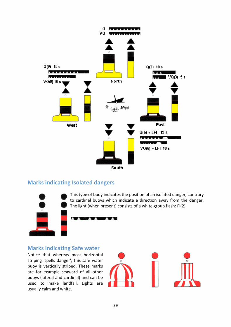
39
Marks indicating Isolated dangers This type of buoy indicates the position of an isolated danger, contrary to cardinal buoys which indicate a direction away from the danger. The light (when present) consists of a white group flash: Fl(2).
Marks indicating Safe water Notice that whereas most horizontal striping 'spells danger', this safe water buoy is vertically striped. These marks are for example seaward of all other buoys (lateral and cardinal) and can be used to make landfall. Lights are usually calm and white.

40
Special Buoys and Marks
We saved these buoys for last since they have not an actual navigation purpose. Most of the time these yellow buoys indicate areas used by navies or pipelines or surfing.
Range It is important to know at what distance (range) we may see a certain light, and when we can expect to lose sight of it, especially when making landfall. This range can be defined in several ways: Charted or Nominal Range: The nominal range is indicated in the chart next to the light or can be found in the Light List. This is the maximum distance at which a light may be seen at night based upon intensity and 10 nautical miles of visibility. Use the logo to navigate through this course.

41
Mathematics: Running fixes The som of angles in a triangle is 180° Let line DAE be parallel to line BC, then the angles α and α equal angles DAB and EAC, respectively. Therefore, the sum of angles in the triangle is 180° : a straight line.
“Doubling the angle” yields two equal angles So, α + δ + γ = 180° α + 180 ‐ β + γ = 180° 2α = β α + 180 ‐ 2α + γ = 180° 180° ‐ α + γ = 180° ‐α + γ = 0 γ = α
Two equal angles render an triangle isosceles In the triangle on the right, α = γ and β = 2α. By constructing the bisector h of angle β we create two little triangles in which x=y. Therefore, d1=d2. Next math chapter: Distance of horizon
α = 30° , β = 60° thus γ = 30°

42
Mathematics: Distance of horizon
Distance of horizon AD = h is the height of eye above the earth. DO = BO = CO = r (radius of the earth). Factum: any angle between a tangent line to a circle and the radius of the circle is a right angle. Since we have a right triangle ABO where AB = d, AO = h+r and BO = r, we can find a formula for d in terms of h: (AO)2 = AB2+BO2 (h+r)2 = d2+r2 d = sqrt[(h+r)2‐r2)], where r is approx. 3.440.1 nm An example: Let the eye height (h) be 4 meters (=0.0022nm); find the distance in nm of the geometrical horizon. d = sqrt[(0.0022 + 3.440.1)2 ‐ 3.440.12)] ; d = sqrt[11834303 ‐ 11834288] d = sqrt[15.146] ; d = 3.89 nm (geometrical) The distance of the visible horizon as found in the table is greater (4.2 nm) due to atmospheric refraction. The semi‐empirical function used is: d = sqrt[ (2x3440.1xh) / (1852xρo) ], where ρo accounts for refraction (0.8279).

43
Mathematics: Sextant angles
Vertical sextant angle The triangle OBL (see fig. below) can be described in terms of H, α and Distance: Distance = H/tan(α) The angle in rad. (0‐2π) and both height and distance in metres.
From rad. to degrees: α = A * π/180, 'A' being the same angle in degrees. To describe angle A in minutes total, then A*60 = a, thus α = (a/60) * (π/180). So, α = a/3438, 'a' being the angle in arc minutes.
FACTUM: tan(x) = x, if angle x is small. Resulting in (with π = 3.14): Distance (m)= H * 3438/a
Furthermore, distance in nm. = distance in meters/1852. Voilà, la very practical equation:
Distance = 1.856 * H/a
It contains just two approximations, both of neglitible influence. First, we left out the tan function and second we used 3.14 for π. Please realize that a smaller angle improves the approximation of the tan. Yet, as an opposing effect the instrument error of a smaller sextant angle increases. All in all, the factor 1.856 is not a typo, and just by chance near to the nautical mile: 1.852 kilometres. If you are still reading, you are very brave person and might perhaps agree that it originates from: (60 * 180)/(π * 1852). So far we considered a perfect triangle (OBL) and forgot that life isn't always perfect. Height h is usually quite small, but distance SB sometimes is not. This leads to an extra premise, which is seldom mentioned by other navigation textbooks: Angle OLS should be bigger than 15°.

44
In the beginning of the 19th century, sailors were describing wind forces instead of wind speeds, yet they lacks a uniform scale to estimate these forces. His scale as well as the more precise wind speeds in Knots or sometimes in meters per second are now widely used. Beaufort scale
Specification and speeds Equivalent speed at 10 m
above sea level
Mean Limits Description in forecasts
State of sea
Probable height of waves*
metres Force Description Specification for use at sea* knots metres
per second
knots metres per
second
0 Calm
Sea like a mirror. 0 0.0 <1 0.0‐0.2 Calm Calm 0.0
1 Light air Ripples with the appearance of scales are formed, but without foam crests. 2 0.8 1‐3 0.3‐1.5 Light Calm 0.1 (0.1)
2 Light breeze Small wavelets, still short but more pronounced. Crests have a glassy appearance and do not break.
5 2.4 4‐6 1.6‐3.3 Light Smooth 0.2 (0.3)
3 Gentle breeze
Large wavelets. Crests begin to break. Foam of glassy appearance. Perhaps scattered white horses.
9 4.3 7‐10 3.4‐5.4 Light Smooth 0.6 (1.0)
4 Moderate breeze
Large waves begin to form; the white foam crests are more extensive everywhere. Probably some spray.
13 6.7 11‐16 5.5‐7.9 Moderate Slight 1.0 (1.5)
5 Fresh breeze Moderate waves, taking a more pronounced long form; many white horses are formed. Chance of some spray
19 9.3 17‐21 8.0‐10.7 Fresh Moderate 2.0 (2.5)
6 Strong breeze
Large waves begin to form; the white foam crests are more extensive everywhere. Probably some spray.
24 12.3 22‐27 10.8‐13.8 Strong Rough 3.0 (4.0)
7 Near gale Sea heaps up and white foam from breaking waves begins to be blown in streaks along the direction of the wind.
30 15.5 28‐33 13.9‐17.1 Strong Very rough 4.0 (5.5)
8 Gale Moderately high waves of greater length; edges of crests begin to break into spindrift. The foam is blown in well‐marked streaks along the direction of the wind.
37 18.9 34‐40 17.2‐20.7 Gale High 5.5 (7.5)
9 Strong gale High waves. Dense streaks of foam along the direction of the wind. Crests of waves begin to topple, tumble and roll over. Spray may affect visibility.
44 22.6 41‐47 20.8‐24.4 Severe gale Very high 7.0 (10.0)
10 Storm Very high waves with long overhanging crests. The resulting foam, in great patches, is blown in dense white streaks along the direction of the wind. On the whole, the surface of the sea takes a white appearance.The 'tumbling' of the sea becomes heavy and shock‐like. Visibility affected.
52 26.4 48‐55 24.5‐28.4 Storm Very high 9.0 (12.5)

45
11 Violent storm
Exceptionally high waves (small and medium‐sized ships might be lost to view for a time behind the waves). The sea is completely covered with long white patches of foam lying along the direction of the wind. Everywhere the edges of the wave crests are blown into froth. Visibility affected.
60 30.5 56‐63 28.5‐32.6 Violent storm Phenomenal 11.5 (16.0)
12 Hurricane The air is filled with foam and spray. Sea completely white with driving spray; visibility seriously affected.
‐ ‐ 64 and over
32.7 and over
Hurricane force
Phenomenal 14.0 (‐)
* These columns are a guide to show roughly what may be expected in the open sea, remote from land. Figures in brackets indicate the probable maximum height of waves. In enclosed waters, or when near land with an offshore wind, wave heights will be smaller and the waves steeper.