Naval Research Laboratory Washington, DC 20375-5320

NRL/MR/7100--99-8373

The Art of Bond Graph Construction for Transducers

SAM HANISH

Acoustics Division

September 13,1999

Approved for public release; distribution unlimited.

DTICQUALnYINSpECTED4

19990915 OH

REPORT DOCUMENTATION PAGE Form Approved OMB No. 0704-0188

Public reporting burden for this collection of information is estimated to average 1 hour per response, including the time for reviewing instructions, searching existing data sources, gathering and maintaining the data needed, and completing and reviewing the collection of information. Send comments regarding this burden estimate or any other aspect of this collection of information, including suggestions for reducing this burden, to Washington Headquarters Services, Directorate for Information Operations and Reports, 1216 Jefferson Davis Highway, Suite 1204, Arlington, VA 22202-4302, and to the Office of Management and Budget. Paperwork Reduction Project (0704-0188), Washington, DC 20503.

1. AGENCY USE ONLY (Leave Blank! 2. REPORT DATE

September 13, 1999

3. REPORT TYPE AND DATES COVERED

4. TITLE AND SUBTITLE

The Art of Bond Graph Construction for Transducers

5. FUNDING NUMBERS

6. AUTHOR(S)

Sam Hanish

7. PERFORMING ORGANIZATION NAME(S) AND ADDRESS(ES)

Naval Research Laboratory Washington, DC 20375-5320

8. PERFORMING ORGANIZATION REPORT NUMBER

NRL/MR/7100-99-8373

9. SPONSORING/MONITORING AGENCY NAME(S) AND ADDRESS(ES)

Naval Research Laboratory Washington, DC 20375-5320

10. SPONSORING/MONITORING AGENCY REPORT NUMBER

11. SUPPLEMENTARY NOTES

12a. DISTRIBUTION/AVAILABILITY STATEMENT

Approved for public release; distribution unlimited.

12b. DISTRIBUTION CODE

A

13. ABSTRACT {Maximum 200 words)

The mathematical modeling of transducer by bond graphs possesses notable advantages. While these advantages come to true light in very complex devices, the method of bond graphs is applied here to elementary mechanical-acoustical-electrical devices, thus serving as an introduction to bond graph modeling procedures. The devices selected for illustration are (1) the longitudinal vibrator, (2) the electrodynamic microphone, (3) the moving armature transducer. In addition to these examples, a preview of 4-pole theory is presented to allow easy comparisons between bond graph modeling and conventional methods.

These notes are intended to accompany another publication entitled, "Monograph—Bond Graph Modeling of the Dynamics of Physical Systems," S. Hanish, Naval Research Laboratory, Washington, DC.

14. SUBJECT TERMS

Bond graphs Electrodynamic Microphone Longitudinal vibrator Moving armature transducer

15. NUMBER OF PAGES

27 16. PRICE CODE

17. SECURITY CLASSIFICATION OF REPORT

UNCLASSIFIED

18. SECURITY CLASSIFICATION OF THIS PAGE

UNCLASSIFIED

19. SECURITY CLASSIFICATION OF ABSTRACT

UNCLASSIFIED

20. LIMITATION OF ABSTRACT

UL

NSN 7540-01-280-5500 Standard Form 298 (Rev. 2-89) Prescribed by ANSI Std 239-18

298-102

CONTENTS

BULLETIN #1 - THE LONGITUDINAL VIBRATOR (A 2-Port Model) 1

BULLETIN #2 - ELECTRODYNAMIC MICROPHONE (Cascade Model) 7

BULLETIN #3 - TRANSDUCERS, GENERAL PRINCIPLES 12

BULLETIN #4 - THE ELECTROSTATIC TRANSDUCER (A 2-Port Model) 12

BULLETIN #5 - MATHEMATICAL MODELING OF ELECTROMECHANICAL TRANSDUCERS BASED ON ELECTRICAL FOUR-POLE THEORY 16

BULLETIN #6 - MOVING ARMATURE TRANSDUCER 21

in

THE ART OF BOND GRAPH CONSTRUCTION FOR TRANSDUCERS

Bulletin #1 - Longitudinal Vibrator (A 2-Port Model) (Ref.: F. Hunt "Electroacoustics" and S. Hanish "Treatise on Acoustic Radiation" Vol. IINRL)

The longitudinal vibrator can conveniently serve as a prototype in the art of bond graph construction.

Suppose first we have a moderately long thin elastic bar of constant cross sectional area and assume it is in steady state vibration at a fixed frequency. We propose to construct a bond graph model of this bar. Our procedure is outlined in a sequence of steps.

(1) As an initial step we perform a dynamic analysis of the motion of the bar. But immediately we note a different approach: in conventional analysis we formulate an equation of velocity resulting from applied force; in a different approach, because a bond graph pictures a flow of power, we seek to find the velocity at every point in the bar, as well as the force at every point, in terms of the force and velocity at one end of the bar. Let us set aside the physical causes of this force and velocity at the input point (that is, bar end). Because the bar is an elastic continuum the force and velocity at the second end are easily obtained. Analysis therefore leads to two equations relating forces F,, F2 and velocities V,, V2.

V^V.OvV,)

In most common applications' we find the functional relations to be linear, and the power variables decoupled, i.e.

F^A^ + BV, V^CF. + DV,

Here A,B,C,D apply only to the terminii of the bar. By so doing we have converted the bar description from that of a continuum to a system of 2 degrees-of-freedom, namely the velocities of the ends of the bar. On dimensional considerations it is seen that A,B,C,D are impedances, or admittances, or ratios of impedance's.

The above set of equations in F2, V2, obtained by dynamic analysis, has no relation to any preconceived model, be it electrical analogies or bond graphs, or signal graphs, or chose what one will.

(2) The second step in the procedure introduces modeling by bond graphs. To begin, one identifies each one of two degrees of-freedom with a "one-junction" (written as, -1-), and because these are coupled, the coupling (by bond graph rules) is a "zero-junction" (written as -0-). The primitive graph is then,

2| |4 |6

Manuscript approved August 10,1999.

The digits identify the power bonds, which are paths of power flow. Bonds #1, #7 are "inputs," that is "ports." Bonds #2, #4, #6 are reactive impedances or admittances associated with a lumped parameter 2 degree-of- freedom system. Bonds #3, #5 are interior coupling bonds. Completing a more elaborate graph, one has,

F, F2

Z2 Y4 Zs

V, F;

V, V,

The arrow directions are arbitrary, but it is advantageous to assign them "all right pointing," "all left pointing," or "symmetrical," (as above), Z,, Z6 are mechanical impendances, and Y4 is a mechanical admittance.

The above graph now permits writing of "graph equations" in accordance with the bond graph rules (1) that 1-junctions represent the operation of force summation, and (2) the O-junctions represent the operation of velocity summation. The "graph equations" are then:

(a) F, = Z2V, + F3; (b) V, = Y4F12 - V2; (c) F, = Z6V2 + F3

Here the coupling force F12 is the same as as F3.

By construction, the model has now three unknowns, namely Z,, Y4, Z6.

(3) The third, and crucial step in the construction of the bond graph model is to rearrange the "graph equations" so that they appear as the set,

F7 = GF, + HV,; V2 = JF, + KV,

in which G, H, J, K are algebraic functions of Z2, Y4, Z6, and are therefore unknown. To find them explicitly we return to the dynamic equations obtained by analysis, and equate comparable coefficients:

(a) G = A; (b) H = B; (c) J = C; (d) K = D

Because A, B, C, D are known, this set allows Z2, Y4, Z6 to be known function of one, two, three or all four of them.

The model, as a first approximation (i.e. 2 degrees-of-freedom) is now completed. It is seen to be a "one- zero-one" structure, that is, a conventional "Tee" in electric circuit theory which, in itself, is an approximation to a short transmission line. However it is to be emphasized that the bond graph model is independent of electric circuit or electric transmission line theory.

(4) The fourth step in the procedure is to introduce modal description of vibration of the bar by expanding Z2, Y4, Z6 in resonant or anti-resonant modes. This is possible because 7^, Y4, Z6 are transcendental functions of frequency. The type of expansion is optional. We choose here to expand Z2, Z6 in resonant modes, and Y4 in antiresonant modes. The bond graph symbols for expansions are "fans of bonds."

I, C2R, c?92 Cs 93 c' Ri R, \i/i3 G, r, \/ r2 \Ar3 \/ h

V„ VR\ V, Fa - ' Y'W I, v« I F^ F.j F3 hQ-Il S-i P- 7

V," V2 Vj1 v2

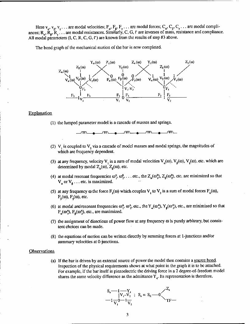
Here v0, vp, v ... are modal velocities; Fa, Fp, Fy... are modal forces; Co, Cp, Cy... are modal compli- ances; Ra, Rp, Ry... are modal resistances. Similarly, C, G, r are inverses of mass, resistance and compliance. All modal parameters (I, C, R, C, G, r) are known from the results of step #3 above.

The bond graph of the mechanical motion of the bar is now completed.

Y«(a» Z,(a» Z.(a» YT(a>) Z,(co) Zp(co) \y Yp(co) \y Zp(co)

z«((o) i y\ i y\ i \j 1 ,/ \Q 0 Q/ \J 1 l Va(cö)vß«°>/Vr(co) F«(m) ^/Vyi®) Va((D) Vp^v/co)

°F2 ^ }VrVi ?F4 N

F3 t" F3 __F3 A Fj F3 I Fs_ 1 *3 u n — — 1 lv v, u v2 l

Explanation

(1) the lumped parameter model is a cascade of masses and springs.

nnr\ 0 nnrv 9 rm\ # nff\ » nnr\—

(2) V, is coupled to V2 via a cascade of model masses and modal springs, the magnitudes of which are frequency dependent.

(3) at any frequency, velocity V, is a sum of modal velocities V0(co), Vp(co), Vr(co), etc. which are determined by modal Za(üö), Zß(co), etc.

(4) at modal resonant frequencies co* G$,... etc., the Za(co*), Zp(co*), etc. are minimized so that V or V„.. .etc. is maximized.

(5) at any frequency co the force F3(co) which couples V, to V2 is a sum of modal forces Fa(co), Fp(co), F/co), etc.

(6) at modal antiresonant frequencies co* co*, etc., the Ya(coA), Yp(coA), etc., are minimized so that Fo(coA), Fp(coA), etc., are maximized.

(7) the assignment of directions of power flow at any frequency co is purely arbitrary, but consis- tent choices can be made.

(8) the equations of motion can be written directly by summing forces at 1-junctions and/or summary velocities at O-junctions.

Observations

(a) If the bar is driven by an external source of power the model then contains a source bond. Inspection of the physical requirements shows at what point in the graph it is to be attached. For example, if the bar itself is piezoelectric the driving force in a 2 degree-of-freedom model shares the same velocity difference as the admittance Y4. Its representation is therefore,

Sc—1— Y4 /Z< |V,-V2 ; Se=SE—0

-1-0-1- \TF-

(b) Since the bar is an elastic continuum more points of velocity can be used in the dynamic analysis as needed. For example, if a compliance load is attached, x units of distance from the end its velocity V3 can be represented (in approximation) as the third degree-of-freedom in a 3 degree-of-freedom system, i.e.

(c) Since an elastic continuum may vibrate in several different modes—longitudinal, shear, twist, bulge, radial etc.—it is a common occurrence of a vibratory motion that two or more of these modes exist together over particular frequency ranges. Cross coupling between them is then to be expected. For example, suppose a vibration is simultaneously longitudinal, shear, and radial and assume the modeling makes the following assignments:

longitudinal mode: 2-d.o.f. (VJt,, VL2) shear mode: 2-d.o.f. (VS1, VS2) radial mode: 1-d.o.f. (VR)

(Note: d.o.f. means 'degree of freedom')

Assume further that analysis shows cross couplings of compliance, inertance, and resistance between respective velocities. An illustrative graph may have the following appearance:

1^'

0-C = vR—QMTF]] >1 äl /

\

t2S2 M4S2

MTF s V, L2

V, 's2

CRL, IRL2

CLJR CLJL, Q^S,

IL2R CL,L2 RL2SJ IL2S2I CL2S2

CS,L, Rs,L2 Csrs2

Is2L2» Cs2L,2 CS2Sl

Cross couplings modes are therefore easily made visible and tractable

An Alternative Approach

A 3-Port Model of a Longitudinal Vibrator

(1) As a first step we anticipate a model of the bar to have the character of a multiport representation. A port by definition is a location on the surface of the bar where power may enter or exit during motion of the bar. In bond graph theiry a port is pictured as a short straight line terminating at one end in a junction of the bond graph and directed at the other end away from the graph.

Inspection of the bar shows the existence of several possible ports. We chose three: one at each end of the bar, and one on the flat surface yb. Each port is identified by its power variables of effort and flow properly subscripted.

(2) A second step is to perform a dynamic analysis of the motion of the bar for the condition of steady state. The objective of this analysis is to associate with each port an explicit mathematical form of its input impedance or admittance. This procedure leads to a multiport solution of the motion of the bar.

(3) The next step is to construct an elementary bondgraph of the vibrating bar. Each port (in the form of a short straight line) is attached to a 1-junction, that is to an "effort divider." Since the motion at the ends are coupled to each other, their ports (here designated as A, B) are connected via aO-junction, that is, to an "effort divider." The flow of the third port, here designated as port C, is coupled to ports A, B only through the already established 0-junction. The primitive bond graph can now readily be constructed:

Port C \ h-, 1

PortB Port A

Here, the symbol hj is the input self admittance of port B, and of port A. The symbol h, is the input self admittance of port C.

(4) Since the bar in question is mechanical, its power variables are force F and velocity V. For various reasons the makers of models have found it advantageous to choose F to be "flow," and V to be "effort." A more complete bond graph incorporates these choices:

PortC h2 i

PortB

hi

1FW h2

VB

1 -0^ 1 Port A

(Note that arrow directions are arbitrary, but conform to convention.)

(5) We next formulate the constitutive equations relating force to velocity at each port. For the choice of effort and flow variables made earlier these are

(l)v =h,F;(2)v =h,Fh;(3)v =h,F

It is seen that h,, h, are mechanical admittances.

(6) Explicit forms of h,, h, are available in the literature (Ref. 1). Our next step is to incorporate them in the constitutive equations

(l)v=^f.. (2)vb=^-^„. (3)v =jhPsinH?) a j tan/wM b j tan/wM w J F v c '

L _ 1 v 1 . „2 _ E hF=ydxpcc= p

E= modulus of electricity (units: -^-1

p = mass of the bar per unit volume (units: N sec2/m4

(7) The bond graph model is now completed. For the choices of power variables it is seen to have the form of a "tee" (i.e. — 1 — 0 — 1 —)

(Ref. W.R Mason, "Physical Acoustics," Academic Press, New York, 1964.)

Example (a 3-port model of a quarter-wave resonator).

If velocity va is made zero by fixing end A of the bar in a wall, the graph constructed above takes on the form,

h2 hj

k k 0 1

PortB p v F PortC rb vw rw

Since the O-junction now has no exterior bond one sets Fb = Fw. The reduced graph is now,

hs h,

1- Port B F Port C

The admittances h,, h, are now in series, each having the flow Fw. They can be added to form h,

h = h1 + h2 = jhFsinM)+ 1 =jhFtanB) j hF tan ©

Setting v = v + vw (note that these v's are 'across' variables, that is 'efforts.') the graph is simplified to,

h v = h F.

1 Port B F Port C

Since h is a transcendental function it can be expanded in modes. We choose antiresonant modes, namely modes wherein at any as a sequence of antiresonant frequencies the 'across' variable (here velocity v) is maximized and the 'through' variable (FJ is minimized. The graph then becomes:

C(W.)

KWO-J^o vi

PortB

f PortC

o:

0, v3

,KW2)

-C(W2)

-I(W3)

C(W3)

= a quarter-wave longitudinal resonator

Other examples may be found in the cited references.

Tauchspulenmikrophone

Bulletin #2 - Electrodynamic Microphone (Cascade Model)

In the book "Grundlagen Der Sechnischen Akustik" by W. Reichardt,* there appears on page 305 a description of a Tauchspulenmikrophone (plunger spool microphone = electrodynamic microphone). Its essential parts are reproduced below.

Mshf

Electrodynamic microphone

Cross section of electrodynamic microphone

Here n, m, h are lumped compliance, mass, and resistance respectively.

♦Akademische Verlagsgesellshaf Geest Portig K. - G. Leipzig 1968

Acoustic Description

This device is an acoustic pressure receiver. Sound pressure incident from the left passes through screen b and protective grid w to reach the flexible diaphragm a to which a spool of wire is attached. Directly behind the diaphragm are a series of cavities and orifices which perform the function of smoothing the frequency response. The spool of wire is transverse to a static (d.c.) magnetic field created by permanent magnet c. In the rear cavity is an equalizer tube whose orifice f admits "atmospheric pressure" via tube feed g.

Bond Graph Model

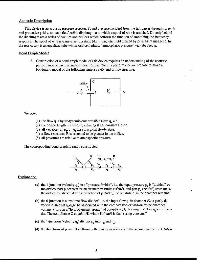
A. Construction of a bond graph model of this device requires an understanding of the acoustic performance of cavities and orifices. To illustrate this performance we propose to make a bondgraph model of the following simple cavity and orifice structure.

We note:

(1) the flow q is hydrodynamic compressible flow, q1 * q2

(2) the orifice length 1 is "short", meaning it has constant flow q, (3) all variables pp p2, q,, q2 are sinusoidal steady state. (4) a flow resistance R is assumed to be present in the orifice. (5) all pressures are relative to atmospheric pressure.

The corresponding bond graph is easily constructed:

Pi

R

PR P, Pi

\l\ TT-TOY

R

■1 „ PR1 ^1H^

Explanation

(a) the 1-junction (velocity qt) is a "pressure divider", i.e. the input pressure pt is "divided" by the orifice: part p: accelerates an air mass m (units NsVm5), and part pR (Ns2/m5) overcomes the orifice resistance. After subtraction of p, and pR the pressure p2in the chamber remains.

(b) the 0-junction is a "volume flow divider" i.e. the input flow q: in chamber #2 is partly di- verted in amount q^to be associated with the compression/expansion of the chamber volume acting as a "hydrodynamic spring" of compliance C, leaving exit flow q2 as remain- der. The compliance C equals 1/K where K (N/m5) is the "spring constant."

(c) the 1-junction (velocity q2) divides p2 into pR and pA.

(d) the directions of power flow through the junctions reverses in the second half of the sinusoi-

dal cycle, but not the directions of power flow in load elements I, R, C.

(e) the assignment of causality allows the formation of the constitutive equations for I, R, C:

(1) qr = \l pjdt (2) pR = RqR (3) P(. = i J q^t

B. We now proceed with the construction of the bond graph model. The component parts are,

(a) (forward) source (d) equalizing tube (b) diaphragm (e) (rear) source (c) (smoothing) orifices and cavities

(a) (forward) source Since the microphone is a pressure sensor we designate the exterior driver to be an "effort source" Se. Because of the presence of screen and grill we take the source impedance to be the acoustic resistanceR,.. To construct the bond graph of this source, the rule is invoked that an effort source has the operational significance of a 0-junction, and therefore must be followed by a 1-junction. The model is therefore,

R* R,

Se %

Pa

R has been added to account for radiation resistance, if not negligible.

(b) diaphragm The diaphragm is a mechanical component characterized by the power variables force F; velocity V . It is assumed in the first approximation to have rigid piston motion, featuring inertance Id, capacitance Ca, a resistance Rd. In operation the pressure difference between the opposing sides of this piston excite it into motion. The bond graph mode! is therefore an "effort divider," that is, a 1-junction:

U Cd

><• F«

Sc v„ ■1-

Rd

(c) (smoothing) orifices and cavities. For identification of chambers see subscripts on cross- section. The first cavity behind the diaphragm is designated by the symbol C2 (compliance #2). Volume velocity q^ enters and velocity qp exits. The bond graph model is therefore a "velocity divider," i.e. a O-junction,

Pc

qP

(d) the first orifice connects chamber #2 to chamber #3. Its volume velocity is qp. Pressure differences between the two sides of the orifice (tube) accelerate a mass m3 and overcome a resistance R3. The bond graph model is therefore an "effort divider" i.e. a 1-junction:

IT13 R3

I3 Rd

PN \ / /PR Pp -1- Pr

(e) the second chamber #3 has input volume velocity qß and exit velocity qy. Its model is there- fore a 0-junction:

P. p Pr

-0 %

(f) the second orifice connects chambers #3 and #4. Its graph is,

I R

Pr P8

(g) the third chamber #4 has input volume velocity qy and exit velocity % (= equalizer-tube velocity), the graph of which is,

Q

P*

-0- %

(h) the third "orifice" is the entrance and length the equalizer-tube in which the velocity by approximation is q^. Its graph is,

in Rf

I R \9» %/ ft\ / Pr

P5 _j. Pf

q5 q6

(i) (rear) source The rear source is the external acoustic pressure impinging on the surface aperture of the equalizer tube. Its graph is structurally the same as the forwarded source but has different magnitudes of the power variables and resistive loads.

Assembly of Components (Cascade Model)

In assembling the components of a bond graph one follows the simple rule that bonds having the same power variables coalesce into a single bond.

10

Assemblies can be made to various degrees of approximation. We sketch first an assembly which neglects

area transformations in the path of flow.

R,

PR>

1-

Rr Id <

'Pr P\C

Pa

Rd R

1- h Pc,

-0- PP 1- qs " q«=qs ~ % ' % qß

orifice between |—forward source—| diaphragm 1—chamber #2—|—■(^)ets #2 md #2—I

C I R C i' Rf

R R

-& 0 1- Ps

(%-<W

0- %

1- 1- p; qs'=q«

•s;

i_ . w„ I orifice between _i rhamhpr#4 |_equalizer_i rear 1 j-chamber#3-|-chambers#3and#4 | chamber#4 | (ube | soufce |

In a second approximation area transformation can be modeled by use of simple numerical ratio trans-

formers.

Electrical Output

Electrical output of the microphone is accomplished by Faraday induction. In this process the axial velocity Va of the diaphragm is imparted to the "spool" of wire so that the wire strands move normally to the (d.c.) magnetic flux B which is generated radially by a permanent magnet. By induction an e.m.f. appears

across the terminal of the spool of wire, length 1, of amount,

Eo.c = (VxB)J

For wire resistance RE the wire electrical current is i^EJR^. Since Eo is operationally an "effort" it has the character of a negative source (i.e. power output rather than power input). Its bond graph is then

RE

ER| BJv

Es:Se_^_i—Jpi_ÖY-5^; va= Y 1 1 »a °a

The port FE,Va is bonded to the 1-junction labeled q^.

Conclusion

The "plunger-spool" microphone has been modeled above as a lumped parameter device with all compo- nents in cascade. In practice the diaphragm will vibrate in multimode patterns of surface displacement. These can be modeled as a "fan of resonant modes" described in Ref. 2.

11

Bulletin #3 - Transducers, General Principles

In bond graph theory transducers are modeled as multiport systems in which the power variables of bonds are interrelated by coefficients arranged in matrices. For a system of n ports, in which the power variables of the I'th port are ei, fi (effort, flow), the interrelations are expressed by these matrix equations:

(a) to first (or linear) order in ej, fj:

n n ej = X Aij fj + X Bij ej, i = 1,2,... n

j=1 JA, n n

f, = X Cij fj + X Dij ej, i=l,2,...n

(b) to second (nonlinear) order in ej, fj:

n n n ej = X X Aijk fj fk + X X Bijkejek + X X Eijkfjek

j k j^in J k J k

n n n n n n fi = X X Cijk fj fk + X X Dijkejek + X X Fijkfjek

j k j k j k

Here, the quantities ei, fi on the Ih.s. are regarded as dependent variables, while ej, fr on the r.h.s. are taken to be independent variables. The rule for the selection of dependent variables is this:

(a) if an independent power variable is fj, the selected dependent variable is ej

(b) if an independent power variable is ej, the selected dependent variable is fj.

The ei, fi equations noted above are the canonical equations of classic theory. In drawing multiport transducers, the symbol TD is taken to be the bond graph structure of interlinked junctions, i.e. the interior system.

Bulletin #4 - The Electrostatic Transducer (A 2-Port Model) (Ref.: F. Hunt, "Electroacoustics")

The simplest embodiment of the electrostatic transducer is a parallel plate capacitor having a fixed separation d, a fixed charge qo, a fixed voltage Eo, and an area S. When a squeezing force is applied fluctuat- ing in magnitude and time, a flucutating charge q is induced by the changing separation distance x, thus generating a fluctuating voltage Ee. The interaction between mechanical and electrical variables is found to be nonlinear.

The Elementary Bondgraph

The electrostatic transducer under time varying input is modeled by transduction T with power variables Fe, x, and Ee, q:

F F ~f- T -y-; Fe = Fe(q); Ee = Ee(4*)

12

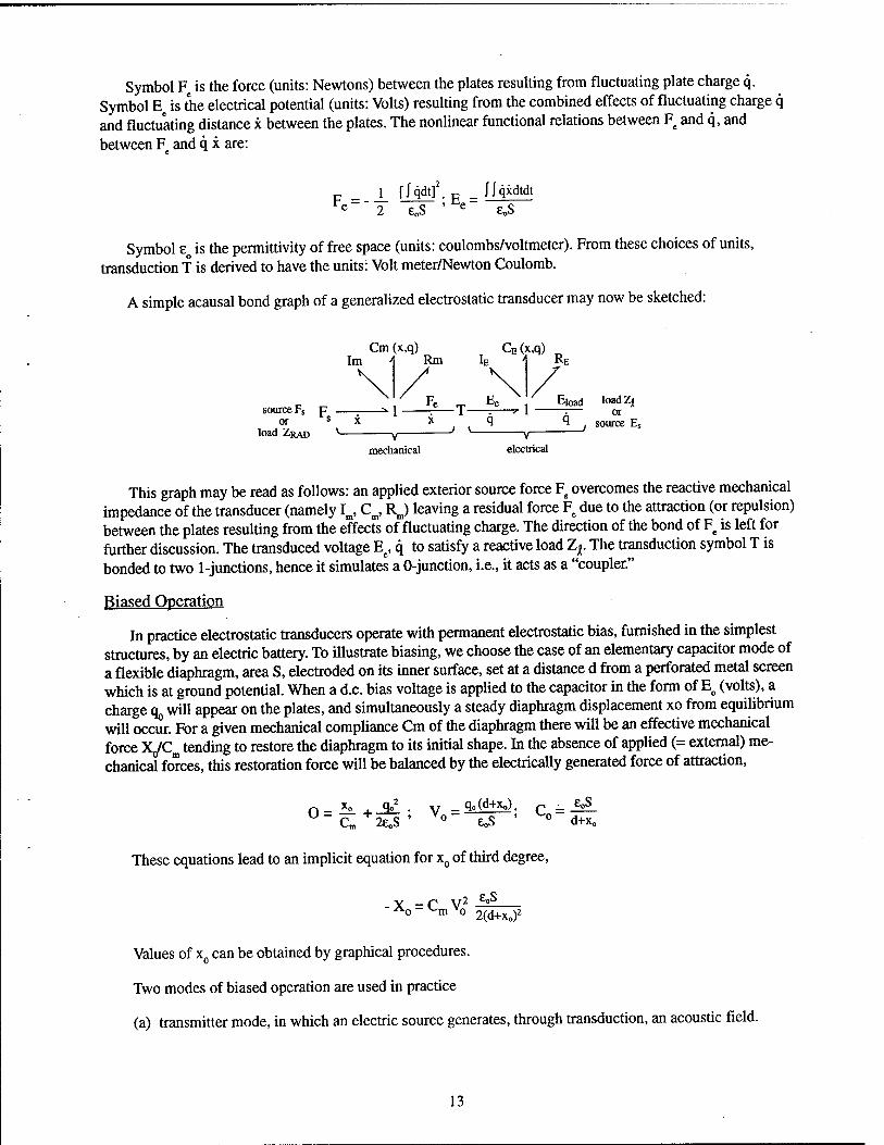
Symbol F is the force (units: Newtons) between the plates resulting from fluctuating plate charge q. Symbol Ee is the electrical potential (units: Volts) resulting from the combined effects of fluctuating charge q and fluctuating distance x between the plates. The nonlinear functional relations between F and q, and between Fe and q x are:

p _ J_ tfqdt]2. F = f/qxdtdt ***" 2 e„S ' e e0S

Symbol e is the permittivity of free space (units: coulombs/voltmeter). From these choices of units, transduction f is derived to have the units: Volt meter/Newton Coulomb.

A simple acausal bond graph of a generalized electrostatic transducer may now be sketched:

Cm(x,q) CE(x,q) Im A Rm IE RE

—. Eioad loadZi sources F . ^\ IS— T r^-^ 1 ™ or'

or s x X q q source E

load ZRAD V v ; * v

mechanical electrical

This graph may be read as follows: an applied exterior source force Fg overcomes the reactive mechanical impedance of the transducer (namely Im, CB, Rm) leaving a residual force Fe due to the attraction (or repulsion) between the plates resulting from the effects of fluctuating charge. The direction of the bond of Fe is left for further discussion. The transduced voltage Ee, q to satisfy a reactive load Zj.. The transduction symbol T is bonded to two 1-junctions, hence it simulates a 0-junction, i.e., it acts as a "coupler."

Biased Operation

In practice electrostatic transducers operate with permanent electrostatic bias, furnished in the simplest structures, by an electric battery. To illustrate biasing, we choose the case of an elementary capacitor mode of a flexible diaphragm, area S, electroded on its inner surface, set at a distance d from a perforated metal screen which is at ground potential. When a d.c. bias voltage is applied to the capacitor in the form of Eo (volts), a charge o^ will appear on the plates, and simultaneously a steady diaphragm displacement xo from equilibrium will occur. For a given mechanical compliance Cm of the diaphragm there will be an effective mechanical force XJCm tending to restore the diaphragm to its initial shape. In the absence of applied (= external) me- chanical forces, this restoration force will be balanced by the electrically generated force of attraction,

r\- X« _■_ i°2 . v _ q°(d+x<>). c - e„S Cm 2e0S ' ° e„S ° d+x«

These equations lead to an implicit equation for x0 of third degree,

- X = C V2 — ^o ^mvo 2(d+Xo)2

Values of x0 can be obtained by graphical procedures.

Two modes of biased operation are used in practice

(a) transmitter mode, in which an electric source generates, through transduction, an acoustic field.

13

(b) receiver mode, in which an acoustic field, acting as a mechanical source generates an electrical signal.

Restricting attention to the receiver mode, it is assumed that a fluctuating acoustic pressure acting over area S of the diaphragm is equivalent to a concentrated fluctuating force F,. Such a force generates a time fluctuating displacement X,, together with a time fluctuating charge q,. At any time then, total displacement X and total charge q are

X = d + X0 + X,;q = q0 + q1

Expanding q2 and qx, and neglecting second order terms, one finds the first order terms in fluctuating q, x( to be 2 q^ and q^. The forces and voltages of electromechanical coupling, to first order, namely F [read, mechanical force due to a fluctuating ql] and Eero(1) [read, electrical voltage due to fluctuating xj are

p _ goQi _ ~h . v _ qpX) _ V| . p _ €QS rmeW eoS "jwC»^«^1)" e«S ~jwCem'^

em~ q0

The units of CRM are m/V or C/N (meters/volt or coulomb/Newton). These expressions allow one to form acausal equations by use of the bond graph. At the 1-junction of the mechanical side of summation of forces on the diaphragm leads to F, = Zm v, ± F . The ambiguity in the sign of Fme(l) is resolved by noting that the time fluctuating charge ql acts as a source so that the force balance is F, + F = Zm vl5 from which

Fl = ff +Zm*i = -^ + ZmVl = Tme(1) + ZmVl

Here, T^. (which is 1/jco Cem) is the transduction coefficient. This choice of sign is justified on physical grounds. When Fj increases, closing the gap, the electrostatic force of attraction also increases; similarly, when F, decreases, opening the gap (between diaphragm and screen), the electrostatic force decreases. Thus, the fluctuation of charge appears on the mechanical side as a force source adding to the applied force F,. On the electrical side of transduction the electrical effect of gap motion in the form of displacement Xj is F,«n(i) = q0X1/e0S = X/Cem. This is the potential generated by the fluctuation Xr It's direction is away from the 1-junction labelled q, that is, it constitutes a negative source. In absence of an applied electric potential at the electrical terminals, summation at the 1-junction q leads to,

Z qi = Vme(i), Z = ZE + Zj, Zj = electrical load

In terms of first order fluctuating variables, this summation of potentials is,

Assume now that fluctuation in time is sinusoidal. By elimination of q, one finds

In absence of an electrical load, at low frequencies,

Z - 1 • Z. - 1 • <B_>0 J1" ^m <o->0 JUJ,~o

14

Thus as co -> 0,

Fi -^ll--FT-l-7^ o)->0 Cm

Here the quantity cm Ce/(^describes the coupling between mechanical and electrical 'compliances' at very low frequency. It is designated as k\ the coefficient of electromechanical coupling (squared),

Cm"I=i?'K " C?m '^°- dtxo'^em q0 Eo

These formulas show k2 to be a function of E0, c^, X0, and of diaphragm compliance Cm. From energy considerations there is a limit on the magnitude of k2,

k2 > 1

This is also a requirement for stability of the transducer. For given Cm the achievable bias displacement X0

is limited,

1 ^ Eo2eoS > Cm (dtx0);

It can also be deduced from these formulas that the low frequency electrical capacitance C', also called the 'free-running capacitance' is

C0' = -^., where C0 is the 'blocked capacitance.'

Equivalent Circuit: Ideal Transformer: Turns Ratio

Although every equivalent circuit may be transcribed into a bond graph, a bond graph is not, per se, an equivalent circuit. Steps required to form a 2-port equivalent circuit of an electrostatic transducer are outlined next.

(1) Let E , F, be the terminal electric potential and mechanical force respectively of the 2-port. On the electrical side the blocked electrical capacitance C0 is moved to 'shunt' position, that is, from a 1-junction to a 0-junction:

IE C0 RE IE RE CO

E, 1-1 • ^—1 0

The purpose of this move is to make C0 a 'coupler' between I, and v,.

(2) A ratio <)) is formed of the transduction coefficient Tem and Zg= 1/jco C0,

l/j(oCem=^ C0 N Y 1/jCO C0 Cem m V

15

This quantity is the "terms ratio" of an ideal electromechanical transformer which relates the independent variables I,, v, of the canonical equations to the dependent variables F,, E,:

E,4> = Fi; 1, = ^,; E1/I1 = F1/v,^,i.e. Z^Z^

In terms of the bias quantities E0, X0, o^,

V dl x0 dt x0

By shifting C0 to the shunt position, the mechanical compliance changes from cm to C^, a result of making the blocked capacitance C0 the coupling element.

The 2-port equivalent circuit is now complete: its bond graph is,

IE

E,

RE CO

1- l:f

0—-TF 0-

r

1 I. I.

The arrow directions are conventional for a 2-port electromechanical quivalent circuit.

Bulletin #5 - Mathematical Modeling of Electromechanical Transducers Based on Electrical Four-Pole Theory

(Ref.: "Grundlagen Der Technischen Akustik," W. Reichhardt, Leipzig, 1968)

In electrical 4-pole theory the power variables are E,, iv E2, ir Chosen as independent variables are E2, i2, which implies the functional relations,

Ei^.OV,)

To a first linear approximation, one finds,

Ei=Ani2+A12E2

or V

= A 3. ; A = Au A12

A A "21 22

In general all power variables are complex phasors in steady state operation, requiring (then) all coeffi- cients Aij to be complex numbers.

There are limits to the components Aij. These are set by the assumption that the transfer of power through the 4-pole is lossless. It is then seen that,

i(E1i?+ß!iI)-i-(E;i,+e;i,)=o

16

From this requirement one deduces that,

(a) (Au A2* + A * A21) i, i* = 0

(b) (A12A2*+A*A22)E2E*=0

(c) (A11A2*+A,;A21-l)i2E2=0

(d) (A12A2*+A*A22-l)i2E2 =0

Two types of transducers can be modeled by the El, il, equations noted above:

(1) El °c i2 for the (short circuit condition) E, = 0. In from (a) above A21, is purely imaginary (written j A11). A,, (at our option) is made purely real which makes A12 purely imaginary (written A£), as seen from (b). These assignments are inserted into (c) resulting in

A/jA^-jA^HAh + l,

(2) In the second type Ex« E2 for the (open circuited) conduct i2 = 0. In this case A12 is purely real (written A£,) because Ex is assumed purely real. From (b) above it is seen that A22 is purely imaginary (written A11). A21 (at our option) is made purely real, which from (a) above makes An purely imaginary (written j A^). These assignments inserted in (d) result in the formula

A.iAi-jAftjAä-1-O

or

jAftjA£-Ai!iAi = |A| = -l

This expression for the determinant of A, as well as the one in (1) above can serve to characterize electro- mechanical transducers.

Four-Pole Modeling of Electromechanical Transduction

The transduction component of a transducer can be modeled as a 4-pole. In bond graph rotation, the power variables Em, v, Fe appear as bonds,

i l Fe

E = electric field coupled to the mechanical circuit Fe = mechanical force coupled to the electrical circuit i = current v = mechanical velocity

Relations between variables are based on v, Fe, chosen as independent variables, and Em, i, as dependent variables.

E =AMv+A„F,

i = A2]v+A22F

Two types of transduction may be deduced.

17

(1) In the transfer term A12 v one sets v = 0. Then Em = An Fe. The determinant |A| = -1. This type of transduction characterizes the magnetic field transducer

(2) In the transfer term A2] v one sets v = 0. Then Em = A,, Fe. The determinant |A| = -1. This type of transduction characterizes the electric field transducer.

The transduction component is one link in a chain (= cascade) of transducer components, every link of which is itself a 4-pole.

Four-Pole Low Frequency Canonical Equations and Corresponding Bond Graphs

Magnetic Field Transducers

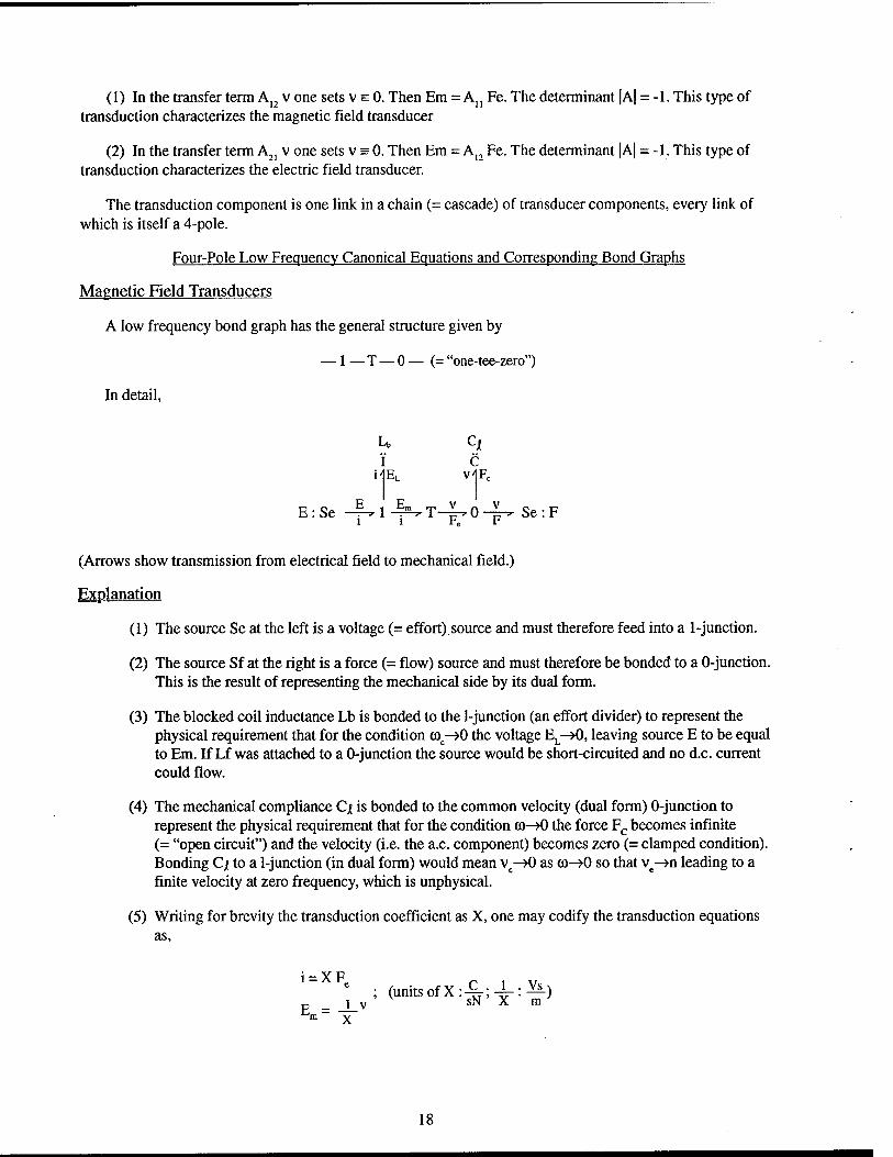
A low frequency bond graph has the general structure given by

— 1 — T — 0 — (= "one-tee-zero")

In detail,

Lb Cj I C

MEL v4Fc

E : Se -P- 1 -I^T^Uo -)U Se : F ii Fe F

(Arrows show transmission from electrical field to mechanical field.)

Explanation

(1) The source Se at the left is a voltage (= effort) source and must therefore feed into a 1-junction.

(2) The source Sf at the right is a force (= flow) source and must therefore be bonded to a 0-junction. This is the result of representing the mechanical side by its dual form.

(3) The blocked coil inductance Lb is bonded to the 1-junction (an effort divider) to represent the physical requirement that for the condition (0c-»0 the voltage EL-»0, leaving source E to be equal to Em. If Lf was attached to a 0-junction the source would be short-circuited and no d.c. current could flow.

(4) The mechanical compliance Q is bonded to the common velocity (dual form) 0-junction to represent the physical requirement that for the condition w->0 the force Fc becomes infinite (= "open circuit") and the velocity (i.e. the a.c. component) becomes zero (= clamped condition). Bonding Q to a 1-junction (in dual form) would mean vc—>0 as oo-»0 so that ve—>n leading to a finite velocity at zero frequency, which is unphysical.

(5) Writing for brevity the transduction coefficient as X, one may codify the transduction equations as,

e ; (units of X:^;-^:^) p _ 1 v sN X m bm~ X

18

The bond graph equations are found by summing voltage at the 1-junction and force at the 0-juntion,

E = jwLGi + ^v

i = X[^ + F] Ljw Cn J

Substitution of i into the E equation leads to the canonical set in v, F, whose matrix is,

A = /AAJA£\ A^ = ig-X + JL;jAÜ=jWL0X \jA21 A22 / Y

The determinant |A| = +1, as required.

Electric Field Transducers

A low frequency bond graph has the general structure given by,

— 0 — T — 0 — (= "zero-tee-zero")

In detail,

c c ME v4Fc

E E Sf —T-rO—:—7-T—g-^O c -" Sf * i im Fe F »

It is seen that the electrical field is in "direct form" and the mechanical field is in "dual form." The choice of dual form comes from the choice of v, F as independent variables.

Explanation

(1) The blocked capacity Cb is bonded to a 0-junction to represent the physical requirement that for the condition co->0 the current ic vanishes and the "supply current" i becomes the current ** coupled to the mechanical circuit.

(2) The source driving the blocked capacity must be a 'current source' Sf Ordinarily, this type of source is furnished by a 'voltage source' Se bonded to a 1-junction which is loaded with a source impedance Zs:

Zs ilEz

Ec E Sf = Se . ■> 1 . ' (= equivalent current source)

19

(3) Writing for brevity the transduction coefficient as Y, one may codify the transduction equa- tions as,

" Vim ; (units of Y : —; —: —)

'm ' y 1 v NYC

The bond graph equations are found by summing currents at the 0-junction and forces at the (dual) 0-juntion:

i=jwCbE+ -J- l_v y

E = YFe = YT^- + F] L iw Cm J LjwCm

Substitution of E into the i equation leads to the canonical set in v, F, whose matrix is,

Y /jAn Aii \. jA" = jWCn"'' A* = Y

\A21 jA22/ x Cb i . A21 = —— Y + — ; jA22 = jw Cb Y

The determinant |A| = -1, as required.

Conclusions

Modeling electromechanical transducers on the basis of electrical 4-pole theory involving the power variables E, i, v, F, leads to a set of canonical equations in which choices of independent variables must be made. For various reasons several authors choose v and F, with the additional choice of 'v across' and 'F through.' The mechanical branch is then represented in dual form. Other authors take i,v to be independent variables, both in direct form, namely 'i through', 'v through.' The resulting canonical set, while different from the set based on 4-pole theory, can be converted to it by interchange of variables.

Basic transducer types are simply summarized:

Magnetic field; — 1 — T — 0—; driven by a "voltage source" Electric field; — 0 — T — 0—; driven by a "current source"

Coefficient of Electromechanical Coupling and Its Effect on Low Frequency Properties of Inductance. Capacitance and Compliance-Case I. F. V at right angles to E. D or B. H.

The bond graph that describes the low frequency behavior of a magnetic field transducer calls for a blocked inductance Lb bonded to a 1-junction and a mechanical compliance bonded to a 0-junction (dual form). Because of electromechanical coupling the magnitude of the compliance depends on the nature of the electrical drive. Since magnetic field transducers are driven by a voltage source a purely (uncoupled) me- chanical magnitude of compliance can be measured by opening the electric input circuit. The open circuit compliance is then written a Q. When the circuit is closed and a current i flows through the (coil) inductance LG the open circuit compliance transferred to the electrical branch appears as coupled inductance Lc = Q./X2

bonded to the 1-junction. The sum Lb + Lc = Lr where Lf is the "free-running" inductance. By defining the coupling coefficient K2 = L/(Lc + Lb), it is readily deduced that the measured free-running inductance Lf = Lb/l-k

2. Further more it may readily be demonstrated that the measured compliance Ck on short circuit drive is related to the open circuited compliance Q by the formula, Ck= Q (1-k2). It also may readily be seen that because k2 < 1 the short circuit compliance is less than the open circuit compliance.

20

Similar considerations can be applied to electric field transducers. Since they are driven by a current source the mechanical compliance Ct is measured at electrical short circuit thereby bypassing the blocked capacity C.. When a drive voltage is restored the mechanical compliance decreases to the "free-running"

agnitude Q = Ck (1-k2). Correspondingly, the "free-running" electrical capacity Cf is increased to m Cf = Cb/l-k2.

Case II. F. v parallel to E. D or B. H

In this case negative compliances appear (see Bulletin on the electrostatic transducer). Summarizing the

changes to be made to Case I:

Electric field transducers

short circuit compliance Ck is replaced by open circuit compliance Q plus a negative compliance -

Q/k2;i.e.

—0— FeU F

Case I

-q/K

is replaced by -p— 0-p-

Casell

Magnetic Field Transducers

open circuit compliance Q is replaced by short circuit compliance Nk plus a negative compliance - Ck/k

2; i.e.

v

v n v

vV

v n v

-q/K /

p-0-p- is replaced by f^°~F~

Case I Case II

The rationale for these changes is explained by,

A. Lenk, Acoustica (1958) Nr. 3, page 159

Bulletin #6 - Moving Armature Transducer (Ref.: "Electric Circuits," MIT, J. Wiley & Sons, Inc., New York, 1943)

The Moving Armature Transducer (shown in the simplified sketch below) is based in operation on energy transfer between electrical and mechanical ports associ- ated with time variation of reluctance in a magnetic circuit. As shown it has three ports: (1) a field winding of electrical wire, Nf turns, around an iron yoke. Its power variables are potential difference vf (units: volt) and current if (units: amp.) (2) an armature winding of electrical wire, N turns, around the pivoted iron armature.

^A£U_^ *t

r<

NftarnJ]

=--?

n )Ntamsl

>ivot

i i -^ «-I—/\AS> o >+u

ature

itZJ f 5=area of gap^ +""

Moving-iron mechanism.

21

Its power variables are v (units: volt) and i (units: amp). (3) a mechanical port near the gap of the magnetic circuit. Its power variables are force F (units: newton) and velocity V (units: meter/sec).

In operation the gap energy Wm for a magnetic feed strength H (units: amp/meter) and magnetic flux density B (units: Vs/m2) is (HB/8ft) Sx = Wm, where Sx is the gap volume. When a force F is applied at the mechanical port, it changes the gap with x. The gap magnetic energy changes in the amount dW /dx = F. Allowing H = B/|io in the gap it is seen that F = SB2/8p [to.

At the electrical port of the field winding energy can only be extracted in the amount if d (Nf(p)/dt. The field current if is nearly constant and the flux <p (units: Vs), varying around a constant mean value, is also nearly independent of time to the approximation used in this analysis. Thus over time the field energy Wf at the field port does not change.

At the electrical port of the armature winding the rate of energy extraction when armature current i is active is dWa/dt = Nidcp/dt. Since current i is variable due to variable F, and flux cp in the gap varies with changing gap 8x, then energy may be transferred at the armature winding. The total flux in the gap is the sum of a constant component due to Nf if and a variable component Ni

47c(Nlif + Ni)Sti0 = ^SHoN^d + NP 9 (Xo + AX) Xo(l+AX/Xo)

If Ni/Nif and 5x/Xo are small relative to their squares, when the division is made and second order terms rejected the flux in the gap is approximated by

47cSnoNfif M _AX} T X0 Nfif X0

J

Since this flux varies with time and displacement there is a voltage v induced in the armature winding,

v = N^ = Lh- = Bf = — v (v = velocity) dt bdt fo X0

where Lb = l^toN2. B 4*£N* (units: Vs/m2) X0 ° -X.0

It is seen that Lb is the self-inductance of the armature winding. Thus the induced armature voltage has two components: the first in di/dt is the voltage of self induction, and the second an e.m.f. generated by mechanical motion.

It was noted earlier that the applied force in the magnetic circuit air gap is F = S B2/8ft fio, where B is the flux density. Noting that B = cp/S and rejecting (Ni/N^)2, (Ax/xo)2, (Ni/Njif) (Ax/xo), as terms of second order, it is seen that to first order,

2ft Sjlo (Nfif)2 n _ 2ft Ax + 2Ni...)

X2 ( X0 Nfif O

22

Each term in this 3-term form has significance. (1) the first term states that there is a component of force due to current if of fixed magnitude tending to close the gap. (2) the second term states that there is a negative component of force proportional to Ax which tends to increase the displacement, that is the application of this force widens the gap. (3) the third term states that there is a component of force that depends on armature current i, that is, when time varying current is is impressed in the armature ciruit it causes the armature to move in unison with it, and when the armature is moved by a mechanical force an e.m.f. in the electrical port is generated as noted above.

Construction of the Bond Graph (Ref.: Reichhardt, see above).

Since the field current if is virtually constant and the armature current i is variable with time some analysts combine their respective ports into one electrical port, the power variables of which are u (units: volt) and i cs (units: amp) where i es = if + i. We adopt this procedure here. Now the magnetic flux due to iFe is N4/ Rpe, where Rpe is the reluctance of the magnetic circuit (units: C/VS2). The input admittance of the combined electrical port"is Rp/j WNf

2 where Nf is the total turns of the field wire (units: none). The first element of the bond graph is a current divider (i.e. a 0-junction)

L, 'Fe

iFe

0 j - »RFe U—:— IFC- u jwNf

2

The second element of the graph involves the armature current i. At the gap the magnetic flux Ogap = NijioS/xo (units: VS). The drop in voltage across the gap is jffl NOgap or joo Lbi, Lb = N2 jioS/Xo. This is the input impedance of the current i. It's graph is a 1-junction:

(u-uw) - 1 uw • T • 1—— u-uw=jwLbi

i

The third element in the graph is the transduction. In electromagnetic circuits it is a gyrator, defined as the 'gyration' of electrical voltage (u) into mechanical velocity v (units: m/s), and the 'gyration' of electrical current into mechanical force F (units: Newton). Its graph is

!^Gy — "W V; W l

Fw

Here, UN is an 'across' variable and Fw is a 'flow' variable.

From earlier discussion,

SN , „ 47tNfifU0 / -. Vs — where Bf = ^2 (umts: _J_

and, X has the units of Vs/m.

23

The fourth element in the graph is the mechanical circuit. In this circuit is armature described dynamically by lumped parameters of mass M stiffness K mechanical resistance RM and radiation resistance R^j,. These are all attached to a flow (i.e. force) divider, which is a 0-junction:

RR

Here, FK, is the force of the negative stiffness discussed earlier.

The Completed Graph

electrical port

mechanical port

Application to the Telephone

In the telephone, the human voice supplies a variable pressure to a metal disphragm. This is the armature. It vibrates with a velocity which is transduced into an electrical current, which is transmitted to a distant receiver. At the receiver a voltage is generated upon reception of current. This voltage is transduced into a mechanical velocity of a diaphragm which radiates sound, completely reproducing the message sent by the transmitter.

24