nature methods: doi:10.1038/nmeth to 5 topological states indicated by the bold letters a, b, c, d,...

Nature Methods: doi:10.1038/nmeth.3209

Supplementary Figure 1

Graphical representations of kinetic model.

The linear unbound construct (a) has two free ligands (green). The two free ligands result in the receptor (red) binding with twice its solution on-rate (2*k1) to form the singly bound state (b). This now singly bound construct can either form a loop (c) by the same receptor binding to the second ligand at some loop closure rate (k2), or a second receptor can bind to the scaffold at the receptor solution-on-rate (k1) resulting an a doubly bound, or capped state (d).



Parallel measurements: biotin-streptavidin exploring a broad range of experimental conditions.

A highly parallel biotin-streptavidin off-rate measurement where an array of 16 different experimental conditions with 6 time points each were tested on a single 96-lane gel. Each of the 4 combs corresponds to a different salt condition, and within each comb experiments were conducted at 4 different temperatures. The band below the linear band is thought to be the result of enzyme promiscuity during the linearization process, and all lower bands result from the addition of a ladder used as a reference band to help alleviate the effects of pipetting error.


Temperature and salt dependence of biotin-‐‑streptavidin interaction kinetics. a) Eyring plot of the temperature dependence of the off-‐‑rate shows similar slopes for each salt condition but varyingoffsets. The off-‐‑rate and temperature were made dimensionless by scaling them by our reference units, i.e 𝑘!"" =

!!""!!!!

and

𝑇 = !!! . Fits were performed for data in the temperature range 25˚C to 50˚C Inset shows the temperature dependence of

the on-‐‑rates. Inset shows Eyring analysis of on rates over the same temperature range of 25˚C to 50˚C. From linear fits to these data we obtain a transition-‐‑state enthalpies of ΔHǂon = 9.48 ± 0.18 kcal/mol, and ΔHǂoff = 36.64 ± 0.50 kcal/mol b) Van’t Hoff plot from 25˚C to 50˚C. The dissociation constant was made dimensionless by scaling it by our reference units, i.e

. The red curve indicates a linear fit to the data. The fit was of the form ln !!!

= ∆!!− ∆!

!∙ !! , where R is

1.99 x 10-‐‑3 kcal K-‐‑1 mol-‐‑1, and T is the absolute temperature in K. This fit yielded the following values: ΔH = -‐‑26.01 ± 0.05 kcal mol-‐‑1, and ΔS = -‐‑0.0298 ± 0.0002 kcal K-‐‑1 mol-‐‑1. c) Plot showing salt dependence, again with similar slopes across all temperature conditions but with varying offsets. d) a 3D plot of the data fit with a least squares surface. All error bars represent the propagated error in the values taken from Supplementary Table 2.

Nature Methods doi:10.1038/nmeth.3209



Measurement of weak interactions.

The nanoswitches have proven very useful for the study of strong interactions. To extend the range of interactions which could be studied we modified the gel running procedure (see online methods). Noting that reptation of the DNA through the gel matrix acts as a quencher by preventing open loops from closing we are able to monitor the ratio of looped to unlooped as a function of time run in a gel. To indicate the location of the looped band a nanoswitch with a negligible off rate was run alongside each time point. A desthiobiotin-streptavidin-biotin (D-B) bridge was used for the weak interaction, and a biotin-streptavidin-biotin (B-B) bridge was used as the strong interaction. The B-B nanoswitches stayed relatively unchanged as a function of running time. The D-B constructs however show significant decay which was fit with a single exponential yielding a time constant of 35.3 ± 7.5 minutes.



Multistate band verification. To determine the location of the bands which represent the different states of the bispecific receptor binding to the trifunctionalized nanoswitch, we made nanoswitches capable of forming one or a subset of states (each set was run in triplicate). a) trifunctionalized nanoswitches without the bispecific receptor result in only a linear band (E). b) Nanoswitches with both digoxigenin functionalizations but lacking the biotin can form the E and D states. c) Nanoswitches lacking the terminal digoxigenin can form the E and C states. d) Nanoswitches lacking the central digoxigenin can form the E and B states. e) In this lane the samples from the lanes in b, c, and d were mixed in a 1:1:1 volumetric ratio before running on the gel to simulate the conditions seen in the multistate experiments. Note that it was not possible to make a construct which could exclusively form state A in Figure 3 but this state is attributed to the only remaining band, and selective quenching experiments (data not shown) indicate that this construct contains both digoxigenin and biotin dependent interactions which collapse into the appropriate states upon quenching exclusively with digoxigenin or biotin.



Multistate-model states. The model consists of 33 accessible states that can be occupied by the system. These 33 states are read out as 5 discrete gel bands, corresponding to 5 topological states indicated by the bold letters A, B, C, D, and E. A consists of only one state. Although bands B-D each represent one topological state, they are each composed of three states: 1) A piece of DNA in topological state B, C, or D that can


transition into topological state A, 2) A piece of DNA in topological state B, C, or D that cannot transition into topological state A, because the remaining ligand is capped by a second bispecific receptor, 3) A piece of DNA in topological state B, C, or D that cannot transition into topological state A because the DNA nanoswitch is missing the third ligand. The E state consists of 23 states. The boxes from top to bottom indicate linear states accessible when: all three ligands are present; the two digoxigenin ligands are present; the central digoxigenin ligand, and the biotin are present; the terminal digoxigenin ligand, and the biotin are present; only one ligand is present. This final set of three linear constructs, and the last construct in each box cannot form loops.



Multistate on-rate kinetic model schematic. The kinetic on-rate model consists of 3 solutions on rates and 6 effective loop concentrations resulting in effective on loop rate constants referred to as kbB, kbC, kd8C, kd8D, kd12B, kd12D, kbA, kd8A, and kd12A. The figure illustrates the kinetic model, excluding the capping phenomenon for clarity, and the table indicates the physical meaning and mathematical definition of each rate constant in the figure. The effective loop concentrations are as follows: LB is the effective concentration between the biotin on var 4 and the dig on var 12, LC is the effective concentration between the biotin on var 4 and the dig on var 8, LD is the effective concentration between the dig on var 8 and the dig on var 12, LBA is the effective concentration of the dig on var 8 relative to the var 4-var 12 complex, LCA is the effective concentration of the dig on var 12 relative to the var 4-var 8 complex, LDA is the effective concentration of the biotin on var 4 relative to the var 8-var 12 complex.

Supplementary Table 1: Comparison of biomolecular interaction analysis techniques


Supplementary Table 2: Comparison of our kinetic and thermodynamic values for the biotin-streptavidin interaction to those in previously-published works.


Supplementary Table 3: Kinetic and thermodynamic values obtained from studying the interactions of biotin with Streptavidin, Avidin, and Neutravidin. Errors indicate the 67% confidence interval on the fit parameters (a 3 parameter model fit to 6 data points for each condition).


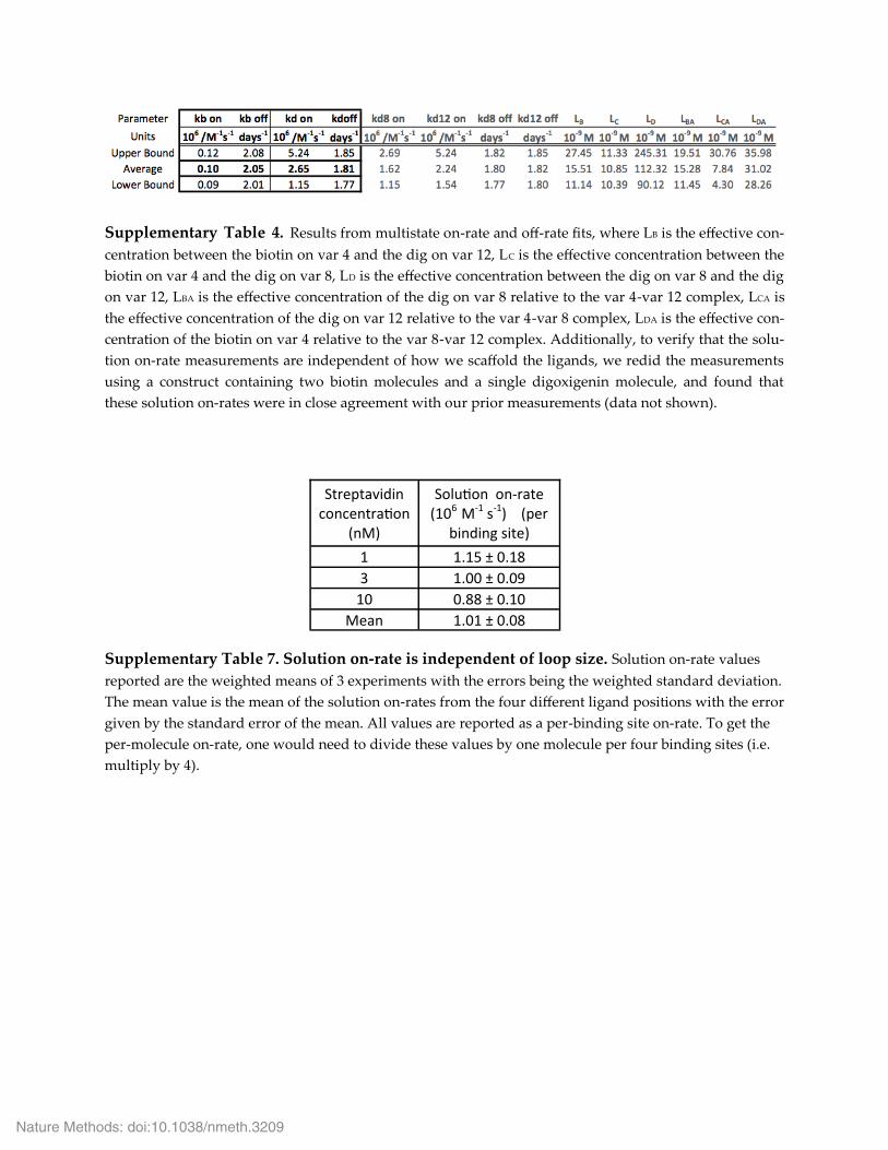
Supplementary Table 4. Results from multistate on-rate and off-rate fits, where LB is the effective con-‐‑centration between the biotin on var 4 and the dig on var 12, LC is the effective concentration between the biotin on var 4 and the dig on var 8, LD is the effective concentration between the dig on var 8 and the dig on var 12, LBA is the effective concentration of the dig on var 8 relative to the var 4-var 12 complex, LCA is the effective concentration of the dig on var 12 relative to the var 4-var 8 complex, LDA is the effective con-‐‑centration of the biotin on var 4 relative to the var 8-var 12 complex. Additionally, to verify that the solu-‐‑tion on-rate measurements are independent of how we scaffold the ligands, we redid the measurements using a construct containing two biotin molecules and a single digoxigenin molecule, and found that these solution on-rates were in close agreement with our prior measurements (data not shown).

Supplementary Table 7. Solution on-rate is independent of loop size. Solution on-rate values reported are the weighted means of 3 experiments with the errors being the weighted standard deviation. The mean value is the mean of the solution on-rates from the four different ligand positions with the error given by the standard error of the mean. All values are reported as a per-binding site on-rate. To get the per-molecule on-rate, one would need to divide these values by one molecule per four binding sites (i.e. multiply by 4).

Streptavidin concentra on

(nM)

Solu on on-rate (106 M-1 s-1) (per

binding site)

1 1.15 ± 0.18

3 1.00 ± 0.09

10 0.88 ± 0.10

Mean 1.01 ± 0.08


Supplementary Table 8. Solution on-rate is independent of receptor concentration. Solution on-rate values reported are the solution on-rate fit parameter from an error weighted fit of 10 data points with a 3 parameter model. The errors for measurements are the one-sigma confidence intervals of the fit parameter. The mean value is the mean of the solution on-rates from the three different concentrations with the error given by the standard error of the mean. All values are reported as a per-binding site on-rate. To get the per-molecule on-rate, one would need to divide these values by one molecule per four binding sites (i.e. multiply by 4).

Ligand Posi ons

Solu on on-rate (106 M-1 s-1) (per binding

site)

4-8 1.03 ± 0.15

8-12 1.34 ± 0.28

4-12 1.06 ± 0.29

1-12 1.75 ± 0.21

Mean 1.29 ± 0.17


Supplementary Note 1: Kinetic Models

Two-state kinetic model

For off-rate measurements of two-band systems, the data was fit to a single exponential decay-‐‑ing to zero. In the case of biotin-streptavidin measurements, the time constants were multiplied by two since each streptavidin has two pathways to cause the loop to dissociate. For on-rate measurements of two-band systems, we used a kinetic model consisting of 4 states and two ki-‐‑netic rate constants. Reverse rates were not considered to play a role since they were many or-‐‑ders of magnitude slower. This model results in a nonlinear system of differential equations that can be solved numerically (using NDsolve in Mathematica, for example). In our case, however, we were able to reduce these to a linear system of differential equations by using the assump-‐‑tion that the concentration of streptavidin is constant, which is a good approximation for our experimental conditions since the streptavidin was at a much higher concentration than the bio-‐‑tin-looped construct (3nM vs. 80pM). Furthermore, we validated this approximation by com-‐‑paring our results with the full numerical solution, and saw no discernable differences. Thus, the effective system of differential equations for the on-rate measurements is:

Where a(t) is the concentration of unlooped construct with no ligands bound, b(t) is the concen-‐‑tration of unlooped construct with only one ligand bound to one receptor, c(t) is the concentra-‐‑tion of looped construct with two ligands bound to a single common receptor molecule, d(t) is concentration of unlooped construct with both ligands bound to different receptor molecules, S is the concentration of streptavidin, and k1 and k2 are the per-site kinetic rates for streptavidin binding from solution and loop closure, respectively (accounting for the fact that in solution streptavidin has 4 binding sites, and after binding there are only 3 avaliable binding sites for loop closure). Note that k2 does not depend on the concentration of strepavidin in solution, since the loop closure rate is governed by an effective local concentration within the nanoswitch that is set by the loop length. This system of equations results in an analytical expression:

� �

)()()()(

)()()(2)()(2)(

1

2

21

1

tbkStdtbktc

tbktbtakStbtakSta

�� c� c

�� c�� c


C(t) was fit to the data with three free parameters, k1, k2, and Ao. In the regime of concentrations that we used (local biotin > free streptavidin > nanoswitches), the on-rate fi ing was less sensi-‐‑tive to k2 than k1, and constraining k2/k1 for the fits resulted in solution on-rates that overlapped within error with fits using k1 and k2 as free parameters.

This model allows for the determination of both the solution on-rate, which is independent of the polymer looping kinetics, and the loop closure rate as illustrated in Supplementary Figure 4.

Additionally, to examine the effect of ligand placement on the determination of the solution on-rate, we conducted biotin-streptavidin on-rate experiments with a variety of ligand positions at room temperature. The results, shown in Supplementary Table 7, indicate that the solution on-rate measurements are in reasonable agreement, exhibiting a relative standard error of the mean (1.29 x 106 M-1 s-1) of 13%.

To further test the robust nature of the system we analyzed the effect of keeping the ligand posi-‐‑tions constant while altering the concentration of the receptor (see Supplementary Table 8). We found that the measured solution on-rates are in reasonable agreement even when varying the receptor concentrations by an order of magnitude, yielding a relative standard deviation of 13%. Note that working outside this range may be difficult as protein concentrations become unreliable below 1 nM, and the rate of loop formation becomes very fast above 10 nM (see online methods for details).


Multistate off-rate model

For off-rate measurements of multistate (5 band) systems we used a model consisting of 5 topo-‐‑logical states and 3 rate constants. Reverse rates were not considered to play a role as the pres-‐‑ence of excess quencher prevents the closure of loops. This model results in a linear system of differential equations.

Where kb is the biotin off rate, kd8 is the off rate of the digoxigenin on var 8, kd12 is the off rate of the digoxigenin on var 12, A(0)-E(0) are the starting fractions of construct in each state A-E il-‐‑lustrated in Figure 3. These differential equations can be easily solved analytically (for example, using Dsolve in Mathematica), resulting in the following set of equations:

These equations were then fit to the data using fminsearch to minimize the chi-squared in MATLAB with kb, kd8, kd12, A(0), B(0), C(0), D(0), and E(0) as free parameters.


Multistate on-rate model

For the on-rate measurments of multistate (5 band) systems we used the model described be-‐‑low. This model results in a system of differential equations that can be solved numerically (using ODE15s in matlab, for example) with the following assumptions: The reverse rates were not considered to play a role since they were many orders of magnitude slower, and the concen-‐‑tration of the bispecific receptor is considered to be constant, which is a good approximation for our experimental conditions since the bispecific receptor was at a much higher concentration than the nanoswitches (3nM vs. 80pM).

The on rate model is schematized generally in the figures s5 and s6, followed by the differential equations that comprise the model.

Models were fit to experimental data using fminsearch in matlab to find the minimum of the χ2:

is the ith experimental data point. is the theoretical prediction given by the

model of the ith data point, and is the variance in the ith experimental data point.

To estimate errors on the fit parameters obtained using fminsearch, we calculated the local cur-‐‑vature of the χ2as a function of each fit parameter. The variance of the fit parameter is estimated

by where xi is the ith fit parameter.


Multistate on-rate model details

In addition to loop formation our model accounts for the presence of scaffolds that lack one or more ligand, and for the phenomenon of capping, in which two or more receptor molecules bind to a single scaffold. The model assumes that the concentration of the bispecific receptor molecule, S, is constant, as it is in great excess compared to the scaffold. Additionally, as the time scales for the on rate are much smaller than those for the off rate, the model assumes no unbinding events occur during loop formation.

Bold le ers A, B, C, D, and E represent topological states composed of the individual states, illustrated in figure s5, as follows:

A(t) = A(t)

B(t) = B(t) + Bk(t) + Bo(t)

C(t) = C(t) + Ck(t) + Co(t)

D(t) = B(t) + Dk(t) + Do(t)

E(t) = EA(t) + Eb(t) + Ed8(t) + Ed12(t) + Ebd8(t) + Ebd12(t) + Ed8d12(t) + Ek(t) + EBo(t) + Ed12Bo(t) + EbBo(t) + EBok(t) + ECo(t) + Ed8Co(t) + EbCo(t) + ECok(t) + EDo(t) + Ed12Do(t) + Ed8Do(t) + EDok

A linear piece of DNA that has all three ligands, and therefore has the ability to enter state A, is referred to as being in state EA.

Molecules can transition from state EA into either state Eb, Ed8, or Ed12 indicating a linear strand of DNA with a receptor bound to the biotin, var 8-dig, or var 12-dig respectively. Addi-‐‑tionally molecules can transition out of these states either by binding a second receptor, or by forming a loop as indicated by the following equations:

Eb’(t) = 4 kb S EA(t) – ( kd12B + kd8C ) Eb(t) – 2 kd8 S Eb(t) – 2 kd12 S Eb(t)

Ed8’(t) = 2 * kd8 * S * EA(t) – ( kbC + kd12D ) * Ed8(t) – 4 * kb * S * Ed8(t) – 2 * kd12 * S * Ed8(t);

Ed12)’(t) = 2 * kd12 * S * EA(t) – ( kbB + kd8D ) * Ed12(t) – 4 * kb * S * Ed12(t) – kd8 * 2 * S * Ed12(t);

Where kb, kd8, and kd12 are the per-site solution on rates for biotin, the dig on var 8, and the dig on var 12 respectively, and S is the concentration of the bi-specific receptor, assumed to be constant in time.


The formation of linear constructs with two receptor molecules bound can be modeled with the following equations:

Ebd8’(t) = 2 * kd8 * S * Eb(t) + 4 * kb * S * Ed8(t) – ( kd12D + kd12B + 2 * kd12 * S ) * Ebd8(t);

Ebd12’(t) = 2 * kd12 * S * Eb(t) + 4 * kb * S * Ed12(t) – ( kd8C + kd8D + 2 * kd8 * S ) * Ebd12(t);

Ed8d12’(t) = 2 * kd12 * S * Ed8(t) + kd8 * 2 * S * Ed12(t) – ( kbC + kbB + 4 * kb * S ) * Ed8d12(t);

Where Ebd8 indicates a linear scaffold with a receptor molecule bound to the biotin and a recep-‐‑tor molecule bound to the dig on var 8, Ebd12 indicates a linear scaffold with a receptor mole-‐‑cule bound to the biotin and a receptor molecule bound to the dig on var 12, Ed8d12 indicates a linear scaffold with a receptor molecule bound to the dig on var 8, and a receptor molecule bound to the dig on var 12

The linear EA state can also be capped by 3 separate receptor molecules.

Ek’(t) = 2 * kd12 * S * Ebd8(t) + 2 * kd8 * S * Ebd12(t) + 4 * kb * S * Ed8d12(t);

A linear piece of DNA that is missing one ligand cannot form state A. These linear pieces of DNA are referred to by the highest order loop they can form. Thus, a scaffold that only has a biotin on var 4 and a dig on var 12, and can therefore only form loop B, is referred to as EBo; a scaffold that only has a biotin on var 4 and a dig on var 8, and therefore can only form loop C, is referred to as ECo; a scaffold that only has a dig on var 8 and a dig on var 12, and can therefore only form loop D, is referred to as EDo.

Molecules can transition from state EBo into either state EbBo, or Ed12Bo indicating a linear molecule with a receptor bound to the biotin, or var 12-dig respectively. Additionally molecules can transition out of these states either by binding a second receptor, or by forming a loop as indicated by the following equations:

EbBo’(t) = 4 * kb * S * EBo(t) – kd12B * EbBo(t) – 2 * kd12 * S * EbBo(t);

Ed12Bo’(t) = 2 * kd12 * S * EBo(t) – kbB * Ed12Bo(t) – 4 * kb * S * Ed12Bo(t);

Molecules can transition from state ECo into either state EbCo, or Ed8Co indicating a linear molecule with a receptor bound to the biotin, or var 8-dig respectively. Additionally molecules can transition out of these states either by binding a second receptor, or by forming a loop as indicated by the following equation:

EbCo’(t) = 4 * kb * S * ECo(t) – kd8C * EbCo(t) – 2 * kd8 * S * EbCo(t);

Ed8Co’(t) = 2 * kd8 * S * ECo(t) – kbC * Ed8Co(t) – 4 * kb * S * Ed8Co(t);


Molecules can transition from state EDo into either state Ed8Do, or Ed12Do indicating a linear molecule with a receptor bound to the var 8-dig, or var 12-dig respectively. Additionally mole-‐‑cules can transition out of these states either by binding a second receptor, or by forming a loop as indicated by the following equation:

Ed12Do’(t) = 2 * kd12 * S * EDo(t) – kd8D * Ed12Do(t) – 2 * kd8 * S * Ed12Do(t);

Ed8Do’(t) = 2 * kd8 * S * EDo(t) – kd12D * Ed8Do(t) – 2 * kd12 * S * Ed8Do(t);

The following three equations represent scaffolds which have only two ligands, and become capped by the binding of two separate receptors.

EBok’(t) = 2 * kd12 * S * EbBo(t) + 4 * kb * S * Ed12Bo(t);

ECok’(t) = 2 * kd8 * S * EbCo(t) + 4 * kb * S * Ed8Co(t);

EDok’(t) = 2 * kd8 * S * Ed12Do(t) + 2 * kd12 * S * Ed8Do(t);

The rate of loop closure is described by the following equations.

A’(t) = kd8A * B(t) + kd12A * C(t) + kbA * D(t);

B’(t) = kd12B * Eb(t) + kbB * Ed12(t) – kd8A * B(t) – 2 * kd8 * S * B(t);

C’(t) = Eb(t) * kd8C + Ed8(t) * kbC – kd12A * C(t) – 2 * kd12 * S * C(t);

D’(t) = Ed8(t) * kd12D + Ed12(t) * kd8D – kbA * D(t) – 4 * kb * S * D(t);

Where kbB is the rate of biotin binding to form state B, kbC is the rate of biotin binding to form state C, kd8C is the rate of dig binding to var-8 form state C, kd8D is the rate of dig binding to var-8 form state D, kd12B is the rate of dig binding on var-12 to form state B, kd12D is the rate of dig binding on var-12 to form state D.

Loops which could transition into state A but are capped by having a second receptor molecule bind to the remaining ligand can be described as follows:

Bk’(t) = 2 * kd8 * S * B(t) + kd12B * Ebd8(t) + kbB * Ed8d12(t);

Ck’(t) = 2 * kd12 * S * C(t) + kd8C * Ebd12(t) + kbC * Ed8d12(t);

Dk’(t) = 4 * kb * S * D(t) + kd12D * Ebd8(t) + kd8D * Ebd12(t);

Where Bk, Ck, and Dk are the capped versions of Loops B, C, and D respectively.


A linear piece of DNA that is missing one ligand cannot form state A. These linear pieces of DNA are referred to by the highest order loop they can form. Such that a scaffold that only has a biotin on var-4 and a dig on var-12, and can therefore only form loop B, is referred to as EBo; a scaffold that only has a biotin on var-4 and a dig on var-8, and therefore can only form loop C, is referred to as EBo; a scaffold that only has a dig on var-8 and a dig on var-12, and can therefore only form loop D, is referred to as Edo.

Bo’(t) = kd12B * EbBo(t) + kbB * Ed12Bo(t);

Co’(t) = kd8C * EbCo(t) + kbC * Ed8Co(t);

Do’(t) = kd12D * Ed8Do(t) + kd8D * Ed12Do(t);

Given these equations the amount of EA, EBo, ECo, and EDo can be described as follows:

EA(t) = EA_Start – Eb(t) – Ed8(t) – Ed12(t) – A(t) – B(t) – C(t) – D(t) – Ebd8(t) – Ebd12(t) – Ed8d12(t) – Ek(t) – Bk(t) – Ck(t) – Dk(t);

EBo(t) = EB_Start – EbBo(t) – Ed12Bo(t) – Bo(t) – EBok(t);

ECo(t) = EC_Start – EbCo(t) – Ed8Co(t) – Co(t) – ECok(t);

EDo(t) = ED_Start – Ed12Do(t) – Ed8Do(t) – Do(t) – EDok(t);

Multistate Kinetics Results:

Fi ing the data with these on-rate and off-rate models, and using fminsearch to reduce the chi squared yielded the values reported in Supplementary table 4 for the fit parameters.


Supplementary Note 2: Semiempirical formula for temperature and salt

dependence

The temperature and salt dependence were analyzed using Eyring analysis and kinetic salt effect theory, respectively9 (Supplemental Figure 1). Empirically, we found that these depend-‐‑encies were separable over our measurement range, giving the following expression for the off-rate of DNA-linked biotin from streptavidin as a function of salt (25mM-500mM) and temper-‐‑ature (25˚C-50˚C):

where koff is the value of the off-rate in s-1, T is the value of the absolute temperature in K, and I is the value of the ionic strength of the solution in mM. From a 2D least squares fit of our data, we found an offset A of 42.41 ± 1.7, an enthalpic prefactor B of -1.83 ± 0.06 x 104, and a salt de-‐‑pendence C of -0.033 ± 0.01. We note that the off rates used in developing this formula match off rates measured using a radiolabeled biotin-functionalized oligo under similar conditions, and are slower than the off rates measured using a free biotin.

��

lnkoffT

§�

©�¨�

·�

¹�¸�| A �

BT�C I


Preface:

This document serves as a detailed protocol to provide you with all the information

needed to implement the nanoswitch platform in your lab. The protocol will walk you through

all the steps required to form nanoswitches, and use them to make on-rate and off-rate

measurements. The protocol goes through the specific steps required to make measurements on

the ubiquitous biotin-streptavidin system, with notes about where changes can be made to

adapt the platform to your system of interest. While supplies last, we are happy to provide a

starter kit, which contains all of the oligonucleotides needed to perform these measurements, to

any interested labs. The detailed contents of the kit are described in section 2 of this protocol.

Anyone interested in obtaining a starter-kit for their lab should visit

http://wonglab.tch.harvard.edu/nanoswitch/ .

Protocol:

1. Linearizing the M13 Scaffold

To begin one must first prepare the linear single-stranded M13 scaffold. We do this by using

a synthetic oligonucleotide complementary to the site where we want to cut that creates a

double stranded region allowing the restriction enzyme BtsCI to cleave the M13 scaffold. The

following will walk you through the procedure needed to make the linear scaffold.

Note: We recommend using Eppendorf LoBind tubes and Corning DeckWorks Lowbind Tips

(Corning Product #s: 4121 and 4147) for all liquid handling.

1.1 Reagents needed:

1.1.1 250μg/ml (~100nM) Circular single-stranded M13 DNA (New England Biolabs

Catalog#: N4040S)

1.1.2 100μM Synthetic oligonucleotide complementary to the BtsCI restriction site

(sequence 5’->3’: CTACTAATAGTAGTAGCATTAACATCCAATAAATCATACA).

1.1.3 BtsCI (20,000 units/ml) Restriction Enzyme (New England Biolabs Catalog#: R0647S

or R0647L)

1.1.4 10x NEBuffer 2 (New England Biolabs Catolog #: B7002S)


http://wonglab.tch.harvard.edu/nanoswitch/

Mounir Koussa

Supplementary Protocol

1.1.5 Nuclease Free Water (Invitrogen Ultrapure Distilled Water DNAse and RNAse free

Catalog # 10977-015)

1.2 Mix the following in a PCR tube (Axygen PCR-02D-C)

1.2.1 ____ 5μl of 100nM circular single-stranded M13 DNA

1.2.2 ____ 2.5μl of 10x NEBuffer 2

1.2.3 ____ 0.5μl of 100μM BtsCI restriction-site complimentary-oligonucleotide

1.2.4 ____ 16μl of Nuclease Free Water

1.2.5 ____ Pipette to mix thoroughly being sure to avoid air bubbles

1.3 ____ Place the tube in a thermocycler and subject to the following linearization protocol:1

1.3.1 ____ Bring to 95° C and hold for 30 seconds

1.3.2 ____ Cool to 50° C

1.3.3 ____ Add 1μl of the BtsCI enzyme

� Mix thoroughly with a pipette to ensure enzyme is well mixed. The enzyme

is in glycerol and will sink to the bottom if not mixed well. It is best to use a

pipette set to ~10μl to do this as the 1μl pipette may not provide adequate

mixing. Failure to do this may greatly lower linearization efficiency.

1.3.4 ____ Allow the mixture to sit at 50° C for 1 hour

1.3.5 ____ Bring the mixture up to 95° C for 1 minute to heat deactivate the enzyme

� For convenience you may want to set the thermocycler to hold at 4°C after

completion

1.3.6 This will result in 25μl of ~20nM linearized circular M13 in NEBuffer 2

� We have scaled this up as much as 4 times resulting in 100μl of final product

with no obvious reduction in linearization efficiency

� Additionally we have found the linearization to be equally efficient in

NEBuffers 2, 2.1,4, and cutsmart

� To aid in quantification the linearized DNA can be spiked with 1 μl BstNI

Digest of pBR322 DNA (New England Biolabs). This provides low molecular

weight bands which can be used as intensity references to combat errors in

pipetting at later stages


Now that linear single-stranded scaffold is made you will need the set of oligonucleotides that

are complementary to the scaffold. We have chosen to use 60 nt oligonucleotides. This yields

120 60 nt oligonucleotides and one 49 nt oligonucleotide. We have divided these

oligonucleotides into two groups to avoid having to mix 121 oligonucleotides for each

construct. A mixture of 12 oligonucleotides evenly spaced along the backbone are each stored in

their own tubes and referred to as variable regions or Vars. The remaining 109 oligonucleotides

are all pre mixed together and we refer to these as backbone oligonucleotides. We have created

a SnapGene DNA file which has these regions highlighted and labeled (in the SnapGene file, the

bottom strand is the M13 sequence while the top strand represents the oligonucleotide

sequences). SnapGene Viewer is freely available software that can be downloaded at:

http://www.snapgene.com/products/snapgene_viewer/ . Images exported from SnapGene can

be found below. The SnapGene file can be found at: https://drive.google.com/file/d/0B_Sa-

wyS5qEUaldiUFlGbHkwczQ/view?usp=sharing , an excel file with the 109 backbone

oligonucleotides can be found at: https://drive.google.com/file/d/0B_Sa-

wyS5qEUcEF3OF9ZQkRTeWM/view?usp=sharing , and an excel file with the 12 variable

oligonucleotides can be found at: https://drive.google.com/file/d/0B_Sa-

wyS5qEUbTVHdUp6V0NUUjQ/view?usp=sharing.c Additionally, these files are available in

the online supplementary materials on nature method’s website.


https://drive.google.com/file/d/0B_Sa-wyS5qEUaldiUFlGbHkwczQ/view?usp=sharing

https://drive.google.com/file/d/0B_Sa-wyS5qEUaldiUFlGbHkwczQ/view?usp=sharing

https://drive.google.com/file/d/0B_Sa-wyS5qEUcEF3OF9ZQkRTeWM/view?usp=sharing

https://drive.google.com/file/d/0B_Sa-wyS5qEUcEF3OF9ZQkRTeWM/view?usp=sharing

https://drive.google.com/file/d/0B_Sa-wyS5qEUbTVHdUp6V0NUUjQ/view?usp=sharing.c

https://drive.google.com/file/d/0B_Sa-wyS5qEUbTVHdUp6V0NUUjQ/view?usp=sharing.c

Linearized M13 showing the 12 evenly spaced Var 1-Var 12(orange) oligonucleotides

interrupted by 11 back bone regions (green), each of which is filled with 10 backbone

oligonucleotides (maroon) (with the exception of backbone region 1 which only has 9 backbone

oligonucleotides). In the following image we have zoomed in on the region between Var 3 and

Var 4.


2. Materials available upon request:

To facilitate trying the nanoswitch platform in your lab, we have ordered some materials for

starter kits that we will provide while supplies last. We will provide a mixture of the 109

backbones, a mixture of the 10 Vars (Vars 1, 2, 3, 5, 6, 7, 9, 10, 11, and 12), and a mixture of Var

4-3’biotin and 5’biotin-Var 8. The 109 mix can be used in conjunction with the provided Var

oligos to create scaffolds capable of forming loops between Vars 4 and 8 upon the addition of

streptavidin. Additionally, one could use the 109 mix in conjunction with 12 separately

purchased Var oligonucleotides (or the 10 var mix and separately purchased Var 4 and Var 8

oligonucleotides) which can be functionalized to your specific needs. Protocols for

functionalizing oligonucleotides for incorporation into this scaffold can be found in Halvorsen

et. al 2011 and Koussa et. al 2014.

Below we provide a protocol for using the included 109 mix, the 10 Var Mix, and the mix of the

two biotinylated oligonucleotides, to make biotin-SA on-rate and off-rate measurements.


3. Building the construct:

3.1 Hybridize the 121 oligonucleotides to the scaffold

3.1.1 ____ Hydrate provided oligonucleotides

3.1.2 ____ Hydrate the 109 backbone oligonucleotide mixture with nuclease free water to

achieve a total oligonucleotide concentration of 100μM (10μl per nanomole).

3.1.3 ____ Hydrate the 10 var mixture with nuclease free water to achieve a total oligo

concentration of 100μM (10μl per nanomoles).

3.1.4 ____ Hydrate the mixture of the two biotinylated vars with nuclease free water to

achieve a total oligonucleotide concentration of 100μM (10μl per nanomoles)

3.1.5 ____ Create a mixture of 119 unfunctionalized oligonucleotides

� To help ensure that each scaffold has all of its oligonucleotides hybridized we

recommend putting the oligonucleotides in at a 10 fold excess to the scaffold.

As having many excess biotinylated oligonucleotides would be costly and

problematic for on-rate experiments, the biotinylated oligonucleotides will

only be put in at a 4x excess to the scaffold. As all of the oligonucleotides are

mixed in an equimolar fashion, adding 1.09 μl of the 109 mixture is simply

like adding 0.01 μl of each of the 109 oligonucleotides at 100μM.

3.1.6 ____ Mix the following in an Eppendorf DNA LoBind tube (0030 108.035)

a. ____ 10.9μl of the 100μM 109 backbone mix

b. ____ 1.0 μl of the 10 Var mixture

3.2 Mix the single stranded scaffold, unfunctionalized oligonucleotides, and functionalized

oligonucleotides

3.2.1 Mix the following in an Axygen PCR tube

a. ____ 5μl of 20nM linear single-stranded M13 DNA (see Section 1 )

b. ____ 1.19μl the mixture of 119 unfunctionalized oligonucleotides

� This is essentially like adding 0.01 μl of each oligonucleotide at 100μM which

gives a 10 fold excess to the 5μl of 20nM scaffold


c. ____ 0.8 μl of 100x dilute biotinylated Var mixture (1μl of the mixture of

functionalized Var 4 and Var 8 + 99μl of nuclease free water)

� This is essentially like adding 0.004 μl of each of the biotinylated Vars at

100μM thus giving a 4 fold excess compared to the scaffold

d. ____ 0.22 μl of 10x NEBuffer 2

e. ____ Pipette to mix thoroughly

3.2.2 Place the mixture in a thermocycler and subject it to the following protocol

a. ____ Heat the sample to 90° C

b. ____ Cool the sample 1°C per minute until it reaches 20°

� Note: if non-thermostable custom functionalized-oligonucleotides are

used these oligonucleotides should not be added in until after the mixture

has reached a temperature compatible with the functionalized

oligonucleotide

� For convenience you may want to set the thermocycler to hold at 4°C

after completion

3.3 Optional PEG precipitation step to remove excess oligonucleotides.

Large pieces of DNA such as the scaffold will precipitate out, while smaller pieces of DNA such

as the oligonucleotides will remain in the supernatant. (This is not necessary for the biotin-

streptavidin experiments but may be useful for custom applications).

Note: that the precipitation efficiency is very sensitive to the concentration of the PEG so it helps

to make a large stock of PEG that you can calibrate so that you do not have to calibrate your

concentration every time you make a new PEG stock

3.3.1 Make a 30% (by weight) stock of 8k PEG (Polyethylene Glycol 8000 Amresco 0159-

500G)

a. ____ Add 15g of 8k PEG to a 50 ml falcon tube

b. ____ Bring this up to 50 ml with nuclease free water


3.3.2 Make 2 dilutions of your PEG stocks in protein LoBind tubes as follows (As

mentioned above, the efficiency is very sensitive to PEG concentration thus the

following percentages may not work for you and you may have to tweak the

percentages for your 30% stock

a. 4.75% PEG in 30mM MgCl2 (This is higher so that when mixed with the 40μl of

DNA the final PEG concentration will be ~3.5%)

i. ____ 38 μl of 30% PEG stock

ii. ____ 24 μl of 300mM MgCl2

iii. ____ 178 μl of nuclease-free water

b. 3.5% PEG in 30mM MgCl2

i. ____ 28 μl of 30% PEG stock

ii. ____ 24 μl of 300mM MgCl2

iii. ____ 188 μl of nuclease-free water

3.3.3 Dilute your hybridized construct to 40 μl in 30mM MgCl2 in a DNA LoBind tube

� For example, if you have 8 μl of the hybridized DNA/oligonucleotide

mix then to this mix you should add 4 μl of 300mM MgCl2 and 28 μl

of nuclease-free water

3.3.4 Perform the PEG precipitation

a. ____ Add 115 μl of 4.75% PEG and mix thoroughly

b. ____ Centrifuge at 16,000 rpm for 30 minutes at room temperature

c. ____ Carefully remove the top 145 μl

� This should be done very carefully as it is easy to disturb the pellet it

should take roughly 30 seconds to slowly pipette out the supernatant in

one smooth draw. It helps to constantly be pipetting near the fluid air

boundary as to be as far away from the pellet as possible

d. ____ Add 115 μl of 3.5% PEG and mix thoroughly

e. ____ Centrifuge at 16,000 rpm for 30 minutes at room temperature


f. Carefully remove the top 115 μl





g. ____ Add 115 μl of 3.5% PEG and mix thoroughly

h. ____ Centrifuge at 16,000 rpm for 30 minutes at room temperature

i. ____ Carefully remove the top 115 μl





j. The remaining 10 μl should have the hybridized DNA scaffold free of any

detectable amount of free floating oligonucleotides

This construct is now ready for use in on-rate experiments.


4. On-rate Experiments:

To avoid the formation of aggregates (streptavidin molecules linking multiple scaffolds) we

work at low construct concentrations (i.e. the concentration of the construct should be lower

than the effective concentration of the two biotins on the scaffold, which in the case of Vars 4

and 8, is ~30nM. The construct prepared in the above protocol (3.2) is at a concentration of

~16nM. To ensure that aggregation is not an issue we will dilute this 100 fold.

4.1 Dilute the construct 100 fold to achieve a concentration of 160 pM. (note if you used

oligonucleotides at lower concentration your construct may already be less concentrated

than 16nM if you used different volumes in creating your construct you must calculate the

final construct concentration)

4.1.1 ____ In an Eppendorf protein LoBind tube(0030 108.094), mix 1μl of your construct

with 99μl of the buffer in which you wish to do the experiment

One buffer condition that we recommend for biotin streptavidin experiments is 1x

NEBuffer 2 supplemented with an additional 150mM NaCl (total 200mM NaCl)

4.1.2 To make 2 ml of this mix the following

a. ____ 200 μl of 10x NEBuffer 2

b. ____ 100 μl of 3M NaCl in nuclease-free water

c. ____ 1,700 μl of nuclease-free water

To avoid capping (i.e. the binding of two streptavidin molecules to one construct thus rendering

that construct unloopable) the streptavidin concentration should also be well below the effective

concentration of the ligands on the scaffold which for Vars 4 and 8 is ~30nM. To achieve this we

will dilute the streptavidin to ~6nM so that when mixed in equal volumes with the scaffold the

final concentration of streptavidin is one-tenth of the effective concentration of the two biotins

on the loop.

1mg/ml streptavidin (Rockland catalog number: S000-01) has a concentration of ~15μM diluting

this 2,500 fold will bring the streptavidin to a nominal concentration of 6nM. We measured the

concentration of our streptavidin, and its activity (using a HABA assay) and found that our


results closely match the data sheet provided by Rockland yielding a final streptavidin

concentration of 6.88 nM which when mixed 1:1 with the construct yielded a streptavidin

concentration of 3.44nM

4.2 Dilute the streptavidin 2,500 fold

4.2.1 ____ In an Eppendorf protein LoBind tube, mix 4μl of 1mg/ml streptavidin with

196μl of the same buffer used to dilute the construct. This yields a ~300nM stock of

streptavidin

4.2.2 ____ In another Eppendorf protein LoBind tube, mix 4μl of the ~300nM streptavidin

with 196μl of the same buffer used to dilute the construct. This yields a ~6nM stock

of streptavidin (This low concentration solution should be made fresh before each

experiment)

4.3 Preparation for on-rate experiments

To do the on-rate measurement equal volumes of 160pM construct and 6nM streptavidin

will be combined. Loops will immediately start forming. To halt loop formation the

construct can be quenched with free biotin to occupy all free sites on streptavidin thus

preventing further loop closure events. If fractions of the construct are quenched with biotin

at different times this yields an on-rate time series.

The rate of loop closure with 3 nM streptavidin and 80 pM scaffold saturates after roughly 2

minutes. A good series of time points to cover this range well is 5 seconds, 10 seconds, 15

seconds, 20 seconds, 30 seconds, 40 seconds, 60 seconds, 80 seconds, 120 seconds, 360

seconds.

As you will only have 5 seconds between the first couple of time points you will want to

prepare all of your tubes and quencher ahead of time. Below we provide a very detailed

approach to doing these experiments which we have found greatly facilitates performing

on-rate measurements.

To prepare the biotin quencher you will want to make a saturated solution of biotin (Sigma-

Aldrich B4501-100MG) (0.22mg/ml ~1mM) in nuclease free water. To ensure the solution is


saturated we recommend having excess powder in the tube. The tube can be vortexed then

centrifuged before each use.

4.4 Performing an on-rate experiment with the above mentioned time series:

4.4.1 ____ 10 Eppendorf protein LoBind tubes should be labeled and arranged in an easily

accessible manner in a tube rack.

4.4.2 ____ 2 μl of the saturated biotin solution should be pipetted into the very bottom of

each tube

� Tube caps can be closed now, but during the on-rate experiments it will help

save time to leave all your tubes open

� We recommend having an ample supply of tips 1-200μl LowBind tips and

three pipettors at hand (1 that can pipette 60 μl and two that can pipette 10 μl)

4.4.3 ____ Add 60 μl of the 160 pM construct to a new protein LoBind tube

4.4.4 ____ Load tips onto all three pipettors and have them at close reach

4.4.5 ____ Set a timer, that counts up after the alarm rings, for 30 seconds

4.4.6 ____ Aspirate 60 μl of the ~6 nM streptavidin mixture into the pipette

4.4.7 ____ When the alarm sounds mix 60 μl of streptavidin with the 60 μl of DNA

� Do not handle the tube near the bottom as this will heat the sample to your

body temperature yielding an artificially higher room-temperature on rate.

4.4.8 ____ Grab the first 10 μl pipettor and aspirate 10 μl of the mixture

4.4.9 ____ When the count-up timer hits 5 seconds pipette the mixture into the bottom of

the 5 second tube esnsuring good mixing with the 2 μl of saturated biotin

4.4.10 ____ Grab the second pipette and repeat this procedure for the 10 second tube

4.4.11 ____ Now continue with the remaining time points changing tips between samples

Notes:

This procedure can take a couple of tries to nail the early time points. We recommend

practicing with empty tubes to get the timing and positioning down. Additionally having more

time between samples i.e. 10 seconds rather than 5 may help for the first couple of experiments.


We have also found that doing the experiment on parafilm can help with speed, but we

tend to prefer using the low bind tubes

There should be roughly 20 μl of the mixture left after completion. This can be left unquenched,

or can be quenched at a later time point to provide a true plateau value


5. Pouring, running, and staining the gel:

We recommend running the loops on a 0.7% agarose gel in 0.5x TBE at 4V/cm (100V in a 25cm

Owl gel box) for 100 minutes. It is important to use TBE instead of TAE, since the separation of

looped from unlooped is significantly better in TBE under these conditions. Other running

buffers have not been extensively tested. Other agarose percentages can be used, but we

recommend staying between 0.6% and 1%. Adjusting times and voltages to suit your needs is

possible, but we have not extensively tested this, so it is recommended to follow the protocol for

a baseline before tweaking parameters.

5.1 Preparing and running the gel:

5.1.1 ____ Add 0.7 g of ultrapure agarose (Invitrogen catalog # 16500-500) to a 500 ml

Erlenmeyer flask

5.1.2 ____ Make 1 L of 0.5x TBE by diluting 50 ml of 10x TBE (BioRad 161-0770EDU) with

950 ml of Reverse Osmosis, MilliQ, or double-distilled water

5.1.3 ____ Add 100 ml of 0.5x TBE and a magnetic stir bar to the Erlenmeyer flask

� It is important to use the same buffer for making the gel and for running buffer.

Even slight mismatches in buffer can cause gel artifacts that make quantification

difficult. Make sure you have enough 0.5x TBE to make the gel and to fill the gel

box with running buffer.

5.1.4 ____ Cover the top of the flask with aluminum foil to prevent vapor from escaping

5.1.5 ____ Place the Erlenmeyer flask on a hot plate with stirring capability

5.1.6 ____ Bring to a rolling boil while stirring at ~400 rpm, and allow to boil for several

seconds

5.1.7 ____ Cool the flask until it is cool enough that it can be held comfortably in a gloved

hand for 60 seconds

� If the gel cools too much it will not pour evenly. It is better to error on the

side of too hot than too cold


� We find that cooling by running cool water over the flask for a minute or

submerging in ice water for 20 seconds tends to provide quick and adequate

cooling

� Ensure that you swirl the contents while doing this so that liquid doesn’t gel

at the walls of the flask

5.1.8 ____ Pour the gel into a molding tray with a gel comb containing at least 13 wells

and allow to solidify

� We find that pouring the gel in the cold room (4°C) helps expedite the gelling

process (10 minutes in the cold room should be ample time, at 25°C the gel

should be allowed at least 45 minutes to solidify)

5.1.9 ____ To each of the 12 μl samples (2 μl biotin + 10 μl construct/streptavidin) add 2 μl

of 6x-ficoll loading-dye (Promega catalog # G1881)

5.1.10 ____ We recommend running a ladder alongside the on rate samples to aid in

verification of the looped and unlooped bands

5.1.11 ____ To prepare the ladder mix the following

i. ____ 0.5 μl of 1kb extension ladder (Invitrogen catalog # 10511-012)

ii. ____ 4 μl of 6x ficoll loading dye

iii. ____ 19.5 μl of 0.5x TBE

5.1.12 ____ Fill the gel box with the 0.5x TBE running buffer (to the fill line)

� It is important to use the same buffer for making the gel and for running

buffer. Even slight mismatches in buffer can cause gel artifacts that make

quantification difficult. Make sure you have enough 0.5x TBE to make the gel

and to fill the gel box with running buffer.

5.1.13 ____ Load 4 μl of the ladder mix into the first lane

5.1.14 ____ Load the full 14 μl of each of the time points into the next 10 lanes

� Additionally 10 μl of the unquenched sample can be mixed with 2 μl of 6x

ficoll loading dye and the 12 μl can be loaded


5.1.15 ____ In the final lane load 4 μl of the ladder mix

� Having a ladder on both sides helps if there is skew at the running or

imaging stages

5.1.16 ____ Run the gel by applying 4V/cm (distance measured electrode to electrode) for

100 minutes

� Note that if the interaction of interest has a lifetime shorter than the gel run

time, the loops will fall apart during the gel running process and no looped

band will be seen

� To circumvent this we have shown separation of the looped and unlooped,

for a Var 4 – Var 8 construct, in as little as 9 minutes at 300 V (supplementary

Figure s3)

� Additionally for short lived interactions, crosslinkers, such as

glutaraldehyde, could be used to stabilize the loops to prevent loop opening

during the gel running process

5.2 Staining the gel:

We recommend using SYBR-gold (Life technologies catalog # S-11494) for maximal sensitivity

5.2.1 ____ In a container slightly larger than the gel dilute the SYBR-gold 1 in 10,000 in

running buffer (i.e. 6 μl of stock SYBR-gold in 60 ml of 0.5x TBE)

5.2.2 ____ Allow the gel to sit in stain on a rocker for at least 30 minutes

� one hour usually leads to more even staining

5.3 Imaging the gel:

We have found similar results using several imagers (including a point and shoot camera) but

for the highest sensitivity and repeatability we recommend using a laser scanning gel imager

such as the Typhoon FLA 9000. Note that some gel imaging formats save with non-linear

intensity profiles. This will affect your analysis as intensity will no longer be linearly

proportional to the amount of material. Either make sure that you save the images with a linear

intensity profile or that you linearize the images with freely available tools in imageJ (see online

methods).


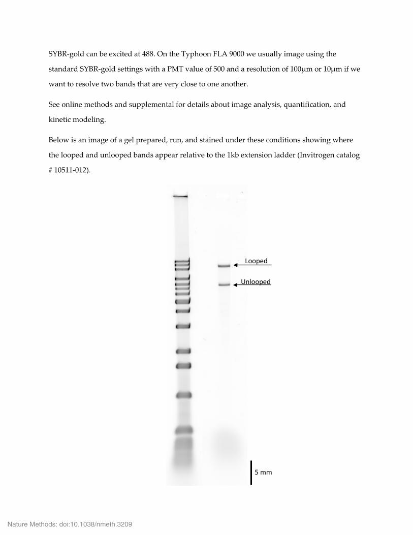
SYBR-gold can be excited at 488. On the Typhoon FLA 9000 we usually image using the

standard SYBR-gold settings with a PMT value of 500 and a resolution of 100μm or 10μm if we

want to resolve two bands that are very close to one another.

See online methods and supplemental for details about image analysis, quantification, and

kinetic modeling.

Below is an image of a gel prepared, run, and stained under these conditions showing where

the looped and unlooped bands appear relative to the 1kb extension ladder (Invitrogen catalog

# 10511-012).

Looped

Unlooped

5 mm


6. Performing Off-rate experiments:

To perform off-rate experiments you must first form loops and allow them to equilibrate. This

can be done by following the steps in the on-rate experiment with the exception of the

quenching steps (4.1-4.3, 4.4.3, and 4.4.6). Simply mix equal volumes of 160 pM construct and

6nM streptavidin, and allow this to form loops for 10 minutes.

To perform the off-rate experiments samples of loops will be allowed to sit in quenching

conditions for different amounts of time with the idea being that if a loop opens it will do so

irreversibly as the now available binding site will quickly be quenched by the large excess of

free floating biotin in solution. To avoid having to run many gels it is easiest to do the longest

time point first so that all the samples can be run on the same gel. For example, if you wanted

your longest time point to be 72 hours you would mix 10 μl of loops with 2 μl of saturated

biotin 72 hours before you planned on running the gel.

An example time series for the biotin streptavidin system would be to take time points over ~5

days at room temperature in the presence of 200 mM salt. Alternatively, for a quicker

experiment time points can be taken over 3 hours at 50°C and 200 mM NaCl.

To form the loops follow the protocols above to generate linear DNA(1), hybridize on the

functionalized and unfunctionalized oligonucleotides(3), dilute the construct (4.1), and dilute

the streptavidin(4.2).

Once you have the required materials (See 1-4.3) You may proceed to do an off-rate experiment:

6.1 Forming loops

6.1.1 ____ Add 70 μl of the 160 pM construct to a new protein LoBind tube

6.1.2 ____ Add 70 μl of the 6nM streptavidin to the 40 μl of DNA

6.1.3 ____ Allow this to sit at 25° C for 10 minutes to allow loop formation to go to

completion


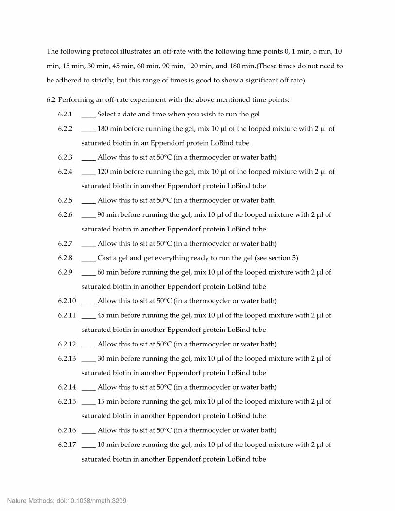
The following protocol illustrates an off-rate with the following time points 0, 1 min, 5 min, 10

min, 15 min, 30 min, 45 min, 60 min, 90 min, 120 min, and 180 min.(These times do not need to

be adhered to strictly, but this range of times is good to show a significant off rate).

6.2 Performing an off-rate experiment with the above mentioned time points:

6.2.1 ____ Select a date and time when you wish to run the gel

6.2.2 ____ 180 min before running the gel, mix 10 μl of the looped mixture with 2 μl of

saturated biotin in an Eppendorf protein LoBind tube

6.2.3 ____ Allow this to sit at 50°C (in a thermocycler or water bath)


saturated biotin in another Eppendorf protein LoBind tube

6.2.5 ____ Allow this to sit at 50°C (in a thermocycler or water bath




6.2.8 ____ Cast a gel and get everything ready to run the gel (see section 5)























6.2.23 ____ 10 μl of an unquenched sample held at the same temperature can be used as

your 0 point

6.2.24 ____ Add 2 μl of 6x ficoll loading dye to each of the samples right before loading and

running the gel

� Some of the liquid may have condensed on the cap. Mild centrifugation can

help ensure that all of your volumes are the same

6.2.25 ____ Load, run, stain, and image the gel as described in section 5

Note: if you wish to do the off-rate in different solution conditions, all you need to do is alter

the buffer in which you dilute your streptavidin and your construct. If you wish to do the off

rate at a different temperature you simply need to let the samples sit in a water bath or

thermocycler set to the desired temperature rather than at room temperature.

See online methods, Halvorsen et. al 2011 and Koussa et. al 2014 for information on how to

implement the nanoswitch platform for non-biotin-streptavidin systems.


nature methods: doi:10.1038/nmeth to 5 topological states indicated by the bold letters a, b, c, d,...

Documents