MPRAMunich Personal RePEc Archive

Natural Selection, Irrationality andMonopolistic Competition

Luo, Guo Ying

McMaster University- DeGroote School of Business

May 2009

Online at http://mpra.ub.uni-muenchen.de/15357/

MPRA Paper No. 15357, posted 21. May 2009 / 16:03

brought to you by COREView metadata, citation and similar papers at core.ac.uk

provided by Research Papers in Economics

Natural Selection, Irrationality and Monopolistic Competition

Guo Ying Luo1

DeGroote School of Business

McMaster University

ABSTRACT

This paper builds an evolutionary model of an industry where firms produce dif-

ferentiated products. Firms have different average cost functions and different demand

functions. Firms are assumed to be totally irrational in the sense that firms enter the

industry regardless of the existence of profits; firms’ outputs are randomly determined

rather than generated from profit maximization problems; and firms exit the industry

if their wealth is negative. It shows that without purposive profit maximization as-

sumption, monopolistic competition still evolves in the long run. The only long run

survivors are those that possess the most efficient technology, face the most favorable

market conditions and produce at their profit maximizing outputs. This paper modifies

and supports the classic argument for the derivation of monopolistic competition.

JEL classification: D21, D43, L10

Keywords: Evolution, Natural Selection, Irrationality, Monopolistic Competition, Sur-

vival of the Fittest

1Correspondent: Guo Ying Luo, Department of Finance and Business Economics, DeGroote Schoolof Business, McMaster University, 1280 Main Street West, Hamilton, Ontario, Canada, L8S 4M4. Tel:(905)525-9140 ext 23983. Email: luogy@mcmaster.ca

1 Introduction

The notion of monopolistic competition was invented in responding to the severe lim-

itation in conducting economic analysis using a framework of either pure competition

or pure monopoly. Monopolistic competition has elements of both pure competition

and pure monopoly. It examines an industry where competing firms produce similar

but different commodities. Due to the product differentiation, each firm has a certain

degree of monopoly power. This is reflected in firms’ downward-slope demand curves.

The free entry and exit condition along with firms’ profit maximization behavior leads

the industry to long-run zero profits. The corresponding firms’ outputs are the ones

that maximize their respective profits. In other words, they produce at the tangency

point where their demand curves are tangent to their respective average cost curves.

Chamberlin (1933) and Robinson (1933) both derive this same equilibrium using differ-

ent techniques. In their derivation of this equilibrium, they both heavily rely on the

rationality and purposive profit maximization behavior on firms’ part.

However, there are a variety of reasons that firms cannot possibly maximize their

profits or profit maximization may not be their objective (see Baumol (1959), Williamson

(1964), Simon (1979), Arrow (1986), Andrews (1949), and Cyert and March (1963)).

Without the purposive profit maximization behavior, could monopolistic competition

still arrives as a long-run equilibrium? Could the classic argument for the derivation of

monopolistic competition still holds?

The early literature (e.g., Alchian (1950), Enke (1951), Friedman (1953)) presents

market selection argument to validate profit maximization hypothesis. Alchian (1950)

writes "Realized positive profits, not maximum profits, are the mark of success and

viability. It does not matter through what process of reasoning or motivation such

2

success was achieved. The fact of its accomplishment is sufficient. This is the criterion

by which the economic system selects survivors: those who realize positive profits are

the survivors; those who suffer losses disappear.". Enke (1951) presents more details

on how the market selection works. Enke (1951) says that "In the long run, however,

if firms are in active competition with one another rather than constituting a number

of isolated monopolies, natural selection will tend to permit the survival of only those

firms that either through good luck or great skill have managed, almost or completely,

to optimize their position and earn the normal profits necessary for survival. In these

instances the economist can make aggregate predictions as if each and every firm knew

how to secure maximum long-run profits.". Friedman (1953) also advocates that "The

process of natural selection thus helps to validate the hypothesis (of profit maximization)

or, rather, given natural selection, acceptance of the hypothesis can be based largely on

the judgment that it summarizes appropriately the conditions for survival."

Later, Winter (1964, 1971), and Nelson and Winter (1982) further examine this

market selection argument in the context of retained earnings dynamics. They found that

the retained earnings of profit maximizers will grow fastest and eventually those firms

will dominate the market. Nelson and Winter (1982) present a partial equilibrium model

where prices are fixed and all firms have access to the same technology; it shows that

"as if " profit maximization describe the long run steady state of firms’ behavior. Dutta

and Radner (1999), and Blume and Easley (2002) examine whether natural selection

favors profit maximizing firms in models with added capital market, where firms can

grow through retained earnings or through financing in the capital markets. Dutta and

Radner (1999) shows that all surviving firms are not profit maximizing firms. Blume and

Easley (2002) shows that the market selection favors profit maximizing firms, but the

3

long-run behavior of evolutionary market models is not well described by the equilibrium

models based on the profit maximization hypothesis.

Luo (1995, 2007) present two evolutionary models of industry dynamics, which sup-

port the profit maximization hypothesis through the market selection arguments. Fur-

thermore, in both papers, the long-run behavior of the industries is consistent with the

one based on the profit maximization hypothesis. The papers basically says that even

though firms are not maximizing their profits (their outputs are randomly determined

upon their entry to the industry), natural selection selects for the firms that happen to

produce at profit maximizing outputs, which in turn promote rational aggregate mar-

ket outcomes. Specifically, Luo (1995) examines an industry where all firms produce a

homogenous commodity. It formally proves that with firms’ total irrationality, perfect

competition as a long run equilibrium evolves with the "as if " profit maximizers as

the only survivors. Luo (2007) obtains similar conclusion in examining a more complex

industry structure where firms produce similar but differentiated products. Namely, the

monopolistic competition arrives as a long run outcome where only the "as if" profit

maximizers survive. Luo (2007) assumes the symmetric demand function and identical

average cost function for all firms. However, this paper builds on these models and

assumes the non-symmetric demand function and non-identical average cost function

for all firms. Specifically, this paper constructs an evolutionary model of an industry

where firms produce similar but differentiated products and each firm has its own in-

herent demand and average cost function. Firms enter the industry sequentially over

time. Each firm’s output is randomly determined upon its entry and fixed thereafter.

If a firm realizes a profit, the profit becomes a part of its wealth. If a firm’s wealth

is positive at the beginning of a period, the firm will continue to produce its product

4

next period; otherwise, the firm exits the industry at the end of that time period. The

nonnegative wealth serves as a market selection criterion. This type of modelling strat-

egy completely rules out firms’ rationality in their decision of entry to the industry, exit

from the industry; and in the determination of the level of their outputs to produce. The

paper concludes that with non-symmetric demand function and non-identical average

cost function, not all "as if " profit maximizers will survive. The firms producing at

their minimum efficient scales will not survive. The only survivors in the long run are

the "as if " profit maximizers who possess the most efficient technology and face the

most favorable market conditions. In aggregate, monopolistic competition arises in the

long run. This paper modifies and supports the classic argument for the derivation of

monopolistic competition. In other words, firms’ rationality is not needed in achieving

monopolistic competition. In addition, the long run survivors produce at a suboptimal

level of output (less than their minimum efficient scales). This is consistent with the

empirical findings in the industrial organization literature (see Weiss (1963 and 1976),

Scherer (1973), and Pratten (1971)) that a majority of firms are not only small but also

small enough so as to operate at a suboptimal level of output (instead of the minimum

efficient scale) in most industries.

2 The Model

Consider an industry where firms enter sequentially over time, producing a similar but

differentiated products. For simplicity, one firm is assumed to enter the industry each

time period. The firm that enters at time period t, where t = 1, 2, ..., is referred to as

firm t. Firm i, where i = 1, 2, ..., produces a level of output αQi, where α is a positive

parameter and it reflects the size of the firm relative to the market and where Qi is

5

randomly taken upon entry period from the interval [Q,Q], 0 < Q < Q < +∞.

The demand function for firm i, i = 1, 2, ..., at time t, t ≥ i, is as follows,

P it (αQ

i) = Ai

⎛⎜⎜⎝1− Xj∈St−1j 6=i

BjαQj

⎞⎟⎟⎠− aiαQi, (1)

where the parameters Ai, Bj, and ai belong to the intervals [A,A], [B,B], and [a, a],

0 <A < A < +∞, 0 < B < B < +∞, and 0 <a < a < +∞, respectively. Ai is firm i’s

price-intercept when all other firms are producing zero output. From hereon, Ai will be

referred to as firm i’s base intercept of its demand curve. St−1 is a set of firms that enter

before time period t and are producing at time period t, excluding firm t. The above

indicates that different firms’ demand curves may have different slopes and different

intercepts, but each firm has the same impact (i.e., Bj is the same for i = 1, 2, ...) on

the intercepts of all other firms’ demand curves.

There is entry cost in the industry. Firm i0s average entry cost is assumed to be

βik, where βi ∈ [β, β], 0 < β < β < +∞, and k > 0. Firm i0s entry cost incurs only

upon entry and there are no longer entry costs for firm i in all subsequent time periods

after its entry.

Firm i’s average cost functions is denoted as Ci(·), Ci(·) is continuous and it has a

negative first derivative and a positive second derivative, i.e., ∂Ci(Qi)∂Qi < 0, ∂2Ci(Qi)

∂Qi2> 0.

Furthermore, for given parameters Q∗ and Q∗, where Q∗ >Q and Q

∗< Q, there exists

a Q∗i ∈ [Q∗, Q∗] such that

∂C i(Q i)

∂Q i|

Q i=Q∗i

= −ai (2)

6

and

Ci(Q∗i ) = c∗i . (3)

The parameters Ai, Bi, ai, Qi, βi, and c∗i are firm i-specific and they are, in the

beginning of firm i’s entry period, randomly and mutually independently taken from

the intervals [A,A], [B,B], [a, a], [Q,Q], [β, β], and [c∗, c∗] according to some given

distributions with full support. In addition, firm i’s average cost function Ci(·) is firm-i

specific. It is also drawn, after the values of ai and c∗i are taken, in the beginning of firm

i’s entry period from U i according to a given distribution with full support, where2

U i = {f(·) : [Q,Q]→ (c,+∞), f(·) is continuous and f 0(·) < 0, f 00(·) > 0;

furthermore, there exists Q∗i ∈ [Q∗, Q∗] such that f(Q∗i ) = c∗i , f

0(Q∗i ) = −ai}

Since the purpose of this paper is to show the convergence of the industry to a mo-

nopolistically competitive equilibrium where the size of each firm is infinitesimally small

relative to the market demand, it is necessary to transform the average cost function of

each firm as a function of the scale parameter (α) while preserving the relevant prop-

erties of the original average cost function. This α− transformation is an effective way

of shrinking the scale of the firm relative to the aggregate market demand. This tech-

nique has been used in papers such as Novshek (1985), Robson (1990), Luo (1995) and

Luo (2007). The shrinking of the scale parameter α towards zero represents increased

competition among firms.

2The reason for conditioning the choice of Ci(·) on the values of ai and c∗i is to ensure that for anygiven demand curve there exists Q∗i ∈ [Q∗, Q

∗] at which a shifted demand curve would eventually be

tangent to firm i’s average cost curve. Otherwise, a random picking of Ci(·) might mean no such tan-gency would occur for Qi ∈ [Q∗, Q∗]. From the perspective of analyzing a monopolistically competitiveequilibrium, this would be uninteresting.

7

The α−transformed average cost function for firm i is defined as Ciα(·) according to

Ciα(Q

i) = Ci(Qi

α) + ai

µQi

α−Q∗i

¶− ai

¡Qi − αQ∗i

¢. (4)

If α = 1, Ciα(·) is the same as Ci(·). This α−transformed average cost function for firm i

generates a family of average cost functions, which shifts towards the Y-axis as α shrinks

towards zero and it preserves the same slope and the same magnitude of the firm i0s

cost function at the output level αQ∗ as α shrinks. Furthermore, firm i0s average cost

at the output level of αQi is above the corresponding point on the tangent line to firm

i0s average cost curve going through the point (αQ∗i , c∗i ). These properties of firm i0s

average cost function are formally stated in Proposition 1.

Proposition 1 (1) For any given α, Ciα(αQ

∗i ) = Ci(Q∗i ) = c∗i for any i = 1, 2, ...

(2) For any given α, ∂Ciα(αQ

i)∂(αQi)

|αQi=αQ∗i

= ∂Ci(Qi)∂Qi |

Qi=Q∗i

= −ai; for any i = 1, 2, ...

(3) Ciα(αQi) ≥ c∗i + aiα(Q∗i −Qi).

Proof. See Appendix A for the proof.

In addition, this α−transformation ensures that firm i0s profit maximizing point Q∗i

remain the same. This is formally stated in the following proposition.

Firm i’s normalized per unit profit at time period t, where t ≥ i ≥ 1, is defined as

Πit(αQ

i) according to

Πit(αQ

i) =

⎧⎪⎨⎪⎩P it (αQ

i)−Ciα(αQ

i)−βikAi , if i = t

P it (αQ

i)−Ciα(αQ

i)

Ai , if i < t.(5)

Then, the following is true.

8

Proposition 2 the normalized per unit profit for firm i that produces at αQ∗i is maxi-

mized, i.e.,

Πit(αQ

i) |Qi=Q∗i

≥ maxQi∈[Q,Q]

Πit(αQ

i). (6)

Proof. See Appendix A for the proof.

Luo (1995) and Luo (2007) presents their models where all firms have the conventional

symmetric demand curves and the same average cost curves. Both papers show that the

ultimate surviving firms are those that act as if they were profit maximizers. Obviously,

in this more general setting where firms have different demand curves and different

average cost curves, some firms have more technological advantage or face better market

conditions. Interesting questions to be asked are whether the long run survivors are still

those that happen to produce at their profit maximizing outputs; and, whether more

efficient technologies and better market conditions play any role in determining the long

run survivors.

The following proposition shows that each time period with a strictly positive proba-

bility (however small) firms enter with the most efficient technology and facing the best

market conditions along with producing at their profit maximizing outputs.

Proposition 3 For any given > 0, there exists a θ ∈ [0, 1] , such that for i = 1, 2, ...,

Pr³Ciα(αQ

i) ∈ [c∗i , c∗i + ], Ciα(αQ

i)Ai

∈ [ c∗A, c∗

A+

A]´= θ > 0.

Proof. See appendix A for the proof.

Remark: Essentially, Proposition 3 says that in each time period, there is a strictly

positive probability that a firm enters, producing at the tangency of its average cost

curve to its demand curve, having the most efficient technology and facing the best

market conditions. In fact, those firms resemble the profit maximizing firms and have

9

the ratio of its profit maximizing average cost to the base intercept of its demand curve

being the smallest among all firms producing at tangency points.

A firm’s wealth at the end of a time period is defined as an accumulative profits up to

the end of that time period. If a firm’s wealth at the end of one time period is negative,

then this firm must exit the industry at the end of that time period. Otherwise, this firm

will continue to produce in the next time period. This assumption serves as a market

selection criterion. The detail dynamics of the industry is described in the following.

For simplicity, it is assumed that there is no firm in the industry at the initial time

period. At the beginning of time period 1, only one firm (called firm 1) enters the

industry, producing αQ1 of product 1. The price of product 1 at time 1 is P 11 (αQ

1) =

A1(1 −Pi∈S0(BiαQi)) − a1αQ1, where S0 is a set of firms that have entered before time

period 1 and are producing in time period 1. By the assumption, S0 = φ. Hence, the

price for product 1 of firm 1 is P 11 (αQ

1) = A1 − a1αQ1. Firm 1’s total entry cost is

β1kαQ1 and its average cost is Cα(αQ1). It follows that firm 1’s profit at time 1 is

(P 11 (αQ

1)−Cα(αQ1)− β1k)αQ1. Firm 1’s wealth at the end of time period 1 is defined

as W 11 = (P

11 (αQ

1)−Cα(αQ1)− β1k)αQ1. Firm 1 continues to produce αQ1 of product

1 at time 2 if W 11 ≥ 0 and otherwise exits the industry at the end of time 1.

At the beginning of time period 2, another firm (labeled as firm 2) enters the industry,

producing αQ2 of product 2. The price for product 2 at time 2 is P 22 (αQ

2) = A2(1 −Pi∈S1(BiαQi)) − a2αQ2, where S1 is a set of firms, which entered in time period 1 and

are continuing to produce at time 2. Specifically, S1 = {1 :W 11 ≥ 0} ∪ φ. Firm 2’s total

entry cost is β2kαQ2 and its average cost is Cα(αQ2); hence, firm 2’s profit at time 2 is

(P 22 (αQ

2)−Cα(αQ2)− β2k)αQ2. Firm 2’s wealth at the end of time period 2 is defined

as W 22 = (P

22 (αQ

2)−Cα(αQ2)− β2k)αQ2. Firm 2 continues to produce αQ2 of product

10

2 at time 3 if W 22 ≥ 0 and otherwise exits at the end of its entry period 2.

If firm 1 is producing αQ1 of product 1 at time 2 (i.e., firm 1 has had a nonnegative

wealth at time 1), then firm 1 has survived period 1 and continues producing αQ1

of product 1 in the industry in time period 2. Firm 1’s product price at time 2 is

P 12 (αQ

1) = A1(1−P

i∈S1∪{2},i6=1(BiαQi))− a1αQ1. Note that the entry firm (i.e., firm 2)

is included from the intercept of firm 1’s demand function at time period 2. If firm 1’s

wealth is nonnegative at the end of time period 1, then firm 1’s wealth at the end of time

period 2 is defined as an accumulative profits up to the end of time period 2. That is,

W 12 = W 1

1+ (P12 (αQ

1) − Cα(αQ1))αQ1. Furthermore, firm 1 continues to produce αQ1

of product 1 at time 3 if firm 1’s wealth is nonnegative at time 2 (i.e., W 12 ≥ 0) and

otherwise, firm 1 exits at the end of time period 2.

This process goes on and on. In general, at the beginning of time t, one firm (labeled

as firm t) enters the industry, producing αQt of product t. The price of product t at time

t is P tt (αQ

t) = At(1−P

i∈St−1(BiαQi))−atαQt, where St−1 is a set of firms, which entered

before and in time period t− 1 and are still producing at time t, i.e., St−1 = {i ≤ t− 1 :

W ii ≥ 0, W i

t0 ≥ 0 for all t0 ∈ (i, t− 1]} ∪ φ, where W ii = (P

ii (αQ

i)− Cα(αQi)− βik)αQi

and W it0 =W i

t0−1+(Pit0−1(αQ

i)−Cα(αQi))αQi for all t0 ∈ (i, t− 1]. In other words, St−1

is a set of firms that have survived all time periods up to the end of time period t− 1

and remain in the market at time t. Firm t’s total entry cost is βtkαQt and its average

cost is Cα(αQt); hence, firm t’s profit at time t is (P t

t (αQt)−Cα(αQ

t)− βtk)αQt. Firm

t0s wealth is W tt = (P

tt (αQ

t)−Cα(αQt)− βtk)αQt. Firm t continues to produce αQt of

product t at time t + 1, if firm t’s wealth is nonnegative and otherwise firm t exits at

the end of time period t.

If firm i, where i < t, has nonnegative wealth in all time periods before time t, (i.e.,

11

W ii ≥ 0, W i

t0 ≥ 0 for all t0 ∈ (i, t−1]), then firm i has survived all time periods up to the

end of time t− 1 and remains producing αQi of product i in the industry in time period

t. Firm i’s product price at time t is P it (αQ

i) = Ai(1−P

j∈St−1∪{t},j 6=i(BjαQj))− aiαQi.

Note that the entry firm (i.e., firm t) is included from the intercept of firm i’s demand

function at time period t. If firm i’s wealth is nonnegative at the end of time period

t − 1, then firm i’s wealth at the end of time period t is defined as an accumulative

profits up to the end of time period t. That is, W it =W i

t−1+ (Pit (αQ

i)− Cα(αQi))αQi.

Furthermore, firm i continues to produce αQi of product i at time t+1 if firm i0s wealth

is nonnegative at time t (i.e., W it ≥ 0) and otherwise, firm i exits at the end of time

period t.

To ensure that all firms producing at arbitrarily close to their profit maximizing

outputs can potentially make positive profits upon their entry periods, it is assumed

that Ai > c∗i +βik for i = 1, 2, .... Otherwise, no such firm can make positive profit upon

its entry period and consequently no such firm can survive in the industry for more than

one period.

3 The Results

Under the firm-specific cost curves and the firm-specific demand curves, the following

theorem shows that as the size of each firm becomes infinitesimally small relative to the

market, as the entry cost becomes sufficiently small, and as time gets sufficiently large,

the industry converges in probability to the monopolistically competitive equilibrium,

where the only surviving firms are those producing at outputs on their average cost

curves tangent to their demand curves, and furthermore at these outputs the ratios of

their average costs to the base intercepts of their demand curves are the smallest among

12

all firms producing at tangency outputs. Firms that have such smallest ratios are those

having the most efficient technologies and facing the best market conditions. The results

are precisely stated in the following theorem.

Theorem 1 For any given positive numbers and η ∈ (0, 1), there exist positive num-

bers α and k such that, for any α < α and for 2Aβ(2A+A)

< k < k, there exists a time

period τ( , η, α, k) such that, for all t > τ( , η, α, k),

(i(a))

Pr

⎛⎜⎝ c∗Ai

A+ aiα (Qi

∗ −Qi) < P it (αQ

i) < c∗Ai

A+ aiα (Q∗i −Qi) + ,

for all i ∈ {t} ∪ St

⎞⎟⎠ > 1− η;

(i(b))

Pr

⎛⎜⎝ c∗i + aiα (Q∗i −Qi) < P it (αQ

i) < c∗i + aiα (Q∗i −Qi) + ,

for i ∈ {t} ∪ St ∩½i0 :

c∗i0

Ai0∈∙c∗

A,c∗

A+2A+A

¸¾.

⎞⎟⎠ > 1− η;

(ii) with probability of at least 1− η, each of the remaining firms, say firm i, is the

one withc∗iAi∈∙c∗

A,c∗

A+

A

¸and having the average costs lying in the interval

[c∗i + aiα (Q∗i −Qi) , c∗i + aiα (Q∗i −Qi) + ) , i.e.,

Pr

⎛⎜⎝ c∗i + aiα (Q∗i −Qi) ≤ Ciα(αQ

i) < c∗i + aiα (Q∗i −Qi) +

andc∗iAi∈∙c∗

A,c∗

A+

A

¸, for all i ∈ St

⎞⎟⎠ > 1− η;

(iii) with probability of at least 1−η, no new entrant firm, say firm t, with the average

cost lying outside the interval [c∗t + atα (Q∗t −Qt) , c∗t + atα (Q∗t −Qt) + ) or satisfyingc∗tAt

/∈∙c∗

A,c∗

A+

A

¸can make positive profit by entry. That is, for firm t, producing αQt,

13

where Ctα(αQ

t) /∈ [c∗t + atα (Q∗t −Qt) , c∗t + atα (Q∗t −Qt) + ) orc∗tAt

/∈∙c∗

A,c∗

A+

A

¸,

Pr¡P tt (αQ

t)− Ctα(αQ

t)− βtk < 0¢> 1− η.

Proof. See Appendix B for the proof.

Remark: Shrinking the α and k represents ways of shrinking the scale of firms relative to

the market and shrinking entry costs to zero, respectively. As the α and k get smaller,

the industry eventually comes closer to monopolistic competition as time goes by. In

the limit, monopolistic competition evolves as a long run outcome of the industry where

firms are producing at the tangency of their average cost curves to their respective

demand curves, where firms are infinitesimally small relative to the market and where

there is no entry barrier. The technical characterizations of the long run equilibrium

outcomes are provided in Theorem 1. According to Part (ib), prices of all producing firms

are arbitrarily close to c∗i where their average cost curves is tangent to their respective

demand curves. Notice from part (ia)that the prices for some firms could be below

their average costs (due to c∗Ai

A< c∗i ). Nevertheless, part (ii) indicates that such firms

would not survive in the long run. According to part (ii), the only surviving firms

are those producing at arbitrarily close to the tangency of their average cost curves

to their respective demand curves (i.e., resembling profit maximizing firms), and using

a technology arbitrarily close to the most efficient technology (with c∗) and serving a

market arbitrarily close to the largest market (with A) (i.e., facing the best market

conditions). Furthermore, part (iii) indicates that no new entrant firms not producing

at arbitrarily close to the tangency output or not having the most efficient technology

or not facing the best market conditions, could enter and make positive profits. In

addition, it is worth mentioning that in the process of shrinking the α and k, the k

14

must be maintained to be sufficiently high relative to the scale of parameter α. This is

reflected in the lower bound, 2Aβ(2A+A)

, for the k. Otherwise, the entry cost loses its role

of creating entry barriers to the industry.

Furthermore, the results in Theorem 1 suggest that the long run survivors are pro-

ducing at a suboptimal scale of their outputs in the sense that their output levels are

less than their minimum efficient scales. This is consistent with the well documented

empirical findings in the industrial organization literature (see Weiss (1963 and 1976),

Scherer (1973), and Pratten (1971)) that a majority of firms are not only small but

also sufficiently small so as to operate at a suboptimal scale of output (instead of the

minimum efficient scale) in most industries.

4 Conclusion

This paper builds a dynamic model of an industry where firms produce similar but

differentiated products. Firms have different entry costs and average cost functions as

well. Firms face different demand functions.

Conventionally, to achieve monopolistic competition, the key driving force is that

firms are assumed to maximize profits in their entry decision, in selecting output level

and in their decision of when to exit the industry (see Chamberlin (1933) and Robinson

(1933)). However, due to the recent criticism on firms’ rationality, this paper attempts

to explain monopolistic competition without purposive profit maximization assumption.

This is achieved by applying an evolutionary idea of natural selection to the industry

competition. Firms enter the industry regardless of the existence of profits; firms’ out-

puts are randomly determined rather than generated from profit maximization problems;

and firms exit the industry if their wealth is negative.

15

A group of papers in this literature provide positive support to the hypothesis of the

"as if" profit maximizers as long run survivors through market selection argument. This

paper shows that not all of these firms will survive in this general setting of industry.

The only long run survivors are those that possess the most efficient technology, face

the most favorable market conditions and produce at their profit maximizing outputs.

Moreover, at the aggregate level, monopolistic competition arises in the long run. This

paper modifies and supports the classic argument for the derivation of monopolistic

competition. In addition, the results in this paper is consistent with the common

observation in the industrial organization that a majority of the firms are not only small

but also sufficiently small so as to operate at suboptimal scale of output (instead of the

minimum efficient scale) in most industries.

16

Appendix A

Proof of Proposition 1: (1) The result can be obtained by replacing Qi with αQ∗i in

equation (4) and then applying equation (3) to the resulting equation.

(2) Rewrite equation (4) into the following:

Ciα(αQ

i) = Ci(Qi) + ai¡Qi −Q∗i

¢− ai

¡αQi − αQ∗i

¢then taking a derivative of the above equation and then applying equation (2 ) results

in the following equation:

∂C iα(αQ

i)

∂(αQ i)|

αQi=αQ∗i

=∂C i(Q i)

∂Q i|

Q i=Q∗i

= −a i .

(3) Since Ciα(αQ

∗i ) = c∗i for any i = 1, 2, ..., ∂Ci

α(αQi)

∂(αQi)|

αQi=αQ∗i

= −ai; and ∂2Ciα(αQ

i)∂(αQi)2

>

0, the result follows.¥

Proof of Proposition 2: Substitute equations (1) and (4) into equation (5). Then use

the resulting equation and take the first order and the second order of firm i0s normalized

per unit of profit with respect to Qi. Finally apply property (2) of Proposition 2 along

with the assumption of ∂2Ciα(αQ

i)∂(αQi)2

> 0 to obtain equation (6).¥

Proof of Proposition 3: Since, conditional on ai and c∗i , the random draws of Qi

and the continuous average cost function Ci(·) are mutually independent, it follows that

Ci(αQi) has a strictly positive probability of taking a value in the interval [c∗i , c∗i + ],

where is any given small positive number. It is also true that Ci(αQi) has a strictly

positive support at c∗. Finally, since Ai has a strictly positive support at A, and given

the fact that Ai is independent of all the random variables ai, c∗i , Qi, and Ci(·) and given

17

the α−transformation of the average cost function, it follows that with a strictly positive

probability,

Pr

µCiα(αQ

i) ∈ [c∗i , c∗i + ],Ciα(αQ

i)

Ai∈ [c

∗

A,c∗

A+

A]

¶> 0.

Furthermore, given that the sequences {ai}i≥1 , {c∗i }i≥1 , {Qi}i≥1 and {Ci(·)}i≥1 are

independently and identically distributed, respectively; since Qi is independent of aj, c∗j

and Cj(·) for i, j = 1, 2, ...; the ai is independent of c∗j for all i and j; and the Ci(·) is

independent of aj and c∗j for i 6= j, it follows that there must exists a θ ∈ (0, 1) , such

that for i = 1, 2, ...,Pr³Ciα(αQ

i) ∈ [c∗i , c∗i + ], Ciα(αQ

i)Ai

∈ [ c∗A, c∗

A+

A]´= θ.¥

Appendix B

Theorem 1 is directly established by using the results in two lemmas, namely, Lemma

1 and Lemma 2. Lemmas 1 and 2 are first proven.

For the purpose of simplifying the proof, denote qi = aiQi for any i, q∗i = aiQ∗i for any

i, and bj = Bj

ajfor any j and furthermore, define q = aQ, q = aQ, q∗ =a Q∗, q∗ = aQ

∗,

b= Baand b = B

a. Therefore, firm i0s demand function can be expressed, in terms of qi,

as follows:

P it (αQ

i) = P it (α

qi

ai) = Ai

⎛⎜⎜⎝1− Xj∈St−1j 6=i

bjαqj

⎞⎟⎟⎠− αqi,

where qi ∈ [q, q] and bj ∈ [b, b]. Similarly, firm i0s average cost function can also be

expressed, in terms of qi, as

Ciα(αQ

i) = Ciα(αqi

ai) = Ci(

qi

ai) +

¡qi − q∗i

¢− α

¡qi − q∗i

¢.

18

Define pit(αqi) = P i

t (αqi

ai) and define ciα(αq

i) = Ciα(

αqi

ai). Notice that for the above

transformation, ciα(αqi) =Ci

α(αQi); therefore, ciα(αq

∗i ) = Ci

α(αQ∗i ) = Ci(Q∗i ) = c∗i .

pit(αqi) = P i

t (αQi). In addition, for any given α,

∂ciα(αqi)

∂(αqi)|

αqi=αq∗i

=∂pit(αq

i)

∂(αqi)= −1,

for any i = 1, 2, ... This means that the slope of a firm’s tangent line to its average cost

function at the output level of αq∗i is the same across all firms.

Furthermore, normalize the following variables by Ai. That is, define, for i = 1, 2, ...,

epit(αqi) = pit(αqi)

Ai, eciα(αqi) = ciα(αq

i)

Ai, eqi = qi

Ai, eq∗i = q∗i

Ai, ec∗i = c∗i

Ai, eβi = βi

Ai. Denote

ec∗ = c∗

A, eq∗ = q∗

A,eq∗ = q∗

A, eβ = β

Aand eβ = β

A. Hence, each firm’s demand function in

terms of epit(αqi) has the same base intercept.For t = 1, 2, ..., define Itt as the following:

Itt =

⎧⎪⎨⎪⎩ 1 if ptt(αqt) ≥ ctα(αq

t) + βtk

0 otherwise

If Itt = 1, then firm t makes a nonnegative profit on the entry period.

Lemma 1 establishes a lower bound for firms’ prices after shrinking firms’ size relative

to the market (i.e., α). The lower bounds are arbitrarily close to c∗ ( which is the

tangency of the most efficient firms’ average cost curves to their respective demand

curves).

Denote St = {t} ∪ St−1 for t = 1, 2, ....

Lemma 1 For any given k, for any given positive 0 <Aβk

2, there exists an α such that,

for α < α, at any time period t, where t = 1, 2, ..., for i ∈ St,

epit(αqi) > ec∗ + α¡eqi∗ − eqi¢+ 0

A.

19

Proof. Define ebP t =

Ã1−

Xi∈St

bi(αqi)

!, for t = 1, 2, ... (7)

Lemma 1 first proves the following claim.

Claim: For any given k, and for any given positive 0 <Aβk

2, there exists an α1 such

that for α < α1,ebP t ≥ ec∗ + αeq∗ + eβk − 0

A, for all t = 1, 2, ....

Proof of Claim: This is shown by induction.

(1) The base step of the induction proof: The claim is true for t = 1. For any given

k, and for any given positive 0 <Aβk

2, define α1 such that

−bα1q = α1eq∗ − 0

A, or α1 =

0

A¡bq + eq∗¢ . (8)

Since ebP 1 = (1− b1αq1I11 ). This together with equation (8) and q1 ≤ q and A1 > c∗1+β1k

implies that ebP 1 ≥ 1− bαq > ec∗1 + αeq∗ + eβ1k − 0

A> ec∗ + αeq∗ + eβk − 0

A, for α < α1.

(2) The induction step: Suppose that the claim is true for t = r, i.e., for any given

k, and for any given positive 0 <Aβk

2, there exists an α1 such that for α < α1, at time

period r, ebP r ≥ ec∗ + αeq∗ + eβk − 0

A. (9)

It is now shown that the claim is true for t = r + 1, i.e., for the given k, for the given

0 <Aβk

2, if α < α1, then at time period r + 1,

ebP r+1 ≥ ec∗ + αeq∗ + eβk − 0

A. (10)

20

Using equation (7),

ebP r+1 =ebP r − br+1αqr+1Ir+1r+1 +

Xi∈Xr+1i6=r+1

bi¡αqi¢, (11)

where Xr+1 represents a set of firms that exit the industry at the end of time period

r + 1. Equation (11) further implies that

ebP r+1 ≥ ebP r − br+1αqr+1Ir+1r+1 . (12)

Consider the following two cases:

Case 1: Suppose that ebP r− br+1αqr+1Ir+1r+1 −αeqr+1 ≥ ec∗r+1+α¡eq∗r+1 − eqr+1¢+ eβk− 0

A.

Then, using the fact that ec∗r+1 ≥ ec∗, and eq∗r+1 ≥ eq∗, equation (12) implies thatebP r+1 ≥ ec∗ + αeq∗ + eβk − 0

A.

That is, equation (10) holds.

Case 2: Suppose that

ebP r − br+1αqr+1Ir+1r+1 − αeqr+1 < ec∗r+1 + α¡eq∗r+1 − eqr+1¢+ eβk − 0

A. (13)

Notice that

pr+1r+1(αqr+1)

Ar+1= epr+1r+1(αq

r+1) =

Ã1−

Xi∈Sr

bi(αqi)

!− αeqr+1. (14)

21

Using the definition of ebP r (see equation (7)),

ebP r − br+1αqr+1Ir+1r+1 − αeqr+1 = Ã1−Xi∈Sr

bi(αqi)

!− br+1αqr+1Ir+1r+1 − αeqr+1. (15)

Equations (14) and (15) imply that

pr+1r+1(αqr+1)

Ar+1−µebP r − br+1αqr+1Ir+1r+1 − αeqr+1¶ = br+1αqr+1Ir+1r+1 < bαq. (16)

Since, using the definition of α1 in equation (8), bα1q =bqeq∗ + bq

µ 0

A

¶<

0

A, it follows

that for any α < α1,

bαq <0

A.

This together with equation (16) further implies that for α < α1,

pr+1r+1(αqr+1)

Ar+1<ebP r − br+1αqr+1Ir+1r+1 − αeqr+1 + 0

A. (17)

Using equations (13) and (17), it follows that for α < α1,

pr+1r+1(αqr+1)

Ar+1< ec∗r+1 + α

¡eq∗r+1 − eqr+1¢+ eβk. (18)

Since properties (3) of the α-transformed cost function outlined in Proposition 1 in

Appendix A imply that any price for producing αQr+1 on the demand curve which is

tangent to the average cost curve at αQ∗r+1 is no higher than Cr+1α (αQr+1), equation

22

(18), together with Ar+1eβ ≤ βr+1, implies that

pr+1r+1(αqr+1) < c∗r+1 + α

¡q∗r+1 − qr+1

¢+ βr+1k

≤ cr+1α (αqr+1) + βr+1k.(19)

Equation (19) further implies that firm r+1 makes a negative profit in its entry period.

Therefore, firm r+1 must exit the industry at the end of its entry period r+1. That is,

Ir+1r+1 = 0.

Using equation (12), this in turn implies that

ebP r+1 ≥ ebP r,

which together with equation (9) further implies that for any α < α1,

ebP r+1 ≥ ec∗ + αeq∗ + eβk − 0

A.

Therefore, the claim holds.

Now, at time period t = 1, 2, ..., for any firm i ∈ St = {t} ∪ St−1,

pit(αqi)

Ai=ebP t−1 − α

¡eqi − biqi¢− btαqt.

23

This together with the result of the claim and with qt ≤ q implies that for any α < α1,

pit(αqi)

Ai≥ ec∗ + αeq∗ + eβk − 0

A− α (eqi − biqi)− btαqt

= ec∗ + α (eq∗i − eqi) + α¡eq∗ − eq∗i ¢+ eβk − 0

A+ αbiqi − btαqt

> ec∗ + α (eq∗i − eqi) + eβk − 0

A− bαq − αeq∗.

(20)

Then, with 0 <Aβk

2, there exists an α < α1 such that for α < α,

eβk − 0

A−³bαq + αeq∗´ >

0

A. (21)

Therefore, the result of Lemma 1 follows from equation (20) and (21).¥

Lemma 2 establishes a probabilistic upper bound for firms’ prices after a certain time

period for a sufficiently small α. The upper bounds are arbitrarily close to the average

cost plus average entry cost of the firms producing at the tangency of their average cost

curves to their respective demand curves, possessing the most efficient technology, and

facing the best market conditions. The driving force of this result is the allowance for the

entry of firms producing at the tangency of their average cost curves to their respective

demand curves, with the most efficient technology (i.e., c∗) and facing the best market

conditions (i.e., A ). In other words, it is indirectly assumed that each time period with

a positive probability (however small) firms enter the industry with the most efficient

technology (i.e., c∗) and facing the best market conditions (i.e., A ). These firms are

referred to as M-firms in the proof of Lemma 2. The proof of Lemma 2 is done by way of

contradiction. It roughly says that the prices cannot be above the upper bounds after a

certain time period for a sufficiently small α. If they do, then there will be a sufficiently

large number of M-firms entering the industry over the time periods where the prices

24

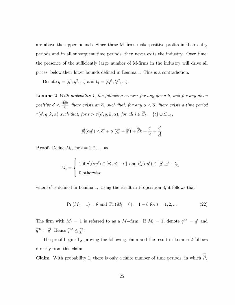
are above the upper bounds. Since these M-firms make positive profits in their entry

periods and in all subsequent time periods, they never exits the industry. Over time,

the presence of the sufficiently large number of M-firms in the industry will drive all

prices below their lower bounds defined in Lemma 1. This is a contradiction.

Denote q = (q1, q2, ...) and Q = (Q1, Q2, ...).

Lemma 2 With probability 1, the following occurs: for any given k, and for any given

positive 0 <Aβk

2, there exists an α, such that, for any α < α, there exists a time period

τ( 0, q, k, α) such that, for t > τ( 0, q, k, α), for all i ∈ St = {t} ∪ St−1,

epit(αqi) < ec∗ + α¡eq∗i − eqi¢+ eβk + 0

A+

0

A

Proof. Define Mt, for t = 1, 2, ..., as

Mt =

⎧⎪⎨⎪⎩ 1 if ctα(αqt) ∈ [c∗t , c∗t + 0] and ectα(αqt) ∈ £ec∗,ec∗ + 0

A

¤0 otherwise

where 0 is defined in Lemma 1. Using the result in Proposition 3, it follows that

Pr (Mt = 1) = θ and Pr (Mt = 0) = 1− θ for t = 1, 2, ... (22)

The firm with Mt = 1 is referred to as a M−firm. If Mt = 1, denote qM = qt and

eqM = eqt. Hence eqM ≤ eq∗.The proof begins by proving the following claim and the result in Lemma 2 follows

directly from this claim.

Claim: With probability 1, there is only a finite number of time periods, in which ebP t

25

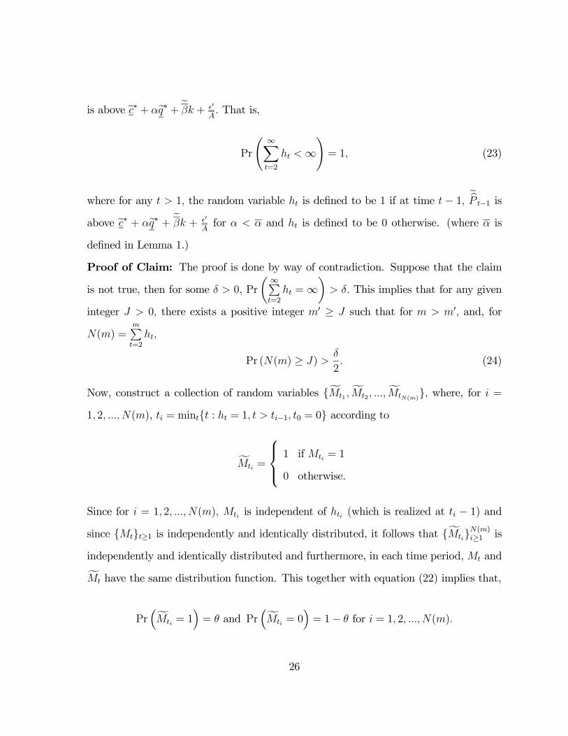
is above ec∗ + αeq∗ + eβk + 0

A. That is,

Pr

à ∞Xt=2

ht <∞!= 1, (23)

where for any t > 1, the random variable ht is defined to be 1 if at time t − 1, ebP t−1 is

above ec∗ + αeq∗ + eβk + 0

Afor α < α and ht is defined to be 0 otherwise. (where α is

defined in Lemma 1.)

Proof of Claim: The proof is done by way of contradiction. Suppose that the claim

is not true, then for some δ > 0, Prµ ∞Pt=2

ht =∞¶> δ. This implies that for any given

integer J > 0, there exists a positive integer m0 ≥ J such that for m > m0, and, for

N(m) =mPt=2

ht,

Pr (N(m) ≥ J) >δ

2. (24)

Now, construct a collection of random variables {fMt1 ,fMt2 , ...,fMtN(m)}, where, for i =

1, 2, ..., N(m), ti = mint{t : ht = 1, t > ti−1, t0 = 0} according to

fMti =

⎧⎪⎨⎪⎩ 1 if Mti = 1

0 otherwise.

Since for i = 1, 2, ..., N(m), Mti is independent of hti (which is realized at ti − 1) and

since {Mt}t≥1 is independently and identically distributed, it follows that {fMti}N(m)i≥1 is

independently and identically distributed and furthermore, in each time period, Mt andfMt have the same distribution function. This together with equation (22) implies that,

Pr³fMti = 1

´= θ and Pr

³fMti = 0´= 1− θ for i = 1, 2, ..., N(m).

26

Since E(fMti) = θ, V ar(fMti) = θ(1− θ) and since θ ∈ (0, 1), it follows that

V ar

⎛⎝N(m)Xi=1

fMti

⎞⎠ < E

⎛⎝N(m)Xi=1

fMti

⎞⎠ . (25)

Denote ZN(m) = E

ÃN(m)Pi=1

fMti

!. Using Chebyshev’s inequality, for any given positive

integer x < ZN(m),

Pr

ÃN(m)Pi=1

fMti ≤ x

!≤ Pr

ï̄̄̄¯N(m)Pi=1

fMti − ZN(m)

¯̄̄̄¯ ≥ ZN(m) − x

!

≤V ar

N(m)

i=1Mti

(ZN(m)−x)2

<ZN(m)

(ZN(m)−x)2 (using equation (25))

This together with the fact that Pr

ÃN(m)Pi=1

fMti ≤ x

!= 1 − Pr

ÃN(m)Pi=1

fMti > x

!implies

that

Pr

⎛⎝N(m)Xi=1

fMti > x

⎞⎠ > 1− ZN(m)¡ZN(m) − x

¢2 .Notice that as N(m) → ∞, ZN(m) → ∞ and

ZN(m)

(ZN(m)−x)2 → 0. Hence, for any given

positive integer x and for any given positive y < 1, there exists a positive integer N,

such that for N(m) ≥ N,

Pr

⎛⎝N(m)Xi=1

fMti > x

⎞⎠ > 1− y > 0. (26)

Define m, such that N(m) = N. SinceN(m)Pi=1

Mti =N(m)Pi=1

fMti, using equation (26), it

27

follows that for m > m,

Pr

⎛⎝N(m)Xi=1

Mti > x |N(m) = r

⎞⎠ > 1− y, for r ≥ N. (27)

Using Proposition 4 in Appendix C, equation (27) also implies that

Pr

⎛⎝N(m)Xi=1

Mti > x¯̄N(m) ≥ N

⎞⎠ > 1− y > 0. (28)

Set J = N in equation (24). Equation (24) means that for this given N, there exists a

positive m0 ≥ N, such that for m > m0,

Pr¡N(m) ≥ N

¢>

δ

2. (29)

Since for m > max(m0,m),

Pr

ÃN(m)Pi=1

Mti > x

!≥ Pr

ÃN(m)Pi=1

Mti > x,N(m) ≥ N

!

= Pr

ÃN(m)Pi=1

Mti > x¯̄N(m) ≥ N

!Pr¡N(m) ≥ N

¢> (1− y) δ

2, (using equations (28)and (29) ).

The above means that for any given positive integer x and for any given positive y < 1,

there exists an integer m0 = max(m0,m) such that for m > m0,

Pr

⎛⎝N(m)Xi=1

Mti > x

⎞⎠ > (1− y)δ

2> 0.

28

This further implies that

Pr

à ∞Xi=1

Mti =∞!

> 0. (30)

This means that with a strictly positive probability the number of M-firms goes to

infinity.

Now, if Mti = 1, then the firm that enters at time ti, where hti = 1, is a M-firm.

Consider this M-firm. When hti = 1, this implies that at time ti − 1, ebP ti−1 is aboveec∗+αeq∗+eβk+ 0

A. This, together with the property that for aM-firm ec∗+ 0

A> ecMα (αqM),eqM ≤ eq∗, implies that

eptiti(αqti) |qti=qM0

=ebP t−1 − αeqM> ec∗ + α

¡eq∗ − eqM¢+ eβk + 0

A

> ecMα (αqM) + eβMk.

This further implies that ptiti(αqM) > ctiα(αq

M)+βtik. This means that thisM-firm’s per

unit revenue at its entry period ( which is ptiti(αqM)) exceeds its per unit cost at its entry

period (which is ctiα(αqM) + βtik). Hence, this M-firm makes a strictly positive profit in

its entry time period and it continues to produce in time period ti+1. Lemma 1 implies

that for this k and 0 and for any α < α, thisM-firm in any subsequent time periods has

its product price greater than per unit cost (which is no more than c∗+ 0) . In other

words, this M-firm makes a strictly positive profit in any subsequent time period after

its entry. Therefore, this M-firm never exits the economy. Equation (30) implies that

with a strictly positive probability there is an infinite number of such M-firms in the

economy. Since thoseM-firms never exit the economy and since each individualM-firm

produces at least αQ , the presence of the infinite number of such M-firms would drive

29

the price for each of the producing firms, say firm i, belowc∗Ai

A+ aiα (Q∗i −Qi) + 0

with a strictly positive probability. This contradicts the result in Lemma 1. Therefore,

equation (23) follows.

Since epit(αqi) = ebP t−1 − αeqi + biαqi − btαqt and since from the proof of Lemma 1,

biαqi ≤ bαq ≤ 0

A, equation (23) further implies that with probability 1 the following

occurs: for this k and 0 <Aβk

2and for any α < α, there must exist a time period, say

τ( 0, q, k, α), such that for all t > τ( 0, q, k, α), for all firms i ∈ St = {t} ∪ St−1,

epit(αqi) ≤ ec∗ + αeq∗ + eβk + 0

A− αeqi + biαqi − btαqt

< ec∗ + α¡eq∗ − eqi¢+ eβk + 0

A+

0

A

≤ ec∗ + α (eq∗i − eqi) + eβk + 0

A+

0

A.

Therefore, Lemma 2 is proven.¥

The results in Theorem are directly established by bringing together the results in

Lemma 1 and 2 along with shrinking of the average entry cost k.

Proof of Theorem 1: (i(a)) Using Lemma 1 and Lemma 2, it follows that with

probability 1, the following occurs: for any given k, for any given positive 0 <Aβk

2,

there exists an α such that, for α < α, there exists a time period τ( , Q, α, k) such that

for t > τ( 0, Q, α, k),

c∗Ai

A+ aiα (Q∗i −Qi) + 0 < P i

t (αQi) < c∗A

i

A+ aiα (Q∗i −Qi) + βA

Ak + 0 + A

A0,

for all i ∈ St = {t} ∪ St−1.

Define k =A

βA0 and = 0

³2 + A

A

´. Then, it follows that with probability 1, the

following occurs: for any given positive , there exist positive numbers k and α such

30

that, for 2Aβ(2A+A)

< k < k and for α < α, there exists a time period τ( , Q, α, k) such

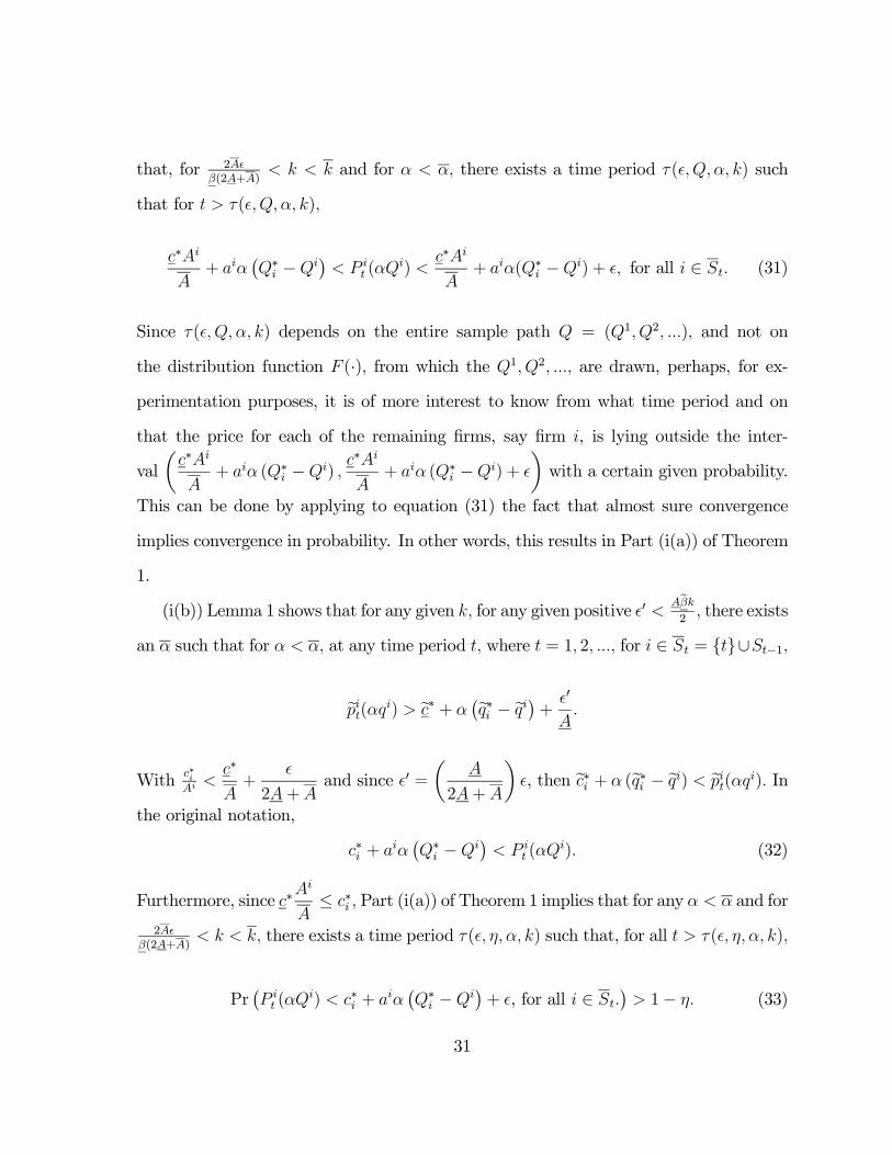
that for t > τ( , Q, α, k),

c∗Ai

A+ aiα

¡Q∗i −Qi

¢< P i

t (αQi) <

c∗Ai

A+ aiα(Q∗i −Qi) + , for all i ∈ St. (31)

Since τ( , Q, α, k) depends on the entire sample path Q = (Q1, Q2, ...), and not on

the distribution function F (·), from which the Q1, Q2, ..., are drawn, perhaps, for ex-

perimentation purposes, it is of more interest to know from what time period and on

that the price for each of the remaining firms, say firm i, is lying outside the inter-

valµc∗Ai

A+ aiα (Q∗i −Qi) ,

c∗Ai

A+ aiα (Q∗i −Qi) +

¶with a certain given probability.

This can be done by applying to equation (31) the fact that almost sure convergence

implies convergence in probability. In other words, this results in Part (i(a)) of Theorem

1.

(i(b)) Lemma 1 shows that for any given k, for any given positive 0 <Aβk

2, there exists

an α such that for α < α, at any time period t, where t = 1, 2, ..., for i ∈ St = {t}∪St−1,

epit(αqi) > ec∗ + α¡eq∗i − eqi¢+ 0

A.

With c∗iAi <

c∗

A+2A+A

and since 0 =

µA

2A+A

¶, then ec∗i + α (eq∗i − eqi) < epit(αqi). In

the original notation,

c∗i + aiα¡Q∗i −Qi

¢< P i

t (αQi). (32)

Furthermore, since c∗Ai

A≤ c∗i , Part (i(a)) of Theorem 1 implies that for any α < α and for

2Aβ(2A+A)

< k < k, there exists a time period τ( , η, α, k) such that, for all t > τ( , η, α, k),

Pr¡P it (αQ

i) < c∗i + aiα¡Q∗i −Qi

¢+ , for all i ∈ St.

¢> 1− η. (33)

31

Combining equations (32) and (33) along with the fact c∗iAi ≥

c∗

Agives the results of Part

(i(b)) of Theorem.

(ii) The result in Part (i(a)) of Theorem 1 implies that for any given positive numbers

and η ∈ (0, 1), there exist positive numbers α and k such that, for any α < α, for

2Aβ(2A+A)

< k < k, there exists a time period τ( , η, α, k) such that for all t > τ( , η, α, k),

Pr

µec∗ < epit(αqi)− α¡eqi∗ − eqi¢ < ec∗ +

A, for all i ∈ St.

¶> 1− η; (34)

For surviving firms, i ∈ St, epit(αqi)− eciα(αqi) ≥ 0. (35)

But, since ciα(αq∗i ) = c∗i ,

∂ciα(αqi)

∂(αqi)|

αqi=αq∗i

= −1, and ∂2ciα(αqi)

∂(αqi)2> 0, for any i = 1, 2, ...,

eciα(αqi) ≥ ec∗i + α¡eqi∗ − eqi¢ . (36)

Combining equations (35) and (36), for all surviving firms i ∈ St,

epit(αqi)− α¡eqi∗ − eqi¢ ≥ ec∗i . (37)

Since surviving firms at time t must also be producing firms at time t and since ec∗ ≤ ec∗i ,therefore, combining equations (34) and (37), for any given positive numbers and

η ∈ (0, 1), there exist positive numbers α and k such that, for any α < α and for

2Aβ(2A+A)

< k < k, there exists a time period τ( , η, α, k) such that for all t > τ( , η, α, k),

Pr

µec∗i ≤ epit(αqi)− α¡eqi∗ − eqi¢ < ec∗i +

Aand ec∗ ≤ ec∗i < ec∗ +

Afor i ∈ St

¶> 1− η.

32

By equations (35) and (36), ec∗i ≤ eciα(αqi)−α (eqi∗ − eqi) ≤ epit(αqi)−α (eqi∗ − eqi) and sinceec∗ ≤ ec∗i , therefore,Pr

µec∗i ≤ eciα(αqi)− α¡eqi∗ − eqi¢ < ec∗i +

Aand ec∗ ≤ ec∗i < ec∗ +

Afor i ∈ St

¶> 1− η.

Finally, in terms of the original notation, this implies that, for any given positive numbers

and η ∈ (0, 1), there exist positive numbers α and k such that, for any α < α and for

2Aβ(2A+A)

< k < k, there exists a time period τ( , η, α, k) such that for all t > τ( , η, α, k),

Pr

⎛⎜⎝ ci∗ + aiα (Q∗i −Qi) ≤ Ci

α(αQi) < ci

∗ + aiα (Q∗i −Qi) +

andc∗iAi

<c∗

A+

A, for all i ∈ St

⎞⎟⎠ > 1− η.

(iii) The result in Part (i(a)) of Theorem 1 implies that for any given positive numbers

and η ∈ (0, 1), there exist positive numbers α and k such that, for any α < α, for

2Aβ(2A+A)

< k < k, there exists a time period τ( , η, α, k) such that for all t > τ( , η, α, k),

Pr

µec∗ < epit(αqi)− α¡eqi∗ − eqi¢ < ec∗ +

A, for all i ∈ St.

¶> 1− η. (38)

Consider the following two cases:

Case 1: Suppose Ctα(αQ

t) /∈ [ct∗ + atα (Q∗t −Qt) , ct∗ + atα (Q∗t −Qt) + ). This

implies

ectα(αqt) /∈ hect∗ + α¡eqt∗ − eqt¢ , ect∗ + α

¡eqt∗ − eqt¢+At

´.

Since ciα(αq∗i ) = c

∗i ,

∂ciα(αqi)

∂(αqi)|

αqi=αq∗i

= −1, and ∂2ciα(αqi)

∂(αqi)2> 0 for any i = 1, 2, ..., this means

33

that

ectα(αqt) ≥ ect∗ + α¡eqt∗ − eqt¢+

At. (39)

Since ec∗ ≤ ect∗ and At ≤ A, equations (38) and (39) imply that

Pr¡eptt(αqt)− α

¡eqt∗ − eqt¢ < ectα(αqt)− α¡eqt∗ − eqt¢¢ > 1− η.

This in turn implies that

Pr¡eptt(αqt)− ectα(αqt) < 0¢ > 1− η.

Furthermore, since eptt(αqt)− ectα(αqt)− eβtk < eptt(αqt)− ectα(αqt), thenPr³eptt(αqt)− ectα(αqt)− eβtk < 0

´> 1− η.

Thus,

Pr¡P tt (αQ

t)− Ctα(αQ

t)− βtk < 0¢> 1− η.

Case 2: Supposec∗tAt≥ c∗

A+AandCt

α(αQt) ∈ [ct∗ + atα (Q∗t −Qt) , ct

∗+atα (Q∗t −Qt)

+ ) . This means that

ectα(αqt) ≥ ec∗t + α¡eqt∗ − eqt¢ . (40)

If equation (40) is subtracted from equation (38), then for any given positive numbers

and η ∈ (0, 1), there exist positive numbers α and k such that, for any α < α and for

2Aβ(2A+A)

< k < k, there exists a time period τ( , η, α, k) such that for all t > τ( , η, α, k),

Pr

µeptt(αqt)− ectα(αqt) < ec∗ − ec∗t +A

¶> 1− η.

34

Sincec∗tAt≥ c∗

A+

A, it follows that ec∗ − ec∗t + A

≤ 0, then

Pr¡eptt(αqt)− ectα(αqt) < 0¢ > 1− η.

In turn, since eptt(αqt)− ectα(αqt)− eβtk < eptt(αqt)− ectα(αqt), it follows thatPr³eptt(αqt)− ectα(αqt)− eβtk < 0

´> 1− η.

Thus,

Pr¡P tt (αQ

t)− Ctα(αQ

t)− βtk < 0¢> 1− η.

The result in Part (iii) is proven.¥

Appendix C

Proposition 4

If

Pr

⎛⎝N(m)Xi=1

Mti > x |N(m) = r

⎞⎠ > 1− y, for r ≥ N, (41)

then

Pr

⎛⎝N(m)Xi=1

Mti > x¯̄N(m) ≥ N

⎞⎠ > 1− y.

35

Proof.

Pr

ÃN(m)Pi=1

Mti > x¯̄N(m) ≥ N

!

=Pr

N(m)

i=1Mti>x,(N(m)=N, or, N(m)=N+1, or, ...,or,N(m)=m)

Pr(N(m)=N, or, N(m)=N+1, or, ...,or,N(m)=m)

=mP

r=N

PrN(m)

i=1Mti>x,N(m)=r

Pr(N(m)=N, or, N(m)=N+1, or, ...,or,N(m)=m)

=mP

r=N

⎛⎜⎝PrN(m)

i=1Mti>x,N(m)=r

Pr(N(m)=r)Pr(N(m)=r)

Pr(N(m)=N, or, N(m)=N+1, or, ...,or,N(m)=m)

⎞⎟⎠> (1− y)

mPr=N

Pr(N(m)=r)

Pr(N(m)=N, or, N(m)=N+1, or, ...,or,N(m)=m)(using eq. (41))

> (1− y).

References

[1] Alchian, A., (1950) Uncertainty, Evolution and Economic Theory, Journal of

Political Economy, 58, 211-222.

[2] Andrews, P.W.S., (1949)Manufacturing Business, London: Macmillan.

[3] Arrow, K.J., (1986)Rationality of Self and Others in an Economic System, Journal

of Business, 59, 4, pt. 2, s385-s399.

[4] Blume, L. E. and D. Easley, (2002) Optimality and Natural Selection in Markets,

Journal of Economic Theory, 107(1), 95-135.

[5] Baumol, W.J., (1959) Business Behavior, Value and Growth, New York:

Macmillan.

36

[6] Chamberlin, E.H., (1933) The Theory of Monopolistic Competition, Cam-

bridge, MA.: Harvard University Press, 8th ed. (1969).

[7] Cyert, R.M. and J.G. March, (1963) A Behavioral Theory of the Firm, Engle-

wood Cliffs, NJ.:Prentice-Hall.

[8] Dutta, P. and R. Radner, (1999) Profit Maximization and the Market Selection

Hypothesis, Review of Economic Studies, 66, 769-798.

[9] Enke, S., (1951) On Maximizing Profits: A Distinction Between Chamberlin and

Robinson, American Economic Review, 41, 566-578.

[10] Friedman, M., "Essays in Positive Economics," University of Chicago Press,

Chicago, 1953.

[11] Luo, G.Y., (1995) Evolution and Market Competition, Journal of Economic The-

ory, 67, 223-250.

[12] Luo, G.Y., (2007) Irrationality and Monopolistic Competition: An

Evolutionary Approach, European Economic Review (2008), doi:

10.1016/j.euroecorev.2008.09.001.

[13] Nelson, R. and S. Winter, (1982) An Evolutionary Theory of Economic

Change, Cambridge, MA: Harvard University Press.

[14] Novshek, W. (1985) On the Existence of Cournot Equilibrium, Review of Eco-

nomic Studies, 52, 85-98.

[15] Pratten, C. F. (1971). Economies of Scale in Manufacturing Industry. Cam-

bridge: Cambridge University Press.

37

[16] Robinson, J., (1933) The Economics of Imperfect Competition, London:

Macmillan.

[17] Robson, A., (1990) Stackleberg and Marshall, American Economic Review, 80,

69-82.

[18] Scherer, F. M. (1973) The Determinants of Industry Plant Sizes in Six Nations,

Review of Economics and Statistics 55(2): 135-175.

[19] Simon, H., (1979) Rational Decision Making in Business Organizations, American

Economic Review, 69, 493-513.

[20] Weiss, Leonard W. (1963) Factors in Changing Concentration, Review of Eco-

nomics and Statistics 45(1): 70-77.

[21] Weiss, Leonard W. (1976) Optimal Plant Scale and the Extent of Suboptimal Capac-

ity, In R. T. Masson and P. D. Qualls, eds. Essays on Industrial Organization

in Honor of Joe S. Bain, Cambridge, MA: Ballinger, pp. 126-134.

[22] Williamson, O.E. (1964) The Economics of Discretionary Behavior: Man-

agerial Objectives in a Theory of the Firm, Englewood Cliffs, NJ: Prentice-

Hall.

[23] Winter, S., (1964) Economic Natural Selection and the Theory of the Firm, Yale

Economic Essays, 4, 225-272.

[24] Winter, S., (1971) Satisficing, Selection and the Innovating Remnant, Quarterly

Journal of Economics, 85, 237-261.

38