Eastern Kentucky University Eastern Kentucky University

Encompass Encompass

Online Theses and Dissertations Student Scholarship

January 2017

Natural Environmental Gradients Predict The Microhabitat Use, Natural Environmental Gradients Predict The Microhabitat Use,

Fine-Scale Distribution, And Abundance Of Three Woodland Fine-Scale Distribution, And Abundance Of Three Woodland

Salamanders In An Old-Growth Forest Salamanders In An Old-Growth Forest

Joseph Alex Baecher Eastern Kentucky University

Follow this and additional works at: https://encompass.eku.edu/etd

Part of the Terrestrial and Aquatic Ecology Commons

Recommended Citation Recommended Citation Baecher, Joseph Alex, "Natural Environmental Gradients Predict The Microhabitat Use, Fine-Scale Distribution, And Abundance Of Three Woodland Salamanders In An Old-Growth Forest" (2017). Online Theses and Dissertations. 504. https://encompass.eku.edu/etd/504

This Open Access Thesis is brought to you for free and open access by the Student Scholarship at Encompass. It has been accepted for inclusion in Online Theses and Dissertations by an authorized administrator of Encompass. For more information, please contact Linda.Sizemore@eku.edu.

ii

NATURAL ENVIRONMENTAL GRADIENTS PREDICT THE MICROHABITAT

USE, FINE-SCALE DISTRIBUTION, AND ABUNDANCE OF THREE WOODLAND

SALAMANDERS IN AN OLD-GROWTH FOREST

By

Joseph Alexander Baecher

Bachelor of Science

University of Arkansas

Fayetteville, AR

2014

Submitted to the Faculty of the Graduate School of

Eastern Kentucky University

in partial fulfillment of the requirements

for the degree of

MASTER OF SCIENCE

December, 2017

ii

Copyright © Joseph Alexander Baecher, 2017

All Rights Reserved

iii

ACKNOWLEDGEMENTS

I would like to thank Jake Hutton & Emily Baker for the countless hours they

volunteered in the summer and on weekends to work in the field; Kelley Hoefer for her

technical assistance and beautiful maps; and David Brown & Brad Ruhfel for serving as

members on my graduate advisory committee. Most importantly, I thank my advisor,

Stephen Richter, whose leadership, patience, and sage wisdom, made this academic

endeavor possible. This research was funded by the Society for the Study of Amphibians

and Reptiles Field Research Grant in Herpetology, the Kentucky Academy of Science

Marcia Athey Fund, the Eastern Kentucky University Division of Natural Areas Student

Grant-in-Aid Program, and the Eastern Kentucky University Department of Biological

Sciences.

iv

ABSTRACT

Woodland salamanders (Plethodonidae: Plethodon)—a group of sensitive, direct

developing, lungless amphibians—are particularly responsive to gradients in

environmental conditions. Because of their functional dominance in terrestrial ecosystems,

woodland salamanders are responsible for the transformation of nutrients and translocation

of energy between highly desperate levels of trophic organization (detrital food webs and

high-order predators). However, the spatial extent of woodland salamanders’ role in the

ecosystem is likely contingent upon the distribution of their biomass throughout the forest.

Therefore, a better understanding of woodland salamander spatial population dynamics is

needed to further understand their role in terrestrial ecosystems. The objectives of this

study were to determine if natural environmental gradients influence the microhabitat use,

fine-scale distribution, and abundance of three species of woodland salamander—

Plethodon richmondi, P. kentucki, and P. glutinosus. These objectives were addressed by

assessing microhabitat conditions and constructing occupancy, co-occurrence, and

abundance models from temporally-replicated surveys (N = 4) at forty 0.08-ha sample plots

within a ca. 42 ha old-growth forest in the Cumberland Plateau region of southeastern

Kentucky. This study finds that patterns of microhabitat use, occupancy, and abundance of

P. richmondi and kentucki reflected physiological restraints associated with desiccation

vulnerability and thermo-osmoregulatory requirements of small to mid-sized salamanders.

Plethodon richmondi occupied markedly cooler microhabitats, had the most restricted fine-

scale distribution (mean occupancy probability [ψ ] = 0.737), and exhibited variable

abundance, from <250 to >1000 N۰ha-2, associated with increased soil moisture and

reduced solar exposure due to slope face. While more ubiquitously distributed (ψ = 0.95),

v

P. kentucki abundance varied from >1000 to <400 N۰ha-2 in association with increased

solar exposure from canopy disturbance and landscape convexity. Plethodon glutinosus

displayed a dramatic tolerance to thermal environments by preferentially occupying warm

microhabitats and relying only minimally upon subterranean refugia for thermo-

osmoregulation (temporary vertical emigration). Given the critical role that woodland

salamanders play in the maintenance of forest health, regions which support large

populations of woodland salamanders, such as those highlighted in this study (mesic forest

stands on north-to-east facing slopes with dense canopy and abundant natural cover) may

provide enhanced ecosystem services and support the stability of the total forest.

vi

TABLE OF CONTENTS

CHAPTER PAGE

I. INTRODUCTION ...................................................................................................1

II. METHODS ..............................................................................................................7

Study Site ............................................................................................................7

Amphibian Sampling ..........................................................................................8

Site Covariates .................................................................................................11

Sampling Covariates ........................................................................................14

Data Analysis ...................................................................................................14

III. RESULTS ..............................................................................................................21

Body Size and Microhabitat Usage..................................................................21

Detection, Availability, and Temporary Emigration .......................................24

Occupancy........................................................................................................25

Co-occurrence..................................................................................................26

Abundance........................................................................................................31

IV. DISCUSSION ........................................................................................................33

Microhabitat Associations ...............................................................................33

Detection, Availability, and Temporary Emigration .......................................35

Plethodon richmondi ........................................................................................36

Plethodon kentucki ...........................................................................................36

Plethodon glutinosus ........................................................................................38

Co-occurrence..................................................................................................39

Conclusions ......................................................................................................40

LITERATURE CITED ......................................................................................................43

APPENDICES ...................................................................................................................59

1. AIC table of N-mixture models of P. richmondi counts from repeated

surveys of Lilley Cornett Woods Appalachian Ecological Research

Station (Letcher Co., KY) in Fall 2016................................................60

2. AIC table of occupancy models of P. richmondi counts from repeated

surveys of Lilley Cornett Woods Appalachian Ecological Research

Station (Letcher Co., KY) in Fall 2016................................................62

3. AIC table of N-mixture models of P. kentucki counts from repeated

surveys of Lilley Cornett Woods Appalachian Ecological Research

Station (Letcher Co., KY) in Fall 2016................................................64

vii

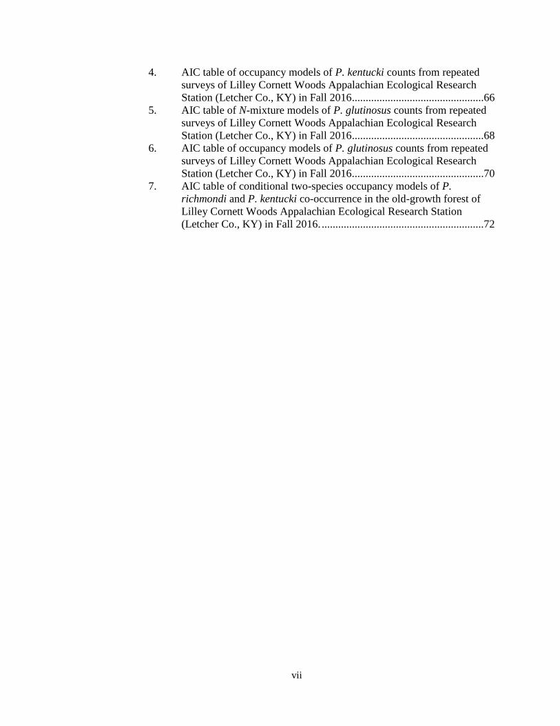
4. AIC table of occupancy models of P. kentucki counts from repeated

surveys of Lilley Cornett Woods Appalachian Ecological Research

Station (Letcher Co., KY) in Fall 2016................................................66

5. AIC table of N-mixture models of P. glutinosus counts from repeated

surveys of Lilley Cornett Woods Appalachian Ecological Research

Station (Letcher Co., KY) in Fall 2016................................................68

6. AIC table of occupancy models of P. glutinosus counts from repeated

surveys of Lilley Cornett Woods Appalachian Ecological Research

Station (Letcher Co., KY) in Fall 2016................................................70

7. AIC table of conditional two-species occupancy models of P.

richmondi and P. kentucki co-occurrence in the old-growth forest of

Lilley Cornett Woods Appalachian Ecological Research Station

(Letcher Co., KY) in Fall 2016. ...........................................................72

viii

LIST OF TABLES

TABLE PAGE

Table 1. Description and summary statistics of covariates used in occupancy and N-

mixture models of three species of woodland salamanders surveyed in 2016 at Lilley

Cornett Woods Appalachian Ecological Research Station (Letcher Co. Kentucky,

USA) ..................................................................................................................................13

Table 2. Results from 10,000 parametric bootstrap goodness-of-fit tests of global

occupancy and N-mixture models (fitted with Poisson distributions) of three species of

Plethodon salamanders surveyed in 2016 at Lilley Cornett Woods Appalachian

Ecological Research Station (Letcher Co., Kentucky, USA) ............................................19

Table 3. Model-averaged predictions of metrics of conditional capture probability and

effective detection probability of three species of Plethodon salamanders from repeated

(N=4) surveys in 2016 at Lilley Cornett Woods Appalachian Ecological Research Station

(Letcher Co., Kentucky, USA) ..........................................................................................25

Table 4. Estimates of availability and temporary emigration derived from model-

averaged estimated detectability parameters of three species of Plethodon salamanders

from repeated (N=4) surveys in 2016 at Lilley Cornett Woods Appalachian Ecological

Research Station (Letcher Co., Kentucky, USA) ..............................................................25

Table 5. Model-averaged predictions from occupancy and N-mixture models of three

species of Plethodon salamanders from repeated (N=4) surveys in 2016 at Lilley Cornett

Woods Appalachian Ecological Research Station (Letcher Co., Kentucky, USA) ...........26

ix

LIST OF FIGURES

FIGURE PAGE

Figure 1. Study location: Lilley Cornett Woods Appalachian Ecological Research

Station ..................................................................................................................................8

Figure 2. Kernel density plot of the elevational distribution of amphibian sampling plots

(N=40) in Shop Hollow at Lilley Cornett Woods Appalachian Ecological Research

Station, Letcher County, Kentucky, USA ............................................................................9

Figure 3. Diagrammatic representation of the workflow process of modeling population

parameters: detectability metrics, occupancy probability, and abundance in Plethodon

salamanders at Lilley Cornett Woods Appalachian Ecological Research Station, Letcher

County, Kentucky, USA ....................................................................................................17

Figure 4. Relationship of salamander mass adjusted for snout-to-vent (SVL) length

(grams per centimeter) and surface microhabitat temperature (degrees Celsius) of

Plethodon richmondi (black), P. kentucki (grey), and P. glutinosus (white) in an old-

growth forest of Lilley Cornett Woods Appalachian Ecological Research Station (data

collected 15 October to 13 November 2016) .....................................................................22

Figure 5. Temperature differentials of microhabitats inhabited by Plethodon salamanders

and ambient (inhabited + uninhabited) in an old-growth forest of Lilley Cornett Woods

Appalachian Ecological Research Station from 15 October to 13 November 2016 ..........23

Figure 6. Model-averaged estimates of effect sizes, β , of covariates used in occupancy

(ψ, dark grey) and N-mixture models (λ, light grey) of Plethodon richmondi (top),

kentucki (middle), and glutinosus (bottom) surveyed at Lilley Cornett Woods

Appalachian Ecological Research Station, Letcher County, Kentucky, USA in Fall

2016....................................................................................................................................28

Figure 7. Model-averaged estimates of occupancy probability (ψ ) of Plethodon

richmondi (A), P. kentucki (B), and P. glutinosus (C) in old-growth forest at Lilley

Cornett Woods Appalachian Ecological Research Station, Letcher County, Kentucky,

USA in Fall 2016 ...............................................................................................................29

Figure 8. Estimates of P. richmondi and P. kentucki co-occurrence from conditional two-

species occupancy models of salamanders surveyed in an old-growth forest at Lilley

Cornett Woods Appalachian Ecological Research Station, Letcher County, Kentucky,

USA in Fall 2016 ...............................................................................................................30

Figure 9. Model-averaged abundance estimates from N-mixture models (extrapolated to 1

ha) of woodland salamanders in an old-growth forest at Lilley Cornett Woods

Appalachian Ecological Research Station, Letcher County, Kentucky, USA in Fall

2016....................................................................................................................................32

1

CHAPTER I

INTRODUCTION

Observations of biological patterns along physical gradients form the foundation

of modern ecology and biogeography (e.g. Hutchinson 1957, MacArthur & Pianka 1966,

MacArthur & Wilson 1967, Simberloff 1974), and a functional understanding of the

mechanisms responsible for these patterns is crucial for the preservation of biodiversity

(Gaston 2000, Willig et al. 2003). Furthermore, analyzing the distribution and abundance

of species along environmental gradients yields invaluable information about their niche

requirements (Costa et al. 2008), population dynamics (Peterman & Semlitsch 2013), and

biotic interactions (Maestre et al. 2009), and can even inform decisions about the

management and restoration of landscapes for species conservation (Peterson 2006).

However, human-altered landscapes may not provide the spectrum of environmental

conditions necessary to fulfill the collective niche requirements of a community

(Oksanen & Minchin 2002, Estavillo et al. 2013). In unaltered landscapes, the

distribution of species is a function of natural environmental gradients, which include

abiotic factors (e.g. surface temperature, moisture, topographic relief, water and soil

chemistry, and solar radiation) and biotic factors (e.g. vegetative structure and presence

of predators, prey, and mates). Taxa likely to exhibit strong responses to such natural

gradients are those with limited dispersal capabilities (Cushman 2006), low reproductive

success (Elton 2000), and acute sensitivity to environmental conditions (Buckley & Jetz

2007).

One such group, amphibians, is particularly responsive to environmental gradients

(Araújo et al. 2007, Werner et al. 2007, Semlitsch et al. 2015). Because of their highly

2

permeable skin, amphibians are acutely sensitive to the chemical environment (Boone et

al. 2007, Willson et al. 2012), thermal and hydrologic regimes (Walls et al. 2013,

Semlitsch et al. 2015), and the microbiome (i.e. emerging pathogenic diseases; Carey et

al. 2003, Collins et al. 2003). As carnivorous ectotherms, amphibian population

dynamics are closely tied to landscape structure (Hecnar & M’Closkey 1996, Rothermel

& Semlitsch 2002) as well as prey availability (Greene et al. 2008), making them

especially sensitive to habitat destruction and degradation (Brooks et al. 2002). These

characteristics likely explain why amphibians are currently experiencing unprecedentedly

precipitous declines on a global scale (Houlahan et al. 2000, Alford et al. 2001, Stuart et

al. 2004). Nevertheless, amphibians’ hypersensitivity to environmental conditions

translates into an effective taxonomic indicator of ecosystem integrity (Welsh & Ollivier

1998, Welsh & Droege 2001).

Despite this sensitivity, amphibians represent a tremendous component of

biomass in aquatic (Gibbons et al. 2006), terrestrial (Burton & Likens 1975b, Petranka &

Murray 2001), and riparian (Peterman et al. 2008) ecosystems. Because the life history of

many amphibians involves movement between and among aquatic and terrestrial

ecosystems (Regester et al. 2006), they are responsible for the transformation (Burton &

Likens 1975a) and translocation (Capps et al. 2014, Luhring et al. 2017) of substantial

quantities of energy throughout the landscape. However, the role of energy

transformation is not unique to biphasic organisms.

Terrestrial woodland salamanders (Caudata: Plethodontidae: Plethodon), which

lack aquatic larval stages (i.e. have direct development), are among the most abundant

vertebrate animals in eastern deciduous forests of North America (Petranka & Murray

3

2001, Semlitsch et al. 2014)—reaching densities between 0.73 and 18.46 individuals per

m2 (Semlitsch et al. 2014, O’Donnell & Semlitsch 2015). They also act as predators of

detrital food webs (Best & Welsh 2014, Hutton et al. 2017, Davic & Welsh 2004) and

represent a prey resource for a wealth of vertebrate and invertebrate predators (for a

taxonomic review of Plethodon predators, see Semlitsch 2014). As such, woodland

salamanders are hypothesized to serve as a key energetic intermediary between highly

disparate levels of trophic organization in terrestrial ecosystems (detrital communities

and high-order vertebrate predators; Burton & Likens 1975b) and exert a significant, top-

down, regulatory force upon detrital food webs, leaf litter decomposition, and organic

material retention (Burton & Likens 1975a, Hairston 1987). Therefore, woodland

salamanders may significantly influence the direction and magnitude of energy flow

through ecosystems (Davic & Welsh 2004).

Wyman (1998) found that, through predation of detrital food webs, woodland

salamanders (Plethodon cinereus, eastern red-backed salamander) can indirectly reduce

leaf-litter processing rates by 11–17%, aiding in the retention of organic carbon in

forests, and perhaps even reducing gaseous carbon fluxes into the atmosphere via

heterotrophic decomposition of organic material. Additional studies with terrestrial

salamanders (Plethodontidae) have found that the strength and sign of top-down effects

on leaf litter decomposition and detrital communities is subject to variation (Walton

2005, Walton & Streckler 2005, Walton et al. 2006, Homyack et al. 2010, Best & Welsh

2014). Recent evidence suggests that variation in the effects of terrestrial salamanders on

forest floor dynamics is likely correlated with spatio-temporal variability in

environmental conditions (Walton 2013) and the abundance of salamander predators

4

(Hickerson et al. 2017). Walton (2013) found that patterns in leaf litter mass and moisture

predicted the effects of terrestrial salamanders on detrital food webs; increasing litter

mass may amplify the predatory effect of salamanders on invertebrate prey, while

increasing litter moisture may buffer such predatory effects. Hickerson et al. 2017 found

that increased salamander abundance corresponded with slower rates of leaf litter

decomposition, which contributes to higher organic material retention in terrestrial

ecosystems (Aerts 1997). Therefore, the nature of woodland salamanders’ role in

terrestrial ecosystem nutrient cycling is likely contingent upon the spatial distribution of

their biomass within the ecosystem (Hickerson et al. 2017, Semlitsch et al. 2014), which

is influenced by spatial patterns in environmental conditions and resource availability

(Walton 2013, Peterman & Semlitsch 2013, Milanovich & Peterman 2016).

Numerous studies have found the distribution of woodland salamanders to be

influenced chiefly by terrestrial ecosystem features such as soil moisture (Jaeger 1971a,

Wyman 1988, Peterman & Semlitsch 2013), availability of natural cover (i.e. coarse

woody debris, rocky cover, and leaf litter; McKenny et al. 2006, O’Donnell et al. 2014),

and forest composition/canopy structure (Gibbs 1998, Peterman & Semlitsch 2013).

Furthermore, presence of heterospecifics has been found to influence microhabitat usage

(Keen 1982, Farallo & Miles 2016), distribution (Hairston 1950, Jaeger 1970, 1971a,

1972b), and abundance (Hairston 1951) of individual species. Thus, the species-specific

contribution of woodland salamanders to terrestrial ecosystem processes may be modified

through population-level effects of interspecific competition. Due to the diversity and

endemism of woodland salamanders, particularly in Appalachian forests, where their

diversity is greatest (Dodd 2004), community structure varies dramatically across

5

physiographic regions. Therefore, community interactions are likely geographically

nuanced and not easily generalizable from any single region.

With the desire to further understand the inherent complexity of woodland

salamander ecology in Appalachian forests, descriptions of veritable detail have been

repeatedly published for well over a century (e.g. Cope 1870, Brimley 1912, King 1939,

Hairston 1949, Highton 1972, 1995, Dodd 2004), and these observations are paramount

to our knowledge of woodland salamander natural history and ecology. However, many

studies used occurrence records, either from field surveys or natural history collections,

and count indices to approximate the distribution and abundance of woodland

salamanders (Anderson 2001; although see McKenny et al. 2006, Peterman & Semlitsch

2013, Semlitsch et al. 2014). Certain aspects of woodland salamander natural history,

such as subsurface migration (temporary emigration) and crypsis, when combined with

the ability (or inability) of observers to detect a species, allow salamanders to occupy a

patch without being detected (Hyde & Simons 2001, Bailey et al. 2004). Therefore, a

lack of detection does not always imply absence. Likewise, in many circumstances the

perceived abundance of a species is confounded by numerous variables, including some

biological (e.g. crypsis, emigration, foraging and breeding behavior; Durso et al. 2011,

O’Donnell & Semlitsch 2015), some environmental (e.g. precipitation, season, surface

temperature, abundance of cover items; Hyde & Simons 2001, Guzy et al. 2014), and

some human (observer experience, visual/auditory acuity, search vigor; Simons 2007).

Therefore, species counts often serve insufficiently as indices of abundance. Central to

these issues is the concept of imperfect detection (Gu & Swihart 2004): detection is

seldom perfect and often covaries predictably with certain factors. Fortunately, modeling

6

the distribution and abundance of species while accounting for imperfect detection is now

possible without the implementation of invasive and expensive capture-mark-recapture

methods through the use of hierarchical models of occupancy and abundance

(MacKenzie et al. 2002, Royle 2004, Pellet & Schmidt 2005, Kéry & Royle 2016).

Hierarchical models allow the estimation of population parameters (distribution and

population density), while simultaneously incorporating heterogenous detection

probabilities.

Studies of the spatial population dynamics of woodland salamander species

occurring in syntopy, which incorporate imperfect detection, are needed to further

understand the role of these animals in terrestrial ecosystems. Furthermore, woodland

salamander populations in lower elevation Appalachian forests, like those of central

Appalachia, have not been studied as thoroughly as in regions with greater topographic

relief and higher proportions of land allocated for conservation (i.e. Piedmonts, Blue

Ridge, southwestern Appalachia). Therefore, this study examines the population

dynamics of an assemblage of woodland salamanders—P. richmondi, P. kentucki, and P.

glutinosus—within an old-growth forest in the Cumberland Plateau region of Appalachia.

The objectives of this study were to (1) determine if natural environmental

gradients associated with the transition from mesic to xeric forest habitat within

Appalachian forest influence the microhabitat use, fine-scale distribution, and abundance

of woodland salamanders, (2) determine if those relationships vary among species. These

objectives were addressed by assessing the microhabitat of woodland salamanders and

constructing models of occupancy and abundance, incorporating imperfect detection,

from temporally-replicated surveys within an old-growth forest in eastern Kentucky.

7

CHAPTER II

METHODS

Study Site

This study was conducted at Lilley Cornett Woods Appalachian Ecological

Research Station (LCW), which contains 102-ha of old-growth forest (Figure 1). Lilley

Cornett Woods is a stable mixed mesophytic forest in the Cumberland Plateau region of

southeastern Kentucky. The dissected topography of this region greatly modifies local

climate and generates a gradient of soil moisture, depth, and complexity, resulting in high

botanical diversity (Braun 1950, Chapman & McEwan 2013). Martin (1975) described

nine upland forest communities in LCW, composed chiefly of several beech

communities, as well as oak, sugar maple-basswood-tulip poplar, and hemlock

communities. Generally, mesic habitats are found on north-to-east facing slopes with

minimal convexity and feature deep soils, rich with organic matter; xeric habitats are

represented on most south-to-west facing slopes and ridge tops, and contain shallow soil

horizons dominated by clay (pers. obs., Martin 1975). With no history of timber harvest

the old-growth forest at LCW has experienced virtually no substantial anthropogenic

disturbance with the exception of understory livestock grazing, which ended in the 1950s.

Of the three tracts of old-growth forest at LCW, one tract, “Shop Hollow”, (Figure 1,

panel E) currently experiences little disturbance from human recreation (only guided

hiking on an established trail) and invasive plants (J. Peters, unpubl. data), and was

therefore chosen as the location for this study. Shop Hollow features 57 permanent 0.08-

ha circular sample plots, originally established by Martin (1975). Sample plots are

stratified by aspect and slope (lower [< 345 m], middle [345–410 m], upper [411–467 m],

8

and ridge [> 467 m]; Figure 2). Data collection occurred at all sample plots free of

intersecting streams (N=40; Figure 1), and plots contained relatively minimal understory

vegetation.

Figure 1. Study location: Lilley Cornett Woods Appalachian Ecological Research Station.

(A) County map of Kentucky, USA, (B) Letcher County, KY, (C) Boundary of old-growth

forest at Lilley Cornett Woods Appalachian Ecological Research Station (LWC), (D)

Terrain map of LCW; points represent amphibian sampling locations (N=40), (E) 0.08-ha

circular sample plots in the Shop Hollow stand of LCW.

Amphibian Sampling

LCW features three species of Plethodon (Caudata: Plethodontidae) salamander

found throughout much of the Cumberland Plateau region: Plethodon glutinosus

(northern slimy salamander, Green 1838), P. kentucki (Cumberland Plateau salamander,

9

Mittleman 1951), and P. richmondi (southern ravine salamander,

Netting & Mittleman 1938). Additional genera (Desmognathus, Pseudotriton,

Gyrinophilus, Eurycea, and Ambystoma) were not captured frequently enough to merit

further analysis.

Figure 2. Kernel density plot of the elevational distribution of amphibian sampling plots

(N=40) in Shop Hollow at Lilley Cornett Woods Appalachian Ecological Research Station,

Letcher County, Kentucky, USA.

This study relied upon visual encounter surveys (VES) to detect species, and

therefore all observations resulted from hand captures during standardized searching.

Sampling events consisted of four two-day intervals occurring from 15 October to 13

November 2016. Surveys were conducted along a linear 3-m x 36-m transect through the

center point of each 0.08-ha circular sample plot. To eliminate sampling bias and ensure

plots were sampled thoroughly, the direction of VES transects during every sampling

10

event was determined by randomly selecting a bearing between 0° and 180°, with the

midpoint of all transects pivoting at the geometric center of the circular sample plot. In

LCW, woodland salamanders are found primarily by searching under coarse woody

debris, rocks, and other natural cover on the forest floor. Moist leaf litter may also

provide suitable habitat, but preliminary surveys with comparable effort yielded

substantially fewer captures. During surveys, all coarse woody debris and rocky cover

within the 96 m2 were flipped, and microhabitats beneath were examined for the presence

of salamanders before replacing cover items to their exact position. Microhabitat

temperature was recorded temperature under every cover item within the sampling

transect using a handheld infrared thermometer (Kintrex, model: IRT0421).

Microhabitats inhabited by salamanders were noted to allow for a comparison of

temperatures between inhabited, uninhabited, and inhabited + uninhabited (ambient)

microhabitats. Microhabitat moisture was recorded only under cover objects inhabited by

salamanders using a moisture probe (Decagon Devices, model: Pro Check). Once

captured, snout-to-vent length (SVL) and tail length (TL) were measured by placing the

animal in a clean plastic bag and measuring from the tip of the snout to the posterior edge

of the vent (accuracy = 1 mm), and mass was recorded using 10-g or 20-g PESOLA scale

(accuracy = 0.1 g and 0.2 g, respectively). Following data collection animals were

returned to their precise capture location. All protocols for the use and handling of

amphibians were approved by the Eastern Kentucky University Animal Care and Use

Committee (IACUC protocol # 05-2015).

11

Site Covariates

Soil moisture of each sampling plot was measured during every survey at five

equidistant points along the transect using a Pro Check moisture probe (Decagon

Devices, Inc.). Moisture data were then averaged across sites and surveys to obtain an

accurate estimate of site-level variation in soil moisture within the sampling season.

Quantification of forest canopy openness was achieved using hemispherical canopy

photography (Herbert 1987, Frazer et al. 1997; Baldwin et al. 2006). Canopy structure

was captured with a 24-megapixel digital single lens reflex camera (Nikon D7100), fitted

with a 180° lens (Nikon AF DX Fisheye-Nikkor 10.5 mm f/2.8G ED; Nikon Instruments,

Melville, NY, U.S.A.). The camera was adjusted using a leveling tripod, and photographs

were taken on automatic settings with the camera angled vertically at the underside of the

canopy. All photographs were taken during the fall of 2016, just prior to leaf off. Percent

canopy openness was calculated by converting images into binary color (black pixels =

closed canopy, white pixels = open canopy) using a binarization algorithm provided by

the Auto Threshold Plugin for ImageJ software (Abramoff et al. 2004, Rasband 2014),

and then calculating the percent of white pixels in each frame.

A GIS and remotely sensed data were used to gather several reportedly useful

covariates for modeling population parameters of woodland salamanders: aspect,

elevation, slope, topography, canopy, and solar radiation (Hairston 1951, Ford et al.

2002, Peterman & Semlitsch 2013, Semlitsch et al. 2014). See Table 1 for a description

of all site covariates. A 1.11-m2 digital elevation model was used to derive the following

layers: aspect, slope, Topographic Position Index, and Direct Solar Radiation. Aspect was

scaled into a linear variable ranging from 0 (xeric, southwest-facing slopes) to 2 (mesic,

12

northeast-facing slopes) using the Beers transformation (Beers et al. 1966, O’Donnell et

al. 2015a). Topographic Position Index (TPI) is the slope position of sample plots relative

to surrounding landscape. It was calculated using a neighborhood function, which

calculates changes in DEM cells within a chosen, 150-m, buffer of the sample site

(Guisan & Weiss 1999, Weiss 2001). Direct Solar Radiation, a component of the total

solar radiation, represents the quantity of solar radiation remaining after a fraction is

absorbed by the atmosphere (diffuse solar radiation) or reflected off of the earth’s surface

(reflected solar radiation). Normalized Difference Vegetation Index (NDVI) is a measure

of vegetative cover (range: -1.0 [barren] to 1.0 [heavily vegetated]), and was derived

using imagery from the National Agriculture Imagery Program. All data were gathered

and analyzed with ArcGIS 10.3 (ESRI 2011).

13

Table 1: Description and summary statistics of covariates used in occupancy and N-mixture models of three species of woodland

salamanders surveyed in 2016 at Lilley Cornett Woods Appalachian Ecological Research Station (Letcher Co., Kentucky,

U.S.A.). Covariates quantify two important processes: "sampling" (detectability) and "site" (species occupancy or population size).

14

Sampling Covariates

The quantity of fallen coarse woody debris larger than 20 cm in diameter (Muller

and Liu 1991) and rocky cover within each VES transect were counted. Leaf-litter depth

was measured with a metric ruler at five equidistant points within each survey transect.

Solar conditions during surveys were quantified by measuring the ambient luminous flux

(perceived power of light) at breast height with a digital illuminance light meter

(TekPower, model: LX1330B). Finally, date and time of day of each survey was

recorded. See Table 1 for a description of all sampling covariates.

Data Analysis

To test the hypothesis that microhabitat use differs among the three species of

woodland salamanders at LCW, the average temperature and soil moisture content of

each species’ refugia was compared using a two-way ANOVA (α = 0.05), and if

differences were detected, multiple comparisons were made using a Tukey’s honest

significant difference (HSD) test. The hypothesis that salamanders are selecting

microhabitats with temperatures that differ from ambient microhabitat temperature was

tested by comparing average temperatures of microhabitats occupied by each species

with the average temperature of all available microhabitat (occupied + unoccupied)

within the transect using independent t-tests (α = 0.05). Additionally, an ordinary least

squares regression was used to determine if salamander body mass adjusted for SVL

predicted microhabitat temperature (α = 0.05). A two-way ANOVA (α = 0.05), followed

by a Tukey HSD test, was used to determine differences in salamander body masses by

species. All statistical procedures were performed in the R programming environment (v.

3.4.1; R Core Team 2017).

15

Because detection probabilities of salamanders were assumed <1, hierarchical

models (HMs) were used to approximate woodland salamander distributions and

population size from repeated surveys of unmarked animals (MacKenzie & Royle 2005).

One of the most restrictive assumptions of HMs is population closure. In the context of

HMs used for occupancy (occupancy models), the state parameter—whether a species is

present or absent—must remain static during and between surveys (i.e. closed to

migration, extinction, and colonization). The population closure assumption for HMs of

abundance (N-mixture models) restricts any net flux in population size, and therefore

populations must remain closed to births, deaths, migration, extinction, and colonization.

While exhaustive, these assumptions can be met by conducting field surveys in rapid

succession, minimizing the duration between surveys (MacKenzie & Royle 2005,

MacKenzie et al. 2006). Therefore, the sampling design of this study satisfied these

assumptions.

Although occupancy and N-mixture models both require an estimate of

detectability to compute state parameters, the specific components of detection used by

each are surprisingly different (O’Donnell and Semlitsch 2015). Most occupancy models,

including the model used in this study, estimate the “conditional capture probability”

(pψ), defined as the probability of capture, given the individual is present (capture

probability | availability). For these terms, availability is defined as 1 – (temporary

emigration). N-mixture models estimate a form of detection which combines a term for

the ability of the observer to capture an individual that is present (conditional capture

probability) with a term for the individual’s availability for capture (expressed as:

16

availability x conditional capture probability), and is thus referred to as an “effective

detection probability” (pλ).

Occupancy models (MacKenzie et al. 2002) were used to estimate the probability

that a species occupied a given site (ψ), while N-mixture models (Royle 2004) were used

to estimate species true population size (λ). Fitting occupancy and N-mixture models

followed a stepwise procedure (Kendall et al. 2009, Scherer et al. 2012, Peterman &

Semlitsch 2013, O’Donnell et al. 2015b; see Figure 3 for workflow diagram): (1) models

were constructed to estimate detection probabilities by holding the state parameters, ψ

and λ, constant (Appendices 1–6); (2) the model-averaged effects (β ) of each p covariate

was calculated using multi-model inference (Burnham & Anderson 2002, Mazerolle

2006) to determine importance; (3) models with a single site covariate were then

constructed to estimate ψ and λ using p covariates selected from the previous step; (4)

from the resulting models, β was calculated for each site covariate to determine which

was important in explaining ψ and λ; (5) if two or more site covariates featured

significant β estimates (95% CI not containing “0”), models containing two site

covariates were run and β recalculated; (6) all models were ranked and multi-model

inference was used to make predictions across all models. Models failing to converge or

exhibiting signs of instability (producing inflated confidence intervals, arbitrarily large

standard errors, or non-numeric predictions) were discarded.

17

Figure 3. Diagrammatic representation of the workflow process of modeling population

parameters: detectability metrics, occupancy probability, and abundance in Plethodon

salamanders at Lilley Cornett Woods Appalachian Ecological Research Station, Letcher

County, Kentucky, USA.

18

Prior to fitting, all site and sampling covariates were standardized to a mean of

zero and unit variance by subtracting the arithmetic mean and dividing by the standard

deviation (as recommended by Fiske & Chandler 2011, 2017). Occupancy and N-mixture

models were fitted using a maximum-likelihood approach with package “unmarked”

(Fiske & Chandler 2011), in the R programming environment (v. 3.4.1; R Core Team

2017). Goodness-of-fit tests with 10,000 parametric bootstrap iterations on a Chi-square

discrepancy were performed on the most highly parameterized (global) occupancy and N-

mixture models of each species to assess model adequacy and check for overdispersion,

as recommended by Kéry & Royle (2016). These tests confirmed that each species’

occupancy and N-mixture models, barring one, performed well under standard

parameterization, with little or no evidence of lack of fit (p > 0.05, c ≈ 1; Table 2).

Perhaps due to sparse detections, the N-mixture model for P. glutinosus was moderately

overdispersed (c = 1.92, Table 2; Kéry & Royle. 2016). Alternative negative binomial

(NB) and zero-inflated Poisson (ZIP) distribution models were both fitted and compared

to the Poisson distribution model originally created. Additional goodness-of-fit tests

determined a ZIP distribution produced the least over-dispersed model (p = 0.226, c =

1.357), surpassing that of NB (p = 0.231, c = 1.380), and therefore ZIP distributions were

used for all N-mixture models of P. glutinosus. All resultant occupancy and N-mixture

models were ranked with AIC (Appendices 1–6), model-averaged, and back-transformed

to obtain predictions. Multi-model inference, back-transformations, and goodness-of-fit

tests were all executed using R package “AICcmodavg” (Mazerolle 2015).

19

It was further hypothesized that (1) the distribution of woodland salamanders in

LCW is modified behaviorally through interspecific competition and territoriality, and (2)

the pattern of co-occurrence of woodland salamanders varies along natural environmental

gradients. To test these hypotheses, two-species occupancy models were used to

investigate patterns of co-occurrence (MacKenzie et al. 2004). The necessarily complex

parameterization scheme of co-occurrence models featuring P. glutinosus, which was

infrequently detected during this study, resulted in lack of model convergence. Therefore,

co-occurrence models were only performed on P. richmondi and P. kentucki. The two-

species occupancy model—an extension of the MacKenzie et al. (2002) single-species

occupancy model—estimates the probability of two species occupying a patch

simultaneously, while accounting for species-specific detection probabilities. To integrate

effects from environmental gradients (i.e. site covariates) into the models of co-

occurrence, an alternate parameterization of the MacKenzie (2004) model developed by

Richmond et al. (2010) was used (known as the “conditional two-species occupancy

model”). As opposed to the single-species occupancy model, this model allows for

estimation of many additional population parameters, including the two-species joint

conditional occupancy probability, or co-occurrence probability—the probability of a

χ2

c p χ2

c p

P. richmondi 15.96 1.18 0.263 144.12 0.96 0.583

P. kentucki 15.28 1.14 0.299 169.40 1.13 0.148

P. glutinosus 6.71 0.83 0.393 139.12 1.92 0.099

ψ λ

χ2 = Pearson chi-square statistic, c = overdispersion estimate, p = p-value

Table 2: Results from 10,000 parametric bootstrap goodness-of-fit tests of global occupancy and

N-mixture models (fitted with Poisson distributions) of three species of Plethodon salamanders

surveyed in 2016 at Lilley Cornett Woods Appalachian Ecological Research Station (Letcher Co.,

Kentucky, USA).

ψ = conditional occupancy probability, λ = estimated population size,

Species

20

given species, SA, occupying a site or sites wherein another species, SB, is known to be

present. Under the null hypothesis, the pattern and frequency of species co-occurrence

does not vary across environmental gradients. This hypothesis was tested by comparing a

null model of co-occurrence, wherein the pattern in which species co-occur at sites is

unrelated to environmental conditions (essentially random), to models of co-occurrence

which predict co-occurrence patterns relating to environmental gradients. Using the co-

occurrence probability (ψAB), a “Species Interaction Factor”, or φ, can also be obtained

(MacKenzie 2004, Richmond et al. 2010). For species A and B, φ is defined as:

φ = ψAB

ψA۰ψB

;

where ψA and ψB are the independent occupancy probabilities of species A and B, and

ψAB represents the co-occurrence probability of species A and B. Under the null

hypothesis, φ = 1, species populations exist independently and the pattern and frequency

of species co-occurrence is assumed to be random. If φ > 1, species co-occur more

frequently than expected from chance; likewise, φ < 1 indicates species occur less

frequently than chance.

Conditional two-species occupancy models (hereafter referred to as “co-

occurrence models”) were constructed to investigate if populations of P. richmondi and

P. kentucki experience competition and if co-occurrence patterns vary across

environmental gradients. Co-occurrence models were parameterized using the site and

sampling covariates previously identified as important in single-species occupancy

models (Appendices 1–6). Candidate models were fitted within the maximum-likelihood

framework provided by program PRESENCE (v. 11.7; Hines 2006) under a ψBa-

parameterization (Richmond et al. 2010) and ranked using AIC (Appendix 7).

21

CHAPTER III

RESULTS

Repeated surveys of woodland salamanders at LCW resulted in the

capture of 55 P. richmondi, 46 P. kentucki, and 8 P. glutinosus, with an average of 27.25

captures per survey. Plethodon glutinosus were only detected at 7 of 40 sites (naïve

proportion of area occupied [POA] = 0.18), while P. richmondi and P. kentucki were

detected at 25 and 26 of the total 40 sites surveyed, respectively (POA: P. richmondi =

0.63, P. kentucki = 0.65). An average of 2.73 salamanders were detected at each site

(inter-quartile range [IQR] = 1.00–5.00), with a maximum of 11 detections and nine sites

with zero detections.

Body Size and Microhabitat Usage

Some differences were found between the body size (defined as salamander mass

adjusted for snout-to-vent [SVL] length) of each species (F2,104 = 5.954, p < 0.004).

Plethodon glutinosus was 3.7–7.2 g۰cm-2 greater than P. kentucki (p = 0.043) and 4.9–8.4

g۰cm-2 greater than P. richmondi (p = 0.004), however no differences were found

between body sizes of P. richmondi and P. kentucki (p = 0.192; Figure 4). Body size was

considered as a predictor of microhabitat moisture and temperature. Volumetric moisture

content of microhabitats inhabited by each species did not vary significantly (F2,100 =

0.7942, p = 0.4548; IQR = 0.174–0.211 m3۰m-3). However, body size was a significant

predictor of microhabitat temperature (F1,105 = 10.533, p = 0.002, R2 = 0.09), suggesting

that large bodied Plethodon tolerate higher temperatures (Figure 4).

22

Figure 4: Relationship of salamander mass adjusted for snout-to-vent (SVL) length (grams

per centimeter) and surface microhabitat temperature (degrees Celsius) of Plethodon

richmondi (black), P. kentucki (grey), and P. glutinosus (white) in an old-growth forest of

Lilley Cornett Woods Appalachian Ecological Research Station (data collected 15 October

to 13 November 2016). Dotted line represents a least squares regression of microhabitat

temperature and SVL-adjusted biomass (F1,105 = 10.533, p = 0.002). Horizontal boxplots

above regression display summaries of SVL-adjusted biomass by species; letters beside

boxplots denote statistically significant groups (Tukey HSD) from a two-way ANOVA

(F2,104 = 5.954, p < 0.004).

Temperature of microhabitats inhabited by P. richmondi, P. kentucki, and P.

glutinosus differed significantly (F2,104 = 5.954, p = 0.004). Plethodon glutinosus

inhabited microhabitats 1.34–8.39 ℃ warmer (Tukey 95% CI) than P. richmondi (p =

0.004) and 0.09–7.22 ℃ warmer than P. kentucki (p = 0.043). There was no evidence to

suggest that P. richmondi and P. kentucki inhabited microhabitats with different

temperatures (p = 0.191). While microhabitat temperature of P. kentucki did not differ

from ambient microhabitat conditions (t = -1.157, d.f. = 55.37, p = 0.271), P. richmondi

23

and P. glutinosus were significantly different from ambient temperature. Microhabitats

inhabited by P. richmondi were 0.79–2.78 ℃ cooler than ambient temperature (t = -3.590,

d.f. = 61.86, p < 0.001) and those of P. glutinosus were 0.97–5.18 ℃ warmer (t = 3.705,

d.f. = 5.24, p = 0.013; Figure 5).

Figure 5: Temperature differentials of microhabitats inhabited by Plethodon salamanders

and ambient (inhabited + uninhabited) in an old-growth forest of Lilley Cornett Woods

Appalachian Ecological Research Station from 15 October to 13 November 2016. Lateral

boundaries of boxplots represent kernel density estimates. Letters above boxplots denote

statistically significant groups (Tukey HSD) from a two-way ANOVA (α = 0.05) of

microhabitat temperature between three species of Plethodon. P-values accompanying

each line segment drawn between plots are resultant from independent t-tests (α = 0.05) of

microhabitat occupied by each Plethodon species and ambient microhabitat. NS indicates

a statistical test with p > 0.05. Left-sided rug marks (in gray) represent values of

observations from inhabited microhabitats and right-sided represent those of ambient

microhabitats with 10% thinning to increase visibility.

24

Detection, Availability, and Temporary Emigration

All detection probability estimates reported herein are model-averaged across the

full candidate set of models. Plethodon richmondi and P. kentucki exhibited moderately

low detection probabilities, while detection of P. glutinosus was extremely low (Table 3).

Additionally, for P. richmondi and P. kentucki, p ψ far exceeded p λ. On the contrary, P.

glutinosus p ψ was approximately equivalent to p λ, suggesting availability ≈ 1. For P.

richmondi, time of day (“TOD”) in which the survey occurred was the most important

covariate for estimating conditional capture probability (β ψ = -0.42 [95% unconditional

CI: -0.83, -0.01]) and effective detection probability (β λ = -0.43 [-0.75, -0.12]).

Availability of coarse woody debris (“CWD”) was the most important covariate in

explaining both detectability parameters of P. kentucki (β ψ = -0.42 [-0.83, -0.01, β λ = -

0.43 [95% CI: -0.75, -0.12]). Two covariates, TOD and CWD, explained the conditional

capture probability (β ψ, TOD = 1.45 [0.41, 2.49], β ψ, CWD = 1.41 [0.48, 2.33]) and effective

detection probability (β λ, TOD = 1.19 [0.33, 2.05], β λ, CWD = 1.14 [0.47, 1.82]) of P.

glutinosus; however, to avoid model nonconvergence due to over-parameterization,

models were parameterized with a maximum of one covariate per parameter (all

occupancy and N-mixture models have K ≤ 4). Therefore, the covariate with the smallest

β 95% unconditional CI was used to estimate state parameters (CWD for ψ, TOD for λ).

25

By exploiting the relationship between effective detection probability and

conditional capture probability, a population’s availability for capture and temporary

emigration (probability an animal is alive, but unavailable for capture), can be obtained

mathematically (Table 4). Derivations from two components of detectability estimated

within this study reveal that P. richmondi and P. kentucki both exhibit relatively low

availability for capture and relatively high temporary emigration when compared to P.

glutinosus (Table 4).

Occupancy

Plethodon richmondi was predicted to have the most restricted distribution, with a

model-averaged estimate of occupancy probability, ψ , of 0.737 (95% CI: 0.35, 0.89).

Comparatively, P. kentucki and P. glutinosus were distributed more ubiquitously (ψ kentucki

lower upper lower upper

P. richmondi 0.355 0.245, 0.486 0.058 0.024, 0.136

P. kentucki 0.243 0.159, 0.349 0.050 0.015, 0.154

P. glutinosus 0.045 0.016, 0.113 0.043 0.001, 0.420

† defined as (capture prob.)|(availability), ‡ defined as (conditional capture prob.) x (availability)

Table 3: Model-averaged predictions of metrics of conditional capture probability and effective

detection probability of three species of Plethodon salamanders from repeated (N=4) surveys in 2016

at Lilley Cornett Woods Appalachian Ecological Research Station (Letcher Co., Kentucky, USA).

Table includes estimates and 95% CI. All values are an average of N=40 sites.

SpeciesConditional capture

probability† (p ψ)

95% CI Effective detection

probability‡

(p λ)

95% CI

P. richmondi 0.355 0.058 0.164 0.836

P. kentucki 0.243 0.050 0.204 0.796

P. glutinosus 0.045 0.043 0.962 0.038

Conditional capture

probability (p ψ)

Effective detection

probability (p λ)

Table 4: Estimates of availability and temporary emigration derived from model-averaged estimated

detectability parameters of three species of Plethodon salamanders from repeated (N=4) surveys in

2016 at Lilley Cornett Woods Appalachian Ecological Research Station (Letcher Co., Kentucky,

USA). All values are an average of N=40 sites.

† derived using the formula: (effective detecton prob.)/(conditional capture prob.), ‡ defined as 1 - (availability)

Species Availability†Temporary

Emigration‡

26

= 0.947 [0.11, 1.0], ψ glutinosus = 0.984 [0.0, 1.0]), although the error surrounding estimates

of P. glutinosus occupancy were large (Table 5).

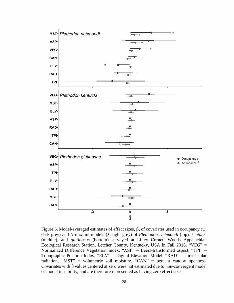
Percent soil moisture (“MST”), NDVI (“VEG”), and elevation (“ELV”)

were all important covariates in estimating occupancy of P. richmondi (β MST = 2.27

[0.11, 4.43]), β VEG = 1.04 [0.07, 2.01], β ELV = -1.27 [-2.46, -0.08]; Figure 6). Like P.

richmondi, P. kentucki and P. glutinosus occupancy was also correlated with % soil

moisture and NDVI (Figure 7), but the directions of the covariates’ effects were

heterogeneous (P. kentucki: β MST = 0.90 [-2.07, 3.89], β VEG = 2.04 [-0.89, 4.97]; P.

glutinosus: β MST = -0.81 [-3.89, 2.28], β VEG = 0.52 [-2.19, 3.22]; Figures 6 and 7). The

remaining covariates included in models of occupancy produced heterogeneous effects

and were therefore not considered to be reliable predictors of woodland salamander

distributions in LCW (Figure 6).

Co-occurrence

Co-occurrence models determined the overall probability of P. richmondi co-

occurring with P. kentucki, ψ ric | ken, was 0.72 (95% CI: 0.53, 0.86). Models of co-

occurrence featuring covariates that represent environmental gradients were better at

predicting patterns of co-occurrence (cumulative Akaike model weight [Σωij] = 0.971)

lower upper upper

P. richmondi 0.737 0.348, 0.895 0.151

P. kentucki 0.947 0.105, 0.997 0.206

P. glutinosus 0.984 0.001, 1.000 < 0.001, 14.808

ψ = estimated occupancy probability, λ = estimated abundance (expressed as density per m-2

)

Table 5: Model-averaged predictions from occupancy and N-mixture models of three species of

Plethodon salamanders from repeated (N=4) surveys in 2016 at Lilley Cornett Woods

Appalachian Ecological Research Station (Letcher Co., Kentucky, USA). Table includes

estimates and unconditional 95% confidence intervals of occupancy probability and density. All

values are an average of N=40 sites.

Species ψ 95% CI

λ ۰m-2 95% CI

lower

0.060 0.025,

0.061 0.019,

0.036

27

than null models (Σωij = 0.029; Appendix 7). Co-occurrence probabilities were positively

influenced by percent soil moisture and NDVI (Figure 8). The relationship of ψ ric | ken with

NDVI was nearly linear, with a gradual positive slope. Co-occurrence exhibited a steep

positive slope where percent soil moisture <15%, plateauing at approximately 20%.

These results provide evidence that species co-occurrence patterns are non-random and

vary along natural environmental gradients. However, the Species Interaction Factor, or

φ, of P. richmondi and P. kentucki was equal to 1 (φ = 1.00; 95% CI = 0.984, 1.016),

which provides evidence that populations of P. kentucki and P. richmondi occur

independently and do not experience competition.

28

Figure 6. Model-averaged estimates of effect sizes, β , of covariates used in occupancy (ψ,

dark grey) and N-mixture models (λ, light grey) of Plethodon richmondi (top), kentucki

(middle), and glutinosus (bottom) surveyed at Lilley Cornett Woods Appalachian

Ecological Research Station, Letcher County, Kentucky, USA in Fall 2016. “VEG” =

Normalized Difference Vegetation Index, “ASP” = Beers-transformed aspect, “TPI” =

Topographic Position Index, “ELV” = Digital Elevation Model, “RAD” = direct solar

radiation, “MST” = volumetric soil moisture, “CAN” = percent canopy openness.

Covariates with β values centered at zero were not estimated due to non-convergent model

or model instability, and are therefore represented as having zero effect sizes.

29

Figure 7. Model-averaged estimates of occupancy probability (ψ ) of Plethodon richmondi

(A), P. kentucki (B), and P. glutinosus (C) in old-growth forest at Lilley Cornett Woods

Appalachian Ecological Research Station, Letcher County, Kentucky, USA in Fall 2016.

Surfaces of three-dimensional plots represent patterns of predicted occupancy probability

with respect to percent soil moisture and NDVI (Normalized Difference Vegetation Index),

an estimate of canopy density gathered from NAIP imagery. Note: change in scale of ψ across species.

30

Figure 8. Estimates of P. richmondi and P. kentucki co-occurrence from conditional two-

species occupancy models of salamanders surveyed in an old-growth forest at Lilley

Cornett Woods Appalachian Ecological Research Station, Letcher County, Kentucky, USA

in Fall 2016. Curves model relation of co-occurrence probability with percent soil moisture

(bottom) and Normalized Difference Vegetation Index (NDVI, top). Gray regions

represent 95% confidence intervals.

31

Abundance

Abundance estimates obtained from N-mixture models were substantially greater

than counts uncorrected for effective detection probability, such that counts only

represented 1.43–7.22 % (inter-quartile range) of the total estimated abundance of all

three species of woodland salamanders. Plethodon richmondi and P. kentucki had similar

estimated densities and were approximately twice as large as those of P. glutinosus

(Table 4); although, 95% unconditional confidence intervals of P. glutinosus abundance

were large and exceeded the upper limits of both P. richmondi and P. kentucki. When

extrapolated to the total extent of the study area (44.25 ha), abundances of Plethodon

species were estimated at Nrichmondi = 26570 (95% CI: 10895, 66897), Nkentucki = 26848

(95% CI: 8552, 91098), and Nglutinosus = 8461.61 (95% CI: 47.55, 2.75۰109).

Percent soil moisture (“MST”) and Beers-transformed aspect (“ASP”) were the

most important covariates when estimating abundance of P. richmondi (β MST = 0.48

[0.14, 0.82]), β ASP = 0.58 [0.1, 1.05]; Figure 6 and 9). Plethodon richmondi abundance

exhibited marked, positive curvilinear responses to percent soil moisture and aspect.

Plethodon kentucki abundance was most influenced most by Topographic Position Index

(“TPI”) and percent canopy openness (“CAN”; β CAN = -0.45 [-0.88, -0.01]), β TPI = -0.32

[-0.63, -0.01]; Figure 9). The abundance of P. kentucki exhibited gradually dampened

negative responses to both Topographic Position Index and percent canopy openness,

with inflated upper limits. Plethodon glutinosus exhibited heterogenous responses among

all site covariates (Figure 6), and therefore only total abundances are reported (Table 4).

32

Figure 9. Model-averaged abundance estimates from N-mixture models (extrapolated to 1

ha) of woodland salamanders in an old-growth forest at Lilley Cornett Woods Appalachian

Ecological Research Station, Letcher County, Kentucky, USA in Fall 2016. Panels A – B

depict estimated abundance per ha of Plethodon richmondi with respect to: (A) percent soil

moisture and (B) Beers-transformed aspect and P. kentucki with respect to: (C) percent

canopy openness and (D) Topographic Position Index. Gray regions represent 95%

unconditional confidence intervals.

33

CHAPTER IV

DISCUSSION

Microhabitat Associations

In undisturbed Appalachian forests, the thermal and hydric properties of surface

refugia found under natural cover items—coarse woody debris (CWD) and rocky

cover—are influenced by many of the forest’s characteristics which modify local climate,

including slope-aspect, elevation, soil depth, understory vegetation, and canopy density.

Therefore, potential surface microhabitat conditions exhibit myriad complexity across

natural environmental gradients, providing amphibians with a buffer from ambient

conditions (Rittenhouse et al. 2008) and ample opportunity for niche differentiation

among species (Whitfield & Pierce 2005, Farallo & Miles 2016).

As fossorial ectotherms, Plethodon salamander physiology is intimately related to

soil conditions, and surface microhabitats are key thermo-osmoregulatory components of

their home ranges (Spotila 1972, O’Donnell et al. 2014). In LCW, three species of

Plethodon salamanders—P. richmondi, P. kentucki, and P. glutinosus—displayed

thermal differentiation in their use of surface microhabitats (Figure 4); however, moisture

of microhabitats did not vary among species. P. glutinosus was found to prefer

microhabitats warmer than those selected by P. richmondi and P. kentucki, and warmer

than ambient microhabitat conditions. Conversely, microhabitat thermal preferences of P.

richmondi were cooler than that of P. glutinosus and ambient conditions. Plethodon

salamanders are generally known to use subterranean refugia for desiccation avoidance

and thermal regulation (Jaeger 1980, Grover 1998), and P. richmondi and P. kentucki

have been regularly documented retreating into underground refugia during drought and

34

extreme seasonal temperatures (Nagel 1979, Green & Pauley 1987, Bailey & Pauley

1993, Marvin 1996). Such responsiveness to daily or seasonal temperature and moisture

extremes have not been documented in P. glutinosus (although see Bishop 1941 for notes

about for burrowing behavior).

Results from this study suggest differential utilization of microhabitat

temperatures by P. richmondi, P. kentucki, and P. glutinosus in LCW. Thermal

preferences of Plethodon salamanders at LCW may correspond to species-specific

physiological responses of woodland salamanders to the thermal environment (Riddell &

Sears 2015, Peterman & Semlitsch 2014). Ectotherms regulate their body temperature

behaviorally, and therefore, animals with low surface area-to-volume ratio are generally

more capable of buffering their internal body temperature under extreme thermal

conditions than animals with high surface area-to-volume ratios (Spight 1968, Peterman

et al. 2013). This study found that body size of Plethodon salamanders is a clear indicator

of thermal tolerance, and general body sizes of species corresponded with their

previously identified thermal preferences. Specifically, P. glutinosus, a large-bodied

salamander, occupied the warmest microhabitats and P. richmondi, a small-bodied

salamander, occupied the coolest environments. Although this study identifies a

physiological relationship between Plethodon salamanders and thermal preferences of

microhabitats, there may be additional factors contributing to their thermal preferences.

For instance, species’ thermal preferences may result from thermal stratification of

microhabitats in an effort ameliorate competitive pressure for resources (territories and

prey) among heterospecifics (Schoener 1974, Farallo & Miles 2016). This hypothesis is

supported by Jaeger (1971b), which determined that in microhabitats containing abundant

35

soil, P. cinereus prohibits the presence of P. richmondi through competitive exclusion.

However, empirical estimates of the frequencies with which P. richmondi interact with P.

kentucki (Species Interaction Frequency) in LCW suggest that competition does not occur

at the site-level (see “Co-occurrence” section of discussion for more detail about

competition and species interactions). Further research incorporating field and laboratory

studies are needed to test if, in fact, competition does influence thermal preferences of

Plethodon salamanders in LCW.

Detectability, Availability, and Temporary Emigration

Unless all individuals in a population are available for capture during a survey

(availability = 1), it is important to distinguish between conditional capture probability

(probability of capturing an animal given availability = 1) and effective detection

probability (probability of capturing an animal given availability ≤ 1). Given that

Plethodon are known to migrate between surface and subsurface refugia frequently

(Bailey et al. 2004), their availability—the probability of an individual being alive and

present on the soil surface during a survey—should be much less than 1 (availability = 1

– [temporary emigration]; O’Donnell et al. 2015), and therefore estimates of effective

detection probability should be much less than that of the conditional capture probability.

Estimates of temporary emigration suggests that P. glutinosus utilize subterranean

refugia much less than P. richmondi and P. kentucki in LCW. Additionally, results from

microhabitat usage of Plethodon salamanders in this study indicated that P. glutinosus

tolerates greater surface temperatures than both P. richmondi and P. kentucki, which may

further corroborate the notion that P. glutinosus rely less upon subterranean refugia for

thermal regulation or desiccation avoidance. Further research involving the spatio-

36

temporal dynamics of temporary emigration in Plethodon salamanders may elucidate

predictable patterns in population availability, which could expand known natural history,

inform future study design, and improve methods for estimating population parameters

(e.g. distribution, abundance, extinction/colonization likelihood).

Plethodon richmondi

The fine-scale distribution (i.e. occupancy) of P. richmondi in LCW is restricted

to forest stands with moist soil and robust canopy coverage, occurring primarily in

elevations below exposed ridge-tops. Plethodon richmondi abundance was also

positively related to forest soil moisture. However, factors affecting the fine-scale

distribution of P. richmondi did not necessarily affect local abundance. For instance,

aspect was found to be a key predictor of the abundance at a given site, but did not

influence the likelihood of that site being occupied. Contrarily, elevation was an

important factor influencing the occupancy of P. richmondi, but not abundance. These

results suggest that factors which govern the fine-scale occurrence (i.e. colonization,

extinction) and local abundance (i.e. productivity, recruitment) of P. richmondi in LCW

may be functions of different gradients of environmental conditions. Further research

incorporating alternative population models (multi-season models of occupancy, co-

occurrence, and abundance), which incorporate parameters for colonization and local

extinction, could perhaps be useful in exploring these patterns (MacKenzie et al. 2003).

Plethodon kentucki

This study found that abundance of P. kentucki varied along natural

environmental gradients within the old-growth forest of LCW, while occupancy patterns

exhibited heterogeneous responses. Specifically, abundance was negatively impacted by

37

canopy disturbance (openness). Moreover, canopy disturbance impacted the abundance

of P. kentucki with a greater magnitude than canopy closure, soil moisture, and aspect—

gradients which all positively influenced abundance of P. richmondi. These data suggest

that, among the environmental conditions which typically promote local Plethodon

salamander population viability (e.g. moist soil, dense canopy, low solar exposure; Ford

et al. 2002, Peterman & Semlitsch 2013, Semlitsch 2014), canopy disturbance exerts a

greater governing force on P. kentucki abundance in LCW. Canopy disturbance in LCW

can be caused by wind throw, which results in either mechanical removal of leaves and

branches, or, in rare circumstances, complete root upheaval. Senescence or indirect

damage from adjacent fallen trees may also result in minor canopy disturbance. However,

Adelges tsugae (Hemlock Woolly Adelgid), an invasive pest to Hemlock trees in eastern

deciduous forests, have caused overwhelmingly accelerated mortality of Tsuga

canadensis (Eastern Hemlock) in LCW. Tree mortality associated with A. tsugae is

predicted to result in declines of Setophaga virens (Black-throated Green Warbler) in

LCW and surrounding Appalachian forests in southeast Kentucky (Brown & Weinkam

2014). It follows that through alterations to canopy characteristics, A. tsugae, and other

invasive pests in LCW (e.g. Agrilus planipennis, Emerald Ash Borer) could negatively

impact Plethodon salamanders, which lack the vagility to evacuate habitats that have

undergone dramatic transformation (Welsh & Droege 2001). Further research into the

mechanisms responsible for canopy loss in LCW may provide a more meaningful

interpretation of P. kentucki occupancy and abundance dynamics. Future surveys and

analyses should incorporate data pertaining to tree age, diameter, canopy density, and

prevalence of pest-related damage.

38

Plethodon glutinosus

This study found little evidence suggesting that the fine-scale distribution of P.

glutinosus varies across natural environmental gradients in the old-growth forest of LCW.

Abundance of P. glutinosus did however exhibit substantial variation, albeit

heterogenous, among gradients of canopy density and aspect. However, P. glutinosus was

sparsely detected during this study and we therefore cautiously interpret predictions of

occupancy, abundance, and detectability (and thus, temporary emigration and

availability), which feature large confidence intervals and estimates of error. These

results are perhaps corroborated by the microhabitat usage patterns and vertical migration

patterns found in this study. Plethodon glutinosus was found to select warm

microhabitats, exceeding the temperatures of those inhabited by P. richmondi and P.

kentucki. The large body size and low surface area relative to body size (Spight 1968,

Peterman et al. 2013) of P. glutinosus likely confers tolerance to thermal conditions

otherwise uninhabitable by smaller species of Plethodon. Furthermore, starkly reduced

vertical emigration relative to P. richmondi and P. kentucki suggests P. glutinosus relies

upon physiology to tolerate environmental conditions, rather than retreating to

underground refugia. Together, these results suggest P. glutinosus exhibits increased

tolerance to environmental conditions, relative to P. richmondi and P. kentucki. Future

investigations of P. glutinosus population dynamics should incorporate a study design

that allows the observer to monitor animals within subterranean refugia (i.e. passive

integrated transponders). Such an approach may enable investigators to calibrate

estimates of whole-population temporary emigration frequency, as well as conduct

39

analyses to determine if emigration is in fact used as a strategy for avoiding desiccation

or extreme thermal environments.

Co-occurrence

The degree of overlap in the fine-scale distributions of P. richmondi and P.

kentucki within LCW corresponded strongly with natural environmental gradients. The

probability of P. richmondi and P. kentucki co-occurring in a given forest stand at LCW

was positively correlated with soil moisture and canopy density. More specifically, co-

occurrence was more common between P. richmondi and P. kentucki in mesic habitats,

where stress associated with desiccation avoidance and thermoregulation is minimal; co-

occurrence was much less common in xeric habitats with dry, clay-dominated soils and

sparse canopy coverage, where physical stress is likely most apparent. However, there is

no evidence to suggest that the occurrence of one species is influenced by the presence of

another; their populations likely occur independently. Perhaps observed patterns in co-

occurrence of P. richmondi and P. kentucki are artifacts of the individual occurrence

pattern of P. richmondi, given that the occupancy probabilities of P. kentucki were almost

uniformly equal to 1.

If P. richmondi and P. kentucki populations do in fact experience interspecific

competition and are not independent, it is possible that the methods applied in this study

were insufficient to detect such phenomena. For instance, if Plethodon salamanders

ameliorate competitive pressure through spatial reorganization of territories, which can

occur on scales equivalent to the cumulative area of the focal individuals’ home ranges

(Marvin 1988), it is possible that the spatial scale of this study is too coarse to quantify

such fine-scale interactions. To test this hypothesis, future research should incorporate

40

field surveys with hierarchically organized sampling which could allow for comparisons

of species interactions across several spatial scales (Rizkalla & Swihart 2006).

Another potential explanation of the observed patterns of co-occurrence may be

related to mating behavior of P. kentucki. Marvin (1998) found that populations of P.

kentucki in this region exhibit territoriality associated with mate pairing. In southeast

Kentucky, the breeding period of P. kentucki begins late June to mid August and lasts

until mid-to-late October (Baecher pers. obs., Marvin & Hutchison 1996). Although

unrelated to interspecific competition, it is possible that territoriality associated with P.

kentucki breeding behavior was not observed during the timeframe of this study (15

October to 13 November 2016). To test this hypothesis, future research should feature

survey periods within and outside breeding periods to test for seasonal patterns in species

interactions.

Conclusions

This study found that natural environmental gradients created by dynamic

ecosystem processes inherent in old-growth forest influence the habitat use, fine-scale

distribution, and abundance of three species of woodland salamanders—P. richmondi, P.

kentucki, and P. glutinosus. Species-specific responses to gradients of soil moisture and

temperature, solar exposure from canopy structure, and slope position reflected

physiological restraints associated with desiccation vulnerability and thermal avoidance

of small to mid-sized salamanders relative to large-bodied salamanders. Although

patterns in co-occurrence of P. richmondi and P. kentucki do vary along gradients of

canopy density and soil moisture, little evidence was found to support the hypothesis that

populations of woodland salamanders experience interspecific competition.

41

Additionally, this study found that the pattern of distribution and abundance of

woodland salamanders throughout the landscape can be non-random—a finding that may

seem intuitively simple and unworthy of contemplation. However, given that the nature

of woodland salamanders’ effects on forest floor dynamics (detrital food webs, organic

material retention) can change due to variation in environmental conditions (Walton

2005, Walton 2013), it likely that the spatial extent of woodland salamander’s influence

on the ecosystem is non-random and varies dramatically across natural environmental

gradients (Semlitch 2014). Thus, the role that woodland salamanders play in the

maintenance of forest health, biodiversity, and ecosystem services (Davic & Welsh

2004), is likely contingent upon the inherent inhabitability of the system. Therefore,

regions within a forest which support large populations of woodland salamanders, such as

those highlighted in this study—mesic forest stands on north-to-east facing slopes with

dense canopy—may provide enhanced ecosystem services and support stability in the

total forest ecosystem (Davic & Welsh 2004).

Results from this study also support the contention that studies using methods that

do not account for imperfect detection underestimate true distribution and abundance of

organisms (Anderson 2001, MacKenzie et al. 2002, Royle 2004, Pellet & Schmidt 2005).

Estimates of woodland salamander occurrence and abundance that incorporate detection

probability likely provide a more well-informed view of species population dynamics

(Bailey et al. 2004, Peterman & Semlitsch 2013, O’Donnell & Semlitsch 2015).

An important consideration, this study takes place in a stable old-growth forest

(Martin 1975), virtually undisturbed by human activity (with the exception of light

recreation from guided hiking). Because woodland salamanders in this study exhibited

42

such marked responses to natural disturbances associated with forested ecosystems (e.g.

isolated canopy perforation and soil desiccation due to solar exposure), population-level

responses to non-natural disturbances (e.g. timber harvest and residential/commercial

development) are hypothesized to be much more substantial. A large body of literature

exists documenting the impact of anthropogenic disturbance regimes on woodland

salamanders (for reviews, see deMaynadier & Hunter 1995, Welsh and Droege 2001,

Highton 2005). Among the most detrimental to woodland salamanders are silviculture

(e.g. Pentranka et al. 1993), urbanization (e.g. Scheffers and Paszkowski 2012), habitat

fragmentation (e.g. Wyman 1990), and extraction of natural resources (e.g. Drohan et al.

2012). Despite the unassuming nature of these small, cryptic animals, the diverse services

they provide to terrestrial ecosystems are disproportionately great in size (Davic & Welsh

2004). Therefore, more research is needed to generate reliable and biologically relevant

criteria by which to structure land management guidelines, such as those proposed for

pond breeding amphibians (Semlitsch & Bodie 2002), with the express purpose of

bolstering woodland salamander populations and the ecosystem services they provide.

43

LITERATURE CITED

Abramoff, M. D., P. J. Magalhaes, and S. J. Ram. 2004. Image process with ImageJ.

Biophotonics International 11:36–42.

Aerts, R. 1997. Climate, leaf litter chemistry and leaf litter decomposition in terrestrial

ecosystems: a triangular relationship. Oikos 79:439–449.

Alford, R. A., P. M. Dixon, and J. H. K. Pechmann. 2001. Global amphibian population

declines. Nature 412:499–500.

Anderson, D. R. 2001. The need to get the basics right in wildlife field studies. Wildlife

Society Bulletin 29:1294–1297.

Arau´jo, M. B., D. Nogue´s-Bravo, D. A. F. Diniz-Filho, A. M. Haywood, P. J. Valdes,

and C. Rahbek. 2007. Quaternary climate changes explain diversity among

reptiles and amphibians. Ecography doi: 10.1111/j.2007.0906-7590.05318.x

Bailey, J. E. and T. K. Pauley. 1993. Aspects of the natural history of the Cumberland

Plateau Salamander, Plethodon kentucki, in West Virginia. Association of

Southeastern Biologists Biologists Bulletin 40:133.

Bailey, L. L., Simons, T. R., and Pollock, K. H. 2004. Estimating site occupancy and

species detection probability parameters for terrestrial salamanders. Ecological

Applications 14:692–702.

Baldwin, R. F., A. J. K. Calhoun, and P. G. DeMaynadier. 2006. Conservation planning

for amphibian species with complex habitat requirements: a case study using

movements and habitat selection of the wood frog Rana sylvaticus. Journal of

Herpetology 40:442–453.

44

Beers, T. W., P. E. Dress, and L. C. Wensel. 1966. Aspect transformation in site

productivity research. Journal of Forestry 64:691–692.

Best, M. L. and H. H. Welsh, Jr. 2014. The trophic role of a forest salamander: impacts

on invertebrates, leaf litter retention, and the humification process. Ecosphere

5:1–19.

Bishop, S. C. 1941. The Salamanders of New York. New York State Museum Bulletin,

Number 324, Albany, NY.

Boone, M. D., R. D. Semlitsch, E. E. Little, and M. C. Doyle. 2007. Multiple stressors in

amphibian communities: effects of chemical contamination, bullfrogs, and fish.

Ecological Applications 17:291–301.

Braun, E. L. 1950. Deciduous forests of eastern North America. Hafner, New York, NY.

Brimley, C. S. 1912. Notes on the salamanders of the North Carolina Mountains with

descriptions of two new forms. Proceedings in Biological Sciences, Washington.

25:135–140.

Brooks, T. M., R. A. Mittermeier, C. G. Mittermeier, G. A. B. da Fonseca, A. B. Rylands,

W. R. Konstant, P. Flick, J. Pilgrim, S. Oldfield, G. Magin, and C. Hilton-Taylor.

2002. Habitat Loss and Extinction in the Hotspots of Biodiversity. Conservation

Biology 16:909–923.

Brown, D. R. and T. Weinkam. 2014. Predicting Bird Community Changes to Invasion of

Hemlock Woolly Adelgid in Kentucky. Southeastern Naturalist 13:104–116.

L. B. Buckley and W. Jetz. 2007. Environmental and historical constraints on global

patterns of amphibian richness. Proceedings of The Royle Society B 274:1167–

1173.

45

Burnham, K. P. and A. D. Anderson. 2002. Model selection and multimodel inference: a

practical information-theoretic approach, 2nd edition. New York: Springer-Verlag.

Burton, T. M., and Likens, G. E. 1975a. Salamander Populations and Biomass in the

Hubbard Brook Experimental Forest, New Hampshire. Copeia 1975:541–546.

Burton, T. M., and Likens, G. E. 1975b. Energy Flow and Nutrient Cycling in

Salamander Populations in the Hubbard Brook Experimental Forest, New

Hampshire. Ecology 56:1068–1080.

Capps, K. A. K. A. Berven, and S. D. Tiegs. 2014. Modelling nutrient transport and

transformation by pool-breeding amphibians in forested landscapes using a 21-

year dataset. Freshwater Biology 60:500–511.

Carey, C., D. F. Bradford, J. L. Brunner, J. P. Collins, E. W. Davidson, J. E. Longcore,

M. Ouellet, A. P. Pessier, and D. M. Schock. 2003. Biotic factors in amphibian

declines. In Linder, G., D. W. Sparling, and S. K. Krest (eds.) Multiple stressors

and declining amphibian populations: evaluating cause and effect, pp. 1–49.

Society of Environmental Toxicology and Chemistry, Pensacola, FL, U. S. A.

Chapman, J. I., and McEwan, R. W. 2013. Spatiotemporal dynamics of a- and b-diversity

across topographic gradients in the herbaceous layer of an old-growth deciduous

forest. Oikos 000:1–8. doi: 10.1111/j.1600-0706.2013.00544.x

Collins, J. P., J. Brunner, V. Miera, M. Parris, D. Schock, and A. Storfer. 2003. Ecology

and evolution of infectious disease. In Semlitsch, R. D. (ed.) Amphibian

conservation, pp. 1 – 28. Smithsonian Institution Press, Washington, D. C.

Cope, E. D. 1870. Observations of the fauna of the Southern Alleghanies. American

Naturalist 4:392–402.

46

Costa, G. C., C. Wolfe, D. B. Shepard, J. P. Caldwell, and L. J. Vitt. 2008. Detecting the

influence of climatic variables on species distributions: a test using GIS niche-

based models along a steep longitudinal environmental gradient. Journal of

Biogeography 35:637–646.

Cushman, S. 2006. Effects of habitat loss and fragmentation on amphibians: A review

and prospectus. Biological conservation 128:231–240.

Davic, R. D. and H. H. Welsh. 2004. On the ecological roles of salamanders. Annual

Review of Ecology, Evolution, and Systematics 35:405 – 434.

Dodd, C. K., Jr. 2004. The amphibians of Great Smoky Mountains National Park.

University of Tennessee Press, Knoxville, Tennessee. 283 pp.

Durso, A. M., J. D. Willson, and C. T. Winne. 2011. Needles in haystacks: estimating

detection probability and occupancy of rare and cryptic snakes. Biological

Conservation 144:1508–1515.

Elton, C. S. 2000. The ecology of invasions by animals and plants. University of Chicago

Press. 196 pp.

ESRI. 2011. ArcGIS Desktop: Release 10. Redlands, CA: Environmental Systems

Research Inc.

Estavillo, C., R. Pardini, and P. L. B. da Rocha. 2003. Forest loss and the biodiversity

threshold: an evaluation considering species habitat requirements and the use of

matrix habitats. PLoS ONE 8: e82369. doi:10.1371/journal.pone.0082369

Farallo, V. R. and D. B. Miles. 2016. The Importance of Micohabitat: A comparison of

two microendemic species of Plethodon to the widespread P. cinereus. Copeia

2016:67–77.

47

Fiske, I. and R. Chandler. 2011. Unmarked: An R package for fitting hierarchical models

of wildlife occurrence and abundance. Journal of Statistical Software 43:1–23.

Fiske, I. and R. Chandler. 2017. Overview of Unmarked: an R package for the analysis of

data from unmarked animals. CRAN. URL: https://cran.r-

project.org/web/packages/unmarked/index.html.

Ford, W. M., M. A. Menzel, and R. H. Odom. 2002. Elevation, aspect, and cove size

effects on southern appalachian salamanders. Southeastern Naturalist 1:315–324.

Frazer, G. W., K. P. Lertzman, and J. A. Trofymow. 1997. A method for estimating

canopy openness, effective leaf area index, and photosynthetically active photon

flux density using hemispherical photography and computerized image analysis

techniques. Vol. 373. Victoria, BC: Pacific Forestry Centre.

Gaston, K. J. 2000. Global patterns in biodiversity. Nature 405:207–227.

Gibbons, J. W. C. T. Winne, D. E. Scott, J. D. Willson, X. Glaudas, K. M. Andrews, B.

D. Todd, L. A. Fedwa, L. Wilkerson, R. N. Tsaliagos, S. J. Harper, J. L. Greene,

T. D. Tuberville, B. S. Metts, M. E. Dorcas, J. P. Nestor, C. A. Young, T. Akre,

R. N. Reed, K. A. Buhlmann, J. Norman, D. A. Croshaw, C. Hagen, and B. B.

Rothermel. 2006. Remarkable amphibian biomass and abundance in an isolated

wetland: implications for wetland conservation. Conservation Biology 20:1457–

1465.

Gibbs, J. P. Distribution of woodland amphibians along a forest fragmentation gradient.

Landscape Ecology 13:263–268.

Green, N. B. and T. K. Pauley. 1987. Amphibians and Reptiles in West Virginia.

University of Pittsburgh Press, Pittsburgh, PA.

48

Greene, B., W. H. Lowe, and G. E. Likens. 2008. Forest succession and prey availability

influence the strength and scale of terrestrial-aquatic linkages in a headwater

salamander system. Freshwater Biology 53:2234–2243.

Grover, M. C. 1998. Influence of cover and moisture on abundances of the terrestrial

salamanders Plethodon cinereus and Plethodon glutinosus. Journal of Herpetology

32:489–497.

Gu, W. and R. K. Swihart. 2004. Absent or undetected?. Effects of non-detection of

species occurrence on wildlife—habitat models. Biological Conservation

116:195–203.

Guisan, A., Weiss, S. B. and Weiss, A. D. 1999. GLM versus CCA spatial modeling of

plant species distribution. Plant Ecology 143:107–122.

Guzy, J. C., S. J. Price, and M. E. Dorcas. 2014. Using multiple methods to assess

detection probabilities of riparian-zone anurans: implications for monitoring.

Wildlife Research 41:243–257.

Hairston, N. G. 1949. The Local Distribution and Ecology of the Plethodontid

Salamanders on the Southern Appalachians. Ecological Monographs 19:47–73.

Hairston, N. G. 1950. Intergradation in Appalachian salamanders of the genus Plethodon.

Copeia 1950:262–273.

Hairston, N. G. 1951. Interspecies competition and its probable influence upon the

vertical distribution of Appalachian salamanders of the genus Plethodon. Ecology

32:312–319.

Hairston, N.G. 1987. Community Ecology and Salamander Guilds. Cambridge University

Press, USA.

49

Herbert, T. J. 1987. Area Projections of Fisheye Photographic Lenses. Agricultural and

Forest Meteorology 39:215–223.

Hickerson, C. M., C. D. Anthony, and B. M. Walton. 2017. Eastern Red-backed

Salamander Regulate Top-Down Effects in a Temperate Forest-Floor

Community. Herpetology 73:180–189.

Highton, R. 1972. Distributional interactions among eastern North American salamanders

of the genus Plethodon. In Holt, P. C., Paterson, R. A., and Hubbard, J. P. (eds.)

The Distributional History of the Biota of the Southern Appalachians Part III:

Vertebrates. pp. 139–188. Virginia Polytechnic Institute and State University,

Blacksburg, VA.

Highton, R. 1995. Speciation in eastern North American Salamanders of the genus

Plethodon. Annual Review of Ecology and Systematics. 26:579–600.

Highton, R. 2005. Declines of Eastern North American Woodland Salamanders

(Plethodon), pp 34–46. In Lanoo, M. (ed) Amphibian declines: The conservation

status of Unites States species. University of California Press.

Homyack, J. A., E. B. Sucre, C. A. Haas, and T. R. Fox. Does Plethodon cinereus affect

leaf litter decomposition and invertebrate abundances in mixed oak forest?

Journal of Herpetology 44:447–456.

Houlahan, J.E., C. S. Findlay, R. S. Benedikt, A. H. Meyer, and S. L. Kuzim. 2000.

Quantitative evidence for global amphibian population declines. Nature 404:752–

755.

Hutchinson, G. E. 1957. Concluding remarks. Cold Spring Harbor Symposia on

Quantitative Biology 22:415–427.

50

Hyde, E. J. and T. R. Simons. 2001. Sampling Plethodontid Salamanders: sources of

variability. Journal of Wildlife Management 65:624–632.

Jaeger, R. G. 1970. Potential extinction through competition between two species of

terrestrial salamanders. Evolution 24:632–642.

Jaeger, R. G. 1971a. Moisture as a factor influencing the distributions of two species of

terrestrial salamanders. Oecologia 6:191–207.

Jaeger, R. G. 1971b. Competitive Exclusion as a Factor Influencing the Distributions of

Two Species of Terrestrial Salamanders. Ecology 52:632–637.

Jaeger, R. G. 1980. Microhabitats of a terrestrial forest salamander. Copeia 1980:265–

268.

Keen, W. H. 1982. Habitat selection and interspecific competition in two species of

Plethodontid salamanders. Ecology 62:94–102.

Kendall, K. C., J. B. Stetz, J. Boulanger, A. C. Macleod, D. Paetakau, and G. C. White

2009. Demography and genetic structure of a recovery grizzly bear population.

Journal of Wildlife Management 73:3–17.

Kéry, M. and J. A. Royle. 2016. Applied hierarchical modeling in ecology. New York:

Academic Press.

King, W. 1939. A survey of the herpetology of Great Smoky Mountains National Park.

The American Midland Naturalist 21:531–582.

Luhring, T. M., J. P. DeLong, and R. D. Semlitsch. 2017. Stoichiometry and life-history

interact to determine the magnitude of cross-ecosystem element and biomass

fluxes. Frontiers in Microbiology 8:814. doi: 10.3389/fmicb.2017.00814

51

MacArthur, R. H. and E. O. Wilson. 1967. The Theory of Island Biogeography.

Monographs in Population Biology. Princeton University Press, Princeton, New

Jersey, U.S.A., 203 pp.

MacArthur, R. H. and E. R. Pianka. 1966. On optimal use of a patchy environment. The

American Naturalist 100:603–609.

MacKenzie, D. I. and J. A. Royle. 2005. Designing occupancy studies: general advice

and allocation survey effort. Journal of Applied Ecology 42:1105–1114.

MacKenzie, D. I., J. D. Nichols, J. A. Royle, K. H. Pollock, L. L. Bailey, and J. E. Hines.

2006. Occupancy estimation and modeling: inferring patterns and dynamics of

species occurrence. Elsevier, San Diego, CA.

MacKenzie, D. I., J. D. Nichols, J. E. Hines, M. G. Knutson, and A. B. Franklin. 2003.

Estimating site occupancy, colonization, and local extinction when a species is

detected imperfectly. Ecology 84:2200–2207.

MacKenzie, D. L., J. D. Nichols, J. E. Hines, M. G. Knutson, and A. B. Franklin. 2002.

Estimating site occupancy rates when detection probabilities are less than one.

Ecology 83:2248–2255.

Martin, W. H. 1975. The Lilley Cornett Woods: a stable mixed mesophytic forest in

Kentucky. Botanical Gazetteer 136:171–183.

Marvin, G. A. 1998. Territorial behavior of the plethodontid salamander Plethodon

kentucki: influence of habitat structure and population density. Oecologia

114:133–144.

Marvin, G. A. 2001. Age, growth, and long-term site fidelity in the terrestrial

Plethodontid salamander, Plethodon kentucki. Copeia 2001:108–117.

52

Marvin, G. A. and V. H. Hutchison. 1996. Courtship behavior of the Cumberland Plateau

woodland salamander, Plethodon kentucki (Amphibia: Plethodontidae), with a

review of courtship in the genus Plethodon. Ethology 102:285–303.

deMaynadier, P. G. and M. L. Hunter Jr. 1995. The relationship between forest

management and amphibian ecology: a review of the North American literature.

Environmental Review 3:230–261.

Mazerolle, M. J. 2006. Improving analysis in herpetology: using Akaike’s Information

Criterion (AIC) to assess the strength of biological hypotheses. Amphibian-

Reptilian. 27:169–180.

Mazerolle, M. J. 2017. AICcmodavg: Model Selection and Multimodel Inference Based

on (Q)AIC(c). CRAN. URL: https://cran.r-

project.org/web/packages/AICcmodavg/index.html

McKenny, H. C., W. S. Keeton, and T. M. Donovan. 2006. Effects of structural

complexity enhancement on eastern red-backed salamander populations in

northern hardwood forests. Forest Ecology and Management 230:186–196.

Milanovich, J. R. and W. E. Peterman. 2016. Revisiting Burton and Likens (1975):

Nutrient Standing Stock and Biomass of a Terrestrial Salamander in the

Midwestern United States. Copeia 2016:165–171.

Muller, R. N. and Y. Liu. 1991. Coarse woody debris in an old-growth deciduous forest

on the Cumberland Plateau, southeast Kentucky. Canadian Journal of Forest

Restoration 21:1567–1572.

Nagel, J. W. 1979. Life history of the ravine salamander (Plethodon richmondi) in

northeastern Tennessee. Herpetologica 35:38–43.

53

O’Donnell, K. M. and R. D. Semlitsch. 2015. Advancing terrestrial salamander

population ecology: the central role of imperfect detection. Journal of

Herpetology 49:533–540.

O’Donnell, K. M., F. R. Thompson, III, and R. D. Semlitsch. 2014. Predicting variation

in microhabitat utilization of terrestrial salamanders. Herpetologica 70:259–265.

O’Donnell, K. M., F. R. Thompson, III, and R. D. Semlitsch. 2015a. Partitioning

detectability components in populations subject to within-season temporary

emigration using binomial mixture models. PLoS ONE 10: e0117216.

doi:10.1371/journal.pone.0117216

O’Donnell, K. M., F. R. Thompson, III, and R. D. Semlitsch. 2015b. Prescribed fire and

timber harvest effects on terrestrial salamander abundance, detectability, and

microhabitat use. Journal of Wildlife Management 79:766–775.

Oksanen, J. and P. R. Minchin (2002) Continuum theory revisited: what shape are species

distributions along ecological gradients? Ecological Modelling 157:119–129.

Pellet, J. and B. R. Schmidt. 2005. Monitoring distributions using call surveys: estimating

site occupancy, detection probabilities, and inferring absence. Biological

Conservation 123:27–35.

Peterman, W. E. and R. D. Semlitsch. 2013. Fine-scale habitat associations of a terrestrial

salamander: the role of environmental gradients and implications for population

dynamics. PLoS ONE 8: e62184. doi:10.1371/journal.pone.0062184

Peterman, W. E. and R. D. Semlitsch. 2014. Spatial variation in water loss predicts

terrestrial salamander distribution and population dynamics. Oecologia 176:357–

369.

54

Peterman, W. E., J. A. Crawford, and R. D. Semlitsch. 2008. Productivity and

significance of headwater streams: population structure and biomass of the black-

bellied salamander (Desmognathus quadramaculatus). Freshwater Biology

53:347–357.

Peterman, W. E., J. L. Locke, and R. D. Semlitsch. 2013. Spatial and temporal patterns of

water loss in heterogeneous landscapes: using plaster models as amphibian

analogues. Canadian Journal of Zoology 91:135–140.

Peterson, A. T. 2006. Uses and requirements of ecological niche models and related

distributional models. Biodiversity Informatics 3:59–72.

Petranka, J. W. and S. S. Murray. 2001. Effectiveness of removal sampling for

determining salamander density and biomass: a case study in an Appalachian

streamside community. Journal of Herpeology 35:36–44.

R Core Team. 2017. R: A language and environment for statistical computing. R

Foundation for Statistical Computing, Vienna, Austria. URL: http://www.R-

project.org/.

Rasband, W. S. 2014. ImageJ. Bathesda, Maryland, US: U. S. National Institutes of

Health. URL: https://www.imagej.nih.gov/ij/

Regester, K. J., M. R. Whiles, and C. M. Taylor. 2006. Decomposition rates of

salamander (Ambystoma maculatum) life stages and associated energy and

nutrient fluxes in ponds and adjacent forest in southern Illinois. Copiea 2006:640–

649.

55

Richmond, O. M. W., J. E. Hines, and S. R. Beissinger. 2010. Two-species occupancy

models: a new parameterization applied to the co-occurrence of secretive rails.

Ecological Applications 20:2036–2046.

Riddell, E. A and M. W. Sears. 2015. Geographic variation of resistance to water loss

within two species of lungless salamanders: implications for activity. Ecosphere

6:86. http://dx.doi.org/10.1890/ES14-00360.1

Rittenhouse, T. A. G., E. B. Harper, L. R. Rehard, and R. D. Semlitsch. 2008. The Role

of Microhabitats in the Desiccation and Survival of Anurans in Recently

Harvested Oak-Hickory Forest. Copeia 2008:807–814.

Rizkalla, C. E and R. K. Swihart. Community structure and differential responses of

aquatic turtles to agriculturally induced habitat fragmentation. Landscape Ecology

21:1361–1375.

Rothermel, B. B. and R. D. Semlitsch. 2002. An experimental investigation of landscape

resistance of forest versus old-field habitats to emigrating juvenile amphibians.

Conservation Biology 16:1324–1332.

Royle, J. A. 2004. N-mixture models for estimating population size from spatially

replicated counts. Biometrics 60:108–115.

Semlitsch, R. D. and J. R. Bodie. 2003. Biological criteria for buffer zones around

wetlands and riparian habitats for amphibians and reptiles. Conservation Biology

17:1219–1228.

Scherer, R. D., E. Muths, and B. R. Noon. 2012. The importance of local and landscape-

scale processes to the occupancy of wetlands by pond-breeding amphibians.

Population Ecology 54:487–498.

56

Semlitsch, R. D., O’Donnell, K. M., and Thompson, F. R. III. 2014. Abundance, biomass

production, nutrient content, and the possible role of terrestrial salamanders in

Missouri Ozark Forest Ecosystems. Canadian Journal of Zoology 92:997–1004.

Semlitsch, R. D., Peterman, W. E., Anderson, T. L., Drake, D. L., and Ousterhout, B. H.

2015. Intermediate pond sized contain the highest density, richness, and diversity

of pond-breeding amphibians. PLoS ONE 10: e0123055.

doi:10.1371/journal.pone.0123055

Shoener, T. W. 1974. Resource partitioning in ecological communities. Science 185:27–

39.

Simberloff, D. S. 1974. Equilibrium theory of island biogeography and ecology. Annual

Review of Ecology and Systematics 5:161–182.

Simons, T. R., M. W. Alldredge, K. H. Pollock, and J. M. Wettroth. 2007. Experimental

analysis of the auditory detection process on avian point counts. The Auk

124:986–999.

Spight, T. M. 1968. The water economy of salamanders: evaporative water loss.

Physiological Zoology 41:195–203.

Stuart, S. N., J, S. Chanson, N. A. Cox, B. E. Young, A. S. L. Rodrigues, D. L. Fischman,

and R. W. Waller. 2004. Status and Trends of Amphibian Declines and

Extinctions Worldwide. Science 306:1783–1786.

Walls, S. C., W. J. Barachivich, and M. E. Brown. 2013. Drought, deluge, and declines:

the impact of precipitation extremes on amphibians in a changing climate.

Biology 2:399–418.

57

Walton, B. M. 2005. Salamanders in forest floor food webs: environmental heterogeneity

affects top-down effects. Pedobiologia 49:381–393.

Walton, B. M. 2013. Top-down regulation of litter invertebrates by a terrestrial

salamander. Herpetologica 69:127–146.

Walton, B. M. and S. Steckler. 2005. Contrasting effects of salamanders on forest floor

macro- and mesofauna in laboratory microcosms. Pedobiologia 49:51–60.

Walton, B. M, D. Tsatiris, and M. Rivera-Sostre. 2006. Salamanders in forest floor

foodwebs: invertebrate species composition influences top-down effects.

Pedobiologia 50:313–321.

Weiss, A. D. 2001. Topographic position and landforms analysis. Poster Presentation,

ESRI Users Conference, San Diego, CA

Welsh, H. H. Jr. and L. M. Ollivier. 1998. Stream amphibians as indicators of ecosystem

stress: a case study from California’s Redwoods. Ecological Applications 8:1118–

1132.

Welsh, H. H. Jr. and S. Droege. 2001. A case for using Plethodontid salamanders for

monitoring biodiversity and ecosystem integrity of North American forests.

Conservation Biology 15:558–569.

Werner, E. E., D. K. Skelly, R. A. Relyea, and K. L. Yurewicz. 2007. Amphibian species

richness across environmental gradients. Oikos 116:1697–1712.

Whitfield, S. M. and M. S. F. Pierce. 2005. Tree buttress microhabitat use by a

neotropical leaf-litter herpetofauna. Journal of Herpetology 39:192–198.

58

Willig, M. R., D. M. Kaufman, and R. D. Stevens. 2003. Latitudinal gradients of

biodiversity: pattern, process, scale, and synthesis. Annual Review of Ecology,

Evolution, and Systematics 34:273–309.

Willson, J. D., W. A. Hopkins, C. M. Bergeron, and B. D. Todd. 2012. Making leaps in

amphibian ecotoxicology: translating individual-level effects of contaminants to

population viability. Ecological Applications 22:1791–1802.

Wyman, R. L. 1998. Experimental assessment of salamanders as predators of detrital

food webs: effects on invertebrates, decomposition, and the carbon cycle.

Biodiversity and Conservation 7:641–650.

59

APPENDICES

60

APPENDIX 1:

AIC table of N-mixture models of P. richmondi counts from repeated surveys of Lilley

Cornett Woods Appalachian Ecological Research Station (Letcher Co., KY) in Fall 2016

61

K AIC ΔAIC ω i

Detection

p(CWD+TOD) , λ(.) 4 240.42 0.00 0.489

p(TOD) , λ(.) 3 242.10 1.68 0.212

p(TOD+DAY) , λ(.) 4 243.78 3.36 0.091

p(ROC+TOD) , λ(.) 4 244.06 3.64 0.079

p(CWD) , λ(.) 3 245.68 5.25 0.035

p(ROC+LUX+DAY+CWD+TOD+LLD) , λ(.) 8 247.04 6.61 0.018

p(CWD+LUX) , λ(.) 4 247.30 6.88 0.016

p(CWD+DAY) , λ(.) 4 247.37 6.95 0.015

p(ROC+CWD) , λ(.) 4 247.62 7.20 0.013

p(.) , λ(.) 2 247.93 7.51 0.011

p(LUX) , λ(.) 3 249.28 8.85 0.006

p(LLD) , λ(.) 3 249.78 9.36 0.005

p(DAY) , λ(.) 3 249.86 9.44 0.004

p(ROC) , λ(.) 3 249.92 9.49 0.004

Abundance

p(TOD) , λ(TPI+ASP) 5 223.91 0.00 0.250

p(TOD) , λ(ASP+MST) 5 224.43 0.52 0.200

p(TOD) , λ(MST) 4 225.92 2.01 0.093

p(TOD) , λ(RAD+MST) 5 226.22 2.31 0.080

p(TOD) , λ(CAN+ASP) 5 226.55 2.64 0.068

p(TOD) , λ(CAN+MST) 5 226.76 2.85 0.061

p(TOD) , λ(VEG+MST) 5 226.86 2.95 0.058

p(TOD) , λ(ELV+MST) 5 227.53 3.62 0.042

p(TOD) , λ(ASP) 4 227.73 3.82 0.038

p(TOD) , λ(TPI+MST) 5 227.89 3.98 0.035

p(.) , λ(MST) 3 229.13 5.22 0.019

p(TOD) , λ(VEG+ASP) 5 229.45 5.54 0.016

p(TOD) , λ(ELV+ASP) 5 229.67 5.75 0.014

p(TOD) , λ(RAD+ASP) 5 229.70 5.79 0.014

p(TOD) , λ(CAN+MST+ELV+ASP+VEG+RAD+TPI) 10 232.08 8.17 0.004

p(TOD) , λ(RAD) 4 233.44 9.52 0.002

p(TOD) , λ(CAN) 4 233.65 9.73 0.002

p(.) , λ(ASP) 3 234.55 10.64 0.001

p(TOD) , λ(VEG) 4 235.83 11.92 0.001

p(TOD) , λ(TPI) 4 237.17 13.25 0.000

p(.) , λ(RAD) 3 239.01 15.09 0.000

p(.) , λ(VEG) 3 241.03 17.12 0.000

p(.) , λ(CAN) 3 241.10 17.19 0.000

p(.) , λ(TPI) 3 241.89 17.98 0.000

p(TOD) , λ(.) 3 242.10 18.19 0.000

p(TOD) , λ(ELV) 4 243.94 20.03 0.000

p(.) , λ(.) 2 247.93 24.02 0.000

p(.) , λ(ELV) 3 249.76 25.85 0.000

AIC table of N -mixture models of P. richmondi counts from repeated surveys of Lilley Cornett Woods Appalachian

Ecological Research Station (Letcher Co., KY) in Fall 2016. Detection models are parameterized with sampling covariates,

and the state parameter, λ, is held constant. Abundance models are parameterized with sampling covariates and site

covariates. A poisson mixture was used for all models.

Parameterization

K = # parameters, AIC = Akaike's Information Criteria, ΔAIC = AIC i - AICtop model, ωi = model weight

62

APPENDIX 2:

AIC table of occupancy models of P. richmondi presence/absence data from repeated

surveys of Lilley Cornett Woods Appalachian Ecological Research Station (Letcher Co.,

KY) in Fall 2016

63

K AIC ΔAIC ω i

Detection

p(TOD) , ψ(.) 3 183.24 0.00 0.231

p(ROC+TOD) , ψ(.) 4 183.52 0.28 0.201

p(CWD+TOD) , ψ(.) 4 184.62 1.38 0.116

p(TOD+DAY) , ψ(.) 4 184.95 1.71 0.098

p(.) , ψ(.) 2 185.22 1.99 0.086

p(ROC) , ψ(.) 3 186.23 2.99 0.052

p(CWD) , ψ(.) 3 186.36 3.12 0.049

p(LUX) , ψ(.) 3 187.00 3.77 0.035

p(LLD) , ψ(.) 3 187.06 3.82 0.034

p(DAY) , ψ(.) 3 187.18 3.95 0.032

p(ROC+CWD) , ψ(.) 4 187.82 4.59 0.023

p(CWD+LUX) , ψ(.) 4 188.19 4.96 0.019

p(CWD+DAY) , ψ(.) 4 188.24 5.00 0.019

p(ROC+LUX+DAY+CWD+TOD+LLD) , ψ(.) 8 191.26 8.02 0.004

Occupancy

p(TOD) , ψ(MST) 4 175.55 0.00 0.382

p(TOD) , ψ(ASP) 4 176.85 1.30 0.199

p(.) , ψ(MST) 3 177.41 1.85 0.151

p(TOD) , ψ(CAN) 4 178.59 3.04 0.084

p(TOD) , ψ(VEG) 4 179.92 4.37 0.043

p(TOD) , ψ(RAD) 4 180.45 4.90 0.033

p(.) , ψ(ASP) 3 180.55 5.00 0.031

p(.) , ψ(CAN) 3 181.10 5.54 0.024

p(.) , ψ(VEG) 3 182.25 6.70 0.013

p(.) , ψ(RAD) 3 182.91 7.36 0.010

p(TOD) , ψ(.) 3 183.24 7.68 0.008

p(TOD) , ψ(TPI) 4 183.45 7.89 0.007

p(TOD) , ψ(ELV) 4 183.94 8.39 0.006

p(.) , ψ(TPI) 3 184.81 9.25 0.004

p(.) , ψ(.) 2 185.22 9.67 0.003

p(.) , ψ(ELV) 3 185.92 10.36 0.002

AIC table of occupancy models of P. richmondi presence/absence data from repeated surveys of Lilley Cornett Woods

Appalachian Ecological Research Station (Letcher Co., KY) in Fall 2016. Detection models are parameterized with

sampling covariates, and the state parameter, ψ, is held constant. Occupancy models are parameterized with sampling

covariates and site covariates.

Parameterization

K = # parameters, AIC = Akaike's Information Criteria, ΔAIC = AIC i - AICtop model, ωi = model weight

64

APPENDIX 3:

AIC table of N-mixture models of P. kentucki counts from repeated surveys of Lilley

Cornett Woods Appalachian Ecological Research Station (Letcher Co., KY) in Fall 2016

65

K AIC ΔAIC ω i

Detection

p(ROC+CWD) , λ(.) 4 210.71 0.00 0.666

p(CWD) , λ(.) 3 213.85 3.14 0.138

p(CWD+TOD) , λ(.) 4 215.60 4.89 0.058

p(CWD+DAY) , λ(.) 4 215.72 5.01 0.054

p(CWD+LUX) , λ(.) 4 215.83 5.12 0.052

p(ROC+LUX+DAY+CWD+TOD+LLD) , λ(.) 8 217.64 6.93 0.021

p(ROC) , λ(.) 3 220.48 9.77 0.005

p(ROC+TOD) , λ(.) 4 222.32 11.61 0.002

p(.) , λ(.) 2 223.06 12.35 0.001

p(DAY) , λ(.) 3 224.32 13.62 0.001

p(TOD) , λ(.) 3 224.96 14.26 0.001

p(LLD) , λ(.) 3 224.99 14.28 0.001

p(LUX) , λ(.) 3 225.00 14.29 0.001

p(TOD+DAY) , λ(.) 4 226.32 15.62 0.000

Abundance

p(CWD) , λ(CAN+TPI) 5 207.47 0.00 0.478

p(CWD) , λ(CAN) 4 208.82 1.35 0.243

p(CWD) , λ(TPI) 4 209.40 1.94 0.182

p(CWD) , λ(MST) 4 212.80 5.33 0.033

p(CWD) , λ(CAN+MST+ASP+ELV+VEG+TPI+RAD) 10 214.11 6.65 0.017

p(CWD) , λ(ASP) 4 215.11 7.64 0.010

p(CWD) , λ(VEG) 4 215.11 7.64 0.010

p(CWD) , λ(RAD) 4 215.41 7.94 0.009

p(CWD) , λ(ELV) 4 215.46 7.99 0.009

p(.) , λ(CAN) 3 216.96 9.49 0.004

p(.) , λ(TPI) 3 218.38 10.91 0.002

p(.) , λ(MST) 3 220.13 12.67 0.001

p(.) , λ(ASP) 3 222.86 15.40 0.000

p(.) , λ(VEG) 3 222.96 15.50 0.000

p(.) , λ(.) 2 223.06 15.59 0.000

p(.) , λ(ELV) 3 224.23 16.76 0.000

p(.) , λ(RAD) 3 224.26 16.79 0.000

AIC table of N -mixture models of P. kentucki counts from repeated surveys of Lilley Cornett Woods Appalachian

Ecological Research Station (Letcher Co., KY) in Fall 2016. Detection models are parameterized with sampling covariates,

and the state parameter, λ, is held constant. Abundance models are parameterized with sampling covariates and site

covariates. A poisson mixture was used for all models.

K = # parameters, AIC = Akaike's Information Criteria, ΔAIC = AIC i - AICtop model, ωi = model weight

Parameterization

66

APPENDIX 4:

AIC table of occupancy models of P. kentucki presence/absence data from repeated

surveys of Lilley Cornett Woods Appalachian Ecological Research Station (Letcher Co.,

KY) in Fall 2016

67

K AIC ΔAIC ω i

Detection

p(CWD+TOD) , λ(.) 4 48.04 0.00 0.800

p(CWD+DAY) , λ(.) 4 51.80 3.76 0.120

p(ROC+LUX+DAY+CWD+TOD+LLD) , λ(.) 8 53.38 5.34 0.055

p(CWD) , λ(.) 3 56.80 8.76 0.010

p(ROC+CWD) , λ(.) 4 58.62 10.58 0.004

p(CWD+LUX) , λ(.) 4 58.72 10.68 0.004

p(TOD+DAY) , λ(.) 4 59.24 11.20 0.003

p(TOD) , λ(.) 3 60.05 12.00 0.002

p(DAY) , λ(.) 3 60.35 12.31 0.002

p(ROC+TOD) , λ(.) 4 61.13 13.09 0.001

p(LLD) , λ(.) 3 64.79 16.75 0.000

p(.) , λ(.) 2 69.45 21.41 0.000

p(ROC) , λ(.) 3 70.46 22.42 0.000

p(TOD) , λ(.) 4 61.59 0.00 0.202

Abundance

p(TOD) , λ(CAN) 5 61.63 0.04 0.197

p(TOD) , λ(VEG) 5 62.31 0.73 0.140

p(TOD) , λ(ASP) 5 62.75 1.17 0.113

p(TOD) , λ(MST) 5 63.23 1.64 0.089

p(TOD) , λ(TPI) 5 63.30 1.71 0.086

p(TOD) , λ(ELV) 5 63.31 1.73 0.085

p(TOD) , λ(RAD) 5 63.53 1.94 0.077

p(TOD) , λ(CAN+MST+ASP+ELV+VEG+TPI+RAD) 11 69.81 8.22 0.003

p(.) , λ(.) 3 71.22 9.63 0.002

p(.) , λ(CAN) 4 71.38 9.79 0.002

p(.) , λ(ASP) 4 71.48 9.89 0.001

p(.) , λ(VEG) 4 71.65 10.06 0.001

p(.) , λ(TPI) 4 72.71 11.12 0.001

p(.) , λ(MST) 4 72.92 11.34 0.001

p(.) , λ(RAD) 4 73.06 11.47 0.001

p(.) , λ(ELV) 4 73.21 11.62 0.001

p(LUX) , λ(.) 3 71.03 22.99 0.000

K = # parameters, AIC = Akaike's Information Criteria, ΔAIC = AIC i - AICtop model, ωi = model weight

AIC table of N -mixture models of P. glutinosus counts from repeated surveys of Lilley Cornett Woods Appalachian

Ecological Research Station (Letcher Co., KY) in Fall 2016. Detection models are parameterized with sampling covariates,

and the state parameter, λ, is held constant. Abundance models are parameterized with sampling covariates and site

covariates. A poisson mixture was used for all models.

Parameterization

68

APPENDIX 5:

AIC table of N-mixture models of P. glutinosus counts from repeated surveys of Lilley

Cornett Woods Appalachian Ecological Research Station (Letcher Co., KY) in Fall 2016

69

K AIC ΔAIC ω i

Detection

p(CWD+TOD) , λ(.) 4 48.04 0.00 0.800

p(CWD+DAY) , λ(.) 4 51.80 3.76 0.120

p(ROC+LUX+DAY+CWD+TOD+LLD) , λ(.) 8 53.38 5.34 0.055

p(CWD) , λ(.) 3 56.80 8.76 0.010

p(ROC+CWD) , λ(.) 4 58.62 10.58 0.004

p(CWD+LUX) , λ(.) 4 58.72 10.68 0.004

p(TOD+DAY) , λ(.) 4 59.24 11.20 0.003

p(TOD) , λ(.) 3 60.05 12.00 0.002

p(DAY) , λ(.) 3 60.35 12.31 0.002

p(ROC+TOD) , λ(.) 4 61.13 13.09 0.001

p(LLD) , λ(.) 3 64.79 16.75 0.000

p(.) , λ(.) 2 69.45 21.41 0.000

p(ROC) , λ(.) 3 70.46 22.42 0.000

p(TOD) , λ(.) 4 61.59 0.00 0.202

Abundance

p(TOD) , λ(CAN) 5 61.63 0.04 0.197

p(TOD) , λ(VEG) 5 62.31 0.73 0.140

p(TOD) , λ(ASP) 5 62.75 1.17 0.113

p(TOD) , λ(MST) 5 63.23 1.64 0.089

p(TOD) , λ(TPI) 5 63.30 1.71 0.086

p(TOD) , λ(ELV) 5 63.31 1.73 0.085

p(TOD) , λ(RAD) 5 63.53 1.94 0.077

p(TOD) , λ(CAN+MST+ASP+ELV+VEG+TPI+RAD) 11 69.81 8.22 0.003

p(.) , λ(.) 3 71.22 9.63 0.002

p(.) , λ(CAN) 4 71.38 9.79 0.002

p(.) , λ(ASP) 4 71.48 9.89 0.001

p(.) , λ(VEG) 4 71.65 10.06 0.001

p(.) , λ(TPI) 4 72.71 11.12 0.001

p(.) , λ(MST) 4 72.92 11.34 0.001

p(.) , λ(RAD) 4 73.06 11.47 0.001

p(.) , λ(ELV) 4 73.21 11.62 0.001

p(LUX) , λ(.) 3 71.03 22.99 0.000

K = # parameters, AIC = Akaike's Information Criteria, ΔAIC = AIC i - AICtop model, ωi = model weight

AIC table of N -mixture models of P. glutinosus counts from repeated surveys of Lilley Cornett Woods Appalachian

Ecological Research Station (Letcher Co., KY) in Fall 2016. Detection models are parameterized with sampling covariates,

and the state parameter, λ, is held constant. Abundance models are parameterized with sampling covariates and site

covariates. A poisson mixture was used for all models.

Parameterization

70

APPENDIX 6:

AIC table of occupancy models of P. glutinosus presence/absence data from repeated

surveys of Lilley Cornett Woods Appalachian Ecological Research Station (Letcher Co.,

KY) in Fall 2016

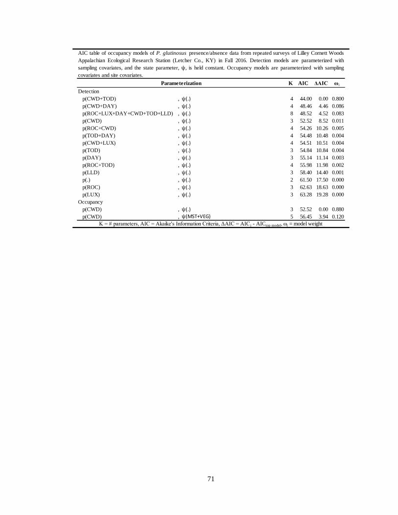
71

K AIC ΔAIC ω i

Detection

p(CWD+TOD) , ψ(.) 4 44.00 0.00 0.800

p(CWD+DAY) , ψ(.) 4 48.46 4.46 0.086

p(ROC+LUX+DAY+CWD+TOD+LLD) , ψ(.) 8 48.52 4.52 0.083

p(CWD) , ψ(.) 3 52.52 8.52 0.011

p(ROC+CWD) , ψ(.) 4 54.26 10.26 0.005

p(TOD+DAY) , ψ(.) 4 54.48 10.48 0.004

p(CWD+LUX) , ψ(.) 4 54.51 10.51 0.004

p(TOD) , ψ(.) 3 54.84 10.84 0.004

p(DAY) , ψ(.) 3 55.14 11.14 0.003

p(ROC+TOD) , ψ(.) 4 55.98 11.98 0.002

p(LLD) , ψ(.) 3 58.40 14.40 0.001

p(.) , ψ(.) 2 61.50 17.50 0.000

p(ROC) , ψ(.) 3 62.63 18.63 0.000

p(LUX) , ψ(.) 3 63.28 19.28 0.000

Occupancy

p(CWD) , ψ(.) 3 52.52 0.00 0.880

p(CWD) , ψ(MST+VEG) 5 56.45 3.94 0.120

AIC table of occupancy models of P. glutinosus presence/absence data from repeated surveys of Lilley Cornett Woods

Appalachian Ecological Research Station (Letcher Co., KY) in Fall 2016. Detection models are parameterized with

sampling covariates, and the state parameter, ψ, is held constant. Occupancy models are parameterized with sampling

covariates and site covariates.

Parameterization

K = # parameters, AIC = Akaike's Information Criteria, ΔAIC = AIC i - AICtop model, ωi = model weight

72

APPENDIX 7:

AIC table of conditional two-species occupancy models of P. richmondi and P. kentucki

co-occurrence in the old-growth forest of Lilley Cornett Woods Appalachian Ecological

Research Station (Letcher Co., KY) in Fall 2016

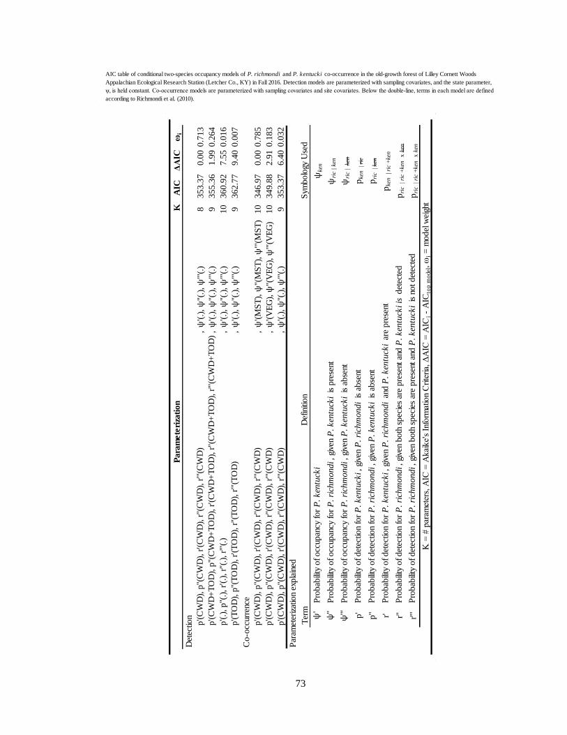
73

AIC table of conditional two-species occupancy models of P. richmondi and P. kentucki co-occurrence in the old-growth forest of Lilley Cornett Woods

Appalachian Ecological Research Station (Letcher Co., KY) in Fall 2016. Detection models are parameterized with sampling covariates, and the state parameter,

ψ, is held constant. Co-occurrence models are parameterized with sampling covariates and site covariates. Below the double-line, terms in each model are defined

according to Richmondi et al. (2010).

KA

ICΔAIC

ωi

Det

ectio

n

,ψ

'(.)

, ψ

''(.)

, ψ

'''(.

)8

353.3

70.0

00.7

13

,ψ

'(.)

, ψ

''(.)

, ψ

'''(.

)9

355.3

61.9

90.2

64

,ψ

'(.)

, ψ

''(.)

, ψ

'''(.

)10

360.9

27.5

50.0

16

,ψ

'(.)

, ψ

''(.)

, ψ

'''(.

)9

362.7

79.4

00.0

07

Co-o

ccur

renc

e

,ψ

'(M

ST

), ψ

''(M

ST

), ψ

'''(M

ST

)10

346.9

70.0

00.7

85

,ψ

'(V

EG

), ψ

''(V

EG

), ψ

'''(V

EG

)10

349.8

82.9

10.1

83

,ψ

'(.)

, ψ

''(.)

, ψ

'''(.

)9

353.3

76.4

00.0

32

Par

amet

eriz

atio

n ex

pla

ined

Ter

m

ψ'

ψ''

ψ''' p'

p'' r' r''

r'''

K = # parameters, AIC = Akaike's Information Criteria, ΔAIC = AIC

i - A

ICto

p m

ode

l, ω

i = m

odel

wei

ght

Para

mete

riza

tion

p'(C

WD

), p

''(C

WD

), r

'(C

WD

), r

''(C

WD

), r

'''(C

WD

)

p'(C

WD

), p

''(C

WD

), r

'(C

WD

), r

''(C

WD

), r

'''(C

WD

)

p'(C

WD

), p

''(C

WD

), r

'(C

WD

), r

''(C

WD

), r

'''(C

WD

)

p'(C

WD

), p

''(C

WD

), r

'(C

WD

), r

''(C

WD

), r

'''(C

WD

)

p'(C

WD

+T

OD

), p

''(C

WD

+T

OD

), r

'(C

WD

+T

OD

), r

''(C

WD

+T

OD

), r

'''(C

WD

+T

OD

)

p'(.)

, p''(

.), r'(.

), r

''(.)

, r'''(

.)

p'(T

OD

), p

''(T

OD

), r

'(T

OD

), r

''(T

OD

), r

'''(T

OD

)

Pro

bab

ility

of occ

upan

cy for

P. ken

tuck

i

Pro

bab

ility

of occ

upan

cy for

P. ri

chm

ondi,

giv

en P

. ken

tuck

i is

pre

sent

Def

initi

on

Sym

bolo

gy U

sed

Pro

bab

ility

of det

ectio

n fo

r P

. ri

chm

ondi,

giv

en b

oth

spec

ies

are

pre

sent

and

P. ken

tuck

i is

not det

ecte

d

ψke

n

ψri

c |

ken

ψri

c |

ken

pke

n |

ric

pri

c |

ken

pke

n |

ric

+ke

n

pri

c |

ric

+ke

n

x k

en

pri

c |

ric

+ke

n

x k

en

Pro

bab

ility

of occ

upan

cy for

P. ri

chm

ondi,

giv

en P

. ken

tuck

i is

abse

nt

Pro

bab

ility

of det

ectio

n fo

r P

. ken

tuck

i, g

iven

P. ri

chm

ondi

is a

bse

nt

Pro

bab

ility

of det

ectio

n fo

r P

. ri

chm

ondi,

giv

en P

. ken

tuck

i is

abse

nt

Pro

bab

ility

of det

ectio

n fo

r P

. ken

tuck

i, g

iven

P. ri

chm

ondi

and P

. ken

tuck

i ar

e pre

sent

Pro

bab

ility

of det

ectio

n fo

r P

. ri

chm

ondi,

giv

en b

oth

spec

ies

are

pre

sent

and

P. ken

tuck

i is

det

ecte

d