national bank of belgium - nbb.be · national bank of belgium ... describes the behaviour of firms...
TRANSCRIPT

NBB WORKING PAPER No. 24 - MAY 2002 1
NATIONAL BANK OF BELGIUM
WORKING PAPERS - RESEARCH SERIES
THE IMPACT OF UNCERTAINTY ON INVESTMENT PLANS
_______________________________
Paul Butzen(*)
Catherine Fuss (**)
Philip Vermeulen(***)
The views expressed in this paper are those of the authors and do not necessarilyreflect the views of the National Bank of Belgium, nor of the European Central Bank
(*) National Bank of Belgium, Research Department, (e-mail: [email protected]).(**) National Bank of Belgium, Research Department, (e-mail: [email protected]).(***) European Central Bank, (e-mail: [email protected]).

2 NBB WORKING PAPER No. 24 - MAY 2002
Editorial Director
Jan Smets, Member of the Board of Directors of the National Bank of Belgium
Statement of purpose:
The purpose of these working papers is to promote the circulation of research results (Research Series) and analyticalstudies (Documents Series) made within the National Bank of Belgium or presented by outside economists in seminars,conferences and colloquia organised by the Bank. The aim is thereby to provide a platform for discussion. The opinionsare strictly those of the authors and do not necessarily reflect the views of the National Bank of Belgium.
The Working Papers are available on the website of the Bank:http://www.nbb.be
Individual copies are also available on request to:NATIONAL BANK OF BELGIUMDocumentation Serviceboulevard de Berlaimont 14B - 1000 Brussels
Imprint: Responsibility according to the Belgian law: Jean Hilgers, Member of the Board of Directors, National Bank of Belgium.Copyright © National Bank of BelgiumReproduction for educational and non-commercial purposes is permitted provided that the source is acknowledged.ISSN: 1375-680X

NBB WORKING PAPER No. 24 - MAY 2002 1
Abstract
In this paper we investigate how demand and output price uncertainty affect investment
plans of Belgian manufacturing firms. We obtain time-varying uncertainty measures at the
firm and industry level from the Belgian monthly business cycle survey and investment
plans from the half-yearly investment survey. Using investment plans instead of realised
investment data, e.g. annual accounts data, is, from an informative point of view, superior
since it is more likely to reveal the features of the decision formation process and,
therefore, it is most closely related to economic theory. Business investment is normally
planned well in advance, because it involves time and costs to implement, and theory
describes the behaviour of firms at the moment of their decision, which can be assumed to
be fully captured in survey data. In order to find robust predictions we estimate three
different specifications, each of which can be considered as a benchmark in the literature:
two reduced form equations and a structural Euler equation. Our results show that
uncertainty depresses investment. These results hold for industry- as well as for firm-
specific demand uncertainty. Moreover, referring to Euler equation, uncertainty postpones
investment today in favour of investment tomorrow. This effect is stronger for firms with
more irreversible investment. Hence, our results seem to confirm to predictions of the real
option theory.
Keywords: investment, uncertainty, irreversibility, real options, survey data
JEL Classification: D92, E22, D82, C23.
Editorial
On May 27-28, 2002 the National Bank of Belgium hosted a Conference on "Newviews on firms' investment and finance decisions". Papers presented at thisconference are made available to a broader audience in the NBB Working Papersno 21 to 33.

2 NBB WORKING PAPER No. 24 - MAY 2002

NBB WORKING PAPER No. 24 - MAY 2002 1
TABLE OF CONTENTS
1. INTRODUCTION........................................................................................................... 1
2. THE INVESTMENT-UNCERTAINTY NEXUS IN THE LITERATURE......................... 3
2.1. Theoretical reflections ................................................................................................... 3
2.2. Empirical methodology.................................................................................................. 4
2.3. Measuring uncertainty................................................................................................... 5
3. DESCRIPTION OF THE DATA..................................................................................... 7
4. THE EMPIRICAL MODEL .......................................................................................... 10
5. THE RESULTS ........................................................................................................... 13
5.1. Reduced form specifications ...................................................................................... 13
5.2. Euler equation............................................................................................................. 17
6. CONCLUSIONS.......................................................................................................... 22
References ........................................................................................................................... 24

2 NBB WORKING PAPER No. 24 - MAY 2002

NBB WORKING PAPER No. 24 - MAY 2002 1
1. INTRODUCTION
In this paper, we investigate how demand and output price uncertainty affect the investment
behaviour of a panel of Belgian manufacturing firms. A number of studies have recently analysed
the investment behaviour of Belgian manufacturing firms using accounting data1. Only three studies
(Cassimon et al, 2002, Gérard and Verschueren, 2002, and Peeters, 2001), however, investigate the
effect of uncertainty on investment for Belgian manufacturing firms. Peeters (2001) estimates an
Euler equation augmented with uncertainty. She finds that output price uncertainty depresses
investment, but she detects no effects of demand uncertainty. Gérard and Verschueren (2002) use
both an Euler equation and a reduced form framework. Their results show little empirical support
for the role of investment price uncertainty. Cassimon et al (2002), on the contrary, obtain that
uncertainty with respect to profitability has an impact on the decision to invest. When investment is
irreversible, uncertainty also reduces the amount invested.
To reveal the role of uncertainty in the investment decision process, the amount of the
investment planned, rather than the actual amount of investment is the relevant variable. Investment
is usually planned well in advance, because it involves time and costs to implement. Since firms
take into account all available information and the uncertainty surrounding this information at the
moment of their decision, all information should be measured as closely as possible to that moment.
Hence, planned investment is, from an informative point of view, superior to actual investment, and
is most closely related to economic theory. Therefore, we use investment survey data in which
managers reveal their planned investment expenditures. We are aware of only two other research
papers that make use of planned investment data in order to investigate the effect of uncertainty on
investment (Guiso and Parigi, 1999, and Patillo, 1998). All other studies, instead, analyse realised
data, i.e. firm-level actual investment from annual accounts.
We further employ the business cycle survey conducted every month by the National Bank of
Belgium (NBB), to construct measures of demand and price uncertainty at the industry and firm
level. Our uncertainty measures are at the same time industry- or firm-specific, time-varying and
forward-looking; further they are derived from directly observable firms' expectations rather than
being based on an assumption about the firms' expectation formation model. We relate planned
investment to its neoclassical fundamentals, uncertainty and financial constraints measures.
Fundamentals and cash flow, which is commonly considered as a proxy for financial constraints,
are constructed from annual accounts.
1 Barran and Peeters (1998), Bond et al. (1997), Butzen et al (2001), Cassimon et al (2002), Deloof (1998),
Gérard and Verschueren (2002), Peeters (2001), Vermeulen (1998) and other papers presented at thisconference.

2 NBB WORKING PAPER No. 24 - MAY 2002
In order to find robust predictions we estimate three different specifications, each of which can
be considered as a benchmark in the literature. First, we estimate an error correction model
augmented with uncertainty, as in Bloom et al. (2001). Second, we apply a variant of the
specification used in Guiso and Parigi (1999). Third, for comparability with the existing evidence
on Belgian firms, we estimate an Euler equation as in Gérard and Verschueren (2002) and Peeters
(2001).
These regressions allow us to test the predictions of what has become in the last decade one of
the major strands in the investment literature: the real options theory. According to this theory,
when investment is irreversible, i.e. investment is a sunk cost, and if there exists some time
flexibility to postpone investment, firms might optimally wait to invest until more is know. So the
main conclusion of real option theory is that uncertainty depresses current irreversible investment
and postpones investment projects. Although all specifications we estimate, contain dynamics,
primarily, the investment Euler equation, which explicitly explains the intertemporal substitution of
investment expenditures, can verify this hypothesis. The real option literature yields more
ambiguous predictions with respect to the impact of uncertainty on the optimal amount of
investment and on the long-run capital stock. Several papers have indicated that the production and
market environment in which the firm operates matters and that a slightly different mix of various
parameters can substantially alter the conclusions (Bertola, 1988, Caballero, 1991, Pindyck, 1993,
and Abel et al, 1996). The total picture is even further blurred when one takes into account the
findings of an older strand of research (Hartman, 1972, and Abel, 1983), according to which
increased uncertainty will stimulate investment. Therefore, the sign of the long-run relationship
between uncertainty and investment needs to be determined on empirical grounds. All three
specifications can help to shed some light on this aspect.
This paper is organised as follows. Section 2 gives a brief overview of the prevailing
theoretical reflections and empirical approaches to the investment-uncertainty relationship. Section
3 describes our data. Here, we put emphasis on our contribution using survey data and how we
construct our uncertainty measures. The various model specifications are presented in Section 4 and
our empirical findings in Section 5. Section 6 summarises our main conclusions.

NBB WORKING PAPER No. 24 - MAY 2002 3
2. THE INVESTMENT-UNCERTAINTY NEXUS IN THE LITERATURE
2.1. Theoretical reflections
The seminal book of Dixit and Pindyck (1994) and the recent survey by Carruth et al (2000)
have summarised the renewed attention in the literature for the analysis of firms' behaviour under
uncertainty when investment expenditures are irreversible. Their key insight is that, under
irreversibility, there exists an option to postpone investment in order to obtain further information
about future market conditions. This option to wait has a value (the opportunity cost of investing
today) and, subsequently, firms will only invest when the net present value of the investment project
covers also this value. Therefore, irreversibility increases the hurdle that triggers investment
compared to the reversibility case (the irreversibility effect), and, moreover, this hurdle increases
with uncertainty (the uncertainty effect). So, real option theory predicts that uncertainty and
irreversibility depress current investment and delay investment projects. In linking option pricing
theory to investment behaviour the contribution of the real option hypothesis primary brings
insights into the timing of investment (e.g. the model of Mc Donald and Siegel, 1986).
Real option theory is less conclusive with respect to the optimal amount of investment and
long-run capital stock. Several papers have shown that the sign and the magnitude of the effect of
uncertainty on the optimal investment policy rule depends on the precise mix of characteristics such
as the degree of irreversibility, the competitiveness of product markets, the production process
(substitutability, returns to scale) and manager's attitude towards risk (Bertola, 1988, Caballero,
1991, Pindyck, 1993, and Abel et al, 1996). Moreover, Abel and Eberly (1999) prove that one
should add to this ambiguity a so-called 'hangover' effect, i.e. the discrepancy between the firm's
current capital stock, which reflects the firm's optimal behaviour to favourable circumstances in the
past, and the lower level that it optimally would like to hold due to the occurrence of a slacking
demand, but is unable to reach because of the irreversibility constraint. The 'hangover' effect makes
current investment function of past events, and so, it introduces hysteresis.
The total picture becomes even further confused when one takes into account the findings of an
older strand of research (Hartman, 1972, and Abel, 1983), which neglects the role of irreversibility.
According to this theory increased uncertainty will stimulate investment of a risk-neutral,
competitive firm with a constant returns to scale production process. Under these features the
marginal product of capital is a convex function in the variables whose evolution is uncertain. In
that case, Jensen's inequality applies: a higher, but mean-preserving, volatility, increases the optimal
capital stock. To sum up, there exists no theoretical consensus regarding the long-run investment-
4 NBB WORKING PAPER No. 24 - MAY 2002
uncertainty nexus. Hence, the sign of this relationship needs to be determined on empirical grounds.
On the contrary, it is acknowledged that irreversibility and uncertainty affect the timing of
investment by delaying investment.
2.2. Empirical methodology
There are several complications involved with the empirical investigation of the investment-
uncertainty relationship. Neither is there consensus on the most suitable measure to proxy
uncertainty (see next section), nor on the empirical specification.
Following the theoretical ambiguity of the long-run investment-uncertainty rela tionship, as
described in the previous section, a majority of studies have tried to settle it empirically2. In our
paper we will not only assess this feature but also the other prominent feature of the real option
hypothesis: i.e. irreversibility and uncertainty affect the timing of investment. The existence of
threshold effects above which investment is triggered and below which the option to delay is
exercised has implications for the dynamics of investment resulting in periods of inaction.
Irreversibility will change, at least at the project-level, the investment behaviour of firms from being
smooth and continuous (the reversibility case) to one that is lumpy and frequently zero.
Several empirical papers have focused on this aspect of real option models. One approach,
which deals with the short run dynamics, tries to identify the factors, which affect the trigger values
of investment (Pindyck and Solimano, 1993, Patillo, 1998, Cassimon et al, 2002). This method,
however, has a number of drawbacks. First, one needs to impose a considerable amount of structure
(a particular production technology, competitive markets, etc.) in order to calculate the marginal
revenue product of capital (MRPK), which needs to be compared to the marginal cost of capital
adjusted for uncertainty. Second and more importantly, the value that triggers investment is not
directly observable. Commonly, one has to assume that the theory is correct and that firms with a
positive investment rate have just hit the trigger. Under this assumption, one can take the measured
MRPK as a proxy for the unobserved trigger. Of course, the condition that the MRPK will never
rise above the trigger, is rather severe and will not always hold empirically. Finally, although
lumpy and zero investment behaviour has been observed with plant-level data (Doms and Dunne,
1998), aggregation, even at the firm-level, across multiple investment decisions (project, plants)
will smooth away much of the lumpiness. In our data set, the frequency of zero investment is much
2 Among many others are Bloom et al (2001), Driver and Moreton (1992), Driver et al. (1996), Ferderer
(1993a, b), Ghosal and Lougani (2000), Guiso and Parigi (1999), Meersman and Cassimon (1995),Peeters (2001), Patillo (1998), Price (1995), von Kalckreuth (2000).

NBB WORKING PAPER No. 24 - MAY 2002 5
lower for large firms (1%) than for small firms (7.4%), consistently with the fact that aggregation
across plants and projects smoothes investment.
Therefore, other approaches put less emphasis on the rare zero investment observations and
incorporate some weaker form of lumpy dynamics. They introduce non-quadratic adjustment costs
where the relationship between investment and its fundamentals becomes non-linear (Abel and
Eberly, 1994, and Eberly, 1997). Still other papers follow a more ad hoc approach and specify a
traditional error correction model (ECM) to capture the dynamics (Price, 1995, and Bloom et al,
2001). The advantage of this model is that it can capture a wide variety of relatively complex
adjustment processes. On the other hand, as for every reduced form approach, the Lucas critique
applies.
In our paper we specify not only a reduced form ECM, but we also estimate an Euler type of
equation. Directly derived from the first order conditions of a dynamic optimisation problem, the
Euler equation most naturally embodies the intertemporal nature of the investment decision. It
offers the advantage that deep structural parameter can be obtained. The disadvantage is that one
needs to put some structure on the model (choice of production and adjustment cost technology),
which makes the results conditional upon this structure.
2.3. Measuring uncertainty
Investment depends on the expected future returns and the uncertainty surrounding these
expectations. The stochastic processes of the underlying variables determine expectations about
future returns. We concentrate our analysis on demand and output price uncertainty, because we
have firm-subjective expectations of these variables. Further, we believe that macroeconomic
variables may be less relevant than firm-specific factors as they can explain only time series
variations and not cross-firms variations.
Data on firm-specific uncertainty are rarely readily available. To our knowledge, within the
field of business investment research only two papers (Guiso and Parigi, 1999, and Patillo, 1998)
refer to such directly available measures of firm-specific uncertainty. Both papers obtain a measure
for demand uncertainty from a single survey, which reports the entrepreneur's subjective probability
distribution of expected future demand. Most other papers construct a proxy for uncertainty based
on the volatility of some variable or on the variance of errors of some forecasting model3.
Uncertainty measured in this way is based on a parametric assumption about the firms' process of

6 NBB WORKING PAPER No. 24 - MAY 2002
expectations formation. This implies that one assumes, first, that the econometrician knows the true
model of expectations formation, and, second, that all firms have the same model.
On the contrary, we construct our measure of uncertainty from observed firms' expectations, a
strategy that few papers have followed. When firms' subjective expectations are available, one can
construct both aggregate and firm-specific measures of uncertainty. This is the approach we follow.
Since future forecasts which are reported in surveys, are often strictly qualitative in nature, they
need a special treatment to generate quantitative measures. In the literature, several methods have
been suggested to construct measures of aggregate or industry-level uncertainty from individual
answers4. The intuition behind all these measures is that they are larger as more respondents
disagree about the future. We use the monthly business survey, conducted by the National Bank of
Belgium, which reports qualitative information on firm's expected demand growth and on firm's
expected price growth. We measure uncertainty by the disconformity of expectations across firms
and across the twelve months of the year.
3 See, among others, Bulan (2000), Gérard and Verschueren (2002), Ghosal and Lougani (2000), Meersman
and Cassimon (1997), Peeters (2001), Price (1995), von Kalckreuth (2000).4 For instance, Theil (1952), Caselli et al (2000), Carlson and Parkin (1975), Driver and Moreton (1992).

NBB WORKING PAPER No. 24 - MAY 2002 7
3. DESCRIPTION OF THE DATA
In order to test the theoretical hypotheses, we match three different data sets. The NBB
investment survey provides us with data about planned investment. The NBB annual accounts
database is used to construct the required firm-specific control variables such as the capital stock,
sales, cash flow, etc. The NBB business survey is used to construct sector-specific and firm-specific
measures of demand and output price uncertainty.
The NBB investment survey is conducted twice a year, once during the month of May (Spring
Survey) and once during the month of November (Autumn survey). Since the mid eighties the
questionnaire did not change and the results are comparable from 1986 onwards. The survey
provides quantitative information (i.e. in euros) about the firm's investment expenditures in the
previous year, the plans for the current year, and the firm's investment plans for the next year. The
questionnaire explicitly states that the firm is only presumed to provide a value for investment
planned when a sure decision in this respect has been made. From 1986 to 2001 in total 2515 firms
of 22 different industries have participated in this survey for one or several years, and they did so
rather seriously 5. We estimate our investment regressions using both the Autumn and Spring
surveys. First, we use firm’s planned investment for the year t+1 from the Autumn survey
conducted in year t. Second, we use the firm’s planned investment for the year t+1 from the Spring
survey in year t+1 (both are denoted IPit+1). In the second case, part of the planned investment is
therefore already realised. Realised investment over the previous year is also revealed in the survey.
Annual accounting data of Belgian firms are collected by the National Bank of Belgium6. They
are used to construct a number of control variables, which, according to theory, should appear in our
analysis. First, the real capital stock is obtained as the book accounting value of the capital stock,
deflated by the industry investment price index7 corrected for the average age (using the formulae as
in Bond et al, 1997, or Chatelain et Teurlai, 2000). Sales are proxied by value added, due to data
5 The actual investment of the previous year reported in the Spring survey coincided with the annual
accounts data nearly perfectly for 85% of the firms.6 Almost every non-financial firm reports annual accounts, by legal obligation. All accounts are submitted
to substantial accounting and logical consistency controls, and, if necessary, corrections are made. Thedata therefore satisfy the highest quality standards.
7 Firm-specific investment prices are not available. We use 2-digit NACE codes for investment and value-added prices. The construction of the capital stock is explained in the appendix.

8 NBB WORKING PAPER No. 24 - MAY 2002
availability8. Cash flow is defined as net profits plus depreciation9. The wage sum is directly
reported in the annual accounts.
The NBB business survey is used to construct measures of uncertainty and expected future
sales growth. This monthly survey reports qualitative information about the firm's demand and price
conditions. We focus on the answers to the following question: “For the next three months, the
demand of your customers for this product, will according to you be: (a) stronger, (b) unchanged,
(c) weaker, than is usual in the period of the year.” The term usual includes normal seasonal
fluctuations, and therefore the question really asks for changes relative to “normal business”. A
similar question is asked for prices. This survey allows us to construct a measure of uncertainty,
which is at the same time forward-looking, firm- (or sector-) specific and time varying, and not
based on a priori assumption about the firm's expectation formation process. Rather, the measure is
based on firm's subjective expectations about future demand and price conditions. We proxy
uncertainty by Theil (1952) 's disconformity index, i.e.: σt = [(%up+%down) - (%up-%down)²], with %up
and %down, the percentage of observations of expectations of positive growth and negative growth,
respectively. The index ranges from 0 to 1. When the answers are all identical, the index is equal to
zero. The higher the disconformity index, the more different the answers during the year. The
sector-specific index, σst, is based on the percentage over all months of the year and all firms of the
same industry10. The firm-specific uncertainty index, σit, is constructed by computing the
percentage over the 12 surveys of the year11.
We also use this survey to construct a measure of observed firm's subjective expectations of
future demand growth, Et(∆yit+1), which appears in the ECM as well as in the Guiso and Parigi
(1999) specification. This is simply equal to (%up-%down). This gives an index of the direction of
demand expectations. The index ranges from -1 to 1; if the index is 1. The firm has expected all
12 months a stronger demand than usual, if the index is –1 the firm has expected weaker demand for
12 months. This allows us to take into our analysis firm's subjective expectation about future market
8 Small firms do not provide as detailed information as large firms do, and among other things do not have
to report sales. A company is regarded as "large", in 1999. either when the yearly average of its workforceis at least 100 or when at least two of the following thresholds were exceeded: (1) yearly average ofworkforce: 50. (2) turnover (excluding VAT) : EUR 6.250.000. (3) balance sheet total : EUR 3.125.000. Ingeneral, the values of the latter two thresholds are altered every four years in order to take account ofinflation.
9 Again the definition differs for small and large firms according to data availability.10 In order to match the business survey with the investment survey, and in order to guarantee a sufficiently
large number of firms per sector, we focus on seven (aggregated) sectors: food, textiles, wood, paper,chemicals, non-metal and metal.
11 Not all firms answer to each survey, but restricting to firms that have answered all 12 months leads to amuch more precise and reliable measure of the uncertainty index.

NBB WORKING PAPER No. 24 - MAY 2002 9
conditions. We additionally compare the results including this measure with those based on a
rational expectations hypothesis.
We do not have at our disposal a first best data set, i.e. a data set containing a direct measure of
the entrepreneur's subjective probability distribution of expected future demand, as in Guiso and
Parigi (1999), and Patillo (1998), but we are still able to construct uncertainty measures using the
firm's subjective expectations on future demand (or output prices). This procedure, at least, is
second best, since it releases us from postulating an implicit process for the formation of
expectations (e.g. as in Gérard and Verschueren, 2002, Ghosal and Lougani, 2000, Peeters, 2001, or
von Kalckreuth, 2000) and, moreover, provides us with a forward-looking measure. Furthermore,
since the business survey is conducted on a higher frequency than the investment survey (monthly
versus half-yearly), the final uncertainty measure can be at the same time firm (or sector) specific
and time-varying. Of course, there are some caveats. First, quantifying information contained in a
qualitative survey is never an easy and exempt-of-error task (see for example the analysis of
Batchelor, 1986). Second, there is a time-horizon mismatch between the questions in both surveys.
The investment survey asks for the firm's investment intentions for the next year, whereas in the
business survey firms have to reveal their demand and output price prospects for the coming three
months.
The data appendix gives extensive information about the precise definition of the variables and
the trimming procedure, and also provides some descriptive statistics of our sample and its
representativity.

10 NBB WORKING PAPER No. 24 - MAY 2002
4. THE EMPIRICAL MODEL
We attempt to obtain rather robust conclusions on the effect of uncertainty on investment.
Therefore, we estimate three different specifications, which can be considered being the benchmark
in the current empirical investment literature. The first two specifications are in reduced form, so
they are not explicitly derived from a particular optimising behaviour of a firm, but rather they
represent an empirical approximation to some complex underlying process that generates the data.
The justification behind these specifications is that, starting from a formal intertemporal
optimisation problem of a representative firm and taking into account elements of irreversibility
and/or adjustment costs, results in closed-form solutions that are highly non-linear and often
unmanageable without making some simple linear approximation. With this approach we actually
follow the procedure adopted by many authors, who prefer to treat the item of irreversible
investment, in a more pragmatic way.
Because we use reduced-form equations, we try different specifications as a robustness check.
The firm plans its investment in the next period if it expects good opportunities (sales growth) and it
expects to collect the necessary financing funds (internally or externally)12. If adjustment to the
optimal capital stock is not immediate, it may consider current values of the above variable, realised
investment and deviations from its long-run equilibrium. Finally, uncertainty about the future may
lead the firm to postpone investment decisions until new information is available, this would imply
lower investment plans which may be revised upwards in case of good news in the next period13.
The first specification is an accelerator model, which controls for demand by entering sales
growth (∆yit) as in von Kalckreuth (2000) 14. We also include an error correction term and assume,
as in Bloom et al (2001), that in the long-run, the capital output-ratio is constant, so that deviations
from the long-run equilibrium simplify to (kit-1- yit-1)15. We also include expectations on future
market conditions in the equation. However, future sales growth partly captures future cash flow.
12 We use fixed effects and time dummies. These variables can, among other things, be seen as a proxy for
the user cost of capital. Since the user cost of capital is not the focus of our paper, we do not think thatthis strategy would be harmful to the results.
13 Bloom et al (2001) have argued that uncertainty may also reduce the sensitivity of the firm to salesgrowth. We tested for such effect but it turned out to be non-significant.
14 von Kalckreuth enters multiple lags of sales growth. We prefer to enter the lagged investment ratiotogether with one lag of sales growth, which implicitly is like entering an infinite number of lags of salesgrowth with restrictions on the coefficients of these lags. The advantage of this parsimoniousspecification is that less observations are lost due to constructing lagged variables.
15 Preliminary analysis shows that imposing this restriction substantially improves the results, in terms ofboth specification and significance of the coefficients. It also prevents from obtaining aberrant values forthe returns to scale parameter, as so often is seen in the literature. So, imposing this restriction reflectscurrent best practices. Moreover, it enhances comparability with the Euler specification, in which thisassumption is made in order to calculate the MRPK.

NBB WORKING PAPER No. 24 - MAY 2002 11
Thereby to avoid multicollinearity problems, we do not include future cash flow together with
future sales growth, current sales growth and cash flow (CFit/Kit). Finally, time dummies (δt)
capture macroeconomic fluctuations. Small cases represent logs. Our first specification is then
(1) IPit+1/Kit = δt + α Iit/Kit-1 + γ.Et(∆yit+1) + β.∆yit + ϕ.CFit /Kit + θ.σst -λ.(kit-1-yit-1) + εit+1
with σst representing industry-specific demand or output price uncertainty (whereby the subscript s
is replaced by i when firm-specific uncertainty is used).
The second specification controls for demand by including the current value added capital ratio
(Yit/Kit) rather than current sales growth. By doing, one obtains a similar specification as in Guiso
and Parigi (1999). The major difference with the first specification is the omission of the error
correction term :
(2) IPit+1/Kit = δt + α Iit/Kit-1 + γ.Et(∆yit+1) + β. Yit /Kit + ϕ.CFit /Kit + θ.σst + εit+1
The third specification is the classical Euler equation. This equation, in particular, allows us to
investigate the intertemporal properties of the investment decision process, since it examines the
choice between investing today or tomorrow. Hence, this specification is most interesting to test the
real option theory, which prominent feature refers to the timing of investment. A complete
derivation of the Euler equation can be found in the Appendix. Our Euler equation becomes (with
Fit representing the production function, witLit the wage sum, βt+1 the discount rate, δi the
depreciation rate and the pI 's the investment price):
(3)
]p/)p(E)1)(1(12
[1
*)K
L
p
w(
1)
K
F
p
p(
)1
1()K/I(
2
1)K/I()Kp/Ip(E)1(
It
I1tit1iti
2
stit
itIit
it
it
itIt
it2itititit1it
It1it
I1tt1iti
++
++++
βδ−−αφ+αφ−+αφα
+
+σαθ+
α+
αε
−−=+−βδ−
The adjustment cost parameter is α and ε represents the absolute value of the price elasticity of
the firm's output demand. Under monopolistic competition, one expects for the latter parameter a
value close to, but greater than one. An important feature of the data is that we can replace expected
investment, Et(pIt+1 Iit+1), with the observed investment plans of the survey, pI
t+1 IPit+1. So, we do not
need to make an explicit assumption with respect to the firm's expectations formation process. Most

12 NBB WORKING PAPER No. 24 - MAY 2002
studies assume rational expectations and replace expected values by realised ones. This practice
introduces a forecast error in the equation and makes regressors correlated with the error term.
Note that the interpretation of the coefficient on uncertainty for the Euler equation is different
from the interpretation for the reduced form regressions. The reduced form regressions estimate the
effect of uncertainty during year t on the investment planned for year t+1 (where the planning
happens in Autumn of year t or Spring in year t+1), conditional on year t investment. The Euler
equation describes the effect of uncertainty on the intertemporal substitution between actual
investment in year t and planned investment for the year t+1. Uncertainty will have a negative effect
on the level of investment in year t when the coefficient on uncertainty is positive (note that I/Kt
enters on the left hand side with a negative sign), but also, by forward substitution, on investment
rates in the future. Only, a positive coefficient for uncertainty, in addition, implies a shift of
investment from year t to year t+1. Hence, the negative effect of future investment will be tempered
compared to current investment.

NBB WORKING PAPER No. 24 - MAY 2002 13
5. THE RESULTS
5.1. Reduced form specifications
We first present our estimates of the reduced-form equations (1) and (2). In this section, we use
investment plans as reported in the Autumn survey. Some robustness checks with respect to the
Spring survey are reported in appendix B. We assume that all variables in period t are
predetermined. We believe that our uncertainty measure is truly exogenous for the plans made
during t for year t+1. Clearly, it would be hard to find a reason why e.g. increased demand expected
in August year t for Sept-Nov year t could be influenced by the planned investment for year t+1. We
assume therefore that the direction of causation can only go from uncertainty to investment plans
and not the other way around. We also use the firm-specific measure for future growth described in
the above section, and assume for the same reason that it is predetermined.
Estimating both reduced form equations, several assumptions can be made, which determine
the use of a particular estimator. Assuming no fixed effects and using our measure of future sales
growth, equation (1) can be consistently estimated by OLS. Otherwise, there exist two endogeneity
problems. The first is related to the inclusion of fixed effects. These effects capture various
unobserved firm-specific factors such as the firm-specific component of the user cost, productivity
growth, depreciation rate, etc. The model must then be transformed to get rid of the fixed effects
and instrumented because the transformation (e.g. within or first differences are often used) creates
a correlation between the transformed error term and the transformed regressors. The second
endogeneity problem is related to proxying expected future sales growth by its realisation, i.e.
assuming that firms are rational in forming their expectations. This practice, however, introduces a
forecast error in the equation and, in this case, the model also needs to be estimated by some
instrumental variable technique. We include all variables of the equation in t and t-1 in the
instrument set.
We compare our results using sector-specific and firm-specific uncertainty. Assessing the
effect of industry-specific uncertainty on investment behaviour, leaves us with a fairly large amount
of the degrees of freedom which allows us to include an adequate dynamical path. In this case, we
allow for fixed effects and estimate equation (1) with Arellano and Bond (1991) first difference
GMM estimator. Although we control for a number of firm-specific variables (such as sales and
cash-flow), the fact that we consider sector-specific uncertainty rather than firm-specific uncertainty
may introduce the firm-specific component of uncertainty in the error term, calling for a fixed effect

14 NBB WORKING PAPER No. 24 - MAY 2002
estimation16. We investigate below whether the results change when taking into account firm-
specific uncertainty.
Table 1 below reports the first difference Arellano-Bond GMM estimates of equation (1) with
sector-specific uncertainty. We compare a purely backward-looking specification, without future
sales growth, with two forward-looking specifications. In the first, we assume rational expectations.
In the second, we used our sector-specific proxy of observed expectations for future sales growth,
Et(∆yit+1). The model is correctly estimated, as evidenced by the Sargan, m1 ad m2 statistics.
The results show that firms smooth investment (the coefficient on realised investment is
significantly positive and around 0.09). This may be due to the fact that investment is aggregated
over projects and plants, and that investment projects may run over several years.
Including expected future sales growth, there is evidence of accelerator effects. In the rational
expectation specification, future sales growth and current sales growth are both significant.
However, in the case of observed expectations with demand uncertainty, future sales growth is
significant at the 16% level only and current sales growth becomes insignificant. This may indicate
that our proxy for observed expectations is poor, which may be due to the fact that it is based on
qualitative information with a short forecast horizon (3-months) or to the fact that it is sector-
specific. Estimates with firm-specific observed expectations, discussed below, also show that this
variable is not significant. Using a similar proxy based on three-month forecast horizon, Houbedine
(2001) also finds no effect of future growth on investment plans. On the contrary, using a measure
of one-year ahead expected future growth, Patillo (1998) finds that this variable has a significant
effect on (positive) investment. This suggests that, because of a short-time horizon, our proxy of
observed expectations is a poor indicator of the true firm's expectations of next year growth, and
that the latter may be better proxied assuming rational expectation.
The coefficient on cash flow is never significant. This may be due to the fact that the
interpretation of cash flow is ambiguous; it has been interpreted as evidence of financial constraints,
but may also proxy for future sales growth opportunities (see, for example, the discussion in Kaplan
and Zingales, 1997).
The error correction term is significant and correctly signed. This indicates at the same time
that firms adjust their investment plans to deviations of their capital stock from long-run
16 Indeed, preliminary estimates (available on request) show that the omission of fixed effects generates very
poor results and lead to misspecification problems.

NBB WORKING PAPER No. 24 - MAY 2002 15
equilibrium, and that there are long-run constant returns to scale. The value of the adjustment
parameter, between 0.06 and 0.08 suggests a slow speed of adjustment towards long-run
equilibrium, as is generally found in the literature.
Finally, although price uncertainty is never significant, demand uncertainty is significantly
negative across all three specifications. The coefficient of demand uncertainty lies between -0.15
and -0.16. This implies that a one standard deviation increase in sector demand uncertainty (i.e.
0.05) reduces the rate of investment plans by 3% of its mean. Although non-negligible, the effect is
not very large, as has been found elsewhere in the literature.
Table 1: GMM estimation in first difference with fixed effects and sector-specificuncertainty
demand uncertainty price uncertainty
coeff t-stat coeff t-stat coeff t-stat coeff t-stat coeff t-stat coeff t-statIit/Kit-1 0.09 2.41 0.09 2.38 0.08 2.20 0.09 2.46 0.09 2.40 0.09 2.36
Et(∆yst+1) 0.08 1.41 0.12 2.14
∆yit+1 0.07 1.62 0.09 1.91
∆yit 0.03 0.75 0.07 1.51 0.03 0.79 0.03 0.84 0.09 1.74 0.03 0.78
CFit/Kit-1 0.01 0.38 0.01 0.50 0.01 0.27 0.01 0.31 0.01 0.44 0.01 0.48
σDst -0.15 -2.21 -0.15 -2.30 -0.16 -2.29
σPst -0.03 -0.27 -0.02 -0.15 0.04 0.37
kit-1-yit-1 -0.07 -2.36 -0.08 -2.62 -0.06 -2.33 -0.07 -2.29 -0.08 -2.61 -0.06 -2.11
# obs – firms 1303 256 1303 256 1303 256 1303 256 1303 256 1303 256Sargan-p-value 378.48 0.07 375.81 0.08 454.22 0.06 360.91 0.21 356.72 0.24 445.25 0.10m1 - p-value -6.59 0.00 -6.68 0.00 -6.58 0.00 -6.52 0.00 -6.62 0.00 -6.56 0.00m2 - p-value 0.55 0.58 0.60 0.55 0.64 0.52 0.53 0.60 0.55 0.58 0.69 0.49
Instrument set: lags of Iit/Kit-1 ,Iit-1/Kit-2 ,yit, yit-1 ,CFit/Kit-1 ,CFit-1/Kit-2 ,σst, σst-1 ,σst-2 ,kit, ,kit-1 ,Et(∆yst+1),Et-1(∆yst), Et-2(∆yst-1),All regressions include time dummies, first step robust results
We now investigate the effect of firm-specific demand uncertainty on investment plans. The
requirement to obtain a meaningful measure of firm-specific uncertainty, i.e. we restrict ourselves to
firms that answered the question regarding their demand prospects every single month, reduces
severely the number of firms. We have 473 firm-observations on 249 firms after removing outliers.
The data set is unbalanced with most firms having only 1 or very few observations, i.e. with an
average of 1.9 observations per firm. Given the size of the sample the best strategy is to stick to
OLS estimates rather than using methods which require a larger number of observations, but to
include controlling variables to reduce the potential importance of potential firm-specific effects
and diminish the potential correlation of uncertainty with the firm specific effect. Among others, the
inclusion of firm specific uncertainty, rather than sector specific uncertainty, should diminishes
potential fixed effects problems.
16 NBB WORKING PAPER No. 24 - MAY 2002
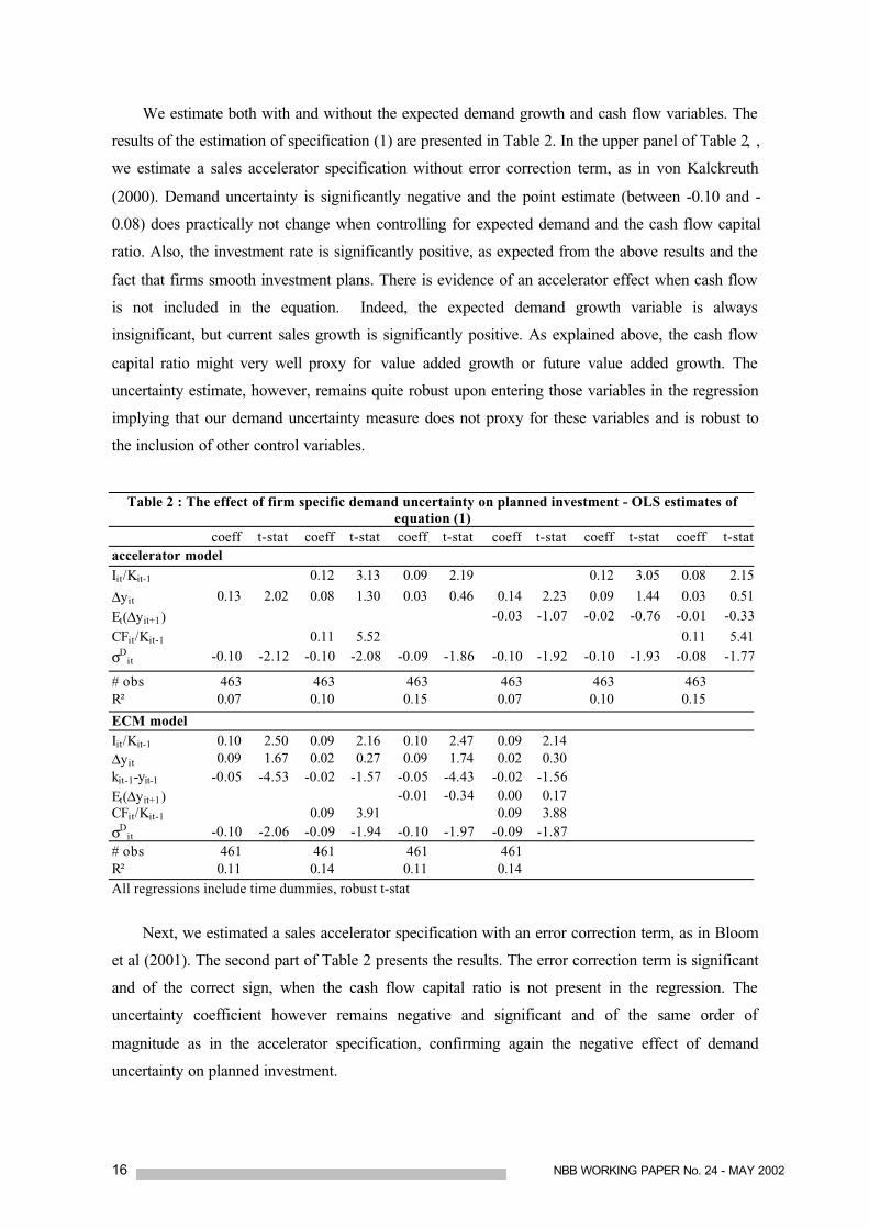
We estimate both with and without the expected demand growth and cash flow variables. The
results of the estimation of specification (1) are presented in Table 2. In the upper panel of Table 2, ,
we estimate a sales accelerator specification without error correction term, as in von Kalckreuth
(2000). Demand uncertainty is significantly negative and the point estimate (between -0.10 and -
0.08) does practically not change when controlling for expected demand and the cash flow capital
ratio. Also, the investment rate is significantly positive, as expected from the above results and the
fact that firms smooth investment plans. There is evidence of an accelerator effect when cash flow
is not included in the equation. Indeed, the expected demand growth variable is always
insignificant, but current sales growth is significantly positive. As explained above, the cash flow
capital ratio might very well proxy for value added growth or future value added growth. The
uncertainty estimate, however, remains quite robust upon entering those variables in the regression
implying that our demand uncertainty measure does not proxy for these variables and is robust to
the inclusion of other control variables.
Table 2 : The effect of firm specific demand uncertainty on planned investment - OLS estimates ofequation (1)
coeff t-stat coeff t-stat coeff t-stat coeff t-stat coeff t-stat coeff t-stataccelerator modelIit/Kit-1 0.12 3.13 0.09 2.19 0.12 3.05 0.08 2.15
∆yit 0.13 2.02 0.08 1.30 0.03 0.46 0.14 2.23 0.09 1.44 0.03 0.51
Et(∆yit+1) -0.03 -1.07 -0.02 -0.76 -0.01 -0.33
CFit/Kit-1 0.11 5.52 0.11 5.41
σDit -0.10 -2.12 -0.10 -2.08 -0.09 -1.86 -0.10 -1.92 -0.10 -1.93 -0.08 -1.77
# obs 463 463 463 463 463 463R² 0.07 0.10 0.15 0.07 0.10 0.15
ECM modelIit/Kit-1 0.10 2.50 0.09 2.16 0.10 2.47 0.09 2.14∆yit 0.09 1.67 0.02 0.27 0.09 1.74 0.02 0.30kit-1-yit-1 -0.05 -4.53 -0.02 -1.57 -0.05 -4.43 -0.02 -1.56Et(∆yit+1) -0.01 -0.34 0.00 0.17CFit/Kit-1 0.09 3.91 0.09 3.88σD
it -0.10 -2.06 -0.09 -1.94 -0.10 -1.97 -0.09 -1.87# obs 461 461 461 461R² 0.11 0.14 0.11 0.14All regressions include time dummies, robust t-stat
Next, we estimated a sales accelerator specification with an error correction term, as in Bloom
et al (2001). The second part of Table 2 presents the results. The error correction term is significant
and of the correct sign, when the cash flow capital ratio is not present in the regression. The
uncertainty coefficient however remains negative and significant and of the same order of
magnitude as in the accelerator specification, confirming again the negative effect of demand
uncertainty on planned investment.

NBB WORKING PAPER No. 24 - MAY 2002 17
Finally, we estimated a sales accelerator specification with valued added over capital and no
error correction term, as in Guiso and Parigi (1999). Table 3 presents our estimates of equation (2).
Uncertainty is significantly negative and the point estimate is practically identical to the one found
above. It does practically not change when controlling for the value added capital ratio and the cash
flow capital ratio. Again, cash flow seems to dominate the planning decision rendering value added
insignificant. Because cash flow might proxy for value added or future value added, this should not
be interpreted as if value added is irrelevant for the investment decision, as it results from
multicollinearity between value added and cash flow. The uncertainty estimate remains significantly
negative, indicating that our results provide robust evidence of a quite independent effect from the
other factors determining investment. The results of estimating the same regressions including the
expected demand variable indicate, as before, that the expected demand variable is always
insignificant. The coefficient of firm-specific demand uncertainty again implies a small response of
investment to uncertainty. A one standard deviation increase in firm-specific demand uncertainty
(i.e. 0.19) reduces the rate of investment plans rates by 7.5%.
Table 3: The effect of firm specific demand uncertainty on planned investment - OLS estimates ofequation (2)
coeff t-stat coeff t-stat coeff t-stat coeff t-stat coeff t-stat coeff t-statIit/Kit-1 0.08 2.28 0.11 3.00 0.13 3.44 0.08 2.26 0.11 2.98 0.13 3.4Yit/Kit 0.001 0.41 0.01 4.89 0,00 0.38 0.01 4.79
Et(∆yit+1) -0.01 -0.29 -0.006 -0.24 -0.01 -0.49CFit/Kit-1 0.11 4.71 0.11 4.71
σDit -0.09 -1.94 -0.10 -2.05 -0.10 -2.15 −0,09 -1.87 -0.10 -1.98 -0.10 -2.04
# obs 473 473 473 473 473 473R² 0.15 0.11 0.09 0.15 0.11 0.09
All regressions include time dummies, robust t-stat
In sum, from the estimations with sector-specific uncertainty and those with firm-specific
uncertainty, there is robust evidence that demand uncertainty reduces investment plans, although the
size of this effect may be of limited magnitude. A one standard deviation increase in demand
uncertainty reduces the rate of investment by 3% to 7.5% of its mean. For comparison, von
Kalckreuth (2002) find an effect of the same order of magnitude (6.5%). Further, firms smooth
investment and there is evidence of an accelerator effect, although these results are sometimes
blurred by the inclusion of cash-flow.
5.2. Euler equation
The next two tables present the Euler equation estimates. These were obtained by using the
OLS-estimator on orthogonal deviations (an alternative transformation to the within transformation

18 NBB WORKING PAPER No. 24 - MAY 2002
suggested by Arellano and Bover, 1995). In order for the OLS estimates to be consistent, this
transformation only requires that the regressors be non-contemporaneously correlated with the error
term. The more traditional transformations to eliminate the fixed effects, i.e. within and first
differences, need the more severe requirement that the regressors are strictly exogenous. Of course,
the current investment rate to some extent determines current sales and the wage sum. One might,
however, expect that endogeneity is only weak, since current investment is only a minor fraction of
the capital stock, which enters the production function. In addition, we can reasonably expect that
the investment rate determines sales growth, as in the accelerator specification, more than the levels
of sales. So, in fact there is a trade-off between using simple OLS and accepting a weak
endogeneity bias, or using an instrumental variable estimator and accepting the danger of weak
instruments. We prefer the former option. Moreover, since we use observed investment plans, we
can avoid a forecast error bias, which is introduced by assuming rational expectations and replacing
unobserved expectations by realised values. Especially, the presence of this forecast error explains
why instrumental variable techniques are common practice in the literature. This practice is less
inevitable with our data set.
For the Autumn survey, the results in table 4 indicate that the adjustment cost parameter is
significant and that output price uncertainty depresses current investment. Demand uncertainty,
however, is not significant. Although a similar result was obtained by Peeters (2001) for a sample of
large Belgian manufacturing firms, it does not confirm our previous results. We obtain reasonable
estimates (1.22) of the price elasticity of demand, which point to monopolistic forces being present.
This coefficient is, however, not significant.
For the Spring survey, the adjustment cost parameter is again significant. We obtain a similar
estimate for the price elasticity of demand (1.33) as in the Autumn survey, but now the coefficient is
significant at the 15% level. Both demand and output price uncertainty depress current investment,
although the latter effect is not significant, when both uncertainty terms are simultaneously entered
in the equation. The demand uncertainty effect clearly dominates. This corresponds to the results of
the other specifications in this paper. To summarise, demand uncertainty has a negative impact on
investment in t (or on the level of investment in any period, when solving the model forward). The
impact of demand uncertainty on the gap between future and current investment (the LHS variable),
however, is positive. This implies that uncertainty depresses current investment more than future
investment. This confirms the timing feature of the real option theory: uncertainty delays
investment decisions.

NBB WORKING PAPER No. 24 - MAY 2002 19
Table 4 : Euler equation estimates
Autumn Surveycoeff t-stat coeff t-stat coeff t-stat coeff t-stat
witLit/pIitKit 0.07 4.91 0.04 2.70 0.04 2.68 0.04 2.70
PitYit/PIitKit -0.02 -0.63 -0.01 -0.62 -0.01 -0.60 -0.01 -0.61
Et(PIit+1/PI
it) -0.31 -1.85 -0.31 -1.80 -0.31 -1.83 -0.31 -1.80
σDit . -0.02 -0.12 0.10 0.81 .
σPit . 0.37 2.02 . 0.36 2.18
α 24.45 24.51 24.75 24.56ε 1.23 1.22 1.22 1.22# obs - #firms 5885 1349 5885 1349 5885 1349 5885 1349R²adj 0.01 0.01 0.01 0.01
Spring Surveycoeff t-stat coeff t-stat coeff t-stat coeff t-stat
witLit/pIitKit 0.07 4.91 0.07 4.88 0.07 4.87 0.07 4.92
PitYit/PIitKit -0.02 -1.51 -0.02 -1.47 -0.02 -1.46 -0.02 -1.50
Et(PIit+1/PI
it) 0.04 0.22 0.05 0.31 0.05 0.29 0.05 0.29
σDit . 0.33 2.29 0.42 3.24 .
σPit . 0.25 1.38 . 0.44 2.68
α 13.77 13.86 13.90 13.75ε 1.33 1.32 1.32 1.32# obs - #firms 7459 1549 7459 1549 7459 1549 7459 1549R²adj 0.01 0.01 0.01 0.01
All regressions include time dummies
Next, we investigate the effect of irreversibility. The Spring survey contains information on
the type of investment: buildings or machines. One can reasonably consider buildings to be more
multi purpose, hence more reversible, and machines to be more firm-specific made, hence more
irreversible. According to the real option theory, the effect of uncertainty on the former type of
investment should be weaker than on the latter type. To analyse this, we include in our equation
interaction terms between uncertainty and a measure for the relative importance of a particular type
of investment, i.e. its share in total investment. Our results, shown in table 5, confirm the priors.
The more a firm invests in buildings, the smaller is the impact of uncertainty. The reverse applies
for machine investments. For leased equipment, which in the literature is often regarded as being
less irreversible (Cassimon et al, 2002, Guiso and Parigi, 1999) and, thus, being less sensible to
uncertainty, we find rather puzzling the opposite effect. This may perhaps be due to the fact that
only a limited number of firms use this method of financing, so that this variables may not provide a
relevant proxy of the degree of irreversibility.
We additionally performed an estimate including the leverage ratio. These results, which are
available on request, confirm the results presented in tables 4 and 5. Guiso and Parigi (1999) argue
that omitting a proxy for financial constraints effects, could bias the estimates for the uncertainty
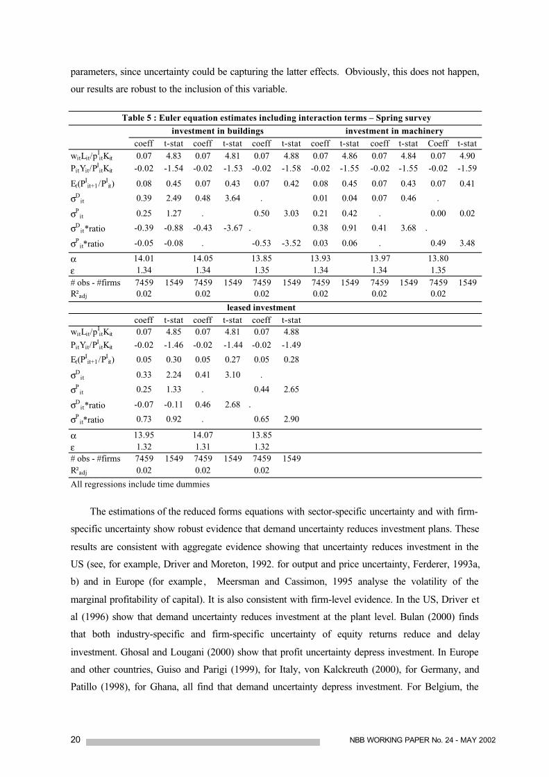
20 NBB WORKING PAPER No. 24 - MAY 2002
parameters, since uncertainty could be capturing the latter effects. Obviously, this does not happen,
our results are robust to the inclusion of this variable.
Table 5 : Euler equation estimates including interaction terms – Spring survey
investment in buildings investment in machinerycoeff t-stat coeff t-stat coeff t-stat coeff t-stat coeff t-stat Coeff t-stat
witLit/pIitKit 0.07 4.83 0.07 4.81 0.07 4.88 0.07 4.86 0.07 4.84 0.07 4.90
PitYit/PIitKit -0.02 -1.54 -0.02 -1.53 -0.02 -1.58 -0.02 -1.55 -0.02 -1.55 -0.02 -1.59
Et(PIit+1/PI
it) 0.08 0.45 0.07 0.43 0.07 0.42 0.08 0.45 0.07 0.43 0.07 0.41
σDit 0.39 2.49 0.48 3.64 . 0.01 0.04 0.07 0.46 .
σPit 0.25 1.27 . 0.50 3.03 0.21 0.42 . 0.00 0.02
σDit*ratio -0.39 -0.88 -0.43 -3.67 . 0.38 0.91 0.41 3.68 .
σPit*ratio -0.05 -0.08 . -0.53 -3.52 0.03 0.06 . 0.49 3.48
α 14.01 14.05 13.85 13.93 13.97 13.80ε 1.34 1.34 1.35 1.34 1.34 1.35# obs - #firms 7459 1549 7459 1549 7459 1549 7459 1549 7459 1549 7459 1549R²adj 0.02 0.02 0.02 0.02 0.02 0.02
leased investmentcoeff t-stat coeff t-stat coeff t-stat
witLit/pIitKit 0.07 4.85 0.07 4.81 0.07 4.88
PitYit/PIitKit -0.02 -1.46 -0.02 -1.44 -0.02 -1.49
Et(PIit+1/PI
it) 0.05 0.30 0.05 0.27 0.05 0.28
σDit 0.33 2.24 0.41 3.10 .
σPit 0.25 1.33 . 0.44 2.65
σDit*ratio -0.07 -0.11 0.46 2.68 .
σPit*ratio 0.73 0.92 . 0.65 2.90
α 13.95 14.07 13.85ε 1.32 1.31 1.32# obs - #firms 7459 1549 7459 1549 7459 1549R²adj 0.02 0.02 0.02
All regressions include time dummies
The estimations of the reduced forms equations with sector-specific uncertainty and with firm-
specific uncertainty show robust evidence that demand uncertainty reduces investment plans. These
results are consistent with aggregate evidence showing that uncertainty reduces investment in the
US (see, for example, Driver and Moreton, 1992. for output and price uncertainty, Ferderer, 1993a,
b) and in Europe (for example , Meersman and Cassimon, 1995 analyse the volatility of the
marginal profitability of capital). It is also consistent with firm-level evidence. In the US, Driver et
al (1996) show that demand uncertainty reduces investment at the plant level. Bulan (2000) finds
that both industry-specific and firm-specific uncertainty of equity returns reduce and delay
investment. Ghosal and Lougani (2000) show that profit uncertainty depress investment. In Europe
and other countries, Guiso and Parigi (1999), for Italy, von Kalckreuth (2000), for Germany, and
Patillo (1998), for Ghana, all find that demand uncertainty depress investment. For Belgium, the

NBB WORKING PAPER No. 24 - MAY 2002 21
results of Peeters (2001) suggest that price uncertainty reduces investment of large firms, but not
demand uncertainty. Gérard and Verschueren (2002) also find little empirical support for an effect
of investment price uncertainty on investment in a sample of Belgian firms. This may be due to the
type of uncertainty (investment prices) they consider, and to the way uncertainty was measured;
both Peeters and Gérard and Verschueren use a time-invariant volatility measure interacted with a
time-varying assets to equity ratio. On the contrary, Cassimon et al (2002) show that uncertainty of
profitability diminishes the probability and amount of investment. Finally, consistently with
Cassimon et al (2002), Guiso and Parigi (1999) and Patillo (1998), we also find that the effect of
uncertainty on investment is larger for firms with more irreversible investment.

22 NBB WORKING PAPER No. 24 - MAY 2002
6. CONCLUSIONS
In this paper we investigate how demand and output price uncertainty affect investment plans
of Belgian manufacturing firms. We obtain time-varying uncertainty measures at the firm and
industry level from the Belgian monthly business cycle survey and investment plans from the half-
yearly investment survey. Using investment plans instead of realised investment data, e.g. annual
accounts data, is from an informative point of view superior, since it is more likely to reveal the
features of the decision formation process and therefore is most closely related to economic theory.
Business investment is normally planned well in advance, because it involves time and costs to
implement, and theory describes the behaviour of firms at the moment of their decision, which can
be assumed to be fully captured in survey data. In order to find robust predictions we estimate three
different specifications, each of which can be considered as a benchmark in the literature: two
reduced form equations and a structural Euler equation.
Our results show that uncertainty depresses investment. These results hold for industry- as
well as for firm-specific demand uncertainty. Our time-varying uncertainty measures at the firm
and industry level enter significantly in three different investment specifications. The reduced form
estimates for both industry- and firm- specific uncertainty point to the same conclusion. We find
that industry- and firm-specific demand uncertainty negatively effects investment plans, where
industry- and firm-specific price uncertainty does not effect investment plans. The Euler equation
results however show a slightly different picture. Where sector price uncertainty is both significant
for the Spring and Autumn survey, we find demand uncertainty only to be significant in the Spring
survey. Moreover, the estimation of an Euler equation provides additional insight on the
investment-uncertainty relationship. Our results indicate that increased uncertainty induces firms to
postpone investment today in favour of investment tomorrow, and that this effect is stronger for
more irreversible capital. Hence, our results seem to confirm to predictions of the real option theory.
Our results show that unresolved specification issues in the uncertainty-investment literature
remain important. Where papers in this literature usually test for robustness within specifications
(by removing or entering extra variables to the regression or using different estimators), we test the
robustness of the effect of uncertainty across different specifications (Euler equation and reduced
form equation) and across data sets (Spring and Autumn survey, firm and sector uncertainty).
For policy purpose, the relevant question is whether aggregate uncertainty reduces realised
investment, and if so what is the best way to reduce the uncertainty of the economic environment.
By investigating the effect of uncertainty on planned investment, we really focus on the effect of an

NBB WORKING PAPER No. 24 - MAY 2002 23
uncertain environment on the decision of the firm about its investment projects. The realisation of
these projects may be subject to some discrepancies when new information arrives, but the project
is defined the period before. Concerning the type of uncertainty our results clearly show that
uncertainty reduces investment plans, but our analysis did not fully disentangle between firm-
specific or sector-specific and aggregate uncertainty, except to the extent that time dummies control
for common aggregate fluctuations in any variables. At least our results with sector-specific
uncertainty indicate that aggregate uncertainty matters for investment.

24 NBB WORKING PAPER No. 24 - MAY 2002
References
Abel, A. B. (1983), "Optimal investment under uncertainty", American Economic Review, 73, 228-233.
Abel, A. B. and J. C. Eberly (1994), "A unified model of investment under uncertainty", AmericanEconomic Review, 84, 1369-1384.
Abel, A. B. and J. C. Eberly (1999), "The effects of irreversibility and uncertainty on capitalaccumulation", Journal of Monetary Economics, 44, 339-377.
Abel, A.B., A.K. Dixit, J.C. Eberly and R.S. Pindyck (1996), "Options, the value of capital andinvestment", Quarterly Journal of Economics, 109, 753-777.
Arellano, M. and O. Bover (1995) "Another look at the instrumental variable estimation of error-components models", Journal of Econometrics, 68, 29-51
Arellano, M. and S. Bond (1991) "Some tests of specification for panel data: Monte Carlo evidenceand an application to employment equations", Review of Economic Studies, 58, 277-297
Barran, F. and M. Peeters (1998) "Internal finance and corporate investment. Belgian evidence withpanel data", Economic Modelling, 15, 67-89
Batchelor, R. A. (1986), "Quantitative v. qualitative measures of inflation expectations ", OxfordBulletin of Economics and Statistics, 48(2), 99-120.
Bertola, G. (1988), Adjustment costs and dynamic factor demands: investment and unemploymentunder uncertainty, Ph.D. Thesis, MIT.
Bloom, N., S. Bond and J. Van Reenen (2001), "The dynamics of investment under uncertainty",The Institute for Fiscal Studies, Working Paper n°5.
Bond, S., J. Elston, J. Mairesse and B. Mulkay (1997), "Financial factors and investment inBelgium, France, Germany and the UK: a comparison using company panel data", NBERWorking paper n° 5900.
Bulan, L. T. (2000), "Real options, irreversible investment and firm uncertainty: new evidence fromUS firms", mimeo.
Butzen, P., C. Fuss and P. Vermeulen (2001), "The interest rate and credit channels in Belgium: aninvestigation with micro-level firm data", National Bank of Belgium Working Paper ResearchSeries n°18.
Caballero, R. (1991), "On the sign of the investment-uncertainty relationship", American EconomicReview, 81, 279-288.
Carlson, J. A. and M. Parkin (1975), "Inflation expectations", Econometrica, 42, 123-138.

NBB WORKING PAPER No. 24 - MAY 2002 25
Carruth, A., A. Dickerson and A. Henley (2000), "What do we know about investment underuncertainty?", Journal of Economic Surveys, 14(2), 119-153.
Caselli, P., P. Pagano and F. Schivardi (2000), "Investment and growth in Europe and in the UnitedStates in the nineties", Banca d'Italia, Termi id discussione, n° 372.
Cassimon, D., P.-J. Engelen, H. Meersman, and M. Van Wouwe (2002), "The impact of uncertaintyon firms' investment decisions in Belgium: a micro-economic panel data approach", NationalBank of Belgium Working Paper, Research Series n°23
Chatelain, J.-B. and J.-C. Teurlai (2000) Comparing several specifications of financial constraintsand adjustment costs in investment Euler equations, Banque de France, mimeo
Dixit, A.K. and R.S. Pindyck (1994), Investment under uncertainty, Princeton University Press,Princeton, New Jersey.
Doms, M. and T. Dunne (1998), "Capital adjustment patterns in manufacturing plants", Review ofEconomic Dynamics, 1, 409-429.
Driver, C. and D. Moreton (1992), Investment expectations and uncertainty, Backwell publishers,Oxford, United Kingdom.
Driver, C., P. Yip and N. Dakhil (1996), "Large company capital formation and effects of marketshare turbulence: micro-data evidence from the PIMS database", Applied Economics, 28,641-651.
Eberly, J.C. (1997), "International evidence on investment and fundamentals", European EconomicReview, 41. 1055-1078.
Ferderer, J.P. (1993a), "The impact of uncertainty on aggregate investment spending. An empiricalanalysis", Journal of Money, Credit and Banking, 25(1), 30-48.
Ferderer, J.P. (1993b), "Does uncertainty affect investment spending?", Journal of Post-KeynesianEconomics, 16(1), 19-35.
Gérard, M. and F. Verschueren (2002), "Finance, uncertainty and investment: assessing the gainsand losses of a generalised non linear structural approach using Belgian panel data", NationalBank of Belgium Working Paper, Research Series n°26.
Ghosal, V. and P. Lougani (2000), "The differential impact of uncertainty on investment in smalland large businesses", Review of Economics and Statistics, 82(2), 338-349.
Guiso, L. and G. Parigi (1999), "Investment and demand uncertainty", Quarterly Journal ofEconomics, 185-227.

26 NBB WORKING PAPER No. 24 - MAY 2002
Hartman, R. (1972), "The effects of price and cost uncertainty on investment", Journal of EconomicTheory, 5, 258-266.
Houbedine, M. (2001), "Investment forecast and capacity utilisation: a panel data analysis", in Useof Survey Data for Industrial, research and Economic Policy.
Kaplan, S.N. and L. Zingales (1997) "Do investment cash flow sensitivities provide useful measuresof financing constraints?", Quarterly Journal of Economics, 112(1), 169-215.
Mc Donald, R. and D. Siegel (1986), "The value of waiting to invest", Quarterly Journal ofEconomics, 101, 707-728.
Meersman, H. and D. Cassimon (1997), "Investment in the EC-countries : does reducinguncertainty matter", SESO Report, n° 95/320.
Patillo, C. (1998), "Investment, uncertainty and irreversibility in Ghana", IMF Staff Papers, 45(3),522-553.
Peeters, M. (2001), "Does demand and price uncertainty affect Belgian and Spanish corporateinvestment?", Recherches Economiques de Louvain, 67 (3), 235-255.
Pindyck, R.S. (1993), "A note on competitive investment under uncertainty", The AmericanEconomic Review, 83, 273-277.
Pindyck, R.S. and A. Solimano (1993), "Economic stability and aggregate investment", PolicyResearch Working paper 114,. World Bank.
Price, S. (1995), "Aggregate uncertainty, capacity utilisation and manufacturing investment",Applied Economics, 27, 147-154.
Theil, H. (1952), "On the time shape of economic microvariables and the Munich business test",Review of the International Statistical Institute , 20, 105-120.
Vermeulen, P. (1998), Detecting the influence of financing constraints on fixed investment, mimeo.
von Kalckreuth, U. (2000), "Exploring the role of uncertainty for corporate investment decisions inGermany", Deutsche Bundesbank Discussion Paper, n° 5/00.

NBB WORKING PAPER No. 24 - MAY 2002 27
A. Data appendix
A.1. Data definitions
The real capital stock at time t is constructed by adjusting the book value of the capital stock at
time t by its average age. The book value of the capital stock at time t is defined as the sum of the
acquisition value of total tangible assets (code 8159) and revaluation gains (code 8209) minus
accumulated depreciation and amounts written down (code 8269), all at the end of the preceding
period. As in Chatelain and Teurlai (2000), the average age of the capital stock (A) is computed
from the share of the capital stock that has already been depreciated with the following formula:
A=15*(depr/book)-4 if 15*(depr/book)>8
A=15*(depr/book)*(1/2) if 15*(depr/book)<=8.
Where depr is accumulated depreciation (code 8269). The variable book is measured by the
acquisition value of total tangible assets (code 8159). To obtain the real capital stock at time t, the
book value at time t (code 8159 + code 8209 - code 8269) is divided by the investment price index
of t-A.
This method has two major advantages over the perpetual inventory method. First, it treats the
construction of the real capital stock equally in the beginning of the sample and at the end of the
sample. Second, where gaps in the data in terms of missing investment rates lead to breakage of the
perpetual inventory method, they do not lead to breaks for this method.
A.2. Data cleaning
The disconformity index lies between 0 and 1 by construction, and therefore cannot contain
outliers. So, we remove outliers of the other variables only.
For the estimates of the ECM equation with sector-specific uncertainty, investment rates are
trimmed by dropping the first and last decile 17. This yields investment rates that are not too much
above 100%. Sales growth and the cash-flow capital ratio are trimmed by dropping the first 5% and
17 Preliminary results (not reported here for the sake of brevity) show that less severe trimming leads to
identical qualitative conclusions, but the quality of the estimates (in particular the value of the Sargan test)dramatically deteriorates. This may be due to remaining outliers. We therefore use a sample trimmed bythe first and last decile.

28 NBB WORKING PAPER No. 24 - MAY 2002
last 5%. All trimmings are done year by year and for small and large firms separately. Table A.1 in
appendix shows some descriptive statistics after cleaning. Initially, the investment survey matched
with annual accounts and sector-specific prices yield a sample of 10162 observations and 1992
firms. The maximum values of investment rates clearly indicates the presence of outliers. After
trimming and first differencing, our sample has 3090 observations and 930 firms with at least one
year of observation. Finally, in order to perform the first difference GMM estimations, we have to
restrict this sample by keeping only those firms, which have at least 5 surveys and 6 annual
accounts. We end up with a sample of 1303 observations and 256 firms. All variables lie in
reasonable ranges. In the final sample, more than 85% of the firms are large. Clearly our sample
suffers from a severe selection bias towards large firms, as the percentage of large firms in the
whole economy is around 7.5%. Further our sample does not cover all sectors of the economy, since
the investment survey focus on manufacturing industries.
Table A.1. Descriptive statistics of the ECM sector-specific uncertainty model
# obs mean std, dev min maxInitial sample (1987-2000) - 1992 firmsIP
it+1 /Kit 10162 2.65 107.09 0.00 9713.49
Iit/Kit-1 10162 0.84 15.56 0.00 1075.25
After matching trimmed investment plans with trimmed variables (1987-1999) - 930 firmsIP
it+1 /Kit 3090 0.26 0.15 0.04 0.97
Iit/Kit-1 3090 0.26 0.17 0.03 1.32
∆yit 3090 0.01 0.14 -0.54 0.44
CFit/Kit 3090 0.48 0.38 -0.30 3.43
yit 3090 15.72 1.65 10.71 20.92kit-1 3090 14.90 1.86 9.51 20.82
σDst 3090 0.34 0.06 0.09 0.54
σPst 3090 0.26 0.05 0.04 0.46
Et(∆yit+1) 3090 -0.07 0.14 -0.47 0.19
Sample of firms with at least 5 surveys and 6 annual accounts - 256 firms
IPit+1 /Kit 1303 0.26 0.14 0.04 0.72
Iit/Kit-1 1303 0.26 0.15 0.03 0.87
∆yit 1303 0.01 0.13 -0.39 0.40
CFit/Kit 1303 0.47 0.34 -0.30 2.59
yit 1303 16.14 1.59 11.98 20.59kit-1 1303 15.33 1.74 10.40 20.78
σDst 1303 0.35 0.05 0.09 0.54
σPst 1303 0.26 0.05 0.05 0.37
Et(∆yit+1) 1303 -0.09 0.14 -0.47 0.16
For the estimates with firm-specific uncertainty, we restrict our sample to firms for which we
have a firm-specific uncertainty measure (that is for firms, which answered the NBB business,

NBB WORKING PAPER No. 24 - MAY 2002 29
survey every month). We remove the first and last percentiles of the variables in the regression,
except for the investment and planned investment ratio for which we use the first and 95th
percentile. Our final data set contains 473 firm-year observations 18. Table A.2 reports descriptive
statistics for this sample. The data set is unbalanced with most firms having only a few
observations.
Table A.2. Descriptive statistics of the firm-specific uncertainty model
# obs mean std, dev min MaxIP
it+1 /Kit 473 0.25 0.20 0.01 1.03
σDit 473 0.22 0.19 0.00 0.91
Iit/Kit-1 473 0.30 0.27 0.01 1.44
Yit/Kit-1 473 2.60 2.60 0.23 23.73
∆yit 463 -0.003 0.16 -0.77 0.71
Et(∆yit+1) 473 -0.11 0.39 -1.00 0.92CFit/Kit-1 473 0.50 0.45 -1.13 2.93
18 However most regressions contain fewer observations due to the fact that not all control variables are
available for all firms. For the Spring survey and actual investment data we have a few less observations,since not all firms answered both Spring and Autumn survey.
30 NBB WORKING PAPER No. 24 - MAY 2002
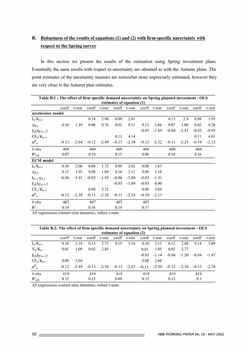
B. Robustness of the results of equations (1) and (2) with firm-specific uncertainty with
respect to the Spring survey
In this section we present the results of the estimation using Spring investment plans.
Essentially the same results with respect to uncertainty are obtained as with the Autumn plans. The
point estimates of the uncertainty measure are somewhat more imprecisely estimated, however they
are very close to the Autumn plan estimates.
Table B.1 : The effect of firm specific demand uncertainty on Spring planned investment - OLSestimates of equation (1)
coeff t-stat coeff t-stat coeff t-stat coeff t-stat coeff t-stat coeff t-stataccelerator modelIit/Kit-1 0.14 2.90 0.09 2.01 0.13 2.8 0.09 1.95
∆yit 0.10 1.39 0.06 0.76 0.01 0.11 0.12 1.66 0.07 1.00 0.02 0.28
Et(∆yit+1) -0.05 -1.69 -0.04 -1.41 -0.03 -0.95
CFit/Kit-1 0.11 4.14 0.11 4.01
σDit -0.13 -2.64 -0.12 -2.49 -0.11 -2.30 -0.12 -2.32 -0.11 -2.23 -0.10 -2.12
# obs 409 409 409 409 409 409R²adj 0.07 0.10 0.15 0.08 0.10 0.16
ECM modelIit/Kit-1 0.10 2.08 0.08 1.72 0.09 2.02 0.08 1.67
∆yit 0.15 1.95 0.08 1.04 0.16 2.11 0.09 1.18
kit-1-yit-1 -0.06 -3.91 -0.03 -1.95 -0.06 -3.80 -0.03 -1.91
Et(∆yit+1) -0.03 -1.09 -0.03 0.90
CFit/Kit-1 0.09 3.12 0.09 3.04
σDit -0.12 -2.38 -0.11 -2.28 -0.11 -2.18 -0.10 -2.11
# obs 407 407 407 407R² 0.14 0.16 0.14 0.17All regressions contain time dummies, robust t-stats
Table B.2: The effect of firm specific demand uncertainty on Spring planned investment - OLSestimates of equation (2)
coeff t-stat coeff t-stat coeff t-stat coeff t-stat coeff t-stat coeff t-statIit/Kit-1 0.10 2.19 0.13 2.73 0.15 3.16 0.10 2.15 0.12 2.68 0.14 3.09Yit/Kit 0.01 1.09 0.02 2.85 0,01 1.05 0.02 2.77
Et(∆yit+1) -0.03 -1.14 -0.04 -1.20 -0.04 -1.47CFit/Kit-1 0.08 2.69 0.08 2.66
σDit -0.12 -2.49 -0.13 -2.56 -0.13 -2.63 −0,11 -2.30 -0.12 -2.36 -0.12 -2.38
# obs 419 419 419 419 419 419R²adj 0.15 0.13 0.09 0.15 0.13 0.1
All regressions contain time dummies, robust t-stats

NBB WORKING PAPER No. 24 - MAY 2002 31
C. The derivation of the Euler equation
1. Dividends at any given time t+s (s going from 0 to infinite) are given by
),(**),( ststI
ststI
ststststI
ststststst IKpIpNwKpNKFpD +++++++++++++ Φ−−−−= σθ
with the last term being the adjustment cost function. We allow for imperfect competition
(downward sloping demand curve) by letting the price being a function of output. Uncertainty
enters as a cost for the firm if 0>θ . Let the adjustment cost function be the traditional quadratic
adjustment cost ),( tt IKΦ = tt
t KK
I 2][2
φα − .
2. the firm is at time t and has to maximise its future and current (at time t) dividends i.e. the
following objective
sts
jt
s
jt DE +
∞
=+
=∑ Π
0 0
)( β
where the βs are the discount factors assumed as being given an certain. (One should also assume
βt=1. since contemporaneous dividend should be discounted at 1)
3. capital accumulation is given by
ttt IKK +−= −1)1( δ
A solution of the maximisation problem can be found by writing down the problem as a Lagrangian
Problem:
L=
])1([)(
)],(),()([)(
10 0
0 0
tttsts
jt
s
jt
ststI
ststI
stsitI
sitstststststs
jt
s
jt
IKKE
IKpIpKpNwNKFFpE
−−−−
Φ−+−−
−+
∞
=+
=
++++++++++++
∞
=+
=
∑ Π
∑ Π
δλβ
θσβ
With st +λ a Lagrange multiplier

32 NBB WORKING PAPER No. 24 - MAY 2002
The first order conditions of this problem are the following:
1) FOC w.r.t Kt : 0E)1()]I,K(pp*)N,K(Fp)1
1[( 1t1tttttKItst
ItttKt =λβδ−+λ−Φ−σθ−
ε− ++
2) FOC w.r.t. Nt : 0w)N,K(Fp)1
1( tttKt =−ε
−
3) FOC w.r.t. It : 0)],([ =+Φ−− tttIIt
It IKpp λ
4) FOC w.r.t. It+1 :
0)],([ 1111111 =+Φ−− +++++++ tttttIIt
Ittt EIKppE λββ
The investment equation can then be found by replacing in 1) the tλ by using 3) and tttE λβ 1+ by
using 4). We get:
]p
pE)1(
p
p[
)1(
1]
p
p)1(
2[
p
p
)1(
1
)K
I(
p
p
)1(
1)
K
I(
p
p
)1(2
1
p
p*
)1(
1)N,K(F
p
p
)1(
)1
1(1)
K
I(E
I1t
I1t
t1tI1t
It
1tIt
I1t
1t2
I1t
It
1t
t
tI
1t
It
1t
2
t
tI
1t
It
1tstI
1t
It
1tttKI
1t
t
1t1t
1tt
+
++
++
++
++
+++++++++
+
βδ−−αβδ−
+αφβδ−+αφ−αφαβδ−
+
βδ−+
βδ−−+σ
αθ
βδ−+
αβδ−ε
−−=
or , after assuming constant returns to scale and applying Euler's theorem to proxy the MRPK
]p/)p(E)1)(1(12
[1
*)K
L
p
w(
1)
K
F
p
p(
)1
1()K/I(
2
1)K/I()Kp/Ip(E)1(
It
I1tit1iti
2
stit
itIit
it
it
itIt
it2itititit1it
It1it
I1tt1iti
++
++++
βδ−−αφ+αφ−+αφα
+
+σαθ+
α+
αε
−−=+−βδ−


