4

NASA TECHNICAL NOTE ,NASA JN _O-SlOS z e

4 c/)4 z

-LOAN COPY: RETURN TO A FINITE-DIFFERENCE ANALYSIS TECHNICAL LIBRARY

OF THE NOZZLE STARTING PROCESS KIRTLAND AFB, Me M.

I N A N EXPANSION TUNNEL ,,/;T ;

I '\>

K. Jumes Wedmuenster i' ,

I

Langley Research Center \ \\ .

Hdmpton, Va. 23665

N A T I O N A L AERONAUTICS A N D SPACE A D M I N I S T R A T I O N W A S H I N G T O N , D. C. DECEMBER 1975

https://ntrs.nasa.gov/search.jsp?R=19760006332 2018-05-21T17:50:21+00:00Z

1­. . .­-

1. Report No. 2. Government Accession No. 3. Recipient's Catalog No.

NASA TN D-8105 5. Report Date

December 1975 6. Performing Organization Code

8. Performing Organization Report No.

L- 10500 10.Work Unit No.

506-2 6-20-0 1 11. Contract or Grant No.

13. Type of Report and Period Covered

Technical Note 14. Sponsoring Agency Code

I ~

16. Abstract

A suitable finite-difference method for computing the quasi-one-dimensional unsteady flow in an expansion tunnel nozzle has been identified. The difference equations a r e pre­sented along with the appropriate stability limits. A parametr ic study of the s tar t ing process

17. Key-Words (Suggested by Authoris) ) 18. Distribution Statement

Finite difference Unclassified - Unlimited Unsteady flow Nozzle flow

Subject Category 34 - ­

19.Security Classif. (of this report) 20. Security Classif. b f this page) 21.NO. of Pages 22. Price'

Unclassified Unclassified 47 $3.75

For sale by the National Technical Information Service, Springfield, Virginia 22161

A FINITE-DIFFERENCE ANALYSIS O F THE

NOZZLE STARTING PROCESS IN

AN EXPANSION TUNNEL

K. James Weilmuenster Langley Research Center

SUMMARY

A finite-difference solution of the time-dependent, quasi-one-dimensional equations for a bigas mixture, including real gas effects, for both viscous and inviscid flow has been applied to the starting process in an expansion tunnel nozzle.

An analysis of the numerical technique has shown that using a Richtmyer differencing solution of the inviscid quasi-one-dimensional equations along with a smoothing function avoids numerical instabilities unrelated to classical stability c r i te r ia and that the stability restriction on step size for the quasi-one-dimensional equations is identical to that for the one-dimensional equations.

The solutions obtained for the starting process in a conical nozzle 1.732 m in length indicate that expansion tunnel operation without a ternery diaphragm is restricted to those conditions for which the test flow is not disrupted by an upstream-facing shock and that the use of a ternery diaphragm in the system, combined with a sufficiently low initial nozzle pressure, wil l allow the nozzle to be started in an acceptable manner.

INTRODUCTION

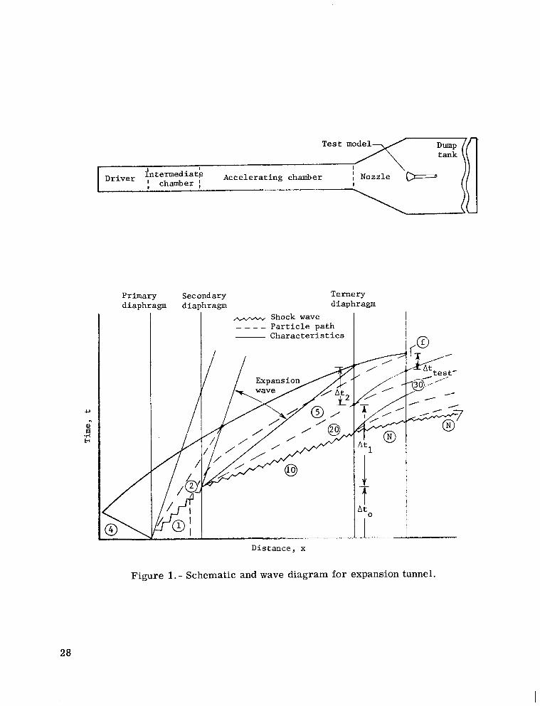
The development and analysis of the expansion tube, a device used to produce high-stagnation enthalpy flows, have been thoroughly discussed in several papers (refs. 1to 4). The expansion tunnel is a modification of the expansion tube which utilizes the basic expan­sion tube configuration with a ternery diaphragm and a conical nozzle added a t the down­stream end of the acceleration chamber as illustrated in figure 1.

Trimpi and Callis (ref. 5) have made a perfect gas analysis of the expansion tunnel. Their calculations determined, among other things, the test time lost as a result of the starting and stopping processes in the nozzle, as well as those conditions which must be satisfied i f there is to be a perfect nozzle start (e.g., that no upstream compression waves be produced by the passage of the primary shock through the nozzle (see ref. 6)).

Friesen and Moore (ref. 7) measured velocity profiles and pitot pressure in the exit plane of an expansion tunnel nozzle. They investigated the two possible modes of expan­sion tunnel operation. First, the facility can be operated without a ternery diaphragm, which results i n the gas and initial pressure in the nozzle and dump tank being the same as that found in the acceleration chamber. Second, the ternery diaphragm can be used, which allows the gas and initial pressure in the nozzle and dump tank to be varied. Using the shock in the acceleration chamber to burst the ternery diaphragm is a good approxima­tion of the assumption of an instantaneous diaphragm opening used in the theoretical anal­ysis of the expansion tunnel. However, experiments have shown that allowing the incident shock in the acceleration chamber to burst the ternery diaphragm may degrade the quality of the flow entering the nozzle. Therefore, Friesen and Moore employed an electromag­netically opened diaphragm whose construction and effect on the flow entering the nozzle are detailed in reference 8. Essentially, they found that it was necessary to use a ternery diaphragm and to evacuate the nozzle before reasonably uniform nozzle exit conditions could be found.

The results of reference 5 are limited to those initial conditions for which no upstream-facing shock is generated in the nozzle. In order to extend the analysis of expansion tunnel operation to conditions which generate shocks in the nozzle and to make parametric studies of the effect of these shock waves on the test flow quality, i t has been necessary to develop a shock-capturing, finite-difference method for solving the funda­mental equations of quasi-one-dimensional flow.

A finite-difference method for solving the time-dependent, quasi-one-dimensional equations for a real, bigas flow is investigated for both viscous and inviscid flow. The method deemed to be most appropriate has been used to analyze the starting process in an expansion tunnel. Specifically, the effect of initial nozzle pressure and the formation of internal shocks on the starting process and the available test time a r e investigated.

SYMBOLS

A nozzle cross-sectional area, m2

-A area ratio, A(X)/A(X = 0)

a sound speed, m/s

B,c,F~J3coefficient matrices K,L,Q

cP specific heat at constant pressure, m2/s2-K

2

CV specific heat at constant volume, m2/s2-K

D nozzle diameter, m

E

e

f,g,S

k

P

RS

T

t

A t

U

U

W

total energy, p

internal energy, m2/s2

vector-valued functions

p thermal conductivity, N/s-K

incident shock Mach number in re@on@

molecular weight of species s, g mole

Prandtl number

Reynolds number

pressure, N/m2

gas constant of species s , m2/s2-K

temperature, K

time, s

time increment, s

free-stream velocity, m/s

velocity, m/s

vector of dependent variables

3

I

i

W mass fraction

X distance, m

Ax spatial increment, M

Y ratio of specific heats

6 nozzle half -angle, deg

E e r r o r in solution as function of time and space

x mesh ratio, At/&

P viscosity, N-s/m2

V eigenvalue of amplification matrix

P density , kg/m3

Subscripts:

0 region (see fig. 1)

j part of a sequence

mix property of gas mixture

0 initial o r reference value

S particular species

Superscript :

,. dimensional quantity

Abbreviation:

sss secondary starting shock

4

I

STATEMENT OF PROBLEM

The manner in which the starting flow in an expansion tunnel nozzle develops, for a given set of test conditions, has a direct effect upon the operation of the facility. Specifi­cally, the experimental results of Fr iesen and Moore (ref. 7) indicated that an electromag­netically opened ternery diaphragm had to be included in the system before a uniform test flow could be established at the nozzle exit. The addition of this hardware increases the system maintenance time between tunnel runs as well as adding further complexity to the facility operation. Also, much of the facility turnaround time is spent evacuating the var­ious sections of the system of which the nozzle dump tank is by far the largest. Obviously, higher allowable initial nozzle pressures will require shorter pumping times. Since Friesen and Moore maintained the initial nozzle pressure at approximately t o r r (1to r r = 133.3 N/m2), the effect of initial nozzle pressure on the nozzle starting process is unlmown.

In this report , a numerical method is developed to determine what usable test flows can be generated, for the given nozzle geometry and initial entrance conditions, without the use of a ternery diaphragm, and what is the maximum allowable initial nozzle pressure when operating with a ternery diaphragm in the system and the penalty for exceeding this value.

The paper deals with the starting process in a conical nozzle having an entrance diameter of 0.076 m and a length of 1.609 m, whose entrance conditions correspond to those found in the acceleration chamber of an expansion tube (i.e., a low-Mach-number flow followed by a high-Mach-number flow). These dimensions conform to those of a nozzle presently installed in the Langley 6-inch expansion tube. In the operation of an expansion tunnel, three different gases come into play: the test gas, initially in the inter­mediate chamber, the acceleration gas, initially in the acceleration chamber, and the gas initially in the nozzle, all of which may be the same o r different. In this study, only two different gases wil l be used at any one time. Thus, it will be necessary to include the dynamics and thermodynamics of a bigas flow in the analysis.

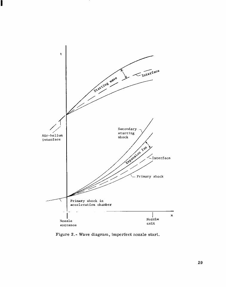
A wave diagram for the flow that might be expected for an imperfectly started noz­zle is indicated in figure 2. The gas initially in the acceleration chamber, which is pro­cessed by the primary shock, and the gas initially in the nozzle may o r may not be identical o r have identical pressures, depending on whether o r not there is a diaphragm separating the nozzle from the rest of the system. For the computations in this report, it is assumed that i f a ternery diaphragm does exist in the system, the diaphragm opens instantaneously upon contact with the incident shock. In the nozzle, the strength of the primary shock is decreased by the increasing area ratio while an interface separates the shocked acceleration-chamber gas from the shocked nozzle gas and an unsteady expansion fan .

5

This region of unsteady flow is terminated by an upstream-facing secondary starting shock. The secondary starting shock is followed by the steady expansion of the shocked acceleration gas. As the interface separating the shocked acceleration gas and the test gas t raverses the nozzle, it is accelerated and is preceded by a family of downstream-facing characteristics and followed by a family of upstream-facing characteristics. When the last of these has passed the nozzle exit, the nozzle is fully started. Test time in the nozzle is terminated by the arr ival of the trailing edge of the expansion tube expansion fan at the nozzle exit.

METHOD OF SOLUTION

Several investigations have been made of the starting process in a hypersonic noz­zle, most of which were performed in reflected shock tunnels. Perhaps the best known of these studies was published by Smith (ref. 9), who used the method of characteristics and a perfect gas to obtain solutions. More recently, Stalker and Mudford (ref. 10) made an experimental and simplified analytical analysis of the starting process in a nonreflected shock tunnel.

The analysis of hypersonic flows in nozzles by using finite-difference solutions was f i r s t investigated by Crocco (ref. 11). Crocco utilized the quasi-one-dimensional equa­tions in his work which concentrated on the stability of such a system rather than on the solution of any particular problem. Laval (ref. 12) used a two-step, second-order­accurate differencing scheme that employed an explicit artificial viscosity along with the quasi-one-dimensional equations to solve the reflected shock tunnel starting problem and obtained results which were i n good agreement with those of Smith (ref. 9). Laval also used a perfect gas. Benison and Rubin (ref. 13) used a variation of the Richtmyer method to solve the quasi-one-dimensional equations for a perfect gas including the effects of viscosity and heat conduction. They, however, limited their calculations to flows contain­ing only weak shocks.

Since the end result of this study is to provide time histories of nonlinear distur­bances as they t raverse a nozzle, the finite-difference scheme used should be second-order accurate in both time and space to insure good space-time resolution. A survey of available methods led to the choice of the Richtmyer differencing scheme as developed by Thommen (ref. 14) for use in this analysis. This method closely resembles the Benison-Rubin method yet requires fewer numerical computations. Also, there is some ambiguity associated with the specification of the upstream boundary conditions in the Laval method. In addition, the effects of imperfect gases and bicomponent flow, which would unduly com­plicate a characteristics solution, a r e included in the present analysis.

Briefly, the Richtmyer method is as follows. Given the partial differential equation of the form

the Richtmyer method takes on the form

At[ ( ;t y)- f ( t + y , x - k)]+ At[s(W),] t W(t + At,x) = W(t,x) - -f t + -,x + -

Ax 2 X

where

w t + - x * - 2)= i[W(t.,x) + W(t,x f Ax)1J T -At If(t,x) - f(t,x f Ax)1( y , 2 A x

This method is the result of a Taylor s e r i e s expansion of W about the point x and gains i t s second-order accuracy through the use of an intermediate step.

Details of the Richtmyer method a r e developed as follows. Expand W(t,x) about

2

2

and since Wt = -fx + Sx

+ O(At)2 (6)

7

I -

Then, i f W is expanded about the point W t + -,x ,

W(t + At,x) = W 3

3

Subtracting equation (9) from equation (8) and rearranging gives

W(t + At,x) = W(t,x) + AtWt 3

or with the substitution W t = -fx(W) + S(W),

W(t + At,x) = W(t,x) - Atf, 3

The spatial derivative f, is evaluated by using the values of W at

(t + At,x f -?. To maintain the formal second-order accuracy of equation (ll),second­

order-accurate central differences a r e used for the spatial derivatives in equations (4), (5), and (11);that is,

and

8

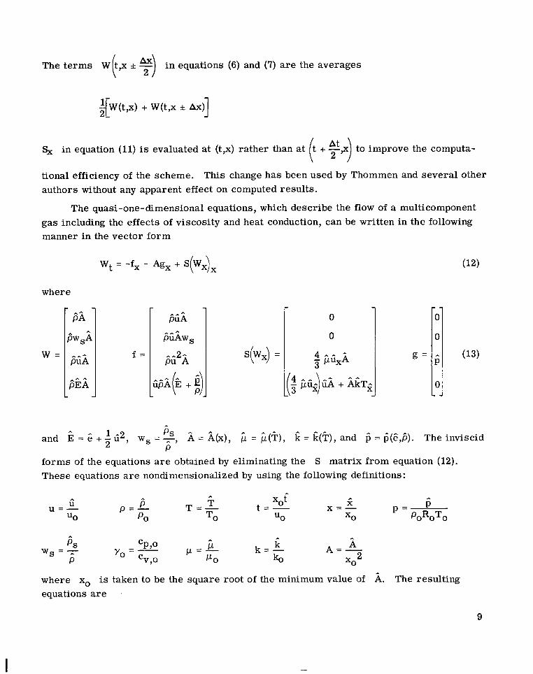
The te rms W (t,x f -2)in equations (6) and (7) a r e the averages

I[W(t,x) + W(t,x f Ax)12-

S, in equation (11)is evaluated at (t,x) rather than at t + -,x to improve the computa­( :) tional efficiency of the scheme. This change has been used by Thommen and several other authors without any apparent effect on computed results.

The quasi-one-dimensional equations, which describe the flow of a multicomponent gas including the effects of viscosity and heat conduction, can be written in the following manner in the vector form

W t = -f, - A9, + S(WX),

where

W = f = g =

A

and k = e + l d 2 , w S = -psA , A = 6(x), c = ;($, i; = G(?), and 5 = G(6,b). The inviscid2 P

forms of the equations a r e obtained by eliminating the S matrix from equation (12). These equations a r e nondimensionalized by using the following definitions:

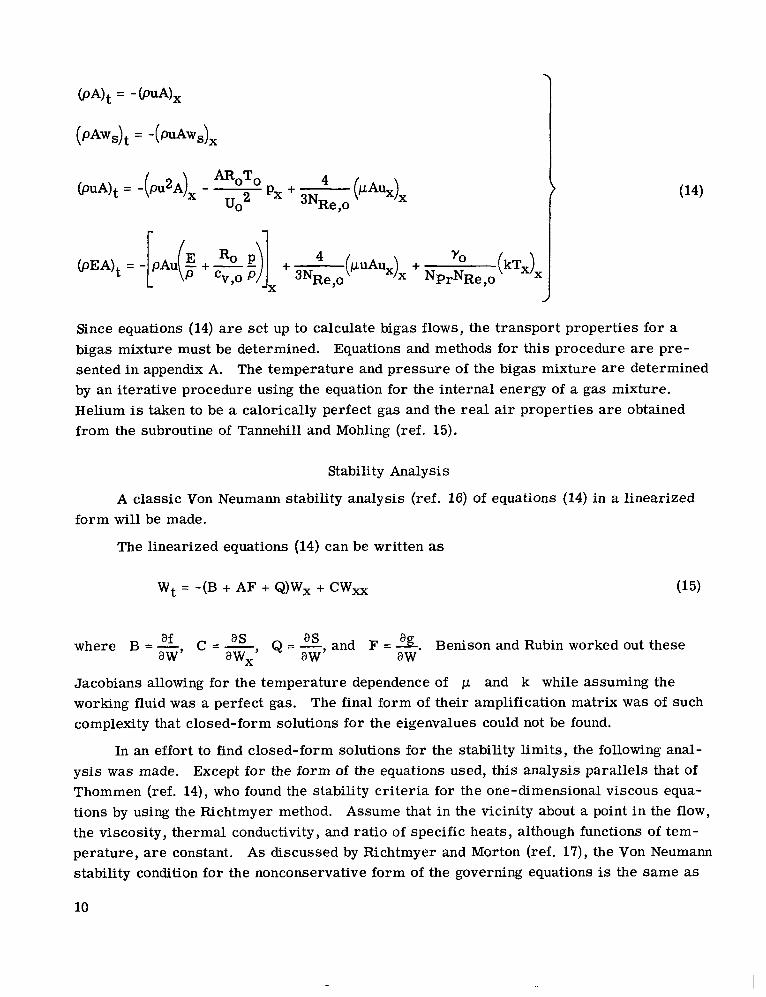
where xo is taken to be the square root of the minimum value of A. The resulting equations a r e .

9

r 1

Since equations (14)a r e set up to calculate bigas flows, the transport properties for a bigas mixture must be determined. Equations and methods for this procedure are pre­sented i n appendix A. The temperature and pressure of the bigas mixture are determined by an iterative procedure using the equation for the internal energy of a gas mixture. Helium is taken to be a calorically perfect gas and the rea l air properties a r e obtained from the subroutine of Tannehill and Mohling (ref. 15).

Stability Analysis

A classic Von Neumann stability analysis (ref. 16)of equations (14)in a linearized form will be made.

The linearized equations (14)can be written as

aw' c=-a w X

, Q = -,as and F = 3.Benison and Rubin worked out thesewhere B =-af a aw aw

Jacobians allowing for the temperature dependence of p and k while assuming the working fluid was a perfect gas. The final form of their amplification matrix was of such complexity that closed-form solutions for the eigenvalues could not be found.

In an effort to find closed-form solutions for the stability limits, the following anal­ysis was made. Except for the form of the equations used, this analysis parallels that of Thommen (ref. 14), who found the stability c r i te r ia for the one-dimensional viscous equa­tions by using the Richtmyer method. Assume that in the vicinity about a point in the flow, the viscosity, thermal conductivity, and ratio of specific heats, although functions of tem­perature, a r e constant. As discussed by Richtmyer and Morton (ref. l?),the Von NeumaM stability condition for the nonconservative form of the governing equations is the same as

10

--

--

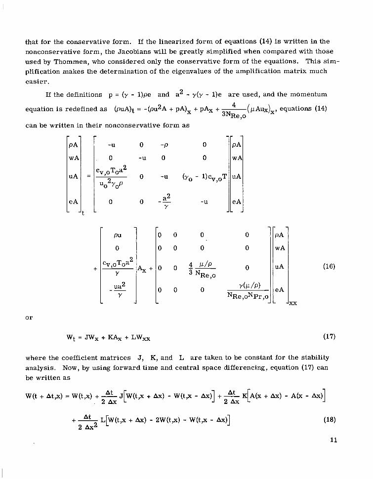
that for the conservative form. If the linearized form of equations (14) is written in the nonconservative form, the Jacobians will be greatly simplified when compared with those used by Thommen, who considered only the conservative form of the equations. This sim­plification makes the determination of the eigenvalues of the amplification matrix much easier.

If the definitions p = ( y - 1)pe and a2 - y(y - l)e are used, and the momentum

equations (14)equation is redefined as (puA)t = -(pu2A + PA), + pAx + 4 (~ A U ~ ) ~ ,3NRe ,O

can be written in their nonconservative form as - -

PA -U 0 -P 0 PA

wA 0 -U 0 0 wA

-'V,O T0a2 uA =

2 0 -U uA uo YOP

0 0 a2 -U eAeAJt Y -

PU

0 1 2

+ cv ,oToa A x +Y

Y . 1

o r

W t = Jwx + KAX + LW,,

0 0

0 0

4 P/P 0 NRe,o

0 Y(P/P) NRe,oNPr,o

PA

wA

uA

eA

. .

where the coefficient matrices J, K, and L are taken to be constant for the stability analysis. Now, by using forward time and central space differencing, equation (17) can be written as

W(t + At,x) = W(t,x) + -A t J[W(t,x + Ax) - W(t,x - Ax)] + -A t K[A(x + Ax) - A(x - h)] 2 A x 2 A x

+ -At L[W(t,x + Ax) - 2W(t,x) - W(t,x -4 2 Ax2

11

Following reference 18, assume W(t,x) is an exact solution of equation (18) and &,x) is the e r r o r in the solution at x and t. Then, substituting W(t,x) = W(t,x) + E(t,x) into equation (18) gives

W(t + At,x) + E ( t + At,x) = W(t,x) + E(t,X) + -A t J[W(t,x + Ax) + E(t,X + Ax) - W(t,x - Ax)2 A x

+ E(t,X + Ax) - 2W(t,x) - 2E(t,X) + W(t,x - Ax) - E(t,X - AX,] (19)

When equation (18) is subtracted from equation (19), an expression for the e r r o r at (t + At,x) is found, and the expression

E ( t + At,x) = E(t,X) + - + Ax) - E(t,x - Ax)] + L[�(t,X + Ax)2 A x 2 Ax2

- 2E(t,X) + E(t,X - Ax)1 is independent of the expression KA,. Therefore, only the stability of the expression

will be investigated.

For the inviscid case, equation (20) reduces to Wt = JW,, the stability criterion of which is established by the well-known C FL (Courant-Friedrich-Lewy) condition At/AX = l/(u + a).

Following Von Neumann, equation (20) is differenced according to the Richtmyer method. However, for the case of constant coefficients, the Richtmyer method reduces to the original Lax-Wendroff method; that is,

W(t + At,x) = W(t,x) + J[W(t,x + Ax) - W(t,x - Ax)] + 2 A x 2 Ax2

- 2W(t,x) + W(t,x - Ax)] +-:$ [Wxx(t,X + Ax) - W,(t,x - Ax)1 + L A t W,(t,x)

where higher order t e rms in L have been neglected.

12

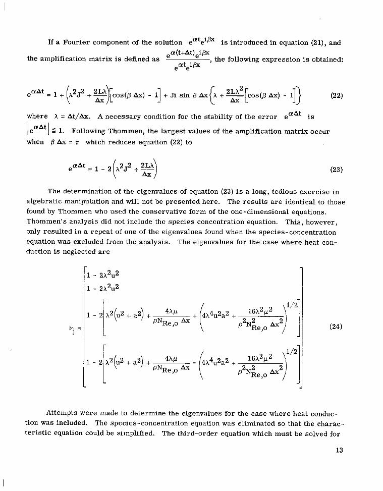
If a Fourier component of the solution ecuteipx is introduced in equation (21), and

the amplification matrix is defined as ecu (t+At)ei@ the following expression is obtained:

ecutei@

e hx) - 11 + Ji sin @ Ax

where X = At/&. A necessary condition for the stability of the e r r o r e@At is

lecuAt1 5 1. Following Thommen, the largest values of the amplification matrix occur when p Ax = 71 which reduces equation (22) to

The determination of the eigenvalues of equation (23) is a long, tedious exercise in algebratic manipulation and will not be presented here. The results are identical to those found by Thommen who used the conservative form of the one-dimensional equations. Thommen’s analysis did not include the species concentration equation. This, however, only resulted in a repeat of one of the eigenvalues found when the species-concentration equation was excluded from the analysis. The eigenvalues for the case where heat con­duction is neglected are

1 - 2h2u2 1 - 2 h u2 2

1 - 2,2(u2 + “2) + 4 h ~ + 4X4u2a2 + PNRe,o Ax (

L J

r

Attempts were made to determine the eigenvalues for the case where heat conduc­tion was included. The species-concentration equation was eliminated so that the charac­teristic equation could be simplified. The third-order equation which must be solved for

13

the eigenvalues is quite involved in this case. Therefore, the eigenvalues of the amplifi­cation matrix were found by using a symbolic manipulator computer code. The resulting answers are presented i n appendix B. One is real, the other two are complex. The max­imum eigenvalue will most likely come from one of the complex forms. Since the condi­tion for stability requires the magnitude of the eigenvalue to be less than one, it would be necessary to evaluate the roots of

lVj I 2 1 to find the appropriate value of A. It would

be preferable if such a calculation could be avoided by considering (1)the complexity of

, (2) the number of t imes l V j /

i5 1 would have to be evaluated, and (3) that an iterative l v j l

procedure would have to be used to determine A. Thommen (ref. 14) looked at the sta­bility of the equations in a quiescent region when heat conduction was included and found the stability criterion to be too restrictive. He obtained good results in subsequent cal­culations by basing the stability on the eigenvalues (eq. 24). Thus, the stability of the viscous equations will be based on the eigenvalues (eq. (24)).

Solution Stability

To test the computational scheme, a simplified test case was run for a nozzle having = 16.67 N/m2 in helium, a primary shock Mach number of 5, and no ternery

P@ =p@ diaphragm in the system.

Equations (14) were used in their inviscid form which resulted in a numerical insta­bility just upstream of the secondary starting shock. Figure 3 shows the evolvement, in

of the density for this test case.time, of the axial distributions of velocity and loglo The continuous upper and lower portions of the u/uo and loglo -P curves, respectively,

PO

represent the steady expansion solution for the nozzle. The position of the primary shock Inspection of the firstis indicated on the velocity curve for the first time interval shown.

curve shows no evidence of a secondary starting shock (SSS). The second curve shows a

steepening of the u/uo and loglo -P gradients near the steady expansion curve, while PO

the third curve indicates a definite shock a t the same point accompanied by a slight over­shoot in the velocity and density. As the SSS t raverses the nozzle, oscillations associated with the numerical solution appear at the upstream side of the shock. These ultimately cause a negative temperature to appear, leading to a rapid degeneration of the solution.

The instability in the solution did not seem to be related to the step size used, since the oscillations at the shock had appeared when it was first formed near the nozzle entrance and did not grow as the shock moved downstream. Only when the temperature at the shock, because of the highly expanded nature of the flow, became small when compared

14

I

with the oscillations in the temperature did the negative temperature and subsequent insta­bility occur. Since all second-order-accurate and higher order accurate difference schemes have oscillations a t a shock unless sufficient damping is provided (e.g., artifi­cial viscous t e rms used by Lava1 and others), the full viscous form of equations (14) was used to see if the rea l viscous effects would be sufficient to damp the oscillations a t the shock. This seemed to be a reasonable course to follow since the free-s t ream unit Reynolds numbers were small enough to allow cell Reynolds numbers in the range of 2 to 10.

Sufficient smoothing of the solution was accomplished by using the viscous form of equations (14) and a spatial increment small enough to permit resolution of the secondary starting shock. In this manner, satisfactory results were obtained, although some accu­racy had to be sacrificed as a result of the smearing of shocks and interfaces by the vis­cous effects. An example of these results is shown in figure 4. As the flow progresses through the nozzle, the shock is smeared out and the overshoot disappears. Note, how­ever , that the oscillations at the primary shock never disappear. The cause of this effect is readily apparent when the nonconservative equations (eqs. (17)) a r e examined. The coefficients of the Wxx te rms a r e made up in part by a te rm p/PNRe,o, which is, in

effect, an inverse unit Reynolds number based on the local f ree-s t ream density and vis­cosity and on the reference velocity. The value of this Reynolds number var ies widely along the nozzle as the solution evolves in time. Small values of the inverse Reynolds number force the equations to the hyperbolic limit, for which oscillations at discontinu­it ies a r e assured when second-order-accurate difference schemes are used. Large V a l ­

ues, on the other hand, maintain the parabolic character of the equations and smear out discontinuities if the spatial increment is sufficiently small to provide good resolution. Thus, for the case shown in figure 4, equations (14) a r e parabolic-dominant in the vicinity of the SSS and hyperbolic-dominant near the primary shock.

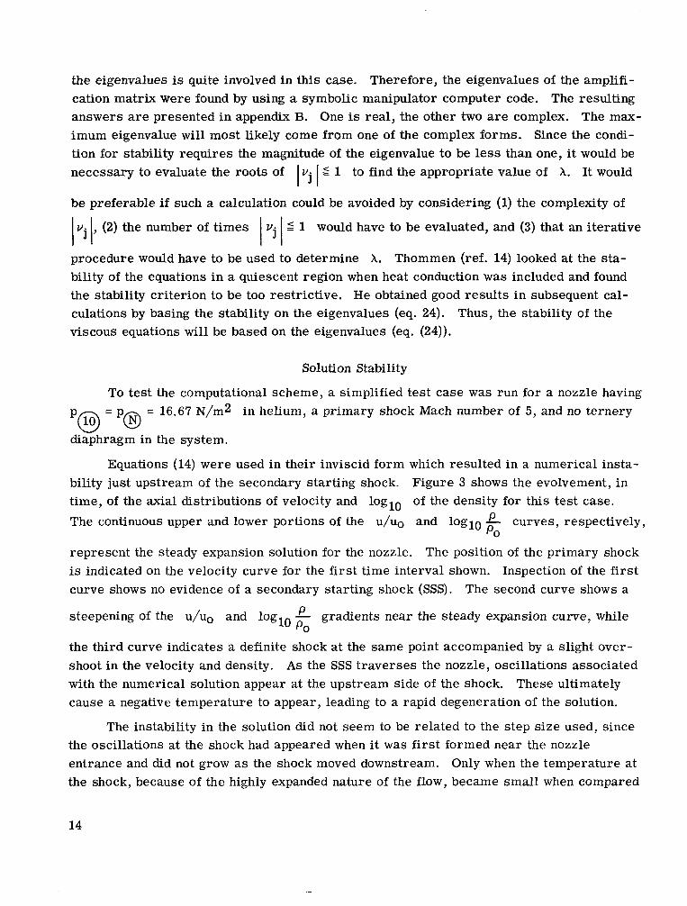
Although the use of the viscous form of the equations to stabilize the SSS worked well in this case, the very nature of expansion tube flow suggested that such a procedure would be incapable of handling the range of conditions required for this study. In refer­ence to the following sketch, the local Reynolds number in region @ is much l e s s (an

Time

A

-

Nozzle length

15

order of magnitude o r more) than the local Reynolds number in region 0.Thus there would be a large jump in the inverse Reynolds number across the interface. Initial cal­culations showed that i f the SSS followed path A, it would remain stable, whereas, if the shock followed path B and moved across the interface, the computation would destabilize at the SSS. This behavior is consistent with the previous observation of the effect of the local inverse Reynolds number (Le., cell Reynolds number) and its relation to the stability of the S S S .

Thus, to generate a general algorithm for this problem, it w a s necessary to intro­duce a stabilizer for the S S S . One option would have been to implement the stabilizers used by Richtmyer (ref. 16) or Lava1 (ref. 12),or to decrease the cell Reynolds number in the expanded gas of region @ by a corresponding reduction in grid size. Use of the

inviscid form of the equations along with the simple smoothing method proposed by Lapidus (ref. 19) appeared to be a more attractive option.

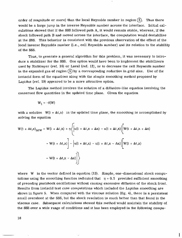
The Lapidus method involves the solution of a diffusion-like equation involving the conserved flow quantities in the updated time plane. Given the equation

W t = -f(W)

with a solution W(t + At,x) in the updated time plane, the smoothing is accomplished by solving the equation

W(t + At,x)new = W(t + At+) + + At,x + AX) - u(t + At,x) + At,x + AX)

- W(t + At,x)] - /u(t + At,x) - u(t + At,x - AX)

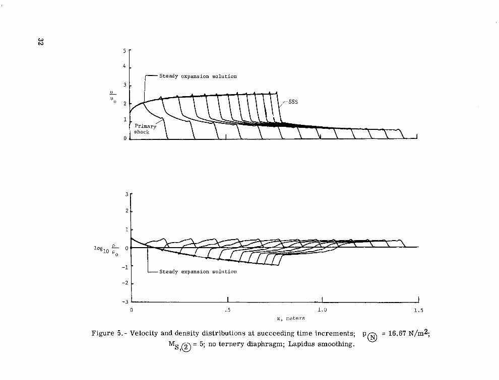
- W(t + At,x - AX)I> where W is the vector defined in equation (13). Simple, one-dimensional shock compu­tations using the smoothing function indicated that q = 0.5 provided sufficient smoothing of preceding postshock oscillations without causing excessive diffusion of the shock front. Results from inviscid test case computations which included the Lapidus smoothing are shown in figure 5. When compared with the viscous solution (fig. 4), there is a persistent small overshoot at the S S S , but the shock resolution is much better than that found in the viscous case. Subsequent calculations showed this method would maintain the stability of the SSS over a wide range of conditions and it has been employed in the following compu­

16

tations. Use of the Lapidus smoothing does not affect the stability cri terion for the numerical method which was taken to be the standard CFL condition for the inviscid form of equations (14).

RESULTS

Nonevacuated Nozzle

Inclusion of a ternery diaphragm in the expansion tunnel system is based on the assumption that to have acceptable nozzle s t a r t s , the nozzle would have to be at a much lower initial pressure than the acceleration chamber. Since operation of the facility would obviously be easier i f this diaphragm could be eliminated, the first cases were run to determine i f acceptable nozzle starts could be made when the nozzle pressure was the same as the acceleration chamber pressure.

Figure 5 shows data for a case where an initial shock Mach number was 5 at the nozzle entrance and where the arr ival of the interface separating the acceleration gas and test gas was not taken into account in the computation. In determining the conditions to be used for region 0,the pressure and velocity in regions @) and @ must be matched. The matching is done by finding simultaneous solutions for the Rankine-Hugoniot relations across the shock in the acceleration chamber and by finding the relationships governing the unsteady expansion of the flow from region@. Typical expansion tube conditions of 50 to r r in air in region @ and a shock Mach number of 7.93 in the intermediate chamber were used to obtain the conditions for region@. Matching the conditions required a shock of MS,@ = 7.95 moving into region 10 which had an initial pressure of 0.8860 t o r r in helium o r a shock of MS,@ = 16.59 moving into air at 0.360 to r r . The initial conditions and reference values used in these computations a r e in table 1. The time interval between shock and interface arr ival a t the nozzle entrance was taken from exper­imental results to be 50 p s and 20 p s for the helium and air acceleration gases, respectively.

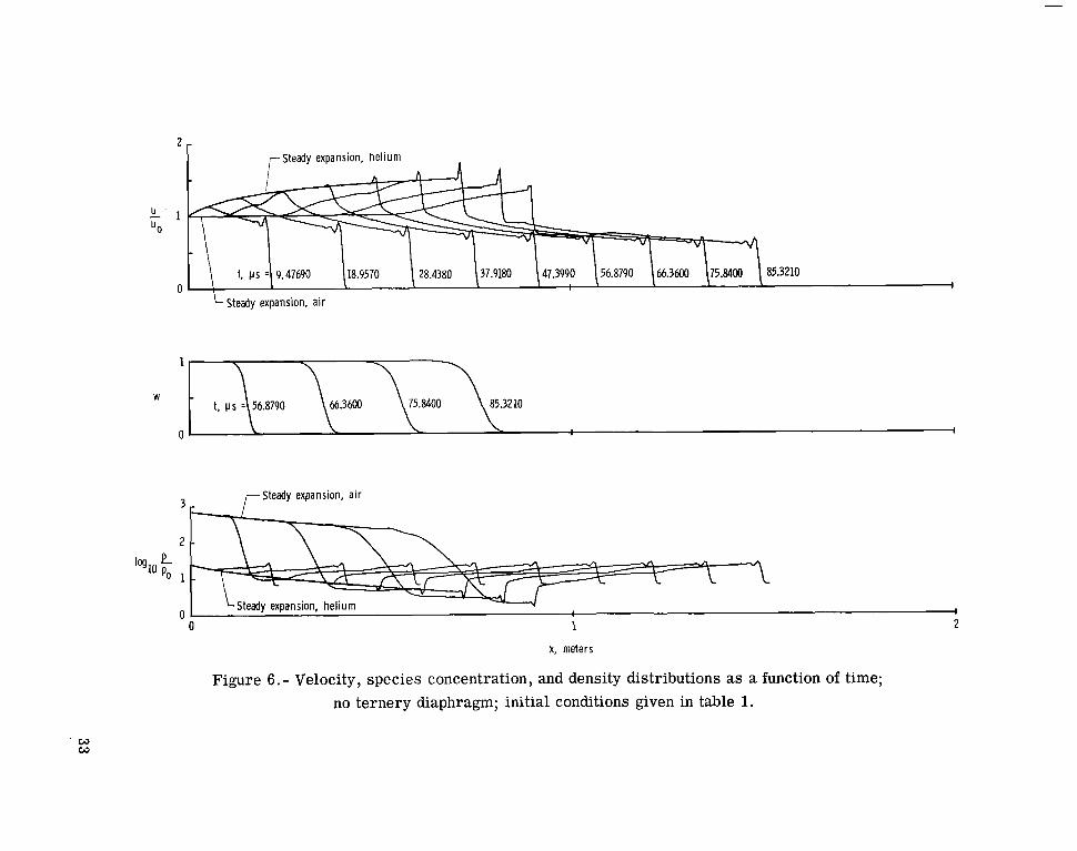
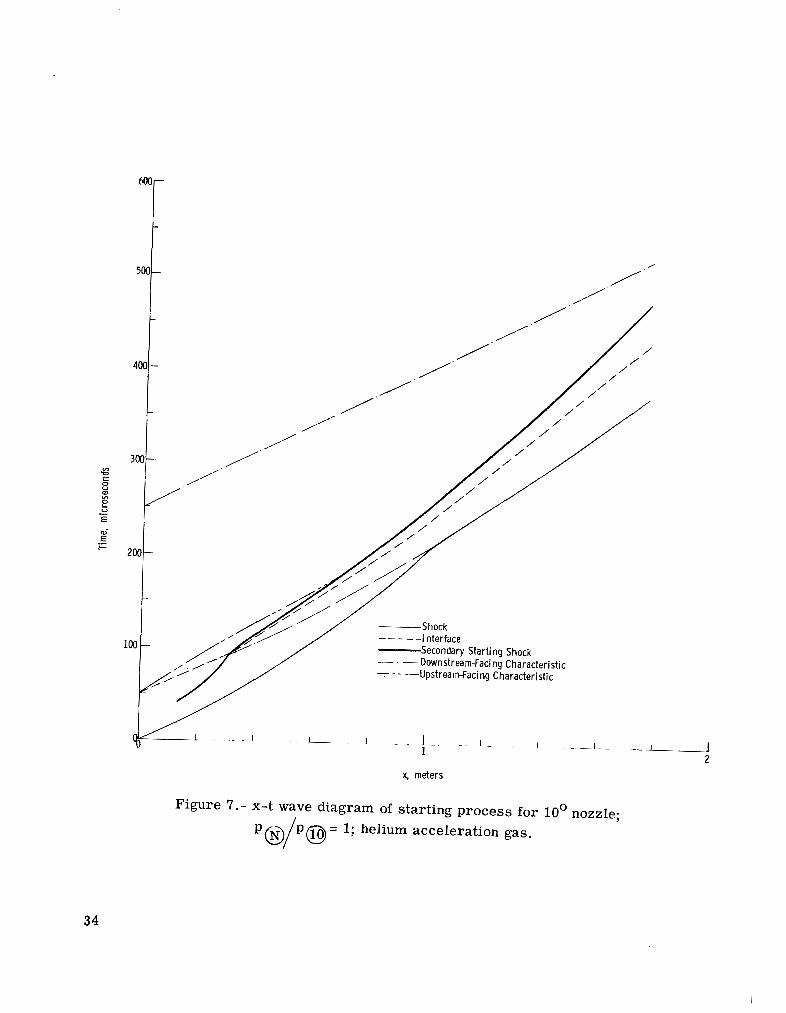
Figure 6 shows some partial resul ts for a loo nozzle and helium acceleration gas. Pertinent facets of the flow can be determined from such plots and transfered to x-t wave diagrams for more convenient comparison and analysis. Cases were also run for an 8' nozzle with a helium acceleration gas and a loo nozzle with an air acceleration gas. Results for these three cases are shown in figures 7, 8, and 9. In all three cases, the SSS gains strength quickly due to the large back pressure in the nozzle. After the SSS has passed through the interface, it is swept downstream at a more rapid rate because the free-stream Mach number of the test gas is greater than that of the acceleration gas. At approximately 0.6 m downstream of the diaphragm, the SSS and the trailing edge of the u-a family of starting waves intersect. After this intersection, the SSS moves downstream a t

17

a decreasing rate, thus affecting a portion of the test gas. In each case, substantial losses i n available test time are indicated at the la rger values of x.

This conclusion is in agreement with the experimental observations of Freisen and Moore (ref. 7), who found the test gas flow quality for nonternery diaphragm conditions to be very poor when compared with the flow observed when a ternery diaphragm, which results i n a lower nozzle pressure, was used.

Evacuated Nozzle

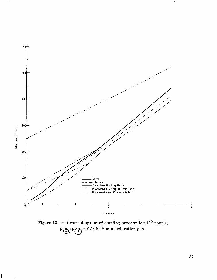
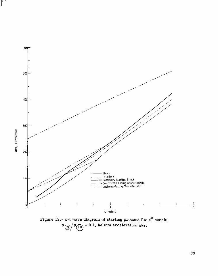
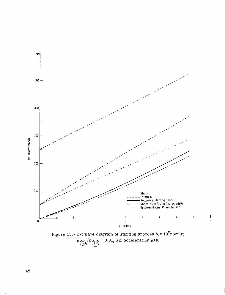
Inclusion of a ternery diaphragm in the system allows the initial nozzle pressure to be varied. A reduction in the value of p should lead to a reduced influence of the SSS0 on the test flow time. The three previous cases w e r e recomputed by using pressure ratios across the ternery diaphragm p@/P@

of 0.1 and 0.01. The resulting x-t

diagrams (figs. 10 to 15) show that in each case, subsequent reductions in p@k@ led to reductions in test-time losses.

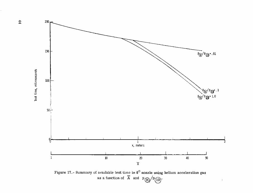
The effect of po/,@ on the available test time is summarized in figures 16

to 18 for each of the three cases. For both the 8O and 10' cases with helium as an accel­

eration gas, p a p @ of approximately 0.01 is needed to eliminate the effects of the

of only 0.1 is needed when air is used asSSS on the test gas flow, whereas a p@p@the acceleration gas.

The time of 200 ps between the a r r iva l of the interface and the expansion fan a t the nozzle entrance is based on experimental observations. Theoretically, this time could be increased by lengthening the acceleration chamber, thus decreasing the effect of the SSS on the available test time. However, viscous effects, as detailed in reference 20, degrade the quality of the flow in region @ after i t has traveled a sufficient distance downstream

of the secondary diaphragm. The 200 ps of test t ime used in this case is near the maxi­mum amount of good quality test flow that might be expected for these flow conditions.

Practical test setups require a balance between test time, test Mach number, and model size. Also, in this case, one of the factors in testing frequency is the ratio

P@/P@ . For some running conditions, P@ is very small; the facility configuration

is such that the volume of the nozzle and dump tank is very large, which for small values of p a leads to long nozzle evacuation times. To evaluate these effects for the data

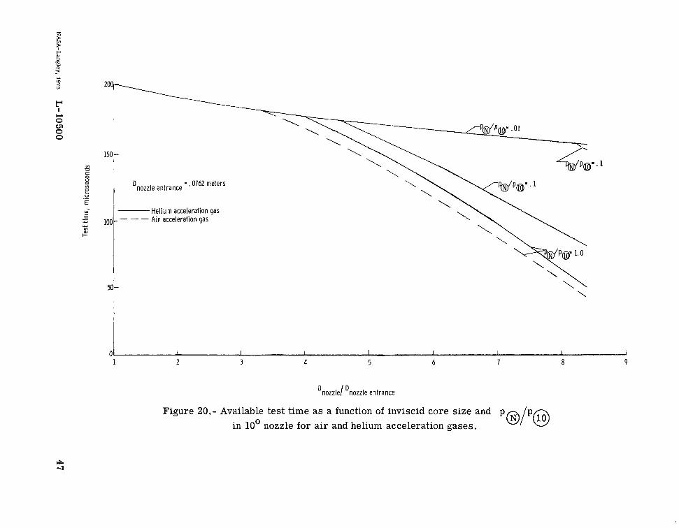
which have been presented, a plot of test time against exit Mach number is shown in fig­ure 19 and a plot of test time against model diameter, based on the nozzle entrance diam­eter , is shown in figure 20. The test flow Mach number can be doubled and a model size four times the nozzle entrance diameter is available i n a system which excludes a ternery

18

diaphragm without suffering SSS-related test-time losses. Further increases in exit Mach number and/or model size will result i n drastic reductions in available test time. This is also the case when a ternery diaphragm is used with helium acceleration gas and when

p a p @ = 0.1 is used for either nozzle configuration. Test flows are not free of inter­

ference from the SSS until p = 0.1 is used with air acceleration gas o r until

= 0.01 is used with a helium acceleration gas.p a p @

CONCLUDING REMARKS

A finite-difference solution of the time-dependent, quasi-one-dimensional equations for a bigas mixture, including real gas effects, for both viscous and inviscid flow has been applied to the starting process in an expansion tunnel nozzle.

An analysis of the numerical technique has shown that using a Richtmyer differencing solution of the inviscid quasi-one-dimensional equations along with a smoothing function avoids numerical instabilities unrelated to classical stability c r i te r ia and that the stability restriction on step size for the quasi-one-dimensional equations is identical to that for the one-dimensional equations.

The solutions obtained for the starting process in 8 O and loo conical nozzles having an entrance diameter of 0.076 m and a length of 1.609 m show that expansion tunnel oper­ation without a ternery diaphragm is limited to moderate Mach number test flows (Mach number of 12 to 13) and small area ratios (for example, small model diameters). The solutions also indicate that the use of a ternery diaphragm and ternery diaphragm pres­su re ratios of 0.1 and 0.01 for air and helium acceleration gases, respectively, allows the full potential of the nozzle to be realized (that is, expansion to a Mach number of about 18 in the nozzles with an area ratio of 70).

Langley Research Center National Aeronautics and Space Administration Hampton, Va. 23665 November 14, 1975

19

APPENDIX A

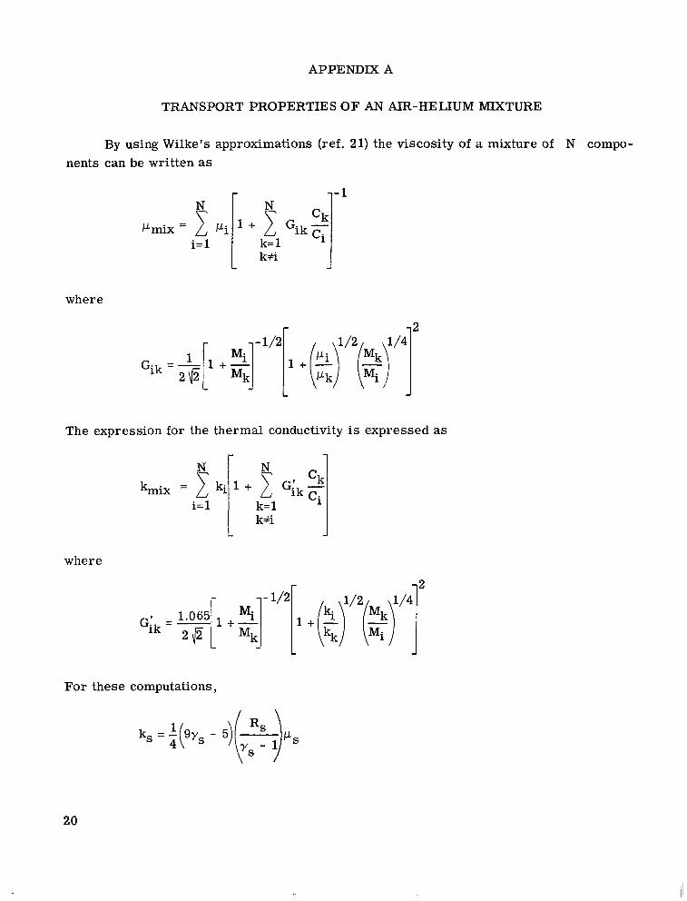
TRANSPORT PROPERTIES OF AN AIR-HELIUM MIXTURE

By using Wilke's approximations (ref. 21) the viscosity of a mixture of N compo­nents can be written as

r 1-1 N N

IJ.mix = 2 pi '+1G i k qck i=1 k=11 k t i J

where

The expr sion for the thermal conductivity is expressed S

r 1

1 kfi

where

I- 2

L

For these computations,

20

APPENDIX A

The expression for the viscosity of helium is broken up into two temperature ranges. For T < 1000 K,

pHe = 2.3479 X 10' 7 T 0.647

and for T 2 1000 K,

pHe = 1.6215 X + 1.02085X T - 8.33348X T2 + 7.5447X 1O-l' T3

which is a curve fit of the data of Amdur and Mason (ref. 22).

For temperatures less than 3000 K,the viscosity of air is taken from Hansen T3/2

(ref. 23)as 8.1363 x (T + 363.6)' For temperatures greater than 3400 K and l e s s

than 15 000 K,interpolation from Hansen's tables of p = p(T,p) is used to determine the viscosity.

21

--

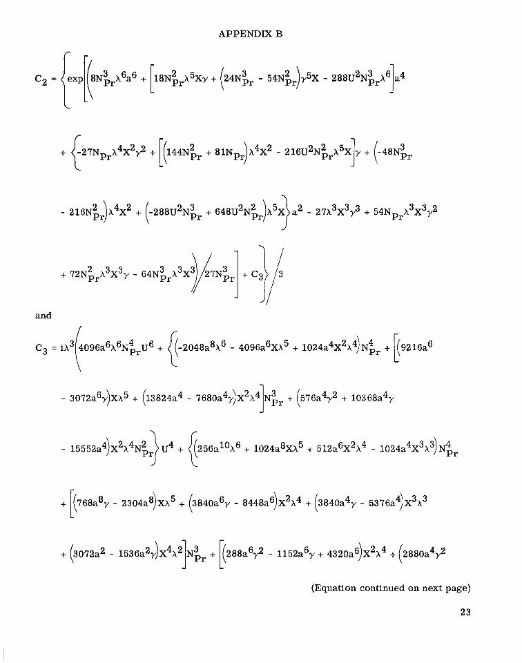
APPENDIX B

COMPUTED EIGENVALUES

The computed eigenvalues for the case where heat conduction is considered are as follows:

X -Npr + 4XXNpr - 3Np,_-+ 3 y x ~ iF(c2 - ~ 1 )~2 + ~1V I = - 6X2NprU 2 + 4a2 2 -

3 N ~ r 2 2

6X2NprU 2 + 4a2 2X Npr + 4XXNpr - 3Npr + ~ Y X X i P ( c 2 - ~ 1 )~2 + ~1 v2 = +

3Npr 2 2

6X2NprU 2 + 4a2X2Npr + 4XXNpr - 3Npr + 3yXX .__ .- + c2 + c1

”3 = - 3Npr

where X = 4p/3NprN~,, ,

3+ (24Npr - 54N2p,)h5X - 288U

144N& + A4X2 - 216U2N:rA5X]? + (-48Nir

- 216Npr X X2 ) 4 2 + (-288U2Nir + 648U2N$:lh53a2 - 2 7 ~ 3 x ” y 3+ 54NprX3X3y2

+ 72Nirh3X3y - 64Nirh3X3)/27Nir] - C j /

22

APPENDIX B

-

c2 = - 54N;I)y5X - 288U -

2+ [(l44NPr + 81Npr)X4X2 - 216U2Nirh5X]y + (-48Nir

b

y y+ 648U a2 - 27X3X3 3 + 54NprX 3X3 2

+ 72Nprh 3 32 X y - 64N;,X3Xy7N$,] + Ci/

and

- 4096a6Xh 5 + 1024a4X2X4)N$, + [(9216a6

- 3072a6y)Xh5 + (13824a4 - 7680a4y X2X4 N;, + 576a4y2 + 10368a4y) I (

256al0A6 + 1024a8XX5 + 512a6X2X4 - 1024a4 3 3 4X X)Np,

+ [(768a8y - - 8448a6)X2h4 + (3840a4y - 5376a)X3 34 X

) 4 2 3+ (3072a2 - 1536a2yX X ]Npr + [(288a6y2 - 1152a6y + 4320a6)X2h4 + (2880a4y2

(Equation continued on next page)

23

APPENDIX B

- 6336a4y + - 3456a2y)X h'1 Npr + [(-432a4y3 + 864a4y2

- 3888a4y)X3h3 + (-864a2y3 - 2592a2y 2) X4X 2 jNpr + 1296a2y3X4X2}U2 + (64a 8 2 4X h

+ 256a6X3X3 + 256a X X")Npr + [(96a8 - 9 6 a 8 y ) ~ 2 ~ 4+ (-192a6y - 192a6)x3k3

+ (384a4y - 1536a4)x4h2 + (768a2y - 1536a2)X5X]Nir + [(36a8y2 - 72a8y + 3 6 a ) X2 48 X

+ (-144a6y2 + 720a6y - 576a6)X3A3 + (-864a4y2 + 2880a4y - 1 1 5 2 a 4 ) ~ 4 ~ 2+ (2304a2y

- 576a2y2)X5h + 5763.2X'1 Npr + [(108ai6y3 - 432a6y2 + 540a6y - 216a6)x3h3

+ (216a4y3 - 1080a4y2 + 864a4y)X4h2 + (-432a2y3 - 432a2y2)x5~- 864y3X6]Npr

81a4y4 - 162a4y3 + 81a4y2)X4h2 + (324a2y4 - 324a2 3y )X 5X + 324y

24

d

REFERENCES

1. Weilmuenster, K. James: A Finite -Difference Solution for Unsteady Wave Inter­actions With an Application to the Expansion Tube. Recent Developments in Shock Tube Research, Daniel Bershader and Wayland Griffith, eds., Stanford Univ. Press, 1973, pp. 534-545.

2. Trimpi, Robert L.: A Preliminary Theoretical Study of the Expansion Tube, A New Device for Producing High-Enthalpy Short-Duration Hypersonic Gas Flows. NASA TR R-133, 1962.

33. Jones, J. J.: Some Performance Characteristics of the LRC 3--Inch Pilot Model4Expansion Tube Using an Unheated Hydrogen Driver. Fourth Hypervelocity Tech ­niques Symposium, Univ. of Denver and Arnold Eng. Develop. Center, Nov. 1965, pp. 7-26.

4. Jones, J i m J.; and Moore, John A.: Exploratory Study of Performance of the Langley Pilot Model Expansion Tube With a Hydrogen Driver. NASA TN D-3421, 1966.

5. Trimpi, Robert L.; and Callis, Linwood B.: A Perfect-Gas Analysis of the Expansion Tunnel, A Modification to the Expansion Tube. NASA TR R-223, 1965.

6. Glick, H. S.; Hertzberg, A.; and Smith, W. E. : Flow Phenomena in Starting a Hyper­sonic Shock Tunnel. AEDC-TN-55-16 (AD-789-A-3), U. S. Air Force, Mar. 1955.

7. Friesen, Wilfred J.; and Moore, John A.: Pilot Model Expansion Tunnel Test Flow Properties Obtained From Velocity, P res su re , and Probe Measurements. NASA TN D-7310, 1973.

8. Weilmuenster, K. J.: A Self-opening Diaphragm for Expansion Tubes and Expansion Tunnels. AIAA J. , vol. 8, no. 3, Mar. 1970, pp. 573-574.

9. Smith, C. Pdward: The Starting Process in a Hypersonic Nozzle. J . Fluid Mech., vol. 24, pt. 4, Apr. 1966, pp. 625-640.

10. Stalker, R. J.; and Mudford, N. R.: Starting Process in the Nozzle of a Nonreflected Shock Tunnel. AIAA J. , vol. II, no. 3, Mar. 1973, pp. 265-266.

11. Crocco, L.: Solving Numerically the Navier-Stokes Equations. Doc. No. 63SD891 (Contract AF 04(694)-222), Re-Entry Syst. Dep., Gen. Elec. Co., Mar. 20, 1964. (Available from DDC as AD 439 220.)

12. Laval, Pierre: Pseudo-Viscosity Method and Starting Process in a Nozzle. NASA TT F-12,863, 1970.

13. Benison, G. I.; and Rubin, E . L.: A Time-Dependent Analysis for Quasi-One-Dimensional, Viscous ,Heat Conducting, Compressible Laval Nozzle Flows. J. Eng. Math., vol. 5, no. 1, Jan. 1971, pp. 39-49.

25

14. Thommen, Hans U.: Numerical Integration of the Navier -Stokes Equations. Z. Angew. Math. Phys., vol. 17, no. 3, 1966, pp. 369-384.

15. Tannehill, J. C.; and Mohling, R. A.: Development of Equilibrium Air Computer Programs Suitable for Numerical Computation Using Time -Dependent o r Shock-Capturing Methods. NASA CR-2134, 1972.

16. Richtmyer, Robert D.: Difference Methods for Initial-Value Problems. Interscience Publ., Inc., 1957.

17. Richtmyer, Robert D.; and Morton, K. W.: Difference Methods for Initial-Value Prob­lems. Second ed. Interscience Publ., c. 1967.

18. 0'Brien, George G.; Hyman, Morton A.; and Kaplan, Sidney: A Study of the Numerical Solution of Partial Differential Equations. J. Math. Phys., vol. 29, no. 4, Jan. 1951, pp. 223-251.

19. Lapidus ,Arnold: A Detached Shock Calculation by Second-Order Finite Differences. J. Comput. Phys., vol. 2, no. 2, Nov. 1967, pp. 154-177.

20. Weilmuenster ,K. James: An Experimental Investigation of Wall Boundary -Layer Transition Reynolds Numbers in an Expansion Tube. NASA TN D-7541, 1974.

21. Wilke, C. R.: A Viscosity Equation for Gas Mixtures. J. Chem. Phys., vol. 18, no. 4, Apr. 1950, pp. 517-519.

22. Amdur, I.; and Mason, E . A.: Properties of Gases at Very High Temperatures. Phys. Fluids, vol. 1, no. 5, Sept-Oct. 1958, pp. 370-383.

23. Hansen, C . Frederick: Approximations for the Thermodynamic and Transport Prop­er t ies of High-Temperature Air. NASA TR R-50, 1959. (Supersedes NACA TN 4150.)

26

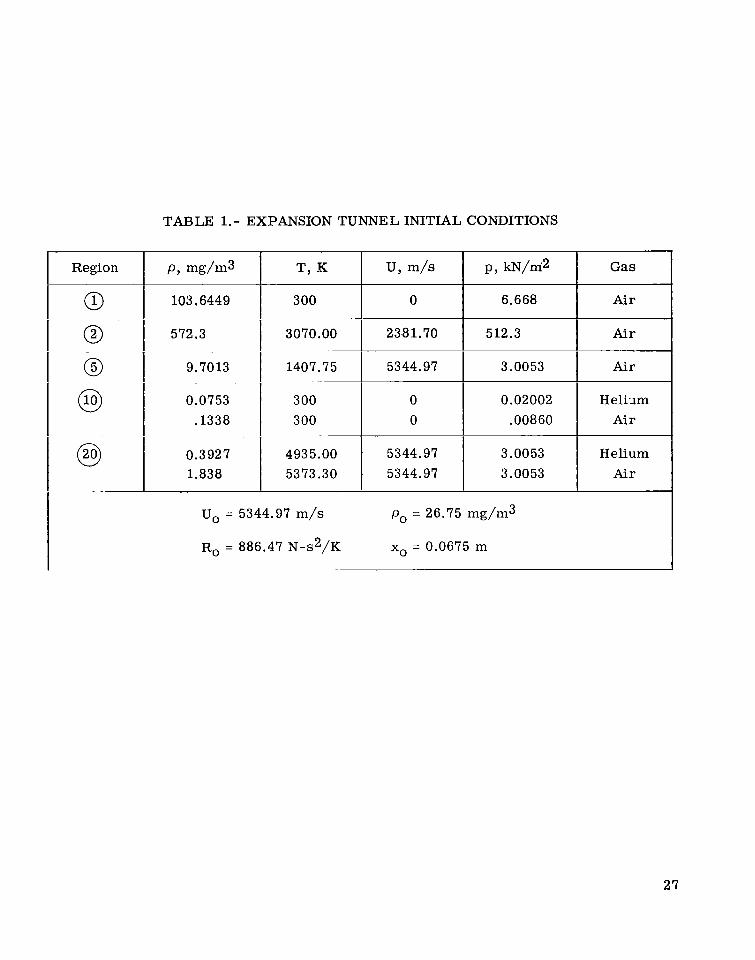
TABLE 1.- EXPANSION TUNNEL INITIAL CONDITIONS

U, m/s I p, kN/m2 I Gas

103.6449 I 300 0 I 6.668 I Air

572.3 3070.00 2381.70 I 512.3 I Air ~

9.7013 1407.75 5344.97 I 3.0053 I Air ~ ~~

0.0753 300 0 0.02002 H eli-lm .1338 300 0 .00860 Air

~ ~~ . .

0.3927 4935.00 5344.97 3.0053 Helium 1.838 5373.30 5344.97 3.0053 Air

U, = 5344.97 m/s p, = 26.75 mg/m3

R, = 886.47 N-s2/K x, = 0.0675 m

27

I

Drive r intemediatf chamber I Acce le ra t ing chamber

-

Pr imary Secondary Temery diaphragm diaphragm diaphragm

,,,+-., Shock wave - - - - Part ic le pa th ___ C h a r a c t e r i s t i c s

f 0 /

,./’

Dis tance , x

Figure 1.- Schematic and wave diagram for expansion tunnel.

28

t

Air-helium interface

I X

Nozzle Nozzle exitentrance

Figure 2. - Wave diagram, imperfect nozzle start.

29

Primary Shock

x, meters

Figure 3. - Velocity and density distributions a t succeeding time increments;

P@ = 16.67 N/m2; Ms,@ = 5; no ternery diaphragm; inviscid case.

30

I ,Steady expansion solution

3 ­

2 I-

EOloglo Po

-1

-2 h e a d y expansion solution

I I I

x, meters

Figure 4.- Velocity and density distributions at succeeding time increments; p a = 16.67 N/m2;

MS ,.a= 5; no ternery diaphragm; viscous case,

w CL

I

I

Steady expansion s o l u t i o nl t r U L

U 0 2

1

0

3

1I/ - I Steady expansion s o l u t i o n

- 2 t -

0 5 1.0 1.5 x, meters

Figure 5. - Velocity and density distributions at succeeding time increments; p a = 16.67 N/m2; MS ,a5; no ternery diaphragm; Lapidus smoothing.=

21. r Steady expansion, helium

Steady expansion, ai r

1

W

0 I

3 - r Steady expansion, air

0 Steady expansion, helium I

0 1 2

x, meters

Figure 6. - Velocity, species concentration, and density distributions as a function of time; no ternery diaphragm; initial conditions given in table 1.

w w

/’/

/ ’/

” /

x, meters

Figure 7.- x-t wave diagram of starting process for 10’ nozzle;

= 1; helium acceleration gas.

34

/ - Shock - - - _Inter face

-Secondary Start ing Shock -. -Downstream-Facing Characterist ic

-Upstream-Facing Characterist ic

I I I I 1 I I I .I 1 2

x, meters

Figure 8.- x-t wave diagram of starting process for 8°nozzle; p a / p@ = 1; helium acceleration gas.

35

___Shock

/

//-//

/'/

//

/ a­.-E c

200 _1111/13;

lOD/ // ----- In te r face

-Secondary Start ing Shock // -. --Downstream-Facinq Characterist ic

I I 1 2

x. meters

0Figure 9.- x-t wave diagram of starting process for 10 nozzle;

P@/P@ = 1; air acceleration gas.

36

W

400cI

I /"

VI'CIlz 0u VI

e .-U

E

-Secondary Star t ing Shock Downstream-Facing Character is t ic

-Upstr ea m-Faci n g Character is t ic

I I . I 1 I I 1 I ' -*1

4 meters

Figure 10.- x-t wave diagram of starting process fo r 10' nozzle; = 0.1; helium acceleration gas.

37

T

t I’

// -Shock _ _ _ _ _Inter face -Secondary S tar t ing Shock

Downstream-Facing Character ist ic -_ --4Jpstream-Facing Character ist ic

I .I . I _LA- I I I I oo- 1

x. meters

Figure 11.-x-t wave diagram of starting process for 10’ nozzle; p a / p @ = 0.01; helium acceleration gas.

J 2

38

P

//

x, meters

Figure 12.- x-t wave diagram of starting process for 8' nozzle; p a l p @ = 0.1; helium acceleration gas.

39

'EI

6M

500

400

300 YI

s 0)* z U

1-

E

E i= 200

100

0

x, meters

Figure 13.- x-t wave diagram of starting process for 8' nozzle; = 0.01; helium acceleration gas.

40

c

0)

v)vc 0 U v)

e.-u E

~ Shock _ _ _ _ Inter face -Secondary Start ing Shock - . -Downstreamfac ing Characterist ic -Upstream-Facing Characterist ic

I I 1 I I I - ____ I 0 1 2

x. meters

Figure 14.- x-t wave diagram of starting process for 10' nozzle; = 0.1; air acceleration gas.

41

V

L

50(

4oc

300 mc

8 aIA0u .-E

.-E­200

100

0 1 x. meters

Figure 15.- x-t wave diagram of starting process for loonozzle; " @ / p a = 0.01; air acceleration gas.

1 I 2

42

Figure 16.- Summary of available test time in 10' nozzle using helium acceleration gas-

as a function of and p

2

a

c

2M

v)U c 0V v)

2 10 .-V

E a­.-� c

v) P@/P@= 1.0 a i­

5

1 2 x, meters

1 10 20 30 40 50 -A

Figure 17.- Summary of available test time in 8' nozzle using helium acceleration gas as afunction of and p

W

20(

15(

VI U C s VI

e lo(.-V

E

.-E­c

5 c

I I I I

0

VI

-1%

VI U c V

.-I

I

W I c I

I

1 i

I

I

O J 7

6 - ioo, h e l i u m acce le ra t i on gas

6 - loo, air acce le ra t i on gas

-.- 6 - So, helium acce le ra t i on gas

I I I I I I I I I I 1 I I 8 9 10 11 12 13 14 15 16 17 18 19 20

MACH NUMBER

Figure 19.- Available test time as a function of exit Mach number and p

r

/-PdPm= .01

150-I

- .0762 metersDnozzle entrance

Helium acceleration gas loo-- --A i r acceleration gas

! I

M \

DDnozzle/ nozzle entrance

Figure 20.- Available test time as a function of inviscid core size and p in 10' nozzle for air and helium acceleration gases.

NATIONAL AERONAUTICS A N D S P A C E ADMINISTRATION WASHINGTON, D.C. 20546

OFFICIAL B U S I N E S S PENALTY FOR PRIVATE USE s300 SPECIAL FOURTH-CLASS R A T E

BOOK +

f j ! C 1 7 U1 U C I 3 1 Z 1 L Sf,‘3Yl3JDS 9FPT OF THE PI3 PCSCE AP WEAPCES L A B C R A T O F Y BT’IN: T E C H N I C 9 L L I R F A F Y ( S O L ) K I R T L A N C A F B N Y 87117

POSTAGE A N D FEES P A I D N A T I O N A L AERONAUTICS A N 0

SPACE A D M I N I S T R A T I O N 451

USMAIL -U

: If Undeliverable (Section 158 Postal Mnnual) Do Not Return

,,.

“The aeronautical and space activities of the United States shall be conducted so as to contribute . . . to the expansion of human knowl­edge of phenomena in the atmosphere and space. T h e Administration shall provide for the wzdest practicable and appropriate dissemination of information concerning its activities and the results thereof.”

I -NATIONAL AERONAUTICSAND SPACEACT OF 1958 . . 4 .

NASA SCIENTIFIC AND TECHNICAL PUBLICATIONS TECHNICAL REPORTS: Scientific and ,

. technical information considered important, ..”. complete, and a lasting contribution to existing ’, . knowledge.

TECHNICAL NOTES: Information less broad in scope but nevertheless of importance as a contribution to existing knowledge.

TECHNICAL MEMORANDUMS: Information receiving limited distribution because of preliminary data, security classifica­tion, or other reasons. Also includes conference proceedings with either limited or unlimited distribution. -CONTRACTOR REPORTS: Scientific and technical information generated urider a NASA contract or grant and considered an important contribution to existing knowledge.

TECHNICAL TRANSLATIONS: Information published in a foreign language considered to merit NASA distribution in English.

SPECIAL PUBLICATIONS: Information derived from or of value to NASA activities. Publications include final reports of major projects, monographs, data compilations, handbooks, sourcebooks, and special bibliographies.

TECHNOLOGY UTILIZATION PUBLICATIONS : Information on technology used by NASA that may be of particular interest in commercial and other-non-aerospace applications. Publications include Tech Briefs, TechnoIogy Utilization Reports and Technology Surveys.

Derails on the availability of these publications may be obtained from:

. SCIENTIFIC AND TECHNICAL INFORMATION OFFICE

N A T I O N A L A E R O N A U T I C S A N D SPACE A D M I N I S T R A T I O N Washington, D.C. 20546

I