nasa-cr-194193 release date '3 low altitude plume ... · low altitude plume impingement...
TRANSCRIPT

NASA-CR-194193SECA-TR-91-8
RELEASE DATE___, _'3
LOW ALTITUDE PLUME IMPINGEMENT HANDBOOK
Contract No. NAS8-38423
Purchase Orders 1504, 1575, 1633, 1688, and 1808
"0//_ , " *
i/ i_ ..... "
Prepared for: i_ ""
REMTECH, Incorporated3304 Westmill Drive
Huntsville, AL 35805
I "" _
O" CZ _ 0
t'('l
0
By : uJ
Sheldon D. Smith D
_o
mzco_
SECA, Inc. J I', 3311 Bob Wallace Avenue
Suite 203 _ zuJ
Huntsville, AL 35805 _ x
August 9, 1991 _ z
I <_e[ Z-J_"
https://ntrs.nasa.gov/search.jsp?R=19940010268 2019-02-28T18:23:05+00:00Z
SECA-TR-91-8
Contents
List of Figures ............................................ ii: List of Tables ............................................ iii
NOMENCLATURE ........................................ iv1 INTRODUCTION ......................................... 12 BACKGROUND ......................................... 23 LOW ALTITUDE PLUME/PLUME IMPINGEMENT MODELING ............ 8
3.1 Free Exhaust Flowfield .................................. 83.2 Flat Plate Flow ...................................... 12
3.3 Heat-Transfer Analysis ................................. 124 LEVEL II IMPINGEMENTANALYSIS ........................... 15
4.1 SPF/2/and PLIMP Models 15
4.2 Application of the SPF/2/PLIMP Calculation for the TomahawkLC39 Simulations .................................... 20
4.3 Sample Problem Using SPF/2/PLIMP Level II Analysis ............. 234.4 Description of a Low Altitude Plume/Thermal Response Model ........ 23
4.4.1 Plume Flowfield ................................... 23
4.4.2 Impingement Flowfield 284.4.3 Convective Heating Rates 344.4.4 Thermal Model .................................... 40
5 LEVEL III LOW ALTITUDE IMPINGEMENTANALYSIS ................ 476 REFERENCES ......................................... 49

SECA-TR-91-8
List of Figures1 Space ShuttleSolidRocket Motor ExhaustPlumeCenterlinePitotTotal
PressureDistributionat Sea Level ............................... 32 Schematicof SPF/2 Gas�ParticleOvedaidProcedure................... 63 CentedineRecoveryPressures................................. 94 MK104 DTRM, TotalTemperatureComparison,Centerline,22% Aluminum.... 105 MixingRegionModel ...................................... 106 MK104 DTRM, PitotPressureComparison,X=40 Ft, 22% Aluminum........ 117 MK104 DTRM, TotalTemperatureComparison,X=55 Ft, 22% Aluminum ..... 118 Flow Regionfor Flat Plate Heat Transfer.......................... 129 CenteriineHeat FluxComparison .............................. 1310 AluminizedSolid-PropellantHeat Flux........................... 1411 Comparisonof Experimentaland CalculatedImpingementPressureDistribution
on Flat Plate 12.2 Ft from Exit Plane of TomahawkMotor .............. 2112 Comparisonof Experimentaland CalculatedImpingementPressureDistribution
on Flat Plate 17.0 Ft from Exit Plane of TomahawkMotor .............. 2213 Comparisonof 12.2 Ft Data and 17 Ft Data ....................... 2714 Space ShuttleSRM Radial Distributionsof Mach Number .............. 2915 Sea LevelSpace ShuttleSRM Radial PitotTotalPressureDistribution...... 3016 Space Shuttle SRM Radial Gas Recovery Temperature Distributions ....... 3117 Space Shuttle SRM Radial Distributions of Undisturbed Plume Particle
Mass Flux ............................................ 3218 Space Shuttle SRM Radial Distributions of Undisturbed Plume Particle
Total Energy .......................................... 3319 Space Shuttle SRM Ratio of Incident Particle Mass Flux to Undisturbed Plume
Particle Mass Flux as a Function of Local Plume Mach Number and ImpingedBody Effective Radius of Curvature ............................ 35
20 Space Shuttle SRM Ratio of Incident Particle Total Energy Flux to UndisturbedPlume Particle Total Energy Flux as a Function of Local Plume Mach Numberand Impinged Body Effective Radius of Curvature ................... 36
21 Effective Radius of Curvature of an Infinite Flat Plate Impinged upon by theSpace Shuttle SRM ...................................... 37
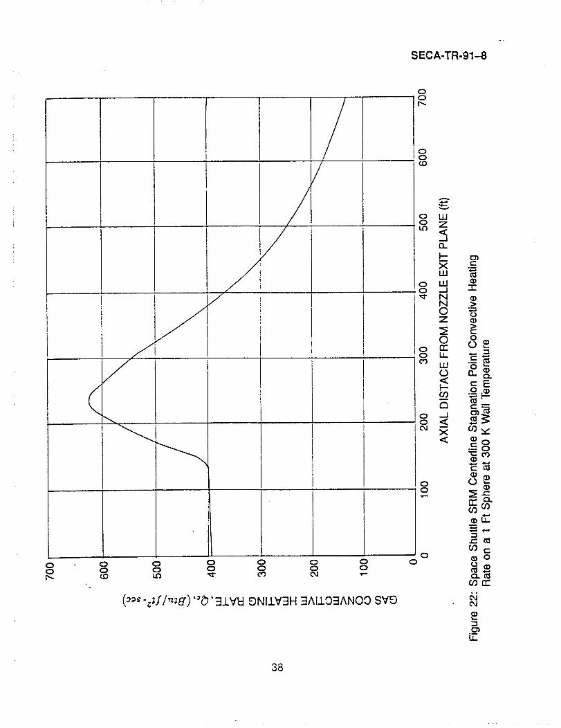
22 Space Shuttle SRM Centerline Stagnation Point Convective Heating Rate on a 1Ft Sphere at 300 K Wall Temperature .......................... 38
23 Space Shuttle SRM Local-to-Centerline Convective Heating Rate Ratio ..... 3924 Titan Box II and Tomahawk 17-Ft Melt Thickness and Aluminum Oxide Layer
Thickness as a Function of Particle Surface Accommodation Coefficient ..... 4125 Titan Box II and Tomahawk 17-Ft Melt Thickness and Aluminum Oxide Layer
Thickness as a Function of Particle Surface Accommodation Coefficient ..... 4326 Titan IlIC Box 2 Thermal Analysis Results ........................ 4427 Results of Thermal Analysis of Edge of MLP SRM Exhaust Hole .......... 4628 Tomahawk Impingement on Plate 12.2 Ft from Nozzle Exit (Five Particle Sizes
Two-Phase Flow Calculation) ................................ 48

SECA-TR-91-8
List of Tables
1 Features of SPF/1, SPF/2 and SPF/3 [8] ........................... 52 Description of Unformatted Binary Output of SPF/2 PLIMP Compatible Flowfield
File (Unit 21) ........................................... 163 Representation of an Ordered Data Block ......................... 194 Plume Impingement Program Input File for Low Altitude Sample Problems .... 245 Plume Impingement Program Output File for Low Altitude Sample Problems ... 25
°,,
III

SECA-TR-91-8
NOMENCLATURE
AI% = percent aluminum by weightCp = specific heatD = diameterg = gravitational constanth = heat-transfer coefficienti = enthalpyLe,M = Lewis and Mach numbers, respectively7h = mass flowP = pressurePr = Prandtl numberq = dynamic pressure = pu2/2
= heat flux; _c,convective;_r, radiativeR = gas constantRe = Reynolds numberr = radius or radial flow lengthrl/2 = radius at the half velocityT = temperatureu = velocityX = axial distance from nozzle exit/Y = velocity gradient.-/ = specific heat ratio# = viscosityp = density
2axial moment; _t = 2_rf pu2rdr - _fPooMop_Aop_
Subscripts °c = chamber (or convective, with (_)cc = constant corecl, c-_ = centedine and cold wall, respectivelyD = dissociatione, ex = jet edge and exit, rspectivelyg, i = gas and plate flow, respectivelyk = kth ring in plate flow analysisopt = optimum (after isentropic change from Pe=to Poo)R_s = recovery and stagnation, respectivelyr . = plate radiusss, sup = sonic tip and supersonic, respectivelyt, w = total and wall, respectively2,_ = downstream of shock, and ambient, respectively
iv

SECA-TR-91-8
Section 1INTRODUCTION
Plume Impingementmodelingis requiredwheneveran object immersedin a rocketexhaustplumemustsurviveor remainundamagedwithinspecifiedlimits,due to thermalandpressureenvironmentsinducedbythe plume. Athighaltitudesinviscidplumemodels(RAMP2,[1],MOC [2]), MonteCarlotechniques[3-5] alongwiththe PlumeImpingementProgramcan be usedto predictreasonablyaccurateenvironmentssincethereare usuallyno strongflowfield/bodyinteractionsor atmosphericeffects. However, at low altitudesthere is plume-atmosphericmixingand potentiallarge flowfieldperturbationsdue toplume-structure interaction. If the impinged surface is large relative to the flowfield andthe flowfield is supersonic, the shock near the surface can stand off the surface severalexit radii. This results in an effective total pressure that is higher than that which existsin the free plume at the surface. Additionally, in two phase plumes, there can be strongparticle-gas interaction in the flowfield immediately ahead of the surface.
To date there have been three levels of sophistication that have been used for lowaltitude plume induced environment predictions. Level I calculations rely on empiricalcharacterizations of the flowfield and relatively simple impingement modeling. An exam-ple of this technique is described by Piesik in Refs. [6,7]. A Level II approach consistsof characterizing the viscous plume using the SPF/2 code [8] or RAMP2/LAMP [9] andusing the Plume Impingement Program to predict the environments. A Level III analysiswould consist of using a Navier-Stokes code such as the FDNS code [10] to model theflowfield and structure during a single calculation. To date, Level I and Level II typeanalyses have been primarily used to perform environment calculations. The recent ad-vances in CFD modeling and computer resources allow Level II type analysis to be usedfor final design studies. Following some background on low altitude impingement, LevelI, II and II type analysis will be described.

SECA-TR-91-8
Section 2BACKGROUND
The most importantingredientin determiningthe plume inducedenvironmentstolaunchstandsis an accuratedescriptionofthe launchvehicleor missileplumeflowfields.At low altitudesthe rocketengine exhaustplume is dissipatedby the entrainmentofthe relativelylow energyambient atmosphereintothe highvelocityexhaustproducts.In order to properlycharacterize plumeenvironmentsto launchstands,deflectorsandadjacent hardware,the mixingof the exhaustplumeand ambientatmospheremustbeconsidered. Figure1 illustratesthe necessityof includingmixingin low altitudeplumepredictions.Figure1 presentsthecentedinepitottotalpressuredistributionforthe SpaceShuttleSolidRocket Motor(SRM) calculatedwithand withoutmixing.The dashedlineisthe inviscidcalculationandthe solidlineisthe resultsof a calculationincludingmixing.Beyond200 ft the inviscidresultsare muchtoo conservative.
LaunchStandenvironmentsforthe Saturn[11,12]andSpace Shuttle[13,14] utilizeda methodby whichthe inviscidandviscousflowfieldswere calculatedseparately,thenmanuallymergedto generate a compositeflowfieldwhichwas then usedto define theenvironments.The inviscidflowfieldsfor the Saturnand Shuttle liquidengineexhaustplumeswere calculated using single phase (i.e., gas only) Methodof Characteristicscodes [2],whilethe Space ShuttleSRM inviscidplumewascalculatedusingthe Reactingand MultiphaseProgram(RAMP) [15] whichtreated two-phase(gas and particulates)floweffects.RAMP2 andMOC calculationsare initiatedat thethroatof the enginebasedon the resultsof combustionchamber and transonicanalysisfor startingconditions.These calculationsincludethe effectsof equilibriumchemistryand inthe case of RAMP,the exchange of energy and momentumbetween particles and gas (for solid rocketmotors). The inviscidflowfieldsare calculatedto distancesin the plumebeyondwhichthe ambientatmospherewould mix to the plumeaxis.
The viscous portion of the Saturn and Shuttle plumes were calculated withmodels[9,16] that utilize a forward marchingfinite differencemethodthat solve theboundarylayer form of the governingequations.
The initialconditionsusedforthe mixingcalculationswereobtainedby averagingtheexit planegas propertiesas calculatedby RAMP2 and onedimensionallyexpandingorcompressingthem to atmosphericconditions.
The turbulentshear stressmodelusedfor Shuttlecalculationswas the two-equationTKE model of Launderet al. [17]. This model was chosen based on previousworkpresentedin Ref. [13] whichused thisTKE modelto comparewith modelenginedatasimilarin Mach numberanddensityratioto the SRM sea levelplume.The Saturncalcu-lationsutilizededdy viscositymodelssincethe newerTKE modelswere notdevelopedat the time.
Atthe timeof the initialSpace ShuttlePlumeandLaunchStandenvironmentstudies,the mixingcodeswouldnottreattwo-phaseflowina coupledmanner.The overallmodelwhichwas developedfor ShuttleLaunchcomplex[18] for SRM impingementused the
2

°,
SECA-TR-91.-.8
120
m
100 '.
LU 80 /X ,-"-,= I_j . ._REVISED SRM PLUME
o_rr 60 'E
_< _ _ _---OLDSRMPLUMO
_- 40 "O
13_
20 _-
00 100 200 300 400 500 600
AXIAL DISTANCE FROM NOZZLE EXIT PLANE (ft)
°
Figure 1" Space Shuttle Solid Rocket Motor Exhaust Plume CenterlinePitot Total Pressure Distdbution at Sea Level
3

SECA-TR-91-8
assumption that the particles in the mixing region were at the same temperature andvelocity as the gas and diffused at the same rate as the gas. While thermal and dynamicequilibrium of the particles and gas is probably not a bad assumption many nozzle exitdiameters downstream of the exit, in the region between the inviscid portion of the plumedown to about 25 diameters from the exit, the particles will in reality not be in equilibriumwith the gas. The overall model [18] which was used for the Space Shuttle Launchenvironments was validated against a limited amount of heat transfer data as well as agood deal of pressure data. Part of the model included factors such as accommodationcoefficients which account for how most of the particulate energy is transferred to animpinged surface. These factors were determined based on the above mentioned dataand plumes which were calculated in the same manner as the SRM. The model used forthe Space Shuttle Launch Stand environment was fairly well validated but it is uncertainhow the assumption of gas-particle equilibrium in the mixing region affects some of theempirical factors that were determined based on the model validation studies.
Subsequent to the previously mentioned modeling of inviscid/viscous flows, a newmodel has been developed that will greatly reduce the labor requiredto model a low alti-tude plume. The Standard Plume Flowfield code (SPF/2) [8] has been developed underjoint government funding of the Joint Army-Navy-NASA-Air Force (JANNAF) committee.The SPF/2 code was envisioned as a standardized program which can treat all of the im-portant plume effects at low altitudes. The primary emphasis in the SPF/2 developmentwas for application to radiation signatures. However, the code can be used to provideplume characteristics for plume impingement environments. Table 1 (taken from Ref. [8])gives a summary of the features and capabilities of the SPF class of programs. SPF/1was the original code which has been replaced with SPF/2. SPF/3which utilizes parabo-lized Navier-Stokes methodology is still under development but could be readilyused forplume impingement applications when it is fully developed and validated. SPF/2 is com-prised of three separate programs: PROCESS, SKIPPY and BOAT. The PROCESSmodule sets up the input files for the SKIPPY and BOAT codes. SKIPPY solves theinviscid flowfield starting at the exit plane and will treat the Mach disc regions and two-phase flow assuming frozen chemistry (uniform gas species distribution). The BOATcode calculates the mixing portion of the plume. The BOAT code will treat two-phaseflow and includes finite rate chemistry which is important in low altitude plumes whereafterburning may raise the temperature in the mixing layer due to the combustion of thefuel rich exhaust products and air. The BOAT code has the advantage over the earliermixing codes in that the properties at the inner edge of the shear layer are automaticallyvaried using the results of the inviscid SKIPPY calculation, so that an exact match of theinviscid/viscous results is obtained for both gas as well as particulates. Figure 2 givesa schematic representation of a SPF/2 plume. The distribution of gaseous and particu-late properties at the exit plane of the motor are input to the SPF/2 code. The RAMP2code which was developed under NASA funding has been modified to output a file whichcontains the exit plane data which is in the proper format for input to the SPF/2 code.
4

Table 1" Features of SPF/1, SPF/2 and SPF/3 [8]iJ
V_ION MEARFIELD TRANSITION REGION FARFIELD KEY FEATURES/LIMITATIONS
• SlngXe-phase flowMixing Overlaid Mixing with Pre- Constant * No Mach disc RixLng/cheulstryon Invlsold Map scribed Pressure Pressure • Unlfor_ conposltlon exhaust
8PF/I Decay Mixing • Finite rate chemistry inmixing solution
• Initial plume expansion angle70"
• Single- and two-phase flayPlule M[xLng As abovet Plume Constant • Mach disc mixingLayer overlaLd and Mach Disc Pressure • Uniform composition exhaust
8PF/2 on Viscous/ Mixing 1,ayers Mixing • Finite rate and equilibriumInviecid Map Merged chemistry options In mixingContaining Mach solutionDisc Mixing • Initial plume expansion angle
Cn Solution • 90"
• Single- and two-phase tlowFully-Coupled Constant • Mach disc elxlng/chenistry
Parabollzed Navler-Stokes Pressure • uniform composition exhaustSPF/3 Solution Mixing • Finite rate and equilibrium
cheeiatry options in _lxlngsolution
• Initial plmm expansionangle • 90"

-
SECA-TR-91.-.8
PARTICLE PROPERTIES FROM SCIP2PLUME :
MIXING "--X XSCIP ,, ,, ,, _------,-.._LAYER
/_._" -- .. _ \ \ Solve particle equations in \ \on package- \ \
BOAT2 equations
Figure 2: Schematic of SPF/2 Gas/Particle Overlaid Procedure
The Plume Impingement Program (PLIMP) which was funded by NASA is widelyused for predicting plume impingement induced forces, moments, heating rates andcontamination to bodies immersed in the flow of liquid and solid rocket plumes. PLIMPuses a free body concept whereby a plume is precomputed, the body is located in theplume, and appropriate shock and heating theory is used to determine impingementpressures and forces. PLIMP has numerous options for modeling geometries that arevery applicable to launch complexes. Additionally, the way it is configured allows the userto set up the geometry one time then move the engine relativeto the impinged surfacesto simulate the movement of the launch vehicle or missile relative to the launcher.Improvements in the PLIMP theory that are necessaryto model low altitude impingementwill be addressed under the Level II analysis described in Section 4.
As was mentioned in Section 1, Navier-Stokescodes have been developed to thelevel that they can be utilized to produce low altitudeplume induced environments. Threedimensional Navier-Stokes codes can model both the plume flowfield and the disturbedflowfield in the vicinity of the impinged body since the body geometry can be simulated bythe codes via boundary conditions. For solid rocket motor plumes, the ability of the CFDcodes to calculate the interaction of particulates and gas in the shock layer adjacent tothe body is of particular interest since the actual particle fluxes (momentum and energy)which strike the surface are calculated.
Traditionally, the amount of particulate incident energy which is transferred to thesurface is treated using an accommodation coefficient. Usually, the accommodationcoefficient accounts for the particle-gas interaction in the shock layer, the shielding ofthe surface by the particle debris layer and the time the particles actually interact withthe surface and transfer energy. It is easy to see that the accommodation coefficientcan change radically for the same plume depending on the orientation, size and incidentmassflux of the particles. Thus, in order to beconservativefor all impingementscenariosa relatively high (0.5) accommodation coefficient must be used. Previous studies [19]have attempted to determine accommodation coefficientsas a function of incident particlemass flux for a particular impingement geometry. The resultant correlation was fairlygood. However, the same correlation may or may not be applicable to other geometries,
6

SECA-TR-91-8
orientations, and motors. Navier-Stokes codes now provide a model that can possiblybe used to determine a realistic accommodation coefficient/particle incident mass fluxdependence that can be used to determine two-phase impingement heat loads.
The FDNS code which is under development for NASA is a two-phase Navier-Stokescode which can treat ideal, equilibrium, frozen or finite-rate chemistry. This code usesa Lagrangian particle trajectory scheme. Recently, it has been applied to solid rocketmotor impingementscenarios. The FDNS code can be used for environment predictionsthat require a Level III analysis. Section 5 will discuss the FDNS code and applicationswhich have used the model.
7

SECA-TR-91-8
Section• 3LOW ALTITUDE PLUME/PLUME
IMPINGEMENT MODELING
Level I plume/impingementmodelsare consideredto be simplesemi-empiricalmeth-ods that can be used to providepreliminarydesignenvironmentsfor relativelysimplegeometries.These methodsshouldbe easilyprogrammableon personalcomputersandrun in seconds. An excellentexampleof this type techniquewas developedby Piesikand is describedin Refs. [6,7]. Excerptsof these two papersare used in the follow-ing discussionto describe the model. Completedetailsof the modelcan be found inRefs. [6,7].
Piesik's model uses semi-empirical methods for the prediction of the pressure andheat transfer effects of a stationary (or slowly moving) rocket impinging normally on aflat surface at sea level. He divides the problem into three parts.
1. definition of the flow parameters of the free exhaust (which may be anywhere fromoverexpanded to moderately underexpanded) by use of empirical relations for thecenterline variations of the parameters and Gaussian distribution to describe radialdistributions;
2. definition of the flow parameters on a flat surface resulting from normal impingementof the free exhaust; and
3. the heat-transfer definition using the plate flow model parametersand the well-knownheat-transfer equations of Fay and Riddell, and Van Driest.
3.1 Free Exhaust Flowfleld
It is assumedthat Pc,Tc,R, % De=,andMe=are known,and thatthe staticpressurein the exhaustflowfieldis everywhereequal to the ambientpressure(Poo= 14.7 psia).Further assumptionswhich are made are:
1. The momentumof the exhaustafter expansionor compressionto ambientpressureis conserved.
2. Metal oxides in the exhaustspecies are consideredto be in the gaseousstate inthermaland dynamicequilibriumwith the gas
3. No shock structureis consideredin the supersonicportionof the plume.•4.. The supersonicflow of the plumedecayssmoothlyas an exponentialfunction:
The descriptionsof the centerlinedistributionsof recoverypressureandtemperaturein the subsonicregionof the plumewere generatedbased on a wide range of exper-imentaldata. First, the locationof the sonictip is located. The sonic tip is a functionof exit Mach number,pressure,and jet diameter expandedto the ambient pressure(Mop_,Popt,Dopt), specific heat ratio and ambient pressure. The Mach number distri-bution up to the sonic tip is an exponential function of the Mopt and the sonic length.
8

SECA-TR-91--8
102 \_ ,vt= 1.90- Ref.37
--EI--_' ,vt = 1.28 - Ref.37
--_-- A "opt= 3.25 - Ref.38
• Sonic Tip Location
\
PRE )ICTED---4, k_
\lO0 [] \
0 20 40 60
X/O,=
Figure 3: Centerline Recovery Pressures
The centerline length of the inviscid region is calculated based on the sonic length andthe percent loading of aluminum. The original formulation of this model did not includeeffects of AI loading but the new model presented in Ref. [7] includes this effect anddoes a better job of describing solid motor plumes. Next, the centerline pitot pressure inthe subsonic portion is calculated as a function of X, Dovt, Mort, Ptovt, Pooand the soniclength. The total temperature is calculated as a function of sonic length, inviscid length,AI loading, Dov=,To, and ambient temperature.
Figures 3 and 4 present typical results of comparisons of Piesik's centerline modelwith experimental data. Figure 3 presents pitot pressure distributions and Fig. 4showstotal temperature distribution.These comparisons are fairly good in the decaying portionof the plume. However, in the core region, the model will either under- or overpredictthe total pressure due to shock or compression wave, but on the average the modelproduces reasonable results.
The radial distribution is calculated starting with the assumption the total momentumin the flow is conserved and is equal to the momentum of the jet after it has expandedto ambient conditions. It is further assumed that the flow properties in the core regionat any particular axial location do not vary in a radial direction. The radius of the coreflow-is a function of Met, rovt and Mort. The velocity distribution in the mixing region iscalculated using a Gaussian distribution and the conservation of momentum.
In the mixing (subsonic) region, Fig. 5, the radial distribution of the mass fraction ofambient air (x = c_(r), at a particular station (X) is assumed to be dependent upon themomentum distribution. The gas properties (Tt, T, 7) required for the flowfield predictions

°.
SECA-TR-91-8
..QE
l04¢) DATA REF.39:> _ -- THEORY. PIESIK
.(3
n,,. 103
_ 102
_ 101
i0 ° I0 _ 102 IOs
DISTANCE (feet)
Figure 4:MK104 DTRM, Total Temperature Compadson, Centerline, 22% Aluminum
_- MOMENTUM REMAINING y SUPERSONIC MOMENTUM
• 7,/- _- ,-,_=,.o
rcc r_c RADIUS
Figure 5: Mixing Region Model
10

SECA-TR-91--8
at any radius in the subsonic region are taken as the bulk averages of the exhaust/airconstituents.
Figures 6 and 7 present radial distributions of calculated and measure pitot pressureand total temperature for a 22% A! motor 73 radii downstream of the exit. Calculationsusing this model, SPF/2 and data are shown. In general, this model does a reasonablejob in predicting the radial distributions for far field mixing. SPF/2 tends to underpredictpitot pressure. Part of this underprediction by SPF/2 could be accounted for by usinga different mixing model. However, for highly aluminized motors, SPF/2 tends tounderpredict pitot pressure near the centerline in the core of the plume. This will befurther discussed in Section 4.
10.0.... , , , , . ,_lijDATA FII_'
9.0 o,_Frs©e//"_ o,mHT_E I/.... s_:-_ / "1
8.0 --P'_"( /
rue 7.0 tD 6.0
uJ 5.0 __
cc 4.0I:L
!- 3.0-O
2.0-
a. 1.0i0.0 "o66o6' _,oo6°
6 d o _ o d _ o d 8 aADIUS(inches)•_- CO ,_1- Lt'3 ¢.D (:_ v-
Figure 6:MK104 DTRM, Pitot Pressure Comparison, X=40 Ft, 22% Aluminum3000.0 .... , ....
w I DATAI:U'=]=_I m LEFTS©E
_-_. i.._. ,_:::) ,-, 2500.0I--E I--mEs_
rr a) 2000.0
_ 1500.0
•. 500.0
-. 0.0o 666666_66°d _ _ _ _ _ @_ _ @@RAD,US(inches).
Figure 7:MK104 DTRM, Total Temperature Comparison, X=55 Ft, 22% Aluminum
11

SECA-TR-91-8
3.2 Flat Plate Flow
The flow parameters parallel to the flat plate after the normal impingement of theexhaust are based upon a simple mixing theory. It is assumed that at any radial locationin the free exhaust the flow approaches the plate (negotiating a normal shock wherenecessary) and instantaneously turns parallel to the plate, completely mixing with anyplate flow up to that location. It is further assumed that the P(r) on the plate can beclosely approximated as being equal to the free exhaust's P=2(r). This assumption isconsistent with observations of experiments for normal flat plate impingement especiallywhen the flow is fully mixed.
The flow parameters on the plate are readily determined from the gas-dynamicrelations and the equation of continuity as one allows the impinging normal flow tobe divided into concentric rings, k (k =1,2 .... r=)which are thin enough that the flow
!
parameters can be considered constant within each ring. Starting at the center, the flowacross the radial boundary of each ring is calculated. Mach number along the platesurface is determined using the free-exhaust Pt2(r) and the Pt(r) of the flow along theplate. Remember that P(r) on the plate is equal to Pt2(r). Thus Pt(r) along the plate iscomposed of the partial pressure of the flow on the plate up to that ring plus the partialpressure of the flow coming into the ring from the free exhaust.
The T=(r) of the plate flow is the bulk average of all flow rings from the jet centerlineup to and including the ring, k, in question. Similarly, re(r) is simply the total mass flowfor all rings through ring, k. With _'lk and Ttk defined, &r'kand uk are easily obtained.
3.3 Heat-Transfer Analysis
For convective heating, the gas impinging on the flat plate can be divided intothree regions (Fig. 8) which require slightly different treatments: (1) the exhaust core
I ',
I
I II T
....... 1"'1 ....
. _'-I_,1 ! ,
i ' ,'<"7"------- - (3)-"
_ RADIUS
Figure 8: Flow Region for Flat Plate Heat Transfer
12

SECA-TR-91-8
impingement region, (2) the region of high pressure gradient dP/dr just outsidethe core,and (3) the essentially constant-pressure region at large distances from the jet axis. inregion 1 (which is of concern only when the plate is located at X < Xss), the freeexhaust flow properties, u, P, and T, are constant at each X. It is assumed that thevelocity gradient on the plate (_ = du/dr) is constant in this region, so the heat-transfercoefficient, h, varies only with distance, r, from the center. In region2, the flow is rapidlyaccelerated, so that/3 is high and varies rapidly. In region 3, Pt2_ P=, and u is nearlyconstant, but at great distances begins to decline; this is similar to constant velocity flowover a flat plate.
Two equations are used to predict qc for the entire flowfield. For qc_z,the laminarstagnation region equation of Fay-Riddell [20] is used. Otherwise, qc is predicted usingthe Van Driest equation for turbulent stagnation region heating. It is necessary only tomodify the/3 term in each of the three defined flow regions.
Figure 9 presents calculated cold wall centerline heat rate distribution (includingmeasured radiant heat flux) compared with experimental total heat flux for scale modelliquid rocket engine impingement. In general, the comparison is quite good (+30%).Figure 10 presents flat plate impingement heating rate data and calculations for a 22%Aluminized motor. Two measurements are shown. The data is presented as hot wallheating rate vs. time. For this case the predicted values are _+100%and the integratedheat Ioa is +40, -0. This is understandable, since AI203 impingement is treated as agas. The model could be improved by assuming that the AI203 is a particulate and isin thermal and dynamic equilibrium with the gas and comprises a fixed percentage ofthe flow. Then particle kinetic and thermal energy fluxes can be calculated. Finally, bymultiplying these fluxes by an accommodation coefficient, the actual particulate heat fluxcould be calculated.
The overall model described in this section is fairly simple and can be used togenerate preliminary design numbers. If the uncertainties in this type of an analysisare unacceptable for design, then it would be necessary to use a Level Ii or Level IIIanalysis.
103 _ _ PREDICTED CONVECTION AND
_ I MEASURED RADIATIONICTED CONVECTION
102
101 102
X/D,=
Figure 9: Centerline Heat Flux Comparison
13

SECA-TR-91-8
40 It,,7-- PREDICTIONI
,--., I"' I Loc. 4•_ 30
I_- /- DATA
20 f"- DATA-
_" 10 __, REDICTION\0
0 0.2 0.4 0.2 ,0.4
TIME (sec)
Figure 10: Aluminized Solid-Propellant Heat Flux
.
14

SECA-TR-91-8
Section 4LEVEL !1 IMPINGEMENT ANALYSIS
A Level II lowaltitudeimpingementanalysiswouldconsistof usinga viscousflowfieldcode such as SPF/2 and a separate impingementmodelingcode such as the PLIMPcode. This sectionof the appendixwill describethe interactionof SPF/2 with PLIMP,presenta simpleanalysisand finallydescribemodelingwhichis requiredfor lowaltitudesolid rocketimpingementheat transfer analysis.
4.1 SPF/2/and PLIMP Models
SPF/2 calculatesall the necessaryinformationthat can be used by PLIMP to de-terminepressuresand heatingrates. However,PLIMPwas previouslyset upto handlethe thermodynamicand flowfielddata generatedbythe RAMP and MOC programs.Re-cently SPF/2 and PLIMP have been modifiedso that impingementcalculationcan bemade usingthe SPF/2 flowfield[21].
SPF/2 uses a Cartesian coordinatesystem with the data surfacesnormalto thecentedineof the engine. The solutionis a forwardmarchingschemewiththe flowfieldcalculatedstartingat the exitand progressingdownstreamto the problemlimits.Aswaspreviouslymentioned,SPF/2 was originallyintendedto be used primarilyfor radiationapplicationsand one of the optionsin the code is to outputa file that can be used bythe StandardInfraredRadiationModel [22,23] to perform radiationcalculations.SPF/2hasseveralsubroutinesthat are usedto mergethe SKIPPY inviscidand BOATviscousflowfieldsforoutputto SIRRM. However,the dataoutputinthisfile is notsufficientfortherequirementsof PLIMP. There was also a limitationof 50 totalflowfieldpointsthatcouldbe outputat eachsolutionstation.Since it is possibleto haveas manyas 75-80 pointswhen mergingthe SKIPPY and BOAT flowfields,this limitationwas eliminatedfromthenew modifiedversionof SPF/2 so that the entire flowfieldis output.Modificationsweremade to several subroutines[BOATII, BOATIP, BOATJT,BOATOT, PARTOT, PITOT(new)] in the BOAT module to generate the outputflowfield in a mannerwhich wasgenerallyconsistentwith the format of the RAMP code so that modificationsfor inputof the flowfieldto PLIMP could be minimized. All the gaseousas well as particulatepropertieswere outputon a file (Unit 21) for communicationwithPLIMP. Table2 showsthe organizationof the data file. If at a later date any other user of the PLIMP codeneeded to interface another flowfield modelwith PLIMP, by configuringthe flowfieldcodeto outputdata in the same format,no modificationswillbe necessaryto the PLIMPcodeto use the flowfieldto performimpingementcalculations.In orderto generatetheSPF/2 flowfieldfile duringthe BOAT mixingcalculationsNRAD (generatesflowfieldfilefor SIRRM) mustbe set = 1, on card 33 of Ref. [24] inputguide. No otherchangestothe SPF/2 code or inputare requiredto outputthe flowfieldon File21.
The modificationswhich were made to the PLIMP code during this effort wereextensive. Besides making the modifications to the subroutines which read in the
15
SECA-TR-91-8
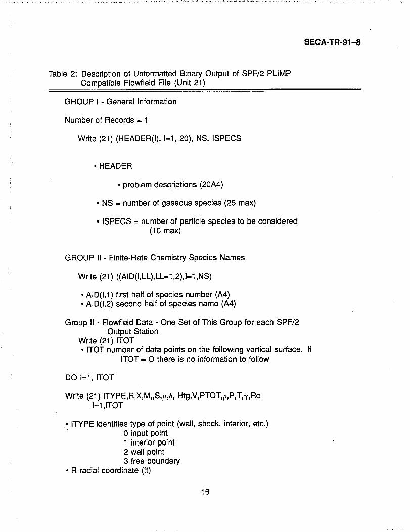
Table 2: Description of Unformatted Binary Output of SPF/2 PLIMPCompatible Flowfield File (Unit 21)
GROUP I-General Information
Number of Records = 1
Write (21) (HEADER(I), I=1, 20), NS, ISPECS
•HEADER
• problem descriptions (20A4)
• NS = number of gaseous species (25 max)
• ISPECS = number of particle species to be considered(10 max)
GROUP II - Finite-Rate Chemistry Species Names
Write (21) ((AID(I,LL),LL=I,2),I=I ,NS)
• AID(I,1) first half of species number (A4)• AID(I,2) second half of species name (A4)
Group II - Flowfield Data - One Set of This Group for each SPF/2Output Station
Write (21) ITOT• ITOT number of data points on the following vertical surface. If
ITOT = O there is no information to follow
DO I=1, ITOT
Write (21) ITYPE,R,X,M,,S,#,6,Htg,V,PTOT,D,P,T,-,/,RcI=1,ITOT
• ITYPE identifies type of point (wall, shock, interior, etc.)0 input point1 interior point2 wall point3 free boundary
• R radial coordinate (ft)
16

SECA-TR-91-8
Table 2: (Continued) Description of Unformatted Binary Output ofSPF/2 PLIMP Compatible Flowfield File (Unit 21)
• X axial coordinate (ft)• M Mach number
0 flow angle (rad)S entropy (ft2/sec2.-°R)
• # Mach angle (rad)• _ shock angle (rad)• Htg gas total enthalpy (ft2/sec 2)• V velocity (ft/sec)• PTOT pitot total pressure (Ibf/ft2)
p gas density (slug/ft3)P pressure (Ibf/ft2)• T temperature (°R)• _,specific heat ratio• Rc gas constant (ft2/sec2-°R)
Write (21) (SPECN,I=I,NS)
• NS number of gas species• SPEN species mole fractions
*Write (21) ((U,V,T,H,p), J=I,ISP)
• ISP number of particle sizes at this point• U axial velocity component (ft/sec)• V radial velocity component (ft/sec)• T temperature (°R)• H enthalpy (ft2/sec2)• p particle density (slug/ft3)
END DO LOOP
*This record is written only for two-phase flowfields.
NOTE: The flowfield data are repetitivelystored on tape as indicatedabove normal surface after normal surface. When ILAST = 0 the end ofthe data has been reached.
flowfield file, the PLIMP code had to be modified to be able to handle the thermodynamicproperties and state variables in the same manner that the SPF/2 code uses them.Previous versions of the PLIMP program had the option of treating ideal gas plumesor plumes that were generated utilizing tables of one dimensionally expanded exhaustproperties generated by the NASA Lewis Equilibrium Combustion Code (CEC)[25].
17

SECA-TR-91-8
These tables allowed the RAMP2 or MOC flowfield to pass along only the independentvariables (entropy, enthalpy and velocity).
Thus, any time the dependent variables (pressure, temperature, Mach number,species, etc.) were needed, the thermodynamic data tables and the independentvariables could be used to determine them. The SPF/2 code however does not utilize atable lookup for the stated variables. The SPF/2 code has four chemistry options; idealgas, frozen, equilibrium and finite-rate. Only the frozen or finite-rate options of SPF/2are considered for inclusion into the PLIMP methodology since all previous as well asall anticipated future plumes will be calculated utilizing this option.
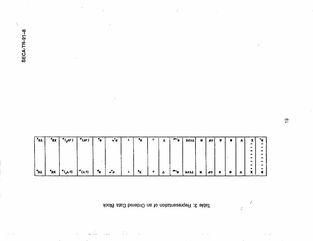
As was previously mentioned, the original version of PLIMP which was structuredfor the MOC and RAMP2 flowfields uses the independent variables (O/F(ET), V, and5') along with the thermodynamic data tables to determine the local flow properties andspecies at any given point in the plume. The SPF/2 code which uses the finite rate orfrozen option calculates all the state properties and species mole fractions in a differentmanner so that much more information must be passed on to the PLIMP code in orderto be able to do impingement calculations. The original PLIMP code only saved thefirst nine variables in Table 3, while the new version of the code has modifications thatcontain all the other variables that are shown in Table 3. In addition to the two ordereddata files of the standard PLIMP code it was also necessary to add another file whichcontains the species mole fractions at each point in the flowfield. As each point is readin from the flowfield file during the ordering of the flowfield, the species mole fractionsare sequentially written to Unit 4 and an index is added to the point. Thus, when thePLIMP code determines the local flow properties at any arbitrary point in the plume, thespecie data can also be determined. Previously, the specie information was determinedfrom the thermodynamic data on the format of the flowfield file, but now PLIMP can alsodetermine species from flowfields which calculate species using other methodologies.One fallout of this modification is that PLIMP will be able to use a RAMP2 finite rateflowfield which it could not previously do.
The original PLIMP code could perform particle impingement force and heating ratecalculations for two phase RAMP2 plumes. However, separate executions of the PLIMPcode were required to do both gaseous and particulate calculations. A fallout of themodifications described in Ref. [21] is the ability to do both the gas and particulate cal-culations during a single PLIMP execution. This greatly reducesthe amount of computertime and post processing of the data which was previously required when two execu-tions were necessary. The last five variables shown in Table 3 are the particle propertyinformation necessary to calculate the force and heating rates to a body due to partic-ulate impingement. The PLIMP particle impingement model is a simplified method forcalculating particle effects to the surface. This simplified approach uses a user inputaccommodation coefficient to determine how much of the particle momentum and en-ergy are actually transferred to the surface. The accommodation coefficient which hasbeen determined experimentally accounts for the interaction of the particles in the shocklayer and at the surface. The accommodation coefficient can vary over a significant range
18
sr-'
O)
!-|
,<OuJ03
O)st--
d_r.T.1 'cl;E_ '(zACl) "(A_) ] de ,_'d A. _ 0 4, mJe 3d/_J, 14 .IO g • A XI u'dJ - -
!i
J:d_i& d_r_ d(_ 01 d(Ad) de veal JL I_ O ,1, I_Je L S/d/Llr" N 40 ,I g L: e A X
s
_1oo1_3_I_G paJepJo u_ jo uo!l_luaseJdaE! :8 elqeJ.

SECA-TR-91-8
depending on the aluminum oxide loading (mass flux) and the shock layer ahead of thebody. For calculations using the PLIMP version of the code a value of .5 is suggested.The existing version calculates the momentum transfer to the surface using Eq. 1 andheating rates using Eq. 2.
np
= pv? (1)i=1
, (_v = a (TE + KE) (2)
where
np
TE = Cvv _ piVi(Ti - T,,,au) (3)i=1
np
gz = _ 0.5 piVi 3 (4)i=1
All heating rate, pressure and contamination options which exist in the PLIMP codefor a RAMP or MOC flowfield are operational for a SPF/2 flowfield.
4.2 Application of the SPF/2/PLIMP Calculation for the TomahawkLC39 Simulations
The set of data for whichthe SPF/2/PLIMP model was validated againstwas im-pingementpressuredatatakenduringa test [26] thatsupportedthe designof the SpaceShuttleLaunchComplex30. Thistest utilizeda 20% AI TomahawkSolidMotor[exitdi-ameter- 8.5 inches,chamberpressure-- 1000 (psia)]anda simulatedMobileLauncherPlatformto determinethe impingementpressuredistributionat 12.2 and 17 ft fromtheTomahawkexitplane (fullscaleshuttleof 214 and 298 ft). Twosets of calculationswereperformed usingthe SPF/2/PLIMP model.
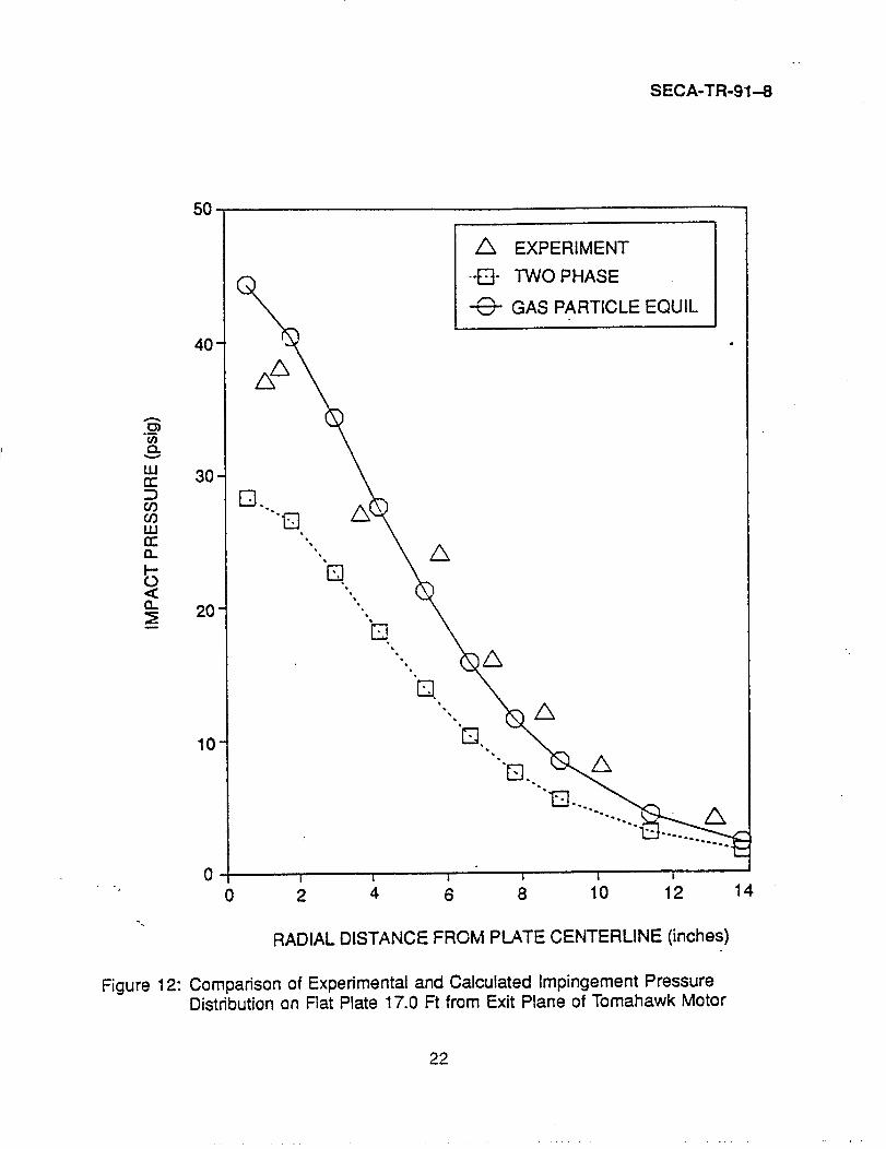
The firstset of calculationswere performedusinga two-phaseSP/F/2 plume. TheSPF/2 plumesolutionwas startedwith a fullycoupled exit plane startlinedeterminedfromthe RAMP2 solutionof the Tomahawknozzle. The resultsof the two-phaseSPF/2and plume impingementcalculationsof impact pressurefor this case are presentedinFigures11 and 12. Figure11 showsa comparisonof measuredand predictedimpactpressuresat 12.2 ft from the exit and Fig. 12 shows the resultsat 17 ft. The two-phase results underpredict the data at both locations. These results are similar to thoseobserved in the pitot pressure correlations shown by Piesik [7].
The second set of SPF/2/PLIMP calculations was made using a SPF/2 plume whichused the gas/particle equilibrium assumption. For this case the particulates are treatedas a gas so that they stay in thermal and dynamic equilibrium with the gas. This is thesame methodologythat was used to develop the Space Shuttle Launch Complex plume
2O

SECA-TR-91--8
I00
/_ EXPERIMENT
•"El" TWO PHASE
GAS PARTICLE EQUIL
80-
Figure 11" Comparison of Experimental and Calculated Impingement PressureDistribution on Flat Plate 12.2 Ft from Exit Plane of Tomahawk Motor
21
°,
SECA-TR-91-8
5O
/X EXPERIMENT
•"E3" TWO PHASE
GAS PARTICLE EQUIL
40-
zxzxffl
m 30
D B.
LLi
0 ,0. "_; 20_
o.
10- "FTJ,
"'F_ A
X
0 l | i t | |
"" 0 2 4 6 8 10 12 14
RADIAL DISTANCE FROM PLATE CENTERLINE (inches)
Figure 12: Comparison of Experimental and Calculated Impingement PressureDistribution on Flat Plate 17.0 Ft from Exit Plane of Tomahawk Motor
22

I
SECA-TR-91-8
induced environments described in Ref. [18]. This methodologyincluding a heat transferanalysis will be further discussed in Section 4.4. The same exit plane startline was usedto start the SPF/2 calculation except that the particulates were put back into the gasphase. Two-phase losses which occurred in the nozzle are included in the startline,but no further two-phase losses occur in the plume. Figures 11 and 12 also show thegas/particle equilibrium results. These impact pressure results compare very well withthe data. One of the conclusions reached in specifying the environments [14,18] wasthat gas/particle equilibrium provided the best correlation with impingement pressuresin the viscous portion of the plume. The SPF/2/PLIMP results assuming gas/particleequilibrium are consistent with previous findings. However, fully coupled two-phasecalculations should be able to exactly predict the correct impingement pressures for two-phase impingement. It is possible that uncoupling the inviscid and viscous plumes forsolid motors cannot adequately describe the flowfield and a fully coupled Navier-Stokesanalysis such as a Level III calculation is necessary.
4.3 Sample Problem Using SPF/2/PLIMP Level II Analysis
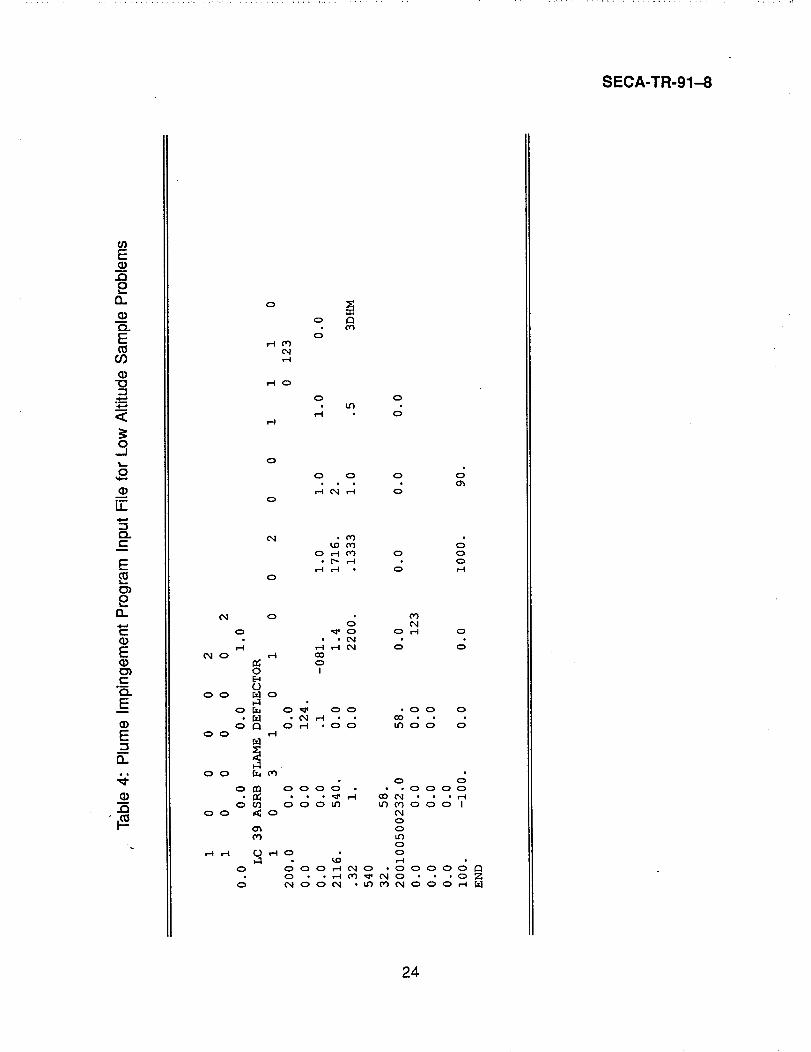
A samplecase for two-phase, low altitude,plume impingementis presentedin thissection. The sample case consists of a Space Shuttle Advanced Solid Rocket Motor(ASRM) plume impinging on the flame deflector. The deflector is a 32 ft long by 58 ftwide flat plate inclined 34 deg to the center of the ASRM plume, which has the nozzle200 ft above the center of the deflector. An accommodation coefficient of .5 was usedfor the analysis. The input file is shown in Table 4. For demonstration purposes only, asingle strip is calculated along the centerline of the deflector, using 5 points along thelength of the deflector. For real calculations more strips and points should be used (say40 points along 40 strips). Table 5 is a printed output of the results.
4.4 Description of a Low Altitude Plume/Thermal Response Model
This section describes a Level II type analysis that was performed to support thelaunch stand design for the Space Shuttle. There were three key areas that wereaddressed in order to develop an overall impingement model for the launch standenvironments: (1) flowfield modeling, (2) model of the particle/gas interaction in theshock layer, and (3) a thermal response model of the structure. This model used anothermixing code [9] along with RAMP and PLIMP, however the conclusions reached duringthe shuttle environment definition can be applied to a RAMP2/SPF/2/PLIMPanalysis forfuture studies. References to RAMP/LAMP can be replaced with RAMP2/SPF/2. It issuggested that the hybrid mixing model (IVIS = -4) be used for low altitude plumes sinceplumes generated with RAMP2/SPF/2 using this model have similar characteristics asthose calculated with RAMP/LAMP.
4.4.1 Plume Flowfield
The nozzle and inviscid plume flowfields were calculated using the RAMPprogram [15]. RAMP is a supersonic equilibrium chemistry two-phase flow code which
23
SECA-TR-91-8
E
2o
O O
O
OO o o o
_ o
_ o
2
_ • ::_ • J
°_ _
_ d_.dd _dd d
-- o_ dddN _mddd_oo _o
_ m
24

Table 5: Plume Impingement Program Output File for Low Altitude Sample ProblemsJ
CASE NO. 1 PAGE 4
ROCKET EXHAUST PLUME IMPINGEMENT ANALYSIS USING THE LOCKHEED/HUNTSVILLE PLUME IMPINGEMENT COMPUTER PROGRAM
LC 39 ASRB FLAME DEFLECTOR
SUBSHAPE IY IZ SHAPE X (SUBSHAPE) Y (SUBSHAPE) Z (SUBSHAPE) PLUME X PLUME R MACH NO-PLUME
IN PLUME SHADED REGIME P IMPACT IMPACT ANGLE PRESS. FORCE MASS FLUX-PLM P-STAT-PLM ....
RAD. CIRV. Q LAMINAR Q-TURBULENT REV. NO. (FT) O TRANSIT O FREE MOLEC SHEAR STRESS M-LOCAL
PARTICLE INFO Q-PARTICLE P IMPACT(PAR) IMPACT ANG(PAR) PRESS FORCE(P) MASS FLUX-PLM KINETIC-PAR THERMAL-PART
1 1 1 PLAT 0.00000E+00 -0.12800E+02 0.00000E+00 0.18939E+03 0.71577E+01 0.13846E+01
YES NO CONT 0.28306E+02 0.34512E+02 0.15131E+07 0.34479E+02 0.14617E+02 0.00000E+00
0.00000E+00 0.23623E+00 0.22036E+03 0.22000E+07 0.00000E+00 0.00000E+00 0.91334E-02 0.92621E+00
0.44643E+04 0.51763E+01 0.35982E+02 0.27669E+06 0.86194E+01 0.38626E+04 0.I1335E+05
1 2 1 PLAT 0.00000E+00 -0.64000E+01 0.00000E+00 0.19469E+03 0.35768E+01 0.18050E+01
YES NO CONT 0.37732E+02 0.34264E+02 0.20179E+07 0.42510E+02 0.14562E+02 0.00000E+00
0.00000E+00 0.24843E+02 0.33754E+03 0.84657E+07 0.00000E+00 0.00000E+00 0.99245E-02 0.11863E+01
0.86651E+04 0.11678E+02 0.34668E+02 0.62421E+06 0.14640E+02 0.12346E+05 0.18121E+05
[k) 1 3 1 PLAT 0.00000E+00 -0.95367E-06 0.00000E+00 0.20000E+03 0.53329E-06 0.19428E+0103 YES NO CONT 0.41251E+02 0.34000E+02 0.22050E+07 0.43656E+02 0.14560E+02 0.00000E+00
0.00000E+00 0.23445E+02 0.36550E+03 0.16792E+08 0.00000E+00 0.00000E+00 0.88809E-02 0.12796E+01
0.10788E+05 0.14778E+02 0.34000E+02 0.78993E+06 0.16679E+02 0.17954E+05 0.20632E+05
1 4 1 PLAT 0.00000E+00 0.64000E+01 0.00000E+00 0.20531E+03 0.35788E+01 0.17442E+01
YES NO CONT 0.35769E+02 0.23702E+02 0.19119E+07 0.41295E+02 0.14605E+02 0.00000E+00
0.00000E+00 0.12869E+02 0.24558E+03 0.26038E+08 0.00000E+00 0.00000E+00 0.51613E-02 0.11625E+01
0.73032E+04 0.96890E+01 0.32922E+02 0.51791E+06 0.13199E+02 0.10325E+05 0.16550E+05
1 5 1 PLAT 0.00000E+00 0.12800E+02 0.00000E+00 0.21061E+03 0.71577E+01 0.13318E+01
YES NO CONT 0.26757E+02 0.33424E+02 0.14302E+07 0.33368E+02 0.14656E+02 0.00000E+00
0.00000E+00 0.60972E+01 0.12638E+03 0.32626E+08 0.00000E+00 0.00000E+00 0.24960E-02 0.97644E+00
0.34673E+04 0.39277E+01 0.31463E+02 0.20995E+06 0.76923E+01 0.31584E+04 0.10128E+05
m0I--I|

SECA-TR-91-8
treats the energy and momentum exchange between the gas and particles. Since theregions of interest on the Space Shuttle launch complex are dominated by the impinge-ment of the viscous portions of the exhaust plumes, it was necessary to perform a plumemixing calculation and superimpose these results on the inviscid RAMP results.
The model chosen to perform the mixing calculation was the LAMP code [9] whichis similar to the LAPP code [16]. The LAMP code is a forward marching finite differencecode which solves the boundary layer form of the governing equations. Necessaryinput to the code is a set of initial jet and free-stream conditions (pressure, temperature,velocity, Prandtl number, Lewis number, and species distributions) as well as an eddyviscosity or Turbulent Kinetic Energy (TKE) model to relate the turbulent shear stress toa viscosity. The selection of an appropriate set of initial conditions as well as the use ofa proper eddy viscosity or TKE model has been the subject of an enormous amount ofstudy by numerous investigators over the past several years.
The initial conditions used for the mixing calculations were obtained by averagingthe exit plane gas properties as calculated by RAMP and expanding or compressingthem to atmospheric conditions using the method of Sukanek [27]. A jet radius was thencalculated so as to get the same mass flow as the rocket motor. It should be noted thatall gas species except aluminum containing species are used to generate the startline.The mass flow rate used to determine the jet size is the total flow rate of the motorincluding the AI203.
The turbulent shear stress model used for these calculations was the 2-equation TKEmodel of Launder et al. [17]. This model was chosen based on previous work presentedin Ref. [13] which used this TKE model to compare with model engine data similar inMach number and density ratio to the SRM sea level plume. One of the drawbacks of aTKE model is the necessityto specify initial distributions of kinetic energy and dissipationrate. The initial kinetic energy is a function of the turbulent velocity fluctuations, and thedissipation rate is related to the kinetic energy via a turbulent length scale. To obtainthe results of Ref. [13], a parametric study was performed using the TKE model, theLAMP code, and a data base of model rocket plume pitot pressure data to determine ageneral set of initial length scales and turbulent fluctuations. This study recommendeda 5 percent velocity fluctuation at the jet edge, a 0.5 percent fluctuation in the remainderof the core and a 0.1 percent velocity fluctuation in the ambient air. The initial turbulentscale length was 2.5 percent of the nozzle exit radius.
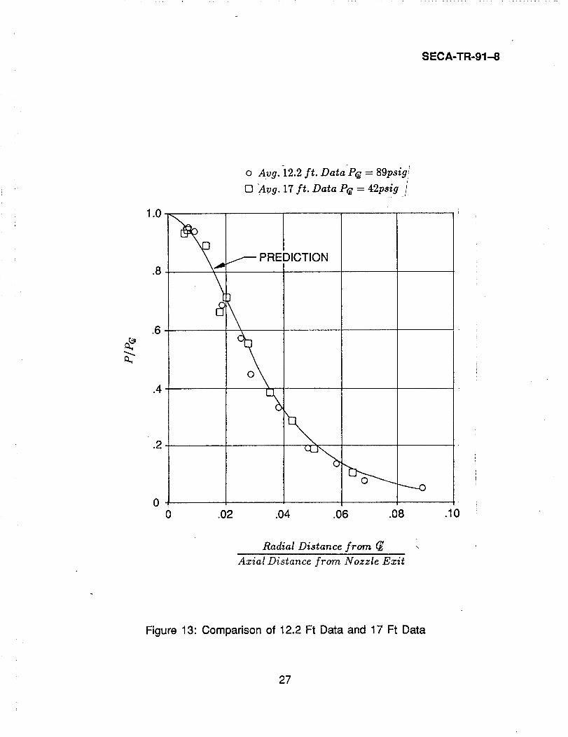
An application [22] of the plume analysis technique is shown in Fig. 13. The dataconsist of an impingement pressuredistribution which results from an 8.5 in. exit diametersolid motor impinging on a flat plate 12.2 and 17 ft from the exit. As can be seen, thecomparison is quite good.
For these calculations, the particles were assumed to be in thermal and dynamicequilibrium with the viscous plume. This assumption is probably adequate, leaving thequestion as to how the particle cloud disperses in the viscous plume. Calculations weremade in which particulate mass was first eliminated from the viscous calculations, thenthe particulate momentum flux was calculated at a particular station of interest, whilemaking the assumptions of either no dispersion or complete dispersion. The results of
26
SECA-TR-91-8
o Avg. 12.2 ft. Data P_ = 89psig/[] 'Avg. 17 ft. Data P_ = 42psig /
1.0
PREDICTION
.8 'k_ i
.6
o
.4.2
00 .02 .04 .06 .08 .10
Radial Distance from _
Axial Distance from Nozzle Exit
Figure 13: Comparison of 12.2 Ft Data and 17 Ft Data
27

SECA-TR-91-8
these calculations did not result in as good an overall prediction as did the previouslymentioned technique. Inherent in this plume model is the assumption that the particlestransfer most of their momentum to the gas before they impinge on the body of interest.For large bodies relative to the plume (MLP deck), the experimental results of Ref. [26]support this assumption. For small bodies relative to the plume, this assumption isprobably not as valid, but the resulting forces on the body are probably close to theresults which are predicted using the plume model presented here.
The results presented here are for the fully viscous plumes since the area of interestin the SRM plume was downstream of the point where the shear layer penetrated to thecenterline. Therefore, the flow properties of the SRM plume which are shown in Figs.14through 18 present only the viscous flow characteristics. A description of the inviscidplume can be found in Ref. [28].
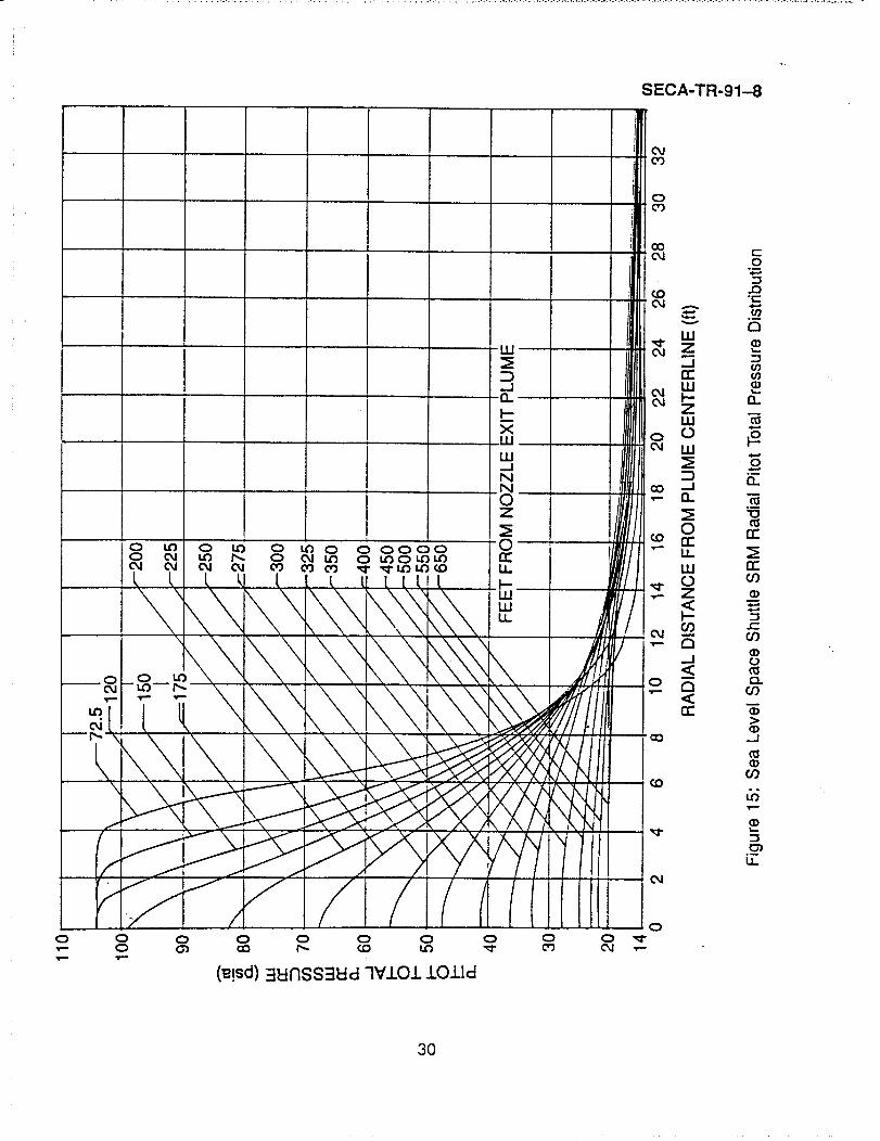
Figure 14 presents the radial distribution of Mach number at various axial stations inthe plume. Figure 15 gives radial distribution of pitot total pressure. Figure 16 shows theradial distributions of the gas recovery temperature. Figures 17 and 18 show the particleproperties of the plume. Figure 17 shows the radial distributions of particle mass fluxwhile Fig. 18 gives the radial distribution of particle total energy (kinetic + thermal) flux.
A limited amount of experimental [26,29] heat transfer data was available whichcould be used to determine an accommodation coefficient which could be used forthermal environment predictions for the MLP. Plumes were developed for the "13tanand Tomahawk motors for which the data was available, but no single accommodationcoefficient could be determined which would correlatethe experimental data, even thoughthe particulatemass fluxes at the regions of interest in the two plumes were approximatelythe same. These results led to investigations of possible impingement flowfield or shocklayer effects which might supply an adequate correlation.
4.4.2 Impingement FlowfieldThe standardmethodof calculatingparticleimpingementheatingto a bodyimmersed
in a two-phaseplume is to consider that the particles pass through the shock layerexperiencingno change in the kineticor thermalenergies. The differencein observedheatingrate and incidentparticle total energy is then accountedfor by means of anaccommodationcoefficient. This method is probablyadequate for very small bodiesrelativeto the plumediameterand at highaltitudeswherethe shockis relativelyclosetothe impingedsurface.At lowaltitudes(lowMach number)andcases wherelargebodiesare impingedby small plumesthe shockahead of the bodymay stand off the bodyatsignificantdistances. In thiscase, as the particlestravel throughthe shock layer theycan be influencedby the relativelydense gas. As a result,the particlescan be turnedas well as heatedand decelerated.
To moreadequatelydeterminethe massand energyfluxesof the particlesthat canactuallystrikea body (suchas the MLP deck) in the SRM plume, particlestreamlineswere traced throughthe shock layer ahead of an impingedbody. A parametricanaly-sis of the particletrajectoriesbehindthe shockwere performedfor the plumesthrough
28

SECA-TR-91--83.0
FROM NOZZLE EXIT (ft)1
72.512o
/_15o ....2.5 _,.,._ _ 175
,7_.300
co. il_ _325I" 1t1.5 ----- 350
°z I3:: / _ 4000 t =
_ _1450,, 500
_!_ "5501.0 - "/--'-651.
, 00 10 20 30 40 50 60 70 80
RADIAL DISTANCE FROM PLUME CENTERLINE (ft)Figure 14: Space Shuttle SRM Radial Distributions of Mach Number
29
SECA-TR-91--8
03
OCO
30

SECA-TR-91.-.8
FROM NOZZLE EXIT (ft)200
225
6000 i I_..5,120I
300
I325
!
5000 ,50I
II
E iO,...4000 ! FROMNOZZLEEXIT (ft)uJ /_ 72.5rr" L=
P- I
=< //_ 15ouJ " ,---- 175= 2(}0"' /// ,,----225I-- 11
" O>UJ>"¢ 3000 Iii' t i 1_//_/7,__1__1/'_"' ; !'/'--/_ 275300250
: ' 325
i 400450I 500
,ooo0 10 20 30 40 50 60 70 80
RADIALDISTANCE FROM PLUMECENTERLINE(ft)
Figure 16: Space ShuttleSRM RadialGasRecoveryTemperatureDistributions
31

SECA-TR-91--8
1oo_:8"7"6-5-4-
3-
2-
FEET FROM NOZZLE EXIT
10 \ T_72.5
/_ 120/J f 150
_C'_ ,'//_/-- 200///--- 250
< /j/-- 3oo350
'x_Ju_
<
o_F-
<a. 0.1 \ ,<
UJW
I1 .'
•. _ \00 10 20 30 40 50 60 70
RADIAL DISTANCE FROM PLUME CENTERLINE (ft)
Figure 17: Space Shuttle SRM Radial Distributions of Undisturbed Plume ParticleMass Flux
32

r_ _ oooooooo_oooI.-- wi _0 kO 0 LO 0 LO kO _ 04 kO 0 "_
. WEZ_
z "7_.
o_ _:_111•
mu_. w,-
121 _
8_rill I I I I ....... 0 _
0 0 0 0 o0 0 o _0 0 _
o ",--
.__(_'/_//nTu) ,00_'AOW3N3 7ViOl qqOliUVa _V3WiS33W4 ,,

SECA-TR-91-8
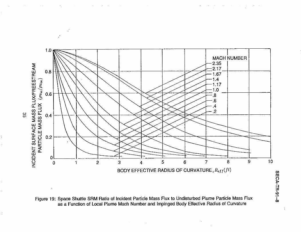
variations in Mach number and effective body radius of curvature. Effective radius ofcurvature is the radius of curvature of a sphere that has the same velocity distributionas the body of interest. The shock standoff distance and velocity distribution behind theshock were determined using the method of Truitt [30]. Once the shock layer propertieswere established, particles of the same size as the SRM plume were tracked throughto the wall and the actual mass and energy fluxes at the surface were calculated. Theresults of these calculations are presented in Figs. 19 and 20. Figure 19 presents theratio of the particle mass flux at the surface to the upstream mass flux (Fig. 17) as afunction of local plume Mach number and body effective radius of curvature. Figure 20presents the ratio of particle total energy at the impinged surface to the free-stream totalenergy (Fig. 18) as a function of local plume Mach number and body radius of curvature.The effective radius of curvature of an infinite flat plate (MLP deck) located at variousdistances from the SRM exit plane are given in Fig. 21. For other arbitrary geometriesthe method presented in Ref. [31] can be used. If the body uses a sphere or a cylinderthen the actual radius of curvature may be used.
4.4.3 Convective Heating RatesThe gaseous convective heating rates are contributors to the overall thermal envi-
ronment produced by solid rocket exhaust plume impingement. Since the SRM plumeimpingement problem of interest involves predominantly stagnation type heating, a sim-plified approach to calculating the convective heating environment was adopted for theoverall model.
Stagnation point heating rates for a 1 ft sphere were calculated at various pointsdown the centerline of the SRM plume. These calculations were made using the methodof Marvin and Diewert [32] and the computer code of Ref. [33]. Additionally,the viscousplume is highly turbulent. Previous investigators [34] have shown that turbulence in theexhaust plume amplifies the heating rate one would normally predict. Reference [34] hasa correlation of amplificationfactor as a function of local Eckert number and mean velocityfluctuation. Amplification factors were calculated for the SRM plume and applied to thestagnation point heating rates previously calculated. The resultant centerline distributionof stagnation point heating rates for the SRM plume are shown in Fig. 22.
The primary application of the SRM plume was to predict the thermal environmentto the MLP deck (a large body relative to the plume). To account for variations in totalpressure and temperature of the centerline of the plume, Fig. 23 was generated. Thisfigure presents Iocal/centerline heating rate ratios at various axial stations in the SRMplume. The use of Figs. 22 and 23 allows the designer to determine a convective heatingrate at any point in the plume, assuming that the plume is impinging on an infinite flatplate.
It is possible to use the data presented in Figs. 22 and 23 for small bodies whichare impinged on by the SRM plume. To obtain a Iocal/centerline heating rate-ratio fora small body use the following equation:
34
s
MACH _IUMBER
_ 0.8- - '
<_ 0.4
0,O 0 1 2 3 4 5 6 7 8 9 10Z
BODY EFFECTIVE RADIUSOF CURVATURE, Reii(ft) (I)mo
-t
Figure 19: Space Shuttle SRM Ratio of Incident Particle Mass Flux to Undisturbed Plume Particle Mass Flux (_as a Function of Local Plume Mach Number and ImpingedBody Effective Radius of Curvature

eJnleAJnOjo sn!peEI eA!lOeJl::l,_PO8peSu!duJl pueJequJnN qOelhieuJnld leoo-I 1o uo!loun:l e se xnl:l/_6JeU3 lelOl elo!lJed
"_- ewnld peqmls!pun ol xni-I/(SJeu:l lelOl elo!lJed ]uep!oul jo o!leE! _EI8 elllnLISeoeds :0_ ejnl3!-!o}I
r¢t--
I
0uJ
(t/)//_E ' =IElnXVAElno 30 SNIOVEi 3AIZO3-1:I3 AEI08
01. 6 8 L 9 S _ I_ _ I. 0
_ m_mm
•o "n
XIO to
g.__ O-er_>17"- m_
mOZl.'l. - z_
_r--
L9"L - ._. 8"00mLL'_ - "<z.---.Ill
0EI381AInNHOVIAI "_ _<I O'L 8
i

",- _EIS ell;nqs coeds eqi Aq uodn po6uldwl, e_elcl lel-I OllUUUl.. ue Jo eJnlet_no jo sn!peE! eA!lOolE! "L;_oJn61-1.O_|
13C:
!
< (11)3NVqd 11X3 37ZZON I/_OEI-I3ONVISIO 7VIXVoI11
OOZ 009 OOC-; 00_' 00_ 00_ O0I. 0
I I 1 o m131EIOHIEIONXVIAiEIAS1109370H1SFIVHXq30 3E)03 -11
mo
/ _ -4
&t1131NO=J9c
7VOO73SI70_ oo r..O co
/ >103(3 cl71N 71oc
<>
£_ -4c33m
0g ½
SECA-TR-91--8
38

SECA-TR-91-8
DISTANCE FROM NOZZLE EXIT (ft)
250 I
300350
,oon,- 500r,,9z 550
650
< \\\ i
w 0.6 72.5
wT" k_ 150z 120
200u.II--z 0.4
0.2 \ / _\
o0 10 20 30 40 50
RADIAL DISTANCE FROM PLUME CENTERLINE (ft)
?
Figure 23: Space Shuttle SRM Local-to-Centerline Convective Heating Rate Ratio
39
SECA-TR-91-8
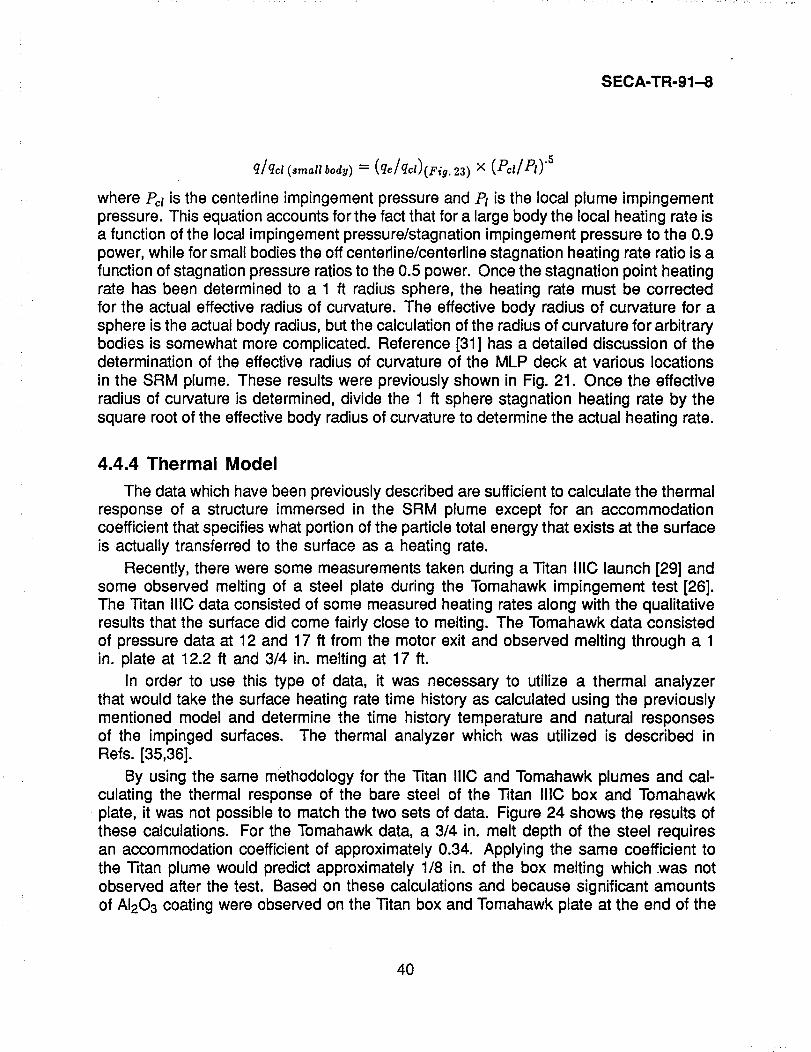
q/qcl (small body) = (qe/qcl)(Fig. 23) × (Pcl/el) "5
where Petis the centerline impingement pressure and Pt is the local plume impingementpressure. This equationaccounts for the fact that for a large body the local heating rate isa function of the local impingementpressure/stagnation impingement pressure to the 0.9power, while for small bodies the off centerline/centerlinestagnation heating rate ratio is afunction of stagnationpressure ratiosto the 0.5 power. Oncethe stagnation point heatingrate has been determined to a 1 ft radius sphere, the heating rate must be correctedfor the actual effective radius of curvature. The effective body radius of curvature for asphere is the actual body radius, but the calculation of the radius of curvature for arbitrarybodies is somewhat more complicated. Reference [31] has a detailed discussion of thedetermination of the effective radius of curvature of the MLP deck at various locationsin the SRM plume. These results were previously shown in Fig. 21. Once the effectiveradius of curvature is determined, divide the 1 ft sphere stagnation heating rate by thesquare root of the effective body radius of curvature to determine the actual heating rate.
4.4.4 Thermal Model
The datawhichhavebeen previouslydescribedare sufficientto calculatethe thermalresponseof a structureimmersedin the SRM plume except for an accommodationcoefficientthatspecifieswhatportionofthe particletotalenergythatexistsatthe surfaceis actuallytransferredto the surface as a heatingrate.
Recently,thereweresomemeasurementstakenduringa Titan IIIC launch[29] andsome observed meltingof a steel plate duringthe Tomahawkimpingementtest [26].The Titan IIIC dataconsistedof somemeasuredheatingratesalongwiththe qualitativeresultsthat the surfacedid come fairlycloseto melting.The Tomahawkdata consistedof pressuredata at 12 and 17 ft fromthe motorexit and observedmeltingthrougha 1in. plate at 12.2 ft and 3/4 in. meltingat 17 ft.
In order to use this type of data, it was necessary to utilize a thermal analyzerthat wouldtake the surface heatingratetime historyas calculatedusingthe previouslymentionedmodeland determinethe time historytemperatureand natural responsesof the impingedsurfaces. The thermal analyzer which was utilized is describedinRefs. [35,36].
By usingthe same methodologyfor the Titan IIIC and Tomahawkplumes and cal-culating the thermal responseof the bare steel of the Titan IIIC box and Tomahawkplate, it was notpossibleto matchthe two sets of data. Figure24 showsthe resultsofthese calculations.For the Tomahawkdata, a 3/4 in. melt depth of the steel requiresan accommodationcoefficientof approximately0.34. Applyingthe same coefficienttothe Titan plumewouldpredictapproximately1/8 in. of the box meltingwhich.was notobservedafter the test. Basedon these calculationsand becausesignificantamountsof AI203 coatingwere observedonthe Titan boxandTomahawkplate at the endof the
4O

J
/1.0 /" .......
/
///// TOMAHAWK NO DEPOSITION MODEL.75
m coJ_o co
/ LU
'_" / Z
-r ,¢"}-- -- TITAN O DEPO IT oa. -7uJ .5 ............ .05 _-
-" ZI--
om V-
0
.25 _ .025 uJ, ,.,3
0 .1 .2 .3 .4 .5 .6 .7 .8 1.0 c_I"!1
ACCOMMODATION COEFFICIENT o|
--III
Figure 24: l]tan Box II and Tomahawk 17-Ft Melt Thickness and Aluminum Oxide Layer Thickness as _oa Function of Particle Surface Accommodation Coefficient

SECA-TR-91-8
firing, it was decided to investigate an AI203 deposition model to see if a coating mightpossibly correlate the two pieces of data and allow a single accommodation coefficientthat would match the data.
The resulting thermal model used the time history of gas recovery temperature, coldwall convective heating rate, particle mass and energy fluxes at the surface and anassumed accommodation coefficient as input conditions. The model starts off with coldsteel and keeps track of how much AI203 is deposited on the surface until enough hasbeen added to build up a 0.002 in. layer at which point a node is added. The mass isadded to the surface via the following:
t+dtP
= (/pA 2o3)/ (pV) dA
t
where A is the incremental AI203 thickness, a is the accommodation coefficient,pAI203
is the specific density of AI203 and (pv)w is the mass flux at the surface. Masscontinues to build up on the surface in 0.002 in. layers until the surface temperatureof the AI203 reaches melt temperature of 4170°R. Heat is added to the surface at thesurface temperature by the following:
QItw = Qc,cw,((ToR - Twau)/(ToR - 540)) + a (pv)w (Hp - Hw)
where QHw is the actual heating rate to the surface at the surface temperature, Qc,cw.is the input cold wall heating rate, ToR is the gas recovery temperature, Tw_,zlis thesurface temperature, Ep is the particle enthalpy at the surface which is determined bydividing the particle total energy at the wall by the particle mass flux at the wall, andHw is the enthalpy of aluminum oxide evaluated at the surface temperature. Once thesurface has heated up to 4170°R, heat continues to be added and the AI203 is allowedto absorb the heat of fusion and then super heat. This process continues until enoughheat has been conducted through the AI203 layer to the first steel node to elevate itstemperature to the melting point. Then the steel node is allowed to absorb its heat offusion. Oncethis occurs the steel node and the entire AI203 deposition layer is removedand the entire deposition process continues until the plume no longer influences thesurface. Many other assumptions, node sizes, etc., were made prior to finalizing thethermal model. The model which was finally chosen did the best job of correlating thelimited amount of data.
When this thermal model was applied to the Titan IIIC and Tomahawk data, an• accommodation coefficient of 0.55 resulted in no melting of the Titan IIIC box sur-
face, and 3/4 in. of steel melted for the Tomahawk case. The results of these cal-culations are presented in Fig. 25. This figure presents the melt thickness and AI203deposition thickness versus accommodation coefficient. The model when applied tothe Titan data predicted no melting at any accommodation coefficient. Figure 26presents a time history of what the model predicts for the response of the Titan box
42

IJ
o0 r#
TOMAHAWKOEPOSmONMo z
" 7 5 I ' //e.-0 / or)e- ILl",_, Z
__ o_n -r"
. _ .5 _" -- .05
co I-;, J /--- TITAN zDEPOSITIONTHICKNESS O
0
__ " .025 LU.25 / c3
/ .f---- -. ToM. wKDEPOSITION THICKNESS¢,1
00 .1 .2 .3 .4 .5 .6 .7 .8 1.0
ACCOMMODATION COEFFICIENT mO!
-4|
t4)
Figure 25: 3]tan Box II and Tomahawk 17-Ft Melt Thickness and Aluminum Oxide Layer Thickness asa Function of Particle Surface Accommodation Coefficient

/---- SURFACE TEMPERATURE
_0oo _f--_<,. I_" 4000 "_-
0 0al::v 0ILl _"rr" ",_.
3000 .03 coco.1_ nr" Z
Illn O
!11
.... (I)tee! 0
13.
1000 ----- " .01 _£3
_ .5" _0 / 0 u)m2.4 3.0 4.0 5.0 6.0 o
TIME (sec) -q|
,...l
Figure 26: Titan IIIC Box 2 Thermal Analysis Results _o

SECA-TR-91-8
to the plume. The AI203 surface temperature superheats to about 5200R while the steelsurface barely reaches melt temperature but cannot absorb the heat of fusion and thusdoes not melt. Also shown on this figure is the deposition thickness time history andthe temperature distribution through the steel surface. The AI203 deposition thicknesswhich is predicted is consistent with the observed layer thickness following the test.
Probably the biggest factor in allowing the correlation of the two pieces of data wasallowing a superheated molten layer of AI203 to form on the surface. Once the surfacelayer has absorbed the heat of fusion of the AI203 and the temperature has risen abovethe melt temperature the heat of fusion of the incoming AI203 energy flux cannot beadded to the surface, which effectively lowers the surface heat load.
Finally, this entire model was applied to a point on the edge of the SRM exhausthole of the MLP. It is expected that this locationshould be subjected to a fairly high heatload and would be indicative of the amount of deck melt that might be expected. Theresults of these calculations are shown in Fig. 27. This figure indicates that the steelsurface reachesthe melt temperature but does not absorb enough heat to melt. There isprobably some slight surface melting. Also shown on this figure is the temperature-timehistory at different depths in the plate.
45

elOHlsneqx=lPills d-IIAI_oe6p:! jo slS,{leuVlewJeql to sllnsel:l :l_ eJn6!-t
I--|
_: (oes) 3_110W
O'L 0"9 0"(3 0"t7 _'g0'0, / 0
°m SS=iN>IOIH/NOIIISOd3CI 'tO73
o /1__'f01.0" 0001.
z_ _-7 ,___m 090" 000g
5" "_t0
0
OgO........ O00g -4
3WAIVWI ldV_3130V=IUFI87 >00017C
m
30V.._lUn___ "-"
0
000(3
3wnlvwqa_31
0009,f

SECA-TR-91-8
Section 5LEVEL II! LOW ALTITUDE IMPINGEMENT ANALYSIS
The highestlevel of sophisticationfor low altitude impingementmodelingwouldentailutilizingthe more recentlydevelopedNavier-Stokescodes. These codes havethe potentialfor modelingthe entireexhaustplume includingthe structurethat is beingimpinged.Thesecodeshavebeen extendedto threedimensionsso that multipleplumescan theoreticallybetreatedalthoughconsiderablevalidationexerciseswouldbe required.It shouldbe notedthat Level III CFD analysisare computationallyfairly expensiveandcan require significantamounts of labor to set up the geometry and properly initializethem. CFD models would probably only be used if a Level I or II analysis could notadequately address particular problems.
An example os a Level III model is the FDNS code [10]. FDNS is a implicit Navier-Stokes solver which has several turbulence model options. It also has ideal, frozen,equilibrium and finite-rate chemistry options. Presently, under NASA funding, the codeis being upgraded to treat two-phase flows. A Lagrangian particle treatment has beenadded and preliminary check cases have been completed. Figure 28 presents thedistribution of impact pressure for the experimental data previously shown in Fig. 11.This particular case was modeled with the flat plate as a part of the solution. Thecalculations are within 7 percent of the measured results. These calculations includedtwo-phase flow (22% AI), finite-rate chemistry and a two-equation turbulence model. Theturbulence model is the standard model which is used by FDNS to calculate plumes andwas not adjusted for this case. The solution was initiated in the combustion chamber.This is an example of the type of results that can be expected from a Navier-Stokessolver. However, these codes must be exercised against a large amount of experimentaldata and configurations before they can be regularly used for low altitude impingementpredictions.
47

SECA-TR-91-8
120
100 _ && z_ Experience with FONDUE-FYREPRESENT PREDICTION
8O
-_. 60o..
40 - z_ z_
2O
0 1 !0 5.O 10 15
R (inches)
Figure 28: Tomahawk Impingement on Plate 12.2 Ft from Nozzle Exit (Five Particle SizesTwo-Phase Flow Calculation)
48

SECA-TR-91-8
Section 6REFERENCES
[1] Smith, S.D., "High Altitude Supersonic Flow of Chemically Reacting Gas-ParticleMixtures - Volume III - RAMP2 - Computer Code User's and Applications Manual,"Lockheed Missiles & Space Company, Huntsville, AL, LMSC-HREC TR D867400-III, Oct. 1984.
[2] Smith, S.D., "User's Manual - Variable O/F Ratio Method of CharacteristicsProgramfor Nozzles and Plume Analysis," LMSC-HREC D162220-1V,Lockheed Missiles &Space Co., Huntsville, AL, June 1971.
[3] Doo, Y.C. and Nelson, D.A., "Direct Monte Carlo Simulation of Small BiopropellantPlumes," AFRPL TR-86-100, Aerospace Corp., Los Angeles, CA, Jan. 1987.
[4] Chirivella, J.E., "Direct Simulation Monte Carlo of Vacuum Plumes - AFE RCSPlumes," ER-SP-1016, Engo Tech Systems, Inc., Tujunga, CA, Sep. 1988.
[5] Heuser, J.E., Melfi, UT., Bird, G.A., and Brock, F.J., "Analysis of Large SolidPropellant Rocket Engine Exhaust Plumes Using the Direct Simulation Monte CarloMethod," AIAA-4-0496, paper presented at the AIAA 22nd Aerospace SciencesMeeting, Reno, Nevada, Jan. 1984.
[6] Piesik, E.T. and Roberts, D.J., "A Method to Define Low-Altitude Rocket ExhaustCharacteristics and Impingement Effects," J. of Spacecraft and Rockets, 7, April1970, pp. 446-451.
[7] Piesik, E.T., "Aluminized Propellants and a Method Defining Low-Altitude ExhaustPlumes", J. of Spacecraft and Rockets, Vol. 23, No. 2, March-April 1986, pp.215-221.
[8] Dash, S.M., Pergament, H.S., and Thorpe, R.D, "A Modular Approach for the Cou-pling of Viscous and Inviscid Processes in Exhaust Plume Flows", 17thAerospaceSciences Meeting, New Orleans, Jan. 1979.
[9] Ratliff, A.W. et al., "Chemical Laser Analysis Development;Vol. 1, Laser and MixingProgram and User's Guide," Lockheed Missiles & Space Company, Huntsville,AL,Oct. 1973.
[10] Chen, Y.S., "Compressible and Incompressible FlowComputations with a PressureBased Method," AIAA-89-0286, 27th Aerospace Sciences Meeting.
[11] Anon., "Saturn V Launch Complex Plume Induced Pressure and Thermal Environ-ment," The Boeing Co.
[12] Will, C.F., "Thermal Environment Computer Program for Solid Rocket ExhaustAnalysis," TN-AP-69-419, Chrysler Space Division, June 1990.
[13] Smith, S.D., "Revised Predictions of the SRB Plume Impingement Pressures onthe MLP (LC39) During Uft-Off," LMSC-HREC TR D568286, Lockheed Missiles &Space Co., Huntsville, AL, April 1978.
[14] Environment and Test Specification Levels Ground Support Equipment for SpaceShuttle System Launch Complex 39. Vol. 11 of 11, Thermal and Pressure Part 2
49

SECA-TR-91-8
of 2, Specific Temperatures of Selected Parts of LC39 GP 1059 Kennedy SpaceCenter, FL, July 1977.
[15] Penny, M.M., Smith, S.D., et al., "Supersonic Flow of Chemically Reacting Gas-Particle Mixtures," LMSC-HREC TR D496555-11/11,Lockheed Missiles & SpaceCompany, Huntsville, AL, Jan. 1976.
[16] Mikatarian, R.M., et al., "A Fast Computer Program for Non Equilibrium RocketPlume Predictions," AFRPL-TR-72-94 Aerochem Research Labs, Princeton, NJ,Aug. 1972.
[17] Launder, B.E., Morse, A., Rodi, W., and Spalding, D.B., "The Prediction of FreeShear Flows. Presented at Langley Working Conference on Free Turbulent ShearFlows," NASA-Langley Research Center, Hampton, VA, July 1972.
[18] Smith, S.D., "Definition of the Viscous Sea Level Space Shuttle Solid RocketMotor(SRM) Exhaust Plume, Impingement Flowfield and Thermal Properties Necessaryto Perform a Thermal Response Analysis of the LC39 MLP," LMSC-HREC TND697736, Lockheed Missiles & Space Co., Huntsville,AL, Nov. 1979.
[19] Tevepaugh, J.A., Smith, S.D., and Penny, M.M., "Assessment of Analytical Tech-niques for Predicting Solid Propellant Exhaust Plumes," AIAA Paper 77-711, AIAA19th Fluid and Plasmadynamics Conference, Albuquerque, NM, June 1977.
[20] Fay, J.A. and Riddell, F.R. "Theory of Stagnation Point Heat Transfer in Disasso-ciated Air," J. of Aerospace of the Sciences, Vol. 25, No. 2, Feb. 1958, pp. 73-85.
[21] Smith, S.D., et al., "Model Development for ExhaustPlume Effects on LaunchStandDesign," SECA-89-20, SECA, Inc., Huntsville, AL, Sep. 1989.
[22] Ludwig, C.B., et al., "Standardized Infrared Radiation Model (SIRRM)", Volume I,APRPL-TR-54, Aug. 1981.
[23] Walker, J., et al., "Handbook of the Standardized Infrared Radiation Model(SIRRM)," Volume II, AFRPL-TR-81-61, Aug. 1981.
[24] Dash, S.M., et al., "The JANNAF Standard Plume Flowfield Model (SPF/2), Vol, II- Program Users Manual," SAI/PR TR-16-11, SAIC, Princeton, NJ, May 1984.
[25] Svehla, R.A., and McBride, B.J., "FORTRAN IV Computer Program for Calculationof Thermodynamics and Transport Properties of Complex Chemical Systems,"NASA TN D-7056, Jan. 1976.
[26] Seymour, D.C., Greenwood, T.F., and Smith S.D., "Plume Impingement PressureMeasurements Taken During Sea Level Firings of a Tomahawk Motor," JANNAF11th Plume Technology Meeting, Huntsville, AL, July 1979.
[27] Sukanek, P.C., "Matched Pressure Properties of Low Altitude Plumes," AIAA J.15, No. 12, Dec. 1977.
[28] Smith, S.D., "Space Shuttle Solid Rocket Motor (SRM) Exhaust Plume DefinitionsSea Level to SRB Separation," LMSC-HREC TM D496879, Lockheed Missiles
and Space Company, Huntsville, AL, Aug. 1976.[29] "Test Report for Titan IIIC SRM Plume Impingement Pressure Measurementsat
LC40 - 13 Dec. 1978. KSC-DL-126 Planning Research Corporation, KennedySpace Center, FL, Sep. 1979.
[30] Truitt, R.W., Hypersonic Aerodynamics, The Ronald Press Company, New York,1959.
5O

SECA-TR-91-8
[31] Wojciechowski, C.J. and Rader, R.J., "A Method of Calculating StagnationRegionConvective Heat Transfer to Arbitrary Surfaces Immersed in the Space ShuttleAltitude Control System Plumes," LMSC-HREC D162334, Lockheed Missiles andSpace Company, Huntsville, AL, May 1970.
[32] Marvin, J.C., and Diewert, G.S., "Convective Heat Transfer in Planetary Gases,"NASA TR R-224, July 1965.
[33] Rader, R.J., "Input Guide for the STAG-q Computer Program," TN-241-1152,Northrop Services, Inc., Huntsville, AL, Oct. 1972.
[34] Weeks, Thomas M., "Influence of Free-Stream Turbulence on Hypersonic Stag-nation Zone Heating," AFFDL-TR-67-195, Air Force Flight Dynamic Lab., Wright-Patterson Air Force Base, OH, May 1968.
[35] Pond, J.E., "A Small Thermal Analyzer Package with Simplified Input," LMSC-HREC D162533, Lockheed Missiles and Space Company, Huntsville, AL, Feb.1971.
[36] Environment and Test Specification Levels Ground Support Equipment for SpaceShuttle System Launch Complex 39. Vol 11 of 11, Thermal and Pressure Part 2of 2, Specific Temperatures of Selected Parts of LC39 GP 1059, Kennedy SpaceCenter, FL, July 1977.
[37] Snedeker, R. S. and Donaldson, DuP. C., "Experiments on Free and ImpingingUnderexpanded Jets from a Convergent Nozzle," Advanced Research ProjectsAgency Report 63, DDC AD 461622, Sep. 1964.
[38] Unpublished Flat Plate Rocket Exhaust Impingement Data Obtained for a 20:1Scale F-1 Rocket Engine from Marshall Space Flight Center, Huntsville, AL.
[39] Moore, G. R. and Soo Hoo, G., "Comparison of Static Rocket Motor Plume Predic-tions Using the JANNAF SPF-1 Model with Experimental Plume Measurements,"JANNAF 13th Plume Technology Meeting, Houston, TX, CPIA Publication 357,April 1982, pp. 143-148.
51