NASA Contractor Report 191536

ICASE Report No. 93-69

1100

= ICASE USIMULATIONS OF DIFFUSION-REACTION EQUATIONS WITHIMPLICATIONS TO TURBULENT COMBUSTION MODELING

Sharath S. Girimaji

DTIC'<- DEC 2 2i1' 33,J.I.-

NASA Contract No. NAS 1-19480September 1993

Institute for Computer Applications in Science and EngineeringNASA Langley Research CenterHampton, Virginia 23681-0001

Operated by the Universities Space Research Association

pubu M_4 ..., 93-30651

National Aeronautics andSpace Administration

Langley Research CenterHampton, Virginia 23681-0001 93 12 17049

ICASE Fluid Mechanics

Due to increasing research being conducted at ICASE in the field of fluid mechanics,

future ICASE reports in this area of research will be printed with a green cover. Applied

and numerical mathematics reports will have the familiar blue cover, while computer science

reports will have yellow covers. In all other aspects the reports will remain the same; in

particular, they will continue to be submitted to the appropriate journals or conferences for

formal publication.Accesion For

NTIS CRA&IDTIC TABUnannounced Q

Justification

By...................... ...

Avu~bc.;;[y Co¢ces

[Dist I Avti! a-dicr

DTIC QUAMITY INSECTED 3

SIMULATIONS OF DIFFUSION-REACTIONEQUATIONS WITH IMPLICATIONS TO TURBULENT

COMBUSTION MODELING

Sharath S. Girimaji'

Institute for Computer Applications in Science and Engineering

NASA Langley Research Center

Hampton, VA 23681

ABSTRACT

An enhanced diffusion-reaction reaction system (DRS) is proposed as a statistical model

for the evolution of multiple scalars undergoing mixing and reaction in an isotropic turbulence

field. The DRS model is close enough to the scalar equations in a reacting flow that other

statistical models of turbulent mixing that decouple the velocity field from scalar mixing and

reaction (e.g. mapping closure model, assumed-pdf models) cannot distinguish the model

equations from the original equations. Numerical simulations of DRS are performed for

three scalars evolving from non-premixed initial conditions. A simple one-step reversible

reaction is considered. The data from the simulations are used (i) to study the effect of

chemical conversion on the evolution of scalar statistics, and (ii) to evaluate other models

(mapping-closure model, assumed multivariate P-pdf model).

'This research was supported by the National Aeronautics and Space Administration under NASA Con-tract No. NAS1-19480 while the author was in residence at the Institute for Computer Applications inScience and Engineering (ICASE), NASA Langley Research Center, Hampton, VA 23681.

in.i

1 Introduction

Turbulent combustion is an interplay of several complex physical processes: e.g. turbulent

transport, scalar mixing, chemical reaction, heat release. Turbulent transport is present

only in inhomogeneous flows where the gradients of the scalar statistics are non-zero. Scalar

mixing- which is important in isotropic as well as inhomogeneous flows- comprises two mech-

anisms: the effect of the velocity field, which is to cascade scalar energy to smaller length

scales; and molecular diffusion, which typically acts at smaller scales to reduce scalar fluctua-

tions. Chemical reaction is a local phenomenon which converts scalar species from reactants

to products. In problems of interest in combustion, chemical conversion is accompanied by

heat release and, hence, density reduction. If the heat release is large enough, the resulting

buoyancy forces can modify the velocity field in which the scalars reside. If the heat release

is small, the modification of the velocity field is negligible.

In the scalar-statistics equations, the terms representing several of the above processes

need closure modeling. A turbulent combustion model is really a composite of these closure

models of the individual processes. Often, when calculations from the composite model are

in poor agreement with either experimental or direct numerical simulation (DNS) data, it

is difficult to isolate the underlying cause (the model of a specific physical process) of the

disagreement. For this reason, it is useful to construct sample test problems where only one

or few of the physical processes are important (other processes are either negligible or or

completely absent). Data from the numerical simulations of such a test problem can be used

to construct and validate the individual models.

The divide-and-conquer approach has proved especially successful in the understanding

and modeling of the inert scalar mixing process. Eswaran and Pope (1988), and subsequently

others, performed DNS of inert scalar fields evolving from non-premixed initial conditions in

constant-density, isotropic turbulence. In this first step, the effect of velocity field on scalar

mixing is studied, without the complexities of spatial inhomogeneities or chemical reaction.

One of the chief findings of DNS studies is that (for the range of Reynolds number inves-

tigated, R,\ 30 - 90) the velocity field only affects the timescale of the scalar pdf evolution.

In appropriately normalized time, the scalar pdf evolution is independent of the velocity

field. This insight gained from the DNS studies spawned reasonably successful modeling

approaches in which the scalar evolution is considered only in the normalized time, thus

decoupling the velocity field from the scalar field. The models are: the mapping closure

model (Kraichnan 1989, Girimaji 1992b), the Johnson-Edgeworth translation (JET) models

of Madnia et al (1992) and the assumed /3-pdf model (Girimaji 1991a).

Study of a test case which combines scalar mixing with chemical chemical reaction in

isotropic turbulence should be a useful second step towards the ultimate objective of un-

derstanding and modeling turbulent combustion. In this work, we analyze the test-case

equations and propose a statistical model for the scalar (species and temperature) evolu-

tion. The model equation set is a diffusion-reaction system (DRS). The model accounts for

the effect of the velocity field via a time-dependent diffusion enhancement coefficient factor.

The model equations are close enough to the original turbulent-reaction equations that other

models which decouple the velocity field and scalar-field mixing cannot distinguish between

the two sets of equations. Numerical simulation of the model DRS equations is computation-

ally much less intensive than DNS of the original equations and may.serve nearly as useful a

purpose in understanding and evaluating turbulent combustion models. Simulations of the

DRS equations are performed to (i) shed some light on the effect of reaction on scalar field

evolution, and (ii) evaluate the performance of other models (developed originally for inert

mixing) against reacting scalar data.

The organization of the remainder of the paper is as follows. In Section 2, the relevance

of the (enhanced) DRS to turbulent combustion is investigated in more detail. Numerical

simulations of DRS equations is performed in in section 3. A brief description of the numerics

employed in the simulations is also provided. Section 4 contains the results of the simulation

and a discussion of its implications to turbulent combustion modeling. The paper concludes

in Section 5 with a summary.

2

2 Enhanced diffusion-reaction system as a model ofturbulent reactive flows

Consider the mixing and reaction of n scalars (of mass fractions 0,, a = 1,.. n) in a

velocity field u(X, t) evolving under Navier-Stokes. The following assumptions are made: i)

no body force, ii) no radiative heat transfer, iii) scalar diffusion governed by Fickian law, iv)

low Mach number (hence, pressure is considered nearly a constant), and v) high Reynolds

number (hence, the viscous contribution to the energy equation is negligible). Subject to

the above assumptions, the scalar and temperature (T) evolution equations are

P[.--- + u.-`] --[pD-•-0+ .,, (1)

andahT ahT a - aT n nat-ah + ui = a .[,\]aT-I + 1 a [ph TD. E owo. (2)

at Ox Oi xi Of1 Xi 01 (2)Or1In the above equations, DQ and w0, are respectively the Fickian diffusion coefficient and

the chemical production rate of species a. The heat conductivity of the mixture is A. The

enthaly of formation and thermal enthaly of species a are ho and hiT. The total thermal

enthalpy of the mixture, (hT), is given by

n

hT = T• h'. (3)Of=1

The pressure (p), density of the mixture (p) and the mass fractions are related through the

equation of state which could be the ideal gas law. It is assumed that the temperature and

the chemical source terms can be determined given the thermal enthalpy and mass fractions.

Subject to homogeniety of the turbulent velocity field, the joint pdf of scalar composition

and thermal enthalpy, F(hT, 4), evolves according to (Pope 1985)

p(hat ýFh ) [F(T,D)T- RT}] (4)

-, -

In the above equation the conditional diffusion of temperature (OT) and scalar (00,) are

given bya OT _ 0 (5)

O[AX+ F_ ph-OD],, ,•_),

3

and

S= [-D-, 8 T, ,), '(6)

where, the notation (blr) denotes the conditional mean of b with respect to r. The pdf source

term of temperature (RT) and scalar (R/) due to reaction are given by

1t

RT how., (7)

and

R4. = w-. (8)

While the source terms due to reaction are closed in terms of temperature and scalar compo-

sition, the scalar diffusion terms need closure modeling. The modeling of these terms require

that the effect of the velocity field on the scalar field be known, at least approximately.

2.1 Lagrangian coordinate analysis

The effect of the velocity field on the scalar field is examined in Lagrangian frame of reference

(x, t) which is cartesian. For the sake of this analysis, the velocity field is assumed to be

isotropic. The Eulerian coordinate X is now nonstationary, curvilinear and nonorthogonal,

evolving according toOX(x, t)(90 ,t) = U[X(x,t),tI. (9)

The Eulerian conditional diffusion can now be written in terms of the Lagrangian deriva-

tives:

O ( [ D0 -[D.T 0a .]IT, )). (10)oX-o a Xi ak--J OM, a•, Xo. a,, -

DefineaxiC.,(x) = •// (11)

The correlation between CG. and the scalar derivatives in the Lagrangian coordinates is

discussed in detail in Girimaji (1992 c) for the case of inert scalar mixing. It is pointed out

that Ci, related to the rate at which the turbulence stretches a material surface attached

to x. The determinant of Ci,, ICI, is likely to be larger than unity if the material surface

is stretched by turbulence and smaller than unity if the surface is shrunk. On an average

4

turbulence stretches material surfaces leading to jCJ being larger than unity. This results in

the Eulerian scalar derivatives (following a fluid particle) to be larger than ones in Lagrangian

coordinates. The length scale of variation of Cj, is likely to be of the order of the characteristic

length scale of the small scales which cause the strecthing or shrinking. This scale is the

Kolmogorov length scale, 17. In the absence of reaction, the length scale of variation of the

Lagrangian scalar derivatives will depend largely on the initial length scale of the scalar

field. It was argued in M Girimaji (1992c) that, if the Kolmogorov length scale is of a

different order of magnitude than the initial length scale of the scalar field then, Ci. and the

Lagrangian scalar derivatives would be poorly correlated.

Chemical reaction can cause the Eulerian scalar derivatives to be different from those in

inert mixing. It is important to evaluate the validity of the poor-correlation simplification

in the reacting case. In the distributed regime of turbulent combustion (Damk6hler number

smaller than unity), the reaction zone (flame thickness) is larger than the Kolmogorov length

scale. It is unlikely that chemical reaction can cause the scalar derivatives to be significantly

different from the inert-mixing case. As a result, as in the case of inert mixing, the Lagrangian

scalar derivatives would be poorly correlated with Cia. In the flamelet regime of turbulent

combustion (Damk6hler number greater than unity), the flame thickness is smaller than the

Kolmogorov length scale. Infact, at the limit of infinite Damk6hler number, the reaction zone

can be infinitesimally small, causing a discontinuity in the scalar fields. There is no chemical

reaction outside these discontinuities. In the reaction zone, it is not clear if the Lagrangian

derivative will be poorly correlated with Cia, whereas, outside that zone (regions of no

reaction) the poor-correlation simplification is as valid as in the inert-mixing case. Inside

the reaction zone the chemical source term is dominant and the molecular diffusion term-

and hence its modeling- is unimportant. With increasing Damk6hler number - decreasing

flame thickness - the volume of the flow field over which the simplification is valid increases

and the importance of the diffusion term inside the reaction zone diminishes further. In the

limit of Damk6hler number going to infinity, the simplification is valid almost everywhere

in the flow field except at the inifinitesimally thin flame sheet where the molecular term is

insignificantly small. As a result, the poor-correlation simplification should yield reasonable

5

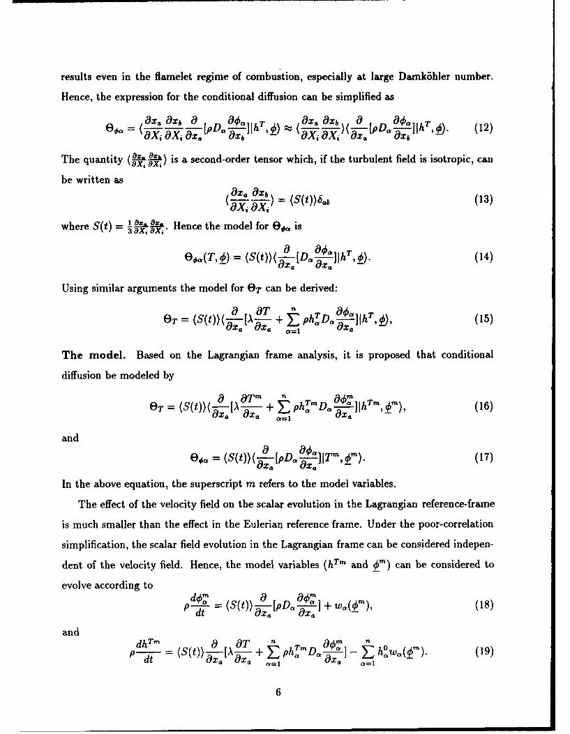
results even in the flamelet regime of combustion, especially at large Damk6hler number.

Hence, the expression for the conditional diffusion can be simplified as

[Ox. _xb 8 T aXa OXb 0 '00, TThe = - -i [ a)(W-'.-,-j-,h ,D_). (12)

The quantity _ of) is a second-order tensor which, if the turbulent field is isotropic, canOXi OXi

be written as0Xa = (13)

where S(t) = _._ Hence the model for O0 is3 8Xi OXi"

8#.(T, = (S(t))( a-[D -OŽ---lhT, 4,). (14)Za Oa aX

Using similar arguments the model for OT can be derived:O T " (15)h

OT =(S(t))( -a [T+ n phT D T (15)ax. Ox. •.=1 O- ,

The model. Based on the Lagrangian frame analysis, it is proposed that conditional

diffusion be modeled by

OT = (S(t))( [-P .+), (16)ax. a9x. 0 =1 Ox.

and

0. = (S(t))( -a[pD • TM] IOM). (17)xa O~aX -

In the above equation, the superscript m refers to the model variables.

The effect of the velocity field on the scalar evolution in the Lagrangian reference-frame

is much smaller than the effect in the Eulerian reference frame. Under the poor-correlation

simplification, the scalar field evolution in the Lagrangian frame can be considered indepen-

dent of the velocity field. Hence, the model variables (hTm and 0,') can be considered to

evolve according to40 = (S(t)) -0[pD 4901` (4+ ,(), (18)~dt Ox. ~OX

anddhTm a OT n O4" 11n

p dt = (S(t))-[A- + -hmD. ý '-O• how.(4_m ). (19)Ox a a=x O a • O1=1

6

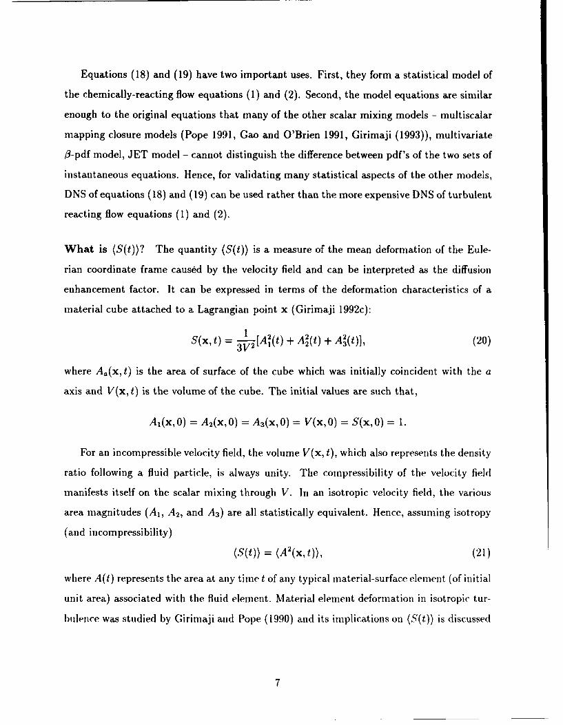
Equations (18) and (19) have two important uses. First, they form a statistical model of

the chemically-reacting flow equations (1) and (2). Second, the model equations are similar

enough to the original equations that many of the other scalar mixing models - multiscalar

mapping closure models (Pope 1991, Gao and O'Brien 1991, Girimaji (1993)), multivariate

03-pdf model, JET model - cannot distinguish the difference between pdf's of the two sets of

instantaneous equations. Hence, for validating many statistical aspects of the other models,

DNS of equations (18) and (19) can be used rather than the more expensive DNS of turbulent

reacting flow equations (1) and (2).

What is (S(t))? The quantity (S(t)) is a measure of the mean deformation of the Eule-

rian coordinate frame caused by the velocity field and can be interpreted as the diffusion

enhancement factor. It can be expressed in terms of the deformation characteristics of a

material cube attached to a Lagrangian point x (Girimaji 1992c):

S(x, t) = 1-[A2(t) + A2(t) + A2(t)], (20)

where Aa(x, t) is the area of surface of the cube which was initially coincident with the a

axis and V(x, t) is the volume of the cube. The initial values are such that,

A,(x,0) = A2(x,0) = A3(x,0) = V(x,0) = S(x,0) = 1.

For an incompressible velocity field, the volume V(x, t), which also represents the density

ratio following a fluid particle, is always unity. The compressibility of the velocity field

manifests itself on the scalar mixing through V. In an isotropic velocity field, the various

area magnitudes (A1 , A2, and A3 ) are all statistically equivalent. Hence, assuming isotropy

(and incompressibility)

(S(t)) = (A 2(x, t)), (21)

where A(t) represents the area at any time t of any typical material-surface element (of initial

unit area) associated with the fluid element. Material element deformation in isotropic tur-

bulence was studied by Girimaji and Pope (1990) and its implications on (S(t)) is discussed

7

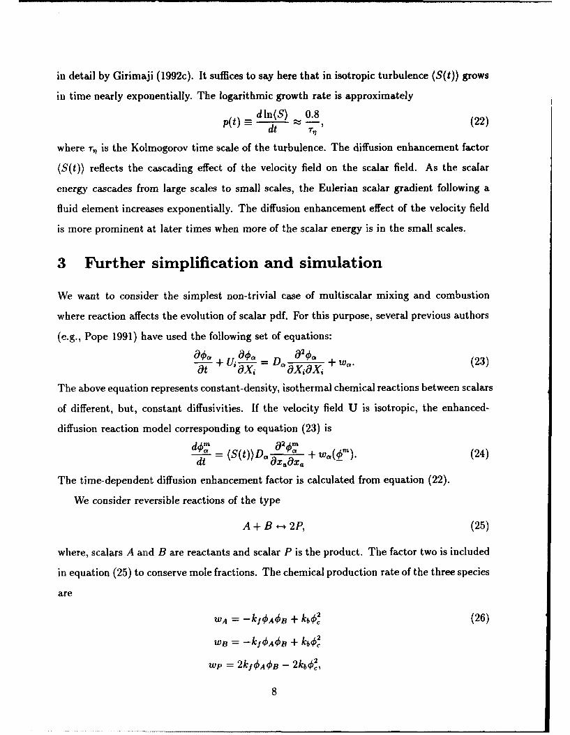
in detail by Girimaji (1992c). It suffices to say here that in isotropic turbulence (S(t)) grows

in time nearly exponentially. The logarithmic growth rate is approximately

dIn(S) 0.8 (22)p(t d = _-,

where r, is the Kolmogorov time scale of the turbulence. The diffusion enhancement factor

(S(t)) reflects the cascading effect of the velocity field on the scalar field. As the scalar

energy cascades from large scales to small scales, the Eulerian scalar gradient following a

fluid element increases exponentially. The diffusion enhancement effect of the velocity field

is more prominent at later times when more of the scalar energy is in the small scales.

3 Further simplification and simulation

We want to consider the simplest non-trivial case of multiscalar mixing and combustion

where reaction affects the evolution of scalar pdf. For this purpose, several previous authors

(e.g., Pope 1991) have used the following set of equations:

ao, + •,- = D " (23)

The above equation represents constant-density, isothermal chemical reactions between scalars

of different, but, constant diffusivities. If the velocity field U is isotropic, the enhanced-

diffusion reaction model corresponding to equation (23) is

dt - (S(t))OD, ' + w,(_m ). (24)

The time-dependent diffusion enhancement factor is calculated from equation (22).

We consider reversible reactions of the type

A + B " 2P, (25)

where, scalars A and B are reactants and scalar P is the product. The factor two is included

in equation (25) to conserve mole fractions. The chemical production rate of the three species

are

WA = -kf OA4B + kbOb2 (26)

WB = -kf -AOS + kbOS'

wp = 2kf ,AOB - 2kb40,

8

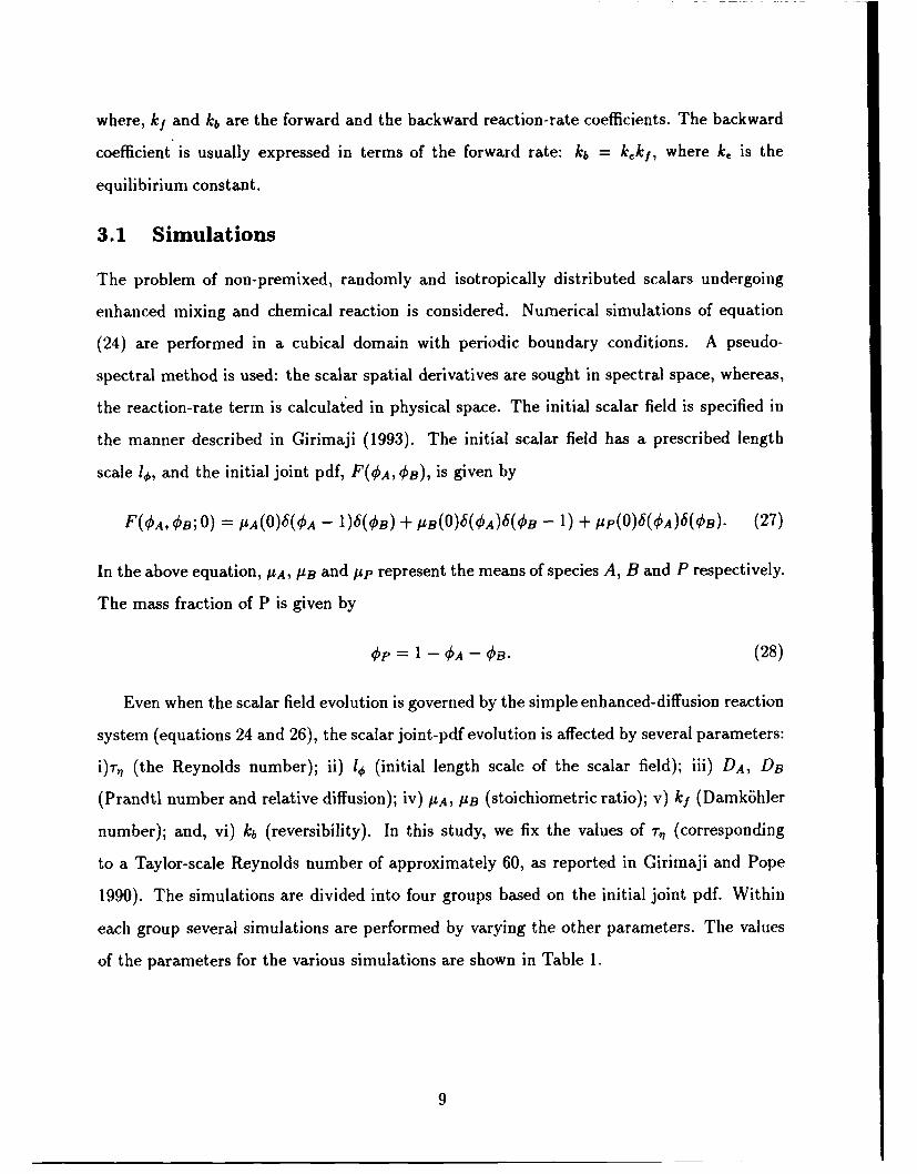
where, kt and kb are the forward and the backward reaction-rate coefficients. The backward

coefficient is usually expressed in terms of the forward rate: kb = kkf, where k, is the

equilibirium constant.

3.1 Simulations

The problem of non-premixed, randomly and isotropically distributed scalars undergoing

enhanced mixing and chemical reaction is considered. Numerical simulations of equation

(24) are performed in a cubical domain with periodic boundary conditions. A pseudo-

spectral method is used: the scalar spatial derivatives are sought in spectral space, whereas,

the reaction-rate term is calculated in physical space. The initial scalar field is specified in

the manner described in Girimaji (1993). The initial scalar field has a prescribed length

scale lj, and the initial joint pdf, F(OA, OB), is given by

F(OA, OB; 0) = (A(0)6(PA - 1)6(€B) + JB(0)6(OA)6(¢B - 1) + 1AP(0)6('A)6(¢B)- (27)

In the above equation, 'A, SB and Iup represent the means of species A, B and P respectively.

The mass fraction of P is given by

OP = 1 - OPA - OB. (28)

Even when the scalar field evolution is governed by the simple enhanced-diffusion reaction

system (equations 24 and 26), the scalar joint-pdf evolution is affected by several parameters:

i)-r (the Reynolds number); ii) l, (initial length scale of the scalar field); iii) DA, DB

(Prandtl number and relative diffusion); iv) IzA, ILB (stoichiometric ratio); v) kf (Damk6hler

number); and, vi) kb (reversibility). In this study, we fix the values of nr, (corresponding

to a Taylor-scale Reynolds number of approximately 60, as reported in Girimaji and Pope

1990). The simulations are divided into four groups based on the initial joint pdf. Within

each group several simulations are performed by varying the other parameters. The values

of the parameters for the various simulations are shown in Table 1.

9

4 Results and implications to turbulent combustionmodeling

The results of the simulations are presented in two parts. First, the effect of reaction on

the evolution of the means, variances, pdf's and other quantities of interest are studied.

Secondly, the simulation data are used in its role as the facsimilie of DNS to evaluate two

models of turbulent combustion: the mapping closure model and the assumed /3-pdf model.

The effect of chemical reaction on the follnwing statistics of various species are examined:

1. The mean, variances and correlations.

2. The evolution of the pdf.

3. The mean scalar dissipation and chemical production rate of variance.

4. The evolution of the conditional scalar dissipation.

Results from the simulations of Group 1 and Group 2 are used in this part of the study.

Statistics of species A and P only are presented, since OB can be completely determined

knowing OA and Op. In the discussions below, angular brackets imply mean and primes

denote fluctating part of a random variable.

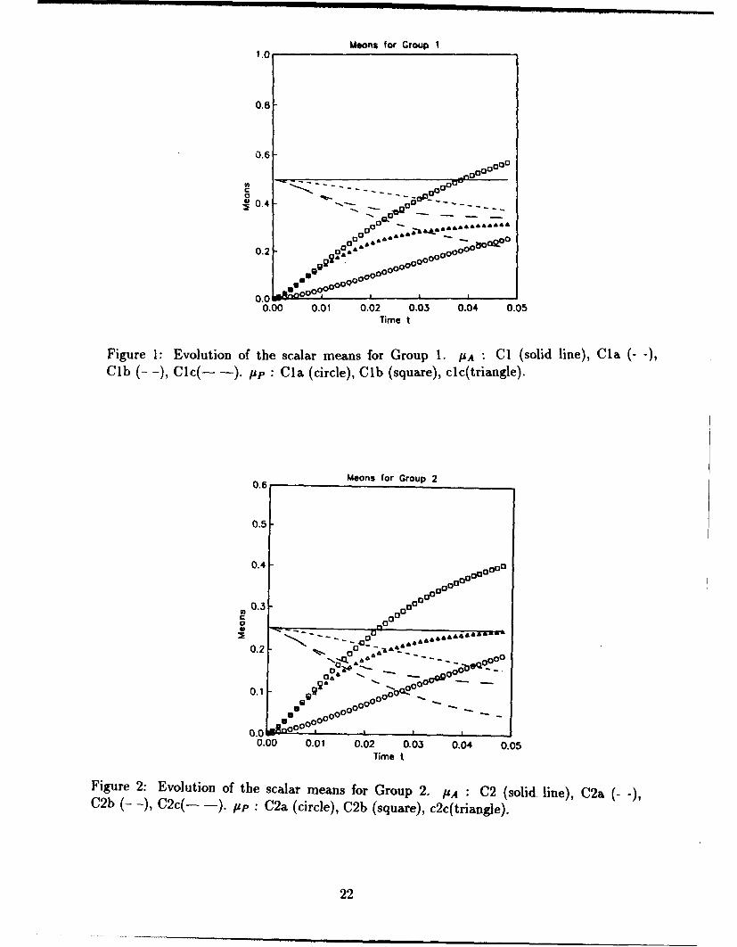
Means. The mean evolutions for Groups 1 and 2 are presented in Figures 1 and 2 respec-

tively. As is to be expected, the means do not change for the inert cases: (OA) remains at its

initial value, and (Obp) is always zero. As for the reacting cases, the mean reactant decreases

more rap.dly for larger k! (reaction rate coefficient) than for smaller kf. In the reversible

reaction cases (CIb and C2b), the mean values asymptote to equlibrium values given by the

equation

PAYB = IPI, (29)

The above equation in conjunction with equation (28) leads to the following equlibrium

values: for case Clb, 11A = 0.33, PB = 0.33, pp = 0.33; and for case C2b, PA = 0.116, PB =

0.616, pp = 0.267.

10

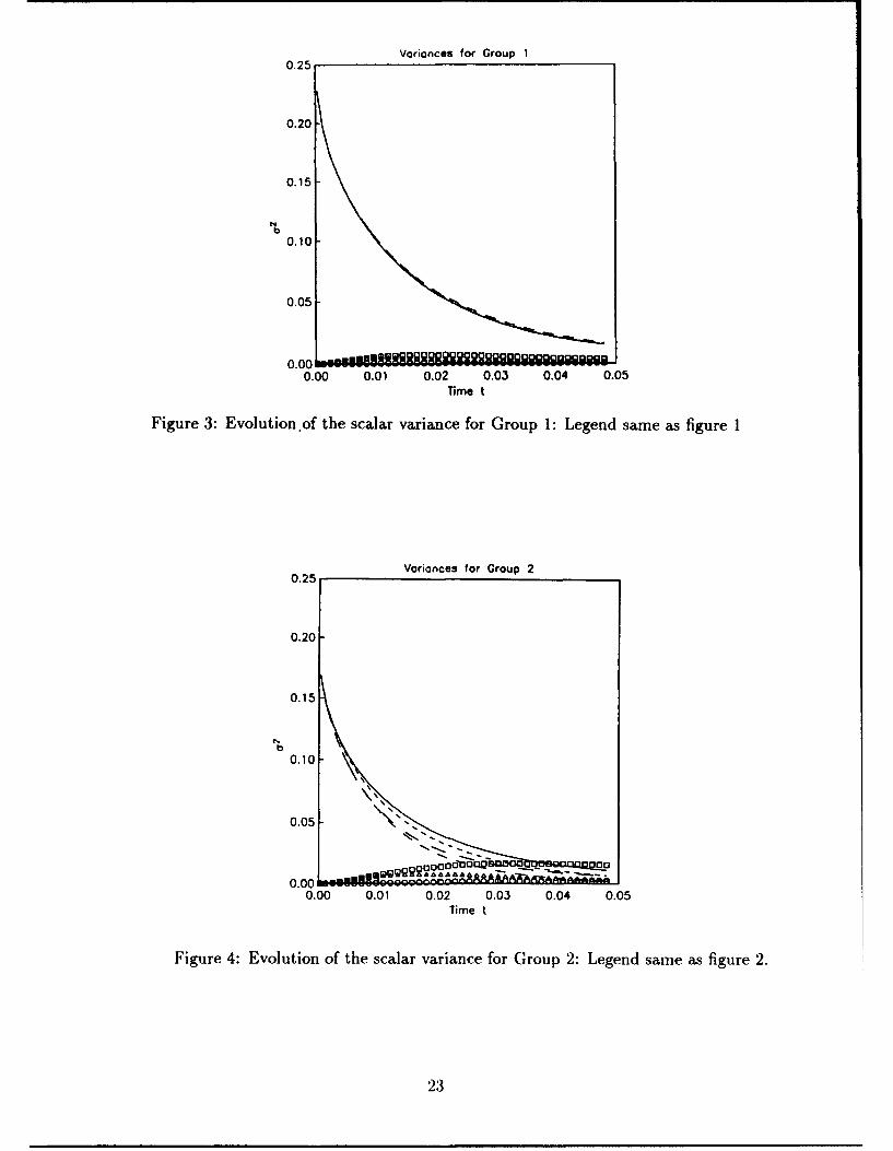
Variances. The evolution of variance in reacting field in given by

do,._dt - + (30)dt

where, the mean scalar dissipation (c) and the production/destruction of variance due to

reaction (e,) are defined as

fa = ax, (31)

41= (wo~ko). (32)

The variances of species A for Groups 1 and 2 are shown in Figures 3 and 4. In Group 1,

reaction appears to cause the variance to decay slowly compared to the inert case. On the

contrary, in Group 2, the variance decays more rapidly with reaction than without. The effect

of reaction on Group 2 is larger than that on Group 1. The reasons for these observations

are explained further below, when the behavior of f is discussed. Although discernable,

the magnitude of the modification due to reaction is small enough to be unimportant for

practical problems. As shown in Figures 6 and 7, c d> Er for the cases considered resulting

in only a slight modification of the variance evolution.

The variance of the product is initially zero. It grows in time initially, due to the chemical

production term; more rapidly in Group 2 than in Group 1. After attaining a peak value, it

diminishes due to effect of molecular action.

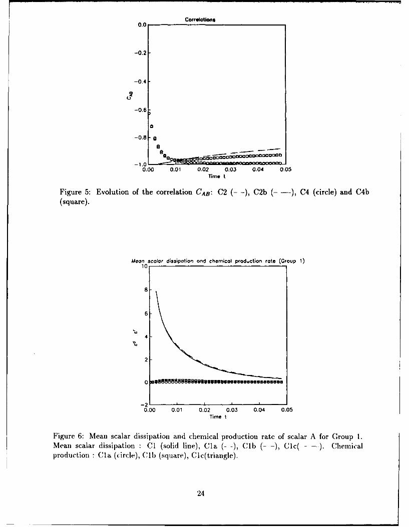
Correlation between OA and OB. The correlation coefficient between species A and B,

CAB A B (33)2a2'

UOA ~B

is given in Figure 5 for the inert cases C2 and C4 and their reacting counterparts C2b and

C4b. At early times, when chemical conversion is small, correlation is not affected much

by chemical reaction. With time the correlation for the reacting cases deviate from their

inert counterparts, going to lower magnitudes while still preserving a negative sign. The

deviation, however, is not too large.

11

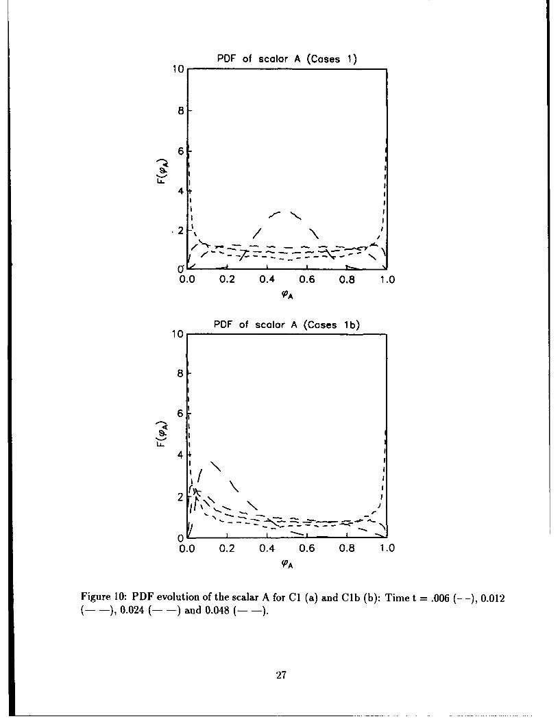
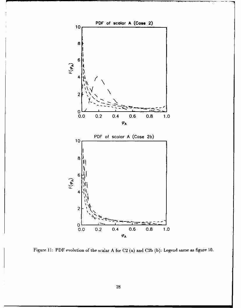
Scalar pdf. In order to examine the effect of reaction on the scalar pdf evolution, the pdf

of scalar A is plotted in Figure 6 for cases C1 and Clb. Figure 7 contains pdf's of scalar A

for cases C2 and C2b. Initially, chemical reaction does not affect the pdf much, for, given the

segregated initial condition, molecular mixing should occur first before chemical conversion.

However, at later stages, as chemical conversion becomes prevalent, the pdfs are strongly

affected. The pdf's develop positive skewness due to chemical depletion, and in both cases

tend to b-functions at zero at long times.

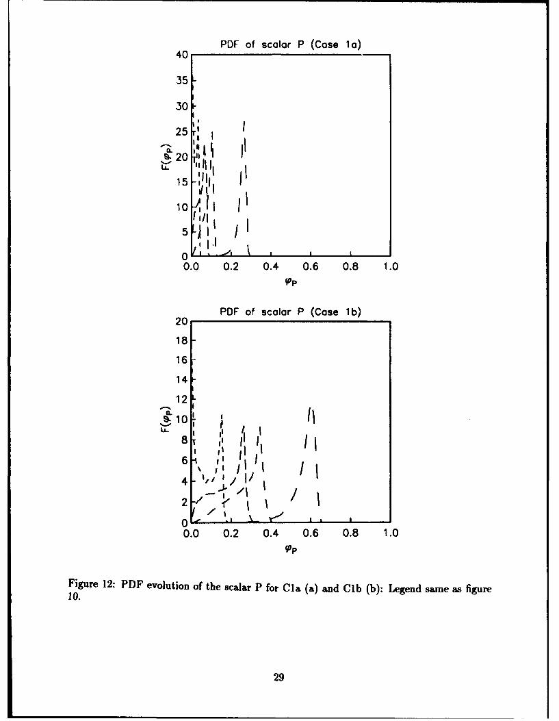
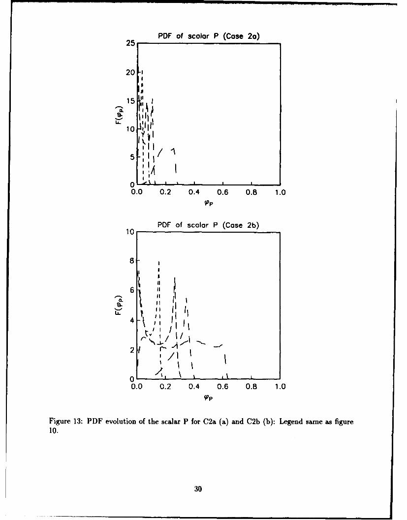
The pdf of the product, scalar P, is plotted in Figure 8 (Cases Cla and Clb) and Figure 9

(Cases C2a and C2b). The pdf's of both groups display bimodal behavior initially. One mode

of high probability is at zero value of mass fraction, representing parts of the field containing

unmixed reactants. The second mode of high probability is close to the maximum value of

mass fraction at that time. With time, the mode at zero disappears, and the other mode

migrates to higher values retaining its spike-like form, in cases Cla and Clb. The asymptotic

state of the pdf for Group 1 is a M-function at unity, representing a complete conversion of

all reactants to products. In cases C2a and C2b also the mode at zero dissipates with time.

The pdf migrates to the right and has wider support (larger variance) unlike Cla and Clb.

The asymptotic form of the pdf in these cases (Group 2) is a 6function at Op = 0.5.

Chemical production-rate of variance. The chemical production-rate of variance of

species A is given by

-=" -- ((AwWAB) -- (OB)(4•') - ('AO'AO4B)• (34)

For Groups 1 and 2, the correlation between A and B is nearly negative unity leading to

OA ;-Z' _4(35)

which when substituted in equation (34) leads to

= (w¢'A) = [(OA) - (OB)](0'0') + (q•). (36)

Similar arguments lead to

= (W•'B') = [(qSR ) - (0A)](0B0'B) + (4B)" (37)

12

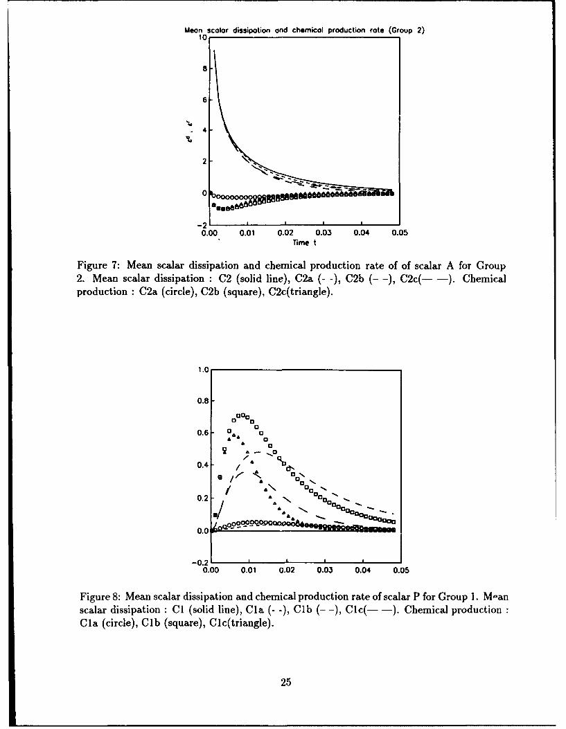
In Figures 10 and 11, e" of Groups 1 and 2 are presented. The behavior of f in the two

groups can be understood by recalling that for Group 1, (phiA) = (OB) and for Group 2,

(OB) = (A) + 0.5, at all times. This yields

C (38)

for Group 1. As mentioned earlier, the pdf is positively skewed leading to a positive value

for c. For Group 2

r :, -0.5(phi2) + (c). (39)

For this group, the first term on the right hand side (of equation 39) dominates the skewness

term leading to a larger negative value of f. The behavior of the variances of the two groups

is consistent with the above explanations.

Figures 12 and 13 contain f, of groups 1 and 2. Both groups exhibit similar behavior.

Starting from zero, the value of f, increases to a peak value and then diminishes to near-zero

values. The peak value is higher for higher kf. The early behavior of e of the reversible

case is identical to its non-reversible counterpart. However, its peak value is not as high,

and it diminishes much more rapidly to zero.

Mean scalar dissipation. The mean scalar dissipation of species A of Groups I and 2

are given in Figures 10 and 11. Similarly to its effect on variance, reaction causes the mean

scalar dissipation to decay more slowly in Group 1 and more rapidly in Group 2. Again,

the magnitude of modification is not very large. In both groups, the magnitude of the mean

scalar dissipation is much larger than that of chemical production-rate of scalar variance.

The mean scalar dissipation of P of Groups 1 and 2 are given in Figures 12 and 13. In

both the groups., with the formation of products, the mean scalar dissipation increases from

a zero initial value. After attaining a maximum value, the dissipation decreases. The mean

scalar dissipation achieves higher values in Group 2 than the corresponding cases in Group

1. Initially, c, is larger in magnitude than f,, leading to a growth of ap2 from its initial zero

value. At latter times, fd is larger leading to a decay in the variance levels. The implication

is that initially the scalar-P evolution is reaction controlled, after which both reaction and

diffusion are equally important, and ultimately the evolution is diffusion controlled.

13

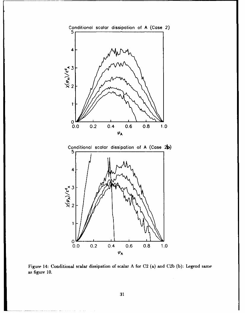
Conditional scalar dissipation. The evolution of the conditional scalar dissipation of

scalar A in cases C2 (inert) and C2b (reacting) is given in Figure 14. Chemical reaction

has two effects on this quantity. The first is due to the more rapid decline in the maximum

value of OA as a result of reaction. The zero of the conditional dissipation migrates with the

extremum value (Girimaji 1992b). When mixing is accompanied by reaction, the conditional

dissipation is non-zero over a smaller range of OA, than in the case of inert mixing. This

effect is negligible at the early stages and more pronounced in the later stages. The second

difference is the higher value of the conditional dissipation (where it is non-zero) at a given

value of mass fraction in the reacting case as compared to inert case. Again, this difference

is large in the latter stages and negligible in the early part. Despite the higher values of

the conditional scalar dissipation in the reacting case than in the inert case, the mean scalar

scalar dissipation is indeed lower in the reacting case, as shown in Figure 11. The reason for

this is the shift in the pdf (Figure 11) due to reaction. In the reacting case, the high values

of conditional dissipation occur at values of mass fraction of low probability of occurence

and vice versa. Whereas, in the inert case high probability and high conditional dissipation

appear to occur at nearly same values of mass fraction.

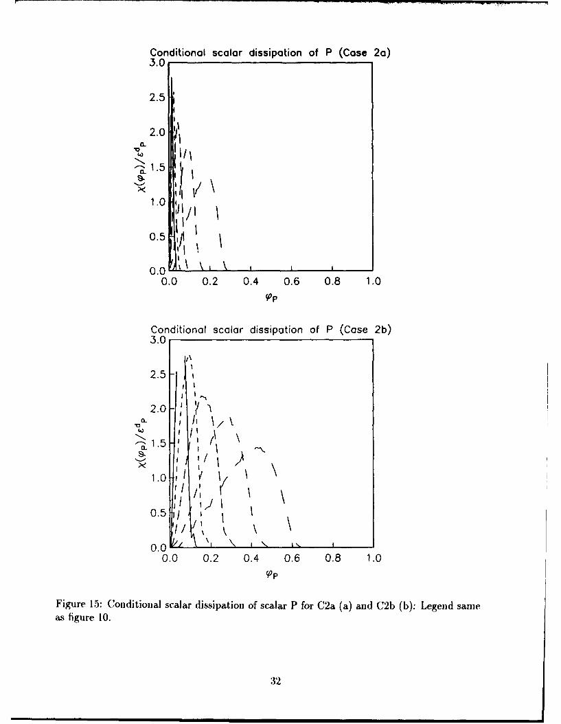
The conditional scalar dissipation of the product, scalar P, is given in Figure 15 for cases

C2a and C2b. The conditional dissipation of the product is very unlike that of the reactant

for this case. Initially, it is non-zero over a very narrow range of Op values and it gradually

widens with time (or reaction). The peak value normalized by the mean scalar dissipation

decreases with time, indicating gentler gradients in the product field at later times. The

behavior of this quantity is further discussed later when the modeling issues are examined.

So far in this section, the effect of reaction on various quantities of interest was examined.

It is found that although the mean and pdf of the scalars are strongly affected by reaction,

other quantities like the variance (and, perhaps, other even moments) are not very different

from their inert-mixing counterparts. Hence, it would be useful to directly compare and

evaluate models of inert mixing against the enhanced-diffusion/reaction data.

14

4.1 Models vs. Data

We attempt to answer three specific questions regarding turbulent combustion modeling

using other models:

1. Can the inert mixing multiscalar mapping-closure model (Girimaji 1993) be used for

reacting flows without modification?

2. How good is the multivariate assumed fl-pdf model (Girimaji 1991a) for calculating

reacting flows?

3. How does the computationally simple assumed-pdf model compare with mapping-

closure model for multiscalar mixing?

Multiscalar mapping closure model. The multiscalar mapping closure model for inert

mixing (Girimaji 1993) is based on the simplification that the conditional scalar diffusion of

a given scalar is a function of that scalar only:

044 = ( t -[D•-• ,1T,_) ; -z (a[D ý-1]JT•.)- (40)

The conditional scalar diffusion for each scalar is obtained by employing the mapping closure

procedure for single scalar mixing. Knowing the conditional scalar diffusion of each scalar,

the joint pdf evolution is solved, and the results are in reasonably good agreement with data.

Even when mixing is accompanied by reaction, it is suggested in Girimaji (1993) that

the simplification stated in equation (40) may be valid. In the reacting case, however, the

mapping closure procedure even for single scalar is not clear. So it will be useful to know, if

the condiJ,>, al scalar diffusion implied by the mapping closure procedure for inert mixing is

adequate for the reacting case also. Conditional scalar diffusion is related to the conditional

scalar dissipation accor aiig tc

(41O = F(1 dxF(,~ (41)

The inert case mapping closure model (with Gaussian reference field) for conditional scalar

dissipation for initially non-premixe,4 reactants is (Girimaji 1992b)

X(=) _exp(-2[erf-'f{2 - 1}]2). (42)

15

This model is quite good in the early stages of inert mixing and is technically invalid but

still adequate during the latter stages. The validity of the above model for the reacting case

is now investigated.

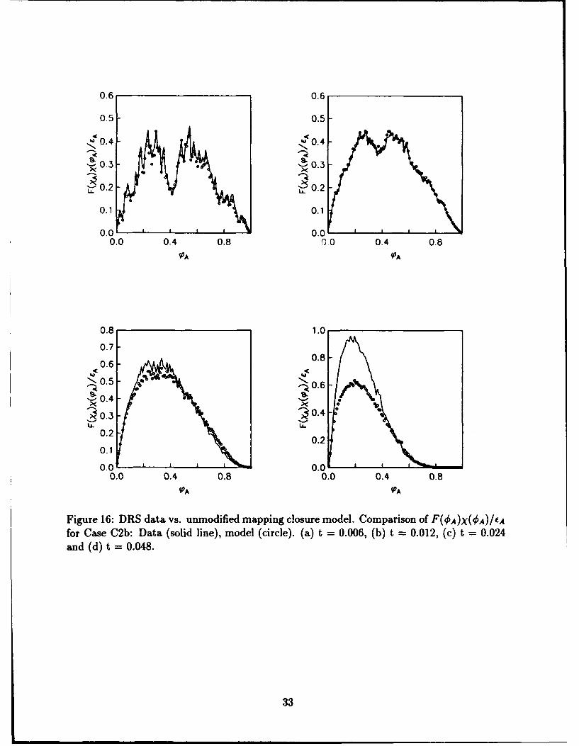
Shown in Figure 16, are F(OA)X(4PA)/X(ObA = 0.5) of the data and model for case C2b.

In the model calculation of the above quantity, pdf F is taken from the data. The model

agrees with the data very well at early times. At later times, the model is still adequate.

Recall that even for the case of inert mixing the model is not very good at the final stages.

Perhaps, an inert-case model which is uniformly valid at all times would be good for reacting

case at all times too. In any event, for combustion applications, the behavior of the model

at the early stages, when the unmixedness is high, is more important than at the late stages

when the scalars are more or less uniformly mixed. Hence, for the reactants a closure model

for the conditional scalar diffusion obtained by substituting equation (42) in equation (41)

might be adequate.

Modeling the conditional diffusion of the product (scalar P) is not as simple. The relative

importance of chemical conversion and mixing in the scalar pdf evolution (of P) at various

times can be surmised from Figure 9 where the mean scalar dissipation and the chemical

production rate of variance are compared. Initially, the evolution of the scalar P is dom-

inated by chemical conversion. Molecular diffusion does not play a significant role in the

pdf evolution until much later. Therefore, it is important that the model for the conditional

diffusion (or dissipation) of the product be accurate at later times; accuracy at early times is

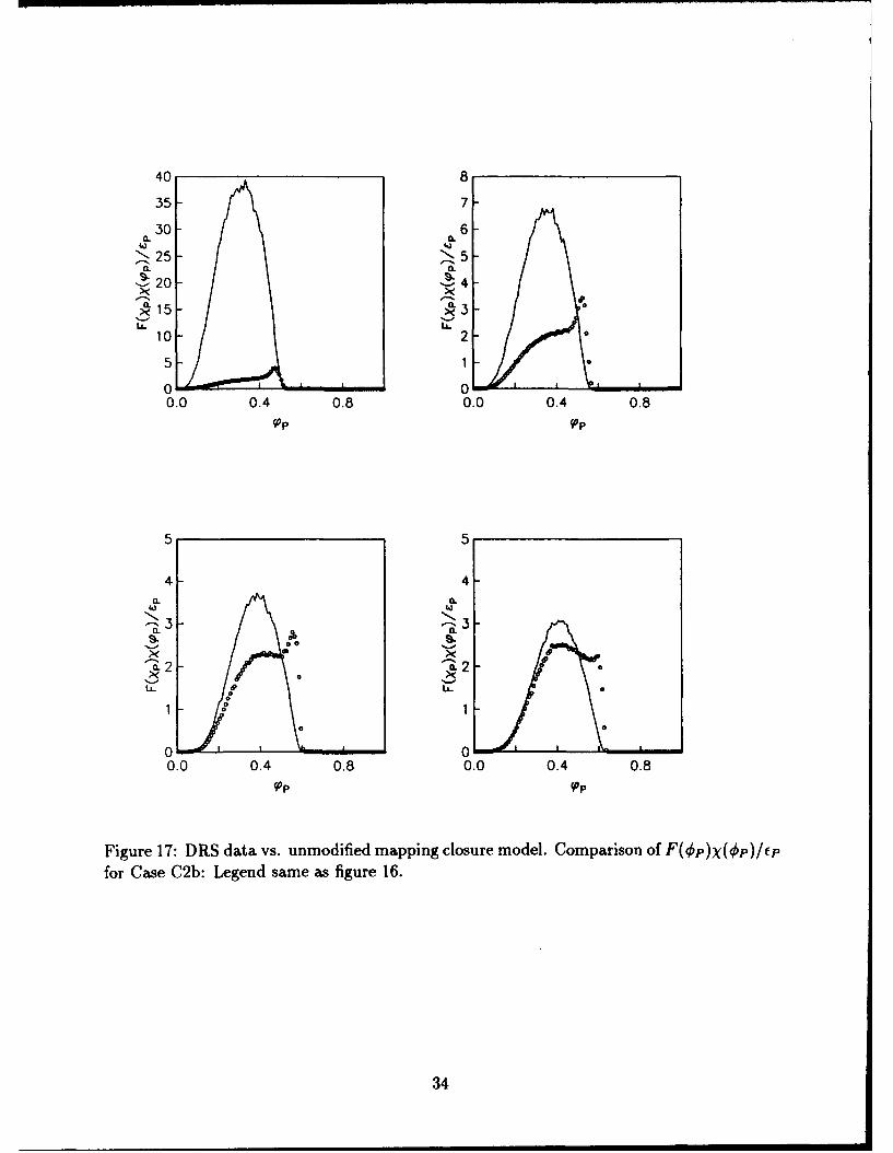
not as crucial. Comparison of F(lop)X(op)/X(Oep = 0.5) for the product is shown Figure 17

for case C2b. The agreement is very poor in the initial stages. At the later stages, it is much

better. Whether the model is good enough for engineering applications can be determined

only from the computation of the pdf evolution using the closure model. Such a computation

is outside the scope of this work.

Assumed multivariate /-pdf model. In the assumed-pdf approach the scalar joint pdf

is prescribed knowing the first few moments of the scalar field. It is computationally far less

intensive than the mapping closure model and is ideally suited for engineering computations.

16

The assumed multivariate • pdf model for a N-scalar mixing process is given by (Girimaji

1991a)

)=r(fi1 +--..+ fN) 1 1 -1 -I""" .-6(l -- - -e2N). (43)rF~f) =)'

The parameters of the model ( ON,'", /N) are functions of the mean mass fractions p and

turbulent scalar energy Q:A( 1 - 1). (44)

In the above equation Q and S are given by

N N

Q =- Eu 2 ; S = P• 2 . (45)

where a' is the variance of mass fraction of scalar a. The above model tested for two-scalar

inert mixing process with reasonable success, but is yet to be validated for multiscalar mixing

and reaction.

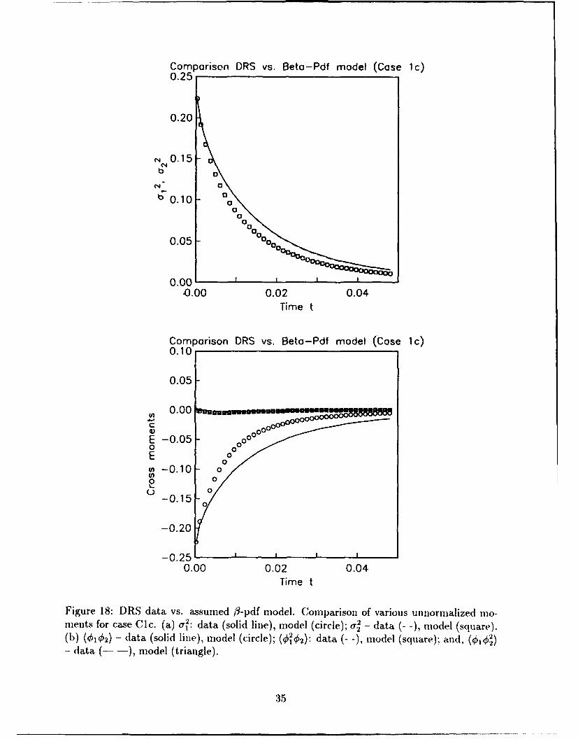
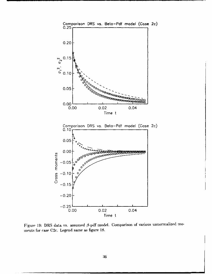
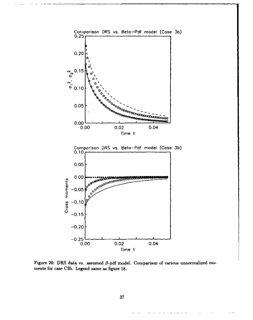
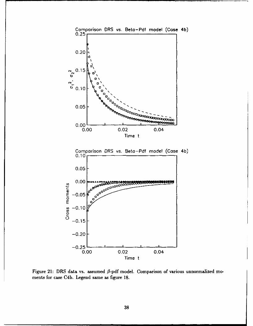
In Figure 18, the individual variances and some cross moments of species A and B cal-

culated using the model are compared against corresponding simulation data for case Clc.

Similar comparisons are performed for cases C2c, C3b and C4b in Figures 19, 20 and 21,

respectively. The means and the turbulent scalar energy required as inputs to the model are

taken from DRS data. The model predicts the variances reasonably well. The magnitude of

the cross covariance is consistently underpredicted by the model, but the difference is not too

much. For the two higher order cross moments compared ((020' ) and (0' 0')) the model

does surprisingly well. For each of the cases considered, the moments behave differently and

the model is able to capture the behavior well, qualitatively and quantitatively. Overall the

performance of the model is quite satisfactory, given the simplicity of the model.

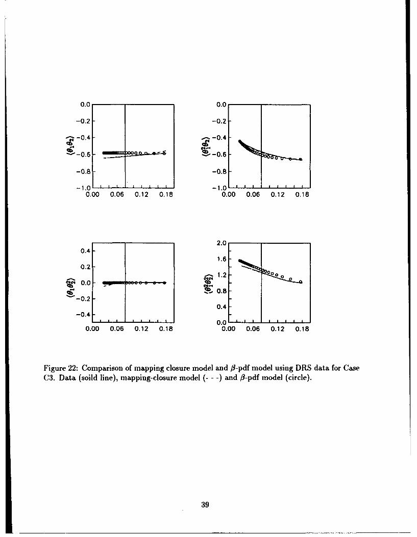
Multivatiate 03-pdf model vs. Mapping closure model. Now the assumed /3-pdf

model is compared against the more detailed and computationally intensive mapping closure

model. The two models are equally good for the case of inert non-premixed two scalar

mixing (Girimaji 1992b). Comparison of the two models for multiscalar mixing has not

been performed before, and is attempted presently for inert mixing. (As mentioned before,

computations of multiscalar reacting flows using mapping-closure model are intensive to be

17

attempted here.) For the purpose. of computation, simulations C3 and C4 are used. In the

absence of reaction, Groups 1 and 2 reduce to two-scalar mixing, and hence not useful to

evaluate multiscalar. In Figure 22, various normalized cross moments (of species A and B)

obtained from the simulations are plotted as a function of the variance of scalar A for Case

C3. (The variance decreases monotonically in time and hence can be used in lieu of time

as the abcissa.) Also shown in the Figure are the cross moments calculated using the two

models. The moments of the normalized variables are presented:

0_ = 0. (P_) (46)

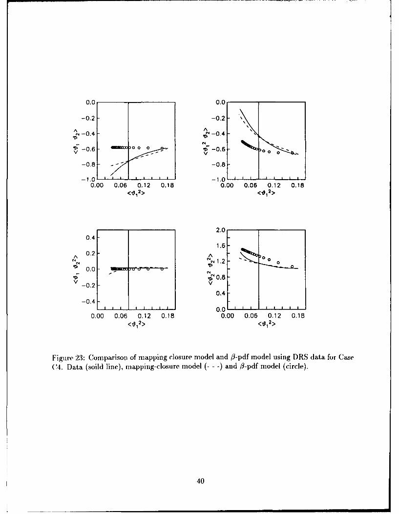
For all the moments considered, both the models agree equally well with the data. Figure

23 presents the same comparison for case C4. In this case, the performance of the mapping

closure model is clearly superior. These findings are in keeping with the arguments presented

in Girimaji (1991a) that the assumed /-pdf model is likely to be more accurate when the

length-scale and diffusivities of the scalars are similar (case C3) than when they are widely

disparate (case C4). For case C4, even the mapping closure model is not very accurate. This

leads to the question, for engineering calculations, is the increase in accuracy achieved using

the mapping closure model worth the extra effort involved in computing? The answer will

depend on the application for which the model is being used. In combustion calculations it

is the unnormalized moments that appear in the scalar moment equations and need closure

modeling, not the normalized moments. Despite the relatively poor agreement of the nor-

malized moments in Figure 23, the unnormalized moments calculated using the f-pdf model

are quite close to the data as seen in Figure 21 for the corresponding reacting case C4b.

This appears to suggest that the assumed-pdf approach, although simplistic, may be quite

adequate for modeling of turbulent combustion in engineering calculations.

5 Conclusion

It is shown that in isotropic turbulence the (enhanced) diffusion-reaction system (18 and

19) can be considered a statistical model of turbulent combustion (equations 1 and 2) with

the initial field and the diffusion enhancement factor ((S(t))) as inputs. The diffusion-

enhancement factor can be found if the scalar variance evolution is known (Girimaji 1992c).

18

In the event that scalar variance evolution is not known from any other source, a simple

model for the diffusion-enhancement factor is provided (equation 22). The enhaaced-diffusion

reaction model is close enough to the turbulent combustion equations that, in normalized

time, many of the other models (mapping closure models, assumed-pdf models and any

model that decouples the velocity and scalar fields) cannot distinguish between the present

model and the original equations.

Simulations of the diffusion-reaction system is performed in a cubical box (64' grid points)

from non-premixed initial conditions. The reaction considered is of the type

A+B -B P.

The reaction is constant-derisity and cold (isothermal). Several simulations of different initial

conditions, reaction-rate coefficient and degree of reversibility are performed (Table 1). The

simulations are used to examine the effect of reaction on the evolution of several scalar

staistics (Figures 1 - 15). The data are also used to evaluate other models; mapping closure

model and the assumed multivariate /3-pdf model. The observations and inferences from the

study are the following.

1. The conditional scalar dissipation implied by the inert mapping closure model is rea-

sonable even for reacting case but only for the reactants (scalars A and B) as shown in

(Figure 16). For the product (scalar P), the agreement is quite poor at early times but

better at later times (Figure 17). Since, the evolution of scalar P is initially dominated

by chemical conversion and not molecular mixing, the accuracy of the conditional dis-

sipation model at the early stages may not be critical to the overall performance of the

model. At the later stages, when the evolution of scalar P is mixing dominated, the

model is adequate. For this reason, the use of equations (42 and 41) as closure model

may yet yield reasonable results.

2. A close comparison (of the normalized moments) of the multiscalar mapping closure

model and the multivariate #-pdf model (Figures 22 and 23) against inert data shows

that the two models are quite close when the initial length scales and diffusivities

19

are similar. The mapping closure model is superior when those parameters are vastly

different for the different scalars.

3. The assumed f-pdf model comes reasonably close in calculating many of the unnor-

malized moments of the scalar joint pdf, even for the reacting case and even when

the initial length scale and diffusivities of the participating scalars are quite disparate

(Figures 18 - 21). It is the unnormalized moments that require closure modeling in tur-

bulent calculations. Hence, despite the disagreement of the normalized moments under

some circumstances, the assumed 83-pdf model appears to be adequate for engineering

calculations.

References

[1] Chen, H., Chen, S. and Kraichnan, R. H. (1989) Probability distribution of a stochasti-

cally advected scalar field. Physical Review Letters, 63 (24), 2657 - 2660.

[2] Eswaran, V., and Pope, S. B. (1988) Direct Numerical Simulations of the turbulent

mixing of a passive scalar. Physics of Fluids, 31 (3), 506 - 520.

[3] Gao, F. (1991) Mapping closure for multispecies Fickian diffusion. Phys. Fluids 3 (10),

2438 - 2444.

[4] Girimaji, S. S. and Pope, S. B. (1990) Material element deformation in isotropic turbu-

lence J. Fluid. Mech. 220, pp 427 - 458.

[5] Girimaji, S. S. (1991a) Assumed 3-pdf model for turbulent mixing: validation and ex-

tension to multiple scalar mixing. Combust. Sci. and Tech. 78, 4 - 6, 177 - 196.

[6] Girimaji, S. S. (1991 b) A simple recipe for modeling reaction rates in flows with turbulent

combustion. AIAA-91-1792. AIAA 22nd Fluid Dynamics, Plasma Dynamics and Lasers

Conference, June 24-26, 1991, Honolulu, Hawaii.

[7] Girimaji, S. S. (1992a) A mapping closure for turbulent scalar mixing using time-evolving

reference field. Phys. Fluids A (in press).

20

[8] Girimaji, S. S. (1992b) On the modeling of scalar diffusion in isotropic turbulence. Phys.

Fluids. A, 4 (11), 2529 - 2537.

[9] Girimaji, S. S. (1992c) Towards understanding turbulent scalar mixing. NASA Contract.

Rep. CR 4446.

[10] Girimaji, S. S. (1993) A study of multiscalar mixing. Phys. Fluids. A, 5 (7), 1802 - 1809.

[11] Madnia, C. K., Frankel, S. H., and Givi, P. (1992) Reactant conversion in homoge-

neous turbulence: mathematical modeling, computational validations and practical ap-

plications. Theoret. Comput. Fluid Dynamics, 4, 79 - 93.

[12] Kerstein, A. R. (1988) A linear eddy model of turbulent scalar transport and mixing.

Combust. Sci. and Tech., 60, 391 - 421.

[13] Pope, S. B. (1985) PDF methods for turbulent reacting flows. Prog. Energy Combust.

Sci., 11, 119- 192.

[14] Pope, S. B. (1991) Mapping closures for turbulent mixing and reaction. Theo. and Comp.

Fluid Dynamics, 2, 255 - 270.

[15] Williams, F. A. (1988) Combustion Theory. Addison - Wesley Publishing Company,

Inc., New York.

21

Moons for Group 1

1.0

0.8

0.6

_r1 n0000

00

0.2 0a

111169 12. 000OoOO OO000000 0 0 -

low oooooo

0.o011 oo6 a , ,0.00 0.01 0.02 0.03 0.04 0.05

Time t

Figure 1: Evolution of the scalar means for Group 1. /.A : CI (solid line), Cla (- -),Clb (- -), Clc(--). up: Cla (circle), Cib (square), clc(triangle).

Means for Group 2

0.6

0.5

0.4 030000

00101330

r-00

C-

0.2 " a - #00

0000000

000000 -.

0.1 00 00000 0 0 -

a: ; o o 0- ---Oo oci0.00 0.01 0.02 0.03 0.04 0.05

Time t

Figure 2: Evolution of the scalar means for Group 2. PA : C2 (solid line), C2a (- -),C2b (--), C2c(- -). yp : C2a (circle), C2b (square), c2c(triangle).

22

Varionces for Group 1

0.25

0.20

0.15

%

0.10

0.05 -

0.00 Lgloesii

0.00 0.01 0.02 0.03 0.04 0.05

Time t

Figure 3: Evolution.of the scalar variance for Group 1: Legend same as figure 1

Vorionces for Group 20.25

0.20

0.15

b0.10

0.05

0.00 0.01 0.02 0.03 0.04 0.05Time t

Figure 4: Evolution of the scalar variance for Group 2: Legend same as figure 2.

23

Correlations

0.0

-0.2

-0.4

-0.6

-0.8 a

*~oga m~aoaoaoaaoaoaooaaaaa"- 1.0 ".80M "0003O,,OOJM

0.00 0.01 0.02 0.03 0.04 0.05Time t

Figure 5: Evolution of the correlation CAB: C2 (- -), C2b (- -- ), C4 (circle) and C4b(square).

Mean scaJer dlssipotion and chemical production rote (Group 1)10

8

6-

4

2

c sube5BBBe8UUUUluuuueoelueeueeoeeuooooueo

-2 |0.00 0.01 0.02 0.03 0.04 0.05

Time t

Figure 6: Mean scalar dissipation and chemical production rate of scalar A for Group 1.Mean scalar dissipation : CI (solid line), Cla (--), Clb (--), Clc(- -). Chemicalproduction : Cla (circle), CIb (square), Clc(triangle).

24

Mean scalar dissipation and chemical production rate (Group 2)

10

8

6

4

O'oooo 2 Bass"~A ---

-20.00 0.01 0.02 0.03 0.04 0.05

Time t

Figure 7: Mean scalar dissipation and chemical production rate of of scalar A for Group2. Mean scalar dissipation : C2 (solid line), C2a (- -), C2b (- -), C2c(- -). Chemicalproduction C2a (circle), C2b (square), C2c(triangle).

1.0

0.8

000

00.6 o %

& 0

0 .4 / &£0

g A 0 •.

/ 000%-o0.2 / N. 0o0 . •

£0 0000

0.0 1o69 ---.. .

-0.21mm0.00 0.01 0.02 0.03 0.04 0.05

Figure 8: Mean scalar dissipation and chemical production rate of scalar P for Group 1. Mpanscalar dissipation : CI (solid line), Cla (- -), Clb (- -), Clc(- -). Chemical productionCla (circle), Clb (square), Clc(triangle).

25

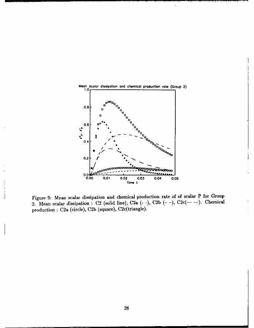
Mean scalar dissipation ond chemical production rate (Group 2)1.0

0.8- 0 0C000 000O 00.8 o 0%

0 0

0

V 0

a

00

0.6 o2 0*°0

00 0000

0.00 0.01 0.02 0.0, 0.04 0.05

Time t

Figure 9: Mean scalar dissipation and chemical production rate of of scalar P for Group

2. Mean scalar dissipation : (C2 (solid line), (32a (- -), (32b -),(2c(----). C3hemical

production : (32a (circle), (32b (square), (32c(triangle).

26i

PDF of scalar A (Cases 1)

10

8

6

4

0.0 0.2 0.4 0.6 0.8 1.0VPA

10 PDF of scalar A (Cases 1 b)

8

6

4

/

0 I - 1 - -

0.

0.0 0.2 0.4 0.6 0.8 1.0

VPA

Figure 10: PDF evolution of the scalar A for CA (a) and Cs b (b): Time t .006 0.012

( -- ,0.024 (- -)and 0.048(- - .

27

PDF of scolor A (Case 2)10

8

6

4

2 x>

0 p I'-- --

0.0 0.2 0.4 0.6 0.8 1.0V0A

PDF of scolor A (Case 2b)10

8

6J• ',lI

4 ."

2

0.0 0.2 0.4 0.6 0.8 1.0VOA

Figure 11: PDF evolution of the scalar A for C2 (a) and C2b (b): Legend same as figure 10.

28

40 PDF of scolor P (Cose 1 a)

35

30

25 r'

%S-20U-15

10

5

O[i0.0 0.2 0.4 0.6 0.8 1.0

(P p

20 PDF of scolar P (Cose 1 b) -

18-

16

14

12

10U-

8 T

6

4 -

2

00.0 0.2 0.4 0.6 0.8 1.0

p

Figure 12: PDF evolution of the scalar P for Cla (a) and Clb (b): Legend same as figure10.

29

PDF of scolor P (Case 2o)25

20 L-ISN

15 1

10 ,

5A I

0.0 0.2 0.4 0.6 0.8 1.0Vp

PDF of scalor P (Case 2b)10

8 -

III6

'I

2

010.0 0.2 0.4 0.6 0.8 1.0

Figure 13: PDF evolution of the scalar P for C2a (a) and C2b (b): Legend same as figure10.

30

Conditional scalar dissipation of A (Case 2)

5

4-

1-

00.0 0.2 0.4 0.6 0.8 1.0

W#A

Conditional scalar dissipation of A (Case 2b)5

4-

V<c 3

x 2

1

00.0 0.2 0.4 0.6 0.8 1.0

W#A

Figure 14: Conditional scalar dissipation of scalar A for C2 (a) and C2b (b): Legend sameas figure 10.

31

Conditional scalar dissipation of P (Case 2a)3.0

2.5

2.0 1

1.0X/I '.

0.5 '•

0.00.0 0.2 0.4 0.6 0.8 1.0

DP

Conditional scalar dissipation of P (Case 2b)

3.0

2.5

2.0 "

. 1.5 -/ "'

1.0 I V

0.5 ,I,\

0.00.0 0.2 0.4 0.6 0.8 1.0

'Pp

Figure 15: Conditional scalar dissipation of scalar P for C2a (a) and C2b (b): Legend sameas figure 10.

32

0.6 0.6

0.5 0.5

.0.4- 0.4

03 - 0 o.30X

• 0.2 0.2

0.1 0.1

0.0 0.00.0 0.4 0.8 0 0 0.4 0.8

WA VA

0.8 1.0

0.70.6 -0.8-

0. 5 - N .-0.8-

0.64 -0.06

LA.

0.2

0.10.

0.0 0.00.0 0.4 0.8 0.0 0.4 0.8

WA VA

Figure 16: DRS data vs. unmodified mapping closure model. Comparison of F(qOA)X(qSA)/1A

for Case C2b: Data (solid line), model (circle). (a) t = 0.006, (b) t = 0.012, (c) t = 0.024and (d) t = 0.048.

33

40 8

35 7

30 6

>25 5-a. a.

--- 20 -. 4X~ k

A'15 )3 0

LA- La..10 2

5 1 0

0 , 00.0 0.4 0.8 0.0 0.4 0.8

5 5

4 - 4 -0. a.

-3 -3a.

00

0 00

1 - 100 0

0 00.0 0.4 0.8 0.0 0.4 0.8

Figure 17: DRS data vs. unmodified mapping closure model. Comparison of F(Op)X(Obp)/Epfor Case C2b: Legend same as figure 16.

34

Comparison DRS vs. 13eta-Pdf model (Case 1 c)

0.25

0.20

c4 0.15-b 0

bob 00

0

0.05- 00000

0.00 1.0.00 0.02 0.04

Time t

Comparison DRS vs. Beta-Pdf model (Case 1 c)0.10

0.05-

0.00 .. WUUU S

0 0E0

U-0.15-

-0.20

0.00 0.02 0.04Time t

Figure 18: DRS data vs. 2assumed /i-pdf model. Comparison of various unmormalized mo-ments for case Cic. (a) o,: data (solid line), mnodel (circle); al - data (- -), model (square).(b) (~~)-data (solid line), model (circle); (0'2): data (--)iodel (square); and, (01'~)-data (--,model (triangle).

35

Comparison DRS vs. Beto-Pdf model (Case 2c)

0.25

0.20

cN 0.15

0 0 0 0

0.05 0 00

0.00- 0 0.02 0.0

0.050A

0.00 0.200

-0.15

-0.205 NS-

0.00 0.200V) OOTime t

Figre19 DS at v. ssmed/~pd mde. omarso ofvaios nnrmliedmoments~~~~~~OP fo-as00c0egn0am s iur 8

C11030

Cormparison DRS vs. Beta-Pdf model (Case 3b)0.25

0.20

c4 0.15

b 0.10 D,

0.0500.00

0.00 0.02 0.04Time t

Comparison DRS vs. Beta-Pdf model (Case 3b)0.10

0.05

0.00 ......... . ..........

E° -0.05 r0000

(n -0.100

-0.15

-0.20

-0.25 ,

0.00 0.02 0.04Time t

Figure 20: DRS data vs. assumed /-pdf model. Comparison of various unnormalized mo-ments for case C3b. Legend same as figure 18.

37

Comparison DRS vs. Beta-Pdf model (Case 4b)0.25

0.20

c-4 0.15b

0\

b 0.10 -0 ,

0 s0.050

-wcb OO- on.•_ 30

0.000.00 0.02 0.04

Time t

Comparison DRS vs. Beta-Pdf model (Case 4b)0.10

0.05

cn0.00 *8 *-o-00000000

c, -0.100L-

-0.15

-0.20

-0.25

0.00 0.02 0.04Time t

Figure 21: DRS data vs. assumed f-pdf model. Comparison of various unnormalized mo-ments for case C4b. Legend same as figure 18.

38

0.0 0.0

-0.2 -0.2

- -0.4- -0.4

•'0.6 -- F.. -- 0.6

-0.8 -0.8-

- 1.0 I I I L- I I ! -1.010.00 0.06 0.12 0.18 0.00 0.06 0.12 0.18

2.00.4-

1.6

-0.2

0.4-0.4 - . . . I . . . . 0.0 , . . . I . . j

0.00 0.06 0.12 0.18 0.00 0.06 0.12 0.18

Figure 22: Comparison of mapping closure model and /I-pdf model using DRS data for CaseC3. Data (soild line), mapping-closure model (-- -) and f-pdf model (circle).

39

0.0 0.0

-0.2 -0.2 \A A

S-0.4 c4 -0.4

0 0-0.6 0 - lb -0.6 0v V

-0.8 - -0.8

-1.0 *• I -1.0 I * I ' I , , , ,0.00 0.06 0.12 0.18 0.00 0.06 0.12 0.18

<131 2> <41, 2>

2.00.4

1.6

A 0.2 A o(NcA g1.2 " 00 0"'

=• 0.0 - •u-tr- -u- -- "-I 00.8

-0.2 v

0.4-0.4

I I I I I . I I I 1 I

0.00 0.06 0.12 0.18 0.00 0.06 0.12 0.18<101 2> <0•12>

Figure 23: Comparison of mapping closure model and 0-pdf model using DRS data for Case('4. Data (soild line), mapping-closure model (- - -) and /#-pdf model (circle).

40

Form ApprovedREPORT DOCUMENTATION PAGE OMB No 070o-0188

Public reporting burden for this collection of information is estimated to average I hour per response, including the time lor reviewing instructions, searching existing data sources.gathering and maintaining the data needed, and completing and reviewing the collection of information Send comments regarding this burden estimate or any other aspect of thiscollection of nformation, including suggestions for reducing this burden, to Washington Headquarters Services. Directorate for Information Operations and Reports, |215 JefersonDavis Highway, Suite 1204, Arlington. VA 22202-4302. and to the Office of Management and Budget. Paperwork Reduction Project (0104-0188). Washington, DC 20,03

1 . AGENCY USE ONLY (Leave blank) 12. REPORT DATE 3.* REPORT TYPE AND DATES COVERED

I October 1993 ContractorReport4. TITLE AND SUBTITLE S. FUNDING NUMBERS

SIMULATIONS OF DIFFUSION-REACTIONEQUATIONS WITH IMPLICATIONS TO TURBULENT C NASI-19480COMBUSTION MODELING WU 505-90-52-01

6. AUTHOR(S)

Sharath S. Girimaji

7. PERFORMING ORGANIZATION NAME(S) AND ADDRESS(ES) 8. PERFORMING ORGANIZATION

nstitute for Computer Applications in Science REPORT NUMBER

,dnd Engineering ICASE Report No. 93-72Mail Stop 132C, NASA Langley Research CenterHampton, VA 23681-0001

9. SPONSORING/MONITORING AGENCY NAME(S) AND ADDRESS(ES) 10. SPONSORING/MONITORING

National Aeronautics and Space Administration AGENCY REPORT NUMBER

Langley Research Center NASA CR-191536Hampton, VA 23681-0001 ICASE Report No. 93-69

11. SUPPLEMENTARY NOTES

Langley Technical Monitor: Michael F. CardFinal ReportTo be submitted to Theoretical and Computational Fluid Dynamics

12a. DISTRIBUTION/AVAILABILITY STATEMENT 12b. DISTRIBUTION CODE

Unclassified-Unlimited

Subject Category 34

13. ABSTRACT (Maximum 200 words)

An enhanced diffusion-reaction reaction system (DRS) is proposed as a statistical model for the evolution of multiplescalars undergoing mixing and reaction in an isotropic turbulence field. The DRS model is close enough to thescalar equations in a reacting flow that other statistical models of turbulent mixing that decouple the velocity fieldfrom scalar mixing and reaction (e.g. mapping closure model, assumed-pdf models) cannot distinguish the modelequations from the original equations. Numerical simulations of DRS are performed for three scalars evolving fromnon-premixed initial conditions. A simple one-step reversible reaction is considered. The data from the simulationsare used (i) to study the effect of chemical conversion on the evolution of scalar statistics, and (ii) to evaluate othermodels (mapping-closure model, assumed multivariate P-pdf model).

14. SUBJECT TERMS 15. NUMBER OF PAGESturbulent combustion modeling; scalar mixing; mixing/reaction 44

16. PRICE CODEA03

17. SECURITY CLASSIFICATION 18. SECURITY CLASSIFICATION 19. SECURITY CLASSIFICATION 20. LIMITATIONOF REPORT OF THIS PAGE OF ABSTRACT OF ABSTRACTUnclassified Unclassified _6

%SN 7S40-01-280-SS00 Standard Form 298(Rev. 2-89)Prescribed by ANSI Std Z39-18"*'U.S. GOVERNMENT PRINTING OFFICE: 19,113 - 528-064/56077 2)98-102