naqa-ce-i ,./0 6 , 1 sbir- 04.09-5050 1/06/90 1311.05 ... · damage detection hardware system was...
TRANSCRIPT

NAqA-Ce-I ,./0 6 _, 1
SBIR- 04.09-5050
release date- 1/06/90
1311.05
August 1988
Final Report - Phase II
PROVIDING STRUCTURAL MODULES WITH
SELF-INTEGRITY MONITORING
Prepared for
NASA
JET PROPULSION LABORATORY
Pasadena, California
(NASA SBIR Phase II Contract NAS7-961)
(NASA-CR-190887) PROVIDING
STRUCTURAL MODULES WITH
SELF-INTEGRITY MONITORING Final
Report (Anco Engineers) 353 p
N93-18374
Unclas
G3/39 0121293
https://ntrs.nasa.gov/search.jsp?R=19930009185 2018-09-09T11:35:47+00:00Z

PROJECTSUMMARY
An important aspect of ensuring the safety of individuals who will work
in the U.S. space station, as well as the continual functioning of it is the
ability to detect any structural damage that might result from 1) shuttle
docking problems 2) direct impact from objects, such as a space vehicle, and
3) hostile action. The focus of this damage detection research is on the
use of modules (substructures}. This was done to maximize the possibility
of detecting damage in large complex structures.
Several methods of detecting module damage, some of which were
independent from the others, were developed; they are 1} damage indicator--
it is used to detect slight changes in the MIM0 Module transfer function
matrix (MTFM, a method for calculating it had to be developed}; 2} modal
strain energy distribution method--it is used to locate damage that has been
detected by the damage indicator method; the modes which have not been
affected by the damage are found and used by the method: 3) time domain
module identification--this is a nonlinear time domain parameter estimation
approach applied to a module that remains attached to the global system: and
4) general system identification methods--these are nonlinear parameter
estimation schemes. Also, a preliminary semi-detailed design of a module
damage detection hardware system was made.
The research resulted in 1) determining a non-robust method for
determining a MTFM--it can be determined but must be done using force
appropriation, 2) determining that the damage indicators can be used to
easily establish the occurrence of damage, 3) establishing that the strain
energy method works well for nonsynmetric modules, and works for symmetric
modules but indicates that there is damage at certain "symmetrical"
structural locations, 4) established that the time domain module identifi-
cation method works well only for global modes whose motion is mostly local
to the module, and 5) identifying some refinements for some general system
identification methods for module identification.

ANC 1311.05
Final Report
PROVIDING STRUCTURAL MODULES WITH
SELF-INTEGRITY MONITORING
Prepared for
NASA
JET PROPULSION LABORATORY
Pasadena, California
(NASA SBIR Phase II Contract NAS7-961)
Approval Signatures
Project Mgr./Date Cog_ Prin._[_ate
Te/_I_al QA/Oate Editorial QA/Date
Chief Engineer/Oatg /
Prepared by
The Technical Staff
ANC0 ENGINEERS, INC.
9937 Jefferson Boulevard
Culver City, California 90232-3591
(213) 204-5050
August 1988

$*
ACKNOWLEDGMENT
This report was prepared for the National Aeronautics and Space
Administration (NASA) through NASA Small Business Innovation and Research
(SBIR) Contract NAS7-961. The opportunity to perform the structural damage
detection research is gratefully acknowledged.
The Principal Investigators for this project were Mr. W.B. Walton and
Dr. P. Ibanez of ANCO Engineers, Inc. Mr. Walton also served as the Project
Manager. Mr. G. Yessaie, of ANCO, also contributed considerably to the
project. Other ANCO Technical Staff involved in the work were Mr. B. Johnson
and Dr. C. Aboim.
In addition to the ANCO staff, Dr. J.L. Beck of the California Institute
of Technology served as a general consultant for the entire project and
performed specific research in the area of time domain system identification
for damage detection.
Dr. J-C Chen of the Jet Propulsion Laboratory, Pasadena, California, is
greatfully acknowledged for his general guidance.
i£

TABLE OF CONTENTS
Page
1.0 SUMMARY ..... ..................................................... 1-1
2.0 INTRODUCTION ..................................................... 2-1
2.1 References .................................................. 2-3
3.0 MODULE TRANSFER FUNCTION MATRIX .................................. 3-1
3.1 Theoretical Discussion ...................................... 3-1
3.2 Examples of Module Transfer Function ........................ 3-123.3 References .................................................. 3-67
4.0 OBSERVING CHANGES IN THE MODULE TRANSFER FUNCTION ................ 4-1
4.1 Damage Indicator ....................... ..................... 4-1
4.2 Example Problems ............................................ 4-2
5.0 TIME DOMAIN MODULE MODAL IDENTIFICATION .......................... 5-1
5.1 Space Truss Example Problem ................................. 5-15.2 References .................................................. 5-14
6.0 MODAL STRAIN ENERGY DISTRIBUTION METHOD .......................... 6-1
6.1 Theoretical Discussion ...................................... 6-2
6.2 Case Study .................................................. 6-76.3 References .................................................. 6-12
7.0 SYSTEM IDENTIFICATION AS A METHOD OF LOCATING DAMAGE............. 7-1
7.1 A Few Recommendations for Performing System
Identification to Detect Damage ............................. 7-4?.2 References .................................................. 7-6
8.0 SELF-INTEGRITY MONITORING HARDWARE SYSTEM ........................ 8-1
8.1 Functional Requirements ..................................... 8-18.2 DAPS Architecture ........................................... 8-3
8.3 Temperature Stabilization ................................... 8-15
8.4 Calibration and Compensation ................................ 8-17
8.5 System Power ................................................ 8-188.6 System Installation and Integration ......................... 8-20
8.7 Reliability ................................................. 8-218.8 Maintenance ................................................. 8-23
9.0 CONCLUSIONS AND COMMENTS ......................................... 9-1
9.1 Module Transfer Fqnctton Matrix ............................. 9-1
9.2 Damage Indicators ........................................... 9-29.3 Time Domain Module Identification ........................... 9-2
9.4 Modal Strain Energy Distribution Method ..................... 9-2
iii

|--
TABLE OF CONTENTS (concluded}
9.5
9.6
APPENDIX A:
APPEND IX B :
APPENDIX C:
APPENDIX D:
APPENDIX E:
APPENDIX F:
APPENDIX G:
APPENDIX H:
System Identification ....................................... 9-3
Module Damage Detection Hardware System ..................... 9-3
MOUDLE TRANSFER FUNCTION MATRIX--DERIVATION DETAILS ...... A-1
THEORETICAL BASIS OF MAC/RAN IV AND MULTI-INPUT
SINGLE-OUTPUT TRANSFER FUNCTION COMPUTATIONS ............. B-1
EXAMPLES OF MULTI-INPUT MULTI-OUTPUT MODULE TRANSFER
FUNCTION MATRIX FOR NUMERICAL TWO BOUNDARY POINT
PROBLEM .................................................. C-1
NONUNIFORM ENFORCED MOTION USING LARGE MASS METHOD ....... D-1
DERIVATION DETAILS FOR A DAMAGE INDICATOR ................ E-1
CASE STUDY USING TIME DOMAIN SYSTEM IDENTIFICATION ....... F-1
MODAL STRAIN ENERGY DISTRIBUTION METHOD SOFTWARE ......... G-1
MODAL STRAIN ENERGY DISTRIBUTION PLOTS FOR
SIMPLY SUPPORTED BEAM .................................... H-1
iv

|--
1.0 SUMMARY
An important aspect of ensuring the safety of individuals who will work
in the U.S. space station, as well as the continual functioning of it is the
ability to detect any structural damage that might result from 1) shuttle
docking problems 2) direct impact from objects, such as a space vehicle, and
3) hostile action. The focus of this damage detection research is on the
use of modules (substructures). This was done to maximize the possibility
of detecting damage in large complex structures.
Several methods of detecting module damage, some of which were
independent from the others, were developed; they are 1) damage indicator--
it is used to detect slight changes in the MINO Module transfer function
matrix (MTFM, a method for calculating it had to be developed); 2) modal
strain energy distribution method--it Is used to locate damage that has been
detected by the damage indicator method; the modes which have not been
affected by the damage are found and used by the method; 3) time domain
module identification--this is a nonlinear time domain parameter estimation
approach applied to a module that remains attached to the global system; and
4) general system identification methods--these are nonlinear parameter
estimation schemes. Also, a preliminary seml-detailed design of a module
damage detection hardware system was made.
The research resulted in 1) determining a non-robust method for
determining a MTFM--tt can be determined but must be done using force
appropriation, 2) determining that the damage indicators can be used to
easily establish the occurrence of damage, 3) establishing that the strain
energy method works well for nonsymmetric modules, and works for symmetric
modules but indicates that there is damage at certain "symmetrical"
structural locations, 4) established that the time domain module identifi-
cation method works well only for global modes whose motion is mostly local
to the module, and 5) identifying some refinements for some general system
identification methods for module identification.
1-1

2.0 INTRODUCTION
With the advent of complex space structures (i.e., U.S. Space Station),
the need for methods for remotely detecting structural damage will become
greater. Some of these structures will have hundreds of individual
structural elements (i.e., strut members). Should some of them become
damaged, it could be virtually impossible to detect it using visual or
similar inspection techniques. The damage of only a few individual members
may or may not be a serious problem. However, should a significant number
of the members be damaged, a significant problem could be created. The
implementation of an appropriate remote damage detection scheme would
greatly reduce the likelihood of a serious problem related to structural
damage ever occurring. This report presents the results of the research
conducted on remote structural damage detection approaches and the related
mathematical algorithms. The research was conducted for the Small Business
Innovation and Research (SBIR) Phase II National Aeronautics and Space
Administration (NASA) Contract NAST-961.
The Phase II research conducted was an extension of that done for the
corresponding Phase I contract (NASA Contract NAS7-937) [1]. The Phase I
work involved the following items:
• literature survey of structural damage detection methods;
• study (analytical and experimental of one simple system) to
determine those quantities (structural variables) which are most
sensitive to damage;
• defined substructure (module) transfer function matrix and
investigated how It changed with damage level for the simple
system tested;
• defined a damage indicator which is a function of the
substructure (module) transfer function matrix and studied the
influence of damage on it for the system tested;
• studied possibility of using modal strain energy distribution of
the structural modes in locating damage of the system tested;
• investigated two parameter estimation approaches to locatlng
damage; and
• sketched out with some detail some of the possible microcomputer
requirements and a possible conceptual computer design for use
in implementing the damage detection schemes which was feltwould be the most successful.
2-I

Overall, the Phase I research yielded some approaches to the remote damage
detection problem which it was felt could be developed into useful detection
schemes for complex structures. The detection schemes which appeared to
have the most promise for successful implementation in a practical detection
hardware/software system were: 1) damage indicator approach including the
concept of the substructure transfer function, and 2) modal strain energy
distribution method for locating damage.
Upon the award of the NASA Phase II contract to extend the Phase I
research results, work was performed in the following areas:
• established the validity of defining a substructure (module)
transfer function matrix; this was done rigorously for the
general case and demonstrated using several numerical examples
(i.e., finite element model with random/translent excitation andobtain a transfer function using a time series analysis computer
code);
* development and implementation of a number of independent damage
indicators (they are functions of the substructure transfer
function matrix) which were used primarily in the detection of
the occurrence of damage; the work involved the calibration of
the indicator output with the level of structural damage,
studying the effect of different levels of damage on the shape
of the indicator plots, determining which indicators are most
sensitive to damage, and determining which indicators can be
best used with the modal strain energy distribution method;
• study and implement the modal strain energy distribution method
for locating damage; the work involved assessing the number of
modes and the value of certain parameters needed for the
accurate location of damage, the value of the approach for use
with symmetric structures, and the determination of the levels
of damage for which the method works well;
• use the concept of the substructure transfer function and the
damage indicator method to locate damage by using various
substructures within a substructure (module);
• study briefly the parameter estimation methods used to assess
the damage state; and
• develop a more detailed microcomputer system design for excitingthe modules and collecting the transducer signal data and
calculation quantities which give an indication of the level of
structural damage.
The sections of this report which follow document in detail the NASA Phase
II research which was performed and the results of the research.
2-2

2.1 References
I. "Providing Structural Modules With Self-Integrity Monitoring," ANCO
Final Report 1311.05, May 1985, for the National Aeronautics and
Space Adnlnlstration.
2-3

3.0 MODULE TRANSFER FUNCTION MATRIX
The structural damage detection schemes that have been developed and
are discussed in Sections 4.0 and 6.0 can be used for detecting damage in a
structural system taken as a whole with no substructuring done. However,
the intent of the research was to develop damage detection schemes which
could be used for substructures as well as the global structure. This was
done for the NASA SBIR Phase I and II research. A theoretical discussion
and some examples of the substructure transfer function follow.
3.1 Theoretical Discussion
All but one of the structural damage detection methods developed use
the concept of the multi-input multi-output transfer function--a matrix
function, e.g.,
X(W) = H(_) L(_) (3-i)
Where X(w) = system response vector* (nxl)
H(_) = system transfer function matrix (nxl)
L(e) = system input "load" vector (ix1)
w = the transform frequency
* A vector is a column matrix.
The "load" vector can consist of forces, accelerations or other input
quantities. For a substructure the responses are the responses of "the
substructure at its interior points--does not include the boundary points.
The input "loads" are the forces or motions (i.e., displacements) at the
boundary of the substructure and any forces applied to the interior of the
substructure.
As a part of the use of the above definition of the substructure
transfer function matrix to help In the detection of structural damage, its
existence was demonstrated analytically. Two types of substructure response
were looked at; they are 1) absolute response and 2) relative response.
Also, two types of boundary inputs were looked at; they are 1) motions and
2) forces. The results of these investigations are presented below.
3-I

3.1.1 Consideration of Substructure Absolute
Responses and Boundary Motions
As will be shown, it is possible to define a substructure transfer
function using either absolute or relative substructure responses. The
reasons for looking at the two types of responses is discussed later. The
substructure input "loads" at its boundary are motions and not forces.
The matrix equation for the dynamic response of an entire structural
system was Fourier transformed and partitioned.
_(t) + C_(t) + Kx(t) = f(t) (3-2)
where M, C, and K are the mass, damping and stiffness matrices,
respectively, and x(t) and f(t) are the displacement and applied load
vectors, respectively. The dot, '...., represents the first derivative with
respect to time, t. Taking the Fourier transform of Equation 3-2 yields the
following matrix equation:
(-e2M * ia_ + K)X(e) = F(e)
or
_(_)x(_) : F(_)
(3-3)
where = the transform frequency
i = VC_
X(e) = system response vector, Fourier transform of
F(w) = system input load vector, Fourier transform of
K(e) = system "dynamic stiffness" matrix
Equation 3-3 was then partitioned using three zones (domains) of the
entire system (see Figure 3.1)--actually two substructures. One
substructure was the one for which damage was being detected--the module,
and the other substructure consisted of the other substructures for which
damage was not being detected at the present time--damage is detected one
substructure at a time.
3-2

IIl(i)
_(e)
ll(b)
Zone
I
II
III
Description
Total structure less the module--structure
external to the Module (e).
Module boundary (b).
Module interlor--part of system for which
damage is being detected (i).
Figure 3.1: Partitioning Structure Into Three Zones
3-3

i
J !
ee_l_ e_oL Kei
II" I -_:_be_KbbL Khi
le I Kib i
where
< Xb(e)
_.Xi (_o)
Xe, Xb, Xi = absolute displacement vectors correponding tomotions in Zones I, II, and III. respectively.
Fourier transform of; and
Fe. Fb, F i = applied force vectors for Zones I, II, and III,respectively, Fourier transform of.
(3-4)
The elements of the matrix and vectors are themselves matrices and vectors,
respectively.
Equation 3-4 can be expanded to yield three matrix equations.
+ +K i eKeeXe KebXb ei X = F (3-5a)
_beX e . _bbX b + _biX i = Fb (3-5b)
_ieX e + _ibX b + _iiX i - Fi (3-5c)
It can be shown from the concept of the static and dynamic influence
coefficient that Kle = 0 (see Appendix A). Thus, it is possible to solve
for X as a function of Xb and F , and X i as a function of Xb and F i. Thesee e
relationships can be used in Equation 3-5b to solve for X b. The motions
within the two substructures can then be determined. Of course, the purpose
of this effort is not to solve the substructure problem. It is to develop
an expression for the module transfer function matrix.
Equation 3-5c can be used to solve for X
Appendix A).
as a function of X (seei b
3-4

_-1 ~-1 ~X I = KiiF i - K.liKibXb
LoJ
(3-6)
The transfer function matrix for the module is
1[[I- Kib ]
for both externally applied forces F t and boundary displacements Xb. For the
case of either no boundary motions or no applied forces within the module,
the transfer function matrix can be found from Equation 3-6.
In calculating the transfer function matrix (see Equation 3-1) from the
system inputs and outputs, it is necessary to use all the nonzero system
.inputs to be able to determine any elements of it. If all the inputs and
one output is known, it is possible to determine the single row of the
transfer function matrix corresponding to the given output. The more
outputs that are known, the more rows of the transfer function matrix can be
determined. The transfer function matrices that can be identified usinff
Equation 3-6 correspond to knowing all outputs. Furthermore, they
correspond to the inclusion of all components of the input vector, i.e.,
possible applied forcing at all degrees-of-freedom. Of course, there is
nothing wrong with using the entire transfer function matrix when only some
of the possible inputs are nonzero and only some of the outputs are of
interest. It is just necessary to keep track of which rows and columns of
the matrix must be retained.
The matrices in Equation 3-6 can be partitioned by identifying the
nonzero and zero boundary displacements and module internal forces, and the
module internal displacements which are to be used and not used. When this
is done and the resulting equation expanded, the following matrix equation
is found:
U U.U- U-
Xi i i t t= TII Fiuiuf~ufu b utnf~nfu b
/Tii Kib ÷ Tit )ubb (3-7)
where the superscripts u and n refer to the variables being used and not
used, respectively. For the boundary displacements and forces applied to
3-5

the module interior, the variables which are used and not used are those
which are not zero and are zero, respectively. Thus,
nxbLxb
' L,7'Jwhere the terms within the brackets are block vectors. For the displace-
ments within the module, the variables which are used and not used are those
which are and are not selected for investigation, respectively. Thus,
X i
~-1Also, the matrices K.. and
11
~-1-- K
Kib are partitioned appropriately and Tii ii"
The transfer function for the case of some of the module response_ used
and'some of the possible substructure inputs being zero, can be found from
Equation 3-7. It ls similar to that found from Equation 3-6.
There can be a difference between the set of all poles of the transfer
functions obtained from Equations 3-6 and 3-7. The difference would not be
in the value of the poles but in the number of unique poles for the two
functions. This is represented by Figure 3.2. In this figure, the natural
frequencies for the module are indicated as corresponding to the "pole
frequencies". These natural frequencies correspond to the boundary of the
module being completely constrained. This can be understood by comparing
the method for determining the transfer function poles with that of
determining the clamped boundary module eigenvalues. For the case of all
possible applied module internal forces being nonzero and using all internal
responses, the poles of the module transfer function matrix are found from
3-6

w w1 2 3 Wn_ 1 w n
Transform Frequency, w
a) "Transfer function" for all possible inputs and outputs.
t A natural frequency of the substructure is represented by
.k
w i w3 Wn-I
Transform Frequency, w
b) "Transfer function" for only some inputs nonzero and only
some output used.
Figure 3.2: Conceptual Representation of Transfer Function Matrix
for Different Input and Output Conditions
3-7
0, no dampingDet[Kii(_)] = ,
minima, damping present
where Det[ ] = determinant of a matrix.
Kii (_P) = -(_P)zMii ÷ i(_)Cil + Kii
_ = the kth pole of the module transfer function matrix.
(3-8)
The clamped boundary module eigenvalue problem is solved in part by solving
Equation 3-8--the elgenvalues are found by doing this. Thus, the poles of
the transfer function are the same as the natural frequencies found from the
fixed boundary module problem.
3.1.2 Consideration of Substructure Relative
Responses and Boundary Motions
The previous discussion on the module transfer function matrix was
for absolute module responses. During the research effort it was decided
that module relative responses should be looked at also. The absolute
response of a substructure has large parts of it which are due to the global
system response. There are smaller parts of it which are due to the
excitation of the substructure fixed boundary modes. It Is desired to focus
in this subsection on the latter described parts of the absolute response--
the relative response.
The starting point for this development is with Equation 3-5c.
_ibXb + _tiXl = F i (3-9)
The approach used to obtain the relative responses is the so-called
"pseudo-static method" for non-uniform base enforced motion [1,2]. The
absolute substructure response, Xi, can be expressed as follows:
X.(e)I : Si(u) + Rt(e)(3-10)
where S i = vector of Fourier transform of the "pseudo-staticcomponents" of the structural response (which re-
presents the "static" effects of the multiple supportmovements on the response of the structure); and
3-8

R i = vector of Fourier transform of components of thefixed boundary dynamic response of the substructure
interior; these are relative responses.
The vector S i is given by the following:
S i = PX b
-1where P = -K..K
11 ib
From these equations, the following is found:
-1 (3-11)KiiRi = F i - _2MiiKiiKibX b
Thls equation can be used to obtain the transfer function matrix equation
for relative responses of the module.
~-1 -1 _Fi(_)_
Ri(e ) = Kii[i I_ ezMiiKiiKib] (Xb(e)J (3-12)
It is seen that Equations 3-6 and 3-12 are very similar.
Equation 3-11 can be inverse transformed to yield the following:
MilPi(t) + Cii_i(t) + giiri(t) = fi(t ) + MiiKiiZibXb(t ) (3-13)
This equation has the same form as the standard dynamic equation for the
relative response of a structure undergoing nonuniform base motion. The
only difference is that the applied force term is not usually included in
the standard equation for base motion. The details of the development
presented in this subsection are given in Appendix A.
3.1.3 Two Possible Definitions of the Module Input Vector
In the preceding two subsections (Sections 3.1.1 and 3.1.2), the
module input vector was taken to be
3-9

!
x
For this case, a transfer function matrix was
Tii[I I - Kib ]
It is possible to define the input vector differently.
grouping two matrices together as follows:
XI = Kii(F i - KibXb )
where X_ = -KlbXb
This can be done by
Either input can be used; however, there are advantages and dis-
advantages to each. If Xb is taken as an input it will not be necessary to
determine Kib explicitly; however, the transfer function obtained will in-
volve Kib. When _bXb is taken as an input, it will be necessary to deter-
mine _b before determining the transfer function; however, the transfer~-1
function will basically be Kil . The work performed for this project in-
volved the use of the boundary motion, X b' as an input. (Appendix A con-
tains some notes on this.)
3.1.4 Consideration of Substructure Absolute
Responses and Boundary Forces
This final analytically oriented discussion on the module transfer
function deals with the use of boundary forces instead of boundary motions.
Boundary forces are introduced into the substructure problem by simply
free-bodying the module from the remainder of the total structure--create a
free-body. Of course, it is necessary to include the structural system
internal forces/stresses at the module boundary in the free-body. The
module response is then characterized using the structural dynamic equations
for It together wlth the interface forces and any other externally applied
forces. An example of this is shown in Figure 3.3.
3-10
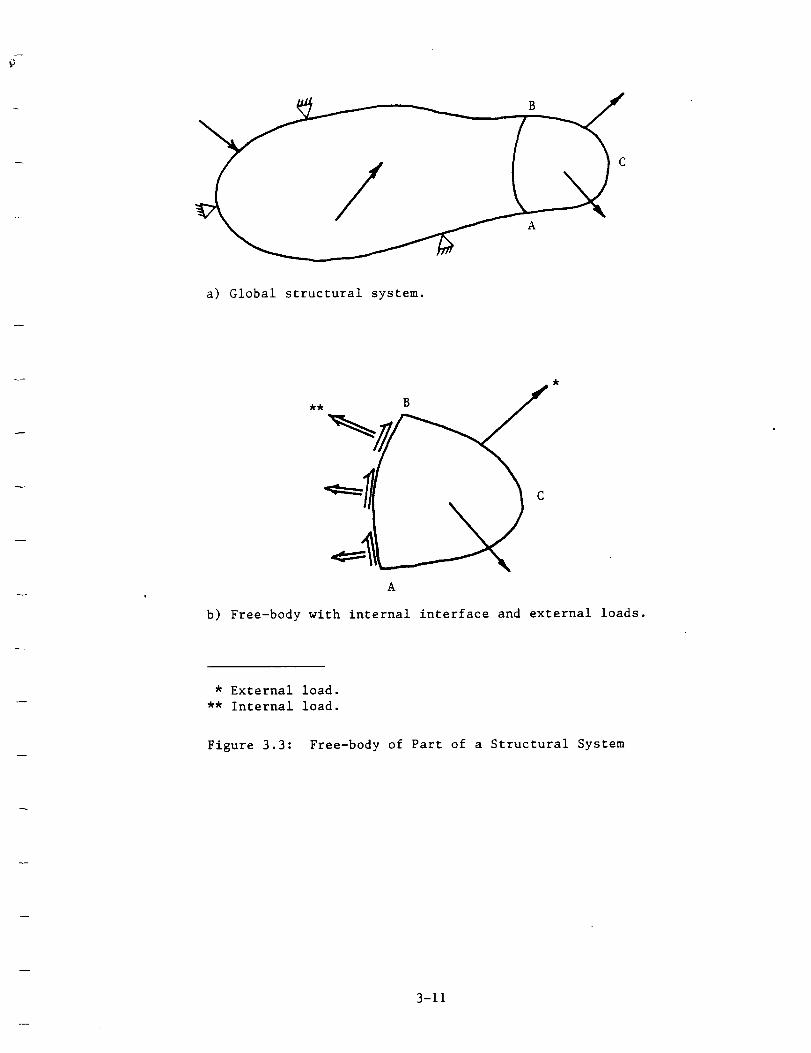
B
a) Global structural system.
A
b) Free-body with internal interface and external loads.
* External load.** Internal load.
Figure 3.3: Free-body of Part of a Structural System
3-11

The matrix equation for a free-body can be written as follows:
Nf_f + Cfqf * Kfqf = ff(t) (3-14)
where fff, Cf and Kf are the mass, damping and stiffness matrices for the
free-body, respectively, and qf(t) and ff(t) are the displacement and
applied load vectors for the free-body, respectively. The free-body is a
free-free structure--no displacements or rotations are prescribed on the
interface surfaces of the free-body, i.e., on Surface A-B in Figure 3.3.
The applled force ff term includes all forces applied to the free-body,
including the interface forces.
Given a free-body together with all applied loads, the solution to
Equation 3-14 will be the same as the part of the solution of the global
problem corresponding to the domain of the free-body.
The module (in this case, a free-body) transfer function matrix is
determined by Fourier transforming Equation 3-14. The following is found:
(-_aMf + it_Cf + Kf)Qf(e) = Ff(_)
or (3-15)
Thus,
KfQf(e) = Ff(e)
Qf(e) = KflFf(e)
and the transfer function matrix is seen to be Kf
tion occur when
(3-16)
The poles of the func-
Oet(Kf) = 0
which also corresponds to the eigenvalues of the free-free module.
3.2 Examples of the Module Transfer Function
Three examples of the module transfer function are presented. The
examples are simple (a few degree-of-freedom), but clearly illustrative of
the concept.
3-12

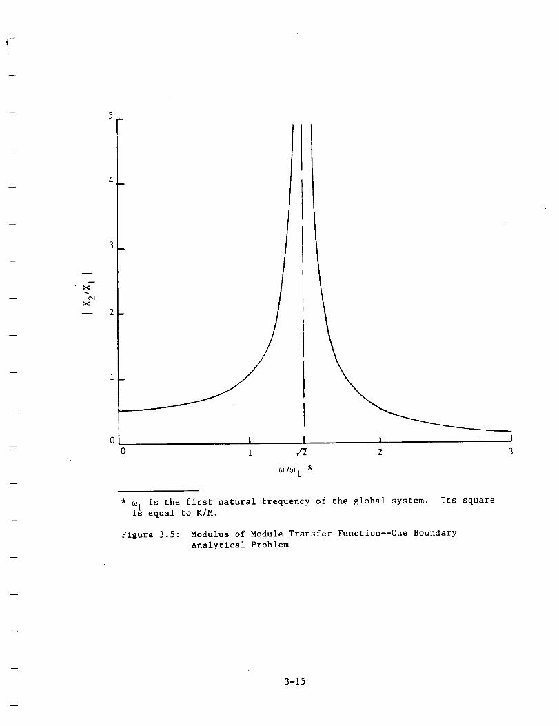
3.2.1 Module With One Boundary Point - Analytical Study
The module and global system studied is pictured in Figure 3.4. The
system is excited by a harmonic force at Node 1. The module transfer
function modulus for this case is
i 4-- IKii{={x2jx1{
where X1 and X 2 are the global structure responses--modulus of the steady-
state response. A plot of the function is given in Figure 3.5. There is
one pole (_P)2 = 2e_ = 2 K/M. The one natural frequency of the module with
the boundary fixed is seen to be equal to e p.
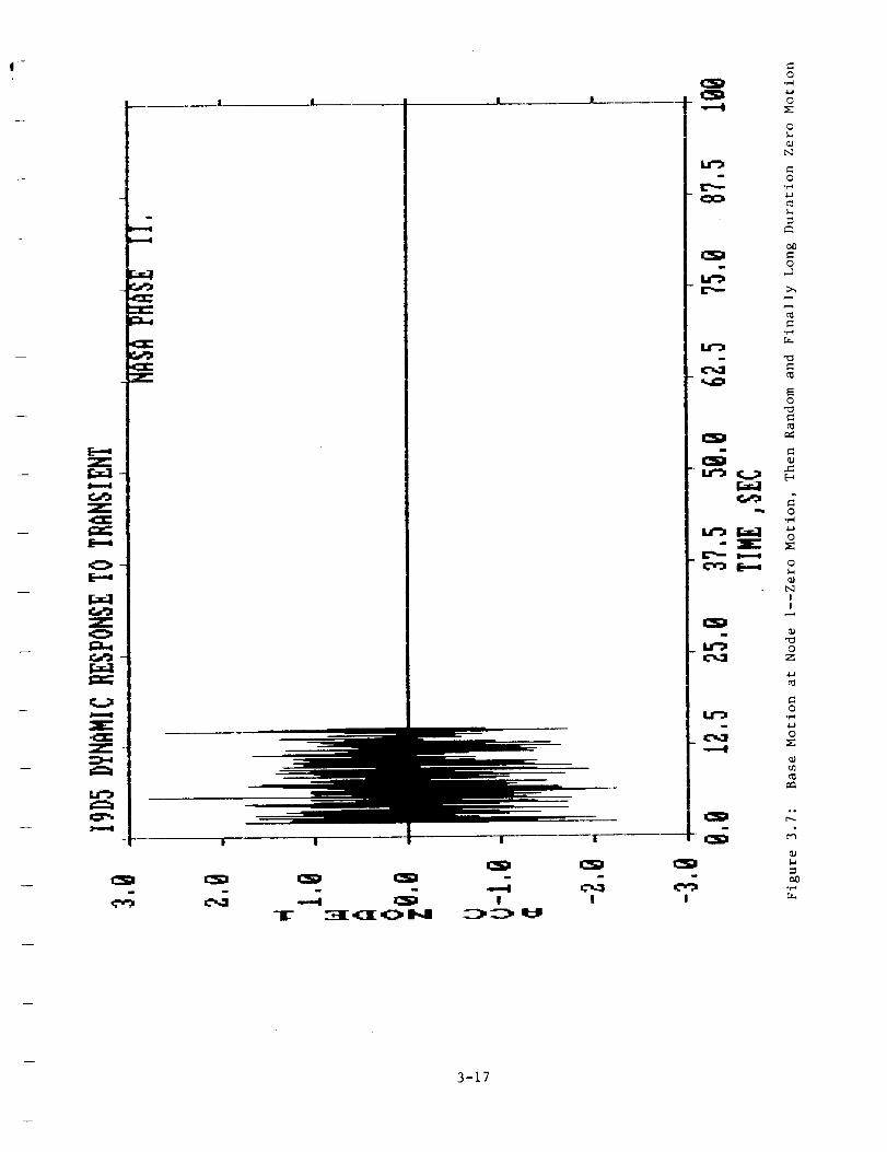
3.2.2 Substructure With One Boundary Point - Numerical Study
This numerical study involved a single substructure boundary point--a
single input to the substructure (there were no forces applied to the
substructure interior). For this study, several different locations for the
boundary were chosen (see Figure 3.6). For a given substructure, a transfer
function was calculated by dividing the Fourier transform of an output by
the Fourier transform of the boundary motion*. The response of the global
system was determined using the static and dynamic structural digital
computer code COSMOS/M. *s
A single approach was used to excite the global system--it was base
(at Node 1) motion. Figures 3.7 and 3.8 show a sample of the type of input
used and a sample of the outputs obtained, respectively. The first transfer
function obtained was for the global structure (see Figure 3.9). This was
done to verify that the correct method and parameters were being used to
obtain the transfer functions. Because of the nature of the excitation, not
all the modes were excited. A comparison was made between the poles of the
This was done using the digital computer code MAC/RAN IV [3]. This is a
proprietary code developed and marketed by University Software Systems,
El Segundo, California.
** A finite element code developed and marketed by Structural Research and
Analysis Corporation, Inc., Santa Monica, California.
3-13

F xl F x2
Flsin(_t)
J_- y
Module
Figure 3.4: Two Degree-of-Freedom Lumped Spring
and Mass System--Module With One
Boundary Point
3-14
m
¢q
x
4
! I I0 1 _ 2
co/_ 1 *
* e I is the first natural frequency of the global system. Its squareis equal to K/M.
Figure 3.5: Modulus of Module Transfer Functlon--One Boundary
Analytical Problem
3-15

x(1)
r _
i 2 3 4 5 6 7 8 9 i0
a) Global Structural System*
X
b) Module l--Boundary at Node 9
b(1) (i)X X.
i
r r
9 10
_ X
c) Module 2--Boundary at Node 8 _____x8 9 I0
di Module 3--Boundary at Node 6
x_,)x_,) x!4)1
___.x6 7 8 9 I0
* The masses move in only the x-Direction.
Figure 3.6: Nine Degree-of-Freedom Lumped Spring and Mass System--Various
Modules With Single Boundary Point
3-16
0
Z
-i
m
m
m
q.--I!
::_1, :Z_. 'I=11
! !
J
m
u
--,Jr
i
_ II,.I'_
I
0
0
0
©
0,-]
"0
0.-_
0
0
0
II
0Z
0
0
oo
I..i
0.0
3-17

I[..T-11-
0
I I
l I
,.,49
flail TT--
i IL
| |
= _ .---4! !
-.--I
0
_ *r-t
_ o-_,- _
-- 0
Q
°_...I
@
_ m
_ o_ m
1.1
0 0_ z
_ _._ o_ o
-,-4
a
!
3-18

r_ink.
Z
Z
0
r..T..I
Z0
Z
m
b,-
m
|
r
III_I TT--
m
nE_ "II:"
II |
b_ i
! !
m
m
e
u
!
0
0
Z
0
o
0
c_
_J
3-19

global transfer function and the natural frequencies obtained from an
elgenvalue extraction--there was excellent agreement between them. Also.
the damping obtained from the global transfer function was compared to that
used in the simulation--the comparison was excellent.
Transfer functions were then obtained for the modules defined in
Figure 3.6. They are shown in Figures 3.10 through 3.12. The results are
completely consistent with the theoretical results discussed in Section 3.1.
Table 3.1 Is a comparison between the poles of the selected transfer
function for the module and the real natural frequencies obtained from the
fixed boundary module elgenvalue problem. It should be noted that the
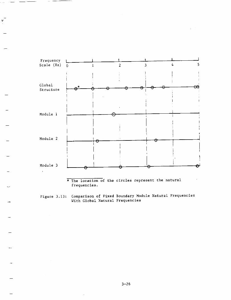
module poles are different from the global system natural frequencies (see
Figure 3.13).
The last thing to be discussed for the one boundary point module
-problem with base excitation is the effect of changes In the structural
system external to and at the boundary of the module on the module transfer
function. Theoretically the module transfer function should not be changed
by changes external to it and at the module boundary. It was decided to
look at this for the numerical example being studied. This was done by
reducing the mass at Nodes 2 through 6 and obtaining a transfer function for
Module 3. This was done for two levels of mass reduction--25_ and 50_
reduction s . The results are shown in Figure 3.14. The transfer function
(e.g., AIO/A6) remained virtually unchanged. The largest changes in the
modulus (magnitude) occurred at the first resonant peak (at 0.69 Hz). The
"peak frequency" remained unchanged, however, the amplitude at the peak
changed slightly. This is probably due to the fact that the module transfer
function peaks occur at frequencies which are between the global structure
frequencies; hence, the module transfer function peaks occurred at
frequencies where the input was quite small. Thus, numerical problems may
have caused the slight variation in the peak height of the first resonant
peak. The phase remained virtually unchanged for the three resonant peaks.
= These reductions in mass, 25_ and 50_, represented a 13.8_ and 27.5_
reduction in the total mass of the global system.
3-20

15,0
12,5
L9,8J
7,5
¢I
15,8
I
2,5
8,8 t
FREQ.,HZ
4! 'il
i "8,88 1,25 2,58
a) Modulus--Input is A1 and Output is AIO
8,8
-48,8.
-68,8-
_4
_-88,8-
-L88,8
NASAI9U; RESPONSETOTRAHSIEHTTRACE,d I i I
II
\\
b) Phase
Figure 3.9:
AtO/A,L(18000POINTS)HASAPHA_SElI,'
,.,L_.r_._.L •.:
, I, r
1',25 _.,58 3,75 5,89 B',25 7,58 8,75 19,FREQ,HZ
Global Transfer Function--Node i is the Base and Nodes 2
Through I0 are Other Structure Points
3-21--# -_,,r ,
OF I_C_ QU_;.::_"Y

NASAigu;RESPONSErOTHETRANSIEHTiRAtE,-_,J_ / _-_ ...........12,0 , N_SAPHASEII,
10,0
8,0
60,0_S_ lgU;RBP_SE;0THE_RAI_IDITT]]nCE,AIO/Ag(IO080 POINTS)
' ' ' ' H_S_PHA_EII ' '' I
'_ 40,0
20,0
O,O
-40,0.
-60,00,00
.r..-_
k"---""_-'- ...._-=_-_r_ JI
b) Phase
Figure 3.10:
1,25 2,50 3,75 5,00 6,25 7,50 8,75 I0,
FREq,HZ
Module Transfer Function--Node 9 is the Boundary andNode I0 is the Interior Point
3-22

15,@. NASAPHASEIT,
12,5 ._I
J
IQ,s1
7,5
2,5
@,@
u
ii/
i
@,@@
1 i
\ ^_"-----_/'_""--_--_'_'_r'-,_"--_:'-_---_
1,25 2,5@ 3,7S S,@@ 6,25 7,5@ 8,75 1@,FREQ,HZ
a) Modulus--Input is A8 and Output is AI0
6@,@NASAIOU;RESPOHSEIOTHEI_NSIENITRACE,AiO/AB(I@@@@POINTS)
' ' + ' NASAPHAS£IT,'
2@,@
_-2@,@
-4@,@
-6@,@@,@@
b) Phase
Figure 3.11:
I
r
\
P
J.,25 2,58 3,75 5,88 6,25 7,5@ 8,75 1@,FI_, HZ
Module Transfer Function--Node 8 is the Boundary andNodes 9 and I0 are Interior Points
3-23

t2,_NASAI9U; RESPONSETOTRAHSI_TIRACE,
, i
I
[
8,8 1
I
6,0 4
¢Z4,0
_,8
8,88,88 1,25 2,58 3,75 5,B@ 6,25
FREQ,HT,a) Modulus--Input is A6 and Output is At0
AtS/A6(18888POINTS>
NASA'PHASEII,
?,58 8,?5
8,8
-25,8
_-58,iiI,
-62,5
I_SI_19U;R£S_HSEfOT_NsIDrIf_Cl,i I i i '
_:o/A6(lorePOINTS)_sAP,ASE[:,' "
-75,8 , ,8,80 1,25 2,58 3,25 5,8@ 6,25 7,58 8,75
_Eq, HZb) Phase
18,
Figure 3.12: Module Transfer Function--Node 6 is the Boundary andNodes 7 Through I0 are Interior Points
3-24

TABLE 3.1: COMPARISON OF MODULE TRANSFER FUNCTION POLESAND MODEL NATURAL FREQUENCIES
Module
3
Observed Pole
(Hz)*
Natural Frequency
(Hz)**
1.78 1.78
1.13 1.15
3.40 3.38
O. 69 O. 70
1.99 2.01
2.99 3.09- 4.91
* The frequencies were obtained from the transfer function plots; thus,
there will be a small amount of error in the reported results. The
fourth frequency for Module 3 was not detected probably because of the
nature of the global system excitation.
** The natural frequencies were obtained from the fixed boundary module
eigenvalue problem.
3-25
Frequency I
Scale (Hz) 0
i I I ; J
1 2 3 4 5
Global
Structure
Module 1
Module 2
Module 3
vIT% I"% f2% @ G
(D
0
fI
o I 0 0
0
i
* The location of the circles represent the natural
frequencies.
Figure 3.13: Comparison of Fixed Boundary Module Natural Frequencies
With Global Natural Frequencies
3-26

3-27

T
!
!
.J• !• !i I
• i !
!
I
f--
.it
°_
C,,,)
_ ),,,a
m o _ >
m o
-M
T r r
! ! !
n
!
!
3-28

3.2.3 Module With One Boundary Point - Two-Degree-
of-Freedom System With A Local Mode
In the previous subsection (3.2.2), the module had a single boundary
point (one degree-of-freedom at the boundary). There was a slight error in
the module transfer function modulus for the 25_ and 50_ damage outside of
the module (reference Figure 3.14). It was decided to investigate this
problem further using a simpler lumped mass and spring system (see Figure
3.15). Further, the system was tuned so there were cases with only global
modes or a local mode whose motion was largely restricted to the physical
domain of the module.
The first case looked at is somewhat similar to the previous one -
the modes are global (see Figure 3.16) and there is a slight change in the
amplitude of the module transfer function modulus near its resonant peak for
damage outside the module (see Figure 3.17). For a 50_ increase in
stiffness outside of the module (resulting in a 15_ increase in the global
fundamental frequency), the indicated resonant peak for the module increased
in height by 7.5_. This result is not new.
The next case consisted of tuning the model so one of the global
system modes has its motion local to the module only--a local mode was
generated (see Figure 3.16). The structure was damaged outside of the
module in the same way as for the global case (50_ increase in stiffness).
However, because the first mode's motion was local to the module, the
fundamental global frequency essentially did not change--0.4615 Hz and
0.4698 Hz undamaged and damaged, respectively (a 1.8_ change). There was
virtually no change in the module transfer function modulus near it resonant
frequency (see Figure 3.16).
When a global mode's motion is "local to a given module", any
excitation external to the substructure will be transmitted to its boundary
fairly well unmodified within a narrow frequency band containing the modes
natural frequency. (It is assumed that the adjacent modes are not too close
in frequency.) This can be seen by looking at the local mode shape for this
example and the corresponding Fourier transform of the base excitation and
system response at Node 5 (see Figure 3.19). If the base excitation is
broad band white noise, the substructure boundary motion will be essentially
the same. Thus, it will be possible to determine the module transfer
3-29

!
rxl
K 1 M 1 K 2 M 2
M_:M2 ! J- Module -I
Case System Modes4
1 Global 1
2 Local/Global I/I0
Undamaged Stiffness
Ratio, K2/K 1
* There were nodes which were intermediate to the nodes shown.
They have not been shown here because the mass associated with
them was much less than M 1 or M 2.
Figure 3.15: Two Degree-of-Freedom System With and Without a Local Mode
3-30

I 1.6
Mode i
1.6 i
r
Mode 2
a) Case I - Global Modes
I I0
r
Mode 1
9.4 1
b) Case 2 - Local/Global Modes
Mode 2
Figure 3.16: Mode Shapes for Two Degree-of-Freedom Undamaged
System
3-31

31._
_.¢3_
0
E,.--,I
f.,,,t..1
.-j.-
_ E--,.,a
.-7-
u._
| ! J !
n.-.l
•'Ig ,_i
o m
r-( ,,_ .,-i
¢.i
_ _,._ •
m o •
_ c_ j:: cJ
(J o _J
• _ _ 0
• __
I | ! I
//
/
0
.-_
._1
J_
¢J
0
_J
n,
I
0 J:_o
I
°,r--.
=
3-32

I
i
,.--4
Z
C2_C_
V
l-i-I
Z
O
_r.T.1
O
--r
I I I
.'/.7
.C C
o
m o _u.c:
F _ _ C
m m •
t °u'3 "_
!dl ,.--I
l | |
-- _ ¢_II I I
i
-,.--II
o
v
N
_0
i
|
3-33

m
V
E
-- 0
0
Z
m
o ou_
-N
m
I
C
> _
_ >c m
I I I
m
!./
----.......__
m
" C
-M
C
r.
!o
r _, o_
u
o
t,M
c o
_ m
g;
¢¢3
3-34

! !
"0 cJ u_
,-4 0
.-M _0 .,'-_
_ _J _ °
_o
N
I !
_ -lg-
! !
i-
! !
I !-_-_ _ _ H_
I
I
"0
"03,-4_J
0_J
cO
r_
3-35

I
a o ':_.°_ ............
a a a a a ,-, a a a a a_...__-'-:_-
3-36

function within the frequency band with a good degree of accuracy. This
would be true for sine dwell excitation if the narrow frequency band was
"swept".
There appears to be somewhat of a problem in obtaining the module
transfer function when the structure outside of it modifies the excitation.
If the excitation to the global system is broad-band white noise the
structure changes it so the substructure boundary motion is not white noise
within frequency domains containing global modes. Thus, the corresponding
module transfer functions cannot be determined using external excitation.
Excitation from within a substructure will be investigated later in this
section.
3.2.4 Module With Two Boundary Points
The module to be discussed is pictured in Figure 3.20. There are
three springs (each with spring constant K) and two masses (each with mass
M) within. The structure outside the substructure is not defined yet.
various matrices needed to determine Kli are given as follows:
Kii = K1 EM03, Mii =- 2K O M
For this example, take
matrix is
The
= O; thus, a "complete" module transfer function
_--I _
-KiiKib
The matrix Kib is
3-37

K M K M K
X
Module
Figure 3.20: Module With Two Boundary Points
3-38

Because the global mass matrix is diagonal Kib = Kib. Thus.
JK(2K - _o2H) K2
~-1 ~ 1
-KiiKib - Det(Kii) K 2 K(2K _2M
where Det(Kii) : (K - _2M)(3K - _2M)
The 1,1 element of the transfer function matrix is represented by the plot
in Figure 3.21. The square of the transfer function poles are given by K/M
and 3K/M, which are equal to the fixed boundary module eigenvalues.
3.2.4.1 Numerical Example of Two Boundary Point Problem
The previously defined module with two boundary points was
incorporated into a system, with the total system containing nine lumped
spring and eight lumped masses (see Figure 3.22). The global system was
initially excited using base motion at Nodes 1 and 10--the motion was
random, equal for the two bases and in only the x-Direction. The transient
problem was solved using modal superposition. The global system responses
for Nodes 4 through 7 were saved and used for the module problem. The
global responses at Nodes 4 and 7 were taken as the inputs to the
substructure--the boundary motions. The substructure responses were taken
as the motion at Nodes 5 and 6. Table 3.2 is a listing of the undamaged
global system and fixed-boundary module natural frequencies.
The transfer function matrix (a 2 x 2 matrix) corresponding to this
module was obtained using ANCO's macro MIHO; the macro solves the multi-
input multi-output transfer function problem _. Figures 3.23 and 3.24 are
plots of the modulus for two of the elements of the transfer function matrix
(Appendix C contains all the plots corresponding to this matrix). The plots
correspond to a system state defined as undamaged and two damaged states.
* The macro MIMO uses the computer code MAC/RAN IV to solve the multi-input
single output transfer function problem for a linear system. Appendix B
briefly discusses the theoretical bases used for these computations in
MAC/RAN IV.
3-39

m
3O
2
'I
0
0
* w_ is the first natural frequency of the substructure with
fixed boundary.
Figure 3.21: Modulus of Module Transfer Function Matrix (Two Boundary
Point Structure)--Element i,I
3-40
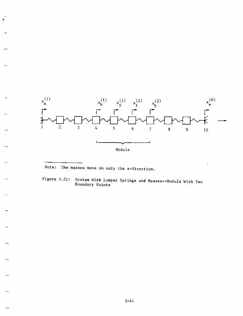
x (I) x(1) (2) (2)e x_ I) I" xi xb x(6)e
C r r c r c
1 2 3 4 5 6 7 8 9 I0
Y
Module
Note: The masses move in only the x-Directlon.
Figure 3.22: System With Lumped Springs and Masses--Module With Two
Boundary Points
3-41

TABLE3.2: UNDAMAGEDGLOBAL SYSTEM AND MODULE (FIXED-BOUNDARY)
NATURAL FREQUENCIES
Mode
Natural Frequency (Hz)
Global
System Module
0.746
1.407
2.226
2.594
3.159
3.675
4.865
4.956
2.460
4.753
3-42

a) Undamaged System (Initial Configuration)
i
\15,t-
b,°!i
5,0.F
IF_!Fii__N 2lm__ - Irmll¢m mz,i
il
/
' I
ti
' I1 r
0, 0 i
u _,o to _,o 4,o _,o 6,0 7,o s,orile
b) System Damaged Outside of Module--
Fundamental Global Natural Frequency
Changed By -23.5%
nail !11! lu! W- lille
6,o I .... _ m mx,u
1,| <1\
qi
i,o_tF
W
r i '_ ;
i '
/ i
i
t,o _.o i,o 4,o _,o _,o 7,o to
c) System Damaged Outside of Module--
Fundamental Global Natural Frequency
Changed By 23.3%
IlAI1 II l II t II • lii¢.... / I ll,i
II
1.I I,I I,I II f,I _t 1,1 LItl
Figure 3.23: Comparison of MIMO Transfer Function Moduli for J8
Model; Element Output 5, Input 4
3-43 OF PO( _ QUAL_i*Y

a) Undamaged System (Initial Configuration) 101a
'l_,o!
1111111Jll)IIIU - IIIIII(
.... wunr_u'mum'mx.iI
e0,Oi
i! 'i
, I0,0 i .
o.o L,0 2.0 3,0 t0 S,0 _.0 7,0 1,0FIB,IR
b) System Damaged Outside of Module--
Fundamental Global Natural Frequency
Changed By -23.5%
z0)n I
' iI
I
t"i.[
mHll IIII|II- IIB¢
.... _ m _li,i
kl I,! I.I 1,I ¢! _I £! 1,0 Ll1111
c) System Damaged Outside of Module--
Fundamental Global Natural Frequency
Changed By 23.3%
lll1111lI.llIIIIII -llll(
i,o) ' _ B _).,I
t! -'
Figure 3.24:
i
(,0_ !
t 'III,Ii _ ,', i
[
,,i
LO _. ....0,O ].I _,O 1,0 tO _.O 6.O 7,0 8.0
I|
Comparison of MIMO Transfer Function Moduli for J8 Model;
Element Output 5, Input 7
3-44

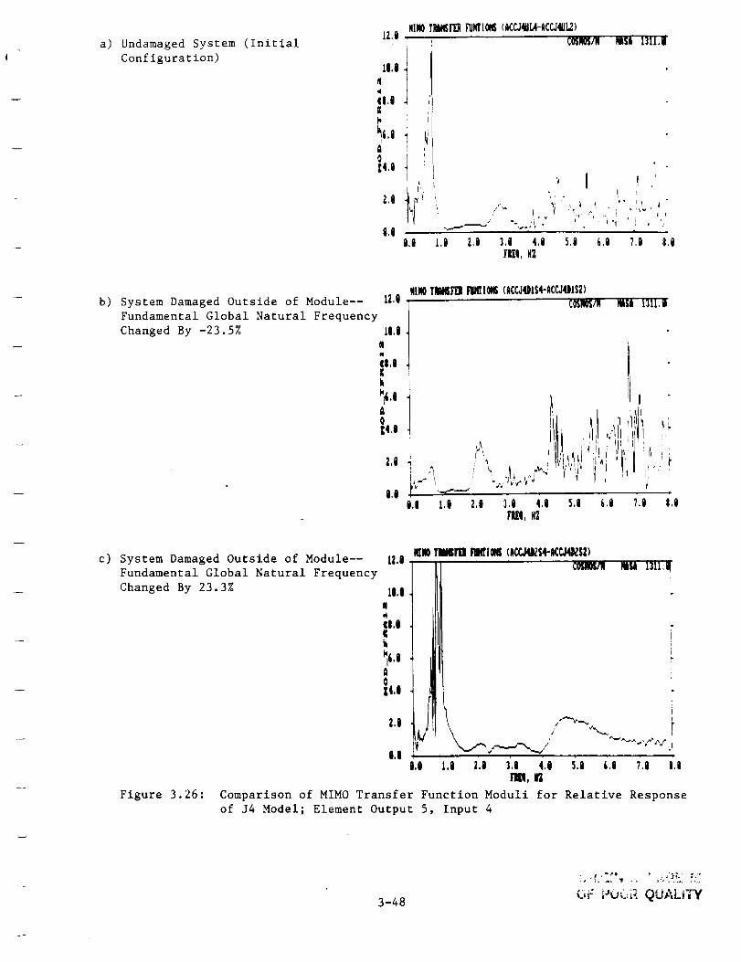
The damage corresponds to changes being made to the global structure outside
of the module. Thus, no changes were made to the module transfer function.
However, the module transfer functions computed for different damage levels
clearly were different. The "transfer functions" computed are not the
desired functlons--these are not transfer functions, they are merely
functions of frequency which are dependent on the global structure
properties.
Why was this result obtained? The procedure used to obtain the
module transfer function is based on the current technology used to solve
the multi-input multi-output transfer function problem. One major
assumption used in developing this theory is that all the inputs to the
linear system are independent of each other. This is certainly not the case
for this or related problems--the inputs (boundary motions) to the module
are dependent on each other because they are responses of the global system.
Because of this and what is to be presented, it will be shown that
determining the module transfer function matrix is very difficult and
probably not possible for a completely general case.
The transfer function computations described above used absolute
module responses. It was decided to perform the same computations except
using relative module responses. Instead of computing .the relative
responses by the pseudostatic method described earlier, they were obtained
by defining a separate free-free structure and including only those mass
degrees-of-freedom which corresponded to the global system module (see
Figure 3.25). Large masses were assigned to those degrees-of-freedom
corresponding to the module boundary points. Then, forces equal the large
masses times the corresponding module boundary accelerations were applied to
the large masses. The resulting absolute motions of the free-free system
matched well with those of the corresponding global degrees-of-freedom.
This approach to the enforced motion problem is discused in Appendix D. The
relative response of the module was then obtained by using only the third
and fourth modes of the free-free system in obtaining the solution to the
transient response problem s .
* The first two modes were rigid body and near rigid body (very low
frequency) modes, whereas the third and fourth modes were essentially
fixed base modes--Nodes 4 and 7 were virtually fixed.
3-45

x 4 x 5 x 6 x 7
F r r r .
f4 _ f7
Figure 3.25: Free-Free System, J4, Used to Determine Relative
Response of J8 System
3-46

The 2 x 2 module transfer function matrix for relative module
responses was then calculated (see Figures 3.2G and 3.27 and Appendix C).
Problems similar to those for the absolute module responses are evident here
also--the transfer function changed with damage outside of the module. The
transfer function poles corresponded to global, as well as module, natural
frequencies. No additional insight was gained by looking at the single-input
single-output (SISO) relative transfer functions (see Figures 3.28 and 3.29).
The global resonances were clearly evident. The only thing that was an
improvement was that there was no evidence of the fundamental global natural
frequency--using relative responses eliminated the peak corresponding to the
fundamental global frequency.
It was tentatively concluded that the module transfer function
matrix for the case of multiple boundary points and excitation outside of
the module could not be calculated by the approach used and described
herein. This is true for absolute or relative module responses. It was
decided to see if exciting the global system by applying a force(s) within
the module would help in the determination of the module transfer function.
The general idea is that if the forcing within the module can be chosen such
that the response of the module is due largely to it and only slightly to
the boundary motion, possibly the problem may be reduced largely to a SISO
transfer function calculation. This can be seen by looking at Equation
3-11. If
> > 2 -1F i w MitKiiKibXb
within a given frequency domain, then within this domain
KilR i :' Fi
and the module transfer function matrix can be easily calculated using
the MIMO procedure described herein.
This was done for the subject numerical example using relative mod-
ule responses. A force, fs(t), was applied to Node 5 of the global system.
The previously described procedure for determining module relative responses
was followed--for the J4 model (see Figure 3.25) the masses at Nodes 4 and 7
were driven to obtain motions equal to the corresponding ones of the global
system and the force f5 was applied to Node 5. As before, this produced
3-47
a) UndamagedSystem (InitialConfiguration)
121
ll.I
c|,l
I,
!LI
i.i
Mill) tll_lrD _lOgS (_CCJeiUI-_C_eI2)COSM/R
1 L
'1I
I,I
,i
i
m J
L.O 2,O 3,i q.I 5.0 6,0 7.0 8.1FIIi|, N_
b) System Damaged Outside of Module--
Fundamental Global Natural Frequency
Changed By -23.5%
ILl
li,I_t
¢1,0lk
_li.|
Z,i
i,i
lllll 'lliii11] I'III_I011(I¢C51111S4-ilCCJ411$2)'C0$11Klg NI$1' ].31L,i
j
I Ii ,_!I_,,,illi ,_Ibl_,:!il_!I i
,, _!_,_,I_i'_!'_i__l,i_,,',,,'i ';'v" '_"' ' P ¢ 't
i
I.I l,I 2,1 3'.1 q.I 5.1 ;,i ?.i $,gfilL1, N2
c) System Damaged Outside of Module--
Fundamental Global Natural Frequency
Changed By 23.3%
Figure 3.26:
LLi
_ILI'I
l,i
_I.II
l,I
I,i
lllll0 'lllgllrD IriRlOgl (t¢O_I¢OOZSl)
111\ ,"'_o_ _
e,e _.,e :,,e _',e 4,e S., _.e '_,e e,e1111,I_
Comparison of MIMO Transfer Function Moduli for Relative Response
of J4 Model; Element Output 5, Input 4
3-48
r
_,F i-'u_(_,i_ QUALITY

a) Undamaged System (Initial
Configuration)
I
i
b) System Damaged Outside of Module--
Fundamental Global Natural Frequency
Changed B -23.5%
HIMTRIIIISFI:IIFIIIITIOMS(l£_J4DIS4-A_Y..JOI$2)12,0 COSIO0_ MIISIL3LI.I
lll.lel
II,Il
1
Z,i
0,0_.+- _,. ++ ,#
O.O l,I) Z,I)
i
i
I i/
I|_I _i ",_ ii :"i ,_; ' t _/ ' 'i I _
• I
3,0 4.0 5,0 6,0 '7,0 8.0FP_, NZ
c) System Damaged Outside of Module--
Fundamental Global Natural Frequency
Changed By 23.3%
il.l
ll.llfII,IIk
1
l.I
I,I
IIM Tiilrll illMlOll (_]4]_54-1_,J4J_2).... _:_,
I1.1
ms,i
P
I
l.l l,l 3.0 4,1 5,1 i,l 7.1 l,OFILl,113
Figure 3.27: Comparison of MIMO Transfer Function Moduli for Relative Response
of J4 Model; Element Output 5, Input 7
_+# +'++_..:+. i L/:.:rAj.i-,,y 3-49

a) UndamagedSystem (InitialConfiguration)
L2,N,
il.N]
I,N J
LN
Z
O,Nt,I l,i 2,0
_A"J+U _ - _''_4 J! "COSHOs/]qMSli' L]ll,iltLr'lrOF RIIA¢_
HI?'II AI_ACC!D O,[r, :BAHI_IDi'It: 3,296[-i_!VAILIKr : 2.|71|-_I
: 2.267|'01_.
/
3,0 4,1 50 +,+ 7,0 8,_rP,_i_cY
b) System Damaged Outside of Module--
Fundamental Global Natural Frequency
Damaged By -23.5%
L2,8
ll,l
I,I
6,1Z
Z,O
i
0.00,0
"t "" '++' 'S u+-- _'+'J: :'_"COSPlOS/NNASA'I)II,Ul'lrr OF P_A¢_
H[TN AKACCLD,O,Lr, : J,,.hI_IIDTN : ),2761"12_
: l,g$6l'Ol,.
_r _
L,i _-',i 3,0 4.0 5.0 6,0 ?.O 8,0rl_[1_t "
c) System Damaged Outside of Module-- LL|
Fundamental Global Natural Frequency
Changed By 23.3% LI,|
I,I
LI
ZN
¢4,1l,l
Z,I
i.|
f A:':J4 _ 15_ - ,a,',+-r,_C2_q2")
Ml_llTll'O'r': l,|_['_Vllltl_ i,1361"11
1,l?l'll_t
i,I
f-_,/
/ _ i
t,O _.0 _'.0 _,0 _,0 +.0 _,| _.e
Figure 3.28: Comparison of SISO Transfer Function Moduli for Relative
Response of J4 Model; Element Output 5, Input 4
3-50

a) UndamagedSystem (InitialConfiguration)
I2,M
ll,B.
I,N
&,N i
Z i
_4,01
0.0
cosm/W Msi t3u,a
AiS_¢4D,O,F, : ¢milDtH : 3,27||'i1_]UllillKr : 2.l?l|-i_I
: Z,ll+t-at+
I+ .,
l,ii 2,i 3',11 4,0 5,6 &,0 ?,0 8,8I'RlmUD4PI
b) System Damaged Outside of Module--
Fundamental Global Natural Frequency
Damaged By -23.5%
12.1
ll,l
l,l
ill
Z
_4,0
Z,O
I,OI.I
"/4 '," 74TI_4- A+'_'74 _, IS2 )
_:mllO_ MllSll't3tt,_t_ O_ PlUCC2HITI tlISl¢C4 I
|,O,P, : 4i"ll_mlDi'll : 3,Z?61:-IgUIIIIIiC[ 3,Z?SE-131
3,S?&[-_
t"t
+
++I
_.j_"J !
PLPII_
c) System Damaged Outside of Module--
Fundamental Global Natural Frequency
Changed By 23.3%
lZ,I
ILl
I,I
&,l
Zm
¢4,IO
2,1
I,III,II
/ A,":'.74 _,254 - 4",++7_C'2S2 )i i
D_l_ IBK¢4 i
+IIIMIC][ : 6.131-iI_|l.+l+l-il!
Jt,o z,o 3*.o +.o
rmH_
/
i
\. ,_m_m._mw_ _
_r I _* O 1 , I I ' I
Figure 3.29: Comparison of SISO Transfer Function Moduli for Relative
Response of J4 Model; Element Output 5, Input 7
3-51

motions which matched well those of the global J8 system. Nodes three and
four were used to obtain the relative responses. Figures 3.30 (time
histories) and 3.31 (Fourier transforms) present the absolute boundary
motions and relative responses of the module. It is seen that the relative
r, rise of Node 5 is considerably greater than the absolute motion of Nodes
4 and ? (boundary points) in the frequency domain 4 Hz to 5 Hz. If the
motions of the boundary points within this domain was somewhat lower, the
problem would almost be a fixed-boundary problem with a single input (the
force at Node 5). This would indeed be a simple problem within this fre-
quency domain.
At this point it is worth looking at the difference between the
absolute and relative (as calculated) module responses for this problem (see
Figures 3.32 and 3.33). The major difference is that the relative responses
do not have a peak corresponding to the fundamental global natural
frequency, whereas the absolute responses do. There are other differences,
but they appear to be minor.
The 2 x 3 relative module transfer function matrix was then calcu-
lated (see Figure 3.34 and Appendix C). There is evidence of global motion
effecttng the calculated module transfer function matrix. The results are
poor; it was hoped that they would be better because of the excitation being
a force at Node Point 5. Some basic work/research needs to be done dealing
with this kind of NINO problem--the problem with dependent inputs.
One last thing will be discussed concerning this problem. For the
global excitation consisting of a single force applied to Node 5, it is
useful to determine how much of the module relative response is due to the
force at Node 5 and how much is due to the boundary motion. Ftg_are 3.35
shows plots of the Fourier transform of the relative response of Node 5 for
various applied loading conditions. Because the problem is linear the net
response (response due to the boundary motions and applied force at Node 5
acting simultaneously) is equal to the sum of the response due to the
boundary motions and applied load acting separately. It is seen that the
majority of the response within the frequency domain 4 Hz to 5 Hz is due to
the force on Node 5. This is good because when the J4 system (see Figure
3.25) is excited only by force f5, the masses at Node Points 4 and 7, M s , do
3-52

3,8
2,1
L,I¢
_8,o!II¢-LI
-2,1
REL./ABS.ACC.FI_-FO_R,J4F45?UACC(41q.-2N.),I_', F6-@_x-F'rr, j4F457u_'_(W
._ll_,ui J',-.ml I_d, llilL..IL_l ,h. ,.A_LAJil LJ.
-3,8 lo,, 3,, 6,a 9o i2,o Ls,o _8,a2t,o
TIME,SEC,
a) Absolute acceleration of module boundary
point at Node 4.
I
L1
4
Ir
[!L
q
24,
3,1
2.1
L,i
iI-I,II
-2,11
-3,11
IIII,/AU,ACC,FII-F(Hlll, J(AS?UACC(4M,-2M,),liT, FG:I' ' Rf_lN-f_, JCfq_Tg_F611
t
L
TL_, $(C,
b) Relative acceleration of module internal
point at Node 5.
Figure 3.30: Time History Motion of Module With Force Applied toNode 5
3-53

R_,/ABS,ACC,FIrP-FO_R,J4F157UACC(4W,-2W.),_, }6:G
3,8 _ ItF0UlI-ITT,J41r457Ull[6{
Li
¢J
l'l,g 4
i
-?.,i!i
-3,1 l
I.O
+i'ill" 'l'f'l ,'I ,"","_+v,t""+ """ "'_i,""
3,i 6,i 9'.8 12,i 15,1 18.8 31,Illill, SiC,
c) Relative acceleration of module internal
point at Node 6.
i
24,
llfI,tlIBS,tCC,tTT-FOUll,J4F457UACCt411.-,.II,,,liT, F6:i3.i , , , . RFOilll'II'i'I', J4F457O_[F61
2,1
l,i
iI-l.i ._
-_-,i 1
tI
-3,118,O
../IA*llAA.i_.ak. *__-i_+li..al._a_ __.._.. u.. --
3,i 6,i 9'.'8 i2,t i5.1 lit.ti 2i.il 24.Till, SIC,
d) Absolute acceleration of module boundary
point at Node 7.
Figure 3.30 (continued)
3-54

t50,8 _REL'SINP,TP_NS,FUNCT,-PSl),J4F45?URCCI4NODES-;'MODES),COSMOS/N"_S_ 131i,_
Iu,Qt I I
i!l! , ,
I I
-15Q,_Q,Q 3,0 6,0 9r,_ i2,_
IIMIo S_C,
I5,g 18,Q 21,8 24.
e) Force applied at Node 5.
Figure 3.30 (concluded)
3-55

24,8
is. 2t,i 116,1
_12,0 iV b
c i
BF.L./AB_,ACC.F_-FOUR,J4F4S?URCC¢4_.-2N.>,RT,Fb=Q
' " RFOOR-m,J4F157URIg_i
f
, _i . , ', ,!;"J'_'l
I,I I _' _'____+_-._"_.'" ..,,.'r r. '."; ' ', ' ""i,i 1,1 _.,t 3,0 4,1 5,1 6,t ?,i 8,0
fill, Iii
a) Absolute acceleration of module boundary
point at Node 4.
Jl lO,O,,i
llil,.lillS.llCC.ltlti-FOllll,J@45711llCC(il,-211.),l_, F6:i_4,1 ' .... _r_-il_, J41457U_T_6i
16,i
I1
ll,Ii
_s,i !11 l
4,1
Ii
s,i !I,I
i
I,l,I
t I II I] i#-' _ I
,'_1, "_ lily _1 I I
, ..-, 4w _, /,! i +
1,t _-,i 3,1 4,tFill, ill
I
5,0 6,1 7,0 I,I
b) Relative acceleration of module internal
point at Node 5.
Figure 3o31: Fourier Transform Moduli of Module Motion With
Force Applied at Node 5
3-56
R_,/A_.ACC.FFT-FOUR,J4F45"/UAO_i,_I.-2H.>,RT,F6:8
_-4,{, RI_OOII-{T'I',JO4571I_F6_-
'{211,11
I{,i
c) Relative acceleration of module internal
point at Node 6.
24,1
'02O,I
I¢,I
r,,cJIZ,I
¢
1
4,1
1.0
RD,./IIB._CC,iTt-F0Uil,J_45?UtKC(41I.-ZlI.),RT, FS:li
..... RlrOOl-lrPt', J4{'W_TtlXl{'5_
I.I t.i 2.1 3.6 4.1 5.8 i,I 7r'o
IPRL'{,H2
d) Absolute acceleration of module boundary
point at Node 7.
8,0
Figure 3.31 (concluded)
3-57

ABS,_CC,FrT-F_R, Je"45'Tt14ACC_4_ODES)24,0
.I
L6,tl
/I_12,1U
_1,8
1
4,1
8,0
AFt'm, J4F45'TU4:
Iq
i , I1!_I
{,8 1,8 2,8 3.8 4,8
F_Q, H2
I'+
li_ IIi
,' ;{ '1, _{ i,
i, : ,,',,/t5.o 6,o 7_ s,o
a) Absolute acceleration of Node 5.
i|
z4,{ I ..... _on-m; j_Tun_F_
2i,I "
li,I
flUI2.iU¢
8,1I
4,0
O.i
_I_,.'._.",t_'__{
l,l l,l _-,l 3,{i 4,0
Ili.._/,ii.i_,,,. ,, ,.I ;
5,0 6,8 7,e 8.0
b) Relative acceleration of Node 5.
Figure 3.32: Difference Between Absolute and Relative Module
Response--Fourler Transform
3-58
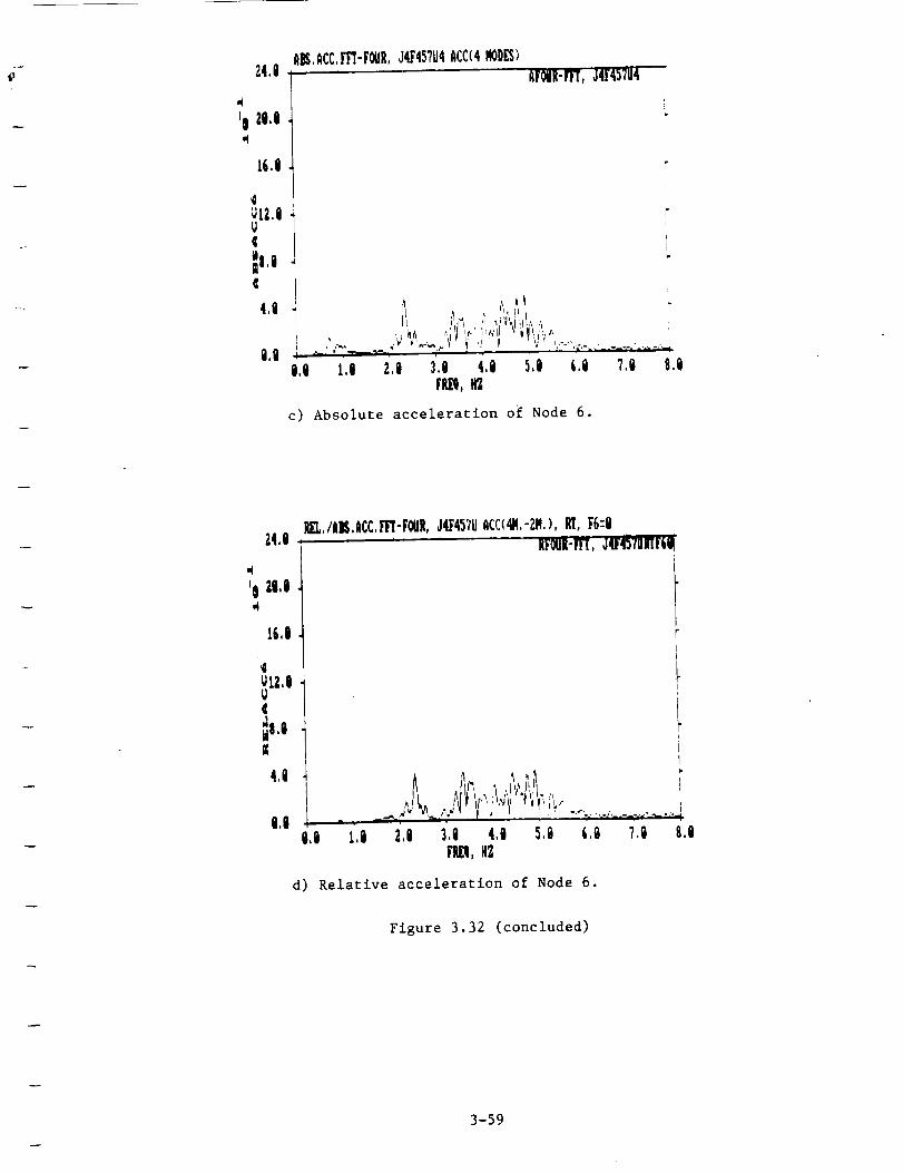
{E.ACC,m-FOUR,J4F45?H4_CC(4MO_[S)34.8 ,
,4
*l2i,I
16.1
AFOUR-m,J4F457U4
J]I
c) Absolute acceleration of Node 6.
_,aws.mcc.m-FOel, J4F45'zUACC(_.-2M.), {_, F&=O
Z4.i ....... RFOUi-{TT,JU4_TU{T_W
,W
'02i.iW
li,i
[2,1¢
Z
4,Q
i,i l',t_ i_ ,,..,_,,!,,_..,11,.., ............_
2.i 3.i 4,i 5.i 6.1 7,1 8.1
{11%KZ
d) Relative acceleration of Node 6.
Figure 3.32 (concluded)
3-59

6,1
_,5,1
4,,
L
¢ ,!
1,0
O,l)
SIMP_TI_I,_F_ PuI_rlOII- J4F45?U4(4NObk_, hBSASX/FOK_
I
I
I
-- L¢" ".%.
/ " 1
%.• i
, %%°.° _
/
/ I
._ "°.. L
i _ f',., /, b • }" I
FP.i:q,112
a) Absolute acceleration of Node 5.
i,l
N
l, 5,1.I
4.1
D
3.1i\
_2.tii
t,I
I.I
RI_./ADS._C.FFr-FO6R,J4F45?UACC<4Pl,-2H.),RT,F6"l.... +Ogll-_, TFJ+4_TUllTi611
+,'
. '_
.' % !
"=.o
t
+.."
,., I., 2., 3., +.o 5., +,, ?.,F1_, H2
b) Relative acceleration of Node 5
I'
ir
8,0
Figure 3.33: Difference Between Absolute and Relative Module
Response--SISO Transfer Function
3-60

i &,8
_| 5.8
4,8
_3,0¢I
_t2.{
F,
L.{
{.0
SI_I_T{_f{_ _N_f{O¢4- J4F457H4(4NOD{S),_BSA6X/FORC{15
' ' SIWErf_, J_W57U4
r
I
F
I
.,,. ..---'-" "--. i'+° %" ' _ 1• %
0.i t.{ Z.I 3+,0 4.0 5,0 6,0 ?,0 8.0FR_,N_
c) Absolute acceleration of Node 6.
&,i
Il 5.i,W
4,1
3,i\
l,I
I.I
P_,/AKACC,m-FOW{R,J4{'45?U¢¢¢(4W,-2fl,),RT, F6:O' ' ' _O({N-{TI'I'FJ4F4bTURTFG|
)
• _'\ ',.
o.o t.o z,o 3,o 4.0 5,o +.o ?.o o.oFro0 H_
d) Relative acceleration of Node 6.
Figure 3.33 (concluded)
3-61

M]_ R_,ACCk%,TRAMS,_H.-tRAMS,Jg4STUACC(AM,-2M.),RT, F'6--O
i lIi),O
3,o k
" I1 ]L'. -. +
o,o_,o _.o 2o
tli "+@" i
I
./
f" i++ i
+,,."/
I
)
L
+
3,o i,o i.o i,e 7,o 8,o[N_, H_
a) Element corresponding to output at Node 5,
input from Node 4.
lqIHOR[I,,ACCI_.TIiA_.FIIH.-I'RA_,J4F457UACC(4M.-2M.),liT,[(,:02.1,0 , .....
d
2g.ai
I
L
z i
0,0 +0,0
HASA"I31I,l
i
I
i11
_ A,_
I,I :_,1 3,1 4,1 5,1 i,I[qlZl, H2
"/,ll
!
8,0
b) Element corresponding to output at Node 5,
input from Force at Node 5.
Figure 3.34: MIMO Relative Module Transfer Function Moduli
3-62
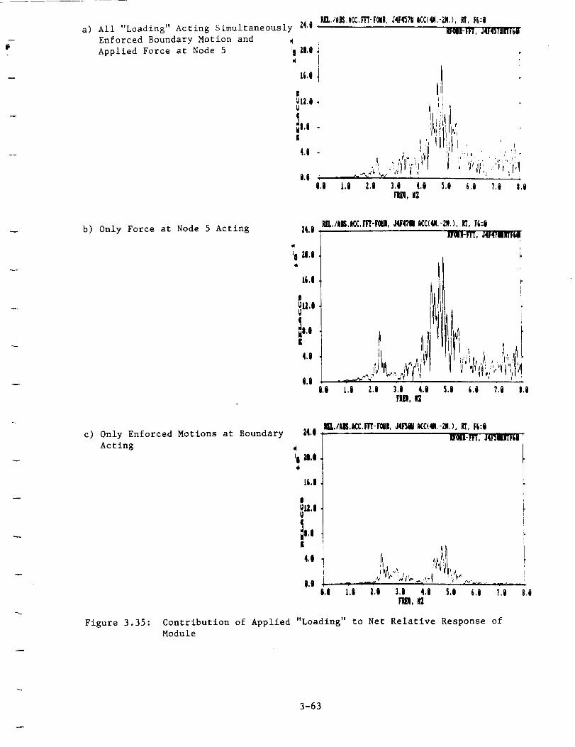
a) All "Loading" Acting Simultaneously 24,1_,/AII,ACCm-F0_R,J_45711ACCI_,-_,),,liT,F6:0UOOl'flrT, J_4_7JBffFGW
II il.l
I
12,0¢
_l,il
Enforced Boundary Motion and
4,1
Applied Force at Node 5
, ' t, j '' !P
+I ' '++r+++++ii ++++"- . _'_ -_ -v , l
1,1 2,1 3,1 4,i 5,i 6.i ?,i 8.iPLq, MZ
b) Only Force at Node 5 Acting 24,8 .I_./IIK.K¢,ITI-IIII, JqCffll I¢C(qt1.-211.),I_, fi:i..... iBwil-lTr, +q47111rlfil
+I 21.1,+
ti.l
I
_lJ.l¢
_I.I|
4,1
i
It/ I+il, !
L,I 2.1 3,1 43 5.1 i.i ?,l I.It1II, N2
c) Only Enforced Motions at BoundaryActing
,_.om'/','m m-m,.+ram_+_.-+,,+,_, +,-o' nm-rrt, J_.nr+u I
I1 21,Ig+
ti.l
I
i
¢
_l.iK
q,!
i.I 2,| 3,0 4,1 5,0 6,0 7.0 8,0F3L_ot_
Figure 3.35: Contribution of Applied "Loading" to Net Relative Response ofModule
3-63

not move and the solution to the problem corresponds to a fixed-base problem
with random excitation--the true module transfer function can be obtained
from this SISO data. A SISO relative module transfer function using the
force f5 as input was obtained for the case of all inputs to the module
acting simultaneously and only force f5 acting (see Figure 3.36). It is
seen that around 5 Hz they are similar and above 5 Hz they are almost
identical. This is an expected result. However, the SISO module transfer
function corresponding to all inputs is In error around 5 Hz and cannot be
used to represent the modules true transfer function.
What Is suggested by the above is a non-robust method for obtaining
a module transfer function. It deals with the selection of applied force
locations/directions (force appropriation). The approach is to apply a set
of forces to the global system, with at least one force being applied within
the module. They are applied in such a way that the module boundary motion
is zero within a frequency domain of interest. Then, within this domain the
module transfer function problem becomes a fixed boundary problem and the
transfer function can be determined easily. As the global system is damaged
{anywhere within the structure) the force Iocatlons/directlons must be pre-
served within the module, but may have to be changed outside of the module
so as to have no boundary motion within the frequency domain of interest.
This is not a very practical method of determining a module transfer
function, it is still best to try to develop a method of solving the MIMO
transfer function problem with some dependent inputs.
Another but very limiting approach to solving the module transfer
function problem is to focus only on those frequency domains where the
corresponding modal motion Is due to only global modes whose motion is local
to the module in que6tion. Of course, for this case the problem again
becomes a flxed-boundary problem within the specified frequency domains.
There are some good and bad points to this approach. The good points are
obvious. The bad points include: 1) there may not be the kind of frequency
domain described above--the global and global/local modes may be well mixed
together and closely spaced, and 2) there is a considerable amount of effort
involved in determining if the motion within a frequency domain is due to
only a global/local mode.
3-64

I &i
N
_{5,1
4,1
_3,0
\
_2,8
L,g
8.Jelo 3,+ 4,oFW, N2
_,/ASS,ACC,m-FOUR,J4F457uacc_,-2N,),_, F6:o
1
{
-' '.. i
+-+°
-..
E
:
r'_ • . . , L
l,i 2,0 5,0 _,t 7,8 8,0
a) All inputs acting simultaneously--enforced
boundary motion and applied force at Node 5.
6,1
_O5.0,,I
4,1
3,8\
REZ,,/ABS,ACC,PTt-F_N, J_4?OUACC(W,-ZW,),_, F6-O
/
i'
/
p
/
/
r
LI _"
i,I .._]/" k ._./'
o.o L,e 2.o 3,o i.a S.oFI_, N2
b) Only force at Node 5 acting.
I
I
', i
_,8 7,_
I
8,{
Figure 3.36: Comparison of SISO Relative Module Transfer Function for
Different Inputs Acting
3-65

6,8
L| 5,8
4,8
L,8
0,8
REL,/ABS,ACC,m-FOUR,J4F457tmACC(4M,-2M,),RT,B:8' ' ' _-FI_ TFJ4F457U_F6U
.e
Symbol Input:
All
Force at Node 5
c) Overlay of subfigures a) and b).
Figure 3.36 (concluded)
3-66

3.2.4.2 Module Transfer Function Via Time
Domain System Identification
Another approach to determining the module transfer function matrix
is by determining the module modal properties by using time or frequency
domain system identification techniques. Once the modal properties have
been determined the module transfer function can be determined. A basic
approach to this problem ls to use the matrix equation of motion for a mod-
ule for absolute or relative module response, i.e., Equation 3-13 for rela-
tive response in the time domain. Use the corresponding linear
transformation between the physical and modal domain to transform the equa-
tion of motion into the modal domain. Define an objective function which
expresses the difference between the model and experimental response. Then
determine those module modal parameter values which correspond to a best
match between the model and experiment. Then, determine the module transfer
function.
There is an approach that can be used to deal with the details of
this problem--it was developed by Beck [2] and described in Section 5.0.
The approach was used to obtain the module modal properties for a truss
system for different levels of damage.
3.3 References
I •
2.
3.
R.W. Clough and J. Penzien, "Dynamic of Structures," McGraw-Hill,
Inc., 1975.
S.D. Werner, J.L. Beck and M.B. Levine, "Seismic Response
Evaluation of Meloland Road Overpass Using 1979 Imperial Valley
Earthquake Records," Earthquake Engineering and Structural
Dynamics, Vol. 15, 249-274, John Wiley & Sons, Ltd., 1987.
Y4AC/RAN IV, Time Series Data Analysis System, University Software
Systems, E1Segundo, California 90245, 1973.
3-67

{--
4.0 OBSERVING CHANGES IN THE MODULE TRANSFER FUNCTION
In the last section the module transfer function matrix was discussed.
Given that the transfer function matrix for a given module is determined for
various levels of damage including the case of no damage, for a structural
system, it is necessary to be able to automatically (numerically) determine
changes in it. This is so a hardware/software system can be used to
determine if a structural module has incurred any damage. There are an
unlimited number of ways to detect changes in a module transfer function
matrix. This section discusses a few approaches to doing this. Also, two
examples, for which this was done, are presented.
4.1 Damage Indicator
It is possible to "look at" individual elements of a module transfer
function matrix to detect if changes in It have occurred. This might be the
most effective method of doing this if a maximum amount of information on
the damage state is desired. Another way of looking at any changes in the
matrix is to define various scalar functions of the matrix. The advantage
of doing this is that fewer pieces of information have to be looked at and
more effort can be spent on analyzing the data; also, the approach would
possibly be simpler and be faster.
The approach used herein is to use various scalar functions to look at
changes in the module transfer function matrix. A basic scalar function
used is given as follows (see Appendix E for the derivation):
O = 1 - _THOL
QTx
where D = damage indicator; it is a function of the transform
varlable, w;
X = system response vector, Fourier transform of;
L = system input "load" vector, Fourier transform of;
HO = system transfer function matrix at state "O"; and
Q = arbitrary vector; various variables can be chosen to
produce different damage indicators.
4-I
I
One damage indicator was for Q = X, 9(1),
xTHOLD (1) = 1
xTx
Another damage indicator arrived at is
O O O O
D = 1 - _'j(aH_jH/3J + bH_jH/_j + cX_H/3jgj)
_'. (aHOiHai + bHalHc¢ i + cXaH_IL i)(g,l
where _,j,a,i = indices
a,b,c = scalar multipliers
The previously described Indicator, D(1), is a special case of this
indicator (a = b = 0). Several other indicators were calculated using the
latter expression. A second indicator, D(2), is
D (2) = 1 -
0 0
t3,J
[ H°gl Hgi¢¢,i
Only results for these two indicators are provided herein. This is because
the other indicators did not provide any other useful results.
It Is probably best to use only that damage indicator data which is
near the module natural frequencies. Away from these frequencies the indi-
cator data may be confusing and erroneous. Further, the weighting function
Q should be selected such that the sensitivity of the damage indicator, D,
is maximized. An example of this is that if Q is chosen such that it elimi-
nates the more unimportant responses from the calculation of D, it will be
less subject to noise related problems.
4.2 Example Problems
Two numerical problems are discussed in connection with the damage
indicator. The first one is for a lumped spring and mass system with eight
mass degrees-of-freedom. The other is for a truss structure. The major
4-2

function of them is to provide some insight as to how a damage indicator
might be used.
4.2.1 Lumped Parameter System--Global System Approach
The system analyzed is shown schematically in Figure 4.1. It has
eight mass degrees-of-freedom. The two end point input motions used were
independent of each other (see Figure 4.2). Some corresponding system
responses are given in Figure 4.3. The problem was dealt with as a global
system problem--no modules were used. The transfer function computation was
a multi-input (two inputs) multi-output (MIMO) problem. Various damage
levels were looked at. Figure 4.4 is a sample of the transfer function data
obtained. A comparison of the resonant peaks with calculated system fixed-
base natural frequencies was made (see Table 4.1). Also, half-power damping
calculations were performed (values ranging from 10.1_ to 10.4_ were
obtained for the first three modes) and a comparison made with the value
used in the numerical simulation (10_ for all modes). It is believed that
the MIMO transfer function calculations performed yielded good results.
Next, damage indicator calculations were performed. Two sets of cal-
culations were made; they are for 1) no structural damage but two different
sets of base motion inputs and 2) structural damage. The case of no struc-
tural damage was looked at to obtain an approximate damage indicator level,
for.whlch if damage indicator values were at or below it, it could be
assumed that no damage had occurred. Figure 4.5 is plots of the two damage
indicators as a function of frequency. It is seen that even though there
was no damage, the plots were not "flat"*.
Also, Figure 4.5 is plots of the two indicators for a uniform damage
to the structure--each mass was reduced by 25 percent. In comparing the a)
and b) type plots in the figure it is seen that the damage indicators are
fairly sensitive to damage. The uniform decrease in mass would increase the
fundamental frequency by about 15 percent. However, the increase in the
* in computing the values of the damage indicators, the final computed value
was one (1) minus the damage indicator discussed above. This means that
for no damage and the same inputs, the modulus and phase are unity and
z_o, respectively.
4-3

xl(t)_* ri0(t)
F r .x
I 2 3 4 5 6 7 8 9 i0
* The masses moved in only the x-Direction.
** The enforced motions x I and Xl0 were different from each other--they
were independent.
Figure 4.1: Lumped Parameter System With Different Enforced Motions
at Ends
4-4

3,ggSll',8 D-OF-FHITHlq*I_TDIDS_DFMANDDISPL,PROC,(PLOT>)
COSl_ _gSA i31i,;
2, I!I
l
-2,Q -
I I
-3,0g,g 3,Q 6,Q 9,B t2.g IS,Q 18,Q 2I.Q
TIME
a) Base motion at Node Point I.
24
30
_II'O
I_II:8 D-OF-FWITHI_1,qT_DS(DFMA_ DISPL,PROC,(PLOD)
-2.01
I
-3Q i
NASA131l.I_
1
i
FI!i
O.Q 3,Q 6,+ 9,0 I2,_ IS.Q iS.l+ _I.0
TIM[
24,
b) Base motion at Node Point i0
Figure 4.2: Independent Enforced Base Motions
4-5

lO,i
-15,8 _8,8 3,8 6,0 9,8 12,8 1'5,8 18,8
TIME
i1,0 24,
a) Absolute acceleration for Node 4.
R:SO:8 D-OF-FWITH_ RTD4PS(DFIqAHD15,8
i| li,i,4
5,0
_i,O
0
-5,1
¢-19,g-
-15,0
iI
q
_I 14
i',.1 I! II_ I
II 'I_'_
4
DISPL,PROC,(PLOT))
(:OSIqOS_'HASA'1311,
:1_J i
i ,
II
, iiI
I
!
1
8,9 3,g 6,_ 9,0 1_.,0
TIME
15,8 18.8 21,8 24.
b) Absolute acceleration for Node 5.
Figure 4.3: Representative System Responses for
Independent Base Motions
m
4-6

I 15,0]_0:8 D-OF-FRI/H M, ATD4_J(.I)FIqAHDDISPL,PROC,(PLOD)
COSHOS/H NASA[3[1,_
i,
il i ,!
I i
c) Absolute acceleration for Node 6.
15,g
,A
_ lO,O
S.i
O,O
0
¢-IO,i
Q,I
I_U: 8 D-OF-FHITH_ ATD_DS(DF'NANDDISPL.PROC,(PLOT))
cosMos_ NASA'1311._
t"lI' ill,i,,,;,,!"I
I
3',Q 6,_ 9,Q 12,O 15.Q
I L II, ,i Ii _ . I
!_=' !
i
[
d) Absolute acceleration for Node 7.
Figure 4.3 (concluded)
4-7

5,0
4,0
_ m+CTmU2X_4OUT+¢Cm_4/+<:cram:_+_4PTS.... minos],'ram'm1.et
v+lltl
tl
i2,+
3,1 1
I,O( + _'' i"J
_10 110 2'10 _rlo 411
a) Element i,l--Modulus
5,0 6,1 7,e 8,e
6,01ILt
5,0'
m_rtmmu2i_4_+<:c_4/_:cmIOm4PTS' ' ' 'm+.,+,_mmml.+i
4,0
3,1
L'I'
i2,o
i
11
I
l,l ,4_i
l,l + , , ,I,I 1*,I 2,1 3,1 4,I
b) Element 1,2--Modulus
5,i _,0 7,e
L
i
3,0
Figure 4.4: MIMO Absolute Global Transfer Function Matrix
for Independent Base Inputs
4-8

+,I ,
S,)
4,0
i
3,1,
+)
i2+++
O,e )1,0
5,1
4,t
3,t
i2,o
I,I
O,O
+¢c_ 5/Accm tim4Pts' cmmr_"ram'ml,+.
i
J
i l
c) Element
t
t
", .e. _. ++`'j'\',+
V +"
|
1,0 2,0 _,O 4,I
2, l--Modulus
• i
5,0 6,1 7,0 _3,0
Jmm+m2z)t+'+mtmcms/m m iot+++Pts+ ' ' ' _m)+_'+ mt,d
l'I
+,l t,+ 2,0 3,0 4,1
d) Element 2,2--Modulus
J
5o <+oio _)o
Figure 4.4 (concluded)
4-9
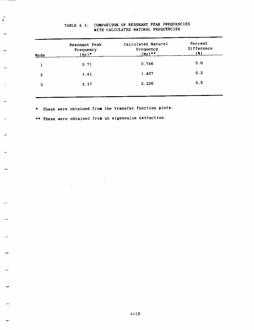
{
TABLE 4.1: COMPARISON OF RESONANT PEAK FREQUENCIES
WITH CALCULATED NATURAL FREQUENCIES
Mode
Resonant Peak
Frequency
(Hz)*
Calculated Natural
Frequency
(Xz)**
Percent
Difference
i 0.71 0.746 5.0
2 1.41 1.407 0.2
3 2.17 2.226 2.5
* These were obtained from the transfer function plots.
** These were obtained from an eigenvalue extraction.
4-10

i 'S,O '
A
i2o _ !I _
L,O --._.,,/ _t tjl
i
_I_, e !
O,O
_,o i,o 2,oi,o i,o _,oi,o i,o 8,oF')_f]- )i2
al) Damage Indicator One Modulus--Damaged
Case
. I
i
I , , i
_[I,_ i _,__I_,-_, ,tII
9"
71_ T
_EO"IlZbl) Damage Indicator One Modulus--
Undamaged Case
Figure 4.5: Comparison of Damage Indicators for Uniform
Global Damage and No Damage for Independent
Base Motions
4-11

_,-W,O_
J
-LIl,ii
O,I
a2)
_*,oe,o _,o 4,o5,e i,o 7,o 3,o_'t_
Damage Indicator One Phase--Damaged
Case
6°'°I ' _ ' ' /'h
4o,o4
_.o,!:o,oi
i-2o,o4
I
i
-6t,t I0,I
I
J
p
_ljl'_'_I,,v' .'. -..". --:
I
I
L1 h
I
[_,0 4,I S,I _,O l,l 8,0
_-_
b2) Damage Indicator One Phase--Undamaged
Case
Figure 4.5 (continued)
4-12

_ 2S,0
N
_0
20,0
m
!5,0
_lO,e
S,t
t,t
il
l tl i
_ii 'i
i /
r
0,0 t,i 2,0
a3) DamageCase
p
I
_I ",. ,d_ m
L ,' "r"_'
_,o4,o5,o_,oi,o8,o
Indicator Two Modu.l.us--Damaged
I_'_i
le,_oi
lt,25._
¢
_,25
IX_M]£- _ _ _ 1_0_2IN_OUT_ _• i i I, _GE i
i i
i_ ,II i
i,i!lI!i i,'' ..
I
o,o s,o _,o _,o i,o _,o _,o i,o _,o_-_
b3) Damage Indicator Two Modulus--Undamaged
Case
Figure 4.5 (continued)
4-13
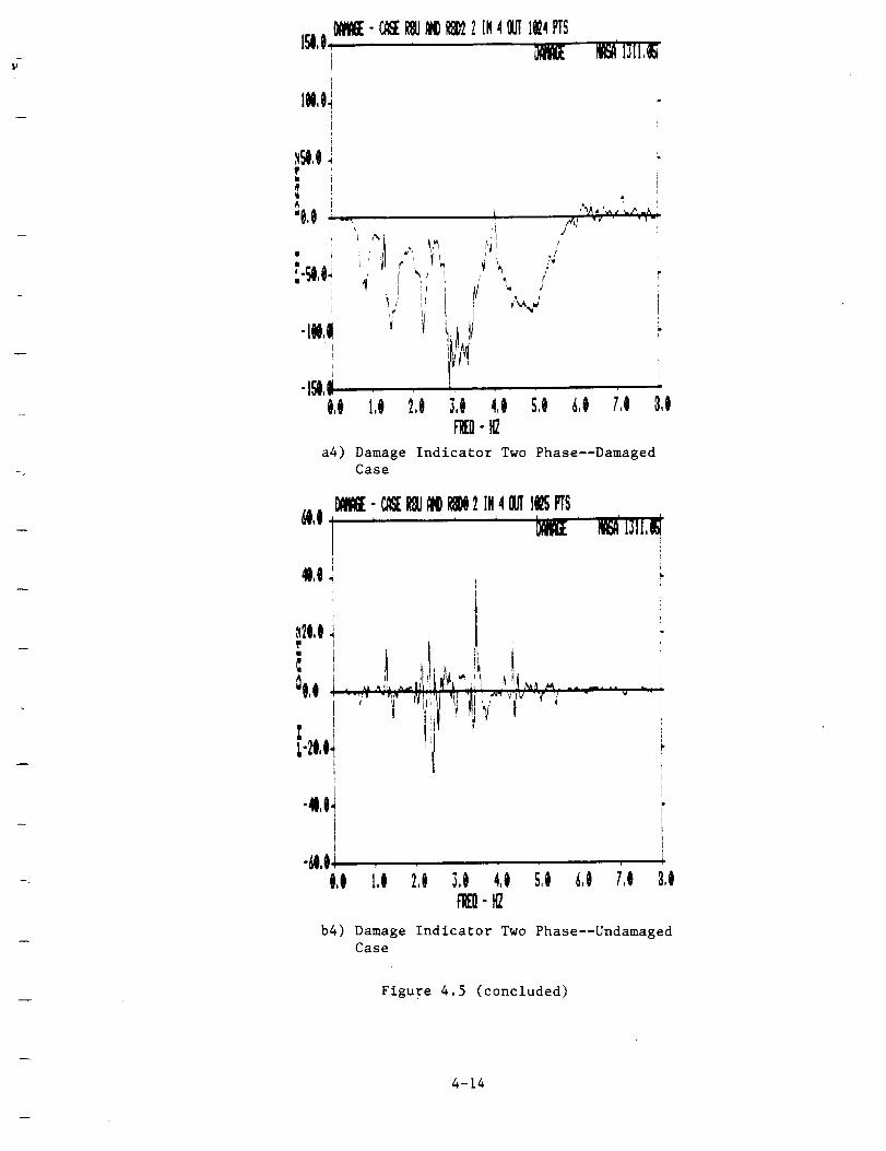
ISl,O
too,o_I
I'm i
++ !^ i
ii
m I
i-_,o!
-LN,IIi
-I_,!O,O
01_- _ _ _ _ 2 IN4_ 1E4PTS
£
"'"_I "_i ;", :_1 :11
? tit
t,O 2_,0 _,0 4,t
_12-H2
i
IP
iti
/ ;'( i
/i
so 6o 7o 8o
a4) Damage Indicator Two Phase--Damaged
Case
O_mE-_Em_e_2 m4OUTIePTS_o,o] , , , , l_' w'ml,m
b
4l,I_ I 'I I
_O,l._T
iI I ,
,I , --,;'_ ......
, "_i' ++ +iir,+ ,, _+9
-21,I,
-41
•.+ "-- i
-+,II +
b4) Damage Indicator Two Phase--Undamaged
Case
Figure 4.5 (concluded)
4-14

peak values of the amplitudes for the two damage indicators was from about
10_ to 115_, with most being above 50_.
In looking at the plots of the damage indicators it is seen that the
amplitude (modulus) peaks greater than one correspond to "undamaged" and
"damaged" natural frequencies for damage indicators D(2) and D(1).
respectively. The peaks for the phase plots occur between the "undamaged"
and "damaged" natural frequencies. This will be discussed further in Section
6.0 (the modal strain energy distribution method of locating damage).
The damage indicators can be used to some degree to quantify the
level of damage in a structural module. For uniform damage, it is possible
to determine the change of a damage indicator peak for a given "undamaged"
natural frequency with a change in the level of damage. Because the level
of uniform damage can be represented by a scalar variable, _, it is possible
to plot a damage indicator level as a function of this variable, i.e.,
u is the fundamental "undamaged"Plot D(2)(f ) as a function of R, where fl'
natural frequency. This was done and is shown by Figure 4.6. Given the
damage indicator level the uniform damage level can be found.
For an actual physical system it would probably be necessary to use a
numerical model of it to obtain an estimate of the functional relationship
between an indicator, at a resonant frequency, and the uniform damage level
variable, X. In determining this relationshlp any possible error inherent
in the model would need to be taken into account--an upper and lower bound
functional relationship would have to be found.
It would be considerably more difficult to determine a functional
relationship between the damage indicator and fraction of local damage than
for uniform damage. This is solely due to the fact that there are an unlim-
ited number of possible different local damage locations or combinations of
locations. Even if essentially all local damage indicator relationships
were known, it would be necessary to know where the local damage was in
order to be able to select the proper relationship. It might be helpful to
divide the module into a few regions and look at the damage as being uniform
within a given region and zero within the others for the case of a single
local damage.
4-15

2.5_
='._ (fl)
2.0_
(f2)
1.5 _
1. I I0 .05 .IO .15 .20 .25
Uniform Damage Scalar, 1
(Fraction of Mass Reduction)
Figure 4.6: Damage Indicator Level as a Function of
the Uniform Damage Scalar
4-16

4.2.2 Truss Structure--Module Approach Using Local Modes
The structure used for this numerical example is shown in Figure 4.7.
It is a 54 degree-of-freedom 2-dimensional system (motion is in the x-y
plane). The excitation is uniform enforced base motion at Nodes 1 and 15
(at left end of structure). The module used starts at Nodes 6 and 20 and
goes to the right to Nodes 14, 10, 24 and 28.
The model structure was designed so there would be global modes whose
elastic motion would be only within the selected module--local modes were
created. Figure 4.8 contains plots of some global and local modes. Table
4.2 is a list of the system's natural frequencies and uniform base motion
participation factors. It can be seen that by using x-dlrectlon base motion
the third mode (a local mode) can be excited very well, while Modes 1, 2, 4,
5 and 6 are essentially not excited. Also, by low-pass filtering the base
excitation at 10 Hz (as was done) it is possible to minimize the excitation
of any modes above 10 Hz. This makes possible the selective excitation of a
local mode, and hence, a single-input slngle-output (SISO) module transfer
function can be calculated easily (see Figure 4.9). s
Using the SISO transfer function within input and output being at Nodes
6 and 9, respectively, the two damage indicators were calculated for a dam-
age case (see Figures 4.10 and 4.11). The comments made concerning the dam-
age.indicators for the previous numerical case hold for this case. Because
of the excitation of only a single mode the shape of the curves for the dam-
age indicators is quite simple as opposed to those for the prior case.
Basically, the concept of a damage indicator is fairly simple. The diffi-
cult thing to do is to correlate the maxima of peaks related to resonances
with the level of module damage.
* What was done for this frame structure can be generalized for some other
structures. However, this approach is not useful for a general structure
because 1) there may not be any local modes with motion in the desired
areas, 2) of possible high modal density of global modes around the local
modes, and 3) for additional reasons, of the inability to excite only
local modes.
4-17

'"I,C¢..J
.,,,-"
a"
.,e"
16 17 IB lg 2_" 2_.C......... T.......... T......... "T'"....... T': .-'T'-. /
I .....-_....._ --,_.....I --._......._-_.....I :.,--i-,<-......."" ""-. i .-'" -" _. x"" "'- .-'" "'"_ ._'" "x .,.-" -w_i..........-.z...........i........--._,......b- --,.i.,---,
"',, L
2E, 2,? ,."'_,.,
2 '-_
I)jt
iF/ I_
Figure 4.7: Numerical Model of a Truss Structure
4-18

1
I'K-.
!
N.... _ iI i...... I I ------+_
",, / I I ....\ J I 1 ."_\t I i ..........,_
Mode 1 -------_.-__ ,-
__..___...___-- _._.. --_____..__..___---_ . ,, ..... ___--...,_-.. /' _ ....... .-" N ..-" ,' "..... -'--- i _, t.'., --.__
.... -' 'i ...... ' t "_' I %.-" I ' --=4.__ 'i ",..-_:.-- .-" , "'-. ," I .-" "- I ..-"--. ".. __.-" ,' _ r I ',
.... _ ........ " :1 -''--.- '1 ,' "-,,. i .,..,- '-. "..._.--,-- r -------_ t i ..I'-.-- / _ ""-,- / i / ---_ , .-.... "-I_" "... _ __---"K ,' -"_"-'-- 'I '/ .......... ', ..'__ "1 ...." -',,i.::_ ___ '-._.__...-" ".. J' .,.." ---.__ '.I _./... 1 .......---..' ..- ...... '..---_\... t ../ ..-_-..",,,:I ,.-" --. I/" ------- ..... _'-----',/ ," I "_• ..." "--. I.." _--- "-: _ .I" / ?;_---_ ',, i "d-2 .-"
',,i \ _"--,K.... ,'",& _ _ --'-W
.0 o2 j /
,,, ..,._,"""
,-"........--.L-"..... "--b/ ".l/ "-.b" ,d.." "-- ,-,....
"-,
"N-,x.
Mode 3
7J
/,/
//
.%
_-,.
i,%,
..." ".,..
.1 ...,. !
/ "'%._ j
L
°.,
• o,,
"-. /""
Figure 4.8: Truss Structure--Mode Shapes
4-19

TABLE4.2: TRUSSSTRUCTUREGLOBALNATURALFREQUENCIESANDPARTICIPATIONFACTORS(UNDAMAGED SYSTEM)
Natural
Frequency
Mode (Hz)*
0 703
4 519
4 932
5 219
8 842
8 855
10.316
13.495
Participation Factor
x-Direction
-0.475 x 10 -6
O. 705 x 10 -s
O. 106 x 102
-0.965 x 10 -s
-0.729 x 10--'
-0.893 x 10 -s
O. 187 x 102
-0.191 x 10 -s
y-Direction
0.189 x 10 a
-0.968 x 101
0.662 x 10 -6
-0.323 x 101
-0.968 x 10 -6
-0.161 x 10 -2
0.112 x 10--'
0.587 x i0 _
4-20

U.I
LI,I
I.I
5,1I
_4,0
t,I
I.I
xwurum n_t_- rime <x_>, +r_wrx/us_1x' ' ' ' _ u' ml,e
I;'JIL1,IIZ
a) Modulus
SLIM/YMMlrlflIIqlBCYIM- _ (X MOT),IIIfd_TX/IILMI_iU,I ' ' ' ' _W uu' lm.u
SO,I
MI,I
_-LOO,g
-LH,I
-2gO,_o,o l,o 2,o 3,o _,o 5,o +,o _.o a,o
!1, 112
b) Phase
Figure 4.9: SISO Module Transfer Function (A9/A6)for Truss Structure
4-21
,+ +.,+.I, _, " ;O_+_+,_:+++-u,..++-+++ ++
01= PO_ +++';_ "

12,1
ILl
I,I
I
Z,II
I,II
smmttnurQ ruNmm-mM <_mot>,,n_t_],nslm' ' ' ' _lol_ HII$1'13LI,i
o.o _., z., 3+.o ,_., +.l +.1 +.oF'Ut, H2
I.I
a) Undamaged Global System--Modulus
i_.ll
il.l
I.II
i
_4.I
Z.I
I.I
Slll,l tMIPD IICIOIq - _ (X I_), AIISIIaJTX/IIIIi'L'X' ' ' ' _+,w++_ram'Lm.,
O.O t'.O Z'.O +'.O 4,0 +,O +.O 'i.O O,OllD, NI
b) Damaged Module--Modulus
Figure 4.10: SISO Module Transfer Function for Two
Damage Levels
OF :'++;+,,:i +++' "+ +_,+"
4-22

LN, I
il.i
-lSl, i
;[Ja_xt_m nmctz_-ntA,om¢xmoOT),,nsoo'_em6_' ' ' ' _lui/_ Hill' L3LL,I
\
-2N,!o.o l.o _.o 3.e _,o _.o _,e _.o
I'll1, il8,i
c) Undamaged Global System--Phase
LN, I
5O,I
Hi, i
_-LN,I
-150,1
Slig_ TMlrllt MCTIOM- _ (X]NOT),liiSImTX/ilSii6_' ' ' ' _r,w_ ms,'ml,e
-m,!o.o L.0 n'.0 3.0 4.0 _'.0 _.0 _,0
rido NI
d) Damaged Module--Phase
Figure 4.10 (concluded)
1,0
4-23
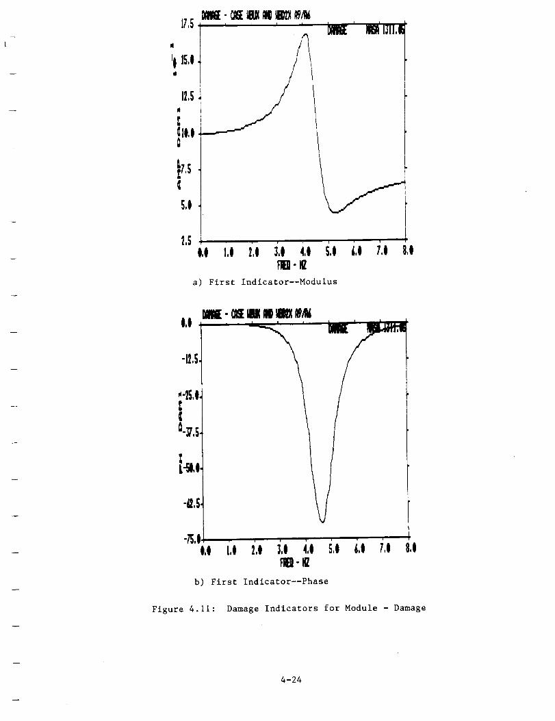
17,5
N
t! 15,!d
it,5
E
tl,l
1
5,!
I I I I
__y
2,5I,I 1,1 ,! ,I 4,1 5,1
a) First Indicator--Modulus
v
i,o 7,o 8o
I,I
_-25,1.X_|_-_,5.
1
L I I .
o,o i,o i,o i,o i,o i o i,o i o 8,o_-_
b) First Indicator--Phase
Figure 4.11: Damage Indicators for Module - Damage
4-24
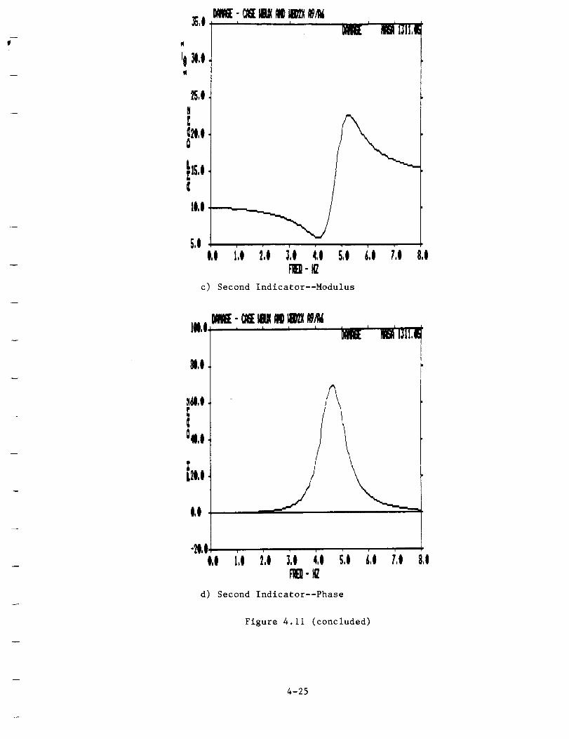
N
rO]I,Iqq
HE
21,I
ILl
+,II,I
c)
III,I
81,I
,_61,Iipiii
|+41,I
I,I
-_,0I,I
' IB' 1311,15
i',0 i,, +',oi,o i,o i,o i,, s,o_-I_
Second Indicator--Modulus
ME - _ IIHIIKm II_ A9_6i i I i
i ' W' I_II,I_
I
lJlJ
d)
t',o i,, i,, i,o i,, i,o i,, 8,oF'HE]-I_
Second Indicator--Phase
Figure 4.11 (concluded)
4-25

A module transfer function was not calculated using global and local
modes for this problem because of the inability to determine it using a
robust approach. It would have been possible to follow the non-robust
approach described at the end of Section 3.0--using forces inside and out-
side of a module and appropriating them, ensuring that the module boundary
does not move for a desired frequency domain.
4-26

5.0 TIHE DOMAIN MODULE MODAL IDENTIFICATION
As mentioned previously in this report (Section 3.0), an approach that
can be used to obtain module modal properties is system identification using
the equations of motion for a module (Equation 3-6 or 3-12). There are
different ways that this problem can be approached. The method used herein
is that developed by Beck [1,2]. Conceptually, it involves determining the
module modal properties (fixed-boundary) that result in a best fit (match)
between the prediction given by Equation 3-13 and the experimental data
(module responses).
His approach was developed for use with civil structures undergoing
seismic (earthquake) excitation--nonuniform enforced base motion. Hence, it
did not include the fi(t) term on the rlght-hand side of Equation 3-13.
However, it is possible to cast the rlght-hand side of the equation into a
form that looks like the corresponding term in the Beck equation. Thus,
conceptually the forces can be treated as though they are a "type" of
boundary motion. Thus, with Beck's approach Implemented in his computer
code MODE-ID, it was straight forward to apply it to the type of problem
addressed In this report. (An example of the prior use of hls method/code
in successfully solving a problem is presented in Appendix F.) In the
following part of thls section, results are presented from the use of the
HODE-ID computer code.
5.1 Space Truss Example Problem
The model structure used for determining if the Beck approach could be
used for a general type of structure/module that might be used in space is
pictured in Figure 5.1. Its first two global mode shapes are given in
Figure 5.2. The module selected for use in the investigation was defined
using Node Points 8 through 22 (see Figure 5.3). The boundary points are
Node Points 8, 9, 10 and 20, 21, 22. The structure was excited by applying
forces at Node Points 11 and 14 and in the y-direction. They were
independent of each other and random/transient traces.
The first identification performed was that of the global system. For
this there were no boundary motlons--Node Points 1 and 29 were fixed
(constrained from movement) for the entire study. It was possible to use
HODE-ID to correctly identify the lower global modes. Thls effort was
5-I
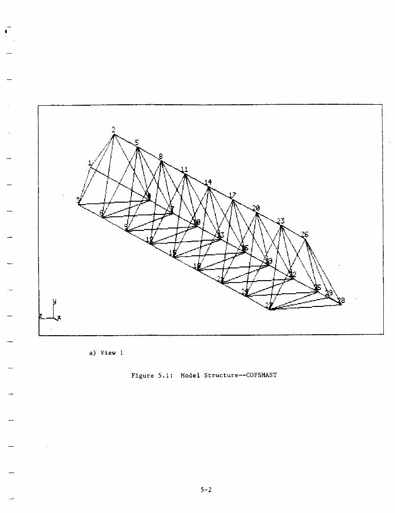
° •*_°
\
\
a) View I
Figure 5.1: Model Structure--COFSMAST
5-2

b) View 2
Figure 5.1 (concluded)
5-3

IIODE • 1
m_
._ • .,_o.
a) First Mode
Figure 5.2: COFSMAST Global Mode Shapes
5-4

MODE: _,i i
b) Second Mode
Figure 5.2 (concluded)
5-5

Figure 5.3: COFSMAST Module Studied
5-6

performed just to verify that MODE-ID could correctly handle forces applied
to the module interior.
The next effort was to determine the fixed boundary undamaged module
modal properties using MODE-ID. The problem inputs were the twelve boundary
motions and two applied forces. The problem outputs were chosen to be the
motions at Node Points 11, 14, 16 and 17 in the y-direction.
Simplistlcally, the program estimates the pseudostatic influence matrix,
-IP = -KiiKib (5-1)
which relates the pseudostatic part of the module response to the boundary
motions by
si = Px b (5-2)
Once this is done the "dynamic" response (relative response) of the module
is found from
r i = x I - s i (5-3)
With this information, the fixed boundary module modal properties are
determined. Actually, this is an iterative parameter estimation process
which alternates between updating the pseudostatic matrix estimates and the
modal parameter estimates.
During the first MODE-ID iteration, the pseudostatic influence matrix
determination resulted in almost a perfect match between the pseudostatic
part of the response of the module and the absolute module response (see
Figure 5.4). Thus, the relative response determined was essentially zero.
This mode is impossible to determine the fixed-boundary module modal
properties. It was found that the identified pseudostatic influence matrix
was very different from that determined from the numerical model--the
identified influence matrix did not just represent the static properties of
the structure. This came about because of 'the large number of boundary
motions being related to each other through the dynamics of the global
system.
To show how different the two pseudostatic influence matrices were, the
corresponding pseudostatic module responses were plotted in Figure 5.5. As
5-7

00
13.
_30
v
>-T"
LI.
0Q
O
c/)U.
00
tJ
0
I'! ,I;
(O=! S/O=lCj/NI) NOI J...VI=I =1-1 q OOV
O
5-8

Q.
n0
v
>_
'I-
!10t_
* a
ii00
,IJ
m _
r/l
,--.t
r_
I I I I I -_.,._._J I I I I Ip
m_
d
I I I "--'7--1"-I I _ I I I
i i
(O3S/O3S/NI) NOI-LVI:1:17 :::IOOV
I tO
O
W
W o
F- °0
04-4
U
U_ .._
I
0
Z
orj
u'h

a0
v
>
LL
00
i o
0
tt
00
0
00_ Q;
0
(03 SlO::::ISIN I) NOIIVW=:173OOV
'0
0(J
-,.1"
u_
Q;
5-10
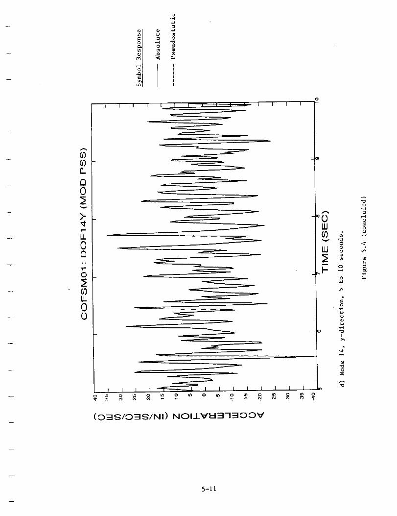
o_
0
_J
0
f_
_J
4.J
0_J,3
0
"0
=
OJ
n
n0
V
T-
LL0D
LL00
I I I t I I f _ I I 1__ t
R
l
L
R
m
t t t
i IO t0
I I I -'=F--'--I__0 U_ 0 _ 0
CO 04 04 _- ,-
t I I I I I I I
0 kO 0 _ 0 LO 0 _ 0
(O3 SIO::::I$1N I) NOIIVEI:=I73OOV
O
Wr,/)
=
LLI o
.. o0
0
(J
LD "0
I
J
0
.,)
,--4
=0
5-11

(/)
n
n0
V
>-I--
I I
LL00
11
cOu.00
h-i
I I I
0
u,_
4 _ _: _: =----"lIr--_-_ L - -_L_ I 1 1
w
mI .I.
I II,_ 0 I,_
I -_-_---T ---_-- I I I I I0 I.O 0 It) 0 _ 0 _ 0
(0::I SIO:ISIN I) NOIIVI::1:1-1 ::IOOV
0
W
V
W
I
.I--
(0
0
0
U
I
0
Z
0
0u_
0
(2
.I.t
0
0 0
0
o ,"
5-12

0O
n
n0
V
>-
LL00i •
LL00
E
_J
I I I I I -f-'_.-..-.z; r I I L I
...-.- _--" - _ _
__air__'=.
"; -- _.-..,._
_ -- _',.---'_-__ _---;;;
I I I I i
0 _ O t_ 0 _ 0 I_ 0 tO 0 U') 0 _ 0
_ _ N _ ...., 7- _, _ _ _,
(03 S/O::IS/NI) NOIIVW=I7=IOOV
OP
_0W0_V
UJ
--D
o
I
0
Z
=
U
=oU
u'h
L_
5-13

I
can be seen, the two pseudostatic responses are very different. What will
tend to happen when this approach is used to identify modes of modules like
the one being studied, is that because of the relationship of the motion of
the many boundary points through the dynamics of the global system, the
identified pseudostatic module response will be able to match the absolute
response close enough so that the module modal properties will not be
determinable. This is discussed further in Appendix F. Also, it is seen in
the example problem below involving damage of the structure.
The global system was damaged only outside of the module. Then the
structure was excited in exactly the same way as before. The module modal
identification was performed using MODE-ID. Comparisons were made between
the pseudostatic and absolute module responses as before (see Figure 5.6).
The two responses were in good agreement, although not as closely as before,
however, the module modal properties could not be determined because the
identified "pseudostatic" response actually incorporated most of the
module's dynamic response_
It should be pointed out that the module modal identification method
implemented in MODE-ID works well for those cases where the modes to be
identified have motions local to the module--the modes motion is contained
largely within the module. The example presented in Appendix F fits into
this category. Even thoug_ the global system was the earth down to bedrock
and the bridge, the bridge elastic modes had their relative motion largely
contained within the domain of the bridge.
5.2 References
1 •
2.
J.L. Beck, "Determining Models of Structures From Earthquake
Records," Report No. EERL 78-01, Earthquake Engineering Research
Laboratory, California Institute of Technology, Pasadena,
California, 1978.
S.D. Werner, J.L. Beck and M.B. Levine, "Seismic Response
Evaluation of Meloland Road Overpass Using 1979 Imperial Valley
Earthquake Records," Earthquake Engineering and Structural
Dynamics, Vol. 15, 249-274 (1987)., John Wiley & Sons, Ltd., 1987.
5-14

LL00
{J
,i,J
,_ "¢1
(0==!£/O=18/NI) NOIIV'I=I =1-1=100,¢
A
0W
LLI
O
,,w
..,=1
I
OZ
rj
0,)
II
0
o_r,4
_J
0
J_
0
m
&l
I==1
I=
=,.-.IO68
I=
O
},,4
Or.,.3
4;u_
=b,O
5-15

COCOQ.
00
v
I-=,
LL00
COLL00
4.-I
C_
_ o
0
p._o -
-w-- --
_ ..---- __
.... ,-'___:_:_
(O3 SIO=::ISIN I) NOII"_'EI=::I7 300V
_0WCOV
W
a
_.,_--
0
-M
l
O
Z
=
=
0
=
-M
5-16

6.0 MODAL STRAIN ENERGY DISTRIBUTION METHOD
One of the methods used to locate module damage, which was investigated
and developed during the Phase I effort, is the "modal strain energy distri-
bution method" (NSEDN) [I]. This method uses the previously developed dam-
age indicators to establish which modes have been effected by the structural
damage. Those modes which have not been effected very much or at all are
used to establish where the damage can only be. The following material con-
sists of I) a review and discussion of the theoretical aspects of the
method, 2) an example of the method, and 3) some conclusions.
6.1 Theoretical Discussion
For thls discussion assume that a damage indicator has been selected
for determining which modes have been affected, and to what degree, by the
damage. To look at the NSEDM, first look at a very simple example. Assume
that the damage indicator shows that two modes, a and b, were totally
unaffected by the damage. This means that the damage can only be at the
locations of zero strain energy for Modes a and b (see Figure 6.1). Some of
the points of zero strain energy are taken to be different for the two
modes. For this example it is easy to determine the location of damage.
For thls simple example it was assumed that the two modes were global module
modes--they involved motion throughout the module. If they had not, all
that could have been said was that the only location the damage could be at
in the domain of Modes a and b motion is at the single point indicated in
Figure 6.1.
Continuing with this simple example, suppose that the damage indicator
shows that Modes a and b have been changed only slightly by the damage.
Thls indicates that there Is not a great amount of damage at or near Modes a
and b points of maximum strain energy. This is probably true for points of
moderate levels of strain energy. However, there could be a sizable amount
of damage near points of zero or low strain energy. For this case it is
still possible to determine a subdomaln which contains the damage somewhere
within it (see Figure 6.2).
If the damage level is only "moderate" it is difficult to locate the
damage by this method. This is because the damage indicator could have the
same amplitude for a mode for moderate-level damage at a high strain energy
6-I
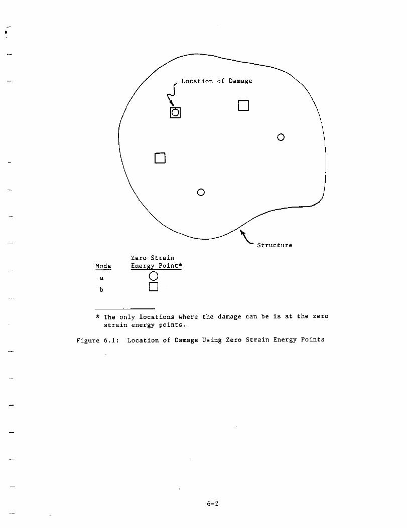
O
Zero Strain
Mode Energy Point *
a O
b O
* The only locations where the damage can be is at the zero
strain energy points.
Figure 6.1: Location of Damage Using Zero Strain Energy Points
6-2

\ _o_\_j_
Structure
Zero Strain
Mode Energy Point
a 0
b [-']
* The high-level damage can only be in the domains within the
dashed closed curves.
Figure 6.2: Location of High-Level Damage Using Near Zero Strain Energy
Points
6-3

point as for high-level damage at a point of medium-level strain energy.
The analysis could be performed, but the best solution achieved might only
be able to indicate a large number of locations, one of which is where the
damage is. Because of this, it will be attempted to locate only
"high-level" damage using the MSEDM.
Using the above ideas, it is possible to derive a simple expression for
the location of high level damage within a module. It is necessary to
determine the modal strain energy distribution (as a function of the spatial
coordinates, i.e., x, y, z) for the modes of a structure. This can be done
best using a finite element model. The procedure followed is to establish
for each mode what its damage level is. If it is hlgh-level, then all that
can be said is that damage could be everywhere. If the damage indicated Is
low-level, then any hlgh-level damage must be near or at the zero or low-
level strain energy elements.
cl and D_ 2, respectively, is defined forA low- and high-level cutoff, Dj
the jt_hhmode. Based on this, the following is defined:
cl all high-level damage is near low-level strain1) if D(_j) _ Dj ,
energy points; and
c2
2) if D(ej) > Dj , high-level damage could be anywhere, where wj
is the jt__hhnatural frequency.
Next, a set is defined for Mode j of finite element numbers correspondinE tod
all those elements where there may be hlgh-level damage, W_.J
d (EJ _ _ maxWj = ekj rjej )(6-1)
where Ek = the kt__helement number (Ek = k).
ekj = the element strain energy for the kt__hhelementand the jth mode.
maxe.
J= the maximum element strain energy for the jth
mode.
6-4

i
I cl
j , D(wj) S 0j
fj =C2
, D(_j) > Dj
gj = a constant factor for the Jth mode.
The solution to the problem of where is the high-level damage located
is found by determining the intersection of sets wd. This can be seen from
J wd--the following. The solution set, I d, is a subset ofJ
dI d c_ Wj (6-2)
From this, it is seen that for the first two modes the solution must lle
d and dwithin the intersection of the two sets WI W2 (see Figure 6.3)--
d dI d c_ W 1 n W2
dThe next set, W_3, can be combined with the intersection of the first two
sets in the same way. Thus,
ld d dI d c (W n W2)n W3
Finally, the solution is found to be
Id = (***((wdn wd) n wd)n***)n Wdn
nd
Id = n Wj (6-3)J=l
where I d = the set of element numbers corresponding to all the
elements which were damaged to a high level.
Several things should be noted concerning the solutlon given by
Equation 6-3. The set found will reference all the damaged elements.
However, there may be element numbers in the set for which the corresponding
elements are not damaged. This problem can be minimized by increasing
the number of modes used. Another problem that can arise is when the module
6-5

* The intersection of the sets is indicated by the
cross-hatched portion.
Figure 6.3: The Intersection of the Sets for Modes One and Two
6-6

has a high degree of structural symmetry. This will be looked at in the
case study presented herein. Lastly, the values for the gj must be selected.
This is not a straight forward task. As can be seen, the MSEDN is not purely
quantitative. The threshold parameters D ci. must be selected in a quali-J
tative/quantitattve manner. Questions must be dealt with such as the
following:
1) how high should the low-level cutoff be so that when the peak
damage indicator value for a mode is less than it, that it can beassured that there is not any high-level damage at high-or
moderate-level strain energy points for the mode;
2) how low should the high-level cut off be so that information is not
lost by calling a "low-level peak" (one indicating no high-level
damage at high-level strain energy points) a "hlgh-level peak" (one
indicating that the damage is so severe that it could be anywhere);
and
3) how is local damage dealt with for a large variety of possible
damage locations--how are the cutoffs dealt with? These issues
were dealt with in a simple way for the case study.
6.2 Case Study
The study discussed in this section involves the numerical analysis of
a simply supported uniform straight two-dimensional beam (see Figure 6.4).
The modal strain energy distribution, el, for this beam was calculated
analytically and is given by
1 (dZ'l (x) / '
where _i(x) is the tth mode.
Once thls was done, the beam was partitioned into segments of equal length
and the strain energy computed for each one for each mode. These discrete
modal energy distributions were used to locate the damage in the beam.
A computer code implementing the NSEDN was developed (described in
Appendix G) and used to analyze thls problem. The results for two of the
damaged conditions are presented below. The first case involved having
large damage within only Segment 22. Sixty beam segments were used to
define the strain energy distribution (see Appendix H). Twelve modes
6-7

x
* The pinned connection restrains translational motion at the pin,
but allows rotational motion in the x-y plane.
Figure 6.4: Simple Case Study--Uniform Pinned-Pinned Beam
6-8

$ SIMPLY SUPF'ORTED BEAM
DAMAGE FILE USED : DAMOUT4.DD
DAMAGE TITLE : DAMAGE AT N = 0.35 (LARGE)
NUMBER OF MODES : 12
NUMBER OF ELEMENTS : 60
DAMAGE FRACTION : .3500
MODE MAXIMUM ELEMENT ELEMENT
NO. STRAIN ENERGY NO.
I 1. O()OE+ 00 31
1. O00E+O0 45
3 I. O00E+O0 31
4 1. O()OE+O() 38
5 I. O00E+O0 31
b 1. O00E+O0 45
7 1. O00E÷O0 _._.'_
8 1•oor)E+O0 34
9 1. O00E+O0 17
I0 I. O00E+O0 45
11 1. O00E+O0 25
12 1. O00E+O0 38
Page I of 3
Figure 6.5: MSEDM Applied to Simply Supported Beam--Damage inSegment 22, Damage Fraction is 0.35
6-9

SIMPLY SUPPORTED BEAM
DAMAGE FILE USED : DAMOUT4.DD
DAMAGE TITLE : DAMAGE AT N = 0.35 (LARGE)
NUMBER OF MODES : 12
NUMBER OF ELEMENTS : &O
DAMAGE FRACTION : .3500
ELEMENT DAMAGE SUMMARY
ELEMENT MODE
NO. NO.
1 2 3 4 5 6 7 8 9 10 11 12
I :.,' ;< X :< :< X X X :',' X X X
2 X X X X X X X X X
3 :_ X X '.i X X X X
4 x X X :_ X X X X
5 :< _: X 'K × :_ K X
7 x x x x x x x x x x
8 x :< X :_ X X X X X
9 x x x x '." :_ X X x
10 :_ x x x x x )¢ x
II x x x x x x x x x
12 X '4 X x x x x x X
13 x x x x x x x x
I 4 x x x x x x x x
15 x x x x x x x x x
16 x x x x x x x x x
17 x x x x x x x x x
18 x x x x x x x x
1 9 x X x x x _" x x x
20 .x x x x x x _" x x x
21 :.,' x x x × x x :< :< X
22 x x x x x x x x x x x
23 x x x x x '4 x :4 _.: x
24 ;< x x x x x x :.', x
25 x x _; x ": x '_
26 x x X x :': '_ X x
27 x x x x x ,,., :.: × x
28 i< x x >" x x x :." x
2 9 '.,' x x x x x ;.: x
0 X :< X X P: _ Y X X
31 x x x × x x >" :4 x
•"_. Y X._,_ X X X :" X >'
3 ."S, x X ,_' X :'" >,' :." X :,_
4, X X X X X ;< :< X }.,'
._,"T5 X × X :< }': :._ X X
3 6 x '4 x v x x >'
3 7 x '4 :." x _' x :-: x x
;_8 x Y '.: x >: x x '.: x ,'_
3 9 }.: }.,' ;-" x x :,' :< x x x x
4 0 x x v x :4 x _" X X X
Page 2 of 3
POSSIBLE
DAMAGE
YES
NO
NO
NO
NO
NO
NO
NO
NO
NO
NO
NO
NO
NO
NO
NO
NO
NO
NO
NO
NO
NO
NO
NO
NO
NO
NO
NO
NO
NO
NO
NO
NO
NO
NO
NO
NO
NO
NO
NO
x indicates possible modal element damage
Figure 6.5 (continued)
6-I0

SIMPLY SUPPORTED BEAM
DAMAGE FILE USED : DAMOUT4.DD
DAMAGE TITLE : DAMAGE AT N = 0.35 (LARGE)
NUMBER OF MODES : 12
NUMBER OF ELEMENTS : bO
DAMAGE FRACTION : .3500
ELEMENT DAMAGE SUMMARY
ELEMENT MODE
NO. NO.
I 2 ._," 4 5 6 7 8 9 10 11 1_
4 i x x x x x x :.( x >( ',<
4 2 v x X x X ;" x ;.( i.,"
4 3 ;._ ;< ;., ,, ;.; ;< ;< ,v
4 4 X ;." x _ ;< x ;< x x
45 '< x x x x ;4 x x x
4 6 %' • x ;.," ;._ ;.( x :_ x ;"
4 7 x x × >' x ;< ;',' ;<
48 x x x '< x x '< x
4 9 x ;.,' x ;< x ,x ;< × >:
50 x x x x x x x :< x
5 1 x x x x x x x x
52 x x x x x x x x x
53 x x x x x x x x x
54 x x :< x x x x x X x
55 x x x x x x x x x
5& x x x x x x x x
57 x x x x x x x x
58 x x x x x x x x
5 9 ;_ x x x >' x x x x
_0 x x '< x x ;4 x x x x x x
Page .3 of 3
F'OSSIDLE
DAMAGE
NONO
NONO
NONO
NONO
NONO
NONO
NO
NONO
NO
NONO
NO
YES
x indicates possible modal element damage
Figure 6.5 (concluded)
6-11

I
were used to represent the beam motion. Only one cutoff was used with the
damage indicator--the low-and high-level cutoffs were taken to be equal.
Also, the constant factor gj was taken to be the same for a11 modes (called
"damage fraction" In the computer code). Figure 6.5 is an output listing
for a damage fraction of 0.35. It is indicated that there may be damage in
Segments 1 and 60. This occurred because the beam end segments saw
virtually no bending. This lead to there being essentially no strain
energy in these segments for all the modes. Thus, these two element numbers
dappeared in all of the sets W_. Thus, they were in the intersection of the
d This is a problem withJ the MSEDM--damage will always be predictedsets Wj.
to be at locations where the modal strain energy is zero for all modes.
Eliminating the beam end segments from consideration, it is seen that
no solution was determined for gj = g = 0.35. It was decided to try to
obtain a solution for g = 0.45. The results are given in Figure 6.6. As
can be seen the solution indicates that there is damage in Segment 22. This
result is correct, however, damage is also indicated to be in Element 39.
This occurred because of the symmetry in the problem. There appears to be
no resolution to this problem. For modules that are not highly symmetrical,
this problem may not occur. Omitting the two problems just discussed, it
appears that the MSEDM is reasonably accurate.
Another case was looked at with damage in two locations--damage in
Segments 15 and 30. The results are given in Figure 6.7. The results are
similar to those obtained for the previous case--the damage was located,
however, undamaged locations were obtained also.
6.3 References
1. "Providing Structural Modules With Self-lntegrity Monitoring," ANCO
Engineers, Inc., final report to NASA, Number 1311.05, May 1985.
6-12

SIMPLY SUPPORTEDBEAMDAMAGEFILE USED : DAMOUT4.DDDAMAGETITLE : DAMAGEAT N = 0.35 (LARGE)NUMBEROF MODES: 12NUMBEROF ELEMENTS: 60DAMAGEFRACTION t .4500
MODE MAXIMUMELEMENT ELEMENTNO. STRAIN ENERGY NO.
1 1.0c)OE+O0 312 1.000E+O0 45
3 1.000E+Oc) 31
4 1.000E÷O0 38
5 1.000E÷O0 31
6 1.000E+O0 45
7 1.000E÷O0 22
8 1.000E+00 34
9 1.000E+O0 17
10 1.000E÷O0 45
11 1.000E+O0 25
12 1.000E÷00 38
Page I of 3
Figure 6.6: MSEDM Applied to Simply Supported Beam--Damage inSection 22, Damage Fraction is 0.45
6-13

SIMPLY SUPPORTEDBEAMDAMAGEFILE USED : DAMOUT4.DDDAMAGETITLE : DAMAGEAT N = 0.35 (LARGE)NUMBEROF MODES: 12NUMBEROF ELEMENTS: 60DAMAGEFRACTION : .450c)
ELEMENTDAMAGESUMMARY
ELEMENT MODENO. NO.
1 2 3 4 5 6 7 8 9 10 I 11 x x x x ',4 x ',4 x x x x2 x x x >' x x x x x x
3 x x '_ x x x x
4 x x x _ x x x
5 x x x _." × :" _ x
x x x x x x x x
7 x x '4 '4 × :4 X _ '4
B x x x x x x x x
x X x x x :4 x :4
I c) x x x x x :4 x
1 1 x x x x x x x x
12 x x x x x x x x
13 x x x x x x x
14 x x x x x x x x
15 x x x x x x x x
16 x x x x x x x x x
17 x x x x x x x x x
18 x x x x x :4 x x
19 x x x x x x x x x20 x x x x x x x x x
21 x x x x x x x x x
22 x x x x x x x x x x x
2_ X x x x X x x x x
24 x x x x x x x x
25 x x x x x x x26 x x x x x x x
27 x x x x x x x x
28 x x x x x x x x
29 x x x x x x x x x
30 x x x x x x x x
31 x x x x x x x x
32 x x x x x x x x x
3_ x x x x x x x x
34 x x x x x x x x35 x x x x :4 x x
3_ x x x x x x ,4
37 x x x x x x x x
38 x x x x x x x x x
_9 x x x x x x x x x :4 :4
40 x x x x x x :,: '4 x
12
x
x
x
x
x
X
x
x
X
x
X
x
X
x
X
x
x
X
x
x
x
X
x
x
x
x
x
x
x
x
x
x
x
x
x
x
x
Page 2 oT 3
POSSIBLE
DAMAGE
YES
NO
NO
NO
NO
NO
NO
NO
NO
NO
NO
NO
NO
NO
NO
NO
NO
NO
NO
NO
NO
YES
NO
NO
NO
NO
NO
NO
NO
NO
NO
NO
NO
NO
NO
NO
NO
NO
YES
NO
x indicates possible modal element damage
Figure 6,6 (continued)
6-14

SIMPLY SUPPORTEDBEAMDAMAGEFILE USED : DAMOUT4.DDDAMAGETITLE : DAMAGEAT N = 0.35 (LARGE)NUMBEROF MODES: 12NUMBEROF ELEMENTS: bODAMAGEFRACTION : .4500
ELEMENTDAMAGESUMMARY
ELEMENT MODENO. NO.
1 2 3 4 5 8 7 8 9 10 i I 1241 x x x x :.: x x x x x42 X x x x x x x x x x43 x x x x x x x x x44 x x x x x x x x x x
45 x x x x x x x x x x
46 x x x x x x x x x
47 x x x x x x x x x
48 x x x x x x x x
49 x x x x x x x x x
50 x x x x x x x x x
51 x x x x x x x x
52 x x x x x x x x53 x x x x x x x x x
54 x x x x x x x x x x
55 x x x x x x x x x
56 x x x x x x x x x
57 x x x x x x x x
58 x x x x x x x x5_ x x x x x x x x x x x
60 x x x x x X x x x x x x
Page 3 of 3
POSSIBLE
DAMAGE
NO
NO
NO
NO
NO
NO
NO
NO
NO
NO
NO
NO
NO
NO
NO
NO
NO
NO
NO
YES
x indicates possible modal element damage
Figure 6.6 (concluded)
6-15

SIMPLY SUPPORTEDBEAMDAMAGEFILE USED : DAMOUT3.DDDAMAGETITLE : DAMAGEAT N = C).25 AND AT N = 0.5NUMBEROF MODES: 12NUMBEROF ELEMENTS: 60DAMAGEFRACTION ! .4000
MODE MAXIMUM ELEMENT ELEMENT
NO. STRAIN ENERGY NO.
1 1. O00E+O0 31
2 i. O00E+c)O 45
3 1. C)c)OE+O0 314 i. OOC_E+C_O 38
5 i. O00E+O0 31
6 1. O00E+O0 45
7 1. O00E+O0 22
8 I. O00E+O0 34
9 I. c)OOE_-O0 17
I0 I. O00E+O0 45
11 1. C)OOE+Oc) 25
12 I. O00E+O0 38
Page i of 3
Figure 6.7: MSEDM Applied to Simply Supported Beam--Damage in
Segments 15 and 30, Damage Fraction is 0.40
6-16
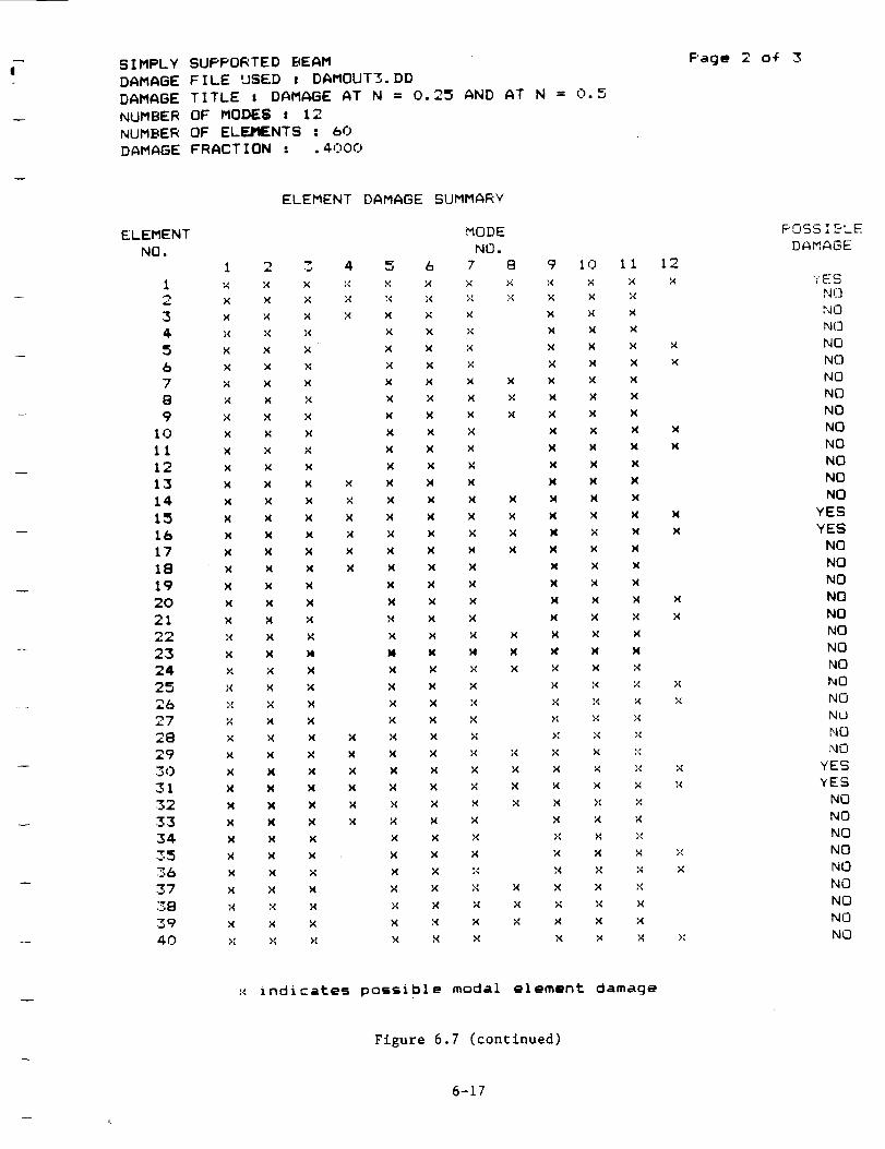
! SIMPLY SUPPORTED BEAM
DAMAGE FILE USED : DAMOUT3. DD
DAMAGE TITLE : DAMAGE AT N = 0.25 AND AT N = 0.5
NUMBER OF MODES : 12
NUMBER OF ELEMENTS : 60
DAMAGE FRACTION : .4000
ELEMENT DAMAGE SUMMARY
ELEMENT MODE
NO. NO.
I 2 3 4 5 6 7 8 9 10 i i 12
1 x x x >" x x x x x x x x
x x x x x x x Y, x x "_
3 x x x x x x x x x x
4 _4 :_ x × x x x x x
5 x x x x x × x x x x
6 x x >. x x >_ x x x x
7 x x x x x x x x x x
8 x x x x x x x x x x
9 x x x x x x x x x x
lO x x x x x x x x x x
11 x x x x x x x x x x
12 x x x x x x x x x
13 x x x x x x x x x x
14 x x x × x x x x x x x
15 X x x x x x x x X x _ X
16 x x x x x x x x X x x x
17 x x x x x x x x x x x
18 x x x x x x x x x x
19 x x x x x x x x x
20 x x x x x x x x x x
21 x x x x x x x x x x
22 :4 x x x x x x x x x
23 x x M _ K x x w x x
24 × x x x × × x x x x
25 ;_ x )4 x x x x ,,{ >" >,'
26 :." '4 x x x "4 x x x x
27 x x x x x x >" ;4 x
2 8 x x X x x x x >" x x
2 9 x x x x x x x x x x :<
3 0 x x x x x x x x x x '4 x
31 x x x x x x x x x x x :4
_ x X X x x x x x x X >'
_3 x ;4 x x x x × x x x
3 A x x x x x x x x :._
35 x x x X x x ?_ x x >:
36 x x x x x :.' :4 x :4 ×
37 x x x x x x x x x >:
3B x :4 :4 >: x x x X x x
39 x x x x x x x x x x
4 0 >" >" _" x x x x x x >:
F'age 2 of 3
POSSI_LE
DAMAGE
""ES
N(]
NO
NO
NO
NO
NO
NO
NO
NO
NO
NO
NO
NO
YES
YES
NO
NO
NO
NO
NO
NO
NO
NO
NO
NO
NO
NO
hid
YES
YES
NO
NO
NO
NO
NO
NO
NO
NO
NO
x indicates possible modal element damage
Figure 6.7 (continued)
6-17

fSIMPLY SUPPORTED BEAM
DAMAGE FILE USED : DAMOUT3.DD
DAMAGE TITLE : DAMAGE AT N = 0.25 AND AT N = 0.5NUMBER OF MODES : 12
NUMBER OF ELL3MENTS : bO
DAMAGE FRACTION = .4000
ELEMENT DAMAGE SUMMARY
ELEMENT MODE
NO. NO.
I 2 3 4 5 b 7 S 9 I0 1 1 12
41 x x x x x x x x x ×
4 _ >," ": '< I._ >,' X x >: -<
43 x :< ;; >: ,.: ,'4 ,%' i< x x
4 4 x x ;,: ;< ,,< ,< >_ :4 >, :4 X
45 x x _4 ;.( >_ ,_ A' ;4 A A >( x
4_ R x x >_ x >_ x y, x >( x x
4 7 x x x x x x x _ :_ x x
48 x x x _< ;.,, ,,.,, x i4 _4 x
4 9 x x x x x x x x x
50 >" "_ "< X 1,_ >," ;4 x X x
51 x >4 x '4 x x x x X X
52 x >: x x x × x x x x
53 x x :4 x x x x x x x
5 4 :4 x >' :4 x x x x x x
55 x x x x x x x x x x
57 x x x x x x x I., x
58 x X x ;4 >4 x >4 X >_ x
5 _ :< ,_ x x x x x x x >: X
6 0 x ",4 X X M X X X X x X X
x indicates possible modal element damage
Figure 6.7 (continued)
Page 3 04 3
POSSIBLE
DAMAGE
rio
NO
NO
NO
YES
YES
NO
NO
NO
NO
NO
NO
NO
NO
NO
NO
NO
NO
NO
YES
6-18

d
DAMAGE FILENAME : DAMOUT3. DD
DAMAGE AT N = 0.25 AND AT N = 0.5
NUMBER OF MODES : 12
MODE D(W) Dcrit (W)
1 100. 000 10.00()
2 1()0. 000 10. 000
3 IO0. 000 i0.00()
4 I. 000 I0.00()
5 10C). OC)O l0. 0006 IOC). 000 i0. 000
7 100. 000 IC).OOC)
8 i. 000 I0. 0009 I00. 000 iO. C)C)O
1C) 10C). C)O0 10. OC)O11 IOC). OC)O 1C). OOC)
12 1. C)O0 10. C)O0
Figure 6.7 (concluded)
6-19

7.0 SYSTEM IDENTIFICATION AS A METHOD OF LOCATING DAMAGE
System identification, SID, can be used as a tool to help determine if
a structure has been damaged, and if so, where. The part of SID that is
being referred to here is parameter estimation. In general, a parameter
estimation method involves defining an objective function which expresses
the difference between the predicted and experimental response of a system.
The objective function is dependent only on the parameters ("constants")
that are used to define the mathematical model of the system, e.g.,
thickness and density of plate components. The task is then to minimize the
error in the prediction model. This is done by finding the model parameter
values that correspond to a minimum extremum of the objective function.
Different parameter estimation schemes use various types of objective
functions and various methods for finding a minimum of objective function.
Part of parameter estimation involves establishing the uncertainty in the
experimental data and the uncertainty in the original estimates of the model
parameters. Overall, system identification deals with identifying
(characterizing) a physical system with a mathematical model using
experimental data and one or more system identification analysis procedures
[1].
In applying SID to the damage detection problem herein, the responses
consist of the elements of the module transfer function matrix. (Of course,
they could have been other variables such as the acceleration or strain at
internal points of a structural module.) The model parameters are the
constants which are used to define the element properties.
The good aspects of this type of approach are (1) the occurrence of
damage, the determination of its location, and its extent (quantitative
value) are determined, (2) for some cases the damage can be substantial and
its quantitative value can still be determined with a reasonable degree of
accuracy, and (3) the various basic numerical algorithms associated with
this approach are well established and software implementing them can be
written in a straight forward manner [2]. The drawbacks to using the method
are 1) uniqueness of the solution cannot be assured--there can be other
local minima besides the one which is sought, and one of these minima might
be found, 2) the algorithms might work well for many different cases (i.e.,
different structures, damage situations), but for some others they may not
7-I

work well, and 3) a considerable amount of numerical effort (large computing
times) can be required to find the solution.
The methods selected for implementation here are described in Reference
2. The objective function defined is based on Bayes Theorem. Hence, the
method of SID used is called Bayesian Parameter Estimation. The algorithms
developed for use in finding a minimum of the objective function is based on
the Newton-Raphson minimization algorithm. Various modifications/enhance-
ments can be made to these algorithms which would help in finding the
desired minimum [3].
An important part of solving the SID problem is the determination of
the sensitivity matrix, S. The elements of it are given by
Sjk = 8Rj/Sp k (7-1)
where R. = the jth model response variable (i.e., an eigenvalue).l
Pk = the kt__hhmodel parameter.
For this problem the model responses are elements of the module transfer
function matrix (t4TFM). There are two basic approaches for determining the
MTFM; they are 1) "dlrect"--determine the matrix from the inversion of the
power/cross-spectral matrix [4] and 2) "modal approach"--determine the
matrix from the module modal parameters. If the former approach is used,
the sensitivity matrix would have to be determined using finite differences-
-determine the t4TFM corresponding to at least two different model parameter
states and approximate the sensitivities using a finite difference approach
to estimating a derivative (i.e., central difference). This method is very
computation intensive.
It may be preferable to determine the MTFM from the module modal
properties. Given an expression for the NTFM as an explicit function of the
module modal properties, it is possible to differentiate it with respect to
the model parameters.
Hij = Hij(_k' _k .... )
7-2

where Hlj
_k
Sk
P!
= an element of the MTFM.
= _k(Pl) is the kt_hh module natural frequency.
= _k(Pf) is the kt_hhmodule mode (a vector).
= the Jth model parameter.
aP! k aek aPl m,k a_bmk 8P!
4- . ° . (7-2)
Also, it can be shown that [5]
aPj 2_k *k - _ _ *k(7-3)
and [6]
_.-Iz - _i) aPj aPj - _p---_i *k(7-4)
Equations 7-3 and 7-4 can be used along with Equation 7-2 to efficiently
determine the required sensitivity matrix. In doing this, it is necessary
to evaluate the derivative of the global stiffness and mass matrices with
respect to each of the model parameters. This can be done using finite
differences, perturbation techniques, or by developing an analytical
expression for each element matrix and then assemble them to obtain the
corresponding global matrix.
In preparation to performing the SID as described above, a simpler SID
was performed using the system natural frequencies as the model responses.
The system analyzed was a pinned-pinned straight two-dimensional beam. The
SID to locate the damage was done using ASTRO/MOVE [5]*. In its "undamaged"
state, the model was a uniform beam. The model was "damaged" by changing
the cross-sectlon moment of inertia for a few beam elements. Natural
* ASTRO/MOVE is a linear static and dynamic finite element computer code
which can be used to perform nonlinear parameter estimation in an
automated manner. It was developed by ANCO Engineers, Inc.
7-3

q
frequencies corresponding to the damaged state were determined--these were
called "data". It was then determined, using SID, which elements had their
moment of inertia changed ("damaged"). This worked well, as expected--the
"damaged" elements were located. A few problems were encountered (it was
not surprising), but they were easily dealt with. The kinds of problems
encountered will be discussed in general in the recommendations in this
section.
The next step taken was to include the system modes with the natural
frequencies as making up the model responses. The same problem was rerun.
However, even with a great deal of effort it was not possible to obtain any
solution--the SID process never converged to a solution. It was concluded
that ASTRO/MOVE probably has coding errors in it associated with the mode
derivatives with respect to the beam element property constants. At this
point the SID process was not investigated further.
Other SID projects have been performed by ANCO where the model
responses included natural frequencies, mode components and acceleration
response quantities, and the desired results obtained. This was done using
a different ANCO SID computer code--NONBAY. However, this code uses the
finite difference approach to calculating the response derivatives and is
very laborious to use. For this reason, this code was not used to further
the research.
Because this later code gave good results it is known that SID can be
satisfactorily performed using all modal parameters as model responses.
Thus, a SID process using the elements of the NTFM as model response should
work well, as long as the usual problems encountered in performing SID can
be dealt with adequately.
9.1 A Few Recommendations for Performing System
Identification To Detect Damage
There are a great number of recommendation/guidelines and things to be
cautious about in performing system identification that could be discussed
herein. Many of these are already documented in a variety of papers on SID.
The only recommendations discussed herein are those which perhaps have a
special bearing on damage detection for complex structures. They are
discussed below.
7-4

It is important to minimize the number of model parameters. This is a
sound practice that should be followed in performing any SID task. However,
this is even more important when the structure is very complex, such as the
space station. Even if the modular/substructure approach is used, many of
the modules could be very complex themselves (hundreds of structural
members). For this case it is necessary to use only a few module model
parameters relative to the total number of parameters that could be used
(hundreds of parameters corresponding to the truss cross-section
properties).
One way this can be done is to "divide" a module into substructures. A
single stiffness and mass parameter could be defined for each substructure.
The stiffness and mass of a substructure would be modified by changing only
their respective multiplicative factor, i.e.,
K (r) = k(r)K (r)s U
M (r) = k(r)M (r)m u
where g,r,,M,r,I _ ; t = the stiffness and mass matrix for the rth
substructure, respectively.
u = refers to the undamaged state.
k(r),k (r"_ = rth substructure model parameters correspondingS m
to the stiffness and mass of the substructure,
respectively.
Of course it is important to not make the substructures too small or too
large.
When the damage level is high (a situation where it would be important
to detect it), it may be difficult to find the solution to the problem using
system identification--it may be difficult to find the correct local minima.
Sometimes a solution may never be found. To minimize this type of problem
it is important to have as much information about the module as possible
(many natural frequencies as opposed to a few). Also, if any visual
observations could be made and broken (badly damaged) members identified,
this information could be used in obtaining a solution. Lastly, it may be
helpful to extend the convergence domain to minimize any divergence problems
[3].
7-5

7.2 References
1 .
2.
3.
4.
5,
6.
B.J. Hsieh, C.A. Kot and M.G. Srinivasan, "Evaluation of System
Identification Methodology and Application", ANL-83-38, Argonne
National Laboratory, May 1983.
"Providing Structural Modules With Self-Integrlty Monitoring", ANCO
Engineers, Inc. Final Report 1311.05 prepared for NASA, May 1985.
M. Aoki, "Introduction to Optimization Techniques - Fundamentals
And Applications of Nonlinear Programming", The MacMillan Co., New
York, 1971.
R.K. Otnes and L. Enochson, "Digital Time Series Analysis", John
Wiley and Sons, New York, 1972.
"ASTRO/MOVE User's Manual", ANCO Engineers, Inc., Culver City,California 90232.
R.B. Nelson, "Simplified Calculation of Eigenvector Derivatives",
AIAA Journal, Vol. 14, No. 9, September 1976.
7-6

8.0 SELF-INTEGRITY MONITORING HARDWARE SYSTEM
8.1 Functional Requirements
The function of the Self-Integrity Monitoring System is to detect
damage that may have occurred to the structure of the Space Station and
report its extent and location.
This will be accomplished by sampling vibration signals sensed by
accelerometers, comparing their characteristics to previously established
parameters and analyzing and reporting differences.
The Data Acquisition and Processing System (DAPS) performs these
sampling and analyzing tasks. Its major modules are:
a. Host Processor System (HPS)
b. Satellite Processor Systems (SPS)
c. Inter-Processor Communication Loops (ICL)
d. Data Acquisitlon-Signal Conditioning Modules (DASC)
e. Sensors and Cables
f. Software
The integration of these hardware and software modules forms the PAPS
system. Reporting will be via communications link to an existing Space
Station Computer (SSC) system that will provide the DAPS system with
astronaut interactive capability. A simplified block diagram of the DAPS
architecture is shown in Figure 8.1.
The frequency of the PAPS monitoring cycle has a marked influence on
the functional requirements. In addition to data sampling frequency having
a direct relationship to power consumption the cyclical heating and cooling
of the various structural elements being monitored will dramatically impact
the validity of data being received from the sensors unless adequate
safeguards are adopted.
Ideally, monitoring should be conducted when the sensors and their
associated structural members are exposed to the same environmental heating/
cooling that prevailed when the "base-line" readings were obtained. This

o
zI
I,--Iw¢t)
OZ0oO0OF-w,<
._. 0 00--
zo_.l
I
=
e-
e_
,o
=;
i °_
8-2

can be achieved by arranging for the monitoring cycle to coincide with the
orbit and attitude of the Space Station.
Temperature stabilization requirements are examined in detail in
Section 8.3.
It has been concluded that to obtain adequate transducer response the
Space Station structure will require artificial excitation although
initially it was considered possible that the DAPS system might be capable
of detecting damage/degradation in the structure by sensing changes in
responses to natural stimuli.
Experimentation will be conducted during the design phase to determine
the optimum frequency and magnitude of structural excitation that meets both
the PAPS requirements and constraints imposed by station operational
.considerations.
Excitation signals wlll be generated by the SPS systems and used to
modulate power to vibrators mounted on the structure. A special output
channel will be necessary in the DASC module to provide this capability.
8.2 DAPS Architecture
8.2.1 Hardware
Details of a typical HPS-SPS-ICL arrangement are shown in the
simplified block diagram Figure 8.2. The basic system design allows one HPS
system to support a quantity of SPS systems by multiplexing data over dual
communication loops.
A loop configuration has been selected for the satellite
communication network, to provide a high degree of reliability to this
critical system element. Although a more complex arrangement both from a
hardware and software standpoint than the "Star" arrangement originally
proposed in the Phase I study, the need for redundancy throughout the PAPS
system is manifest and the provision of duplicate hardware in this and other
difficult to service system elements is mandatory.
This architecture permits satellites to be polled from either end of
the loop so that the system may continue to operate effectively in the
8-3 iq,,'E(.:EI3!i_ji'.-'U_,L.._'..:'.:_'I'LL;'_,r{L_',jI_.O

0 _1 ._1< 0 0
¢J0
-M
Ir._
I
ooC'4
8-4

event of a communication link malfunction. The paired satellite processors
will each be assigned to separate loops thereby permitting a processor
disconnected by a loop hardware failure to be addressed via the healthy loop
and the interprocessor link.
It is proposed to use fiber optic cables for HPS and SPS
communications. These are in common usage in terrestrial distributed
architecture data acquisition systems providing low loss, reliable, "noise"
immune data links.
This choice will be reviewed during the detailed design phase when
their suitability for use in a space environment, the availability of
suitable Data Loop Couplers, and the practicality of using current optical
cable termination techniques in a EVA environment will aIl require further
evaluation.
If conventional cables are used for the data links, it is important
that effective shielding and grounding techniques are used to ensure data is
not compromised by noise or ground loops.
8.2.1.1 Host Processor System
The Host subsystem is composed of the Processor Module and the Data
Loop Controller Module.
A candidate microcomputer for both the Host and Satellite
subsystems is the 8095, a member of the INTEL MCS-96 family. These are
powerful single chip 16-bit processors that are tightly coupled with
program and data memory. They support bit, byte, and word operations. Long
word operations are also supported for a subset of the instruction set.
With a 12 MHz clock frequency the device can perform a 16-bit addition in
1.0 micro-sec and 16 x 16 multiply or 32/16 divide in 6.25 micro-sec.
Also provided on-chlp, are a serial port, a watchdog timer, and a
pulse width modulated output signal. In addition, an optional on-chip A/D
converter is available that will process up to eight lO-bit digital values.
These microcomputers are well suited to this type of application.
Their 16-bit power, high speed math processing, high speed I/O and A/D
conversion capability can all be fully utilized to enhance system perfor-
mance.
8-5

At this time a space qualified version is not available, however,
the manufacturer states that they will be released in the near future.
Both the Host Processor Module and Data Loop Controller Module will
be installed within the Space Station structure and consequently their
operating environment will be relatively benign by comparison with the
balance of the system hardware.
For this reason and their resulting accessibility for corrective
maintenance, redundant units have not been included in the HPS
configuration. However, it is possible that when overall system reliability
requirements are established and individual component performances are
evaluated it will be determined that redundancy is also needed in the HPS
system to meet overall Availability requirements.
8.2.1.2 Satellite Processor System
The individual SPS systems are composed of a pair of INTEL 8095
microcomputers integrated together with their associated DACS modules.
Each DACS module is an assembly of especially developed electronic units
that perform signal conditioning, calibration, overvoltage protection and
similar functions.
The sensor inputs from a structural module will be distributed
between the paired units to provide continued integrity monitoring
capability in the event of a partial DAPS hardware failure.
This will be achieved by strategically locating the sensors so that
each structural "mode" is monitored by at least two transducers, ensuring
that adequate data is still available for analysis under many possible
hardware failure situations.
The 8095 microcomputer will accept eight channels of analog data
and process them consecutively. The processor will execute one A to D
conversion in 42 msec. (12 MHz clock) providing a lO-bit result (I bit =
0.2t).
The microcomputer manufacturer states that the conversion accuracy
is dependent upon the analog reference voltage and that "This can be
advantageous if a ratiometric sensor is used since these sensors have an
output that can be measured as a proportion of VREF."
8-6

Piezoelectric accelerometers are not ratiometrlc and consequently,
to obtain accurate A/D conversions the satellite systems will each have an
independent analog reference power source.
Both SPS processors will share the data common to their subsystem.
After conditioning, processing and storage in the primary memory, the data
will be copied in the memory of its paired back-up processor. Either of the
processor pair may be designated as prime, its associate automatically
becomes the back-up.
8.2.1.2.1 DASC Module
All inputs from transducers will be routed to these modules that
perform the data sampling and signal conditioning tasks.
A typical DASC-SPS arrangement is shown in Figure 8.3.
From each group of eight input channels seven can be used for
accelerometers the eighth channel being dedicated to environmental
temperature measurement for calibration purposes.
The signal conditioning capability of each input channel will be
individually configurable, permitting it to be arranged to suit
accelerometers with different output characteristics.
Configuration will be accomplished during system integration by
the installation of a plug-in element appropriate for the target transducer.
It will be possible, but difficult, to change the assignment of an input
channel to a particular sensor model once the integration process is
complete as the DASC modules will be hermetically sealed prior to their
deployment.
The signal conditioning capabilities include:
a. Low pass filters
b. Charge amplifiers
c. S & H circuit
d. Temperature compensation for
- sensors
- electronics
8-7

°
;IC_
ZrYC_I-.'7C
I-n,'
I--Z
!
¢,_ _.1
0 oI-- _.-
0.,-.I
°,..I
0
rj
I
(.I
=;
\ ,__/x__/___,_,_LNclNI "SNV_J. _ sJ.nclNI "SNV_I..
/
8-8

Note: Techniques for obviating or compensating for temperature variations
in sensors and electronic modules are presented in detail in Section 8_3.
Selection of the optimum approach will be dependent upon analyses performed
in the detailed design phase of the DAPS system development.
In addition to data acquisition control the DASC modules also
provide for sensor excitation and calibration. Piezoelectric accelerometers
only require excitation for "voltage insertion" calibration.
8.2.1.2.2 Sensor Redundancy
The difficulty of replacing defective accelerometers under EVA
conditions is not easy to quantify at this stage of the design process.
They will be mounted on the structure by threaded studs and their
signal cables will be attached with plug and socket connectors, an
arrangement that should facilitate their removal and replacement.
Therefore, to minimize system complexity and cost, the DAPS
architecture has not been configured to provide redundant channels for these
devices. However, this decision should be reassessed when the Availability
requirements for these devices can be weighed against the difficulties of
EVA maintenance.
Should back-up channels be deemed to be desirable, each DACS
module will be equipped with a second set of eight channels to accommodate
signals from back-up sensors which will be installed adjacent to the prime
sensors at the time of their original placement.
The redundant channels will be furnished with their own signal
conditioning circuits and then switched to the input of the common A/D
converter. The switching will be via reed relays to ensure complete
isolation of the primary/back-up channels.
Switchover from the primary to the back-up sensor
particular node can be accomplished either manually or under
control.
for any
software
To minimize astronaut involvement the SPS software routines would
control the switchover procedure automatically. The HPS program will have
the capability to manually overriding this.
8-9

8.2.1.3 Sensors and Cables
8.2.1.3.1 Sensors
Piezoelectric accelerometers were selected for vibration
measurement. When integrated into a system via a charge amplifier their
sensitivity is independent of cable length (although long cables reduce the
signal-to-noise ratio). The main disadvantage of charge amplifiers, slow
recovery if saturated, is not anticipated to be a problem in this
application.
A block diagram of a typical DASC input channel equipped with a
Piezoelectric accelerometer Is shown in Figure 8.4.
8.2.1.3.2 Cables
Accelerometers will be connected with low noise co-axial cables.
If voltage insertion is used for calibration purposes, two additional
conductors will be required in the cable for this purpose.
All signal cables will be routed to avoid noise pick-up from
electro-magnetic generating devices or power carrying conductors.
8.2.2 Software
Both the HPS and SPS systems will be equipped with the basic software
modules necessary to perform tasks standard to most microcomputer-based
systems. These functions include:
a. Executive
b. Data Management
c. Communications
d. Diagnostics and Health Testing
In addition, the HPS and SPS subsystem will have resident software programs
developed specifically for this application.
e. DAPS data analysis
f. HPS-SSC communications
HPS
HPS
8-10

>-00
r_zm
r_-0I--
Z0
>-i-
n-
mz
!i,.._1W
W.._]
<
o _
w
<
._10>
W
w>
C_)
cO
:3 -_.0
8-11

g. SPS polling
h. Data acquisition
HPS
SPS
and if redundant sensors/channels are instalJed
j. Primary/redundant system selection
8.2.2.1 Executive
SPS
The Executive is responsible for controlling the orderly execution
of the various software tasks. This control is performed on a time and
event basis. In addition to this control function the Executive responds to
interrupts by the system self-test routines performing a watchdog timer
function.
8.2.2.1 Data Manager
The Data Manager is used to store data sent from or received by the
processor. It controls the input and output buffers and passes data to the
appropriate destination within the sub-system.
8.2.2.2 Communications
The Communications-task has three major functions. They are:
a. Formatting
The primary function of the formatter is to assemble
messages for transmission and to check and disassemble
incoming messages. In the case of an error the message is
ignored and the Executive is flagged. If an error is not
detected the incoming data is accepted for use by the sub-
system.
Formatting either adds or deletes protocol headers andtrailers and either adds or verifies transmission error
codes.
b. Loading
The HPS-SPS downline loading function will be controlled by
the loader subtask. It performs the the error checking and
data store functions that are necessary to accomplish
communications over fiber optic links.
8-12

p
c. Transmit/Receiving
The Transmit/Receive function is basically an interrupt
service routine that reacts to interrupts generated by the
interface hardware.
8.2.2.3 Diagnostics and Health Checks
This task is responsible for monitoring the operational status of
the system by conducting processor independent checks on data transfers and
self-monitoring tests. The actions performed under the first category
include the interrupts to the Executive in case of timeouts and communi-
cation error occurrences detected in the hardware.
For self-monitoring testing, two subtasks are provided. These are:
a. On-line Dia_nostics
The Diagnostic subtask, executed following the network data
scan, acquires the calibration data which is then processedto generate the parameters required by the Auto-Calibrate
subtask. Two calibration points (10% and 90% full scale)
are used to calculate compensation gains and offsets for
the amplifiers and A/D converter.
b. Health Checks
The Heath Test subtask checks the validity of the RAM
memory contents by check summing. Bus or I/O timeouts are
detected by a hardware generated interrupt.
8.2.2.4 Data Analysis
The sensor signals in digital format will be transmitted to the
HPS system from satellites and are used as parameters by the DAPS algorithm.
The result of its analysis will be formatted and be continuously available
to the SSC system on demand. The HPS system will store historical data for
trend analysis. This data will be formatted and decimated periodically to
minimize its demand for memory.
8.2.2.5 HPS-SSC Communications
Communications between the HPS and the Space Station computer will
be initiated by the SSC system. A protocol and message format will be
selected that is supported by the Space Station system and is compatible
with the HPS hardware. As a minimum software tasks for
8-13

* communications,
* data display, and
* program reconfiguration and downloading
will be required to be installed in the Space Station computer.
8.2.2.6 SPS Polling
Communications between the SPS and HPS systems are initiated by the
Host. The transmission, reception, and retransmission tasks are under the
direct control of the Loop Controller software (which is downloaded from the
Host). The satellites will be polled for data periodically on a
asynchronous basis.
8.2.2.7 Data Acquisition
The Data Acquisition task resident in the SPS systems is
responsible for acquiring data from the analog sensor points. Acquired data
is placed in buffers and time tagged by SPS clocks which are synchronized by
the Master Synchronizing Message from the Host. Data in these buffers is
available for input signal processing and then transfer, on demand, to the
Host.
Signal processing includes calibration, A/D conversion and
compensation for environmental temperatures and sensor signal/temperature
variations.
8.2.2.8 Primary/Backup Selectlon
If redundant sensors/channels are installed, this special task
resident in the SPS systems will monitor the health of the primary
hardware. It will switch data acquisition from the primary to the backup
device if sensor malfunctioning is detected.
8-14

8.3 Temperature Stabilization
The Data Acquisition/Signal Conditioning modules and the sensors, both
of which are mounted externally on the Space Station structure, will be
subjected to large temperature excursions as they are exposed to and then
shaded from the sun. Heat will be transmitted primarily by radiation and
conduction, convection heating being minimal.
The heating effects will be minimized by insulation and shielding, and
temperature stability will be enhanced by the use of heat sinks.
8.3.1 Electronic Modules
For accurate and reliable performance electronic modules require an
operating temperature environment that Is stable within defined limits.
Space qualified components will operate satisfactorily over a wide
temperature range, but inaccuracies in data will arise If signals of
identical strengths are processed at diverse temperatures, even if they are
within the operating range specified for the electronic components.
The Satellite Processor modules and their associated signal
conditioning electronics are the hardware items that will be subjected to
the mona extreme temperature variations, as they will be installed on the
external structure and be exposed to thermal cycling from sun and shade.
In addition, in order to minimize power consumption it is planned to
power the SPS systems only when a data sample is required. This will add to
the temperature stability demands of the system.
Approaches to minimizing the deleterious effects of these influences
on system performance are:
a. Insulation/Heat Sinking
Thls approach appears to be the most attractive.
It is anticipated that by insulating and heat sinking
hardware, temperature fluctuations could be minimized to an
acceptable level. When used in conjunction with a program of
data acquisition timed to coincide with the Space Stations
cyclical exposure to sun and shade, which will reduce
temperature variations during sampling, this passive approach
8-15

would require the minimum of maintenance and would not
consume Station power.
To establish the feasibility of this approach, analysis of theperformance characteristics of all components will be
necessary. Consultation with manufacturers to optimize the
hardware selection process and a testing program with
functioning prototypes to verify satisfactory performance,
will also be required.
b. Heating/Refrigeration
Heating and cooling the modules would overcome the problem
but at the expense of adding additional complexity to the
system and power demands on the station. This approach is
not planned unless reliable operation with a passive systemcannot be attained.
c. Compensation
Compensation based on environmental temperature is a
possibility but will be unreliable unless the temperature
measurements are accurate. This appears to be the least
desirable approach as it is questionable that accurate datawould result.
8.3.2 Sensors
Sensors will be heated primarily by heat conducted from the structure
to which they are attached, as they can be shielded from the majority of
radiated energy by screening.
The output of accelerometers are directly influenced by environmental
temperature.
The normal technique of measuring the transducer temperature and
compensating its output accordingly would require each sensor to have its
temperature monitored individually in this application, where sensors on the
same DASC network may be in sun or shade simultaneously.
Such monitoring would require enlarging the system unduly. A
feasible compromise is the siting of sensor groups to ensure uniform
exposure to insolation or shade, and the dedication of one A/D input to
measure their common temperature. This arrangement has been included in the
system configuration.
8-16

I
8.4 Calibration and Compensation
8.4.1 DAS___CC
The input channels will be calibrated "end to end" by a series of
incremental routines.
Prior to a data measurement cycle the accuracy of the A/D converter
will be checked with a reference voltage generated in the DASC module. The
result stored in memory for data comparison purposes. The individual
channels on the DASC module will be tested with routines that utilize:
a. A shunt resistor [R call
b. Shorting the inputs [Z call
c. Applying (10_ & 90_) F.S. voltage [V call
as appropriate for establishing their present response to these standard
stimuli. Finally, the response of the sensors to calibration stimuli will
be measured.
8.4.2 Accelerometers
a. Chip accelerometer-s can be calibrated by exciting a separateelement within the sensor. Requires additional conductors in
the sensor cables for the excitation signal.
b. Standard piezoelectric sensors can be calibrated by series
(resistive) and shunt (capacitive) techniques using voltageinsertion.
The voltage insertion technique assumes that there is no mechanical
excitation of the transducer while the simulation voltage is being measured
because of the difficulty of separating signals from concurrent stimuli.
For this application, It is believed that excitation of the accelerometers
arising from the natural vibrations of the structure will be minimal and
consequently their effect on the system accuracy will be negligible.
Additional conductors in the DASC--Charge Amplifier cable will also be
required for the voltage insertion technique.
Unless the algorithm necessitates a very fast sampling rate that
would utilize a significant amount of the processor capability, it is
8-17

planned that calibration routines will be performed every data acquisition
cycle. Should this be impractical the routines will be performed less
frequently and averaged. The calibration software will provide safeguards
against abnormal calibration data being utilized without verification.
8.4.3 Compensation
The possible influence of temperature fluctuations on sensor signal
accuracy has been discussed in Subsection 8.3.2.
Each DASC module has one input channel dedicated to monitoring the
environmental temperature of its associated sensors and compensating their
signals accordingly.
8.5 System Power
8.5.1 Limitations
The power avallable to run the DAPS system is limited and
consequently a basic design requirement is to restrict system power
consumption.
It is recommended that integrity monitoring will be performed during
periods of reduced energy consumption of other Space Station systems.
'However, such intermittent operation introduces the need to ensure that all
the electronic modules are thermally stabilized prior to operation. This
requirement is addressed in detail in Section 8.3.
8.5.2 Requirements
The format of a candidate power usage budget is shown in Table 8.1.
The budget presupposes that the HPS will be on-line constantly (100%
duty cycle), but that the SPS sub-systems will each be powered
intermittently. Each of the SPS modules will be energized in succession
for a period that is sufficient to achieve temperature stability and collect
data.
The duty cycle for these sub-systems can be approximated when the
data needs of the software is defined. It can be optimized when hardware is
available for functional testing.
8-18

TABLE 8.1: POWER USAGE BUDGET FOR THE TARGET SYSTEM
(Assumes 7 satellite subsystems - 5_ duty cycle for electronics
0.1_ duty cycle for exciter [12 sec. on in 24 hours])
Equipment Quantity mw
HPS system (100_ Duty cycle)
- Host processor I
- Communication link to SSC computer i
- Data Memory I
TOTAL HPS SYSTEM
Total
mW mW
@ 5,000 = 5,000
@ 1,000 = 1,000
@ I0,000 = 10,000
16,000 16,000
SPS system
- Satellite processor
- Communication loop controller
SUBTOTAL PER SYSTEM
TOTAL 7 SPS SYSTEMS
@ 5,000 = 10,000
@ 4,000 = 8,000
18,000
5_ of 7 @ 18,000 = 6,300
ILC system
- Data loop couplers
TOTAL ILC SYSTEM
@ 2,000 = 28,000
5_ of 2 @ 28,000 = 2,800
DACS system
- Charge amplifiers
- Signal conditioning modules
- Calibration channels
- Temp. compensation module
SUBTOTAL PER SYSTEM
TOTAL 7 DASC SYSTEMS
@ 800 = 5,600
@ 2,000- = 14,000
@ 1,000 = 1,000
@ 1,000 = 1,000
21,600
5_ of 7 @ 21,600 = 7,560
Sensors
- Accelerometers (cal.only) 14
TOTAL 7 SPS SYSTEMS
@ I00 = 1,400
5% of 7 @ 1,400 = 490
Structure excitation
- Vibrators @ 600 x 103 = 600 x 103
TOTAL 7 SPS SYSTEMS 0.I_ of 7 x 600 x 103 = 4 L200
SYSTEM TOTAL 37,350
CONTINGENCY 20_ 7,470
GRAND TOTAL 44,820
Continuous system power requirement assuming power convertion efficiency of 504 =
2 x 44,820 mw = 100 watts.
8-19

8.6 System Installation and Integration
8.6.1 Installation
The system architecture is modular, allowing both the hardware and
software to be expanded in incremental steps as the monitoring needs of the
Station grow from the original basic kernel to the final arrangement.
As a necessary stage in the system development the final
configuration of the entire system must be tested as an entity to ensure
that all modules will function correctly when subjected to maximum
performance demands. In addition, the various subsets of the final
configuration that are planned to be operational entities during the Station
erection phases must each also be tested for performance to ensure that they
too will operate satisfactorily.
The most desirable site for these tests would be on a full scale
"operational" mock-up of the station. At this stage in the system
definition it is difficult to assess the ampliflcation/attenuatlon effects
of low gravity on the response that the structure exhibits to stimuli, and
consequently it is quite likely that the data obtained in these tests will
not be indicative of in-service use.
However, system testing under terrestrial conditions will eliminate
many possible installation and integration problems prior to the systems
deployment in space.
Modularity and standardization will simplify the system integration
procedure and corrective maintenance activities.
Most data acquisition systems require adjustable signal conditioning
circuits at the transducer interface for system set-up.
Resistance trimming is the most common technique to accomplish the
adjustments. Circuits are arranged so that the altering of one or more
resistances compensates for the particular characteristics of the attached
sensor.
This approach wlll not be practical for this system for two reasons:
8-20

a. All DAPS electronic hardware installed external to the
Station will be hermetically sealed.
b. Nicro-electronic (hybrid) technology will be used forelectronic fabrication wherever possible to enhance
reliability and reduce size and weight.
Digital techniques for adjusting the resistance of a circuit under
software control are available and may be applicable to set-up input
channels for the DACS modules. This would permit replacement DACS modules
to be substituted for installed units which have become defective, and the
necessary circuit changes to customize them for the installed sensor to be
downloaded from the SSC computer.
Sensors, cables, and SPS modules will all be installed on their
associated Station structural members and then tested as an element of the
entire system prior to the members being transported to space for
incorporation in the structure.
The connections between sensors and the SPS modules will all be via
hermetic type connectors. Optical communication links will only be utilized
if the degree of difficulty for their termination and interconnection is
comparable with the effort required for electrical cables.
8.7 Reliability
The inherent difficulty of performing EVA corrective maintenance on the
Space Station structure mandates that the DAPS system have a high degree
of reliability, and in addition, function effectively in a degraded mode.
Some EVA corrective work will be unavoidable and therefore hardware
design must emphasize modularity so that it may be quickly and simply
executed.
During detailed system design an evaluation will be necessary to
establish the required DAPS Availability, and from that, the level of
redundancy in installed hardware necessary to achieve it.
The measure of Availability is
MTBF - MTTRAvailability = MTBF
8-21

MTBF = Mean time between failures.
MTTR = Mean time to repair.
The use of redundant hardware and the implementation of automatic
failover routines under software control increases system Availability
dramatically, permitting many corrective tasks to be conducted concurrent
with planned routine preventative maintenance activities, thereby reducing
the need for emergency responses to failures.
There are trade-offs to be made in this regard. The added costs and
complexity of the system elements necessary to achieve high Availability
must be compared to the criticality of the DAPS to the safe operation of the
Space Station.
In addition, the strategically siting of sensors that provides the
system with the inherent ability to function effectively in a degraded mode
will also enhance the Availability to a large extent.
It is not possible to make these trade-offs until the criticality of
the system is established and the detailed design process has commenced.
Statistical analysis of the components will yield their individual
probability of failure and a model can be developed to postulate the MTBF
for subsystems and the entire system.
Performance of the DAPS system under degraded operation (as opposed to
failure) of the subsystems and major elements will also be assessed. The
items that will be evaluated are:
a. Host Processor System
b. Satellite Processors System
c. Interprocessor Communication Loops
d. DASC modules comprising:
- Charge Amplifier
- Active filters
- Calibration circuits
- Sample and Hold [S&H]
e. Sensors
8-22

8.8 Maintenance
The need to minimize astronaut activities associated with hardware
installation and system integration mandates that the hardware modules be
simple to install and inter-connect and be interchangeable wherever
possible.
Such design criteria will also simplify the corrective maintenance
tasks.
It is envisaged that the system hardware installed on the Station will
be elements of a complete system that has been integrated and tested as an
entity on earth. It is also expected that concurrent with the manufacture,
adjustment and testing of the primary modules a quantity of backup elements
will be built so that they have the same characteristics as the primary
modules and consequently are interchangeable with them.
The availability of these interchangeable tested system elements wtll
permit hardware corrective maintenance on the Station to be accomplished by
substitution, the defective module being returned to earth for repair if
appropriate.
System maintenance will also be aided by the availability of a
functioning duplicate system on the earth which will allow:
a. Development of duplicate modules as needed.
b. Simulation of possible hardware and software malfunctions that
may arise on the primary system.
c. Testing of structure additions/modifications after the primary
system is in operation.
8-23

9.0 CONCLUSIONS AND COMMENTS
The research described in this report deals with many topics; they are
listed as follows:
* module/substructure transfer function matrix--the definition and
computation of it;
• damage indlcators--they are used to help observe changes in the
module transfer function matrix;
* time domain system (module) identification--identify module
modal properties;
• modal strain energy distribution method--locate damage by
determining which modes have not been affected by the damage;
• general system identification; and possible damage detection
hardware system.
The conclusions are broken into subsections corresponding to the above
topics.
9.1 Module Transfer Function Matrix
The module transfer function matrix (MTFM) relates the module response
at its interior points to the module inputs made up of its boundary motions
and forces applied to its interior points. It was shown that the MTFM
exists for a general structural system. Then, it was calculated for a
variety of simple systems. It was relatively simple to calculate, for
modules with one degree-of-freedom (DOF) at their boundary. For modules
with two or more DOF at their boundary it was impossible to calculate it in
a robust manner using a standard multi-input multi-output (MIMO) transfer
function computation method (a method involving the inversion of the MIMO
power and cross-spectra matrix). A method of calculating it using force
appropriation was developed. However, this method is not robust because it
involves locatlng/placing forces within and without a module to generate no
boundary motion within a desired frequency domain. Also, it is possible to
use a method which involves determining those frequency domains whose
corresponding motion is due only to global/local modes.
9-i

9.2 Damage Indicators
Scalar functions of part of or the entire MTFM were developed as a
means of more easily observing/detecting changes in it. An unlimited number
of functions could be defined to do this. However, a few functions were
selected which it was hoped would be very sensitive to small changes in the
matrix. These "indicators" were then used to determine if a given mode had
been affected by the damage.
9.3 Time Domain Module Modal Identification
The time domain module modal identification method developed by Beck
works well for those global modes which have their motion largely local to
the physical domain of the module. The method does not work satisfactorily
for those global modes which involve motion of the entire global system, and
where there are a large number of module boundary degrees-of-freedom. What
happens here is that the pseudostatic module response is close enough to the
absolute response that the relative response is very small. This makes it
impossible to determine the module modal properties.
9.4 Hodal Strain Energy Distribution Method
The modal strain energy distribution method (MSEDM) for locating damage
uses the fact that when a structure is damaged locally (i.e., at a single
point) some modes will not be affected--the damage occurs at zero or near
zero strain energy points. When this happens the damage indicators for
those modes will indicate that they have not been affected. If enough
unaffected modes can be found and good estimates of their strain energy
distributions made, the location(s) of the damage can be determined with
reasonable accuracy.
For this method to work it is necessary to have a reliable method of
determining which modes were and were not affected. This is what the damage
indicators were used for. However, to calculate them, a good estimate of
the MTFM must be determined. As explained earlier, at the present time
there is not a robust method for calculating it.
9-2

9.5 System Identification
Many system identification (SID) methods have been developed, some of
which are usable for detecting damage in structural systems. The time
domain method already described is one such example. The drawbacks to using
SID for global systems are still drawbacks for its use with modules.
However, there are additional problems associated with them when used with
modules. However, they have the advantage that they can be implemented in a
relatively straight forward manner and the damage can be both established
(did it occur) and located with one method. Also, a great deal of research
has been done on SID, particularly nonlinear parameter estimation, and many
powerful methods developed. The normal cautions must be considered when
implementing them.
9.6 Module Damage Detection Hardware System
A structural module damage detection system was designed with a fair
amount of detail--a "second cut" design was made. The system could be used
with various module damage detection methods.
9-3

APPENDIX A
MODULE TRANSFER FUNCTION MATRIX--DERIVATION DETAILS

This appendix contains some of the Hand calculations that were done as
a part of the effort tO establish the existence of the module (substructure)
transfe_ function matrix. They are provided for the reader who is
interested in the details of the various derivations discussed in the main
body of this report. There are four sets of calculations provided. They
are listed as follows:
I. Determine Substructure Transfer Function (multi-input muJti-output
problem);
2. Ei_envalues for Substructure With Clammed (fixed) Boundary;
3. Substructure Transfer Functiom--_elative _esmonses; and
_. Defining Two Oif÷erent Substructure Input Vectors Corresponding to
the Boundary Motions,
A-2

DETERMINE SUBSTRUCTURE TRANSFER FUNCTION
(multi-input multi-output problem)
A-3

_ ENGINEERS, INC,
CHECKED BY 'f'_"-'_ "-'_ DATE _/S/_ 7
JOB NUMBER / _ f), _ ._"" PAGE / OF / _
DESCRIPTION,._,.,.., .._ _ _r "" -'_%,/,,-," _': /"-_"; "h,,.- ,-,--
_/)-f__ /.._ t, - ;-J,, t_ _ . d /
%1
6
\

J__ll_ ENGINEERS, INC.
9937 Jefferson Boutevar_q Culver CJ",,_ CA 90232 .1 /'
,_ADE=¥ LZ't)_', 4
i
_° _o>/<,,, z..,._==_*"7 '/°
OI= PO_],_ ,:I..:,:_L' _
A-..5
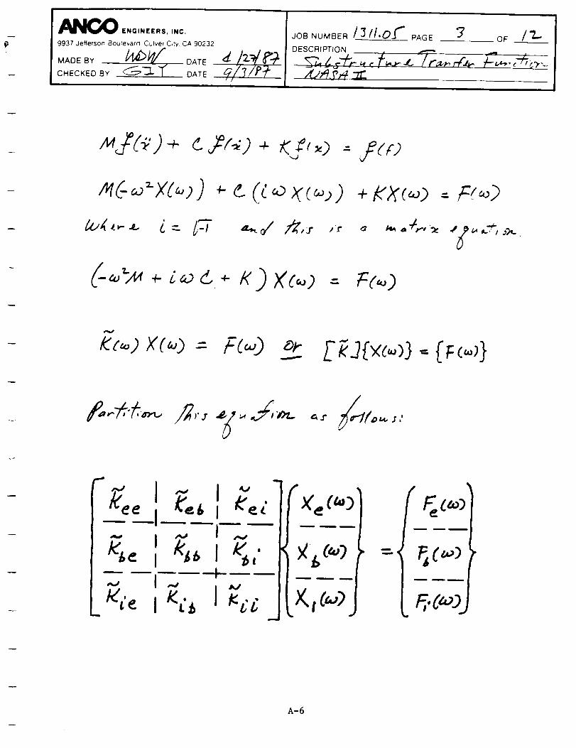
__E_O ENGINEERS, INC.
9937 Jefferson 8oulevarcl Culver C,tv CA 90232
MADE BY _//" -DATE
CHECKED BY _'_- "T _ , DATEf/
i
JoBNUMBER/ :_/I.07 PAGE _ OF / "7.-,,"
DESCRIPTION ,,,'T"',
,,,,'U_J',_ -rE
Le(
A-6
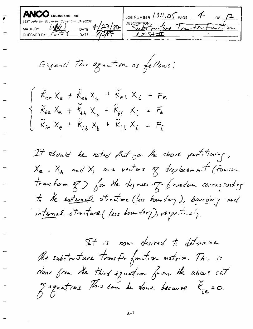
__O ENGINEERS, INC.
/-
J_o_.o,,_/3/'.of'_ .if-- o_DESCRIPTION, _ - ,...° _ _.
b
Kz_ Xe t- t<,csXs * KCc X i
- F_.
x'o ,
A-7
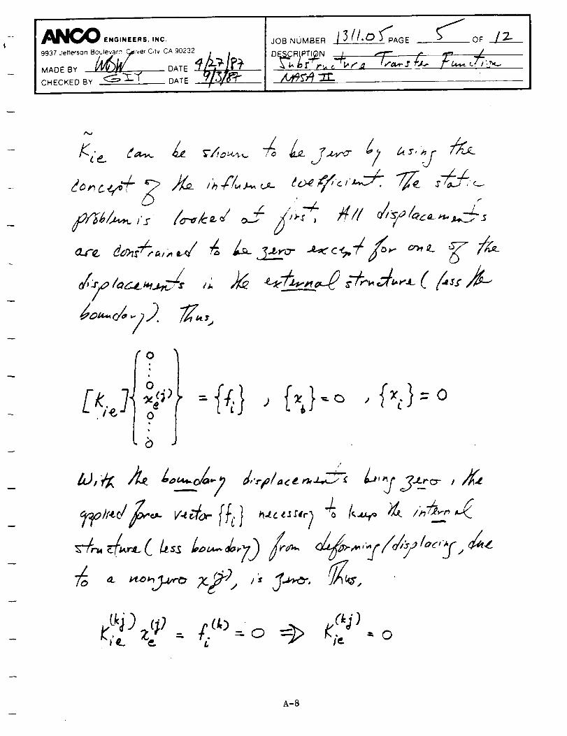
__tll_O ENGINEERS, INC.
9937 Jefferson 8oulevarct C,,mlver CAr CA 90232 . ,
CHECKED BY _____'Ty I_EE
JOBNOMSER I _ I/'O _'_PAGE _ OF
{'0
0 ,
04
4)
{(.},1..)-o.{_.}-o
k',,_ z,] -. _ : ,_ =O
&-8

_ ENGINEERS, INC.
9937 Jefferson Boulevard Culver C_tv CA 90232
C,ECKEOa¥- "_";'2_"f OATe
_zc_'_ _...Z ---
/l/,.)_Tn-r:'-,
(,_.)
/
•
o _i#
_,.,.'_<.__<_ _'-,- K_cx'i =
"'-I
-&-9
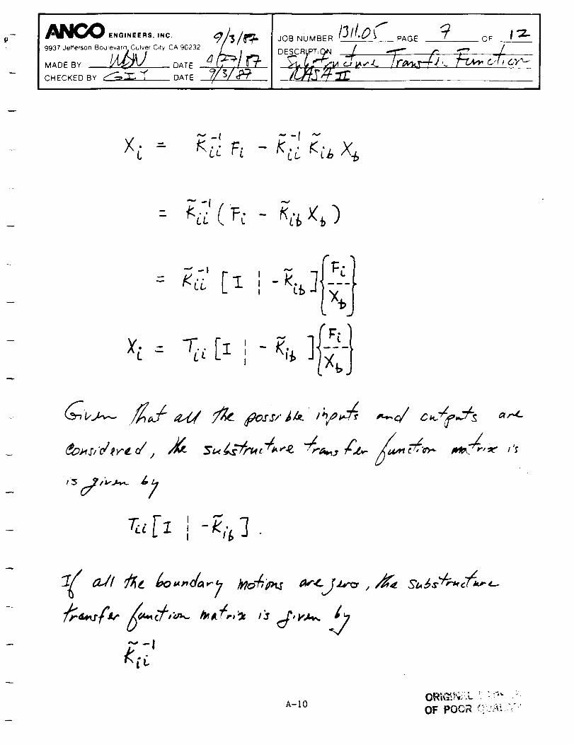
_ ,
- K_ _ X_
_ - __ [_ I - % ]Lx_j
t,:[z ,
A-IOOR,v,:.t,,_ ,,-
OF POOR <; ';_ ":"
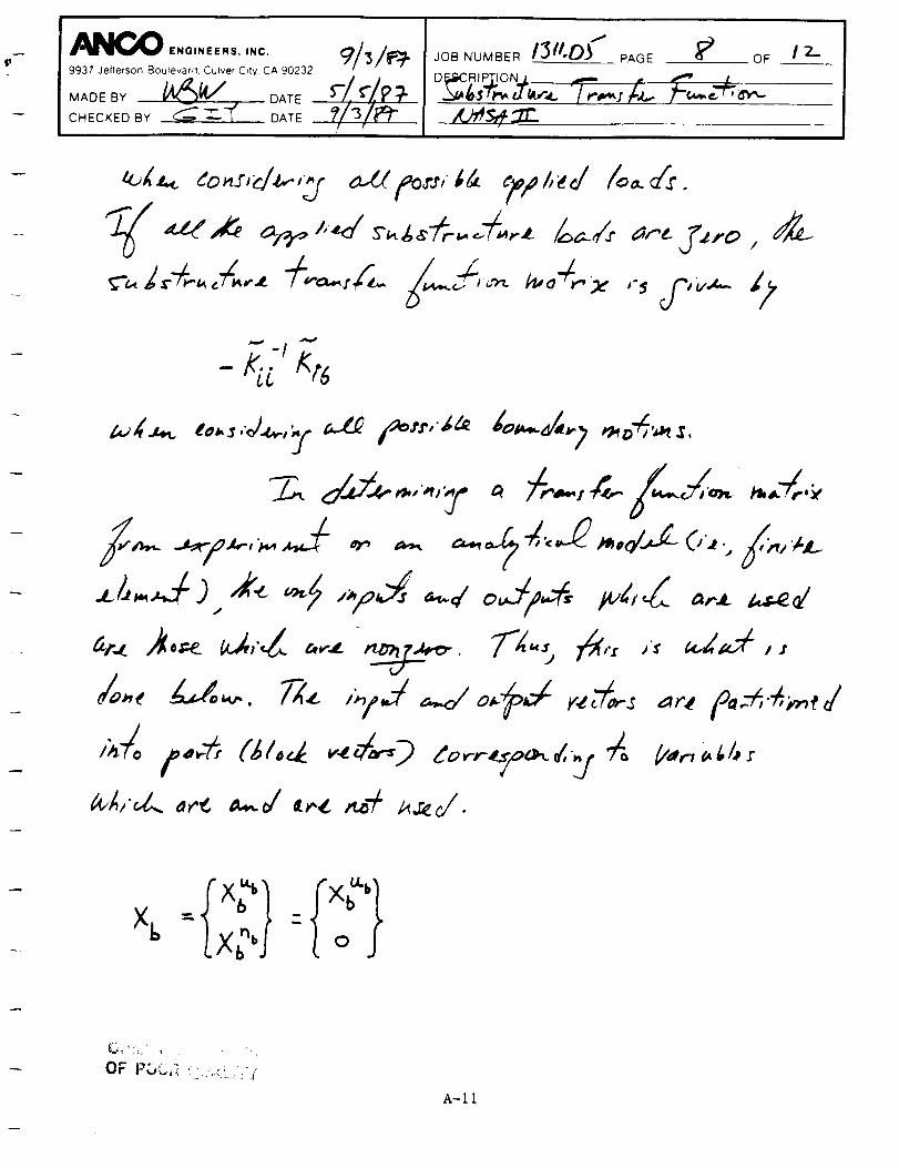
i_NC_ ENGINEERS, INC,
9937 Jefferson Boulevar_ Culver Crtv CA 90232
_,AoEB_ //_l¢/' °ATEc,EcKEDBY _" _'1" . DATE
_/_/_ JoB.u,,BE,_I:$11.0f",'AGE _ OF
,O,_s._,'tr_
12...
Ve,-,_ l li x
A-If

+'/l!OO _"°'"""''"° _>i_7_7;_o__ouT_,_,__;%___ DESCRIPTION . _ I, _ #"
/,.,'#_s.,,e:._
_,'<./.. c,_..z_</ _.,,.-d
A-t2

9937 Jefferson Boulel#r,_lve;C,lv CA 90232
MADE BY _V'L'_ _"V DATE
CHECKED BY _--_'-_-- "_ , DATE
f/,/n_/dr_
JoBNUMBER /3/I,° % PAGE lO OF / 2--D ESCJ=I I PTtOI_I ,'
X_ _
m
m
('T..__ TT..__
l LL LL.J
X( . - _L
X L = ILL 6.t,,
A-t3

li,
9937 Jefferson Boulevarn CuJver C_/v CA 90232 --
_o__ - _ _7 o_,__-I_Lr+CHECKED BY _ "_' DA_
JoB_U_BER1.7It.o_ .AGE I 1 OF I ""DESJ_,,EII PT IOJ_l • _ f _,
i,-.,[_ I -% 2I
A-14

993,Je,,e,so,._,o,,i_,_,,v_CHECKED BY -_"_ . DATE
I
JOB NUMBER t3 I I,_] PAGE t_ OF
#¢/'#ii_e-_l.-
,,," T,._+
Tii?+ _-'%"-/_i L _
i ~-I _T
A-I5

EIGENVALUES FOR SUBSTRUCTURE WITH CLAMPED (fixed) BOUNDARY
A-16

i__l_ ENGINEERS, INC.
9937 Jefferson Boulev_tq C__lver C,tv CA 90232/,,K/, 1
Y __ DATE
MADE BY
CHECKED 8 DATE
JOB NUMBER /3/'1.0 _ PAGE // OF
DESC..,_a_4;_ION _ .,_ . _ , . / /
A-t7 OR_G'!.N/'_,LF',:'.-:"_.-IT,
OF POOR QUA[..!';_I

,___ ENGINEERS, INC.
cHAEOEKBD9937JeffersOnByBoUle,_arcI.Culver_____-"_ C,tv CADATEDATE90232_ j.,_,/l ,,,_/0_,.
o
#4
miX i - F.,
JOB NOMBER / J/_ L_ _PAGE _ "_.OF
O FiSCAl PTIO,,N ,_ . _ . / /
-_4-_'c--,')o ,, "
,#Itw$.¢
[7;i]{#>}"o
A-18

K__O fNGINEEFIS, INC.
9937 Jefferson Bo/_le_ Cuiver Ci,v CA 90232
CHECKED BY _ "T" "_ DATE
JOB_UMSERf Jlt'O _'_AGE _ o_DES(_Ii_PTION j /2 -- _ , /
A-t9

SUBSTRUCTURETRANSFERFUNCTION--RELATIVERESPONSES
A-20

_ E"o'N""s,i"o.A
__o_ _oo,__c,_i_ /r.+7c.ECKEOBY_ _'f OATE .
_OB,OMS_,/'''/'°f._*_, / OF..__&DE__CRIPTION '_M X_"_/.._C_._/'_ '_1,_//.,'_._'_'
/u,4£,,#:Z_ /
A-2I
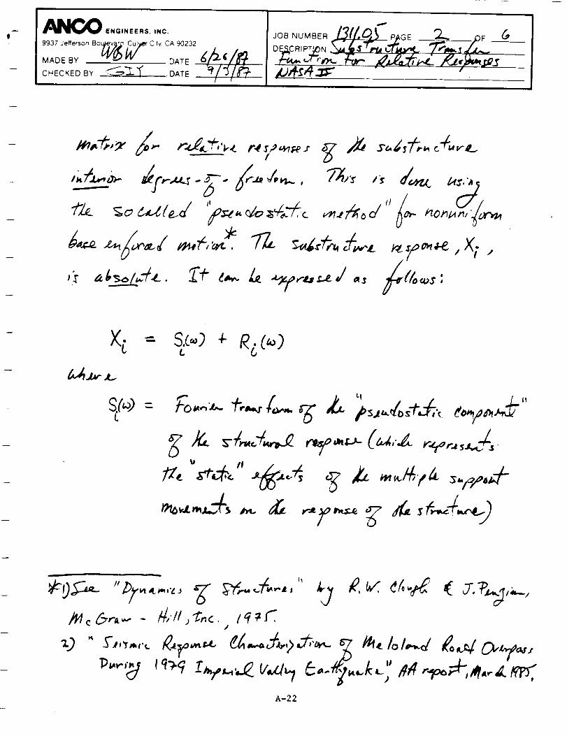
__°° =°___>_7"_"_o__
/_,@,_" 6_,- r_'_ r+_,_r+#,
tl II
#
A-22

_ ENGINEERS, INC.
9937 Jefferson Boulevard CulverC,lv CA 90232
JO=NoM=E=I3¢I.Od,GE "3
m
/
S_ is j,L..,.,,.. _,
5c - "P×_,
A-23
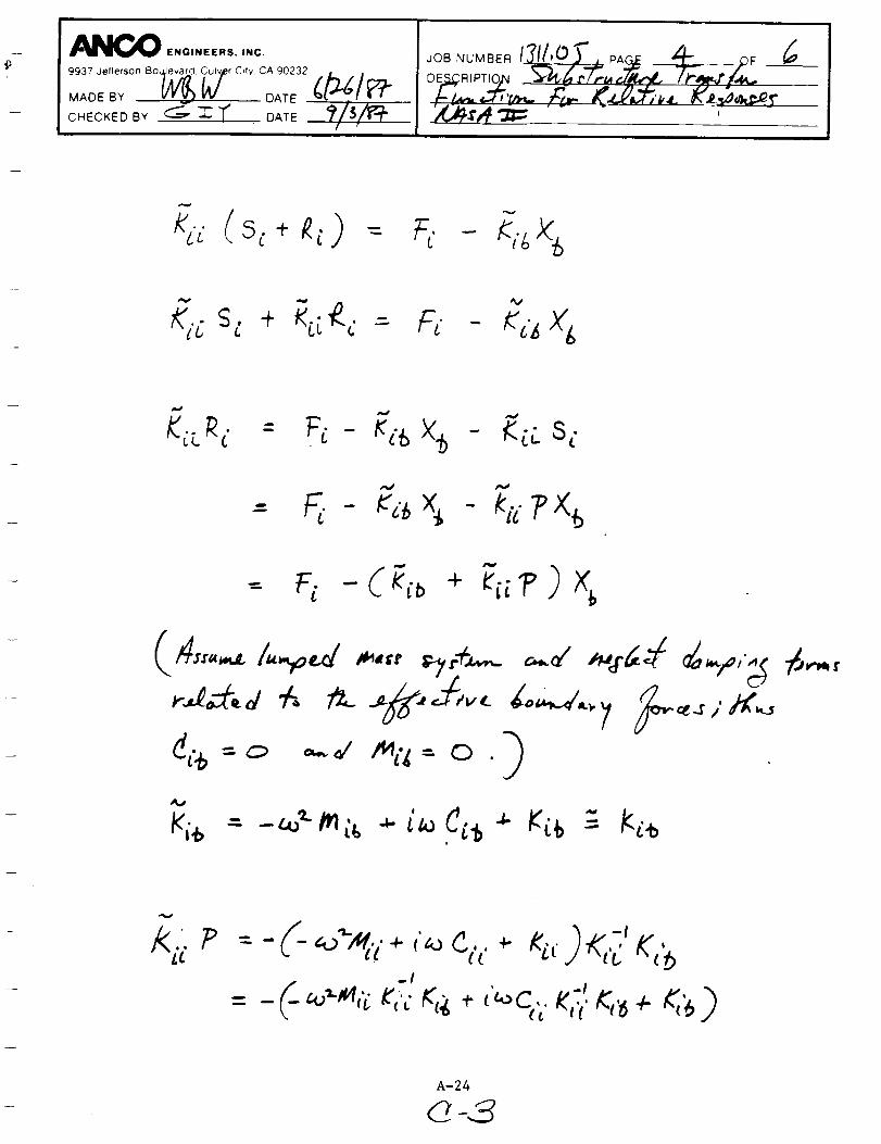
__O ENGINEERS, INC.
I
K_._4s__-_) - _:_.- C._z_
Im
I
-!
A-24

_ ENGINEEFIS, INC.
9937 Jefferson Boulevarn Quiver Cdv CA 90232
CHECKEOB',' _--_'_ _ OATE
:08::T_ERt__ _E _--O____ESC PTIQN _'L'_,I_" 1"14' t" _ '_'/'m_, I'/,,#,/l_'
e,,<_<= E
A-25

M__O ENGINEERS, INC.
CHECKEDBY _--------_'1" oArE
t
,d_,..__ rx_+S_
"Z-t-,J ipo,.,,'i z-,-, % <_6-I,,,,V
/"~ -I/-
: _,,W-,+ [- ,, '<,;'_,_J_<_J
..-(g<'<-'>: 4;" _,._<,'_+(-<_'',,'
I i _ _,,o .-- i II
A-26ORIGINAL 7': ,_- ,r,
OF POOR QU;;:LT/>_

DEFINING TWO DIFFERENT SUBSTRUCTURE INPUT
VECTORS CORRESPONDING TO THE BOUNDARY MOTIONS
A-27

_J_E_ ENGINEERS, INC.
9937 J elfers°n B°u'eD,_::Av CA 90232 /_/_.,_,MADE BY --- DATE 1_
CHECKED BY __ DATE 3_/! #i'_l,-_'.
°_o=.OM=E=/3{tOJ.AOE I O.___DESCRI!I,TJQNI x. _ _-xx>+._;'-_;;_L<'/,,,<t,,.,..
_.-_,);,:'t-= -
__/;,_,,_/- I_-
z=/M
"7",4#,,,,.p,_<Z"_'; ,o4
A-28
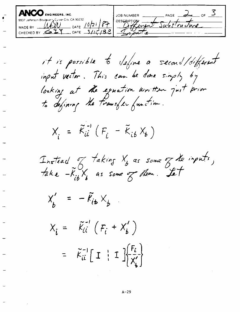
__III_ ENGINEERS, NC. k 2 2
7;017"'°i___"_021_CHECKED BY ___ DATE
-)JOB NUMBER E _,DESQI_I PT,O_ / PAG /" _ OF 3
/__306o..-_ Z. _.r7;,,,J_,.-__
- ( i;_ )x'. : _zi' r.- ×bt L
J
C=,+x;)mI
A-29

PAG E 3
9937 jefferson Bo_r C.tv CA 90232 ./t _1 I DES_I_IP ._ / /:_
CHECKED BY ___ DATE 3//_/_ _---'#1 _'_1;_ ,_,._ .-'_"l" ; " -
oF_5___
A-30

APPENDIX B
THEORETICAL BASIS OF MAC/RAN IV MULTI-INPUT
SINGLE-OUTPUT TRANSFER FUNCTION COMPUTATIONS

This ampendix contains a brief discussion o÷ some o÷ the themretical
aspects m+ the multi-input single-output trans÷er ÷unction computations
performed by MACIR_ IV [1,2]. The material is taken ÷rum Reference i.
A!so, some of the MAC/RAN LV input data listings tha_ were used to perform
this type oT computation is presented. Finally, a brief discussion o+ the
ANEO computer program/macro used to per+orm multi-input multi-output
Iransfer function computations, MIME), is presented.
References
I. _.K. Otnes and L. EnocRson_ "Digital Time Series Analysis," john
_iley and Sons, New York, New York, 1972.
2. '_MACIQAN IV, Time Series Data Analysis System, jJ University Software
Systems, E_ SegundoJ California, 1973.
B-2

THEORY OF MULTI-INPUT SINGLE-OUTPUT TRANSFER
FUNCTION COMPUTATIONS PERFORMED BY MAC/RAN IV
B-3

I
CHAPTER 9
TRANSFER FUNCTION AND COHERENCE
FUNCTION COMPUTATIONS
9.1 PROPERTIES OF FREQUENCY RESPONSE FUNCTIONS
A discussion of linear systems and the computation-
al procedures necessary for obtaining estimates of
them from measured time histories is presented in this
chapter. The simplest case, which has a single input
and a single output, is discussed first. A generali-
zation to the multiple-input, single-output system is
then presented. Computational requirements and proce-
dures for confidence limit evaluations are given in
Sections 9.4 to 9.9. Extensions to other ideas of
multivariate statistics are given in Section 9.10.
v
If
J4
9.3 SPECTRAL RELATIONSHIPS FOR MULTIPLE-INPUT LINEAR
SYSTEMS
A model of a linear system responding to multiple
inputs will now be considered. It will be assumed that
MULTIPLE-INPUT LINEAR SYSTEMS 333
p inputs exist, and a single output is measured. Three
types of coherence functions, ordinary, multiple, and
partial, play an important role in this analysis, and
their evaluation is discussed.
Consider a linear system with time-invariant param-
eters and p inputs x£(t), £ = 1,2 ..... p. That is
y(t) = £ y£(t) (9.21)

where y£(t) is defined as that part of the output pro-
duced by the ith input, x£(t), when all the other in-
puts are zero (see Figure 9.2). The function h£y in
Figure 9.2 is defined as the weighting function asso-
ciated with the linear system between the input xz(t)
and the partial output y£(t). Hence, y£(t) is givenas follows:
yz(t) = ___ h£y(T)xz(t- T)dT(9.22)
The Fourier transform of (9.22) gives
Yz(f) = H£y(f) Xz(f)(9.23)
where Y (f) and X (f) are the Fourier transforms of
Y (t) and x (t), respectively. Then the Fourier trans-
form Y(f) for the total output is
P P
Y(f) = _ Y£(f)= _ H£y(f)X£(f) (9.24)£=i £=i
The statistician reading this material should immedi-
ately note that (9.24) is a regression equation for
zero mean variables. The dependent variable is Y, the
independent variables are X£, and the regression coef-
ficients are H£y. Thus, electrical or mechanical en-
gineering frequency domain transfer function concepts
334 TRANSFER AND COHERENCE FUNCTION COMPUTATIONS
can be interpreted by the statistician via regression
analysis of complex random variables. This concept is
delved into in considerable detail by (Akaike, 1965).
The gist of it is that we can treat each frequency
band independently, and by accomplishing many complex
variable regression analyses (one for each frequency
band) we will obtain the entire frequency domain
functions.
B-5
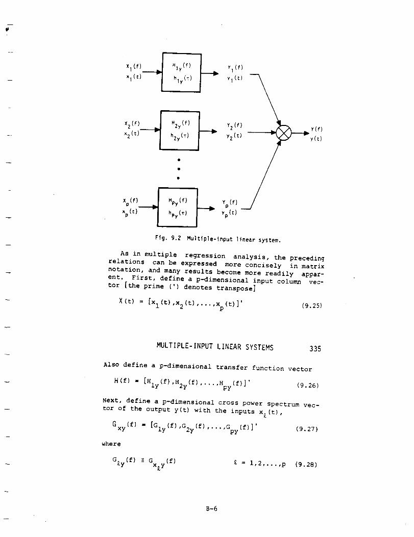
Hpy(f)
hpy(T)
Y_(F)
Y2 (f)
yz(t)
Yp(f) __/
yp(t)
Fig. 9.2 Multiple-inputlinearsystem.
Y(f)
As in multiple regression analysis, the preceding
relations can be expressed more concisely in matrix
notation, and many results become more readily appar-
ent. First, define a p-dimensional input column vec-
tor [the prime (') denotes transpose]
X (t) = [Xl(t),X2(t), .... Xp(t)]'(9.25)
MULTIPLE-INPUT LINEAR SYSTEMS 335
Also define a p-dimensional transfer function vector
H (f) = _[Hly(f),H2y(f) ..... Hpy(f)]' (9.26)
Next, define a p-dimensional cross power spectrum vec-
tor of the output y(t) with the inputs xi(t),
Gxy(f) = [Gly(f) ,G2y(f) ,... ,Gpy(f)] ' (9.27)
where
G_y(f) _ Gx_y
(f) £ = 1,2 .... ,p (9.287
B-6

Finally, define the (p x p) matrix of the
cross spectra of all the inputs x[(t) by
B
Gll(f) Gl2(f) ... Glp(f)
Gxx (f) =
G21(f) G22(f) ... G2p(f)
Gpl (f) Gp2 (f) • •. G (f)PP
power and
(9.29)
where for simplicity we adopt the notation
Gij (f) = Gx.x. (f) i,j = 1,2 ....• p (9.30)x 3
The matrix Gxx(f) is Hermitian, since it equals its
conjugate transpose. This implies, for example, that
the eigenvalues of Gxx(f) are real numbers, should
these parameters be of interest in an application.
The system of linear equations to obtain a least
squares solution for the H£y(f) of (9.23) is the ma-trix equation
336 TRANSFER AND COHERENCE FUNCTION COMPUTATIONS
G (f) = G (f) H(f)xy xx
(9.31)
This is equivalent to
"Gly (f)"
G2y (f)
Gpy (f)
Gll (f) G12 (f)
G21 (f) G22 (f)
GpI (f) Gp2 (f)
... Glp (f)
... G2p (f)
°.. G
PP
"Hly (f)"
H2y (f)
(f) Hpy (f)9
(9.32)
The solution to this system of equations is
H(f) = G-l(f) (f)xx Gxy [9.33)
For the practical situation, we estimate the spectra
and cross spectra in (9.32) with the procedures de-
scribed in Chapters 6, 7, and 8.
B-7

EXAMPLE OF MAC/RAN IV MULTI-INPUT SINGLE-OUTPUT TRANSFER
FUNCTION COMPUTATION INPUT DATA CARD IMAGE LISTINGS
B-8

RELATIVEMODULETRANSFERFUNCTIONMATRIXCOMPUTATIONUSINGPSDANDTRANSPROCESSORSIN MAC/RANIV
B-9

JBHEAD REL.SIMP.TRANS.FUNCT.- PSD,J4F457U ACC(4MODES-2MODES),F6=OFILIN J4F457U2.SDF
C* ACCEL. RESP.S
FILIN CCHAN
C* ACCEL. RESP. S
FILIN CCHAN
FILIN J4F457U4.SDF
C* ACCEL. RESP. S
FILIN CCHAN
FILIN RANTRNCI.SDF
C* APPL. FORCES
FILIN CCHAN
PREP
PREP SRCE RF'SD-SISO,PREP TYF'EJ4F457URTF60
PLUG
PLUG WIRE TIME, SEC.PLUG SUB RELACC5
PLUG WIRE RELACC5
PLUG WIRE ABSACC4
F'LUG WIRE ABSACC7
PLUG MULC F5X50.
PLUG WIRE FORCEF5
PLOT PLOT
PLOT SCALE
FILOUT RELPSDA5.SDF
PSD TRANS
PSD TOUTMTFC
F'SD RETAIN
PSD F'OUT33333
F'SD PLOT
F'SD SCALPSD
PSD SCALCSD
PSD SCALCOH
PSD SCALTFF
FILIN J4F457U2.SDF
C* ACCEL. RESF'.S
FILIN CCHAN
C* ACCEL. RESF.S
FILIN CCHAN
FILIN J4F457U4. SDF
C* ACCEL. RESP.S
FILIN CCHAN
FILIN RANTRNC1.SDF
C* APPL. FORCES
FILIN CCHAN
PREP
PREP
PREP
PLUG
PLUG
PLUG
F'LUG
PLUG
PLUG
PLUG
SRCE RPSD-SISO,TYPEJ4F457URTF60
WIRE TIME, SEC.SUB RELACC6
WIRE RELACC6
WIRE ABSACC4
WIRE ABSACC7
MULC F5X50.
TIME A4(IN1) A5(OUTI> A6<OUT2)
i. 2. 3. 4.
A7(IN2)
5.
A4(IN1) A5(OUTI> A6(OUT2) A7(IN2)
o 3 4_m • • -i
F5
1
O. 0
1024.0
0.0
i 1
7 3
-2 2
2 3
5 4
I0 -I0 50.
-I0 5
24.0
6.0
-2
0. 12
O. 0
O. 0
0.0
O. 0
TIME
I.
A7 (IN2)
5.
A4(IN1)
2.
F5
2.
8.0
8.0
8. (')
8.0
A4(IN1)
2.
A5 (OUT I )
3.
0.0
A5(OUT1)
3.
A6 (OUT2)
4.
I00.
A6 (OUT2)
4.
A7(IN2)
5.
1
8
2
5
10
1
4
2
:3
4
-I0 50.
-2
B-IO

PLUGPLOTPLOTFILOUTPSDPSDPSDPSDPSDPSDPSDPSDPSDEND
WIRE FORCEF5PLOTSCALERELPSDA6.SDFTRANSTOUTMTFCRETAINPOUT33353PLOTSCALF'SDSCALCSDSCALCOHSCALTFF
0.0
I 024.0
0. o
O.00.0O.00.0
-i0
24.0
8.08.08.08.0
5
6.0
0.0
0. 12
1O0.
B-If

JBHEADREL.MISO TRANS.FUNCT.FROMTRANS, J4F2F_ ACC(DIS4-DIS2)MODES, F3=OFILIN RELF'SDA5.SDF
FILOUT JUN_<RA5. SDF
TRANS TAPE
FILIN RELPSDAb. SDF
FILOUT JUNKRAb. SDF
TRANS TAPE
END
B-12

ABSOLUTEMODULETRANSFERFUNCTIONMATRIXCOMPUTATIONUSINGPSDANDTRANSPROCESSORSIN MAC/RANIV
B-13

I ]BHEAD SIMPLE TRANSFER FUNCTION
FILIN J4F470U4.SDF
C* ACCEL. RESF'.S TIME
FILIN CCHAN I.
C* ACCEL. RESP. S A7(IN2)
FILIN CCHAN 5.
FILIN RANTRNC1.SDF
C* APPL. FORCES F5
FILIN CCHAN 2.
PREP
PREP SRCE APSD-SISO,
PREP TYPEJ4F470U4F60
PLUG
PLUG WIRE TIME, SEC.PLUG WIRE ABSACC5
C*FLUG WIRE ABSACC4
C'PLUG WIRE ABSACC7
PLUG MULC F5X50.
PLUG WIRE FORCEF5
PLOT PLOT
PLOT SCALE
FILOUT ABSPSDA5.SDF
PSD TRANS
PSD TOUTMTFC
PSD RETAIN
PSD POUT33333
PSD PLOT
PSD SCALPSD
PSD SCALCSD
PSD SCALCOH
PSD SCALTFF
FILIN J4F470U4.SDF
C* ACCEL. RESP.S
FILIN CCHAN
C* ACCEL. RESP. S
FILIN CCHAN
FILIN RANTRNCI.SDF
C* APPL. FORCES
FILIN CCHAN
PREP
PREP SRCE APSD-SISO,PREP TYPEJ4F470U4F60
PLUG
PLUG WIRE TIME, SEC.
PLUG WIRE ABSACC6
C*F'LUG WIRE ABSACC4
C'PLUG WIRE ABSACC7
PLUG MULC F5X50.
PLUG WIRE FORCEF5
PLOT PLOT
PLOT SCALE
FILOUT ABSPSDAb. SDF
PSD TRANS
PSD TOUTMTFC
F SD RETAIN
PSD POUT33333
FROM PSD,J4F470U4 MODEL
A4(INI) A5(OUTI)
2. 3.
1 1
3 2
o 3
5 4
6 -6 50.0(')
-6 3
RANTR IN. ,
A6 (OUT2)
4.
0.0 24.0
1024.0 6.0
0.0
O. 0 8.0O, 0 8.0
0.0 8.0
0, 0 8.0 0.0
TIME A4 (IN1 ) A5 (OUT1)
I. 2. 3.
A7 (IN2)
5.
F5
2.
0.0
1024.0
O. 0
0.12
.06
A6(OUT2>
4.
1
4
1
2
2 3
5 4
6 --6 50.00
-6 3
24.0
6.0 O. 12
F6=O
B-14

F'SDPSDPSDPSDPSDEND
PLOTSCALF'SDSCALCSDSCALCOHSCALTFF
0.00.00.00.0
8. ()
8.0
8.0
8.0
B-15
c).0 • 06

f
JBHEAD MIMO TRANSFER FUNCTION FROM TRANS, ,38F5F6 MODEL RANTR IN., F6=0FILIN ABSPSDA5. SDF
FILOUT OUNKAA5.SDF
TRANS TAPE
FILIN ABSPSDA6. SDF
FII_OUT JUNKAA6.SDF
TRANS TAPE
END
B-16

BRIEFDISCUSSIONOFANCOCOMPUTERCODEMIMOFORCOMPUTINGMULTI-INPUTMULTI-OUTPUTTRANSFER
FUNCTIONSUSINGMAC/RANIV
B-17
USE OF THE TRANS PROCESSOR AND
VERIFICATION OF TRANSFER FUNCTIONS
June 1987
ANCO Contraot No. 1311.05C (NASA}
P.O. No. 2461
Prepared for
ANCO ENGINEERS, INC.
9937 Jefferson Blvd.
Culver City, California 90232
Prepared by
UNIVERSITY SOFTWARE SYSTEMS
E1 Segundo, California
B-18

J
3
4
Table of Contents
OVERVIEW OF WORK DONE .................................. 1
COMPUTING AUTO AND CROSS SPECTRA ....................... 1
2.1 Degrees of Freedom ................................. 1
2.2 Segmentation ....................................... 2
2.3 Distinction Between Effective Resolution Bandwidth
and Computational Bandwidth, and the RETAIN Option ..... 2
THE LINEAR SYSTEMS PROCESSOR (TRANS) ................... 3
3.1 Spectral Matrix Prepared by PSD .................... 3
3.2 Ordinary, Multiple, and Partial Coherence .......... 3
COMPUTATION PROCEDURE SUMMARY .......................... 44.1 ANCO's Automatic Control File Generator ............ 4
4.1.1 Adjustable RETAIN Option ...................... 4
4.1.2 Using TRANS for Plotting ...................... 44.1.3 Confidence Limits ............................. 5
4.1.4 Frequency Bounds, and Instabilities in
Computations ........................................ 54.2 Plotted and Printed Results ........................ 5
i
B-19

!
1 OVERVIEW OF WORK DONE
The primary task of this job was to confirm the automatic control
file generation for Micro-MAC/RAN and Micro-MAC/RAN:TRANS
processing of finite element model results. The basic problem
was to isolate a linear substructure from the finite element
model and simulate a multi input / multi output linear system
whose transfer functions could be effectively computed by a
combination of the MAC/RAN PSD and TRANS processors. The two
endpoints of the substructure were treated as the input points
and the interior nodes the outputs. Transfer functions were
computed between all input/output pairs, but not between outputs
or between inputs. Two cases were processed by ANCO. Each case
used a different base excitation for the large model, therefore
the resulting endpoints of the substructure were different.
Additionally, the first case processed 4095 data points with a 50
sps sampling rate, while the second case processed 1024 points
with a 16.667 sps sampling rate. USS was to duplicate ANCO's
results if possible, and to make recommendations on the
procedures used to obtain these results. In particular, to
determine whether the automatic control file generator was
setting up the proper control file for MAC/RAN. In making these
Conclusions, various procedural issues were discussed. The
following sections briefly describe these issues. The last
section makes some recommendations as to control procedures.
2 COMPUTING AUTO AND CROSS SPECTRA
2.1 Degrees of Freedom
The PSD processor uses a technique that combines segment and
frequency averaging to obtain statistically meaningful auto
and cross spectra. By statistically meaningful, we mean that
the resultant spectra has enough degrees of freedom (d.o.f.)
to be considered a reasonable expectation of the mean power
present in the data, as a function of frequency. By
definition, the d.o.f, in a spectrum computation is
2BN
/,
where
B is the bandwidth
N is the number of points
/. is the sampling rate
If the data is too large to fit in core as one segment, we
need to distinguish between the number of points per segment,
N, and the number of points, N.
1
B-20

I
By default, PSD will try to make the proper decisions for what
segment length the data needs to be broken down into and the
number of frequency averages necessary to achieve a default
d.o.f, of 30. This happens when the user leaves the field for
Bandwidth on the first PSD controller blank or zero.
If PSD has enough core memory available, it will try to
process data as one segment, and do frequency wise averagingto obtain the desired d.o.f.
In this case, the bandwidth becomes
151,
N,
2.2 Segmentation
If PSD does not have enough memory to process the data as one
segment, it breaks the data down into the minimum number of
equal length segments that will fit into available memory.
Zeros are padded to achieve a transformable length. Since
segments will be averaged, if the bandwidth of each segment is
S., then the d.o.f, will be
2N 15I,n = _30x(the number of segments)
f, N,
If we had left the Bandwidth field blank or equal to zero,
then PSD would need to modify the bandwidth for each segment
to achieve the proper d.o.f, after averaging the segments.
Also, if trailing zeros were padded in the segment(s), a
weighting factor is used to compensate for the diminished
magnitude of each segments Fourier transform. Refer to the
MAC/RAN Reference Manual, Chapter 8 (D.3)
2.3 Distinction Between Effective Resolution Bandwidth and
Computational Bandwidth, and the RETAIN Option.
Generally, if points of a spectral function are computed at
the Effective Resolution Bandwidth, then the spectral values
are approximately statistically independent. If a finer
spacing is used, by way of PSD's RETAIN option, more points
will be computed, however with little if any statistical
significance. That is, there will be overlap between the
estimates computed.
If more points are desired, to match with other functions, or
for finer resolution of plots, then making the computationalbandwidth smaller than the resolution bandwidth will achieve
this at the expense of increased computation time and larger
listings and plot files. By default, PSD tries to use a
computation bandwidth equal to the desired resolution
bandwidth, since that is the minimum spacing that gives
B-21

w
i
approximately non-overlapping, independent frequency values.
This is also directly related to the d.o.f, in the
computation. That is, if a very few d.o.f, are selected
because the user specified a very narrow resolution bandwidth,
then the frequency values will not be at all orthogonal, since
the variance in each estimate would be very high (little or no
frequency averaging was done).
3 THE LINEAR SYSTEMS PROCESSOR (TRANS)
3.1 Spectral Matrix Prepared by PSD
A PSD option is to create a spectral matrix for the TRANS
processor using the aforementioned techniques. This matrix
contains the auto spectra of the output and all inputs, plus
the cross spectra between inputs and output and the cross
spectra between all pairs of inputs. This is because TRANS
will try to determine the effect of each input on the output_
composite response, so that individual transfer functions can
be computed that "subtract out" the effects of the inputs that
are not involved in the path for the particular transfer
function. This concept is tied directly with the three types
of coherence that are computed.
3.2 Ordinary, Multiple, and Partial Coherence
The idea of coherence is directly related to the linearity of
the considered system or systems. TRANS computes the three
coherencies automatically. The ordinary coherence is also
computed by PSD but for a multiple input system, it is useful
primarily for comparison purposes with the partial coherence.
It is, however, the only coherence computed between inputs, as
the inputs are assumed to be independent of each other. (Note
that this does not mean they need be statistically
independent; only that we assume they will "move" in the same
way regardless of how many of them are present or where they
are in the system. They are the "givens" in our set of
equations). TRANS computes ordinary coherence between input
pairs as an option, and we do not need this option for the
problem considered here, since we know that the inputs to the
substructure are really responses due to a base motion in the
global system.
The partial coherence tells us how much of the computed
response is due to a particular input. That is, if input 7
has a strong effect on output 5 and input 4 has a secondary
effect on output 5, the partial coherence between 7 and 5
should be close to 1.0 since the response is almost completely
due to the input at 7. Similarly, the partial coherence
between 4 and 5 would be low, as the response at 5 would
"feel" a strong presence from another point in the structure,
namely input 7. The ordinary coherence ignores any distinc-
B-22

tion between other inputs and the input used in the
computation. It does not condition the coherence computation
on any other input. Thus, the ordinary coherence between 7
and 5, for example, might be high if the effect of 4 and other
inputs is relatively minor. If multiple inputs contribute
equally to an output motion, the ordinary coherence
computation is usually off the mark, as it senses what itconsiders to be non-linearities in the transfer function.
That is, there are unaccountable components in the response
given the information that the ordinary coherence has to make
its computation.
The multiple coherence plays the part of the ordinary
coherence for a multi input system. It assumes that it has
the information from all the inputs considered and computes a
composite coherence. For linear systems with known inputs and
low noise, the multiple coherence function is usually very
close to 1.0 across the spectrum. If there is a drop in
multiple coherence, this is an indication that a source of
motion has been ignored, or that noise was introduced
(incoherent components), or that the system is in fact
somewhat nonlinear.
4 COMPUTATION PROCEDURE SUMMARY
4.1 ANCO'S Automatic Control File Generator
USS's replication of the preliminary ANCO computations show
that the automatic control file generator computed a good set
of instructions for the PSD and TRANS processors. However,certain recommendations are made. These are:
4.1.1 Adjustable RETAIN Option
In light of the above discussion (Section 2), USS recommends
that the automatic generation program allows the RETAIN
decimation factor to be entered as a variable, since blindly
retaining all points can be misleading as well as highly
costly for large or many computations.
4.1.2 Using TRANS for Plotting
ANCO writes a Standard Data File (SDF) of the real and
imaginary parts of the computed transfer functions using the
TRANS TAPE option. They then use the PLUG and PLOT
processors to plot the magnitude and phase of these transfer
functions. TRANS directly plots the transfer functions
along with the various coherence functions. USS matched the
ANCO plots using only the TRANS processor. This eliminated
some computation time and complexity that are introduced by
the PLUG and PLOT processes. Additionally, the coherence
functions should not be ignored, since for production runs,
4
B-23

they will verify that the transfer functions are meaningful.
The concepts of coherence are directly related to multiple
input transfer functions due to their statistical nature.
4.1.3 Confidence Limits
Another reminder of the statistical nature of spectrum
computations is that upper and lower bounds are printed and
optionally overlayed on the TRANS plots. USS recommends
that this concept is noted, even if confidence limits are
not plotted during the course of the production runs. By
default, TRANS computes response functions with a 95%
confidence that the results are between the upper and lowerconfidence levels. Note that if the difference between the
upper and lower confidence levels is very large compared to
the magnitude of the 95% value computed, then the transfer
function may still be suspect. (For example, being 95%certain that the actual transfer function lies between 0 and
infinity is quite meaningless).
4.1.4 Frequency Bounds, and Instabilities in Computations
A new TRANS controller allows printing and plotting of
results between frequency start and stop values. This is
useful if there is a problem computing the inverse of the
spectral matrix or computation of transfer functions by
dividing two statistically insignificant values, e.g. noise
into noise when very little energy is present in the input
or output in a frequency range. Also, for situations where
a great deal of oversampling was done in the time histories,
one does not want to deal with values of response or
coherence well above a frequency where energy is known not
to exist in appreciable amount. The TRANS FREQ and TRANS
SCAL controllers allow plotting of the points of interest
without spikes or glitches due to the aforementioned
phenomena. The TRANS listing file will inform the user if
there were any instabilities in the computation and at what
frequencies they occurred.
4.2 Plotted and Printed Results
Delivered with this report are two sets of plots and listings
that illustrate the matching of ANCO's results by USS. The
first set (Set i) corresond to phase 1 of the test runs and
are designated by Source and Type annotation "COSMOS/M NASA
1311.0." Set 2 is annotated "NASA PHASE II" and corresponds
to phase 2 of the test runs.
Note that the PSD plot and print suppress option was invoked
to eliminate the display of unwanted information (TRANS will
provide the relevant plots and print in the second step),
however, on occasion it is instructive to view the spectra of
the inputs and the outputs from PSD to see where the greater
5
B-24

part of energy lies in the spectrum, and to get an idea aboutthe signal to noise ratio in the transfer functioncomputations.
B-25
'W
WO0Z
.JLUZZ
IU
n-Ob.
Z0
Z
LL
W
Z0O_
LUnr
>-CJZW
W
0
fqO_l.CJ
0"1
Z U
UJ>iii
Z_J
_r7OH
tnZO0r.JU
U')
WC_0Z
II
I-
I--
0
I I i I L .... i
I !' i i
0
OT
0
0
UO±3V NIV9
0
Lo
0
p-,
0
N0
Z[d
C_LU
o 0[
m Lu
0
0
0
OJ
B-26
-7
I IO
lioLOO_t_
!_o,,,O
IIZ
LUOOZ
_JLUZZ
it(.2Z
t.L
tOU_ZOO-COLiJrr
>-OZLU
C_LIJrrb_
_JW II
Ill5"._I
f._ 0 I-
_E l.I_O.
omz_-O_(..1f_) 0
0
0
I
0
0
01;
! I i
0
0
I I I
0 0 0
0 0 0
I I I
(030/ 3SVHd
IILI
O
O
I
O
0O
O
O
O
CD
O
Cq
O
OJ
O
O
O
N_b
>-UZLU
0LUrrLL
B-27

WO"OZJWZZ7-CD
n-O11.
Z0
CDZ
W
Z0O.
Wn_
>-UZ
Z;
n_b_
0
_4_O.,-41.0
-_OWO_ Q
ZlIZ.JUJ II
UJ__J
0_D_
_Z_-
(DCDO
I I I | li
0 0 0 0 0• 0 O
0 I.n 0 I1") 0_ _ '_ ',4 I._ 0
_m01; UO.LOV-I NIV9
B-28

f_
W
Z
d
"1"_J
n-Ob-
Z0I-Il--(.JZ
_,L
Wf_Z0n
IiIC£
UZ_J
C_111
b_
0
COO_t,q
._owffl 0
ZlIZ._1W_>m
IE.-I
(/] D I--
IE tl_ _mZI--O0_LJ L._O
0
00
I
0
00
0
I I
0
0
!
C 3C::3)
b
00
I
3SVHd
b
0
I
B-29
O
(3l
h.
0
00CUI
N]l
ZW
0W
o n"LL
0
0i
0
0
!
0
(21o3
!
0
I_r'l
! J ! !
0_
[ i [
0 0 0
0 I£1 0
IdOlgV--I NTV9
B-30
O
O
O3
O
I°
O
O
O
Lq
O
O
O3
O
C0
O
O
O
NT
>-
ZLd
LO£CLL

I
0
"_l.n
Q
ZIIZ.dILl II
I.LI_-..J
.f.n o I-
_-_n_" f.r} Z I--
ILl UUOQ0Z
.JWZ:7
-1-U
rr(3LL
Z0
UZ
.:3LL
UJU3Z0nLrJLLIrr
>-UZIii7E_LU
LL
I
<
0 00
0 0OJ _-4 0
I I I
/
I
/f
'O
O
I".-
O
(/3
o 1Nq.-.
1.13 "---"
O
O
O
• ('M
O
O
m r u O
0 0 0 0
0 0 0 0
l I I I
(03G) qSVHd
>-.
ZLLI
LLiITLL
B-3I

WQQZ_JZZICJrr0b.
ZQ
b-(JZ
LU
Zon_OWrr
>-CJZW
C_LUrrtu
0
000
tO 0
Z IIZJ111 II>LW
U_ 0 I.-
gl Z l--
f.._U 0
0
_O
I ! I
I I J i
0 0 o o
UO/OV NIVO
0
B-32
0
0
0
LO
0
0
0
01
0
OJ
0
0
0
0
0
N7-
>..[_,1ZILl
C_LUrr"L:_

, t_ I |
t b b
0
I
00
0 0 0
0 I I
(930) 3SVHd
Fir
0
0
U_
N0
g°_
0
0
i
0
_.o00_dI
B-33

,q.
LU[]0Z
(.If.J<
JWZZ<7-CJ
n-O11.
Z0I--4i--UZ
LL
l.IJU]Z013.O3LUrr
>-UZLUZ)(3LUrrb_
Lr)
OW_C_010
.Z0
CJH r.jMII<
LIJ IIUJ>O'JUJ<.JI-
H_
ffl Z t---
ZUQ
0
0rrl
!
0
t_
01;
I
0
0
! !
0 0
UOLOV9 NIV@
I
O O
O
O
CO
O
h_
O
o N7-
Lr)
• U_" Z
III
(ZlIii
o A"m Iw.
0
0
0
0
B-34

P
Wr70Z
! !
0 0 00
0 0 0tO _" Od O
! !
I !
0 0
0 0
I I
3SVHd
0
0tOI
0
GO
0
0
U3
o NI
o >-• 0
ZLU
LUom
0
0
0
0
B-35

00
I I I I
I
0
LOC_
| i' I I
O_
0 0 0
WOZSV_ NIV9
0
L_
0
0
0
0
o_
0
.t't/
0
0
0
B-36

i
Wn0Z
_D
dWZZ"l-
n-Ob_
Z0
UZ
LL
ILlO_ZOnO_UJrr
>-(.2ZUJ_D
UJrrb_
OLULOrnOlO'Z
0
_JLU II
I_3>OOU3
"I-CL r_ _-
_b_nO_Z_-
ZUO
0
00m-4
i
0
0Ln
/
I I I ,
0
0
' b b0
0 0
I I I
(9:90) EtSVHd
0
138
0
r.:
O
o%
0
0
0
0
00(M
I
B-37

LUO0Z
(JU
JUJZZ
7-U
rr0b_
Z0I-'4
UZ
b_
LU01Z0O_or}IJJn"
>-UZW
C_UJri-ll.
l--I
UJO_
7-13.
O_
Z
0
(D
tO
oW_C30_C3.Z
o
U
_JUJ II>tO..J
C3_-
b_nZ_
(JO
I I I I I
I I I I I
0
L_
0
_7
0 0
m
UOIOV9 NIV9
0
B-38
0
0
0
0
p,.
0
LO
o N
_" ZLU
C_LU
o n-_n b_
0
0
0
0
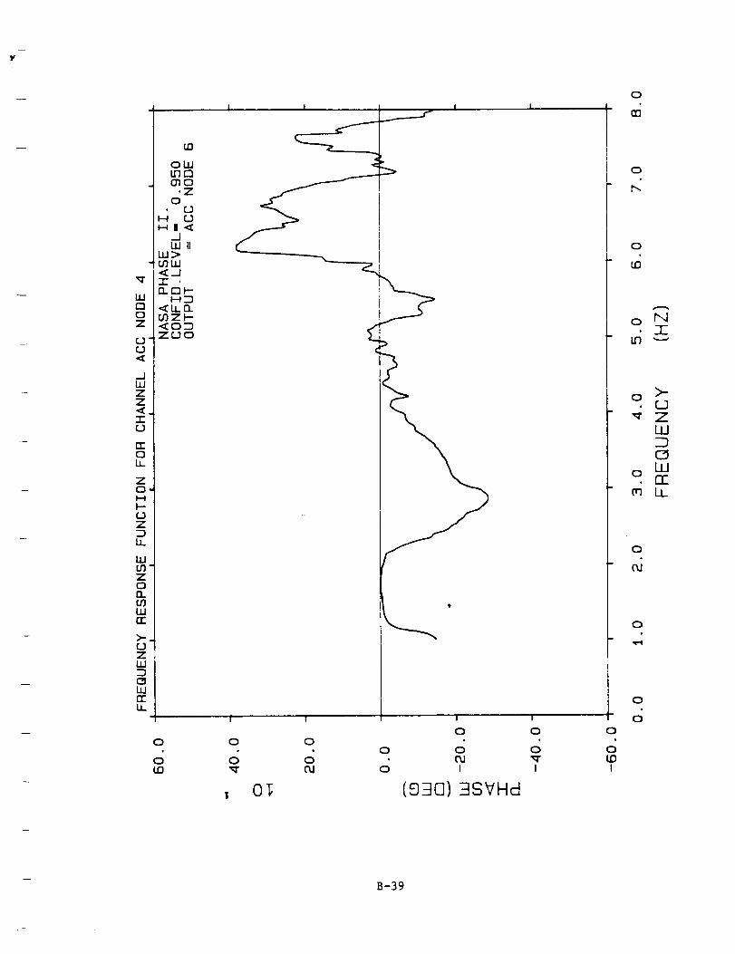
tlJOOZ
cJcJ
.JlIJZZ
7-U
n-Ob_
ZOH
H-(JZ
U.
I.U0_ZOnO_Wrr
UZtU"7OtUrrtu
ED
0111L0r7010"Z
0U
H U
IUJ II
W>O_LIJ<l7-nc]h-
<LLnO_Z_--"_0_Z_O
0
0tO
I
0
0
f
!
0
0Od
!
0
0
!
0
0
I
3SVHd
I
0
0
I
0
iQB
o
h.
0
0
0
0
0
0
0
0
0
0
I
hqI
>-(DZLU
C_LU0Ch
B-39
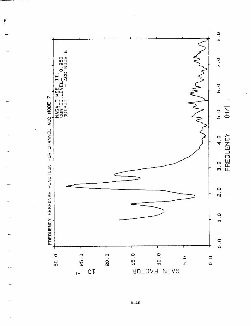
h,
WO0Z
{j-U
dUJZZ
7"U
0b_
Z0
UZ
U-
W03Z0O.01UJn-
>-UZ
C3UJrrb_
OWLOt7010
.Z0
UH U
_]! l.IJ 11
tl.l._..J
Ul Z !--
Zr._O
0
0Cn
i i I i
I
0
L_
I I I
0 0 Q
WOl3V
i
I
0
NIV9
0
0
b_
0
0
O
0
0
0
0
0
0
0
bq7-
>-(_]ZW
aLOOELL
B-40

OWLOQ
.Z0
• C.)CJ
_-ell <Z:
WN>11/,.J
Di--
b..O.Zl--
ZOO
WD '
Uu
.JWZZ
7-cJ
rf0U-
Z0-I-4
lL
ZDmtfl
n"
UZU.I
121Illn"tl.
0
00"1
l I , I I
o
113
0
rZ
0
0
.ai
1
0
j j i l 0
0 0 00 0
0 0 0 00 0 ,,4 0.] (11(_1 _'_ 0 I I I
01; (_33C1) 3SVHd
0
B-41

SOURCE CODE LISTING FOR
MIMO TRANSFER FUNCTION AND
DAMAGE INDICATOR COMPUTATION
B-42

Volume in drive A hasDirectory of A:\
F!LAD _FILBD 364FILECH 544FILEM 360FILEX 466FILMAP 557MACDAM 2507MACRDI 1156MACRD2 299MACRD3 271NASA 6408DAMAGE FOR 2857DAMCOM FOR 1096MACWRT FOR 1575
14 File(s) 1
no iabel
9-02-86 _.°-03p
10-27-86 3: 05p
8-29-86 4: 33p
8-28-86 11 :56a
1-06-87 10: 22a
8-28-86 2: 21p
1-06-87 9: 35a
4-17-87 IO: lla
9-03-86 9: 13a
Ic)-22-86 3: 49p4-17-87 10: 10a
1-27-87 2: 03p
1-27-87 2: 04p
1-07-87 9 :58a
191424 bytes free
B-43

C
C SUBROUTINE FILAD(FIL.OT, IFLEN)
C
SUBROUTINE FILAD(FILOT_ !FLEN)IMPLICIT INTEGER*2 ,',I-N)
CHARACTER*I FILOT<6i
IFL = IFLEN + 1
DO 10 I=IFL_6
FILOT(1) = '0'
1 0 CONT INUE
RETURN
END
B-44

_NOFLOATCALLSCHARACTER*80KEYCHARACTER*14 FLNAME
I 0
8000
(]
C
C
CALL VCLEAR
CALL VCURXY (('),O)
KEY = 'ENTER FILENAME TO DISPLAY : _."
CALL KEYBD(KEY,R,I,FLNAME,3, (14) ,0,5)
OPEN (7, FILE=FLNAME,FORM= 'UNFORMATTED ")CONT INUE
READ(7) FTR,FTI
WRITE (*, 8000) FTR, FTI
FORMAT(2X,IPEIO.3,5X, IPE!0.3)GO TO 10
STOP
END
B-45
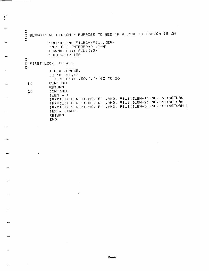
F
C
C SUBROUTINE FILECH - F'URF'OSE TO SEE IF A ,.SDF EXTENSION IS ONC
SUBROUTINE FILECH(FILI_ IER[MF'LICIT INTEGER*2 I-N)CHARACTER*I FILl 1"'
I..OGICAL*'2 IER
C
C FIRST LOOK FOR A
C
IER = .FALSE.
DO i(').I=l,l "_
IF (FILl(1) .EQ. GO TO 2(')
CONT INUE
RETURN
CONTINUE
ILEN = I
IF(FILl (ILEN+I).NE. 'S' .AND. FILl (ILEN+I).NE. 's')RETURN
IF(FIL!(ILEN+2).NE. "D' .AND. FILI(ILEN ).NE. 'd')RETURN
IF(FILl (ILEN+3).NE. 'F' .AND. FILl (ILEN+3).NE. '_')RETURN ,
IER -- .TRUE.
RETURN
END
B-46

CC SI]BROUTINEFILEM - TO CONSTRUCTA FILENAMEC
SUBROUTINEFILEM(F!LI,FIL2,FX,INUM,ILEN)IMPLICIT INTEGER*2 (I-N)CHARACTER*I FILl(12) ,FIL2(12) ,FX(3)CHARACTER*2ANUM
CC WRITE OUT I NUMTO ANUMC
WRITE(ANUM,900)900 FORMAT(12)
C
INUM
C CALL FILCHG TO GET FILENAMEC
CALL FILMAF'(FILI,FIL2,FX,ANUM,ILEN)RETURNEND
¢
+
B-47
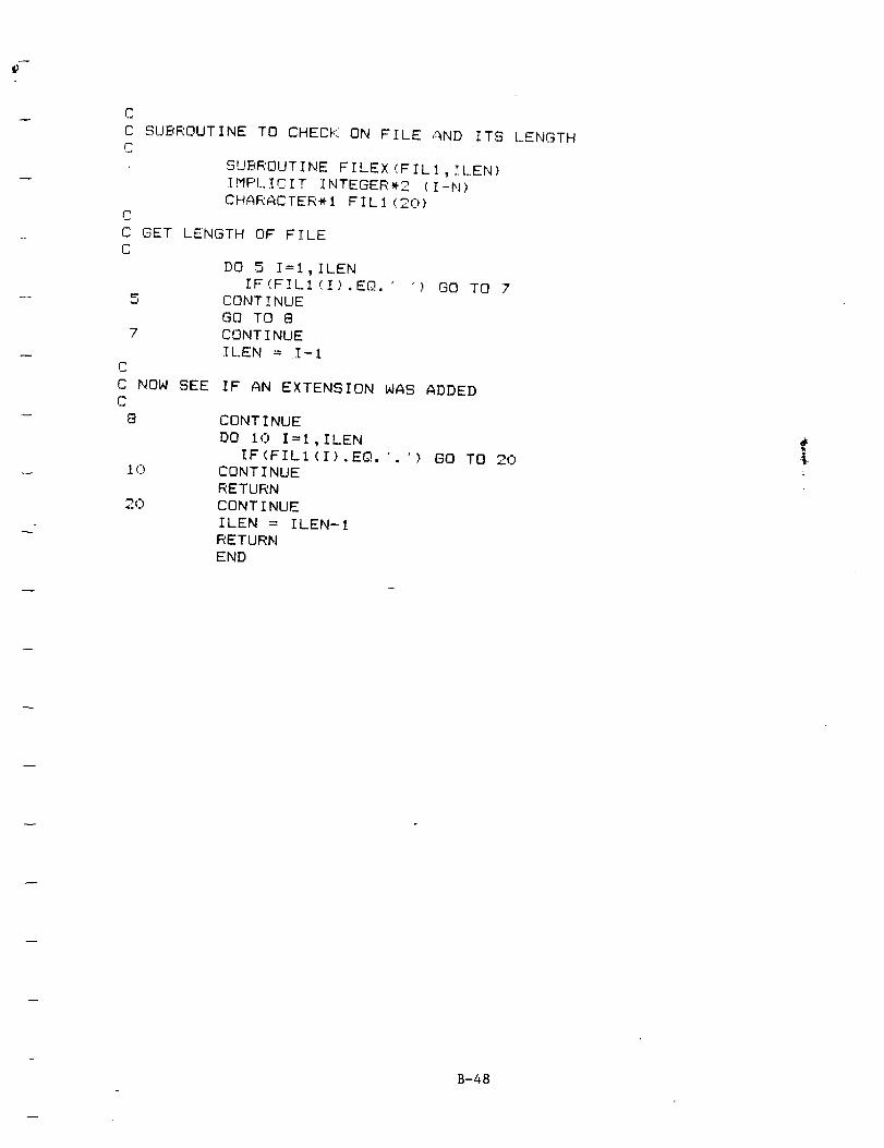
CC SUBROUTINETO CHECKON FILE AND ITS LENGTHC
SUBROUTINEFILEX(FIL1, !LEN)IMF'LICIT INTEGER*2 (I-N)CHARACTER*I FILl (20)
CC GET LENGTHOF FILEC
DO 5 I=l, ILENIF (FILl (I) .EQ. " ") GO TO 7
5 CONTINUEGO TO 8
7 CONTINUEILEN = I- 1
CC NOWSEE IF AN EXTENSIONWASADDEDC
8 CONTINUEDO I0 I=I,ILEN
IF(FILl (I).EQ. '. ') GO TO 201o CONTI NUE
RETURN20 CONTI NUE
ILEN = ILEN-IRETURNEND
B-48

C
C SUBROUTINE FILMAP - TO CONSTRUCT A FILENAME
C
C
C
C
C
10
15
CALLED FORM FILEM
SUBROUTINE FILMAP(F!LI,FIL2,FX,ANUM,ILEN)
!MF'L.ICIT INTEGER*2 (I-N)
CHARACTER*I ANUM(2),FX(3>,F!LI(12),FIL2
2(])
C
C CHANGE BLANKS TO ZEROES
C
NLEN = ILEN + 6
DO 30 I=I,NLEN
IF(FIL2(1).EQ. '
30 CONTINUE
RETURN
END
DO 10 I=I,ILEN
FIL2(I) = FILl(I)
CONTINUE
DO 15 I=1,2
FIL2(ILEN+I) = ANUM(I)
CONTINUE
FIL2(ILEN+3) =
DO 2(i) I=1,3
FIL2(ILEN+3+I) = FX(I)
CONTINUE
'> FIL2(I> = "0'
12)
B-49
OF POOR QUp, L_,?/

|w
C
C SUBROUTINE MACDAM - MACRAN FFT CARD
C
SUBROUTINE MACDAM(TITLE)
_MF'LICIT INTEGER*2 (:[-N)
INTEGER*2 ICHNI<IO),ICHNO(14)CHARACTER*f2 FILIN(1)
CHARACTER*30 TITLE
COMMON/NASADT/ICHNI,ICHNO,NINPUT,NOUTPT,FILIN,NPNTS
60
100
C
C
C WRITE OUT STUFF
C
WRITE(10,8003) TITLE
I_003 FORMAT('JBHEAD ',A30,5X,
WRITE(10,8010) FILIN
8010 FORMAT('FILIN',2X,AI2)C
C HERE FOR INPUT CHANNELS TO BE FFT BY FOUR
C
IF(NINPUT.GT.3) GO TO 50
WRITE(10,9030) (ICHNI(IL) ,IL=I,NINPUT)
60 TO 100
50 CONTINUE
WRITE(10,9030) (ICHNI(IL),IL=I,3)NLINES = (NINPUT+I)/4
DO 60 IO=I,NLINES
IL = 4 + 4 * (IJ-l)
If( = IL + 3
IF(IK.GT.NINPUT) IK = NINPUT
, WRITE(10,9040) (ICHNI(IM),IM=IL,IK)
CONTINUE
CONTINUE
INPUT CHANNEL FOURIER TRANSFORMS')
C WRITE OUT FILOUT STUFF FOR MACRAN
C
WRITE (10,8020)
WRITE (10,8030)
WRITE (10,8040)
WRITE (I0,8050)
WRITE (10,8060)CC WRITE OUT MACRAN STUFF FOR OUTPUT CHANNEL FFT
C
WRITE(It;),8007) TITLE
8_;x;)7 FORMAT('JBHEAD ,A30,5X, "OUTPUT CHANNEL FOURIER TRANSFORMS'>
WRITE (1(),8010) FILINC
C HERE FOR OUT CHANNELS TO BE FFT BY FOUR
C
NOF'T = NOUTPT
IF(NOPT.GT. 127 NOPT = 12
IF(NOPT.GT.3) GO TO 150
WRITE(IO,9030) (ICHNO(IL) ,II_=I,NOPT)
GO TO 200
150 CONT INUE
WRITE(10,9030) (ICHNO(!L) ,IL=I,3)
B-50

F
! 6¢D2 0 0
C
C HERE
C
3 0 (')
NLINES = (NOPT+I)/4
DO 160 IJ=I,NLINES
IL = 4 + 4 * (IJ-1)
!K = IL + 3
IF (IK. GT. NOPT)
WRITE (io, 904A)
CONT INIJE
CONTINUE
WRITE (10,8070>
WRITE (10,8030)
WRITE (10,8080)
WRITE (10,8090)
WRITE (I0,8060)
IF,::= NOF'T
(!CHNO(IM> , !M=IL,IK)
IF MORE THAN 12 OUTPUT CHANNELS
IF(NOUTPT
WRITE <10
WRITE (I0
WRITE <10,
WRITE (10,
WRITE (I0
WRITE (10
WRITE (10
CONTINUE
WRITE (10,RETURN
C
C FORMAT SECT
C
9030
9(:)4(')
8020
8030
8040
8050
8060
8(370
8080
8090
7020
7040
7050
7070
.LE. 12) GO TO 300
8010) FILIN
9030) <ICHNO(IL) ,IL=I3,NOUTPT)7020 )
8030 )
7040 )
7050 )
8060 )
7cD70 )
ION
FORMAT('FILIN',IX,'CCHAN',I4X,• ' ' 12FORMAT('FILIN ,IX, CCHAN ,5X,4(9X, ,
FORMAT('FILOUT FORDI.SDF')
FORMAT('FOUR')
FORMAT('FILIN',2X,'FORDI.SDF')
FORMAT('FILOUT',IX,'FORDI.DAT')
FORMAT('CTAPE',52X,'-I.')
• .' 12I ,IX,3<9X, ,
.'))
FORMAT('FILOUT FORDOI.SDF
FORMAT('FILIN FORDO1.SDF
FORMAT_'FILOUT FORDOI.DAT. -
FORMAT_'FILOUT FORDO2.SDF
FORMAT('FILIN FORDO2.SDF
FORMAT('FILOUT FORD02.DAT
FORMAT('END')
RETURN
END
"))
Ji
?
B-51

d$i
S
C SUBPOUTINE MACCRDI -- F'UF;F'OSE TO WRITE OUT FIRST MACRAN CARD
SUBROUTINE MACRDI (FILIN,NINF'UT, ICF-INI, iCHNO,T!TLE,NF'NTS>
I_,F'LIC!-[ INTEGER*2 (I-N)DIMENSION ICHNI (i__>
CHARACTER* 12 FILIN
CHARACTER*30 TITLE
C
C WRITE OUT FIRST COUPLE OF COMMENT CARDS
C
!4RITE (10,9010) TITLE
q010 FORMAT( 'JBHEAD ',A30,5X, 'TRANSFER FUNCTIONS')
WRITE (10,9020> FILIN
9020 FORMAT('FILIN' ,2X,AI2)
C
C NOW WRITE OUT CHANNEL NUMBERS
C
IF(NINF'UT.GT.2> GO TO 5¢:)
WRITE(10,9030) ICHNO, (ICHNI (IL> ,IL=I,NINPUT>
GO TO 1O0
50 CONT INUE
WRITE(10,9030) ICHNO, <ICHNI(IL) ,IL=I,2)NL!NES = (NINF'UT+I)/4
DO 60 IJ=I,NLINESIL = 3 + 4 * (IJ-l)
IF:.'.= IL + 3
IF(IF=:].GT.NINPUT) IF-':'.= NINPUT
WRITE<I0,9040) (ICHNI(IM) ,IM=II_,IK)CONTINUE
FORMAT('FILIN',IX, 'CCHAN', 14X, "I. ', IX,3(9X,I2, ". "> >
FORMAT('FII_IN',IX,'CCHAN',5X,4(9X,12, . '>>
6(:)
903(:)
9040
C
C HERE FOR REST OF DATA
C
100 CONTINUE
WRITE(10,9050) NPNTS
9050 FORMAT(
! "FILOUT MATRXD2.SDF'
2/'PSD TRANS',IIX,14,3/'PSD TOUTMTFC'
4/'PSD RETAIN'
5/'END'
6/>
RETURN
END
,19X, '6. ,
B-52

CC SUBROUTINEMACCRD2- F'URPOSETO WRITE OUT 2ND MACRANCARDC
SUBROUTINEMACRD2IMPLICIT INTEGER*2 (I-N)
CC WRITE OUT STUFFC
WRITE<I.o, 90 i0)9010 FORMAT('FILIN MATRXD2,SDF'
1 /'FILOUT TRNSMD2.SDF'
._ ,/'TRANS TAPE "
3 / 'END'
4 /)
RETURN
END
B-53

CC SUBROUTINEMACCRD3- PURPOSETO NRITE _]UT 3RD MACRANCARDC
_UBROUTTNEMACFD3IMPLICIT INTEGER*2 (I-N>NRITE( !0 _9010>
9010 FORMAT(_FILIN TRNSMD2.SDF'
! / _FILOUT HD2.DAT•
2 /'CTAPE',52×, '-i "3 / "END'
4 /)
RETURN
END
B-54

CC FROGRAMNASA - PURPOSE: TO CREATEA BATCHP'ILE
WHICHWILl_ EXECU_EMACRANSEVERALTIMESCC
CC
IMPLICIT INTEGER*2 <I-N)DIMENSION ICHNI <i0) ,ICHNO(14)CHARACTER*80KEYCHARACTER*30TITLECHARACTER*I2 MFILI!,MFILIO,MFIL21,MFIL20CHARACTER*f2 MFII_31,MFIL30,MFIL41,MFII_40CHARACTER*I2 FILIN,FILOTI,FILOT2CHARACTER*6MFILI _MFIL2,MFII..3,MFII_4,FILOTCHARACTER*3FXI,FX2,FX3,FX4,AYNCHARACTER*I ATYPE,FILET(12)LOGICAL*2 EXISTS, IERCOMMON/NASADT/ICHNI, ICHNO,NINPUT, NOUTPT,FILIN, NPNTSEQUIVALENCE(FILOT2,FILET(1))
CALL VCLEARCALL VCURXY(0,0)
CC DISPLAY PROGRAMNAMETO USERC
KEY = 'PROGRAMNASA - TO GENERATEA MACRANBATCH FILES"CALL PRMPT(KEY,I. 10)
CC BEGNIN HERECCC OPENUP FILE CONTAINING NPTSC
OFEN(31 ,FILE= ' INTRFS. DAT' )READ(31,8831) NPTS
8931 FORMAT(I4)NPNTS = (NPTS+3)/4IR = 7
1__ CONTINUEKEY = 'ENTER INPUT MACRANFILENAME (INCLUDING .SDF) : $"CALL KEYBD(KEY,R,I,FILIN,3, (12) ,O,IR)
CC SEE IF FILE EXISTSC
INQUIRE(FILE=F I LIN, EXIST=EXISTS)IF (EXISTS) GO TO 15IR = IR + 1CALL VCURXY(O,IR)WRITE(*, 901r))
9r)10 FORMAT(IX,_FILE DOES NOT EXISTS - PROGRAMABORT!!_)STOP
CC MAKESURE IT HAS A .SDF EXTENSIONC
15 CONTINUEIR = IR + 1CALL VCURXY(O,IR) B-55

WRITE(*,8543) NPTS,NPNTS8543 FORMAT(IX, 'NUMBEROF F'OINTS : , I4,
1 /IX, 'NUMBER OF F'O!NTS/SEGMENT ; _I4X)
CALL VCURXY(O, !R)
C.AL.L F!L.ECH(F!LIN,IER?!F(!ER) GO TO 20
IR = IR + 2
CALL VCURXY(O,IR)
WRITE (* ,9002)
9002 FORMAT(IX, "NO .SDF EXTENSION -- PROGRAM ABORT!!')
STOP
C
C HERE IF OK
C
20 CONT INUE
!R = IR + 2
KEY = 'ENTER OUTPUT FILENAME - NO FILE EXTENSIONS F'LEASE :$"
CALL KEYBD(KEY,R,I,FILOT,3, (6) ,O,IR)
C VERIFY NO EXTENSION AND GET CURRENT LENGTHC
IFLEN = 6
CALL FILEX(FILOT,IFLEN)
NFLEN = IFLEN + 6
C
C NOW GET INPUT/OUTPUT CHANNELS
903c)
40
9031
C
30
45
C
C NOW GET OUTPUT CHANNELS
C
48 CONTINUE
CALL VCLEAR
IR = 2
CONTINUE
IR = IR + 2
CALL VCURXY(O,IR)KEY = 'ENTER THE NUMBER OF INPUT CHANNELS (<= 10 ) :$'
CALL KEYBD(KEY,R,NINPUT,A,2, (2),O,IR>
IF(NINPUT.LE.10) GO TO 40
IR = IR + 1
CALL VCURXY(O,IR>
WRITE(*,903c))
FORMAT(IX,'TO0 MANY INPUT CHANNELS SPECIFIED'\)
GO TO 30
CONTINUE
IR = IR + 2
CALL VCURXY(O,IR)
WRITE(*,9031)
FORMAT(1X,'SPECIFY MACRAN CHANNEL TO USE FOR EACH INPUT'\)IR = IR + 1
CALL VCURXY<O,IR>
KEY = '--> $'
DO 45 IC=I,NINPUTIR = IR + 1
(2) 0 IR)CALL KEYBD(KEY,R,ICHNI(IC),A,_, , ,
CONTINUE
B-56

CALL VCURXY(O,IR)KEY = 'ENTER THE NUMBER OF OUTF'UT CHANNELS ( <= 14 ) :_'
CALL KEYBD(KEY,R,NOUTPS,A,2. , (_)_.,0, IR)IF(NOUTF'T.LE. 14) GO TO 50
IR = IR * I
CALL VCURXY(O, IR)
WRITE (*,9040)
9040 FORMAT(IX, 'TO0 MANY OUTPUT CHANNELS SPECIFIED'\.)
GO TO 48
(]
C NOW GET OUTPUT CHANNELS
C
5c') CONTINUE
IR = IR + _o
CALL VCURXY(O,IR)
WRITE (*,9()41)
9041 FORMAT(IX, "SPECIFY MACRAN CHANNEL FOR EACH OUTPUT'\)
IR = IR + I
CALL VCURXY(O,IR)KEY = '--> _.'
DO 55 IC = I,NOUTPT
IR = IR + 1
CALL KEYBD(KEY,R, ICHNO(IC) ,A,2, (2) ,O,IR)
55 CONT INUE
C
C SEE IF A DAMAGED OR UNDAMAGED CASE
C
IR = IR + _.o
CALl_ VCURXY(O,IR)54 CONTINUE
KEY = 'IS THIS A (D)AMAGED OR (U)NDAMAGED RUN? :$'
CALL KEYBD(KEY,R,I,ATYPE,3, (i) ,c]),IR)IF(ATYPE.EQ. 'D" .OR. ATYPE.EQ. "d') GO TO 56
IF(ATYPE.EQ. "U' .OR. ATYPE.EQ. _u') GO TO 56
GO TO 54
56 CONTINUE
C
C GET TITLE FOR THIS RUN
C
KEY = "ENTER A DESCRIF'TIVE TITLE FOR THIS RUN : $'
IR = IR + 2
CALL KEYBD(KEY,R,I,TITLE,3, (30) ,O,IR)
C
C
C
NOW START CREATING THE BATCH FILE
OPEN(6,FILE='NASAD.BAT',STATUS='NEW')
OPEN(7,FILE=_NASAREN.BAT',STATUS='NEW ")
OPEN(8,FILE=_MATRX.DAT',STATUS='NEW ' )
WRITE(8,4010) NINPUT,NOUTPT,ATYPE,TITLE
4010 FORMAT(15,2X,IS,2X,AI/A30)
C
C ASSIGN GENERIC FILENAMES TO MACRAN FILES
C
MFILI = 'TRNSDI"
MFIL2 = 'TRNSD2"
MFIL3 = 'TRNSD3' B-57
MFIL4 = 'TRNSD4'
FXI = 'INP"
F×2 = 'OUT"
FX3 = "SDF'
FX4 = "DAT"
IL = 6
C
C NOW LOOP OVER "FHE NUMBER OF OUTPUT CHJANNELS TO PROCESS
C
DO i00 ICHN=I,NOUTF'T
C
C GET FIRST MACRAN FILENAME
C
CALL FILEM(MFILI,MFILII,FXI,ICHN,IL>
OF'EN(10,F!LE=MFILII,STATUS='NEW')C
C NOW WRITE OUT FIRST MACRAN CARD
C
CALL MACRDI(FILIN,NINF'UT,ICHNI,ICHNO(ICHN),TITLE,NPNTS_
CI_OSE(10,STATUS='KEEF")
CALL FILEM(MFILI,MFILIO,FX2,ICHN,IL)
C
C GET SECOND MACRAN FILENAME
C
CALL FILEM(MFIL2,MFIL2I,FXI,ICHN,IL)
OPEN(10,FII_E=MFIL21,STATUS='NEW')C
C WRITE OUT SECOND CARD
C
CALL MACRD2
CLOSE(10,STATUS='KEEP')
CALL FILEM(MFIL2,MFIL20,FX2,ICHN,IL)
C
C GET THIRD MACRAN FILENAME
C
CALL FILEM(MFIL3,MFIL3I,FXI,ICHN,IL)
OF'EN(10,FILE=MFII_3I,STATUS='NEW')
C
C WRITE OUT THIRD MACRAN CARD
C
CALL MACRD3
CLOSE(IO,STATUS='KEEP')
CALL FILEM(MFIL3,MFIL30,FX2,ICHN,IL)C
C NOW ADD TO THE NASAD.BAT FILE
C
WRITE(6,6010> MFILII,MFILIO
WRITE(6,6060) MFIL2!,MFIL20
WRITE<b,6010) MFIL31,MFIL30
C
C GET OUTPUT FILENAME
C
CALL FILEM(FILOT,FILOTI,FX3,1CHN,IFLEN)
CALL FILEM(FILOT,FILOT2,FX4,1CHN,IFLEN)C
C WRITE OUT BATCH COMMANDS B-58

4020C
150C
WRITE(6,6020) FILOTI,F LOTIWRITE(6,6030) FIL.OT2,F I..OT2
WRITE(8,4020) (FILET(IFM , IFM=t,NFLEN)CONTI NUE
FORMAT (12AI )
IF(IFLEN.EQ.6) GO TO 150
CALL FILAD(FIL.OT,IFLEN)
CONT INUE
C FINISH OFF BATCH COMMANDS FOR NASA.BAT
C
WR ITE (6,6¢')7(::)
C
CLOSE (6, STATUS= 'KEEP ')
C
C NOW ADD TO NASAREN. BAT
C
WRITE (7,6050) FILOT,FILOT
CLOSE (7, STATUS= 'KEEP' )C
C END IT ALL
C
CLOSE (7, STATUS='KEEF'" )
CALL VCURXY(0,23)
STOP
C
C FORMAT SECTION
C
6010
6020
6030
6040
6045
6046
605(]
6060
6 07 0
FORMAT('MAC423 !R 1(:)000 :'',AI2, ' :::',AI2)
FORMAT('DEI_' _IX,AI2/'REN TRNSMD2.SDF',IX,AI2)
FORMAT('DEL' ,IX,AI2/'REN HD2.DAT' ,IX,A12)
FORMAT('DEL',IX,A6, 'OI.BFT'
/'REN FORDI.DAT', IX,A6, 'OI.BFT')
FORMAT('DEL',IX,A6, 'OI.DFT'
/ REN FORD(:)I.DAT' _IX_A6, 'OI.DFT')
FORMAT('DEL' wlX_A6, '(:)2.DFT'
/'REN FORD02. DAT',IX,A6, '02.DFT')
FORMAT('DEL' ,IX_A6, '.BAT"
/'REN NASAD.BAT', IX,A6_ .BAT')
FORMAT('MACTRN /R 100()0 <',AI2_ " >' ,AI2)FORMAT ( 'TESTRD. EXE "/ "NASAREN. BAT ')
END
B-59

_NOFLOATCALLS
IMPLICIT INTEGER*2 (I-N)
COMPLEX*8 TFU(I-_,10) ,TFD(I-/_. I0)
COMPLEX*8 DAM (7,2500)
OIMENSION ILMI (14) _ILMO(14)CHARACTER*80 KEY
CHARACTER*30 TITLE
CHARACTER*20 TFUF_TFDF
CHARACTER*I ATYPE
COMMON/DAMC/TFU, TFD ,DAM, ILMI , ILMO,NINF'UT, NOUTPT
C
C
C
CALL VCLEAR
CALL VCURXY(0,0)IR = 0
C
C GET EACH FILENAME,OPEN IT UP AND READ HEADER INFO
C
TFUF = 'HWUMAT. DAT'
OPEN(6,FILE=TFUF,FORM='UNFORMATTED'>
READ(6> TITLE,NFREQ,NINPUT,NOUTPT,ATYPE,DELF
WRITE(*,9000) TITLE,NINPUT,NOUTPT,NFREQ,DELF
9000 FORMAT(IX,A30
1 /IX,'NUMBER OF INPUT CHANNELS
IIX, 'NUMBER OF OUTPUT CHANNELS • '
3 /IX,'NUMBER OF FREQUENCY POINTS
q /IX,'FREQUENCY STEP SIZEIR = IR + 6
CALL VCURXY(O,IR)
IF(ATYPE.EQ.'U" .OR. ATYPE.EQ. 'u')
,14
,14
,14
,IPEIO.3,' HZ'\)
WRITE (*,9010)
IF(ATYPE.EQ. 'D' .OR. ATYPE.EQ. 'd•) WRITE(*,9015)
9010 FORMAT (IX, 'UNDAMAGED •\)
9(])15 FORMAT(IX,'DAMAGED'\)
IR = IR + 2
CALL VCURXY(O,IR)
C
C GET DAMAGED TF FILENAME
C
TFDF = "HWDMAT.DAT'
OPEN(7,FILE=TFDF,FORM='UNFORMATTED')
READ(7) TITLE,NFREQ,NINPUT,NOUTPT,ATYPE,DELF
WRITE(*,9000) TITLE,NINPUT_NOUTPT,NFREQ,DELF
IR = IR + 6
CALL VCURXY(O,IR)
IF(ATYPE. EQ. 'U • .OR. ATYPE.EQ. 'u') WRITE(*,9010)
IF(ATYPE.EQ.'D" .OR. ATYPE.EQ.'d') WRITE(*,9015)IR = IR + _
C
C SEE ABOUT ROW/COLUMN ELIMINATION
C
PAUSE
CALL VCLEAR
IR = 0
CALL VCURXY(O,IR)DO 40 I=I,14 B-60

4 0
9200
50
75
80100
C
ILMI (I ) = 0
ILMO(1) = (')
CONTINUE
KEY = HOW MANY INPUT CHANNELS DO YOU WANT TO ELIMINAT..=:
C{-_LL.KEYBD<KEY,R,IELMI,A,2, (o_._.,,(').,IF'.IR = IR + 1
IF(IELMI.EQ.O> GO TO 75
CALL VCURXY(O, IR)
WRITE (*, 9200)
FORMAT(IX, 'ENTER CHANNELS TO ELIMINATE \)IR = IR + 1
CALL VCURXY(O,IR>
DO 50 I=I,IELMI
KEY = '--> :_'
", r_ (') IR)CALL KEYBD(KEY,R,ILMI (I) ,A, , ,_-) , ,IR = IR + I
CONTINUE
CONTINUE
IR = IR + IKEY='HOW MANY OUTPUT CAHNNELS DO YOU WANT TO ELIMINATE? ! $"
(2) 0 IR)CALL KEYBD<KEY,R,IELMO,A, , , ,IF(IELMO.EQ.(')> GO TO 1(')()
IR = IR + i
CALL VCURXY(O,IR)
WRITE (*,92A0)IR = IR + 1
CALL VCURXY<O,IR)
DO 80 I=I,IELMO _I<EY = "--> $'
CALL KEYBD(KEY,R,ILMO(I> ,A,2, (2_,0,1R)
IR = IR + I
CONTINUE
CONTINUE
C NOW READ IN ALL THE DATA, ONE FREQ POINT AT A TIME AND COMPUTEC DAMAGE FOR THAT FREQ POINT
C
NTOT = NINPUT + NOUTPT
DO 150 IFQ=I,NFREQ
DO 110 IO=I,NOUTPT
READ(6> (TFU(IO,I),I=I,NINPUT)
READ(7) (TFD(IO,I),I=I,NINPUT)110 CONTINUE
CALL DAMCOM(IFQ)
150 CONTINUE
C
C CALL MACWRT TO WRITE OUT DATA
C
CALL MACWRT(DAM,NFREQ,DELF,TITLE)
C
C END IT ALL
C
CALL GCURXY(IC,IR)
IR = IR + i
CALL VCURXY(O,IR)
STOP B-61

I
END
P
I
B-62

-.k
!
SNOFIo.OATCALLS
SUBROUTINE DAMCOM(IFO)
IMPLICIT INTEGER,2 (I-N)
COMPLEX *8 TFU(14, i0) ,TFD(14, I0)
COMFL.EX*8 DAM (7,25r10) ,AUXI,AUX2,AUX3,AUX4,AUX5
DIMENSION ILMI (!4) , ILMO(14)
COMMON/DAMC/TFLJ,TFD,DAM,ILMI,ILMO,NINPUT,NOUTPTC
C ZERO OUT AUX
C
AUXI = (0. ,0.)
AUX2 = (C). ,0.)
AUX3 = (0. ,0.)
AUX4 = (0. ,0.)
AUX5 = (0. ,0.)C
C COMPUTE DAMAGE
C
DO 20 KK=I,NOUTF'T
DO 19 IK=I,NOUTPT
IF(KK.EQ. ILMO(IK) ) GO TO 20
19 CONTINUE
DO I0 JJ=I,NINPUT
DO ii IJ=I,NINPUT
IF(JJ.EQ. ILMI (IJ) > GO TO I0
CONTINUE
AUXI = AUXI + TFU(KK,JJ) * FTO(KK) * FTI(JJ)
AUX2 = AUX2 + TFD(KK,JJ) * FTO(KK) * FTI(J_)
AUX3 = AUX3 + TFU(KK,JJ) * TPU(KK,JJ)
' AUX4 = AUX4 + TFU(KK,JJ) * TFD(KK,JJ)
AUX5 = AUX5 + TFD(KK,JJ) * TFD(KK,JJ)10 CONT INUE
2(') CONT INUE
DAM(1,IFQ) = (AUX5 + AUX4) / (AUX4 + AUX3)
DAM(2,1FQ) = (AUX4 + AUX3) / (AUX5 + AUX4)
DAM(3,IFQ) = AUX3/AUX4
DAM(4,IFQ) = AUX4 / AUX3
DAM(5,IFQ) = AUX4 / AUX5
DAM(b,IFQ) = AUX5 / AUX4RETURN
END
II
C
C
PRECEL_i__G P,;_,3E ._-_,..,.'.:,-,,i'_;O_ F:!LMED
B-63
SNOFLOATCALLS
SUBROUTINE MACWRT(DAM,NFREQ,DELF,TITLE)
IMPLICIT INTEGER*2 (I-N)
COMPLEX DAM (7,2500> ,XDAM(7)REAL*4 RDAM(16)
CHARACTER*4 ADAM(7)
CHARACTER*30 TITLE
C
C SET UP CHARACTER STRINGS
C
ADAM(1) = "DAM1
ADAM(2) = 'DAM2
ADAM(3> = 'DAM3
ADAM(4) = 'DAM4
ADAM (5) = 'DAM5
ADAM(6) = 'DAM6
ADAM(7) = "DAM7
C
C OPEN UP OUTPUT DAMAGE.SCF FILE
C
OPEN (20, FILE= 'DAMAGE. SCF' ,STATUS= "NEW' )
C
C START WRITING OUT TO FILE
C
WRITE(20,9090) TITLE
9090 FORMAT('JBHEAD',IX, 'COMPUTED DAMAGE - ",A30)
WRITE (20,9050)
WRITE (20,9000)
WRITE (20,9010)
WR ITE (20,9020 )
DO 20 I=l ,6
DO I0 IW=I,2
WRITE(20,9030) ADAM(1)I0 CONT INUE
20 CONT INUE
DO 30 I=I,16RDAM(I) = 0.0
3(3 CONT INUE
CALL GCURXY<IC,IR)
IR = IR + I
CALL VCURXY(O,IR)
DO 100 IFQ=I,NFREQ
RDAM(1) = FLOAT(IFQ-1) * DELF
DO 40 I=l ,6
XDAM(I) = DAM(I,IFQ)RI = AIMAG(XDAM(1))
RR = REAL(XDAM(1))
RDAM(I*2) = RR
RDAM(I*2+I) = RI
40 CONT INUE
WRITE(20,9040) (RDAM(1) ,I=i,16)
100 CONT INUE
WRITE (20,9060)
CLOSE (20,STATUS= 'KEEP' )
9000 FORMAT('CTAPE',2X, "NASA 1311.05")
9010 FORMAT('CTAPE' ,2X, "DAMAGE ',16X, '13')
B-64

902090309040
123
90509060
FORMAT( 'CTAF'E " ,2X , "FREQUENCY "
FORMAT ( "CTAPE' ,2X ,A4)
FORMAT ( 'CTAPE' ,19X,4 (El i. 3,1X
/'CTAPE C' ,17X,4(EII.3,1X
/'CTAPE C' ,17X,4(EII.3,1X
/'CTAPE C' ,17X,4(EII.3,1X
FORMAT('FILOUT DAMAGE.SDF')
FORMAT ( 'END ')
RETURN
END
B-65

APPENDIX C
EXAMPLES OF MULTI-INPUT MULTI-OUTPUT MODULE
TRANSFER FUNCTION MATRIX FOR NUMERICAL
TWO BOUNDARY POINT PROBLEM

This appendix contains examples of multi-input multi-output (MIMO)
module transfer function matrix computations for the numerical two boundary
point problem. Three examplesare provided. They are listed as follows:
a comparison of MIMOmodule transfer function computation resultsfor absolute responses is made; undamaged state and two damage
leve)s are looked at_ the damage is outside the module; the
excitation of the global system is base motion;
2, a MIMO relative module transfer function matrix is presented for
the numerical example without damage; also, corresponding time
history gain [single-input single-output (SISC)) transfer function
modulus] and coherence (corresponding to the gain plots) plots are
presented; the excitation of the global system s base motion; and
3, a HIMO relative module transfer function matr x is presented for
the numerical example without damage; the excitation of the global
system consists of a single force applied to Node Point 5.
C-2

|
MIMO ABSOLUTE MODULE TRANSFER FUNCTION MATRIX
EXCITATION--BASE MOTION
C-3
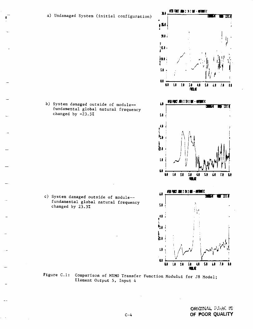
!a) Undamaged System (initial configuration)
i"!eo,oi
t
t
b,,°;|
to i
m FIIL'IillIIM)_III-_I¢
mm_x,W
i'
' I
7,r(
i
_- 4 ( +
/ ,,t '_i.
jtT, •i' i ' i
• i
l.o i,o _,o _o _o _,o i,o i,o_BE
b) System damaged outside of module--
fundamental global natural frequency
changed by -23.5%
ly Fill llll I lli l Ill • Illlll(.... i ira'mi,V
{4,t ;
h,o]
,l I
i
I,I! ,:,.,,/I
L! I .io _,o i.o
'\ L
l,@ U _l LO #.i L!lIB,i
c) System damaged outside of module--
fundamental global natural frequency
changed by 23.3%t#.
i
i
_,o,
I.I 4
M Ir(l(lillI INIi -lllllllC
.... _ imm'mx,d
'I ,_,
t/ttv'd
!ii
Li i • •lo i,o t,o i,o lo to i,o I.o lo
l|
Figure C.I: Comparison of MIMO Transfer Function Modului for J8 Model;
Element Output 5, Input 4
C-4 OF POOR QUALITY

p
a) Undamaged system (initial configuration) II,
lsot
l,I
! ;
:-4_i
-i_I
i
.... _ i mx,i
I
L
L
-Kl iII l.i i,t LI IO f,t i,O l,O lI
Illli
b) System damaged outside of module--
fundamental global natural frequency
changed by -23.5%
NIilIII-IIli°l .... _ i m_,i
I i
lLole l
,,
a
i I
I..i
lo f,o i,o i,o io i,o i,o ko loRaw
c) System damaged outside of module--
fundamental global natural frequency
changed by 23.3%
t
: /'--_, f ._,
t_'IU!, i ,, 4
I
._1
RIIIIIII-I
lo i,o i,o 3,o io i,o _,o i,o loItI
Figure C.2: Comparison of MIMO Transfer Function Phase for J8 Model;
Element Output 5, Input 4
C-5

a) Undamaged system (initial configuration) 10Lmwmlm2m mm_c
_'°_'°_! ' _uCm,,wi _,alI
_oi
_.!,
;I
s,oi, _ lj
i ,'% k
' T
o,o l Io,o s_oi,, _,o ,,,o i,o _,, 7,o I,o
FIn,E
b) System damaged outside of module--
fundamental global natural frequency
changed by -23.5%
RPrEI Nl INIlII-lllmlll(
]I,Ot .... l,nma_ m' mI,,I
m
let
ILl
¢Io,o Lo _o, _,o ,i,o_, i,o _,o m,o
FNI,ll
c) System damaged outside of module--
fundamental global natural frequency
changed by 23.3%
mlIIT m IINIgU -IlUll(
_,oI .... _ ram'_l,,_r
11'1!&
L,t I ) ,
u l
Figure C.3: Comparison of MIMO Transfer Function Modului for J8 Model;
Element Output 5, Input 7
C-6

a) Undamagedsystem (initial configuration) m_
L! ,
i-m!
-m(
-mqL!
III#I17m IIIIIII-illlllNl¢
]
J
i.o i.o _.o 4.o5.o _.o i.o totie
b) System damaged outside of module--
fundamental global natural frequency
changed by -23.5%
reel mlImIIN-IINI¢m.'; ' ' _ m m_,,
so,o!a
o.oi
1-4I
¢!
;I• II
(
i.o t*.o _o _.o s.oLo 1.o n.o
c) System damaged outside of module--
fundamental global natural frequency
changed by 23.3%
Figure C.4:
U
'_o,oi' t
"_.St
t
U
mfw ,i11tmIlml-Imll(
' ' ' ' _ mmt,_
_'N k
I6o t.o 3,o 4,o s,o Lo i.o n,o
fit,hi
Comparison of MIMO Transfer Function Phase For J8 Model;
Element Output 5, Input 7
_' C-7
OF POOR QUALITY

|a) Undamaged system (initial configuration) 6.1
q,tf\_,Oi
m RII_I.IIIIIIIi -lllllll(
!
ib
i
i
I.!
,,,i/0 1,0 Lt 3.! q.O 5,O 6.1
tll7,! L!
b) System damaged outside of module--
fundamental global natural frequency
changed by -23.5% o)q,!, !\
_,0
i.,
1,0
L0
m NlglIIIINIml-INlll(
.... _ m'm1,_
Li
o,o Lo to _.o i.o s.o_.o i.o toNm,!
c) System damaged outside of module--
fundamental global natural frequency
changed by 23.3%
Figure C.5:
6.1
U
4.0t
h,O
t.o
I,I
Lt
llg_Rl |ll'_(
.... _ m ran.tbq
r
LI i,l tl 3,t q,t _.l 6.1 7.0 8.o
Comparison of MIMO Transfer Function Modului for J8 Model;
Element Output 6, Input 4
C-8
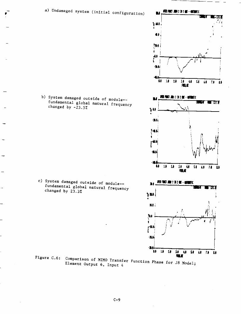
a) Undamaged system (initial configuration)
ql
40 iJ
+ !
,_oi r .L I /._ _
W
A
I
t
f',l' i
Vi,o 2.o i,o _o fo io 'i,o 'fi
b) System damaged outside of module--
fundamental global natural frequency
changed by -23.5%
L
c) System damaged outside of module--
fundamental global natural frequency
changed by 23,3%
Figure C.6:
-III • ,_0 t,0 t.0 i0 i,0 l0 +.0 i,0 fi
iim,nl
Comparison of M"IMO Transfer Function Phase for J8 Model+
Element Output 6, Tnput 4
C-9

+__
!+
a) Undamaged system (initial configuration)
b) System damaged outside of module--
fundamental global natural frequency
changed by -23.5%
R HII(I|L IIII| -dllml(
_O I .... _ i _|LW!
'!_,oJ
..o_ +'i,
+ ++,i.,\A
5,0 1
Jk! i , .
o+o_,ot,o _,o 4,o+,o_,o_,oLotlO
c) System damaged outside of module--
fundamental global natural frequency
changed by 23.3% W
_.0&
NIIulI Utl-lmmN
.... _ ram'ml._
i
q
i
!,
kO I.I I.I 3,I 4.I LI 6,1 P,O I,I:T ¸
Figure C.7: Comparison of MIMO Transfer Function Modului for J8 Model;
Element Output 6, Input 7
C-lO
• -.+._.,, +j",
OF POOfl _'; _t,,,._+,,,+,

d
a) Undamaged system (initial configuration)
-41
b) System damaged outside of module--
fundamental global natural frequency
changed by -23.5%
i
Loi
Itl llltl' ,1111In2lUll- gwI¢m mn.,I
A
-SI,I
-mlo,oi,o t,o _,o,.o s,o_.o i,o n,oFill
c) System damaged outside of module--
fundamental global natural frequency
changed by 23.3%
ID I_EI it l II t HI - fllal¢
lto, oa I
ItOt _, tJ i
u i,o i,o _.o _o to i.o _,o toFit
Figure C.8: Comparison of MIMO Transfer Function Phase for J8 Model;
Element Output 6, Input 7
C-It

MIMO RELATIVE MODULE TRANSFER FUNCTION MATRIX
EXCITATION--BASE MOTION
C-12

I
!
<==V
-=,,-
!
r,.,>------
I
s.
i
.... _____=.
i
Mr
J
_m
m
r
O-_--rd
i
I I
| !
m
m
m
!
X
- K----,Cr,
n
m
C-13

!
V
=n-
I
Z
0
r
4
r_
r ,,
r..._
r
--__2
:m
m --
" ...____._
w_I
|
"-""4
ll_In TT--
m
!
!
!
Fw_
n
m
n
m
i
!
C-14
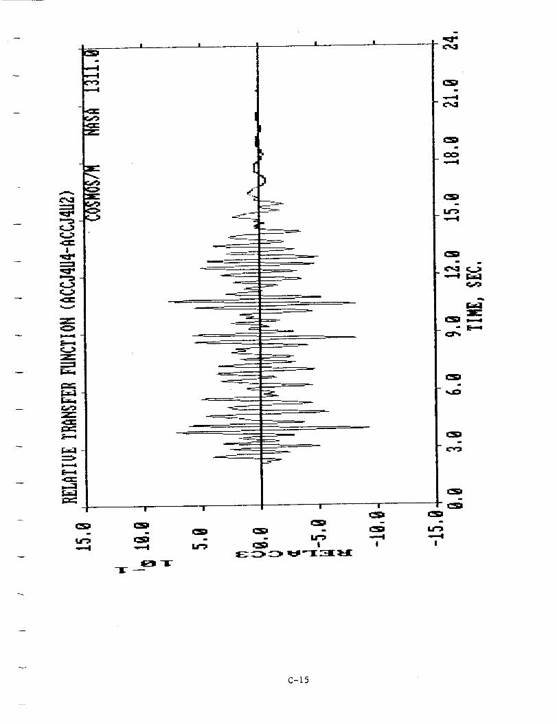
!
V
==;
_!
E
=i
o-r
B
r
!
m
m
i
E
m
m
n
!
C-15
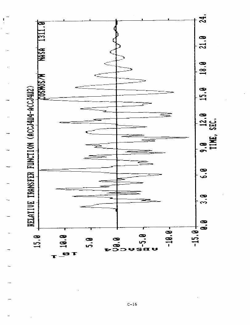
!
:I
,,,,-_
!
,_=_.
V
,:==,
..=,,.-
! !
n
_J
---=:_
w
|
T--
q
! !
r _
_.-.-.___...._.
| II
- _ "-'-4! !
-,..-4
I
-,--I
m
,m
-cr-_
m
I
m
!
C-16
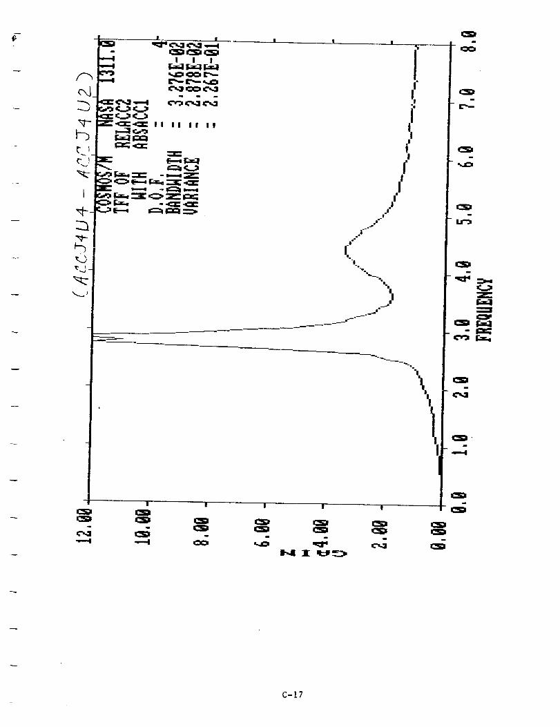
! I I q
! I !
II II II
I I I I
1--4 I ,_1'_
C-17
m
m
m
w
==1
- I_
m
°
m
-,--,d

I
:Ira
i
.=--I
,.-==I....-I
,.--.4
4:E ,:.._ <...:,
r.._..1i:X:_l
,c_ ._. [==-., I_E ,--.,
<...:, <..:,
l
I I Ir.._..I IF..T-1[.._..1
_=.-=.C--=.. ,..i_,
I II Ill !I
. ,..=..., -_a,-
- _ i-=-.a
I IL !
il°
,[_=.-
i II II l l
T __
.i-=I
O-I£-
I
m
m
m
ZC.T..1"=--I
_ [.._.I--
_,"_ _
m
m
C-18
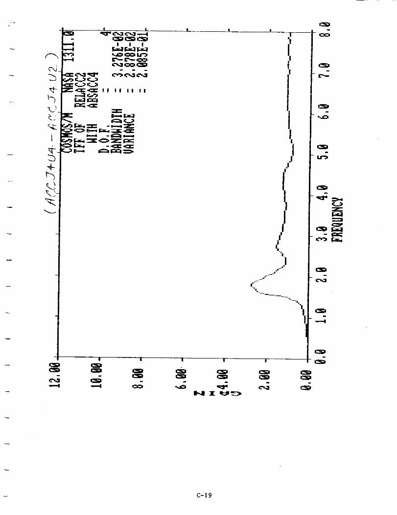
(''x
_-.)
_J
t
+%
i_Sll ' '
_-I ! ! !
__ I I I I I I I I
r-,,T-,lI=i::li==_;,,tU=
II II
!
I
!!
I¢1j
!
7Hi.
"i_
._...J_ll
|= •
"l
| I I
i
m
i
C-19

r ..L
m
! ! ! !
! ! I
I I! II II
I ! l I I
IE) TT--
m i m m
m
m
m
Z
- I_z:;
!
i
",--,4
C-20

.i-
H
i
-..-.l
,,-.4=-ll
1 1 q I I
I I I[.1111[.1Tlll[.ltl.1".._I "..l_l C''l"
II II _.I
'--r.-
_ _ _.-,_=T..,"l'ar.,_=,.i., ._ ,....,
e..,,__i.,"l'r0 _ _=m::OF.w-, --,_= .,==
,II
,f
iiI/I!
z
mI
!
I,i'}a|
N.__.--==
I
¢-
i i I
i..
o
li.
"=="4m m
n.-.1 I
|
m
I I
I
C-21
m
w
m
-I_
i
..i.=I

,:q
,..--4.---=4
¢.._i ¢_:, ¢,.:I
r..,T..]l:Z:li==:; ..,_
E
.=_=,¢;=. i_,-iiE ,,-,-,
,=_=.,=_=,c.,_ ¢_.i
:l" ,-:'_3,C'_3.=-==I
I I Ir,.,1r-] IF.,Ir,._IF.,,1r,_
¢"...1¢'...1¢'...1
¢','_I ¢'Y'_¢',,..1
'I II II II
....i-,I[--, ¢.lr..ll=Z=l It.__:'
- I=_I e,,,--e_, "_I.'- I_=:;
lb.-
|II
ll-
i
,:'...1..-=4
..
I
m
lll_
".='--4
alE_TT--
, i'- , ,
a _ m_ _ .:"-3
3 :::) N 3:1_1[ 3 H 0 ::)'
m
m
m
I
_ r-lr..1
I
,,,--I
-- C-22

_L
"m-
.,--4
.,.-4
.,---I
_IF''CII_'I_I_I I
r.a_la=l
I I I I,,_I14_-,_iIT,._.,--.i
I I Ir.-T-1_I.1 r,1.1t..1_ "..1_ 1.1"_
II II II
F.,__ "_-- - ,--.,-_-
_-- ,.__, . _,.-,
_, _.._.., -__._ E----, I:_11_Q _,.
|
•,---4 -,--4i
1",41 I
!
ii
! I
I'
./[
q
.°__q
(-
"|q
I
m
n
m
m
m
Z
m
-,--I
-- C-23
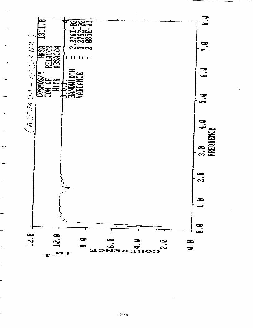
.---4
! ! !
I
! !! II I!
al_ -&--T--
i
i
I i I !
m
-'-"T _ H :3[ _d[ --'-::! H ,CI, ::3,
C-24

I
riR_*w
m
",""4
I ! l I |
m_-I
1-
--_=_
m ___ L-
"1
|
!.J"
-%
"l.ii
_--
I
r _
,-,,-!
I I I I
T II_ ::1:::i[..]L -,-I"--,C_,(_,I,,,il
i
m
IL"--
m
m
- r..T...
m
i
'--'.4
u
C-25

p
I ,....4I
C-26
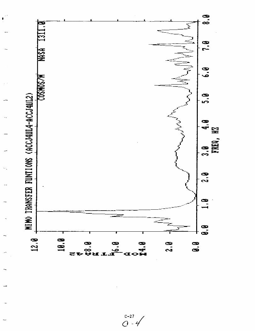
---m
r._.:mr.._:l
I
...-j
V
O
Z--,i-
..-,-4
m
,.--,4.pC
E"-..._
E
---j
--t--_-i
I
_m
-!-|
|.--
..I!
..m
.J
I|
-=- .
,/
,!
I%
)'L
I | | I m
l_m
J
n
m_m_m
i
D
i
l_m
X
mC_m
m
m_mi
m
-.--.,l

I
,-..1
I
I:_:I
Z....-..i
E
E
m
! W ! _--
E
I ! !
h-
-IKI_T
f'
|n m
_..
:;_II_"II=PI_I[_T__.T--Z Hcl[
m
I
C-28

I
!
V
Z
Z
-,w-IP,---[
.,Jr-
_D
.,--4,--.4
E
E
! ! ! I !
| i !
T nl_ ::l::J[ ..1[._,-T---<1_ 4_, II,,,B
C-29

!
I
V
Z
Z
0
m
ira.
| |
L •
,-._
.-=--.q
I
|
ram.
ill;"
I"
°
|'i
t.I
t
i
| |
I
|
I I
I
I
i
i
N
i
C-30

!
v
L
E.-.....
,0
i
e_
C-31

I
-cEI
V
Z
E
|
m
ai_
Iml:l
,,.--iii
l,X-:l..--.,.i
i
C-32

MIMORELATIVEMODULETRANSFERFUNCTIONMATRIXEXCITATION--FORCEAT NODEPOINT5
C-33

I
_- _ "1__
d J
q
----. !
I
=,--.4
._!
%
j1i
L..--
,, ia
!
_m
b --n_ _ _ --_|
-u
.... -"L
r
"f.
r
. .--
n-----_
! f -d F
!
f,.._!
!m
.%
- r..T.,
.,--I
C-34
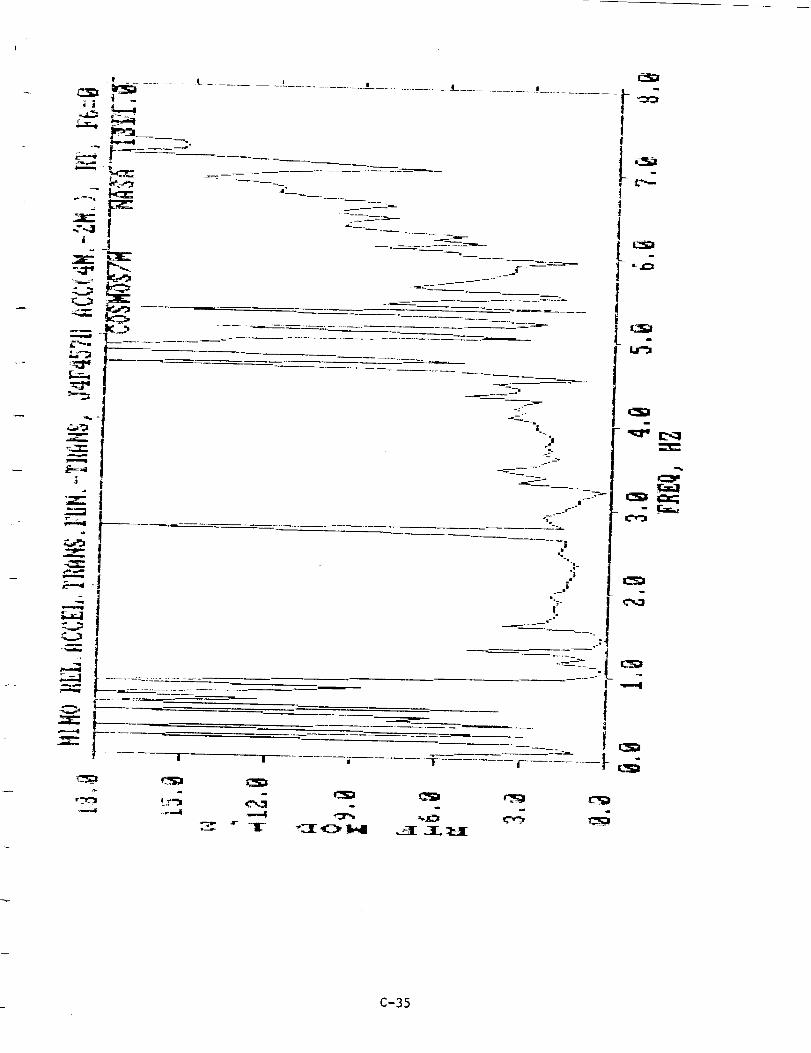
I
|
_,,,..,1i
m :I |................................. L ....
q."_--" -
l!!
i
_.-.,..
_,_,_,_,_,_,_,_,_,___
="IP"
_q
Z
o|
-__--_-:
°|
.=_
et
t
"2-;"
1
--4
!
I||
__--'t'2_
w
C-35
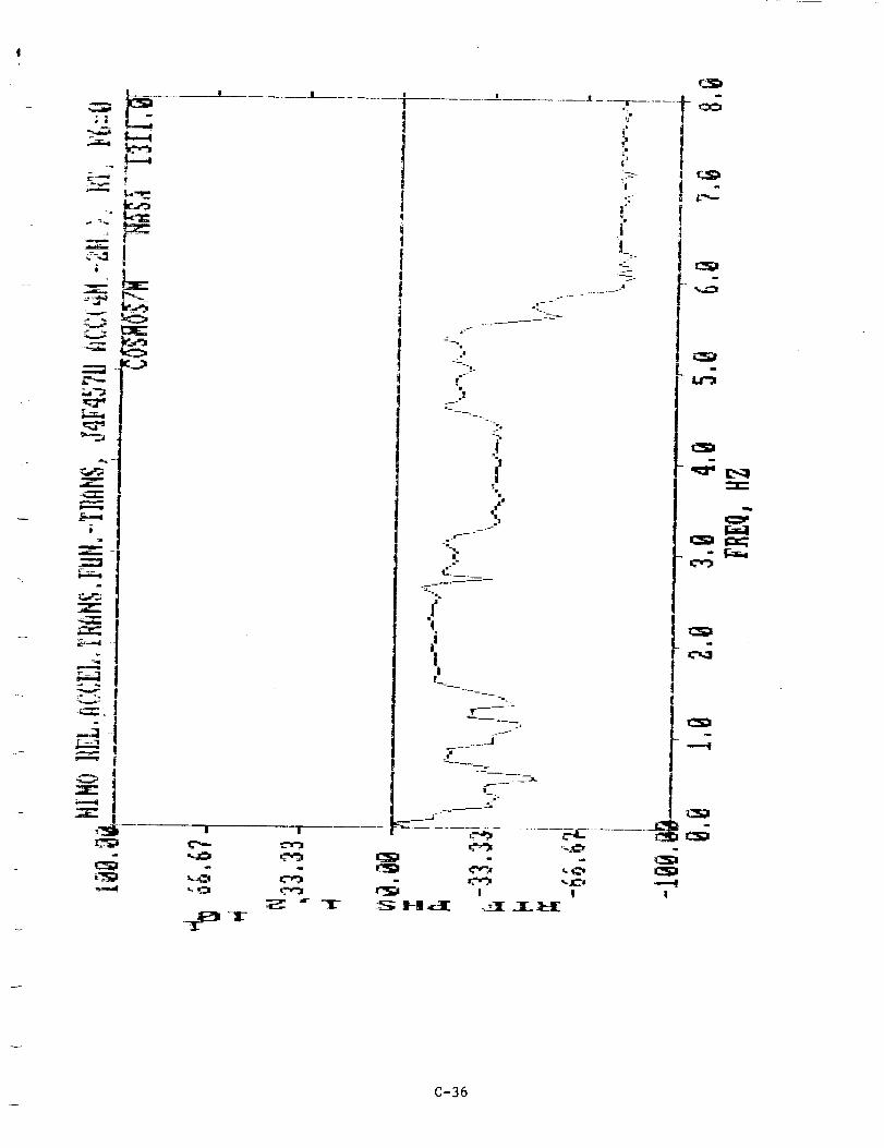
_--.j
!
•--.-, |
II
._1_ -1L-
I
u
:;E_ " -'JL-
1
IJ
If1
I
!.i
.--
--_--
---i t
.!
i"
_wg
%|i"C.
"T
--a
j."!
i
i--q
I m
"-'7_--.----'.-C
! !
m
.----,4!
C-36

i
_III "I"
_--3!
|
i
O"I--
J- ............... I
|_ -
I!iI
i
i
Ii.
itl
L I---" I_
'!_._,
_e-.1
2-
|
------m .°||
,=2
|1 m
!
.-"Y_7.
m_
m
"*,,.-4
I
-_ZEO I_4
C-37
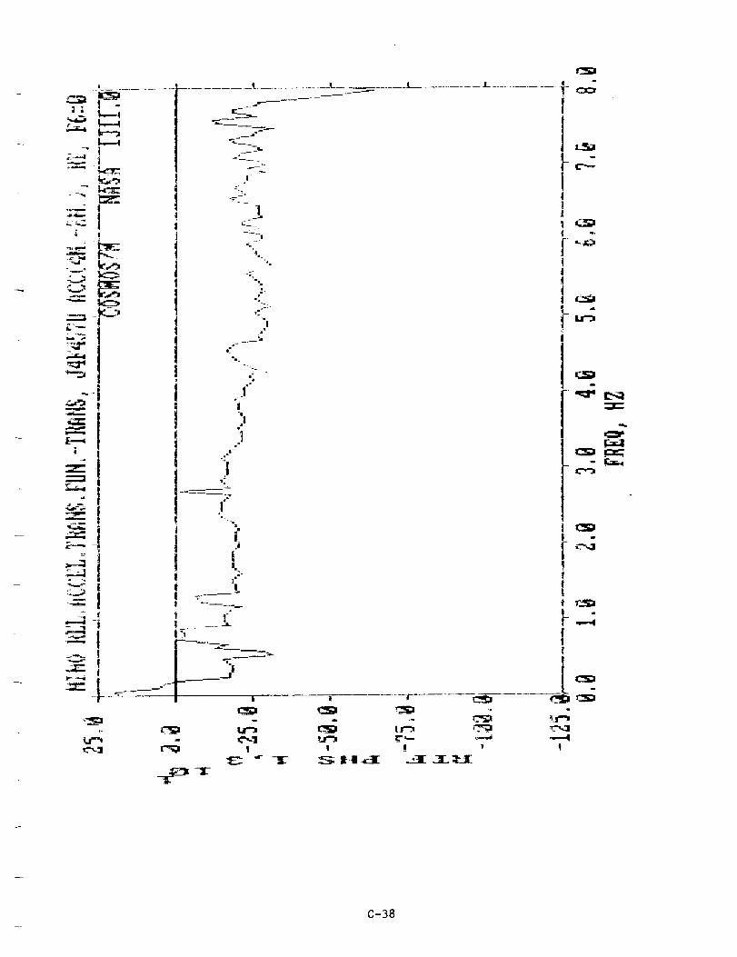
-I
C-38
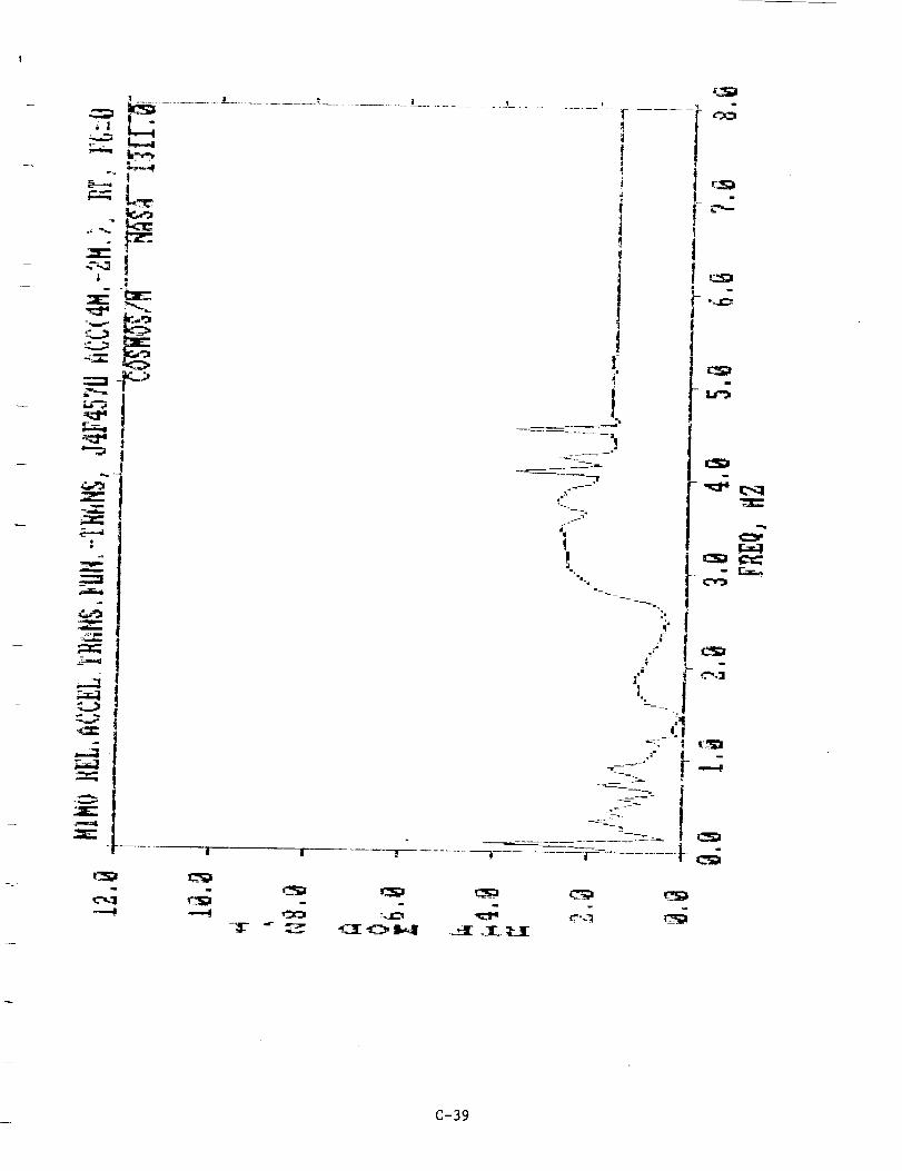
E,_" ! -
,dllmlll
"IZl'=="ll
Z-.T..,]
z_",.3
111
m
r----
ii
|'I
I,I
I!I
!!'
I1%
.... _ ....... --zl
1
iJ'
'iI
! -
i-_..
!!
t..g
i
q
_.,!I
-:/:
_-----. |
t | r
C-39
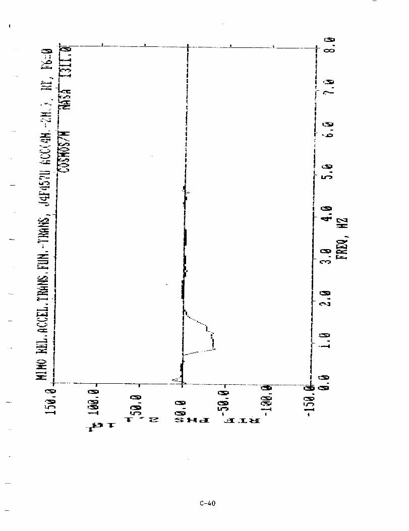
!
l|
_._ -
-- I
T I I L .......
-i_ -_T
r -_]5-
r_I
I
I|
t
!
_ -c L¢"_
%_ -
---,-4
!
C-40
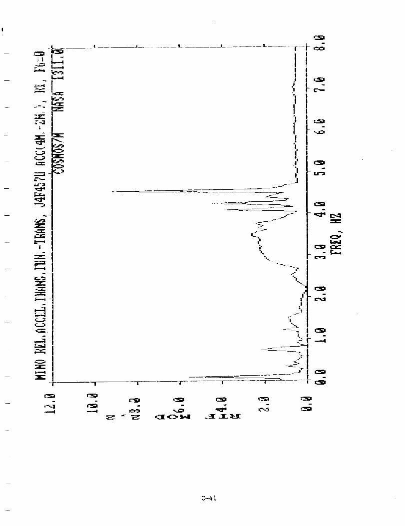
....-, ,_
I
nr'__
m
4.,6.,
0
if-
J.,,__......... .L......... r--t- ,_
*!|
"iI
]Ii,I!
.!
li
_-:__---
.2!._i-
I0°!
IwI
i.
|
"1
EI
!!I
i
i
_,.10
i
u
-=--I __= _
C-41
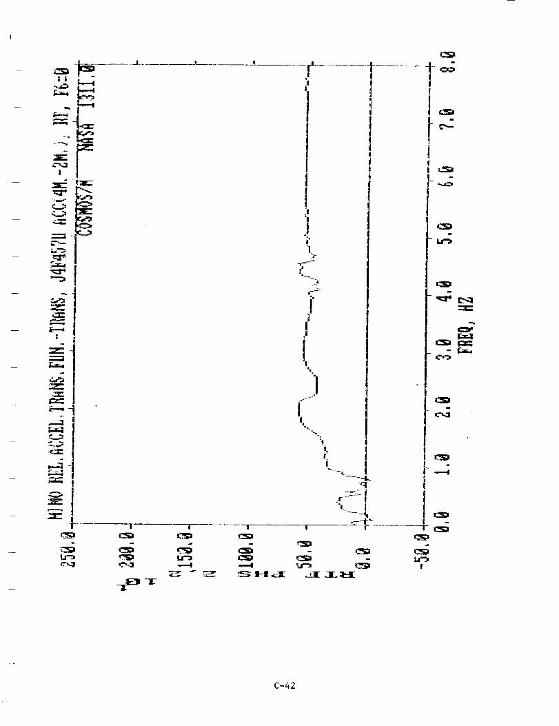
q
_.='L_ !
!
_E_
Lml
_1 _
|
| ! I
.r
!
|
II1
¢"---_
iiL.ii
II..
!i
!
-t
T
H .,_lE -.-1" -1"- :IE_
!|!
k.,=:
m
--,z,.,-
,=7!F-..x.,Z¢:z::
z:",-.i
m
z:",,,.1
i
!
!
C-42

.....7
E
Z
J
-!
.L_
n ! T 1
m
mc2_m
_Tr <I O _k_al
I"
q
t
L -
N
C-43

;| -
.
_" ..I_iE
--I
v
|
-i
| I
r
-_-w m
-_.__
.!
--_____
....._-LZ----_
.!
ol_
u--r
Ii
|d
-'1
i=.
|.u
.!
f
!Iii
Io
___
I.
J_
IlIi
I -
O
I!
I(
[!!
!
|
i
I i !
C-44

i,-....
a
Z
|
=E
_=K::I
i
{
!
i
JJ
iI
/I
L
I
L ............. -_
I ! IS I-I_l; _ _Ir_:I_I[
Ii
I
| t"--
ia
!
!
i
|
I
C-45

APPENDIX D
NONUNIFORM ENFORCED MOTION USING LARGE MASS METHOD

This appendix contains analytical calculations for the nonwniform
enforced motion problem for a simple tKree degree-of-÷reedom system. Two _f
the mass points <at Nodes i and 3) have correspondin@ desired enforced
accelerations. TKe third mass point (at Node 2) is between them and
undergoes dynamic response, it is shown that the large mass method of
nonuniform enforced motion work and that the fixed-base problem _r the
system can be solved.
D-2

t _ ENGINEERS, INC.
9937 Jeffe,son Boule,,ar,,n Currier Cb, CA 90232
_o___ h__Y o___ _I/_/t_..CHECKED BY ___ DATE 3!"_-I/,_"
JOB NUMBER
DESCRIPTION
PAGE / OF___
J
/Hz =
CM3 =
[/_ 1{_') + [_1[,} - [r}
"_t _ o o
o lvt o
o o /4_'
r"
/(I -Kj o
0 -/_L KZ
l[K.7 = KI -I 0
-I 2. -I
o -I _d
D-3

__O ENGINEERS, iNC.
9937 Jefferson Bou_evarn Curve, C_tv CA 90232
CHECKED BY DATE . 5]_'/eJ _"
,OB,OMBE, ,AGE 2.. OF_____
K--- t,u_',4,'t_ : O 6,o -
. ° =
'2.."-0
I]-4
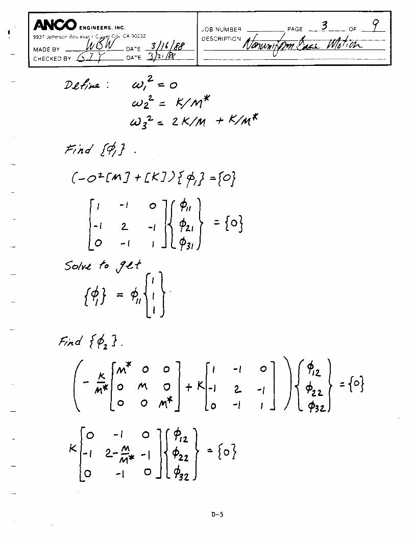
!__ll_ ENGINEERS, INC.
9937 JePerson Bouleva_/_Jv CA :)0232MADE BY DATE
CHECKED BY _fj7 F DATEI
JOB NUMBER PAGE 3 OF
DESCRIPTION • /" _ _ ..,,n /,
2.
Z" -- z/<7,_ -I-
C-.o'-C,_.7, cK.19f p j
- J{I -I o I (p.
-I 2. -I _""
0 - I I wZ!1
So/v-_ /',, J_'/"
r,.z __.
°°] [_:-'.. _,°]/r 1_0 /1,1_: -i
/<0 -I 0
-i 2--_4, -I
0 -I om
_. -_o}I,.%J
D-5
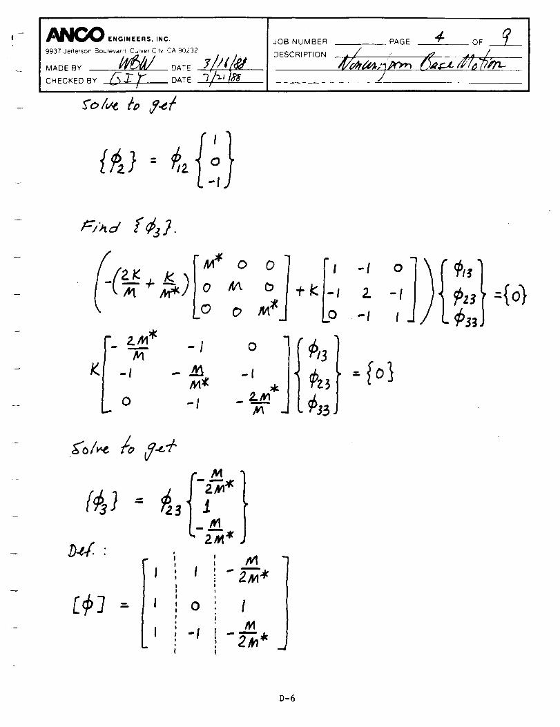
I _ ENGINEERS, INC.
9937 Jefferson Boulevard Culver C,lv CA 90232
MADE BY _/_._ DATE
JOB NUMBER
DESCRIPTION
_2PAGE OF---L--
./ _ ,_ ..,/4/_.'_.m',_ (_,_,_',_--
Y
{'t-'1
Jl_ f
I " I " ", ; _'-_'4eI ',
ccJ ' ' ,= I I O :
I _ -I
D-6
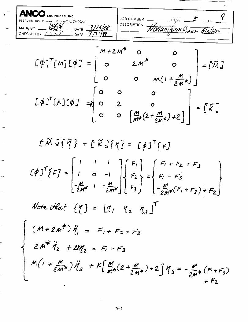
_NCO ENGINEERS, INC.
90232
JOB NUMBER
DESCRIPTION
b/
o
L_3T_3C_3 =t
" _ "1"2.,_ _ 0 0
0 2-_ _ 0
/I,1o o _(, +_--/,)
,m
0 o 0
0 2. o
I I I
I o -I
FI "1
I. _3j - _'Z F, + _'3) + Fz.
• j-r('(} - L¢, ,_ %
D-7

I _ ENGINEERS, INC.
9937 Jelterson Boulevarcl Cul r C_ CA 90232
i
JOB NUMBER
DESCRI PTION A/_ ,/ ....._ ..,I
IV_ __p,,6ore+_J_6_Lill,,__,-5,"#7'---
_'_ (/'_""J '7:
AI_ /14_ >>_ /_t
D-8

_J__ ENGINEERS, INC,
_.,,..e,..=ou,__,,__._o...h It."MADE BY DATE _'
JOB NUMBER
DESCRIPTION
PAGE ? OF __._
/I ' _./
2_... | 3
¢
/
(7
D-9

m
i__O ENGINEERS, INC.
9937 Jefferson Bouievaf_ Culve_ C_Iv CA 90232
MADE BY _//6_'_/" DATE
CHECKED BY _ "_ ! OATE
libw
JOB NUMBER PAGE
DES CRI PT 'O N _"Z_j,,/ _'t_/;i;, ,/_::_.;.._1,1_,
' __)
oe
__r'_ /'/ /3- S.t.._
_,,/_. 7-//_,5
J
m,...=.,
w
D-tO

_lC_O ENGINEERS, INC.
9937MADEBYJefferson Bou_ar,q_Culver/a_/C'tv CADATE902323h_/£t
JOB NUMBER PAGE
DESCRIPTION '_/_P"f/'_/g/_"_
I'}o'{U, l!
/
o jLJ-}=== _<-".,"-.
D-it

m
APPENDIX E
DERIVATION DETAILS FOR A DAMAGE INDICATOR

!
TKis appendix contains the derivation of one of the 9eneral damage
ndicators and an example of a specific case of it.
E-2
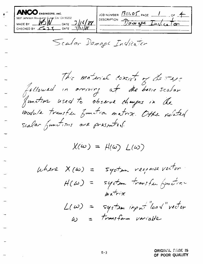
ii __////_ ENGINEERS, INC.
9937 Jefferson Bou_ _ City CA 90232MADE BY . • DATE
CHECKED BY _,,.. "3. "_ DATE-- t
JOB NUMBER
DESCRIPTION
/31p,or" PAGE I o_
V
._-q jot
=
Lo 9
l
/
/ /
_ _._ I'_, _
E-3 ORtGI_;._L ?,.:_GEIS
OF POOR QUALITY

I_IN_ ENGINEERS, INC.
9937 Jefferson Bout.e_er City CA 90232
MADE BY /_. _ DATE
CHECKED BY ___ DATE
JOB NUMBER
DESCRIPTION
t3ft,_Y%AGE 2-- O, _L
7.),_,,.,_r...eJ.__,o','c r.,..Tc..f-U
/__"/ /7- _°- + a/-/
X' - (6 °- + 4/--/_ L = /-/°L + 44 L
/
"b,-,;,>-,_. o,.,-1,."9,,.-/ ,..,_d-o,,-<m
+ L
O<'_4('i:;i,.,. ., 7.: !,.,
OF POOR (._q,':LLTTf F:-4
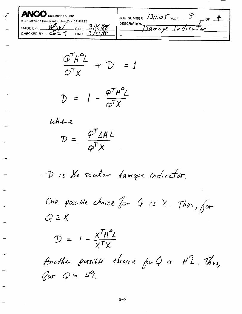
__B_ ENGINEERS, INC.
9937 Jefferson Boulevarrt Culver.,C_tv CA 90232
_o_.0,.,_,_,/3//. o r"PA_ 3' o_!
r _3-o,,,-
'D =" I -
J'b

I 1
JOB NUMBER
DESCRIPTION
Lr#oT#oLLT_oT×
g-6

APPENDIXF
CASESTUDYUSINGTIMEDOMAINSYSTEMIDENTIFICATION

| i--
This appendix contains exerpts from a published paper by Dr. J.L. Beck.
it provides some of the details of the theoretical aspects of his time
domain system identification approach to obtaining module modal promerties.
It also provides a case study where his method was successfully used to
obtain tNe desired mode mromerties.
TNis appendix also contains material on the lack o+ identifiability _n
determinin9 a pseudostatic matrix for a £eneral module of a system.
F-2

EARTHQUAKE ENGINEEI_ING AND STRUCTURAL DYNAMICS. VOL. !5, 249-274 O987_
SEISMIC RESPONSE EVALUATION OF MELOLAND ROAD
OVERPASS USING 1979 IMPERIAL VALLEY EARTHQUAKERECORDS
S D WERNER
Wis_. Janncy. Elstner As_ooates. Inc. 2200 Powell Street. Suite 925. Emcryville. California. USA
AND
J L. BECK AND M B. LEVINE
Earthquake Enginterin¢ Re,arch Laboratory. Californm Institute of Technology. Pasadena. Californm. US.A.
SUMMARY
During the 1979 Imperial Valley earthquake, an array of 26 strong.motion accelerometers produced records for theMeloland Road Overpass, a two-span reinforced concrete bridge structure located only 0-5 km away from the causativefault for this earthquake event. This paper describes the application of a new system identification methodology to the arrayof strong-motion measurements, in order to assess seismic response characteristict of this bridge. Results of this applicationshow that (1) linear models provide an excellent fit to the measured motions of the bridge, despite the fact that it wassubjected to very strong shaking; (2) the transverse response of the structure is controlled by its abutment motions, with nosignificant dynamic amplification in the deck, and [3) the vertical response of the bridge deck at the midlength of its Sl3ansisdominated by a single vertical translational mode wheremt, above the central pier, the deck's vertical response is mostaffected by the vertical motions of the pier base and by torsion of the deck. Also, systematic estimates of modal dampingratios and qualitative assessments of states of stress developed in the bridge during the earthquake are provided.
1. INTRODUCTION
I.l. General background
Bridges are important elements of lifeline systems, providing for the transportation of people and materialsacross man-made and natural obstacles.It is important that bridges maintain this function following a major
earthquake so that they do not impede either disaster relief or the long-term economic recovery of the affected
area. The ability of bridges to withstand strong earthquakes is therefore a topic of considerable concern both to
engineers and to public officials.
Past earthquakes have often caused extensive damage to bridges, resulting in significant economic loss,inconvenience and hardship to the surrounding communities, t-' Because of this, seismic design and
retrofitting provisions for bridges in the United States have been substantially upgraded in recent years,particularly since the 1971 San Fernando earthquake, s-t2 In addition, there has been significant activity
among earthquake engineers directed toward gaining further insight into the behaviour of bridges during
earthquakes. These activities have entailed quafitative observations and interpretations of the behaviour ofbridges during past earthquakes, 13-Is analytical research programmes that have investigated how the seismic
response of bridges is influenced by non-linear response phenomena, travelling wave effects, skewness,soil/structure interaction, etc., re-t9 and experimental research involving dynamic testing of bridge com-
ponents, 2°-2_ shake table tests of bridge models, '3 ambient vibration measurements of actual bridgestructures, 2a'25 and full-scale forced vibration tests of bridges. 2e'27
In addition to the above research activities, it is clear that strong-motion measurements of actual bridge
response, when obtained from a well-planned array of instruments and evaluated using established system
0098-8847/87/020249-26513.00
1987 by John Wiley & Sons, Ltd.
Received 2 October 1985
Revised 9 May 1986
F-3

I
250 S. D. WERNER, J, L. BECK AND M. B. LEVINE
identification techniques, can also provide important quantitative information concerning the seismic response
of bridges. However, to date, only five bridges in the United States (all in California) have been instrumented torecord earthquake motions according to established guidelines and procedures. 2s-3° Of these five bridges,
three have yielded significant earthquake response data, but only two of these bridges have been studied using
system identification techniques, za'3' As shown in this paper, such data can indeed provide valuable insightinto the seismic behaviour of bridges.
1.2. Bridge description and study ouer_,iew
In October 1979, the Imperial Valley earthquake (magnitude 6..4) occurred along the Imperial fault, with
rupture initiating just south of the United States-Mexico border and propagating in a north-westerly direction
along the fault [Figure. l(c)]. Significant shaking was produced throughout southeastern California andnorthcentral Mexico and numerous strong-motion records were obtained, particularly in the near field? 2-a4
Among the accelerograms obtained during this earthquake were those measured at the Meloland Road
Overpass (MRO), a reinforced concrete bridge structure located east of El Centro, California. The MRO iscomprised of two 104-ft spans with box gorder construction, monolithic abutments and a single-column central
pier [Figures l(a) and l(b)]. Because of its close proximity to the Imperial Fault [Figure. l(c)], the MRO had
previously been instrumented with an array of 26 strong-motion accelerometers along its deck, at its abutmentsand embankments, at the base of its central pier, and at a nearby free-field location (Figure. 2). All of these
instruments were triggered during the Imperial Valley earthquake, providing the most extensive array of strong-
motion measurements yet obtained for bridges in the United States. It is noted that the MRO wu virtuallyundamaged by the earthquake? s'3s despite the intense shaking to which it was subjected (0-51 g
transverse acceleration measured on its deck).
This paper describes results of a study that evaluated this important array of data in order to obtain insights
regarding the behaviour of bridges when subjected to strong seismic excitation. The study consisted of threemain parts that entailed (1) a reprocessing of the original strong-motion data in order to circumvent certain
recorder-induced distortions of the records; (2) development of a new system identification methodology
suitable for evaluation of this extended array of bridBe respons_ data; and (3) application of the methodology tothe reprocessed data in order to evaluate the seismic response characteristics of the MRO? l
2. STRONG-MOTION DATA REPROCESSING
2.1. Instrumentation
The MRO was instrumented in November 1978, about I l months prior to the Imperial Valley earthquake..
This instrumentation (Figure. 2) consists of two 13-channel remote-accelerometer central-recording systems• It
comprises FBA-1 (single-axis) and FBA-3 (triaxial) force-balance accelerometer packages, two 13-channelcentral recording units interconnected for common timing and a triggering system• The recorders and trigger
are located at the ground level next to the base of the central pier. The FBA accelerometers have a natural
frequency of about 50 Hz and are designed to measure accelerations up to I g over a nominal frequency rangeof O to 50 Hz; 3s The bridge instrumentation system is maintained by the California Division of Mines and
Geology, Office of Strong Motion Studies.
• .4
• 4, the MRO during the Imperial Valley earthquake are shown in Figure 3.•_ _hannel accelerometer systems operated during the earthquake,
--,_rder for Channels l-to- 13, which led to data loss- ',_otions from the two recorders was
_-_ing to correct for these
F-4OF POOR QUAL!W_.,

lip
(a) View lookinll east
2011' 34'
I '°* '°* t F lAIIIt. I le_t | AIV_ )
ELEVATION
(b) Bridlle dimensions
TYPICAL SECTION
_lq I"
t IS'I" 119"31"
(c) Proxanuty to Imperial Fault
Figure 1. Bridge configuration and location
ORIGINAL P.::C;_" IS
OF POOR QUALITY
F-5

N _ / ' -_ /_IMTERSTAT[_ / /
/_,_/"_ *OuTtO -'-/ / /
.ELOC_U_O s'muc'ru*x .. . (_) .- . /,,v,"/
• ACCEbERGGRAP)I ¢NOJMEI. NUI_ER : • _PREE-FIELO ACCELEROGE/U) ItANrdq[ T
- _ mOTION j_pr/ / _. jt"p_ / ALONG lalE01AI_ STRIP)"
I, i " ' " l . . :/ /SCALE (_IIT)
Figure 2. Meloland Road Overpau strong motion instruments
original film traces were reprocessed at the facilities of the University of Southern California. This reprocessing
incorporated (1) new digitization techniques and software that were specially developed to correct theacceleration and time coordinates of the distorted traces; and (2) standard corrections for instrument frequency
response and baseline adjustment? i The end result of this process was a set of uniformly processed time-
history records, together with Fourier and response spectra from each of the 26 channels of data obtained at the
MRO (e.g. Figure 4).The recorder non-synchronization problem was identified by computing the cross correlation between
several pairs of MRO acceleration records. The records that comprised each pair were typically each from adifferent recorder, and were measured at locations whose motions should be well correlated except for
recorder-induced non-synchronization effects. Results of this assessment showed that the motion from theChannel l-to-13 recorder consistently led the motions from the Channel 14-to-26 recorder by about 60 rnsec.
This was corrected by an appropriate time shifting of the motions from Channels 1 to 13.
3. MODAL IDENTIFICATION METHODOLOGY
3.1. Theoretical basis
To evaluate the array of records measured at the MRO, a new modal identification methodology was
developed. This methodology, named MODE-ID, is applicable to an elastic system with an arbitraryconfiguration, with classical normal modes, and with motion measurements from any number of input and
system response degrees of freedom. It is also assumed that the system is initially at an at-rest position.
The MODE-ID methodology considers a vstem whose equations of motion are
[M] {?}+[C] {t'}+[g] {r) = -[C,d {Z}-[K,f] {Z) (I)
where
[M], [C], [K] = mass, damping and stiffness matrices of the system
{ Y} -- vector of motions at N system degrees of freedom{Z} = vector of input (support or 'foundation') motions at NS degrees of freedom
[C,f], [Ksr ] = damping and stiffness matrices that couple the system and 'foundation' response.
Following procedures de:cribed by Clough and Penzien, 36 the acceleration of the system is expressed as
{?} -- {S} +{X} (2)
F-6

where {_I and IX} are the pseudostatic and dynamic components of acceleration respectively. In this, the
pseudostatic component represents the 'static' contributions of the individual support motions to the systemresponse (neglecting inertial and damping effects), and can be visualized as a time.<lependent 'reference'
position of the structure whose deformed shape at each instant of time is dependent on the instantaneous
position of the structure's supports. This pseudostatic response is expressed as
= (z} (3)
where [/_] is the pseudostatic matrix, given as
[/_] : - [K]-t CKsr] (4)
The dynamic component shown in equation (2) represents the contributions of the system's fixed-base modal
vibrations about its pseudostatic reference position. The equations of motion for the dynamic responsecomponent ate obtained by substituting equations (2) to (4) into equation (1) and neglecting the contributions
of damping to the effective earthquake forces) 6 These equations take the form
[M] Ix)+[c] {x} +[t:] {x} = -[M] (5)
In order to get a realistic spatially discrete model for the bridge of the form described in equations (1) to (5),
the total number, N, of structural degrees of freedom would normally be chosen to be much greater than the
number, NR, of structural degrees of freedom at which the response is actually measured. As a consequence, it
is not possible to determine uniquely the elements of the stiffness and damping matrices from the measuredseismic excitation and response, even if the mass matrix is assumed known. 37 Instead, an identifiable model in
which the parameters are uniquely specified by knowing the excitation and response may be derived byassuming classical modes of vibration, as presented in the following discussion.
Let st and xl, i = 1, 2 ..... NR, denote the pseudostatic and dynamic components of the response at the NR
degrees of freedom at which the system response is measured. The pseudostatic components s_can be obtainedfrom equation (3) using an NR x NS submatrix [R] of the full N x N5 pseudostatic matrix [/_]. Also, the
dynamic components x_can be expressed as the superposition of the contributions of NM modes of vibration
of the system which are significantly excited by the earthquake (NM 4 iV). This is expressed mathematically as
NM
x_(t) = _ xt,(t) (6)rm|
where x_, is the rth mode response of the system at its ith degree of freedom. From a modal decomposition ofequation (6) that incorporates orthogonality of the mode shapes, it can be shown that the modal contributionsx,,, i = 1, 2..... NR, satisfy the equation:
{x_} + _,{ _,,1 + b,{x_,} = -[ P")] {_.} (.7)
where
a, = 2_,_,
b, =
_,, % -- damping ratio and natural frequency respectively of the rth mode,
and [ P_')], the effective participation factor matrix for the rth mode, is expressed as
CF.,)] : [p:;,] :0_,_',, _:,y,_
%,,,I(8)
In this, 0_, is the mode shape amplitude ofthe rth mode at the ith degree of freedom (i : 1,2 ..... NR), and 7,j isthe conventional participation factor of the rth mode for thejth support degree of freedom (j = 1,2 ..... NS).
F-7

The ;% are elements of the matrix.
Erl = [;,.1 = [¢]TI'M] [R] t9)
where [_] = [_i,] is the mode shape matrix. It is seen from equation (8) that thejth column of[/_')] contains
the common factor "Aj. Therefore, once [ P')] is obtained, the mode shape for the rth mode can in theory be
readily calculated as the ratio of the elements in each row of any of the columns of [p4,,]. However, thesecalculations are ill-conditioned when the various support motions are nearly identical, which is the case t'or theM RO. 3t Therefore, for such conditions, it is more desirable to obtain the mode shape from the ratios of sums
of the rows of r p4,)]. This ill-conditioning is discussed further in Section 3.3.
3.2. ldentificatwn procedure
The above discussion shows that the pseudostatic matrix [ R], and the normal mode parameters a,. b, and
[ P'_], (r = 1.2 ..... NM) represent the complete set of parameters needed to fully characterize the system'sresponse as its measured degrees of freedom when it is subjected to the measured input motions. In MODE-ID.
an optimization procedure is applied to estimate these parameters, in which the following error function is
minimized:
I NI_ NT
t0>J (O) = -_ ,. ,-o
where
ffi, Yi= measured acceleration and model acceleration at the ith measured response degree of freedom
At -- sample interval of the digitized accelerogramsNT = total number of time samples (at interval At)
0 -- modal parameters to be estimated
= {CR]; a,, b,, CP_"]: r -- 1,2 ..... NM}
and V is a normalizing factor given by
Nil NT
V= _. _ _(nAt) (ll)
Therefore, J may be interpreted as the ratio of the mean-square error in the model acceleration to the mean-
square of the measured acceleration.
The minimization of J with respect to the model parameters is implemented in MODE-ID using an iterative
algorithm that is an adaptation of the modal-minimization method developed by Beck) 7 This algorithmconsists of a series of modal sweeps in which, during each sweep, the estimates of the elements of the
pseudostatic matrix [R] are first updated by minimizing J with respect to these elements only. Then, the
estimates of the parameters of each mode (a,, b,, [/_"]) are successively updated by a series of sinsle-modeminimizations of J. This minimization for each mode actually corresponds to least-squares matching of a
modified measured response in which the contributions of the pseudostatic response and the other modes are
subtracted out; these contributions are computed from the new parameter estimates for those modes already
treated in the sweep, and from the prior parameter estimates for those modes not yet treated. A single sweep iscompleted when the pseudostatic response and all significant modes have been treated in this manner.
Successive modal sweeps are performed until the fractional decrease in J is less than a prescribed value, or until
a prescribed maximum number of modal sweeps has been completed.
F-8

Usually only the first one or two of the strongest excited modes selected from the Fourier amplitude spectra
of the records are initially included in the optimization process. Additional modes are then added, one at a time,
by choosing appropriate initial estimates for the natural frequency and the damping ratio. Successiveoptimizatiorls are performed until it is judged that all modes that significantly affect the response have been
included. The modes are added successively in this manner so that it is easier to observe whether or not a mode
has a significant effect on the match of the measured response.
In performing the minimization of J for each mode, the effective participation factors ,,jd"_,_li-- I, 2, .... NR;.j = I, 2..... NS) are treated as being independent. This is not strictly correct since certain auxiliary conditions
must be satisfied. 3t For example, the mode shapes derived from the effective participation factor matrices
should satisfy the orthogonality conditions. These auxiliary conditions on the PI_'are not enforced since theyinvolve the complete mode shape and pseudostatic matrices, whereas only those submatrices corresponding tothe measured response degrees of freedom are actually estimated from the data. Therefore, the model used in
the identification process may be viewed as being more general than the classical normal mode model described
above. However, if the assumptions inherent in a classical normal mode model are sufficiently accurate, thenthe auxiliary conditions should be satisfied automatically by the estimated d"
•:ij "
3.3. Effects of nearly identical support motions
The development provided in Sections 3.1 and 3.2 applies to the general case of any arbitrary input motions
measured at each of the NS support degrees of freedom of the system. However, inspection of Figure 3 shows
that the recorded 'support' motions of the MRO at the abutments, embankments and pier base in a given
direction are nearly the same. Therefore, it is appropriate to consider the equations of motion for the limitingcase where the support motions in a given direction are identical.
The vector of support accelerations may be expressed in this 'rigid-base' case as
{2(0) = z_r_t){It} + _v(t) {zv} (12)
where _t and Z'v are the common accelerations of the transverse and vertical support degrees of freedom
respectively; {It} is an N5 × l vector whose elements are unity and zero corresponding respectively to
transverse and vertical support degrees of freedom: and {I v } is an NS x 1 vector whose elements are unity andzero corresponding respectively to vertical and transverse support degrees of freedom.
Using equation (12), equation (3) becomes
{S(t)}-=[_] {zTl_(t)+[R] {iv} _,(t) (13)
showing thatthe pseudostaticresponseiscontrolledby the two N × I vectors
(14)and {sv} = [/_] {Iv}
and not by the values of the individual elements of the pseudostatic matrix [/_']. From equation (14), each
element of the vectors {st} and {Sv} is equal to the sum of the elements in the corresponding row of [/_],
summed over the transverse and vertical support degrees of freedom respectively. Furthermore, because {s,r}represents the system's static response to unit rigid-body translation in the transverse direction, its elements are
unity and zero, corresponding respectively to transverse and vertical response degrees of freedom. Similarly,since {sv } represents the system's static response to unit vertical rigid-body translation, its elements are unity
and zero, corresponding respectively to vertical and transverse response degrees of freedom.
In a similar manner, substituting equation (12) into the right-hand side of equation (7) leads to
- [_"] {_} = - [_"] {J_)_T- [_"] {_v}_v (_s)
showing that the excitation of the rth mode contribution to the system's dynamic response is controlled by thetwo NR × 1 vectors
{_"}= [P")]{h}(t6)
and {p_')} = [P(')] {Iv}
F-9

¢and not by the values of the individual elements of the effective participation factor matrix [P_')]. Fromequation (16), each element of the vectors {_')} and {/_")} is equal to the sum of the elements in the
corresponding row of [P_')], summed over the transverse and vertical support degrees of freedom respectively.From this, it can be shown that
{_')} = ,:_') {¢(') }
(17)and (_')}--7_v"'{c/,"'}
where {O(') } is the NR x 1 mode shape vector of the rth mode for the measured response degrees of freedom,and the scalars-/T(') ",,-'="'4Yv(') =,-_"the conventional rigid-base participation factor for the rth mode in the transverseand vertical directions respectively.
The above discussion shows that the parameters controlling the response of the model when the supportmotions in a given direction are identical are {s r }, {Sv} and the parameters {_') }, {p_') }, _, and (, for each mode.
Itfollowsthatitisonly theseparameterswhich can be determined uniquelyduringtheapplicationofsystem
identification,usingthemeasured common support motions _Tand _vtogetherwith the measured response.
The individualelementsof the matrices[R] and [/_')]are not identifiable.Ifthe support motions in each
directionarenearlyidentical,asintheMRO, thentheelementsofthesematricesmight be identifiableintheory,
but inpracticethe estimationprocessisill-conditionedbecauseof the presenceof measurement noiseand
model error.The aforementionedparameterscontrollingthemodel responseshould,however,stillbe reliablyestimated.
Inview ofthisill-conditioning,themode shapesforMRO were evaluatedusingequations(16)and (17),that
is,the elements in each row of the identifiedeffectiveparticipationfactormatrix were summed over the
transverseand verticalsupport degrees of freedom separately.This gave the transverseand vertical
components respectivelyof the scaledmode shape vector.Also,the elementsin each row of the identified
pseudostaticmatrix were summed over the transverseand verticalsupport degreesof freedom separatelyto
compute the vectors{sT}and {sv} inequations (14).These vectorswere then checked to assurethattheir
elements were closeto the theoreticalvaluesof zero or unity.
As a finalremark,ifMODE-ID were appliedto a long bridgewith markedly differentsupport motions
becauseoftravellingwave effects,then theabove ill-conditioningwould not occur.Inthiscase,theindividualelementsof fR] and [P("] should be estimatedreliablyby MODE-ID.
. 4. OVERVIEW OF SEISMIC EVALUATION PROCESS
The evaluationof the MRO's seismicresponse was comprised of two main stepswhich involv,-_'
assessment of the MRO's modal and seismic response characteristics; and (2) applicati,--arrays of the MRO's measured strong-motion records. In performing the,," "
essential element in the proper application of the system identificati,--more fully by Werner at al. a t
4.1. Initial assessment process
An initial _ment of o-
lD applicatio.-"
F-IOORI_NAL P._E IS
OF POOR QUALITY

5. BRIDGE RESPONSE CHARACTERISTICS
The above seismic evaluation process was applied to two subsets of the MRO's vertical and transverse strong-
motion records, in order to assess dynamic response characteristics of two alternative subsystems of the bridge.
Results of the MODE-ID application to these two subsets, denoted as Case 1and Case 2, are summarized in the
paragraphs that follow.
5.1. Case 1 results
The Case 1 subset of MRO records consists of input records which are the transverse and vertical motion
measurements at the two abutments and the central-pier base, and response measurements which are the
transverse and vertical motion measurements along the road deck (Figure 5). Therefore, this subset emphasizes
the dynamic characteristics of a subsystem consisting of the road deck and central pier. whose contributions tothe total bridge response are represented through the fixed-base normal modes that are identified. The
pseudostatic matrix identified in the Case 1 application represents the additional 'quasi-static" contributions ofthe abutments, embankments, central-pier foundation, and underlying soil medium to the overall bridge
response.This Case 1 application resulted in the identification of a pseudostatic matrix [R], and two normal modes.
The identified matrix JR1 is not reported here because of the ill-conditioning that arises from the near
N
LEGEND :
'--1,, INPUT CHANNELS
n RESPONSE CHANNELS
Figure 5. Cax I: input and response charmer-
coincidence of the MRO's support motions in a given direction (see Section 3.3). However, the sums of theelements in each row of [R] were close to their theoretical values of zero or unity. 3t It is these sums which
control the pseudostatic response of the bridge because of the nearly identical support motions.The two normal modes that were identified have the characteristics shown in Table I. The first of these
modes, termed the deck vertical mode, has a natural frequency of 4.7 Hz, a damping ratio of 6_ per cent, and amode shape consisting of vertical translations of the two deck spans that are nearly symmetric about the central
pier. The other identified mode, termed the deck transverse mode, has a natural frequency of 3.7 Hz, a dampingratio of 6_ per cent that by coincidence is virtually the same as that of the deck vertical mode, and a mode shape
consisting of transverse horizontal translations and torsional rotations of the bridge deck.
The degree to which the resulting bridge model comprised of the above two modes and the pseudostaticmatrix, represents the seismic response characteristics of the bridge is demonstrated by (1) the very low value of
the measure-of-fit parameter (J = 0-056) that was obtained; and (2) the very close comparisons that resulted
between measured motion time histories at various channel locations and the time histories computed at theselocations using the identified model (Figure 6). These show that the linear model that was identified has
produced an excellent representation of the seismic response of the MRO, despite the fact that the MRO was
subjected'to very strong shaking.
F-If

Further insight into the nature of the MRO response is provided through a series of comparisons of
measured and model motions at selected channels, as the contributions of each element of the model (i.e. the
pseudostatic matrix and each normal mode) are successively incorporated into the computation of the model
motions. Such comparisons are provided in Figure 7 for the transverse response at the midlength of the bridge(Channel 7), the vertical response at the midlength of one of the deck spans (Channel 16) and the vertical
response of the deck face above the central pier (Channel 2 l). These comparisons show that each element of the
MRO has affected its seismic response in a different way, as summarized below.
(a) The pseudostatic response, by itself, provides an excellent fit with the measured transverse motions of
the bridge; the additional contributions of the deck vertical mode and transverse mode to this fit aresmall [Figure 7(a)]. This shows that the transverse response of the MRO is controlled by the motions of
the abutment and foundation supports. The structure provides only slight dynamic amplification ofthese transverse support motions.
(b) For the vertical motions at the midlength of the deck spans, the principal contributor to the fit between
measured and model motions is the deck vertical mode [Figure 7(b)]. This single mode dominates thebridge's vertical response at these span midlength locations, and the additional contributions to this
response of the support motions (included through the pseudostatic matrix) and the torsional motions
of the bridge deck (incorporated through the deck transverse mode) are small.
Table 1. Case 1: significant modes of vibration
Mode Frequency* Damping Mode shape(Hz) ratio
Deck vertical 4.74 0.066(5'!2)
\ '0
Deck transverse 3.72 0-066(3.34)
• The values m parenthesesare those obtained from a simple finite element model ofMRO using equivalent rotational spring stiffnesses obtained from a simplebridge-foundation interaction model.)*
(c) For the vertical motions at a face of the bridge deck above the central pier, the deck vertical mode has a
node. Therefore, as shown in Figure 7(c), the primary contributors to the deck vertical response at thiscentral pier location are the vertical support motions at the central pier base (represented through the
pseudostatic matrix) and the deck torsional motions (incorporated through the deck transverse mode).
F-12
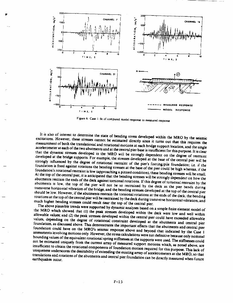
z
iO
m
,7.,.0,o
2OO
_00i
0
tOO
200
0
,_ CHANNEL 7
,//
2 4 6 I I0
TIME, $
v_
Z
Z
0
¢g
20C
_00
-_Oq
-200
0
CHANNfL t&
2 4 6 I 10
TI M Et $
z"O
Z
TOO , , , ,
TIME, S
_ _--.--_ --"_ -- ." "- 7------" :
...... MEASURED lit I SPON SE
MOOEL RESPONSI
Figure6. Caseh fit of computedmodelresponseto measuredresponse
It is also of interest to determine the stateof bending stressdeveloped within the MRO by the seismicexcitations. However, these stressescannot be estimated directly since it turns out that this requires themeasurementof both the translational and rotational motions at each bridge support location,and the singleaccelerometerateachof the two abutmentsandat the central pier baseis insufficientfor this purpose.It isclearthat the dynamic stressesdeveloped in the MRO will be strongly dependent on the degree of restraintdevelopedatthebridgesupports.For example,thestressesdevelopedatthebaseofthecentralpierwillbe
stronglyinfluencedby thedegreeof rotationalrestraintof thepier'sfooting/pilefoundation;i.e.ifthefoundationisfixedagainstrotationsthebendingstressesatthebaseofthepiercouldbehighwhereas,ifthe
foundation'srotationalrestraintislow (approachingapinnedcondition),thesebendingstresseswillbesmall.At thetopofthecentralpier,itisanticipatedthatthebendingstresseswillbestronglydependenton how the
abutmentsrestraintheendsofthedeckagainsttorsionalrotations.Ifthisdegreeoftorsionalrestraintby theabutmentsislow,the top of thepierwillnot be so restrainedby the deck as the pierbends during
transversehorizontalvibrationofthebridge,and thebendingstressesdevelopedatthetopofthecentralpiershouldbelow.However,iftheabutmentsrestrainthetorsionalrotationsattheendsofthedeck,thebending
rotationsatthetopofthecentralpierwillberestrainedbythedeckduringtransversehorizontalvibration,and
much higherbendingstress_couldresultnearthetopof thecentralpier.
The aboveplausibletrendsweresupportedbydynamicanalysesbasedon asimplefiniteelementmodeloftheMRO which showed that(I)thepeak stressesdevelopedwithinthedeck were low and wellwithin
allowablevalues;and (2)thepeakstressesdevelopedwithinthecentralpiercouldhaveexceededallowable
values,dependingon thedegreeof rotationalconstraintdevelopedat theabutmentsand centralpierfoundation,asdiscussedabove.Thisdemonstratestheimportanteffectsthattheabutmentsand centralpier
foundationcouldhaveon theMRO's seismicresponseaboveand beyond thatindicatedby theCase I
assessmentsinvolvingmotionsonly.However,thestresscalculationswerenotdefinitivebecauseonlynominal
boundingvaluesoftheequivalentrotationalspringstiffnessesattheSupportswereused.The stilTnessescouldnotbe estimateduniquelyfromthecurrentarrayofmeasuredsupportmotionswhich,asnotedabove, are
insufficienttoobtaintherotationalcomponentsoffoundationmotionrequiredforthispurpose."rh/slackofuniqueness underscores the desirability of extending the existing array of accelerometers at the MRO, so thattranslations and rotations of the abutments and central pier foundation can be directly measured when futureearthquakes occur.
F-13

6. CONCLUDING REMARKS
The results presented in this paper show that when seismic response measurements are obtained from a well-
planned array of strong-motion instruments and are evaluated using proven system identification methods,significant insight into the behaviour of bridges during earthquakes can be obtained. The results also show that,despite the intense levels of shaking that were involved, the classical mode models identified from the MRO'sstrong-motion measurements have provided a good representation of its seismic response characteristics.Other important practical results that should be useful in enhancing the future seismic design of bridgesinclude the following:
(a) Damping ratios. The results presented herein represent one of the first times that modal damping levelsattained in bridges during strong seismic excitation have been systematically estimated. Such dampingratios range from about 0.06 to about 0.08 for the various modes of vibration that were identified.
(b) Effects ofbridoe elements on seismic response. The relative contributions ofeach ofthe various elementsof the MRO (i.e. its abutments, deck, central pier, etc.) to its seismic response have been systematicallyisolated and evaluated. The abutments and embankments were seen to be the major contributors to thetransverse response characteristics of the bridge, whereas the deck structure dominated the MRO'svertical response characteristics. The torsional response characteristics of the deck/abutment system andthe bending response characteristics of the central pier also affected the transverse motions of the MRO.
(c) Dynamic stress levels. Qualitative evaluations and dynamic analysm using simplified models were usedto provide insights into the nature of the dynamic stresses developed in the MRO during the earthquake.These evaluations indicated that the central pier may well have been quite highly stressed, whereas thedeck probably was not. They also show that the state of stress developed in the central pier is stronglyinfluenced by the degree of rotational restraint provided by the abutments and the central-picrfoundation. Unfortunately, the bridge stresses could not be estimated in a definitive manner because theearthquake-induced translational and rotational motions of the abutments and the central pier basecould not be uniquely determined from the single set of instruments deployed at these support locations.
The results presented in this paper suggest additional investigations to further enhance the information thatcan be obtained from motions measured by this array of bridge instruments during future earthquakes. First ofall, it has been shown that the abutments and pier foundations had a major effect on the behaviour of the MROduring the Imperial Valley earthquake. Therefore, effort should be directed toward obtaining further insightinto the behaviour of these foundation elements. Such efforts should include (1) extendiilg the array ofaccelerometers at the abutments and piof foundation so that their translations and rotations about three axescan be doeermined; (2) dynamic testing of the MRO abutment and pier foundation elements in order todetermine appropriate impedances; and (3)careful measurement of static and dynamic properties of the soils in
the embankments and underlying geologic layers in order to support interpretation of future strong-motionmeasurements and dynamic test results.
In addition to the above efforts directed toward increasing our understanding of the behaviour of the M RO'sabutments, pier foundations and surrounding soil med/a, future investigation of the overall seismic response ofthe MRO using identification of extended bridge models should also prove to be valuable. The future use ofnon-classical mode models and certain class_ of non-linear models should further extend the basic insightsprovided by the classical mode models used herein.
ACKNOWLEDGEMENTS
This paper was prepared under a research project carried out at Agbabian Associates (AA) when the first andthird authors were members of the AA staff. The project was funded through a grant by the National ScienceFoundation (Grant No. CEE-8111964), whose financial support is gratefully acknowledged.
The authors also acknowledge the contributions to various phases of the research of the followingindividuals: M. D. Trifunac, V. W. Lee and S. F. Masri of the University of Southern California: J. T. Ragsdaleand N. A. Kaliakin, formerly of the California Division of Mines and Geology; R. M. Coppolino of MacNeal-Schwendler; R. F. Scott of the California Institute of Technology; and J. H. Gates of the California Departmentof Transportation.
F-14

Lack of Identlfiabllity in Determining
Pseudostatic Matrix for a Module of a System
Let the system have N dof (degree-of-freedom) with
z (t)=
Let K =
I :
For each
displacement at if-hdof
set of system dof at time t defining boundary motions ofmodule, and
set of system dof defining monitored output of module.
e_ , we can write:
where SL(_) = pseudostlatlc response
- 2 xjl)where p = [ 1= ] is the pseudostatic matrix and where
&_.{_) = dynamic response due to flxed-boundary modes of module.&
For identification of P, we would like to estimate the "_(k by
least-squares matching of the monitored accelerations E i {i_] , y _E_[_ ,=I
is part of an iterative process in which the objective is to determine P
and the n_odal parameters for the module.)
We now show that for sufficiently many inputs, this procedure will not
work, primarily because the module boundary motions are not independently
produced (i.e., produced by an agency external to the system) but instead
are related through the dynamics of the system.
F-15
I
Suppose that only the system modes re P- contribute significantly to the
system response, then to a good approximation
: , V (" : l,Z,...,_/
..=-where 17 (_) is the modal acceleration, and
Suppose we can choose the and ke K , so that
Then,
_i(*) - ,._K_k_(_> ' V ieI.
That is, when attempting to identify the pseudostatlc parameters,
e0
erroneous values will be obtained which make_.'_,kXk.¢ equal to the totalkeK
response rather than just the pseudostatic response. But does a solution
of Equation F-1 exist for the _'k _
Equation F-1 is a linear system of equations for the p[ k involving IIJJKJ
unknowns and #ZII_I equations, where IAI denotes the numbor of
elements in set A. Thus, a solution (not necessarily unique) exists for
the PEk iflzIIKI_IZlIEI i.e.IKI)IEI. Thus, a solution exists if the
number of inputs is not less than the number of modes which control the
system response.
F-16

An alternative way of looking at this problem is that with_l inputs toam
the module, it is possible to match exactly up to I_<;_modes in _i_t)with
an expression of the form --'l_' __(_[t) , but, of course, the resultingk_K k
estimate of the _k's will in general be quite different from the true
pseudostatic parameters. Thus, for the COFSMAST module with 12 boundary
motions as input it is possible to match the contributions of 12 system
modes to the module outputs by a suitable choice of the _'k " It can be
seen that from Equation F-1,if the system is damaged outside the module,
the system mode shapes will change and so these "false" pseudostatic
module parameters will change in general.
F-17

_OO
APPENDIX G
MODAL STRAIN ENERGY DISTRIBUTION
METHOD SOFTWARE

This appendix
Oistribution Method
listings.
contains a note about
Computer Code and the
the Modal Strain Energy
correspondin9 source code
C,-2

MEMO
TO: WIllIAM k&ad_TON
FM : BLUE JOf'l_
OT: 27 FEB 87
RE: NA_ OA_ SOFTt_E--C_SEIDM
This is a written summary of the programs I hae generated to date that allow
assessment of damage using the MSEDM. I have included source listings of
all the programs and a 1.2 Mb floppy diskette containing the source programs
and the executables.
MOOSTRN - This program computes element modal strain energies for a simply-
supported beam due to bending deformation only. The user must input the
number of elements and modes to use. The output element modal strain
energies are contained in the file JJPIS.O0jJ. This file is a binary file,
D_MIO - This program allows the user to input damage parameters to be used
in damage assessment. Oamage parameters are input on a mode-by-mode basis.
The user also specifies the output file containing the damage parameters.
This output file is an ASCII file.
MOOSLIM - THis program performs the damage assessment based on the modal
strain energies and the damage parameters. The user must input the file
name containing the modal strain energies and the damage parameters. The
user also specifies the damage fraction (g> used in assessing damage.
Alternately, the user can select the option of summarizing the element
strain energies for a giuen mode. In either case, Output data is conta ned
in the file _JMODSLIH.DD'.
G-3

$NOFLOATCALLS
C
C PROGRAM MODSTRN - COMPUTE MODAL STRAIN ENERGY MODE BY _ODE
C
IMPLICIT INTEGER*2 (I-N)
DIMENSION XTRN(200) ,XAVG(20c))
CHARACTER*80 KEY
CHARACTER*40 TITLE
COMMON/XDAT/XTRN,XAVG
C
C CLEAR SCREEN,DISPLAY PROGRAM
C
KEY = 'MOD_TRN - F'ROGRAM TO COMPUTE MODAL STRAIN ENERGY
CALL VCLEAR
CALL VCURXY(O,O)
CALL PRMFT(KEY,I.00)
CALL GCURXY(IC,IR)
IR = IR + I
C
C GET USER INPUTS
C
F_EY = 'ENTER DESCRIFTION OF RUN : $'
CALL KEYBD(KEY,R,I,TITLE,_, (40),O,IR)
IR = IR + 1
KEY = _ENTER THE NUMBER OF ELEMENTS TO USE : $'
CALL KEYBD(KEY,R,NELM,A,2, (2) ,O,IR)
IR = IR + I
KEY = "ENTER THE NUMBER OF MODES TO USE : ;'
CALL KEYBD(KEY,R,NMODES,A,2,(2),O,IR)
IR = IR + 1
CALL VCURXY(O,IR)
C
C OPEN UP BINARY FILE CONTAINING DATA
C
OPEN(b,FILE='MS.DD',STATUS='NEW',
i FORM='UNFORMATTED')
WRITE(6) TITLE,NELM,NMODES
C
C COMPUTE STRAIN ENER@Y FOR 100 PTS FROM 0 TO i
C
XLM = 1.0 / NELM
NELMP1 = NELM ÷ I
XPI = 4.0 * ATAN(1.0)
C
C LOOP OVER NUMBER OF MODES
C
DO 100 IMODE=I,NMODES
XMX = O, 0
XCOFF = 1.0
DO 10 I=i,NELMPI
XL = FLOAT(I-I) * XLM
XS = FLOAT(IMODE) * XPI
XSN = SIN(2*XS*XL)
XTRN(I) = XCOFF * (XL/2 - XSN/(4.0 * XS))
I0 CONTINUE
C
C COMPUTE ELEMENT STRAIN ENERGY
C
DO 15 I=I,NELM
G-4

IF(ABS(XAVG(1)).GT. XMX) XMX = XAVG(1)
15 CON T INUE
C
C SCALE T0 UNITY
C
DO 20 I=I,NELM
XAVG(I> = XAVG(1) / XMX
20 CONT INUE
C
C NOW WRITE IT OUT
C
WRITE(b) (XAVG(I) , I=I,NELM)
1I)O CONT INUE
STOP
END
G-5

SNOFLOATCALLS
IMPLICIT INTEGER*2 (I-N)
DIMENSION DAM(20),DAMCRT(20)
CHARACTER*80 KEY
CHARACTER*bO DAMTTI_
CHARACTER*20 DAMFIL
CHARACTER*I IEDCR
C
C CLEAR SCREEN, ETC
C
CALL VCLEAR
CALL VCURXY_O,O)
_EY = DAMIO - FROGRAM TO CREATE/EDIT DAMAGE F ARAMETERS_ _
CALL PRMPT(KEY.I.00)
IR = 6
IR = IR + 1
KEY = DO YOU WANT TO (C)REATE OR (E)DIT A DAMAGE FILE? :
CALL KEYBD(KEY,R,I,IEDCR,3, (I) ,O,IR)
C
C HERE FOR FILE CREATION
C
CALL VCLEAR
IR = 0
CALL VCURXY(O,IR)
KEY = DAMAGE _ITLE : $"
CALL KEYBD(KEY,R,I,DAMTTL,3,(bO),O,IR)
IR = IR ÷ I
KEY = NUMBER OF MODES USED : $"
CALL KEYBD(KEY,R,NMODES,A,2,(2),c),IR)
IR = IR + 2
CALL VCURXY(O,IR)
WRITE(*,9010)
9010 FORMAT(1X,'MODE',5X,'D(W) ",fOX, Dcrit(W) '\)
IR = IR + I
CALL VCURXY(O,IR)
WRITE(*,9002)
9002 FORMAT(' NO. "\)
IR = IR ÷ 1-
C
C NOW READ IN DATA
C
IST = IR
IEND = IR + 9
DO 20 IM=I,NMODES
CALL VCURXY(O,IR)
IF(IR.EQ. IST) WRITE(*,9200) IM
IF(IR.NE. IST) WRITE(*,9201) IM
KEY = " $"
CALL KEYBD(KEY,DAM(IM),I,A,I,(10),9,1R)
CALL KEYBD(KEY,DAMCRT(IM),I,A,I,(IO),23,1R)
IR = IR + 1
IF(IR.LE. IEND) GO TO 20
DO 15 IERmIST,IEND
CALL VCURXY(O,IER)
WRITE(*,go00)
15 CONTINUE
IR = IST
20 CONTINUE
IR = 20
G-6

P
L.
C
C
GET OUTPUT FILENAME AND WRITE IT OUT
92(_ I
900()
8()0()
:3010
S020
KEY = 'ENTER OUTPUT DAMAGE FILENAME : _'
CALL KEYBD(KEY,R,I,DAMFIL,;, (20) ,(];,[R)
OPEN(5,FILE=DAMFIL,_TATUS= NEW')
WRITE(5,8000) DAMFIL,DAMTTL,NMODES
WRITE(5,8010)
DO 30 I=t,NMODES
WRITE(5,_O20) I,DAM(1),DAMCRT_I)
CONTINUE
FORMAT(IX,IX,13\)
FORMAT(I×,I3\)
FORMAT(4OX\)
FORMAT( DAMAGE F_LENAME : ,A20/A60/ NUMBER
I=ORMAT( MODE' ,SX, D(W) ,fOX, Dc:_'_L(W) _
FORMAT(IX, [2,SX,F7.3,7X,FT.3_
STOP
END
2F MODES : , L"
G-7
ORIG!NAL P_GE IS
OF POOR QUALITY

t
SNOFLOATCALLS
IMPLICIT INTEGER*2 (I-N)
DIMENSION ES(100,20) ,DAM(20) ,DAMCRT(20)
CHARACTER*80 KEY
CHARACTER*60 DAMTTL
CHARACTER*40 TITLE
CHARACTER*20 FLNME,DAMFIL
CHARACTER*3 PDAM(IC') ,ISM
CHARACTER*27 FMT
CHARACTER*2 FM
CHARACTER*I AES(t(](],ZO),FF,FMTM(27),FMM(2)
DIMENSION ESMX<20).LESMX(20)
COMMON/DAT/ES,AES,ESMX,LESMX,DAM,DAMCRT,PDAM
EQUIVALENCE (FMT,FMTM<I)>, (FM,FMM(1))
C
C DEFINE FORMPEED
C
FF = CHAR(12)
FMT = _(7X,I2,5X,
FM = I"
C
C DEISPLAY PROGRAM TO USER
C
I(AI,3X) ,fOX,A3) '
CALL VCLEAR
CALL VCURXY(O,())
KEY = MODSUM - PROGRAM TO SUMMARIZE STRAIN ENERGY DATA$'
CALL PRMPT(KEY,I.O0)
CALL GCURXY(IC,IR)
IR = IR + I
C
C GET FILENAME CONTAINING DATA
C
KEY = 'ENTER FILENAME CONTAINING MODAL STRAIN ENERGIES : $'
CALL KEYBD(KEY,R,I,FLNME,3,(20),O,IR)
OPEN(5,FILE=FLNME,FORM='UNFORMATTED')
IR = IR + 1
C
C SEE IF USER WISHES TO SUMMARIZE MODAL STRIN ENERGIES
C FOR ALL ELEMENTS
C
KEY='DO YOU WANT TO SUMMARIZE STRAIN ENERGIES FOR A MODE? i $_
CALL KEYBD(KEY,R,I,ISM,4,(3),O,IR)
IR = IR * 1
IF(I.EQ.1) CALL MODSSUM
C
C GET FILENAME CONTAINING DAMAGE INFO
C
KEY = 'ENTER FILENAME CONTAINING DAMAGE DATA : $'
CALL KEYBD(KEY,R,I,DAMFIL,3,(20),O,IR)
IR = IR + 1
OPEN(7,FILE=DAMFIL)
C
C GET DAMAGE FRACTION
C
KEY = 'ENTER DAMAGE FRACTION ( C= I ) : $
CALL KEYBD(KEY,FR,I,A,I,(IO),O,IR)
C
C READ IN DATA
C
OF POOR QUAL_
G-8

I
9111
7010
10
702o
C
- - _ -'rTru-:, _EL_-_O_
WRITE(FM,9111) NMODES
FMTM(ll) = FMM(1)
FMTM(12) = FMM(2)
FORMAT(I2)
READ(7,7010) DAMTTL
FORMAT(/A60/IX/IX)
DO 10 I=I,NMODES
READ<5) (ES(J,I>,J=I,NELM)
READ(7,7020) DAM(I_,DAMCRT(IJ
CONTINUE
FORMAT(SX,FT._,TX,FT.3)
C NOW DETERMINE MAX STRAIN ENERGIES FOR EACH MODE
C
DO 30 I=I,NMODES
XMX = O.c)
DO 20 J=I,NELM
IF(ES(J,I).LE. XMX) GO TO 20
XMX = ES<J,I)
LMX = J
20 CONTINUE
ESMX(1) = ×MX
LESMX(1) = LMX
30 CONTINUE
C
C INITIATE AES
C
DO 35 I=I,NMODES
DO 34 J=I,NELM
AES(J,I) =
CONTINUE
CONTINUE
34
35
C
C NOW SORT IT ALL OUT
C
C BEGIN BY FINDING ELEMENTS WITH LOW STRAIN ENERGIES
C
DO iO0 I=I,NMODES
IF(DAM(I).GT.DAMCRT(1)) GO TO 50
ESMXL = FR * ESMX(I)
DO 40 J=I,NELM
IF(ES(J,I).LE.ESMXL) AES(J,I) = "x"
40 CONTINUE
GO TO 100
C
C HERE FOR ELEMENTS WITH HIGH STRAIN ENERGIES
C
50 CONTINUE
DO _) J=I,NELM
AES(J,I) = "x'
CONTINUE
CONTINUE
60
100
C
C NOW DETERMINE IF ANY ONE ELEMENT MIGHT HAVE DAMAGE
C
DO Lie) IL=I,NELM
PDAM(IL) _ 'YES"
DO 120 IM=I,NMODES
IFiAES(IL,IM).EQ." ) PDAM(IL) = ' NO'
120 CONTINUE
110 CONTINUE
C
C NOW SUMMARIZE DATA
C
OPENtb,FILEm'MODSUM.DD',STATUS='NEW')
G-9ORiG!I'_;,-_L /,--.'AGE IS
OF POOR QUALITY

--_-_7_M + _9)/40 + i
IPAGE = i
WRITE(b,9000) TITLE,IPAGE,NPG,DAMFIL_DAMTTL,NMODES,NELM,FR
9000 F_RMAT(/14X ,A40, 16X, Page ,If, of )II,
I /4X, 'DAMAGE FILE USED .' ,A20
i /4X, _DAMAGE TITLE : ' ,A&O
t 14X, "NUMBER OF MODES : ,12,
2 /4X, NUMBER OF ELEMENTS : ,I2,
3 /4X,*DAMAGE FRACTION • ,F6.4)
WRITE (5,9010)
9"_I0 FORMAT(/4X, MCDE' ,3X, *MAXIMUM ELEMENT' ,_-X, ELEMENT' ,
1 /4X, NO. ' ,3X, ' STRAIN ENERGY ' ,3X, NO. ' .,/)
DO 20('_ I=I,NM(3DES
WRITE (6,9c'2)) I,ESMX(1) ,LESM× (1)
200 CONTINUE
9()20 FORMAT(5X,12,bX,tPEIO. 3,_X,12)
WRITE (b, 9('_21 ) FF
9021 FORMAT (At)
IPAGE = 2
WRITE (b, 90(_ O) T I TLE, IPAGE, NPG, DAMF IL, DAMTTL, NMODES, NELM, FR
_RI TE (b, 903_)
9035 FORMAT(//2OX. ELEMENT DAMAGE SUMMARY')
WRITE (b, 9040)
9040 FORMAT(/4X, 'ELEMENT' ,27X, 'MODE',27X, 'POSSIBLE" ,
I /4X, ' NO. ,27X, " NO. ,28X, 'DAMAGE')
WRITE (&, 9050) (I , I=l ,NMODES)
9050 FORMAT (13X, 15 (12,2X) )
DO 70 J=I,NELM
WRITE(A,FMT) J, (AES(J,I) , I=I,NMODES) ,PDAM(J)
IF(MOD(J,40).NE._:)) GO TO 70
WRITE (6,9060)
IPAGE = IPAGE + l
WRITE<&,9021 ) FF
WRITE(6,9000) TITLE,IPAGE,NPG,DAMFIL,DAMTTL,NMODES,NELM,FR
WRITE (6,9035)
WRITE (b,9040)
WRITE (&, 9050) (I, I=I,NMODES)
70 CONT I NUE
WRITE (b, 90bO)
9060 FORMAT(//15X,'x indicates possible modal element damage')
C
C ALL DONE
C
STOP
END
OF [,__"._ (_UAL_Tf' G-tO

SNOFLOATCALLS
SUBROUTINE MODSSUM
IMPLICIT INTEGER*2 (I-N)
DIMENSION ES(I00,20)
CHARACTER*80 _E'/
CHARACTER*40 FITLE
C
C GET CURSOR
C
CALL GCU_XY(TC, IR)
IR =: _R _ I
C
C OPEN UP
C
10
C
C OPEN UP
C
8000
1
2
8010
8020
1
20
8030
FILE
READ_5) TITLE,NELM,NMODES
DO LO I=t,NMODES
READ(5) (ES(J,I),J=I,NELM)
CONTINUE
FEY = ENTER WHICH MODE TO SUMMARIZE :
CALL KEYBD(KEY,R,IMODE,A,2, (3),O,IR)
IR = IR + i
MODSUM. DD FILE
OPEN(b,FILE='MODSUM.DD',STATUS='NEW ')
WRITE(b,8000) TITLE,NMODES,NELM
FORMAT(A40,
/'NUMBER OF MODES : *,12,
/'NUMBER OF ELEMENTS : ",13)
WRITE(6,801()) IMODE
FORMAT(//2OX,'SUMMARY FOR MODE NUMBER :
WRITE(6,8020)
FORMAT(//'ELEMENT°,5X,'MODAL STRAIN',
I' NO. ",SX, ° ENERGY')
DO 20 I=I,NELM
WRITE(a,8030) I,ES(I,IMODE)
CONTINUE
FORMAT(3X,I3,gX,1PEIO.3)
STOP
END
',12)
G-If OF POOR QUAL,_TY

APPENDIX H
MODAL STRAIN ENERGY DISTRIBUTION
PLOTS FOR SIMPLY SUPPORTED BEAM

TKis appendix contains the modal strain energy plots for the sim=lysupported straight uniform beam referred to in Section 6.0. The modal
strain energy distributions were obtained by using sixty beam segments.Tkey were obtained for the first twelve modes,
H-2

i I
m m m o
N..q,a_CE'Ir_'
W
W
I_II -- --
m---.._n
l.m.,l_A
_-.dn,,.,.,I
i..,, °/
fa-"
B oo
..,..,...,_ "
q
S_
i"
"°._.
'_'°o.,_..
""-,... ,.
w
m
m
8I
0
-e4
o
"N
O
Z
It-3
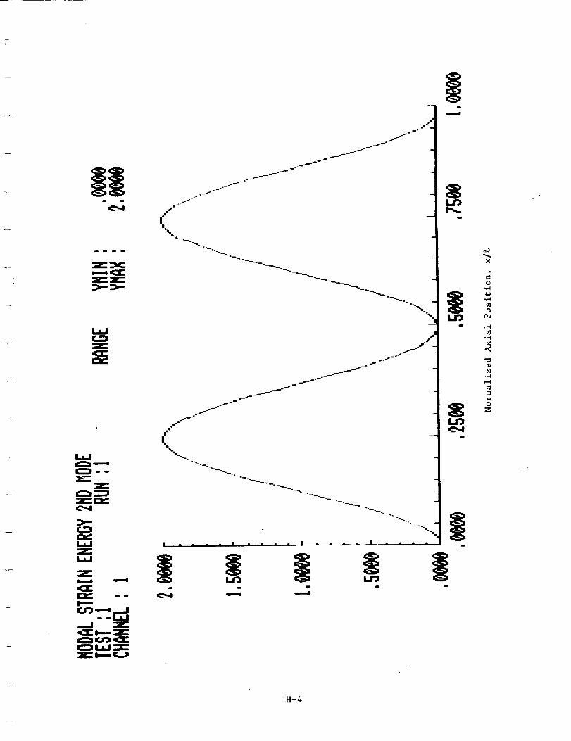
Z_
T- 'm'-
I.LI
V,III
ld
ILlZI.I,J
Z
. . I_L-IIr-,.I
_1 II::Z:::ll::: o.-- r_,Ji
m|_m""
m,",..
i
._os _
.,,me _°
_--.o__
----.,.
°°o_-
<
m
p,,..,.i
l.ml:mi
x
O
,.,.4
..,-I
0
..-.¢
N
,--¢
£H
Q
Z
1-I-4

o

o
o

mm Jl am I
LJ'J
|
Z-Z-7

||
H-8

r

||
_ga_
o
o
oZ
co
|
I-I-10
|

Z=)qC
Z
E
WZW
P_- ,,41
_j--j .,-q ,_j. ,.LLJ
•-J Z'_Z
H-If
|i
a
8m
|
X
O
,-4
"I,,4
N
@Z

_mmm
o g
|
H-12
|

|
H-13

|
_ o m
Z
-°
H-14

NASA SCIENTIFtC AND TECP.NtCAL _CUMENT AVAILABILITY AUTHORIZATION (DAA)
To be initiated by the responsible NASA Project Officer. Technical Monitor. or other appropriate I (Facility Use Only)
NASA offictal for all presentations reports papers and proceedings that contain scientific _ Or gtnal I
and technical information. Explanations a_e on the' back of this form and are prese-*_'4 i,,_ U-- Modified II Centre' No.
greater detail in NHB 2200.2, "NASA Scientific and Technical Information Handbook." I Date
I. DOCt.,UMENT/pP_O,JECTIDF.NTIFICATION (Infoqne_o_ copta_ed on report do_cum!_l'ltatJ, on,LpegJ_ shpuld not b_ repeet,,ej:l exce.pt title, date and Conlracl number) SBIR
Title: yrovlalng Strucuura± FIOGUleS wlEn bel[-lnuegrlcy monlcorlngPhase II
Author(s);
Originating NASA Organlzatlon: NASA Resident Office-JPL
PerformlngOrganizatlontltdlfferent)Anco Engineers. Inc.Contract/GrsnUInteregency/Project Number(s) NAS7-961
Document Number(s) DocumentDate:1 / 6 / 8 6-- 7 / 6
(For presentations or externally published documents, enter appropriate information on the Intended publication such as name. place, and date of conference, periodical Or Journal title.
or book title and publisher:
These documents must be routed to NASA Headquarters, International Affairs Division for approval. (See Section VII))
II. AVAILABILITY CATEGORY
Checktheappropriate / IV-- ,...... i:Security Classification: [] Secret [] Secret RD [] Confidential [] Contidential RD [] Unclassified
Export Control|ed Document - Documents marked in this block must be routed to NASA Headquarters International Affairs Division for approval. Z_-_ ," "/ ;- /*` "/' " "('
[] ITAR C] EAR /NASA Restricted Distribution Document - _-_'
[] FEDD [] Limited Distribution [_Spsctal Conditions-See Section III
Document disclosing an invention p ,'_,_"_,,'_
D Documents marked In this block must be withheld from release until all( month= have elapsed alter submission of this form, unless a different releise / _ "_L__) _,_
date Is established by the appropriate counsel. (See Section IX). ¢J _"--J _ _-
Publicly Available Document • ,_r
[] Publicly available documents must be unclassified and may not be export-controlled or restricted distribution documents. _ ,_F
[_ Copyrighted [] Not copyrighted I ,/"
IlL SPECIAL CONDITIONS " ' ' % ,_
Check one or more of the applicable boxes tn each of (a) and (b) as the basis for special restricted distribution if the "Special Conditions" box und_ASA j_"
Restricted Distribution Document in Section II is checked. Guidelines are provided on reverse side of form. '_
a. T_For%Cigm_tv_Orntrn, ie_: niormatio n [] Commercial product test or evaluation results [] Prel,minary information _ Information s_ special contract provision
OOther-Spec,__ SBIR-P_prlq_ary for twob. Checkoneof,_folio.tng,m._tionsa_e_ropriato: yeaj_a_ter _ept ance
[] U.S. Government agencies end US. Government agency contractors only [] NASA contractors and U.S. Government agen_ JK3 U.S GovernrR_agencles only
rJNASA_.,rso,,,.,ter,dNASAco,,trec,orson,y r_NAS._rs.... ,o,,,y []A_e_'ItY'I_°f._P,_h°_"_/ad: 9/26/88 _--
IV. BLANKET RELEASE (OPTIONAL)
All documents Issued under the following .£,ontract/granUproject number
The blanket release authorization granted is:Date
(_ Rescinded - Future documents must have individual availability authorizations.
PROJECTOFFICER/TECHNICALMONITORGordon S. Chapman SJT
"F/pad Name of Project Officer/Tschnical Monitor Olflce Code
may be processed as checked in Sectons II and IlL
[_ Modified - Limitations for all documenls processed in the STI system under the blanket
release should be changed to conform to blocks as checked In Section II.
VI. PROGRAM OFFICE REVIEW [] Approved [] Not Approved
Typed Name of Program Office Representative Program Office and Code Signature Date
VII, INTERNATIONAL AFFAIRS DIVISION REVIEW
[] Open. domestic conference presentation approved.
[] Foreign publication/presentation approved.
[] Export controlled limitation is approved.
[] Export controlled limitation is not applicable.
The Io/iowing Export controlled limitation (ITAR/EAR) is assigned to this document:
International Affairs Div, Representative Title Date
VIII. EXPIRATION OF REVIEW TIME
The document is being released in accordance with the availability category and limitation checked In Section II since no objection wee received from the Program
Office within 20 days of submission, as specified by NHB 2200.2, and approval by the International Affairs Division Is not required,
Name & Title Office Code
Note: This release procedure cannot be used with documents designated as Export Controlled Documents. conference presentations or foreign publications.
Date __
IX. DOCUMENTS DISCLOSING AN INVENTION
a. This document may be releas_l onDate
The document was peocessed on ,.
Date
Installation Patent or Intellectual Properly Counsel
In accordance with Sections If and Ill as applicable.
Dale
NASA STI Facility Date ____
ISPOSITION
,ted forms should be forwarded to the NASA Scientific end Technical
lion Fl|clllty, P.O. Box $757, B.W.I. Airport, Maryland 21240, with
'eck box):
ted or rewoducible copy of document enclosed
• act or Report Documentalion Pegs enclosed. The issuing or sponsoring NASA installation should provide a copy of the document, when complete.
' NASA Sclentilic and Technical Informalioff Facility at the above listed address.
.eport
88
r'427 REV OCTR6