Naıve Learning in Social Networks and theWisdom of Crowds∗

Benjamin Golub†and Matthew O. Jackson‡

Forthcoming: American Economic Journal Microeconomics

∗We thank Francis Bloch, Antoni Calvo-Armengol, Drew Fudenberg, Tim Roughgarden, Jonathan We-instein, the editor, and two anonymous referees for helpful comments and suggestions. Financial supportunder NSF grant SES-0647867 is gratefully acknowledged.

†Graduate School of Business, Stanford University, Stanford, CA, 94305-5015.http://www.stanfore.edu/∼bgolub e-mail: bgolub@stanford.edu

‡Department of Economics, Stanford University, Stanford, CA, 94305-6072.http://www.stanford.edu/∼jacksonm e-mail: jacksonm@stanford.edu

1

Naıve Learning in Social Networksand the Wisdom of Crowds

By Benjamin Golub and Matthew O. Jackson∗

January 14, 2007Revised: April 17, 2009

We study learning and influence in a setting where agents receive inde-pendent noisy signals about the true value of a variable of interest andthen communicate according to an arbitrary social network. The agentsnaıvely update their beliefs over time in a decentralized way by repeat-edly taking weighted averages of their neighbors’ opinions. We identifyconditions determining whether the beliefs of all agents in large societiesconverge to the true value of the variable, despite their naıve updating.We show that such convergence to truth obtains if and only if the in-fluence of the most influential agent in the society is vanishing as thesociety grows. We identify obstructions which can prevent this, includ-ing the existence of prominent groups which receive a disproportionateshare of attention. By ruling out such obstructions, we provide struc-tural conditions on the social network that are sufficient for convergenceto the truth. Finally, we discuss the speed of convergence and note thatwhether or not the society converges to truth is unrelated to how quicklya society’s agents reach a consensus.JEL: D85, D83, A14, L14, Z13.Keywords: social networks, learning, diffusion, conformism, bounded ra-tionality.

Social networks are primary conduits of information, opinions, and behaviors. Theycarry news about products, jobs, and various social programs; influence decisions tobecome educated, to smoke, and to commit crimes; and drive political opinions and atti-tudes toward other groups. In view of this, it is important to understand how beliefs andbehaviors evolve over time, how this depends on the network structure, and whether ornot the resulting outcomes are efficient. In this paper we examine one aspect of this broadtheme: for which social network structures will a society of agents who communicate andupdate naıvely come to aggregate decentralized information completely and correctly?

Given the complex forms that social networks often take, it can be difficult for theagents involved (or even for a modeler with full knowledge of the network) to updatebeliefs properly. For example, Syngjoo Choi, Douglas Gale and Shachar Kariv (2005,2008) find that although subjects in simple three-person networks update fairly well

∗ Golub: Graduate School of Business, Stanford University, Stanford, CA, 94305-5015,bgolub@stanford.edu. Jackson: Department of Economics, Stanford University, Stanford, CA, 94305-6072, and the Santa Fe Institute, Santa Fe, NM 87501. We thank Francis Bloch, Antoni Calvo-Armengol,Drew Fudenberg, Tim Roughgarden, Jonathan Weinstein, and two anonymous referees for helpful com-

ments and suggestions. Financial support under NSF grant SES-0647867 and the Thomas C. HaysFellowship at Caltech is gratefully acknowledged.

1

2

in some circumstances, they do not do so well in evaluating repeated observations andjudging indirect information whose origin is uncertain. Given that social communicationoften involves repeated transfers of information among large numbers of individuals incomplex networks, fully rational learning becomes infeasible. Nonetheless, it is possiblethat agents using fairly simple updating rules will arrive at outcomes like those achievedthrough fully rational learning. We identify social networks for which naıve individualsconverge to fully rational beliefs despite using simple and decentralized updating rulesand we also identify social networks for which beliefs fail to converge to the rational limitunder the same updating.

We base our study on an important model of network influence largely due to MorrisH. DeGroot (1974). The social structure of a society is described by a weighted andpossibly directed network. Agents have beliefs about some common question of interest –for instance, the probability of some event. At each date, agents communicate with theirneighbors in the social network and update their beliefs. The updating process is simple:an agent’s new belief is the (weighted) average of his or her neighbors’ beliefs from theprevious period. Over time, provided the network is strongly connected (so there is adirected path from any agent to any other) and satisfies a weak aperiodicity condition,beliefs converge to a consensus. This is easy to understand: at least one agent with thelowest belief must have a neighbor who has a higher belief, and similarly, some agentwith the highest belief has a neighbor with a lower belief, so distance between highestand lowest beliefs decays over time.

We focus on situations where there is some true state of nature that agents are tryingto learn and each agent’s initial belief is equal to the true state of nature plus someidiosyncratic zero-mean noise. An outside observer who could aggregate all of the decen-tralized initial beliefs could develop an estimate of the true state that would be arbitrarilyaccurate in a large society. Agents using the DeGroot rule will converge to a consensusestimate. Our question is: for which social networks will agents using the simple andnaıve updating process all converge to an accurate estimate of the true state?

The repeated updating model we use is simple, tractable, and captures some of thebasic aspects of social learning, so it is unsurprising that it has a long history. Its rootsgo back to sociological measures of centrality and prestige that were introduced by LeoKatz (1953) and further developed by Phillip B. Bonacich (1987). There are precursors,reincarnations, and cousins of the framework discussed by John R. P. French, Jr. (1956),Frank Harary (1959), Noah E. Friedkin and Eugene C. Johnsen (1997), and Peter M.DeMarzo, Dimitri Vayanos and Jeffrey Zwiebel (2003), among others. In the DeGrootversion of the model that we study, agents update their beliefs or attitudes in each periodsimply by taking weighted averages of their neighbors’ opinions from the previous period,possibly placing some weight on their own previous beliefs. The agents in this scenarioare boundedly rational, failing to adjust correctly for repetitions and dependencies ininformation that they hear multiple times.1 While this model captures the fact that

1For more discussion and background on the form of the updating, there are several sources. ForBayesian foundations under some normality assumptions, see DeGroot (2002, pp. 416–417). Behavioral

explanations are discussed in Friedkin and Johnsen (1997) and DeMarzo, Vayanos and Zwiebel (2003).

3

agents repeatedly communicate with each other and incorporate indirect information ina boundedly rational way, it is rigid in that agents do not adjust the weights they place onothers’ opinions over time. Nonetheless, it is a useful and tractable first approximationthat serves as a benchmark. In fact, the main results of the paper show that even thisrigid and naıve process can still lead agents to converge jointly to fully accurate beliefsin the limit as society grows large in a variety of social networks. Moreover, the limitingproperties of this process are useful not only for understanding belief evolution, but alsoas a basis for analyzing the influence or power of the different individuals in a network.2

Our contributions are outlined as follows, in the order in which they appear in thepaper.

Section I introduces the model, discusses the updating rule, and establishes some def-initions. Then, to lay the groundwork for our study of convergence to true beliefs, webriefly review issues of convergence itself in Section II. Specifically, for strongly connectednetworks, we state the necessary and sufficient condition for all agents’ beliefs to convergeas opposed to oscillating indefinitely; the condition is based on the well-known charac-terization of Markov chain convergence. When beliefs do converge, they converge to aconsensus. In Section A of the appendix we provide a full characterization of convergenceeven for networks that are not strongly connected, based on straightforward extensionsof known results from linear algebra.

When convergence obtains, the consensus belief is a weighted average of agents’ initialbeliefs and the weights provide a measure of social influence or importance. Those weightsare given by a principal eigenvector of the social network matrix. This is what makes theDeGroot model so tractable, and we take advantage of this known feature to trace howinfluential different agents are as a function of the structure of the social network. Thisleads us to the novel theoretical results of the paper. In Sections III and IV, we ask forwhich social networks will a large society of naıve DeGroot updaters converge to beliefssuch that all agents learn the true state of nature, assuming that they all start withindependent (but not necessarily identically distributed) noisy signals about the state.For example, if all agents listen to just one particular agent, then their beliefs converge,but they converge to that agent’s initial information, and thus the beliefs are not accurate,in the sense that they have a substantial probability of deviating substantially from thetruth. In contrast, if all agents place equal weight on all agents in their communication,then clearly they immediately converge to an average of all of the signals in the society,and then, by a law of large numbers, agents in large societies all hold beliefs close tothe true value of the variable. We call networked societies that converge to this accuratelimit “wise”. The question is what happens for large societies that are more complexthan those two extremes.

Our main results begin with a simple but complete characterization of wisdom in termsof influence weights in Section III: a society is wise if and only if the influence of the most

For additional results from other versions of the model, see Jackson (2008).2The model can also be applied to study a myopic best-response dynamic of a game in which agents

care about matching the behavior of those in their social network (possibly placing some weight onthemselves).

4

influential agent is vanishing as the society grows. Building on this characterization,we then focus on the relationship between social structure and wisdom in Section IV.First, in a setting where all ties are reciprocal and agents pay equal attention to alltheir neighbors, wisdom can fail if and only if there is an agent whose degree (numberof neighbors) is a nonvanishing fraction of the the total number of links in the network,no matter how large the network grows; thus, in this setting, disproportionate popularityis the sole obstacle to wisdom. Moving to more general results, we show that havinga bounded number of agents who are prominent (receiving a nonvanishing amount ofpossibly indirect attention from everyone in the network) causes learning to fail, sincetheir influence on the limiting beliefs is excessive. This result is a fairly direct elaborationof the characterization of wisdom given above, but it is stated in terms of the geometryof the network as opposed to the influence weights. Next, we provide examples of typesof network patterns that prevent a society from being wise. One is a lack of balance,where some groups get much more attention than they give out, and the other is alack of dispersion, where small groups do not pay sufficient attention to the rest of theworld. Based on these examples, we formulate structural conditions that are sufficientfor wisdom. The sufficient conditions formally capture the intuition that societies withbalance and dispersion in their communication structures will have accurate learning.

In Section V, we discuss some of what is known about the speed and dynamics of theupdating process studied here. Understanding the relationship between communicationstructures and the persistence of disagreement is independently interesting, and also shedslight on when steady-state analysis is relevant. We note that the speed of convergence isnot related to wisdom.

The proofs of all results in the sections just discussed appear in Section B of theappendix; some additional results, along with their proofs, appear in Sections A and Cof the appendix.

Our work relates to several lines of research other than the ones already discussed.There is a large theoretical literature on social learning, both fully and boundedly ratio-nal. Herding models (e.g., Abhijit V. Banerjee (1992), Sushil Bikhchandani, David Hir-shleifer and Ivo Welch (1992), Glenn Ellison and Drew Fudenberg (1993, 1995), Gale andKariv (2003), Bogachan Celen and Kariv (2004), and Banerjee and Fudenberg (2004))are prime examples, and there agents converge to holding the same belief or at leastthe same judgment as to an optimal action. These conclusions generally apply to ob-servational learning, where agents are observing choices and/or payoffs over time andupdating accordingly.3 In such models, the structure determining which agents observewhich others when making decisions is typically constrained, and the learning results donot depend sensitively on the precise structure of the social network. Our results arequite different from these. In contrast to the observational learning models, convergenceand the efficiency of learning in our model depend critically on the details of the networkarchitecture and on the influences of various agents.

The work of Venkatesh Bala and Sanjeev Goyal (1998) is closer to the spirit of our

3For a general version of the observational learning approach, see Dinah Rosenberg, Eilon Solan andNicolas Vieille (2006).

5

work, as they allow for richer network structures. Their approach is different from oursin that they examine observational learning where agents take repeated actions and canobserve each other’s payoffs. There, consensus within connected components generallyobtains because all agents can observe whether their neighbors are earning payoffs differ-ent from their own.4 They also examine the question of whether agents might convergeto taking the wrong actions, which is a sort of wisdom question, and the answer dependson whether some agents are too influential – which has some similar intuition to theprominence results that we find in the DeGroot model. Bala and Goyal also providesufficient conditions for convergence to the correct action; roughly speaking, these re-quire (i) some agent to be arbitrarily confident in each action, so that each action getschosen enough to reveal its value; and (ii) the existence of paths of agents observing eachsuch agent, so that the information diffuses. While the questions we ask are similar,the analysis and conclusions are quite different in two important ways: first, the purecommunication which we study is different from observational learning, and that changesthe sorts of conditions that are needed for wisdom; second, the DeGroot model allowsfor precise calculations of the influence of every agent in any network, which is not seenin the observational learning literature. The second point is obvious, so let us explainthe first aspect of the difference, which is especially useful to discuss since it highlightsfundamental differences between issues of learning through repeated observation and ac-tions, and updating via repeated communication. In the observational learning setting,if some agent is sufficiently stubborn in pursuing a given action, then through repeatedobservation of that action’s payoffs, the agent’s neighbors learn that action’s value if it issuperior; then that leads them to take the action, and then their neighbors learn, and soforth. Thus to be arbitrarily sure of converging to the best action, all that is needed is foreach action to have a player who has a prior that places sufficiently high weight on thataction so that its payoff will be sufficiently accurately assessed; and if it turns out to bethe highest payoff action it will eventually diffuse throughout the component regardlessof network structure. In contrast, in the updating setting of the DeGroot model, everyagent starts with just one noisy signal and the question is how that decentralized infor-mation is aggregated through repeated communication. Generally, we do not require anyagent to have an arbitrarily accurate signal, nor would this circumstance be sufficient forwisdom except for some very specific network structures. In this repeated communicationsetting, signals can quickly become mixed with other signals, and the network structure iscritical to determining what the ultimate mixing of signals is. So, the models, questions,basic structure, and conclusions are quite different between the two settings even thoughthere are some superficial similarities.

Closer in terms of the formulation, but less so in terms of the questions asked, is thestudy by DeMarzo, Vayanos and Zwiebel (2003), which focuses mainly on a network-based explanation for the “unidimensionality” of political opinions. Nevertheless, theydo present some results on the correctness of learning. Our results on sufficient conditionsfor wisdom may be compared with their Theorem 2, where they conclude that consensus

4Bala and Goyal (2001) show that heterogeneity in preferences in the society can cause similarindividuals to converge to different actions if they are not connected.

6

beliefs (for a fixed population of n agents) optimally aggregate information if and onlyif a knife-edge restriction on the weights holds. Our results show that under much lessrestrictive conditions, aggregation can be asymptotically accurate even if it is not optimalin finite societies. More generally, our conclusions differ from a long line of previous workwhich suggests that sufficient conditions for naıve learning are hopelessly strong.5 Weshow that beliefs can be correct in the large-society limit for a fairly broad collection ofnetworks.

The most recent work on this subject of which we are aware is a paper (following thefirst version of this paper) by Daron Acemoglu, Munther Dahleh, Ilan Lobel, and AsumanOzdaglar (2008), which is in the rational observational learning paradigm but relates toour work in terms of the questions asked and the spirit of the main results; the paper bothcomplements and contrasts with ours. In that model, each agent makes a decision oncein a predetermined order and observes previous agents’ decisions according to a randomprocess whose distribution is common knowledge. The main result of the paper is that ifagents have priors which allow signals to be arbitrarily informative, then the absence ofagents who are excessively influential is enough to guarantee convergence to the correctaction. The definition of excessive influence is demanding: to be excessively influential,a group must be finite and must provide all the information to an infinite group of otheragents. Conversely, an excessively influential group in this sense destroys social learning.The structure of the model is quite different from ours: the agents of Acemoglu, Dahleh,Lobel and Ozdaglar (2008) take one action as opposed to updating constantly, and thelearning there is observational. Nevertheless, these results are interesting to compare withour main theorems since actions are taken only once and so the model is somewhat closerto the setting we study than the learning from repeated observations discussed above. Aswe mentioned, prominent groups can also destroy learning in our model and ruling themout is a first step in guaranteeing wisdom. However, our notion of prominence is differentfrom and, intuitively speaking, not as strong as the notion of excessive influence: to beprominent in our setting a group must only get some attention from everyone, as opposedto providing all the information to a very large group. Thus, our agents are more easilymisled, and the errors that can happen depend more sensitively on the details of thenetwork structure. This is natural: since they are more naıve, social structure mattersmore in determining the outcome. We view the approaches of Acemoglu et al. (2008) andour work as being quite complementary in the sense that some of these differences aredriven by differences in agents’ rationality. However, there are also more basic differencesbetween the models in terms of what information represents, as well as the repetition,timing, and patterns of communication.

In addition, there are literatures in physics and computer science on the DeGroot modeland variations on it.6 There, the focus has generally been on consensus rather than onwisdom. In sociology, since the work of Katz (1953), French (1956), and Bonacich (1987),eigenvector-like notions of centrality and prestige have been analyzed.7 As some such

5See Joel Sobel (2000) for a survey.6See Section 8.3 of Jackson (2008) for an overview and more references.7See also Stanley Wasserman and Katherine Faust (1994), Phillip P. Bonacich and Paulette Lloyd

7

models are based on convergence of iterated influence relationships, our results provideinsight into the structure of the influence vectors in those models, especially in the large-society limit. Finally, there is an enormous empirical literature about the influence ofsocial acquaintances on behavior and outcomes that we will not attempt to survey here,8

but simply point out that our model provides testable predictions about the relationshipsbetween social structure and social learning.

I. The DeGroot Model

A. Agents and Interaction

A finite set N = {1, 2, . . . , n} of agents or nodes interact according to a social network.The interaction patterns are captured through an n × n nonnegative matrix T, whereTij > 0 indicates that i pays attention to j. The matrix T may be asymmetric, andthe interactions can be one-sided, so that Tij > 0 while Tji = 0. We refer to T asthe interaction matrix. This matrix is stochastic, so that its entries across each row arenormalized to sum to 1.

B. Updating

Agents update beliefs by repeatedly taking weighted averages of their neighbors’ beliefswith Tij being the weight or trust that agent i places on the current belief of agent jin forming his or her belief for the next period. In particular, each agent has a beliefp(t)i ∈ R at time t ∈ {0, 1, 2, . . .}. For convenience, we take p(t)

i to lie in [0,1], althoughit could lie in a multi-dimensional Euclidean space without affecting the results below.The vector of beliefs at time t is written p(t). The updating rule is:

p(t) = Tp(t−1)

and so

(1) p(t) = Ttp(0).

The evolution of beliefs can be motivated by the following Bayesian setup discussedby DeMarzo, Vayanos and Zwiebel (2003). At time t = 0 each agent receives a noisysignal p(0)

i = µ + ei where ei ∈ R is a noise term with expectation zero and µ is somestate of nature. Agent i hears the opinions of the agents with whom he interacts, andassigns precision πij to agent j. These subjective estimates may, but need not, coincidewith the true precisions of their signals. If agent i does not listen to agent j, then agenti gives j precision πij = 0. In the case where the signals are normal, Bayesian updatingfrom independent signals at t = 1 entails the rule (1) with Tij = πij/

∑nk=1 πik. As

(2001) and Jackson (2008) for more recent elaborations.8The Handbook of Social Economics (Jess Benhabib, Alberto Bisin and Matthew O. Jackson

(forthcoming)) provides overviews of various aspects of this.

8

agents may only be able to communicate directly with a subset of agents due to someexogenous constraints or costs, they will generally wish to continue to communicate andupdate based on their neighbors’ evolving beliefs, since that allows them to incorporateindirect information. The key behavioral assumption is that the agents continue usingthe same updating rule throughout the evolution. That is, they do not account for thepossible repetition of information and for the “cross-contamination” of their neighbors’signals. This bounded rationality arising from persuasion bias is discussed at length byDeMarzo, Vayanos and Zwiebel (2003), and so we do not reiterate that discussion here.

It is important to note that other applications also have the same form as that analyzedhere. What we refer to as “beliefs” could also be some behavior that people adjust inresponse to their neighbors’ behaviors, either through some desire to match behaviorsor through other social pressures favoring conformity. As another example, Google’s“PageRank” system is based on a measure related to the influence vectors derived below,where the T matrix is the normalized link matrix.9 Other citation and influence measuresalso have similar eigenvector foundations (e.g., see Ignacio Palacios-Huerta and OscarVolij (2004)). Finally, we also see iterated interaction matrices in studies of recursiveutility (e.g., Brian W. Rogers (2006)) and in strategic games played by agents on networkswhere influence measures turn out to be important (e.g., Coralio Ballester, Antoni Calvo-Armengol and Yves Zenou (2006)). In such applications understanding the properties ofTt and related matrices is critical.

C. Walks, Paths and Cycles

The following are standard graph-theoretic definitions applied to the directed graph ofconnections induced by the interaction matrix T.

A walk in T is a sequence of nodes i1, i2, . . . , iK , not necessarily distinct, such thatTikik+1 > 0 for each k ∈ {1, . . . ,K − 1}. The length of the walk is defined to be K − 1.A path in T is a walk consisting of distinct nodes.

A cycle is a walk i1, i2, . . . , iK such that i1 = iK . The length of a cycle with K (notnecessarily distinct) entries is defined to be K − 1. A cycle is simple if the only nodeappearing twice in the sequence is the starting (and ending) node.

The matrix T is strongly connected if there is path in T from any node to any othernode. Similarly, we say that B ⊂ N is strongly connected if T restricted to B is stronglyconnected. This is true if and only if the nodes in B all lie on a cycle that involves onlynodes in B. If T is undirected in the sense that Tij > 0 if and only if Tji > 0, then wesimply say the matrix is connected.

II. Convergence of Beliefs Under Naıve Updating

We begin with the question of when the beliefs of all agents in a network converge towell-defined limits as opposed to oscillating forever. Without such convergence, it is clear

9So Tij = 1/`i if page i has a link to page j, where `i is the number of links that page i has to otherpages. From this basic form T is perturbed for technical reasons; see Amy N. Langville and Carl D.Meyer (2006) for details.

9

that wisdom could not be obtained.

DEFINITION 1: A matrix T is convergent if limt→∞Ttp exists for all vectors p ∈[0, 1]n.

This definition of convergence requires that beliefs converge for all initial vectors ofbeliefs. Clearly, any network will have convergence for some initial vectors, since if westart all agents with the same beliefs then no nontrivial updating will ever occur. It turnsout that if convergence fails for some initial vector, then there will be cycles or oscillationsin the updating of beliefs and convergence will fail for whole classes of initial vectors.

A condition ensuring convergence in strongly connected stochastic matrices is aperiod-icity.

DEFINITION 2: The matrix T is aperiodic if the greatest common divisor of the lengthsof its simple cycles is 1.

A. Examples

The following very simple and standard example illustrates of a failure of aperiodicity.

EXAMPLE 1:

T =(

0 11 0

).

Clearly,

Tt =

{T if t is odd

I if t is even.

In particular, if p1(0) 6= p2(0), then the belief vector never reaches a steady state and thetwo agents keep switching beliefs.

Here, each agent ignores his own current belief in updating. Requiring at least oneagent to weight his current belief positively ensures convergence; this is a special case ofProposition 1 below. However, it is not necessary to have Tii > 0 for even a single i inorder to ensure convergence.

EXAMPLE 2: Consider

T =

0 1/2 1/21 0 00 1 0

.

Here,

Tt →

2/5 2/5 1/52/5 2/5 1/52/5 2/5 1/5

.

Even though T has only 0 along its diagonal, it is aperiodic and converges. If we changethe matrix to

T =

0 1/2 1/21 0 01 0 0

,

10

then T is periodic as all of its cycles are of even lengths and T is no longer convergent.

B. A Characterization of Convergence and Limiting Beliefs

It well-known that aperiodicity is necessary and sufficient for convergence in the casewhere T is strongly connected (John G. Kemeny and J. Laurie Snell (1960)). We sum-marize this in the following statement.

PROPOSITION 1: If T is a strongly connected matrix, the following are equivalent:

(i) T is convergent.

(ii) T is aperiodic.

(iii) There is a unique left eigenvector s of T corresponding to eigenvalue 1 whose entriessum to 1 such that, for every p ∈ [0, 1]n,(

limt→∞

Ttp)i

= sp

for every i.

In addition to characterizing convergence, this fact also establishes what beliefs con-verge to when they do converge. The limiting beliefs are all equal to a weighted averageof initial beliefs, with agent i’s weight being si. We refer to si as the influence weight orsimply the influence of agent i.

To see why there is an eigenvector involved, let us suppose that we would like to finda vector s = (s1, . . . , sn) ∈ [0, 1]n which would measure how much each agent influencesthe limiting belief. In particular, let us look for a nonnegative vector, normalized so thatits entries sum to 1, such that for any vector of initial beliefs p ∈ [0, 1]n, we have(

limt→∞

Ttp)j

=∑i

sipi(0).

Noting that limt→∞Ttp = limt→∞Tt (Tp), it must be that

sp = sTp,

for every p ∈ [0, 1]n. This implies that s = sT, and so s is simply a unit (left-hand orrow) eigenvector of T, provided that such an s can be found.

The eigenvector property, of course, is just saying that sj =∑i∈N Tijsi for all j, so

that the influence of i is a weighted sum of the influences of various agents j who payattention to i, with the weight of sj being the trust of j for i. This is a very naturalproperty for a measure of influence to have and entails that influential people are thosewho are trusted by other influential people.

As mentioned in the introduction, the result can be generalized to situations withoutstrong connectedness, which are relevant for many applications. This is discussed in

11

Section A of the appendix. Much of the structure discussed above remains in that case,with some modifications, but some aspects of the characterization, such as the equalityof everyone’s limiting beliefs, do not hold in general settings.

C. Undirected Networks with Equal Weights

A particularly tractable special case of the model arises when T is derived from havingeach agent equally split attention among his or her neighbors in an undirected network.Suppose that we start with a symmetric, connected adjacency matrix G of an undirectednetwork, where Gij = 1 indicates that i and j have an undirected link between themand Gij = 0 otherwise. Let di(G) =

∑nj=1Gij be the degree, or number of neighbors, of

agent i. Then, if we define T(G) by Tij = Gij/di(G), we obtain a stochastic matrix. Theinterpretation is that G gives a social network of undirected connections, and everyoneputs equal weight on all his neighbors in that network.10 It is impossible, in this setting,for i to pay attention to j and not vice versa, and it is not possible for someone to paydifferent amounts of attention to different sources that he or she listens to. Thus, thissetting places some real restrictions on the structure of the interaction matrix, but, inreturn, yields a very intuitive characterization of influence weights. Indeed, as pointedout in DeMarzo, Vayanos and Zwiebel (2003), the vector s has a simple structure:

si =di(G)∑ni=1 di(G)

,

as can be verified by a direct calculation, using Proposition 1(iii). Thus, in this specialcase, influence is directly proportional to degree.

III. The Wisdom of Crowds: Definition and Characterization

With the preliminaries out of the way, we now turn to the central question of the paper:under what circumstances does the decentralized DeGroot process of communicationcorrectly aggregate the diverse information initially held by the different agents? Inparticular, we are interested in large societies. The large-society limit is relevant inmany applications of the theory of social learning. Moreover, a large number of agents isnecessary for there to be enough diversity of opinion for a society, even in the best case,to be able to wash out idiosyncratic errors and discover the truth.

To capture the idea of a “large” society, we examine sequences of networks where we letthe number of agents n grow and work with limiting statements. In discussing wisdom,we are taking a double limit. First, for any fixed network, we ask what its beliefs convergeto in the long run. Next, we study limits of these long-run beliefs as the networks grow;the second limit is taken across a sequence of networks.

The sequence of networks is captured by a sequence of n-by-n interaction matrices: wesay that a society is a sequence (T(n))∞n=1 indexed by n, the number of agents in each

10In Markov chain language, T(G) corresponds to a symmetric random walk on an undirected graph,and the Markov chain is reversible (Persi Diaconis and Daniel Stroock (1991)).

12

network. We will denote the (i, j) entry of interaction matrix n by Tij(n), and, moregenerally, all scalars, vectors, and matrices associated to network n will be indicated byan argument n in parentheses.

Throughout this section, we maintain the assumption that each network is convergentfor each n; it does not make sense to talk about wisdom if the networks do not even haveconvergent beliefs, and so convergence is an a priori necessary condition for wisdom.11

Let us now specify the underlying probability space and give a formal definition of a wisesociety.

A. Defining Wisdom

There is a true state of nature µ ∈ [0, 1].12 We do not need to specify anything regardingthe distribution from which this true state is drawn; we treat the truth as fixed. If it isactually the realization of some random process, then all of the analysis is conditional onits realization.

At time t = 0, agent i in network n sees a signal p(0)i (n) that lies in a bounded set,

normalized without loss of generality to be [0, 1]. The signal is distributed with mean µ

and a variance of at least σ2 > 0, and the signals p(0)1 (n), . . . , p(0)

n (n) are independent foreach n. No further assumptions are made about the joint distribution of the variablesp(0)i (n) as n and i range over their possible values. The common lower bound on variance

ensures that convergence to truth is not occurring simply because there are arbitrarilywell informed agents in the society.13

Let s(n) be the influence vector corresponding to T(n), as defined in Proposition 1(or, more generally, Theorem 3). We write the belief of agent i in network n at time t asp(t)i (n).For any given n and realization of p(0)(n), the belief of each agent i in network n

approaches a limit which we denote by p(∞)i (n); the limits are characterized in Proposition

1 (or, more generally, Theorem 3). Each of these limiting beliefs is a random variablewhich depends on the initial signals. We say the sequence of networks is wise when thelimiting beliefs converge jointly in probability to the true state µ as n→∞.

DEFINITION 3: The sequence (T(n))∞n=1 is wise if,

plimn→∞

maxi≤n|p(∞)i (n)− µ| = 0.

While this definition is given with a specific distribution of signals in the background,it follows from Proposition 2 below that a sequence of networks will be wise for allsuch distributions or for none. Thus, the specifics of the distribution are irrelevant for

11We do not, however, require strong connectedness. All the results go through for general convergentnetworks; thus, some of the proofs use results in Section A of the appendix.

12This is easily extended to allow the true state to lie in any finite-dimensional Euclidean space, as

long as the signals that agents observe have a bounded support.13The lower bound on variance is only needed for one part of one result, which is the “only if” statement

in Lemma 1. Otherwise, one can dispose of this assumption.

13

determining whether a society is wise, provided the signals are independent, have meanµ, and have variances bounded away from 0. If these conditions are satisfied, the networkstructure alone determines wisdom.

B. Wisdom in Terms of Influence: A Law of Large Numbers

To investigate the question of which societies are wise, we first state a simple law oflarge numbers that is helpful in our setting, as we are working with weighted averagesof potentially non-identically distributed random variables. The following result will beused to completely characterize wisdom in terms of influence weights.

Without loss of generality, label the agents so that si(n) ≥ si+1(n) ≥ 0 for each i andn; that is, the agents are arranged by influence in decreasing order.

LEMMA 1: [A Law of Large Numbers] If (s(n))∞n=1 is any sequence of influence vectors,then

plimn→∞

s(n)p(0)(n) = µ

if and only if s1(n)→ 0.14

Thus, in strongly connected networks, the limiting belief of all agents,

p(∞)(n) =∑i≤n

si(n)p(0)i (n),

will converge to the truth as n→∞ if and only if the most important agent’s influencetends to 0 (recall that we labeled agents so that s1(n) is maximal among the si(n)). Withslightly more careful analysis, it can be shown that the same result holds whether or notthe networks are strongly connected, which is the content of the following proposition.

PROPOSITION 2: If (T(n))∞n=1 is a sequence of convergent stochastic matrices, thenit is wise if and only if the associated influence vectors are such that s1(n)→ 0.

This result is natural in view of the examples in Section IV.C below, which show that asociety can be led astray if the leader has too much influence. Indeed, the proofs of bothresults follow a very simple intuition: for the idiosyncratic errors to wash out and for thelimiting beliefs – which are weighted averages of initial beliefs – to converge to the truth,nobody’s idiosyncratic error should be getting positive weight in the large-society limit.

IV. Wisdom in Terms of Social Structure

The characterization in Section III is still abstract in that it applies to influence vectorsand not directly to the structure of the social network. It is interesting to see how wisdom

14Since∑

i≤n si(n)p(0)i (n) is bounded due to our assumption that p

(0)i (n) ∈ [0, 1] for each n and i,

the statement plimn→∞ s(n)p(0)(n) = µ is equivalent to having plimn→∞(|s(n)p(0)(n)− µ|r

)= 0 for

all r > 0.

14

is determined by the geometry of the network. Which structures prevent wisdom, andwhich ones ensure it? That is the focus of this section.

We begin with a simple characterization in the special case of undirected networks withequal weights discussed in Section II.C. After that, we state a general necessary conditionfor wisdom – the absence of prominent groups that receive attention from everyone insociety. However, simple examples show that when wisdom fails, it is not always possibleto identify an obvious prominent group. Ensuring wisdom is thus fairly subtle. Somesufficient conditions are given in the last subsection.

A. Wisdom in Undirected Networks with Equal Weights

A particularly simple characterization is obtained in the setting of Section II.C, whereagents weight their neighbors equally and communication is reciprocal. It is stated in thefollowing corollary of Proposition 2.

COROLLARY 1: Let (G(n))∞n=1 be a sequence of symmetric, connected adjacency ma-trices. The sequence (T (G(n)))∞n=1 is wise if and only if

max1≤i≤n

di(G(n))∑ni=1 di(G(n))

n−→ 0.

That is, a necessary and sufficient condition for wisdom in this setting is that themaximum degree becomes vanishingly small relative to the sum of degrees. In otherwords, disproportionate popularity of some agent is the only obstacle to wisdom.

While this characterization is very intuitive, it also depends on the special structure ofreciprocal attention and equal weights, as the examples in Section IV.C show.

B. Prominent Families as an Obstacle to Wisdom

We now discuss a general obstacle to wisdom in arbitrary networks: namely, the exis-tence of prominent groups which receive a disproportionate share of attention and leadsociety astray. This is reminiscent of the discussion in Bala and Goyal (1998) of whatcan go wrong when there is a commonly observed “royal family” under a different modelof observational learning. However, as noted in the introduction, the way in which thisworks and the implications for wisdom are quite different.15

15The similarity is that in both observational learning and in the repeated updating discussed here,having all agents concentrate their attention on a few agents can lead to societal errors if those few are in

error. The difference is in the way that this is avoided. In the observational learning setting, the sufficientcondition for complete learning of Bala and Goyal (1998) is for each action to be associated with some

very optimistic agent, and then to have every other agent have a path to every action’s correspondingoptimistic agent. Thus, the payoff to every action will be correctly figured out by its optimistic agent,and then society will eventually see which is the best of those actions. The only property of the networkthat is needed for this conclusion is connectedness. In our context, the analogue of this condition would

be to have some agent who observes the true state of nature with very high accuracy and then does notweight anyone else’s opinion. However, in keeping with our theme of starting with noisy information,

we are instead interested in when the network structure correctly aggregates many noisy signals, none ofwhich is accurate or persistent. Thus, our results do depend critically on network structure.

15

B C

TC,B

TB,C

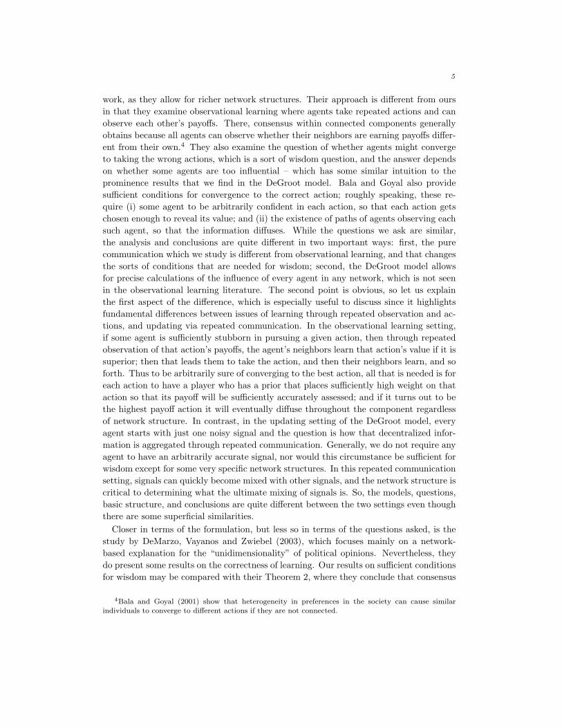
To introduce this concept, we need some definitions and notation. It is often useful toconsider the weight of groups on other groups. To this end, we define

TB,C =∑i∈Bj∈C

Tij

which is the weight that the group B places on the group C. The concept is illustratedin Figure B.

Returning to the setting of a fixed network of n agents for a moment, we begin bymaking a natural definition of what it means for a group to be observed by everyone.

DEFINITION 4: The group B is prominent in t steps relative to T if (Tt)i,B > 0 foreach i /∈ B.

Call πB(T; t) := mini/∈B(Tt)i,B the t-step prominence of B relative to T.

Thus, a group that is prominent in t steps is one such that each agent outside of it isinfluenced by at least someone in that group in t steps of updating. Note that the way inwhich the weight is distributed among the agents in the prominent group is left arbitrary,and some agents in the prominent group may be ignored altogether. If t = 1, theneveryone outside the prominent group is paying attention to somebody in the prominentgroup directly, i.e., not through someone else in several rounds of updating.

This definition is given relative to a single matrix T. While this is useful in derivingexplicit bounds on influence (see Section B of the appendix), we also define a notion ofprominence in the asymptotic setting. First, we define a family to be a sequence of groups(Bn) such that Bn ⊂ {1, . . . , n} for each n. A family should be thought of as a collectionof agents that may be changing and growing as we expand the society. In applications,the families could be agents of a certain type, but a priori there is no restriction on the

16

agents which are in the groups Bn. Now we can extend the notion of prominence tofamilies.

DEFINITION 5: The family (Bn) is uniformly prominent relative to (T(n))∞n=1 if thereexists a constant α > 0 such that for each n there is a t so that the group Bn is prominentin t steps relative to T(n) with πB(T(n); t) ≥ α.

For the family (Bn) to be uniformly prominent, we must have that for each n, the groupBn is prominent relative to T(n) in some number of steps without the prominence growingtoo small (hence the word “uniformly”). Note that at least one uniformly prominentfamily always exists, namely {1, . . . , n}.

We also define a notion of finiteness for families: a family is finite if it stops growingeventually.

DEFINITION 6: The family (Bn) is finite if there is a q such that supn |Bn| ≤ q.

With these definitions in hand, we can state a first necessary condition for wisdom interms of prominence: wisdom rules out finite, uniformly prominent families. This resultand the other facts in this section rely on bounds on various influences, as shown inSection B of the appendix.

PROPOSITION 3: If there is a finite, uniformly prominent family with respect to (T(n)),then the sequence is not wise.

To see the intuition behind this result, consider a special but illuminating example.Let (Bn) be a finite, uniformly prominent family so that, in the definition of uniformprominence, t = 1 for each n – that is, the family is always prominent in one step.Further, consider the strongly connected case, with agent i in network n getting weightsi(n). Normalize the true state of the world to be µ = 0, and for the purposes ofexposition suppose that everyone in Bn starts with belief 1, and that everyone outsidestarts with belief 0. Let α be a lower bound on the prominence of Bn. Then after oneround of updating, everyone outside Bn has belief at least α. So, for a large society, thevast majority of agents have beliefs that differ by at least α from the truth. The onlyway they could conceivably be led back to the truth is if, after one round of updating, atleast some agents in Bn have beliefs equal to 0 and can lead society back to the truth.Now we may forget what happened in the past and just view the current beliefs as newstarting beliefs. If the agents in Bn have enough influence to lead everyone back to 0forever when the other agents are α away from it, then they also have enough influenceto lead everyone away from 0 forever at the very start. So at best they can only lead thegroup part of the way back. Thus, we conclude that starting Bn with incorrect beliefsand everyone else with correct beliefs can lead the entire network to incorrect beliefs.

C. Other Obstructions to Wisdom: Examples

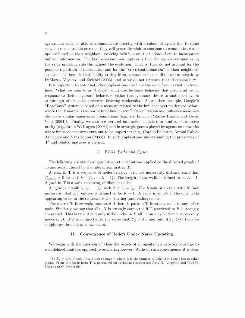
While prominence is a simple and important obstruction to wisdom, not all exampleswhere wisdom fails have a group that is prominent in a few steps. The following exampleboth illustrates Proposition 3 and demonstrates its limitations.

17

EXAMPLE 3: Consider the following network, defined for arbitrary n. Fix δ, ε ∈ (0, 1)and define, for each n ≥ 1, an n-by-n interaction matrix

T(n) :=

1− δ δ

n−1δ

n−1 · · · δn−1

1− ε ε 0 · · · 01− ε 0 ε · · · 0

......

.... . .

...1− ε 0 0 · · · ε

.

The network is shown in Figure 3 for n = 6 agents.

δ / (n – 1)

1 – ε

1– δ

ε

We find that

si(n) =

{1−ε

1−ε+δ if i = 1δ

(n−1)(1−ε+δ) if i > 1.

This network will not converge to the truth. Observe that in society n, the limitingbelief of each agent is s1(n)p(0)

1 (n) plus some other independent random variables thathave mean µ. As s1(n) is constant and independent of n, the variance of of the limitingbelief remains bounded away from 0 for all n. So beliefs will deviate from the truth bya substantial amount with positive probability. The intuition is simply that the leader’sinformation – even when it is far from the mean – is observed by everyone and weightedheavily enough that it biases the final belief, and the followers’ signals cannot do much tocorrect it. Indeed, Proposition 2 above establishes the lack of wisdom due to the nonvan-ishing influence of the central agent. If δ and ε are fixed constants, then the central agent(due to his position) is prominent in one step, making this an illustration of Proposition3.

However, note that even if we let 1 − ε approach 0 at any rate we like, so that peopleare not weighting the center very much, the center has nonvanishing influence as long as

18

1 − ε is of at least the order16 of δ. Thus, it is not simply the total weight on a givenindividual that matters, but the relative weights coming in and out of particular nodes(and groups of nodes). In particular, if the weight on the center decays (so that nobodyis prominent in one step), wisdom may still fail.

On the other hand, if 1 − ε becomes small relative to δ as society grows, then we canobtain wisdom despite the seemingly unbalanced social structure. This demonstrates thatthe result of Section IV.A is sensitive to the assumption that agents must place placeequal amounts of weight on each of their neighbors including themselves.

One thing that goes wrong in this example is that the central agent receives a highamount of trust relative to the amount given back to others, making him or her undulyinfluential. However, this is not the only obstruction to wisdom. There are examples inwhich the weight coming into any node is bounded relative to the weight going out, andthere is still an extremely influential agent who can keep society’s beliefs away from thetrue state. The next example shows how indirect weight can matter.

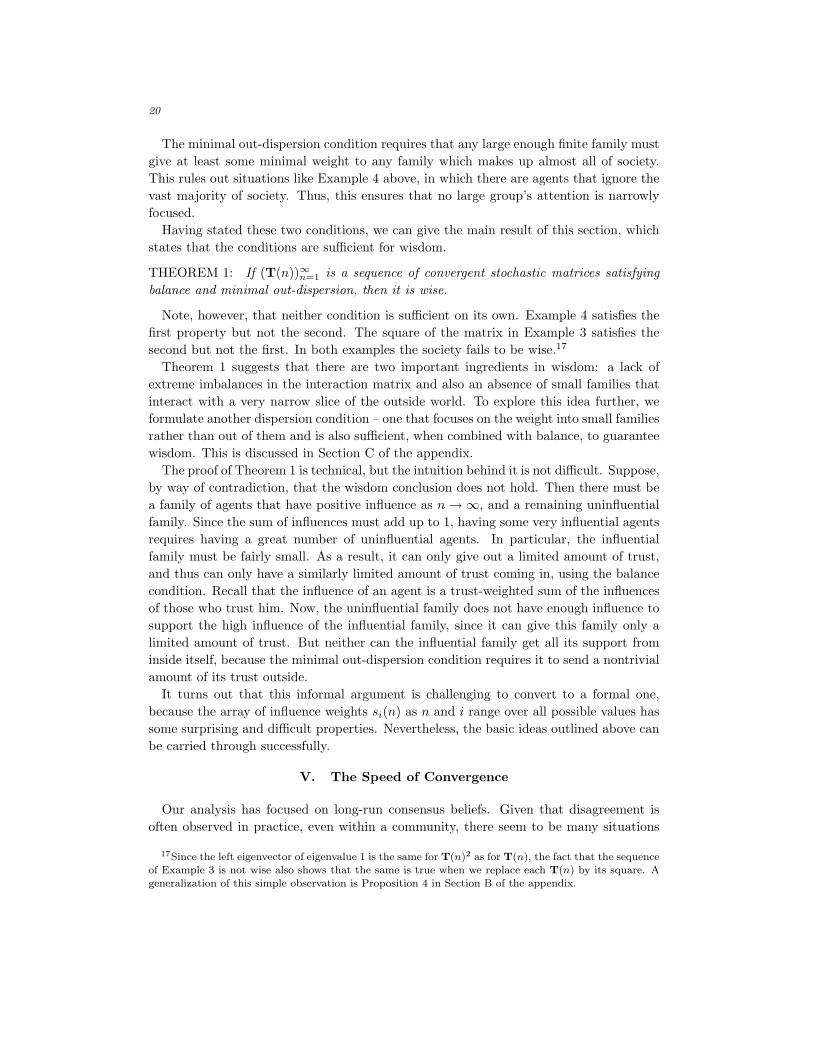
EXAMPLE 4: Fix δ ∈ (0, 1/2) and define, for each n ≥ 1, an n-by-n interaction matrixby

T11(n) = 1− δTi,i−1(n) = 1− δ if i ∈ {2, . . . , n}Ti,i+1(n) = δ if i ∈ {1, . . . , n− 1}Tnn(n) = δ

Tij(n) = 0 otherwise.

The network is shown in Figure 4.

δ

1– δ

δδ

1– δ

δ

1– δ

δ

1– δ

1– δ

. . .

It is simple to verify that

si(n) =(

δ

1− δ

)i−1

·1−

(δ

1−δ

)1−

(δ

1−δ

)n+1 .

In particular, limn→∞ s1(n) can be made as close to 1 as desired by choosing a small δ,and then Proposition 2 shows that wisdom does not obtain. The reason for the leader’sundue influence here is somewhat more subtle than in Example 3: it is not the weight

16Formally, suppose we have a sequence ε(n) and δ(n) with (1− ε(n))/δ(n) ≥ c > 0 for all n.

19

agent 1 directly receives, but indirect weight due to this agent’s privileged position in thenetwork. Thus, while agent 1 is not prominent in any number of steps less than n−1, theagent’s influence can exceed the sum of all other influences by a huge factor for small δ.This shows that it can be misleading to measure agents’ influence based on direct incomingweight or even indirect weight at a few levels; instead, the entire structure of the networkis relevant.

D. Ensuring Wisdom: Structural Sufficient Conditions

We now provide structural sufficient conditions for a society to be wise. The examplesof the previous subsection make it clear that wisdom is, in general, a subtle property.Thus, formulating the sufficient conditions requires defining some new concepts, whichcan be used to rule out obstructions to wisdom.

PROPERTY 1 (Balance): There exists a sequence j(n) → ∞ such that if |Bn| ≤ j(n)then

supn

TBcn,Bn(n)

TBn,Bcn(n)

<∞.

The balance condition says that no family below a certain size limit captured by j(n)can be getting infinitely more weight from the remaining agents than it gives to theremaining agents. The sequence j(n) → ∞ can grow very slowly, which makes thecondition reasonably weak.

Balance rules out, among other things, the obstruction to wisdom identified by Propo-sition 3, since a finite prominent family will be receiving an infinite amount of weight butcan only give finitely much back (since it is finite). The condition also rules out situationslike Example 3 above, where there is a single agent who gets much more weight than heor she gives out.

The basic intuition of the condition is that in order to ensure wisdom, one not onlyhas to worry about single agents getting infinitely more weight than they give out, butalso about finite groups being in this position. And one needs not only to rule out thisproblem for groups of some given finite size, but for any finite size. This accounts for thesequence j(n) tending to infinity in the definition; the sequence could grow arbitrarilyslowly, but must eventually get large enough to catch any particular finite size. This isa tight condition in the sense that if one instead requires j(n) to be below some finitebound for all n, then one can always find an example that satisfies the condition and yetdoes not exhibit wisdom.

We know from Example 4 that it is not enough simply to rule out situations wherethere is infinitely more direct weight into some family of agents than out. One also hasto worry about large-scale asymmetries of a different sort, which can be viewed as smallgroups focusing their attention too narrowly. The next condition deals with this.

PROPERTY 2 (Minimal Out-Dispersion): There is a q ∈ N and r > 0 such that if Bnis finite, |Bn| ≥ q, and |Cn|/n→ 1, then TBn,Cn(n) > r for all large enough n.

20

The minimal out-dispersion condition requires that any large enough finite family mustgive at least some minimal weight to any family which makes up almost all of society.This rules out situations like Example 4 above, in which there are agents that ignore thevast majority of society. Thus, this ensures that no large group’s attention is narrowlyfocused.

Having stated these two conditions, we can give the main result of this section, whichstates that the conditions are sufficient for wisdom.

THEOREM 1: If (T(n))∞n=1 is a sequence of convergent stochastic matrices satisfyingbalance and minimal out-dispersion, then it is wise.

Note, however, that neither condition is sufficient on its own. Example 4 satisfies thefirst property but not the second. The square of the matrix in Example 3 satisfies thesecond but not the first. In both examples the society fails to be wise.17

Theorem 1 suggests that there are two important ingredients in wisdom: a lack ofextreme imbalances in the interaction matrix and also an absence of small families thatinteract with a very narrow slice of the outside world. To explore this idea further, weformulate another dispersion condition – one that focuses on the weight into small familiesrather than out of them and is also sufficient, when combined with balance, to guaranteewisdom. This is discussed in Section C of the appendix.

The proof of Theorem 1 is technical, but the intuition behind it is not difficult. Suppose,by way of contradiction, that the wisdom conclusion does not hold. Then there must bea family of agents that have positive influence as n→∞, and a remaining uninfluentialfamily. Since the sum of influences must add up to 1, having some very influential agentsrequires having a great number of uninfluential agents. In particular, the influentialfamily must be fairly small. As a result, it can only give out a limited amount of trust,and thus can only have a similarly limited amount of trust coming in, using the balancecondition. Recall that the influence of an agent is a trust-weighted sum of the influencesof those who trust him. Now, the uninfluential family does not have enough influence tosupport the high influence of the influential family, since it can give this family only alimited amount of trust. But neither can the influential family get all its support frominside itself, because the minimal out-dispersion condition requires it to send a nontrivialamount of its trust outside.

It turns out that this informal argument is challenging to convert to a formal one,because the array of influence weights si(n) as n and i range over all possible values hassome surprising and difficult properties. Nevertheless, the basic ideas outlined above canbe carried through successfully.

V. The Speed of Convergence

Our analysis has focused on long-run consensus beliefs. Given that disagreement isoften observed in practice, even within a community, there seem to be many situations

17Since the left eigenvector of eigenvalue 1 is the same for T(n)2 as for T(n), the fact that the sequenceof Example 3 is not wise also shows that the same is true when we replace each T(n) by its square. Ageneralization of this simple observation is Proposition 4 in Section B of the appendix.

21

where convergence – if it obtains eventually – is slow relative to the rate at which theenvironment (the true parameter µ in our model) changes. Understanding how the speedof convergence depends on social structure can thus be crucial in judging when the steadystate results are relevant. In mathematical terms, this question can be translated via (1)into the question of how long it takes Tt to approach its limit, when that limit exists.There is a large literature on convergence of iterated stochastic matrices, some of whichwe informally describe in this section, without any effort to be comprehensive. Theinterested reader is referred to the papers discussed below for more complete discussionsand references.

A key insight is that the convergence time of an iterated stochastic matrix is relatedto its second largest eigenvalue, in magnitude, which we denote by λ2(T). Indeed, con-vergence time is essentially proportional to −1/ log(|λ2(T)|) under many measures ofconvergence. While a characterization in terms of eigenvalues is mathematically enlight-ening and useful for computations, more concrete insight is often needed.18 To this end,a variety of techniques have been developed to characterize convergence times in termsof the structure of T. One such method relies on conductance, which is a measure ofhow inward-looking various sets of nodes or states are. Loosely speaking, if there is a setwhich is not most of society and which keeps most of its weight inside, then convergencecan take a long time.19 Another approach, which is similar in some intuitions but differsin its mathematics, uses Poincare inequalities to relate convergence to the presence ofbottlenecks. The basic notion is that if there are segments of society connected only bynarrow bridges, then convergence will be slow.20

A technique for understanding rates of convergence that is particularly relevant tothe setting of social networks has recently been developed in Golub and Jackson (2008).There, we focus on the important structural feature of many social networks called ho-mophily, which is the tendency of agents to associate with others who are somehow“similar” to themselves. In the setting of Section II.C, homophily provides general lowerbounds on the convergence time. With some additional (probabilistic) structure, it isalso possible to prove that these bounds are essentially tight, so that homophily is anexact proxy for convergence time.21 A common thread running through all these results

18There is intuition as to the role of the second eignenvalue and why it captures convergence speed.

See the explanation in Jackson (2008).19The famous Cheeger inequality (see Section 6.3 of the Montenegro and Tetali (2006) survey) is the

seminal example of this technique. A paper by D. J. Hartfiel and Carl D. Meyer (1998) also focuses on a

related notion of insularity and shows that an extremely large second eigenvalue corresponds to a society

split into inward-looking factions.20These techniques are discussed extensively and compared with other approaches in Diaconis and

Stroock (1991), which has a wealth of references. The results there are developed in the context of

reversible Markov chains (i.e. the types of networks discussed in Section II.C), but extensions to more

general settings are also possible (Montenegro and Tetali 2006). Beyond this, there is a large literatureon expander graphs; an introduction is by Shlomo Hoory, Nathan Linial and Avi Widgerson (2006).These are networks which are designed to have extremely small second eigenvalues as the graph growslarge; DeGroot communication on such networks converges very quickly.

21Beyond the interest in tying speed to some intuitive attributes of the society, this approach also

sometimes gives bounds that are stronger than those obtained from previous techniques based on the

spectrum of the matrix, such as Cheeger inequalities.

22

is that societies which are split up or insular in some way have slow convergence, whilesocieties that are cohesive have fast convergence. The speed of convergence can thus beessentially orthogonal to whether or not the network exhibits wisdom, as we now discuss.

Speed of Convergence and Wisdom

The lack of any necessary relationship between convergence and wisdom can easily beseen via some examples.

• First, consider the case where all agents weight each other equally; this society iswise and has immediate convergence.

• Second, consider a society where all agents weight just one agent; here, we haveimmediate convergence but no wisdom.

• Third, consider a setting where all agents place 1 − ε weight on themselves anddistribute the rest equally; this society is wise but can have arbitrarily slow conver-gence if ε is small enough.

• Lastly, suppose all agents place 1 − ε weight on themselves and the rest on oneparticular agent. Then there is neither wisdom nor fast convergence.

Thus, in general, convergence speed is independent of wisdom. One can have both,neither, or either one without the other.

VI. Conclusion

The main topic of this paper concerns whether large societies whose agents get noisyestimates of the true value of some variable are able to aggregate dispersed informationin an approximately efficient way despite their naıve and decentralized updating. Weshow, on the one hand, that naıve agents can often be misled. The existence of smallprominent groups of opinion leaders, who receive a substantial amount of direct or indirectattention from everyone in society, destroys efficient learning. The reason is clear: dueto the attention it receives, the prominent group’s information is over-weighted, and itsidiosyncratic errors lead everyone astray. While this may seem like a pessimistic result,the existence of such a small but prominent group in a very large society is a fairlystrong condition. If there are many different segments of society, each with differentleaders, then it is possible for wisdom to obtain as long as the segments have someinterconnection. Thus, in addition to the negative results about prominent groups, wealso provide structural sufficient conditions for wisdom. The flavor of the first conditionof balance is that no group of agents (unless it is large) should get arbitrarily more weightthan it gives back. The second condition requires that small groups not be too narrow indistributing their attention, as otherwise their beliefs will be too slow to update and willend up dominating the eventual limit. Under these conditions, we show that sufficientlylarge societies come arbitrarily close to the truth.

23

These results suggest two insights. First, excessive attention to small groups of punditsor opinion-makers is bad for social learning, unless those individuals have informationthat dominates that of the rest of society. On the other hand, there are natural formsof networks such that even very naıve agents will learn well. There is room for furtherwork along the lines of structural sufficient conditions. The ones that we give here can behard to check for given sequences of networks. Nevertheless, they provide insight into thetypes of structural features that are important for efficient learning in this type of naıvesociety. Perhaps most importantly, these results demonstrate that, in contrast to muchof the previous literature, the efficiency of learning can depend in sensitive ways on theway the social network is organized. From a technical perspective, the results also showthat the DeGroot model provides an unusually tractable framework for characterizingthe relationship between structure and learning and should be a useful benchmark.

More broadly, our work can be seen as providing an answer, in one context, to aquestion asked by Sobel (2000): can large societies whose agents are naıve individuallybe smart in the aggregate? In this model, they can, if there is enough dispersion inthe people to whom they listen, and if they avoid concentrating too much on any smallgroup of agents. In this sense, there seems to be more hope for boundedly rational sociallearning than has previously been believed. On the other hand, our sufficient conditionscan fail if there is just one group which receives too much weight or is too insular. Thisraises a natural question: which processes of network formation produce societies thatsatisfy the sufficient conditions we have set forth (or different sufficient conditions)? In asetting where agents decide on weights, how must they allocate those weights to ensurethat no group obtains an excessive share of influence in the long run? If most agentsbegin to ignore stubborn or insular groups over time, then the society could learn quiteefficiently. These are potential directions for future work.

The results that we surveyed regarding convergence rates provide some insight into therelationship between social structure and the formation of consensus. A theme whichseems fairly robust is that insular or balkanized societies will converge slowly, whilecohesive ones can converge very quickly. However, the proper way to measure insularitydepends heavily on the setting, and many different approaches have been useful for variouspurposes.

To finish, we mention some other extensions of the project. First, the theory can beapplied to a variety of strategic situations in which social networks play a role. Forinstance, consider an election in which two political candidates are trying to convincevoters. While the voters remain nonstrategic about their communications, the politicians(who may be viewed as being outside the network) can be quite strategic about howthey attempt to shape beliefs. A salient question is whom the candidates would chooseto target. The social network would clearly be an important ingredient. A relatedapplication would consider firms competitively selling similar products (such as Coke andPepsi).22 Here, there would be some benefits to one firm of the other firms’ advertising.These complementarities, along with the complexity added by the social network, would

22See Andrea Galeotti and Sanjeev Goyal (2007) and Arthur Campbell (2009) for one-firm models ofoptimal advertising on a network.

24

make for an interesting study of marketing. Second, it would be interesting to involveheterogeneous agents in the network. In this paper, we have focused on nonstrategicagents who are all boundedly rational in essentially the same way. We might consider howthe theory changes if the bounded rationality takes a more general form (perhaps with fullrationality being a limiting case). Can a small admixture of different agents significantlychange the group’s behavior? Such extensions would be a step toward connecting fullyrational and boundedly rational models, and would open the door to a more robustunderstanding of social learning.

REFERENCES

Acemoglu, Daron, Dahleh, Munther, Lobel, Ilan and Ozdaglar, Asuman.(2008), Bayesian Learning in Social Networks. Mimeo., M.I.T.

Bala, Venkatesh and Goyal, Sanjeev. (1998). ‘Learning from Neighbours’, TheReview of Economic Studies 65(3): 595–621.

Bala, Venkatesh and Goyal, Sanjeev. (2001). ‘Conformism and Diversity underSocial Learning’, Economic Theory 17: 101–120.

Ballester, Coralio, Calvo-Armengol, Antoni and Zenou, Yves. (2006). ‘Who’sWho in Networks. Wanted: The Key Player’, Econometrica 74: 1403–1417.

Banerjee, Abhijit V. (1992). ‘A Simple Model of Herd Behavior’, Quarterly Journalof Economics 107(3): 797–817.

Banerjee, Abhijit V. and Fudenberg, Drew. (2004). ‘Word-of-Mouth Learning’,Games and Economic Behavior 46: 1–22.

Benhabib, Jess, Bisin, Alberto and Jackson, Matthew O., eds (forthcoming),Handbook of Social Economics, Elsevier.

Bikhchandani, Sushil, Hirshleifer, David and Welch, Ivo. (1992). ‘A Theory ofFads, Fashion, Custom, and Cultural Change as Informational Cascades’, Journal ofPolitical Economy 100(51): 992–1026.

Bonachich, Phillip B. (1987). ‘Power and Centrality: A Family of Measures’, AmericanJournal of Sociology 92: 1170–1182.

Bonachich, Phillip B. and Lloyd, Paulette. (2001). ‘Eigenvector-Like Measures ofCentrality for Asymmetric Relations’, Social Networks 23(3): 191–201.

Campbell, Arthur. (2009), Tell Your Friends! Word of Mouth and Percolation in SocialNetworks. Preprint, http://econ-www.mit.edu/files/3719.

Celen, Bogachan and Kariv, Shachar. (2004). ‘Distinguishing Informational Cas-cades from Herd Behavior in the Laboratory’, American Economic Review 94(3): 484–497.

Choi, Syngjoo, Gale, Douglas and Kariv, Shachar. (2005), Behavioral Aspects ofLearning in Social Networks: An Experimental Study, in John Morgan., ed., ‘Advancesin Applied Microeconomics’, BE Press, Berkeley.

Choi, Syngjoo, Gale, Douglas and Kariv, Shachar. (2008). ‘Social Learning in

25

Networks: A Quantal Response Equilibrium Analysis of Experimental Data’, Journalof Economic Theory 143(1): 302–330.

DeGroot, Morris H. (1974). ‘Reaching a Consensus’, Journal of the American Statis-tical Association 69(345): 118–121.

DeGroot, Morris H. and Schervish, Mark J. (2002), Probability and Statistics,Addison-Wesley, New York.

DeMarzo, Peter M., Vayanos, Dimitri and Zwiebel, Jeffrey. (2003). ‘PersuasionBias, Social Influence, and Uni-Dimensional Opinions’, Quarterly Journal of Economics118: 909–968.

Diaconis, Persi and Stroock, Daniel. (1991). ‘Geometric Bounds for Eigenvalues ofMarkov Chains’, The Annals of Applied Probability 1(1): 36–61.

Ellison, Glenn and Fudenberg, Drew. (1993). ‘Rules of Thumb for Social Learning’,Journal of Political Economy 101(4): 612–643.

Ellison, Glenn and Fudenberg, Drew. (1995). ‘Word-of-Mouth Communication andSocial Learning’, Journal of Political Economy 111(1): 93–125.

Friedkin, Noah E. and Johnsen, Eugene C. (1997). ‘Social Positions in InfluenceNetworks’, Social Networks 19: 209–222.

Gale, Douglas and Kariv, Shachar. (2003). ‘Bayesian Learning in Social Networks’,Games and Economic Behavior 45(2): 329–346.

Galeotti, Andrea and Goyal, Sanjeev. (2007), A Theory of Strategic Diffusion.Preprint, available athttp://privatewww.essex.ac.uk/∼agaleo/.

Golub, Benjamin and Jackson, Matthew O. (2008), How Homophily Affects Com-munication in Networks. Preprint, arXiv:0811.4013.

Harary, Frank. (1959). ‘Status and Contrastatus’, Sociometry 22: 23–43.Hartfiel, D. J. and Meyer, Carl D. (1998). ‘On the Structure of Stochastic Ma-trices with a Subdominant Eigenvalue Near 1’, Linear Algebra and Its Applications272(1): 193–203.

Hoory, Shlomo, Linial, Nathan and Widgerson, Avi. (2006). ‘Expander Graphsand their Applications’, Bulletin of the American Mathematical Society 43(4): 439–561.

Jackson, Matthew O. (2008), Social and Economic Networks, Princeton UniversityPress, Princeton, N.J.

John R. P. French, Jr. (1956). ‘A Formal Theory of Social Power’, PsychologicalReview 63(3): 181–194.

Katz, Leo. (1953). ‘A New Status Index Derived from Sociometric Analysis’, Psychome-trika 18: 39–43.

Kemeny, John G. and Snell, J. Laurie. (1960), Finite Markov Chains, van Nostrand,Princeton, N.J.

Langville, Amy N. and Meyer, Carl D. (2006), Google’s PageRank and Beyond:The Science of Search Engine Rankings., Princeton University Press, Princeton, N.J.

26

Meyer, Carl D. (2000), Matrix Analysis and Applied Linear Algebra, SIAM, Philadel-phia.

Montenegro, Ravi and Tetali, Prasad. (2006). ‘Mathematical Aspects of MixingTimes in Markov Chains’, Foundations and Trends in Theoretical Computer Science1(3): 237–354.

Palacios-Huerta, Ignacio and Volij, Oscar. (2004). ‘The Measurement of IntellectualInfluence’, Econometrica 72(3): 963–977.

Perkins, Peter. (1961). ‘A Theorem on Regular Matrices’, Pacific Journal of Mathe-matics 11(4): 1529–1533.

Rogers, Brian W. (2006), A Strategic Theory of Network Status. Preprint, underrevision.

Rosenberg, Dinah, Solan, Eilon and Vieille, Nicolas. (2006), Informational Exter-nalities and Convergence of Behavior. Preprint, available athttp://www.math.tau.ac.il/∼eilons/learning20.pdf.

Sobel, Joel. (2000). ‘Economists’ Models of Learning’, Journal of Economic Theory94(1): 241–261.

Wasserman, Stanley and Faust, Katherine. (1994), Social Network Analysis: Meth-ods and Applications, Cambridge University Press, Cambridge.

Mathematical Appendix

A. Convergence in the Absence of Strong Connectedness

In this section, we rely on known results about Markov chains to give a full character-ization of when individual beliefs converge (as opposed to oscillating forever) and whatthe limiting beliefs are. Mathematically, we state a necessary and sufficient condition forthe existence of limt→∞Tt, where T is an arbitrary stochastic matrix, and characterizethe limit. The full characterization that we state on this point is in terms of the geometricstructure of the network. It does not assume strong connectedness, and is slightly moregeneral than what has previously been stated in the literature on the DeGroot model.Most of this literature – even when it allows for the absence of strong connectedness –works under a technical assumption that at least some agents always place some weighton their own opinions when updating, which guarantees convergence of beliefs via anapplication of some basic results about the spectrum of a stochastic matrix. While wemight expect the assumption to be satisfied in many situations, there are applicationswhere agents start without information or believe that others may be better informedand thus defer to their opinions. The theory we develop in the paper goes through evenin settings where the usual self-trust assumption does not apply, but where a weakercondition given below does hold.

To state the condition, we need a few further definitions.A group of nodes B ⊂ N is closed relative to T if i ∈ B and Tij > 0 imply that j ∈ B.

A closed group of nodes is a minimal closed group relative to T (or minimally closed)

27

if it is closed and no nonempty strict subset is closed. Observe that T restricted to anyminimal closed group is strongly connected.23

With these notions in hand, we can define a strengthening of aperiodicity which willcharacterize convergence.

DEFINITION 7: The matrix T is strongly aperiodic if it is aperiodic when restrictedto every closed group of nodes.

The following result is an immediate application of a theorem of Peter Perkins (1961)and standard facts from the Perron-Frobenius theory of nonnegative matrices; the detailsof how they are combined to yield the theorem are given in the proofs at the end of thissection.

THEOREM 2: A stochastic matrix T is convergent if and only if it is strongly aperiodic.

Beyond knowing whether or not beliefs converge, we are also interested in character-izing what beliefs converge to when they do converge. The following simple extensionof Theorem 10 in DeMarzo, Vayanos and Zwiebel (2003) answers this question. Theyconsider a case where T has positive entries on the diagonal, but their proof is easilyextended to the case with 0 entries on the diagonal.

To understand what beliefs converge to, let us discuss the structure of the groups ofagents and who pays attention to whom.

Let M be the collection of minimal closed groups of agents and set M =⋃B∈MB.

The set of agents N is partitioned into the groups of agents B1, . . . , Bm which composeM, and then a remaining set of agents C. The agents in any minimal closed group Bkwill be weighting each other’s beliefs (directly or indirectly) and only each other’s beliefs;provided T is convergent, each such group will converge to a consensus belief. However,different minimal closed groups can converge to different limiting beliefs. The remaininggroup – call it C – must be paying attention collectively to some agents in M , or elsesome subset of C would be a minimal closed group, contrary to the construction. Thebeliefs of agents in C will then converge to some weighted averages of the limiting beliefsof the various minimal closed groups Bk, depending on the precise interaction structure.

To understand the limit of beliefs inside the minimal closed group Bk, without loss ofgenerality consider the case where this set is all of N , so that T is strongly connected;this is legitimate because Bk is not influenced by anyone outside it. Section II.B treatedthis case in detail. From the results there, it follows that the influence of any agent in aminimal closed group corresponds to his or her weight in an associated eigenvector of Trestricted to that group.

These observations can be combined to yield the following characterization of limitingbeliefs.

23In the language of Markov chains, strongly connected matrices are referred to as irreducible and

minimal closed groups are also called communication classes. We use some terminology from graph

theory rather than from Markov processes since our process is not a Markov chain; nodes here are notstates and T is not a transition matrix. We emphasize that even though many mathematical results from

Markov processes are useful in the context of the DeGroot model, the DeGroot model is very differentfrom a Markov chain in its interpretation.

28

Some additional notation: a subscript B indicates restriction of vectors or operators tothe subspace of [0, 1]n corresponding to the set of agents in B, and we write v > 0 wheneach entry of the vector v is positive.

THEOREM 3: A stochastic matrix T is convergent if and only if there is a nonnegativerow vector s ∈ [0, 1]n, and for each j /∈M a vector wj ≥ 0 with |M| entries that sum to1 such that

1)∑i∈B si = 1 for any minimal closed group B,

2) si = 0 if i is not in a minimal closed group,

3) sB > 0 and is the left eigenvector of TB corresponding to the eigenvalue 1,

4) for any minimal closed group B and any vector p ∈ [0, 1]n, we have(limt→∞

Ttp)j

= sBpB

for each j ∈ B,

5) for any j /∈M , (limt→∞Ttp)j =∑B∈M wjBsBpB.

Proofs. — Theorems 2 and 3 are proved via several lemmas. First, we introduce onemore definition.

DEFINITION 8: A nonnegative matrix is said to be primitive if Tt has only positiveentries for some t ≥ 1.

The following lemma establishes a relationship between primitivity and aperiodicity.

LEMMA 2: Assume T is strongly connected and stochastic. It is aperiodic if and onlyif it is primitive.

The lemma (along with much more) is proved in Theorems 1 and 2 of Perkins (1961).

In the case where T is primitive, we can directly give a full characterization of whatlimt→∞Ttp is.

LEMMA 3: If T is stochastic and primitive, then there is a row vector s > 0 with entriessumming to 1 such that for any p,

limt→∞

Ttp = sp.

This vector is the unique (up to scale) left eigenvector of T corresponding to the eigenvalue1. In particular, all entries of the limit are the same.

29

Proof of Lemma 3: Under the assumption that T is primitive, it follows from equation(8.4.3) of Meyer (2000) that

limt→∞

Ttp = esp,

where s is as described in the statement of the lemma. The right side is e, which is avector of all ones, times a 1-by-1 matrix, so all its entries are the same – namely sp.

The next lemma provides a converse to Lemma 3.

LEMMA 4: Assume T is strongly connected and stochastic. If it is convergent, then itis primitive.

Proof of Lemma 4: Since S := limt→∞Tt exists, we have

ST =(

limt→∞

Tt)

T = limt→∞

Tt = S.

So each row of S is a left eigenvector of T corresponding to the eigenvalue 1. Sucheigenvectors have no 0 entries by the Perron-Frobenius theorem. Thus S has strictlypositive entries, and so all entries of Tt must simultaneously be strictly positive for allhigh enough t.

With these lemmas in hand, we can prove the two theorems.Proof of Theorem 2:

By permuting agents, T can be transformed into

(2) T =[

T11 T12

0 T22

],

where the bottom right block corresponds to all agents in M , i.e. all agents in anyminimal closed group, and the rows above it correspond to the agents (if any) who arein no minimal closed group. We may further decompose

T22 =

TB1

. . .TBm

,with 0 elsewhere, where each Bk is minimally closed.

If T is not strongly aperiodic, then some TBkwill fail to be aperiodic (by definition),

and then Lemmas 2 and 4 show that TtBk

has no limit as t→∞. Since the correspondingblock of Tt is Tt

Bk, the entire matrix also does not converge. This proves the “only if”

direction of Theorem 2.Conversely, if T is strongly aperiodic, then each TBk

is aperiodic, and hence primitiveby Lemma 2. Lemma 3 then shows that for each k,

(3) limt→∞

TtBk

pBk= sBk

pBk,

30

where sBkis the unique left eigenvector of TBk

corresponding to eigenvalue 1, scaled sothat its entries sum to 1.

To complete the proof, we note by Meyer (2000, Section 8.4) that the decompositionin (2) entails

(4) limt→∞

Tt =[

0 Z0 E

],

where Z is some deterministic matrix and

(5) E =

eB1sB1

. . .eBm

sBm

.(Here, eBk

is a |Bk|-by-1 vector of ones.) This shows that T is convergent.

Proof of Theorem 3:

The “if” direction is trivial, since conditions (4) and (5) in the statement of the theoremimply convergence directly.

To prove the “only if” direction, we assume that T is convergent. Then, using theblock decomposition at the beginning of the previous proof, each TBk

is convergent. Wenow proceed to show conditions (1–5) in the statement of the theorem.

Lemma 4 shows that for each k, the matrix TBkis primitive. Lemma 3 then shows

that for each k, equation (3) holds. Define

s = 0⊕ sB1 ⊕ · · · ⊕ sBm ,

where 0 is a zero row vector such that s ∈ Rn and the ⊕ symbol denotes concatenation.This vector satisfies (1–3) of Theorem 3.

Next, note that equation (4) and the block-diagonal form of E in (5) immediately implycondition (4) of Theorem 3.

To finish the proof, we use equation (4) above. Since powers of stochastic matricesare stochastic, Z has rows summing to 1. For each j /∈ M , define wj ∈ R|M| by wjk =∑i∈Bk

Zji. Then∑mk=1 w

jk = 1. Note that

limt→∞

Tt = T(

limt→∞

Tt),

so thatlimt→∞

Tt =(

limr→∞

Tr)(

limt→∞

Tt),

31

and so the matrix on the right hand side of (4) is idempotent. Then (4) can be writtenas

(6) limt→∞

Ttp =[

0 Z0 E

]q,

where

q =[

0 Z0 E

]p.

Since EBkpBk

= sBkpBk

, it follows that qi = sBkpBk

if i ∈ Bk. From this we deducethat for each j /∈M , we have

(limt→∞

Ttp)j

=∑i∈M

Zjiqi =m∑k=1

wjksBkpBk

by definition of q and wj . This completes the proof of (5) in Theorem 3.

B. Proofs of Results on Wisdom

Proof of Lemma 1: We know that the variance of each p(0)i (n) lies between σ2 and 1,

the latter being true because p(0)i (n) ∈ [0, 1] for all n and i.

Let X(n) =∑i si(n)p(0)

i (n). Then Var(X(n)) ≤ σ2∑i si(n)2.

First, suppose s1(n)→ 0. Since si(n) ≥ si+1(n) ≥ 0 for all i and n, it follows that

Var(X(n)) ≤ σ2∑i

si(n)2 ≤ σ2s1(n)∑i

si(n) = σ2s1(n)→ 0.

By Chebychev’s inequality, fixing any ε > 0,

P

[∣∣∣∣∣∑i

si(n)p(0)i (n)− µ

∣∣∣∣∣ > ε

]≤ Var(X(n))

ε2→ 0.

For the converse, suppose (taking a subsequence if necessary) s1(n) → s > 0. Sinceeach X(n) has a variance bounded below, it then follows that there exists δ > 0 such thatVar(X(n)) > δ for all n. It is well-known that for bounded random variables, convergencein probability to 0 implies that the same holds in L2, which means that the X(n) cannotconverge to 0 in probability.

Proof of Proposition 2: First we prove that if the condition s1(n) → 0 holds, thenconvergence to truth occurs. By Theorem 3, agents with no influence converge to weightedaverages of limiting beliefs of agents with influence, so it suffices to show that if in ≤ n

is any sequence of agents in minimal closed groups, then plimn→∞ p(∞)in

(n) = µ. Let Bnbe the minimal closed group of in. Without loss of generality, we may replace T(n) with

32

induced interaction matrix on the agents in Bn. Now, by the lemma, all that is requiredfor every agent in Bn to converge to true beliefs is that the most influential agent inBn have influence converging to 0. But this condition hods, because the most influentialagent in {1, . . . , n} has influence converging to 0, and a fortiori the same must hold forthe leader in Bn.

Conversely, if the influence of some agent remains bounded above 0, then we mayrestrict attention to his closed group and conclude from the argument of the above lemmathat convergence to truth is not generally guaranteed.

Lastly, the following is a small technical result which is useful in that it allows us towork with whatever powers of the interaction matrices are most convenient in studyingwisdom.

PROPOSITION 4: If for each n there exists a k(n) such that

R(n) = T(n)k(n),

then (T(n))∞n=1 is wise if and only if (R(n))∞n=1 is wise.

Proof of Proposition 4: Note that limt→∞T(n)t = limt→∞R(n)t, so that for everyn, the influence vectors will be the same for both matrices by an easy application ofTheorem 3.

Prominence and Wisdom. — The next results focus on how prominence rules outwisdom. We start in the finite setting and then apply the results to the asymptoticcontext. We write κ(T) for the number of closed and strongly connected groups relativeto T and we let sB =

∑i∈B si. Also, we write T(t)

ij for the (i, j) entry of Tt. The followingfact is a direct consequence of Theorem 3.

PROPOSITION 5: The entries of s sum to κ(T).

With this property in hand, we can proceed to prove the following lemma.

LEMMA 5: For any B ⊆ N and natural number t:

(7) sB ≥κ(T)πB(T; t)1 + πB(T; t)

and

(8) maxi∈N

si ≥κ(T)πB(T; t)|B|(1 + πB(T; t))

.

33

Proof of Lemma 5: Since s is a row unit eigenvector of Tt, it follows that∑i∈B

si ≥∑i∈B

∑j /∈B

T(t)ji sj

=∑j /∈B

sj∑i∈B

T(t)ji

≥ πB(T; t)∑j /∈B

sj .

Then since the sum of s is κ(T) by Property 5, we know that∑j /∈B

sj = κ(T)− sB .

After substituting this into the inequality above, it follows that

sB ≥ πB(T; t) (κ(T)− sB) ,

which yields the first claim of the lemma. The second claim follows directly.

Proof of Proposition 3: The fact that s1(n) does not converge to 0 as n → ∞follows immediately upon applying Lemma 5 to each matrix in the sequence. We usethe finiteness of (Bn) to prevent the denominator in equation (8) in the lemma fromexploding, and the uniform lower bound on the prominence of each Bn relative to T(n)to keep the numerator from going to 0.

Proof of Theorem 1:

Recall that we have ordered the agents so that si(n) ≥ si+1(n) for all i. Takeq and r guaranteed by the minimal out-dispersion property. We will first show thatlimn→∞ sq(n) = 0, which will reduce the argument to a simple calculation.

To this end, let us first argue that there exists a sequence k(n) such that three propertieshold: (a) k(n) ≥ q for large enough n; (b) k(n)sk(n)(n)→ 0; and (c) k(n)/n→ 0.

In order to verify this, consider first the sequence j(n) guaranteed by the balancecondition. We may assume not only that j(n) → ∞ and the inequality in the balancecondition holds, but also – by reducing the j(n) if necessary – that j(n)/n → 0. Weargue next that for each x > 0 there is at most a finite set of set of n such that isi(n) ≥ xfor all i satisfying q ≤ i ≤ j(n). Suppose to the contrary that there exists x > 0 suchthat, for an infinite set of n, we have isi(n) ≥ x for all i satisfying q ≤ i ≤ j(n). Thus,for these n,

j(n)∑i=q

si(n) ≥j(n)∑i=q

x

i→∞,

34

which is a contradiction. It follows that for each x there is a smallest natural number nxsuch that for every n ≥ nx, the set Zx,n = {i : isi(n) < x, q ≤ i ≤ j(n)} is nonempty.For all n ≤ n1, define k(n) = 1. For all other n, select k(n) by choosing an arbitraryelement from Zyn,n where yn = infnx≤n x+ (1/2)n. Of course, we should verify that thisset is nonempty. To this end, note that as x increases, nx is weakly decreasing. Sincethere exists an x < yn with n ≥ nx, it follows by this monotonicity that n ≥ nyn , andZyn,n is nonempty. Additionally, since nx is a well-defined integer for all x, we see thatinfnx≤n x → 0 as n → ∞, and hence the same is true for yn. It follows by constructionof Zyn,n and the fact that j(n)/n → 0 that all three properties claimed at the start ofthe paragraph hold.

For each n, let Hn = {1, . . . , k(n)} and Ln = Hcn. Observe that since s(n) is a left

hand eigenvector of Tn, we have∑j∈Hn

sj(n) =∑i∈Hn

∑j∈Hn

Tij(n)si(n) +∑i∈Ln

∑j∈Hn

Tij(n)si(n)

Rewrite this as

∑j∈Hn

sj(n)

(1−

∑i∈Hn

Tji(n)

)=∑i∈Ln

∑j∈Hn

Tij(n)si(n)

or

(9)∑j∈Hn

sj(n)

(∑i∈Ln

Tji(n)

)=∑i∈Ln

∑j∈Hn

Tij(n)si(n)

.

Let

(10) SH(n) =∑j∈Hn

sj(n) ·∑i∈Ln

Tji(n)THn,Ln(n)

and

SL(n) =∑i∈Ln

si(n) ·∑j∈Hn

Tij(n)TLn,Hn

(n).

We rewrite (9) as

(11) SH(n)THn,Ln(n) = SL(n)TLn,Hn(n).

Now, taking Bn = {1, . . . , q} and Cn = Ln in the statement of the minimal dispersioncondition, we have that TBn,Ln > r eventually. (We showed at the beginning of theproof that k(n)/n → 0, so that |Ln|/n → 1, and therefore the condition applies.) Byconstruction of the k(n), we know that k(n) ≥ q eventually, so that Bn ⊆ Hn eventually.

35

By (10), we deduce that eventually

SH(n) ≥∑j∈Bn

sj(n) ·∑i∈Ln

Tji(n)THn,Ln

(n)≥ sq(n) ·

∑j∈Bn

∑i∈Ln

Tji(n)THn,Ln

(n).

As the numerator of the fraction on the right hand side is at least r and the denominatoris at most k(n), we conclude that

SH(n) ≥ sq(n)rk(n)

for a positive real r.Also, SL(n) ≤ sk(n)(n). Thus, the above equation with (11) implies that

(12) rsq(n)THn,Ln(n) ≤ k(n)sk(n)(n)TLn,Hn

(n).

Since TLn,Hn(n)/THn,Ln(n) is bounded (by balance) and k(n)sk(n)(n) → 0 (by what weshowed at the beginning of the proof), this implies that limn→∞ sq(n) = 0.

So we are reduced to the case limn→∞ sq(n) = 0. Suppose that, contrary to thetheorem’s assertion, the sequence s1(n) does not converge to 0. Let k be the largesti such that lim supn si(n) > 0, which is well defined and finite by the supposition thats1(n) does not converge to 0 and the result above that sq(n)→ 0. Let Hn = {1, 2, . . . , k}.Then, as above, we have the following facts:∑

i∈Hn

si(n)∑j∈Ln

Tij(n) =∑i∈Ln

∑j∈Hn

Tij(n)si(n)

sk(n)∑i∈Hn

∑j∈Ln

Tij(n) ≤ sk+1(n)∑i∈Ln

∑j∈Hn

Tij(n) by the ordering of the si(n)

sk(n)sk+1(n)

≤THc

n,Hn(n)THn,Hc

n(n)

.

The left side will have supremum ∞ over all n because sk+1(n) → 0 while sk(n) haspositive lim sup. The right side, however, is bounded using the balance property. This isa contradiction, and therefore the proof is complete.

C. Alternative Sufficient Conditions for Wisdom

In this section, we formulate an alternative to the minimal out-dispersion propertywhich, when paired with balance, also ensures wisdom. The difference between thisproperty and minimal out-dispersion is that this one is about links coming into a grouprather than ones coming out of it.

36

PROPERTY 3 (Minimal In-Dispersion): There is a q ∈ N and an r < 1 such that if|Bn| = q and Cn ⊆ Bcn is finite then TCn,Bn

(n) ≤ rTBn,Bcn(n) for all large enough n.

This condition requires that the weight coming into a finite family not be too concen-trated. The finite family Bn cannot have a finite neighborhood which gives Bn as muchweight, asymptotically, as Bn gives out. This essentially requires influential families tohave a broad base of support, and rules out situations like Example 4 above. Indeed,along with balance, it is enough to generate wisdom.

THEOREM 4: If (T(n))∞n=1 is a sequence of convergent stochastic matrices satisfyingbalance and minimal in-dispersion, then it is wise.

Proof of Theorem 4: By Proposition 2 and the ordering we have chosen for s(n), itsuffices to show that

(13) limn→∞

s1(n) = 0.

Suppose otherwise.We proceed by cases. First, assume that there are only finitely many i such that

limn→∞ si(n) > 0. Then we can proceed as at the end of the proof of Theorem 1 toreach a contradiction. Note that only balance for finite families (Bn) is needed, which isimplied by the balance property.

From now on, we may assume that there are infinitely many i such that lim supn si(n) >0. In particular, if we take the q guaranteed by Property 3 and set Bn = {1, 2, . . . , q},then we know that lim supn si(n) > 0 for each i ∈ Bn. Now, for a function g : N → N,whose properties will be discussed below, define Cn = {q + 1, . . . , q + g(n)}. Finally, putDn = {q + g(n) + 1, q + g(n) + 2, . . . , n}. That is, Dn = Bcn \ Cn.

We claim g can be chosen such that limn→∞ g(n) =∞ and

lim supn

TCn,Bn(n)

TBn,Bcn(n)≤ r,

where r < 1 is the number provided by Property 3. Let Ckn = {q + 1, q + 2, . . . , q + k}.By Property 3, there exists an n1 such that for all n ≥ n1, we have

TC1n,Bn

(n)TBn,Bc

n(n)≤ r.

Having chosen n1, . . . , nk−1, there exists an nk > nk−1 such that for all n ≥ nk we have

TCkn,Bn

(n)TBn,Bc

n(n)≤ r.

Defineg(n) = max{k : nk ≤ n}.

37

Since n1, n2, . . . is an increasing sequence of integers, the set whose maximum is beingtaken is finite. It is also nonempty for n ≥ n1, so g is well defined there. For n < n1, letg(n) = 1. Next, note that g is nondecreasing by construction, that g(nk) ≥ k, and thatnk → ∞, so that limn→∞ g(n) = ∞. Finally, since Cn defined above is equal to C

g(n)n

andTC

g(n)n ,Bn

(n)

TBn,Bcn(n)

≤ r

for all n ≥ n1 by construction, it follows that

(14) lim supn

TCn,Bn(n)

TBn,Bcn(n)≤ r.

This shows our claim about the choice of g.

Now we have the following string of implications:∑i∈Bn

si(n) =∑i∈Bn

∑j∈N

Tji(n)sj(n)

∑i∈Bn

si(n) =∑i∈Bn

∑j∈Bn

Tji(n)sj(n) +∑i∈Bn

∑j∈Cn

Tji(n)sj(n) +∑i∈Bn

∑j∈Dn

Tji(n)sj(n)

∑i∈Bn

si(n) =∑i∈Bn

∑j∈Bn

Tij(n)si(n) +∑i∈Cn

∑j∈Bn

Tij(n)si(n) +∑i∈Dn

∑j∈Bn

Tij(n)si(n)

∑i∈Bn

si(n)∑j /∈Bn

Tij(n) =∑i∈Cn

si(n)∑j∈Bn

Tij(n) +∑i∈Dn

si(n)∑j∈Bn

Tij(n).

Rearranging,

(15)∑i∈Bn

si(n)∑j /∈Bn

Tij(n)−∑i∈Cn

si(n)∑j∈Bn

Tij(n) =∑i∈Dn

si(n)∑j∈Bn

Tij(n).

Using the ordering of the si(n), the first double summation on the left side satisfies∑i∈Bn

si(n)∑j /∈Bn

Tij(n) ≥ sq(n)∑i∈Bn

∑j /∈Bn

Tij(n) = sq(n)TBn,Bcn(n).

Similarly, the second summation on the left side of (15) satisfies∑i∈Cn

si(n)∑j∈Bn

Tij(n) ≤ sq+1(n)∑i∈Cn

∑j∈Bn

Tij(n) = sq+1(n)TCn,Bn(n).

Finally, the summation on the right side of (15) satisfies∑i∈Dn

si(n)∑j∈Bn

Tij(n) ≤ sq+g(n)+1(n)∑i∈Dn

∑j∈Bn

Tij(n) = sq+g(n)+1(n)TBcn∪Cn,Bn

(n).

38

We will write f(n) = q + g(n) + 1. Combining the above facts with (15), we find

sq(n)TBn,Bcn(n)− sq+1(n)TCn,Bn

(n) ≤ sf(n)(n)TBcn\Cn,Bn

(n).

By the ordering of the si(n), it follows that

(16) sq+1(n)TBn,Bcn(n)− sq+1(n)TCn,Bn

(n) ≤ sf(n)(n)TBcn\Cn,Bn

(n).

By the argument at the beginning of this proof, there is an r < 1 so that for all largeenough n, we have

TCn,Bn(n) < rTBn,Bcn(n).

Using this and a trivial bound on the right hand side of (16), we may rewrite (16) as

(17) sq+1(n)(1− r)TBn,Bcn(n) ≤ sf(n)(n)TBc

n,Bn(n).

To finish the proof, we need two observations. The first is that sf(n)(n)→ 0. Supposenot, so that it exceeds some a > 0 for infinitely many n. Then for all such n, we use theordering of the si(n) to find

f(n)∑i=1

si(n) ≥ af(n),

and this quantity tends to +∞, contradicting the fact that

n∑i=1

si(n) = 1.

The second observation is that we may, without loss of generality, assume g is a functionsatisfying all the properties previously discussed and also g(n) ≤ j(n), where the j(n)are from the balance condition. For if we have a g so that this condition does not hold,it is easy to verify that reducing g to some smaller function tending to +∞ for which thecondition does hold cannot destroy the property in (14).

Now we rewrite (17) as

(1− r) sq+1(n)sf(n)(n)

≤TBc

n,Bn(n)TBn,Bc

n(n)

.

Arguing as at the end of the proof of Theorem 1, the observations we have just derivedalong with Property 1 generate the needed contradiction.