N79-27078

TREATMENT OF _HE CONTROL MECHANISMS OF LIGHT AIRPLANES

IN TEE FLUTT_ CLEARN(CE PROCESS

glmar J. Breitbach*

Langley Research Center

mY

Recently, it has become more and more evident that many difficultiesencountered in the course of aircraft flutte_ analyses can be traced to strong

localized nonlinearities in the control mechanisms. To cope with these prob-

lems, more reliable mathematical models paying special attention to control

system nonlinearities may be established by means of modified ground vibration

test procedures in combination with suitably adapted modal synthesis approaches.

Three different concepts are presented in detail.

INTRODUCTION

At first glance the flutter clearance of soaring and light airplanes does

not seem to raise any serious problems which cannot be solved by means of

today's aeroelastic tools. This is true even for the determination of the

unsteady aerodynamic Ioa_s as long as cases with larg? aspect ratios at compa-

rably low speeds are considered. The elastodynamical characteristics can be

determined by using common experimental or analytical methods if structural

linearlty can be assumed to be a proper approximation. However, as experience

has shown, the control mechanisms of light airplanes I are generally nonlinear

to such a large extent that setting up a dependable mathematical model requires

special attention, including _odifications to standard linearized procedures.

In the first part of this Paper some of the most frequently occurring types

of control-system nonlinearities are described. To get an idea of the influence

of some typical nonlinearities on the aeroelastic stability the results of wind

tunnel flutter tests on a nonlinear wing aileron model are presented. After

that, it is shown in detail how the aeroelastic equations of light airplanes

with localized nonlinearities may be formulated by using various suitably modi-

fied ground vibration test (G_T) procedures all based on the well-known modal

synthesis approach. The shortcomings as well as the usefulness of the different

concepts are discussed.

*NRC-NASA Senior Resident Research Associate.

1Light a:rplanea as sued in this paper include both powered and unpoweredvehicles where the power to the flight control system is supplied by the pilot

without electrical or hydraulic boost through a system of cables, pulleys, push-

rods, bellcranks, or other mechanical linkages.

437

IL

https://ntrs.nasa.gov/search.jsp?R=19790018907 2018-08-19T08:16:28+00:00Z

a,b

A,B,C

_,8B,8C

C e

e,f

SYMBOLS

hinge axis coordinates of control surfaces and tabs, respectively

mass, damping, and stiffness matrices, respectively, defined in termsof geometrical displacements

smtrices of mass, dmaping, and stiffness changes, respectively,defined in term of geometrical displacements

equivalent linear stiffness of a nonlinear force deflection diagram,defined in equations (1) and (2)

center-of-gravity coordinates of control surfaces and tabs,respectively

F force or _ment acting on a control surface or tab

g column matrix of constraint functions g£

h bending deflection of the quarter-chord line of lifting surface

Iv, Itv mass moments of inertia per span unlt of control surface and tab,respectively, referred to the centpr of gravity

IRx,IRyelRz mass momants of inertia of control surface referred to the mainaxes o c inertia

& span width coordinate

me control-surface mass

IBvwmt_

M,D,K

P

mass per unit span of control surface and tab, respectively

generalized mass, damping, and stiffness nmtrices, respectively

generalized matrices taking into account mass, damping, and stiffnesschanges, respectively

colum matrix of external forces

q,P

Q

t.

colu_ matrices of generalized coordinates

column matrix of generalized forces

time

Inertia energy

U

U

column matrix of geometrical deflections

stiffness energy

438

%

V

W

xw¥

ct

8

rt

o

^

OeY

0.)

I

0

flight speed

damping energy

transformation smtricesr defined fn equations (53) and (55)

rotation about the quarter-chord line of lifting surface

control-surface rotation about the hinge line

tab rotation about tab hinge line

rotation of a control surface referred to its center of gravity

daaping loss angle

columa matrix of Lagrange's multipliers _

diagonal matrix of the square values of the normal circular

_r equenc ies

modal matrices

circular frequency

unity matrix

zero matrix

imaginary unit

Subscriptst

&wBrCfRwv#t

&

r

NL

substructures indices

constraint indexr _ = lr 2w • • .e o

normal mode index

indices referring to o constraints an_

index referring to nonlinear properties

L index referring to linear properties

Superscripts:

transposed matrix

indices referring to substructures A and B

T

&wB

! gJ#

remlr imaginary pert

independent coordinates

439

_ERAL /KS

Sources of Control-System Nonlinearities

Aeroelastic investigations are usually carried cut on the basis of simpli-fied linearised mathematical nodels. In nany cases this approach has been ade-

quate to ensure sufficient flutter safety nargins for light airplanes. However,in the last few years, it has become evident that disregarding nonlinear phenom-ena can lead to hazardously misleading results. For exanple, it is sho,n inreference I that so-called concentrated or localised nonlinearities in control

systems have a significant effect on the flutter behavior. Nonlinearities of

this kind may be produced by such things as

(I) Backlash in the Joints and linkage elements

(2) Solid friction in control-cable and pushrod ducts as well as in the

hinge bearings

(3) Kinematic limit_ :ion of the ,ontrol-surface stroke

(4) Application of special spring tab systems provided for pilot handlingrellef

The _st critical parts of a control mechanism where localized nonlinearities

may arise are shown schematically in figure I.

An aeroelastic lnvestigat._.on may become even n_re complicated if it isnecessary to account for items such as the following:

(!) Preload changes due to maneuver loads and specially trinmed flightattitudes

(2) Changes in friction and backlash over an airplane's lifetime

(3] Additional mass, stiffness, and damping forces randonly activated bythe pilot

Coping with all these difficult!es requires special measures throughout theflutter clearance process. First, the ground vibration teFt [_) used to

determine the elaatodynanical coefficients of the flutter equations has to bemodified so that a consistent and suparposltlonable set of orthogonal, or

well-defined nonorthegonal, norsal nodes can be masuzed.

In reference 2 a proposed experimental approach employs a high frequencyauxiliary excitation superimposed upon the much lower sinusoidal excitation tobe tuned to the several normal frequencies. Thus, "clip-stick" effects andrelated nonlinearities in the control mechanisms can be minimized. The method

requires additional test and control devices capable of sxciting all controlss imu ltsneous ly.

Of course, the simplest s_lution appears to be to build control-surfacemechanisms without either fricticr, or backlash. However, aside frcs a consider-

440

a J

able increase in manufacturing costs, there is no guarantee that such an ideal

condition could be kept unchanged for the lifetime of an airplane. Moreover,

a frlct_onless control system is not necessarily equivalent to better handling

qualities, because friction helps give the pilot the "feel" of flying the

airplane.

From an experiaentallst's standpoint, there are some simpler, but effective,

methods using special _odal coupling and modal superposition approaches, k

detailed presentation of some of these methods is given in the subsequent sec-

tions of this paper. They will be referred to as Concepts I, II, and IIl.

%

Illustrative Examples of Control-System Nonlinearities

To get a realistic impresslcn of control-mechanism nonlinearities, the

force deflection diagrams F(B) of the rudder and aileron system (antlsymmet-

rical and symmetrical case) of a soaring airplane (ASW-] 5, A. Schleicher,

Poppenhausen, W. Germany} are shown in figures 2(a), 3(a), and 4(a). Using the

principle of the energetic equivalence (refs. ] and 3) the stiffness and damp-

ing properties of a nonlinear force deflection diagram can be approximated by

the so-called equivalent complex stiffness:

|

Ce(fi) = Ce(fi) + j C:(8) (j -- _/_) (1)

II It

The coefficients Ce(8) and Ce(8), representing stiffness and damping, respec-tively, can be calculated from

F(8 cos _, -8_ sin _) cos _ d_

F(B cos ¢, -8c_ sin _) sin _ d_

(2)

where the circular frequency w = 2nf (where f is frequency in hertz) and

the integration variable _ = _t. Damping can also be expressed by the loss

angle

Ce(B)

Oe(8) =Ce (13)

(3)

441

|

The functions Ce(B) and Ce(B ) corresponding to the force deflection diagrams

of figures 2(a), 3(a), and 4(a) are plotted in 2(b), 3(b), and 4(b), respec-tively. Figure 3(b) shows that the antisysnetric aileron hinge stiffness in therange of the normal aileron stroke varies between 390 N-m and 44 N-re. Because

of the stiffness variation, the normal frequency of the antisyenetrical aileronvibration (wing assumed to be fixed) varies over a wide range, between 2.4 Hzand 7.4 Hz. &t least two other antislnmetric normal modes lie in this frequencyrange and are consequently characterized by highly amplitude-dependent portionsof aileron vibrations. Similar effects can also be observed for the sylmetricaileron node and for the rudder vibration.

The effects of strong nonlinearities on the flutter behavior have been dem-

onstrated in some wind-tunnel tests carried out on a nonlinear wing-aileron modelin the l_-speed wind tunnel of DI_VLR Gottingen. The nonlinear flutter bound-

aries for a backlash-type and for a spring-tab-type aileron hinge stiffness are

shown in figure 5. Unlike the flutter boundaries of linear systems, both curves

are characterized by a conslderable dependence of the critical flutter speed on

the aileron amplitude. Thus, the flutter boundary of the spring-tab-type system

varies between V = 12.5 _/s and V = 24 m/s. The backlash-type system shows

a flutter boundary variation between V = 13.5 m/s and V = 20 m/s. More

detailed information, especially about the geometric and elastodynamic data ofthe wing-aileron model, is presented in reference I.

MA_TICAL MODELING USING MOOAL SYNTHESIS CONCEPTS

As mentioned previously, the determination of the elastodynamic character-istics by means of GVT can be affected severely by localized nonlinearities in

the control mechanisms. It will be shown in the following discussion that the

uncertainties resulting from these nonlinear effects can be avoided by applying

experlmental-analytical concepts based on the well-known modal synthesisapproach.

Each of these concepts can be used to set up the aeroelastlc equations ofthe actual airplane including all control-_echanism nonlinearities. The non-

linear force deflection diagrams of the different controls can be determined

by static or dynamic tests.

Three different concepts wtll be presented. They may be briefly describedas follows:

Concept I: Measurement of a set of orthogonal normal modes with the con-

trol surfaces rigidly clamped; separate determination of the control-

surface normal modes with the rest of the airplane rigidly fixed.

Concept II: GVTon a configuration artificially linearized by replacingthe nonlinear control-mechanism elements by linear and lightly dempeddummy devices; thus, a set of orthogonal normal modes for the entiresystem is available.

442

Concept III: Measurement of a set of orthogonal normal modes with the

control surfaces removedl separate determination of the normal modes ofthe control surfaces in uncoupled condition.

Concept I

The governing equations of motion of an aeroelastic system, formulated in

term of Physical coordinates, can be written in matrix notation as follows:

^;; + su + c- = P(4)

where

A mass matrix

B damping matrix

C stiffness matrix

ucolumn matrix of the physical displacements; u and _ are first

and second derivatives with respect to time t

Pcolumn matrix of external forces, for instance, unsteady aerodynamic

forces

It is obvious that parts of the matrices B and C are nonlinear because ofthe localized nonlinearitles of the controls.

Controls without tabs.- If the GVT is carried out with the controls rigidlyclamped to the adjacent structure, a set of n largely linear normal Nodes@At can be measured and combined in the modal matrix

The modes satisfy the orthogonality condition

cATA_A - MA

%ATC_A- AAM A = KA J(6)

where

Ma diagonal matrix of the generalized masses MAr

diagonal matrix of the generalized stifEnesses KAr 2" _ArMAr

443

I | 4

A Adiagonal matrix of the square values of the circular normal

frequencles eAr

The generalized damping matrix DA (not necessarily diagonal) is defined by

DA = _ATI_A

Next, assuming that the control surfaces are rigid in the frequency range of

interest, a number of addltional control-surface rotation modes with the

adjacent main structure at rest can be determined and combined in the modalmatrix

'7)

_B _ [%B1, %B2,---, _B_,-.., _Bm_ (8)

The physical displacements of the complete structure ace related to the gener-alized coordinates by

u -_q

where the column matrix of the generalized coordinates

q ,, _A T, qBT_ T

and

qr and q_ is

The basic idea of this modal superposition is outlined in figure 6.

Ing equation (9) into equation (4) and premultiplying it by

Mq + Dq + Kq " Q

where

(9)

(1o)

444

(11)

Subs ti tut-

#T ylelds

(12)

:If(13)

The matrices MA, KA, and D A measured in a GVT are defined in the equa-tions (6) and (7). The diagonal matrices M B, D B, and KB contain the gener-

alized masses, damping values, and stiffnesses of the control-surface rotation

modes. In the case of nonlinear hinge stiffness and damping, the matrix elements

of KB and D B are

, 2 Cev(8) 2

KB_ = Ce,_(8) 8_a DS_ = _a (14)

where Ce_(B) and C v(B) can be determined from equation (2). The term 8_adenotes the control rotation in the action line of the control actuator force.

The matrix M B can be determined by c_Iculation or measurement taking into

account not only the control-surface mass but also the moving mass of such

attached hardware as pushrods, cables, and control stick. The elm,ents of the

coupllng matrix

--.SAT = (1 5)

can be found by integration over surfaces SBv of the controls

- _ <e_hr8 _ + _ + ex_m_(a_ + e_ o_6C) _ (16)MAB, ru

SBV

where the following terms correspond to the vth control with tab locked to the

control

m_ mass of the control surface per unit span

I,) mass moment of inertia per unit span referred to the cente_ of gravity

e9 distance between center of gravity and hinge axis (see fig. 7)

a v distance between hinge axis and the quarter-chord point (see fig. 7)

All these data as well as the amplitudes h r, _r, and 8_ (see fig. 7) are

functions of the span coordinate £. In case of an ideal locking of the con-

445

e_

trols, neither hinge stiffness force8 nor hinge damping forces are generated in

the normal mod@s %at. _ence,

('7)

Extension to controls with tabs.- The above procedure can easily be

extended to systems with controls and tabs (spring t&bs, trim tabs, or teared

tabs) by introducing th_ tab movement as a separate degree of freedom. For

this special case the main G_T c_ifiguration is characterized by controls

locked to the adjacent airplane structure and tabs locked to the controls.

This leads to the same set of normal modes _Ar as defined in equation (5).

Furthermore, the degrees of freedom of the controls are separately determined

with the main structure at rest and with tabs locked to the controls. The

resulting no_mal modes are identical to the ones defined by equation (8).

Finally, in _ third step the tab modes _Cv are determined with both the main

structure and th_ _ontrols at rest. This concept is schematically illustrated

in figu=e 8. In accordance with this, u can be expressed as a series expan-

sion of the normal mode sets _A, _B, and _C

u " _A, _B, _C_ q (18)

where

q = _BT, qBT, qcT_ T(19)

Replacement of u in equation (4) by equation (18) and premultiplication by

_T leads to an equation similar to equation (12). Because of the additional

tab degrees of freedom the matrices M, D, K, and Q have the extended form

M ----"

D _

_ MAB MAC1BA HB MBC I Q = _Tp

01DB O K =

o°:1KB

0 K

(20)

446

The matrices PlA, 1_, MA5 - MBAT, KA, KB, D&, and DB are identical tothe matrices defined in r.quations (6), (7), (14), (15), and (16). The matrices

_C and DC can be determined in the same way as KB and DB by measuringthe nonlincar force _eflection diagrams of the tabs and using equation (2) tocalculate

|

The ter_ _va denotes the tab rotation in the line where the force actin9 on thetab is applied. The matrix MC can be determined by test or calculation. Theele_ents of the coupling matrix

MAC = "CAT -

can be found by integration over the tab surface SCu

"qC_

(22)

(23)

where the following terms correspond to the uth tab (part of the uth control)

mtu mass of the tab per unit span

mass moment of inertia per unit span referred to the center o_ gravity

distance between the tab hinge axis and the tab center of gravity (seefig. 7)

by distance between the tab hinge axis and the control hinge axis (r_eefig. 7)

The quantities Itu, mtu, fv, and b_ as well as hr, a r, and Yv (seefig. 7) are functions of the tab spen coordinate E t. The elements of thecoupling matrix

MBC m MCB T • _BTA_c (24)

between the control surfaces and the appertaining tabs c_n be calculated byintegration over the tab surface SCu

SCv

(25)

K e

447

Provided that the normal modes _Ar can be measured with ideally locked control

and tab hinges, neither hinge damping forces nor hinge stiffness forces aregenerated in _Ar- This leads to

KAC = KcAT E O

D^c = O(26)

Concept II

As described in references I, 6, and 7, the replacement of the control non-

line=rlties by artificial linear atiffnesses results in a modified linearized

test configuration represented in matrix notation by

ALU + BLU + CLU = p(27)

which is formulated in terms of physical displacements. The governing dynamicequations of the unchanged nonlinear system can be written in the same form asequation (4) by subdividing the matrices A, B, and C as follows:

B B L AB L + ABN L

C C L _CL + _NL

(28)

The term AANI. - AA L represents the difference in the mass distribution

between the artificial linear system and the real nonlinear system; AB L andAC L define the damping and stiffness properties of the artificial linear

elements; ABNL and ACNL describe the damping and stiffness properties of

the replaced nonlinear elements. Development of the arbitrary displacement

vector u in a series expansion of the measured normal modes eLf of thelinearized system yields

u = ¢)Lq(29)

Inserting this modal transformation into equation (4), premultiplying by _L T,and tak4ng into account equatic_ (28) results in generalised equations of motion

in the same form as equation (12), but with the mass, damping, and stiffnessmatrices now defined as

448

L--

D = DL - AnL + A_NL(30)

K = KL - AKL + AKNL_

The matrices I4L, DL, and KL are measured in a GVT on the linearized system.Fur thermore,

_L - _L " VLT(SANL - 8AL)¢L"

_,KNL- AKL = _)LT(ACNL- _L)_L_

(31)

For simplicity, consider only one control surface. For the vth contco! surface,the modal matrix _L degenerates to the row matrix

B-,,2,• .., B, r, • .., (32)

and _8NL - 8BL and dCNL - dC L degenerate to the I x I matrices

w

re(B) 1!

ACNL 8c L Ce(_) CL(33)

|

where the nonlinear stiffness and damping vdlue= Ce(B) and C;(6) can bedetermined again by applying equation (2) to the measured nonlinear force

deflection diagram. The damping and stiffness matrices BL and C L, respec-tively, of the artificial linear element can be measured by means of simple

tests. The matrix _J_NL - _L can also be calculated by using the modal

matrix as defined in equation (32), provided the two parts of the 1 _ 1 matrix

8ANL - 8AL can be defined as moments of inertia by referring the removed mass

of the nonlinear system, as well as the additional mass resulting from the arti-ficial llnearlzatlon, to the hinge angle 8.

449

Concept II!

The aeroelastic equations of an airplane can also be established by means

of both a set of normal modes measured in a GVT with controls removed and rigid-body and some elastic normal modes of the several controls (see fig. ]0) deter-mined experimentally or by fairly simple calculations. The equations of motionof the coupled system can be set up by means of Lagrange0s equations

_qr _r _qrt=l

(34)

where

(r - _, 2, . . ., nA, nA + ], . • ., nB, . . ., ni, . . .)

2T = Mq2

(35)

The matrices _K and AD in equation (35) take into account the elastic coupl-ing between control surfaces and main structure by means of the real hinge stiff-

ness and hinge demping elements. The term on the right side of equation (34)

is formulated in terms of Lagrange's undetermined multipliers AE which corre-spond to a number of o constraint conditions

g_ (ql, q2' • • -, qr, • •., qni) = 0 (6 = I, 2, . .., o) (36)

They express compatibility in those coupling points, where the controls can be

assumed to be rigidly fixed to the main structure. Application of equation (34)to equations (35) and (36) yields

Mq + (D + /%D}q + (K + AK)q - _T_ = O (37)

where the elements of the r x _ matrix yT are

450

¥_r T = --_r (38)

Confining the further derivation to the coupling of only two systems, A and

B (Rain structure and control surface) results in the following generalized

lass, stiffness, and damping matrices of the uncoupled system:

K

where the submatrices are

(39a)

Mt = %tTAt_i _i = 0iTci%i D i " @iTBi%i (i = A, B) (39b)

The matrices At, B t, and C i describe mass, damping, and stiffness of the

subsystems A and B in terms of geometrical coo[dinates; _i is the modal

matrlx of subsystem t. The elements of the diagonal mtrlces M I and K i andof the damping matrices D i, which are not necessarily diagonal, can be deteL-

mined by GVT or, as in the case of the controls, by calculation, also.

According to reference 7 the generalized coupling matrices AK and _I)can be written as follows:

= 0aSTC_S@aSAD • 0ABTBAB_AB (40)

Whe:1 the main structure and control surface are coupled by one single conplexhinge stiffness Ce in the action llne of the control force, we obtain

@AB _ I, Qa2, • * ", _an I, O

Jo |I ,n+], a,n+2, • • ., Ct n

(41)

451

clm = c_ B_m " -- (42)

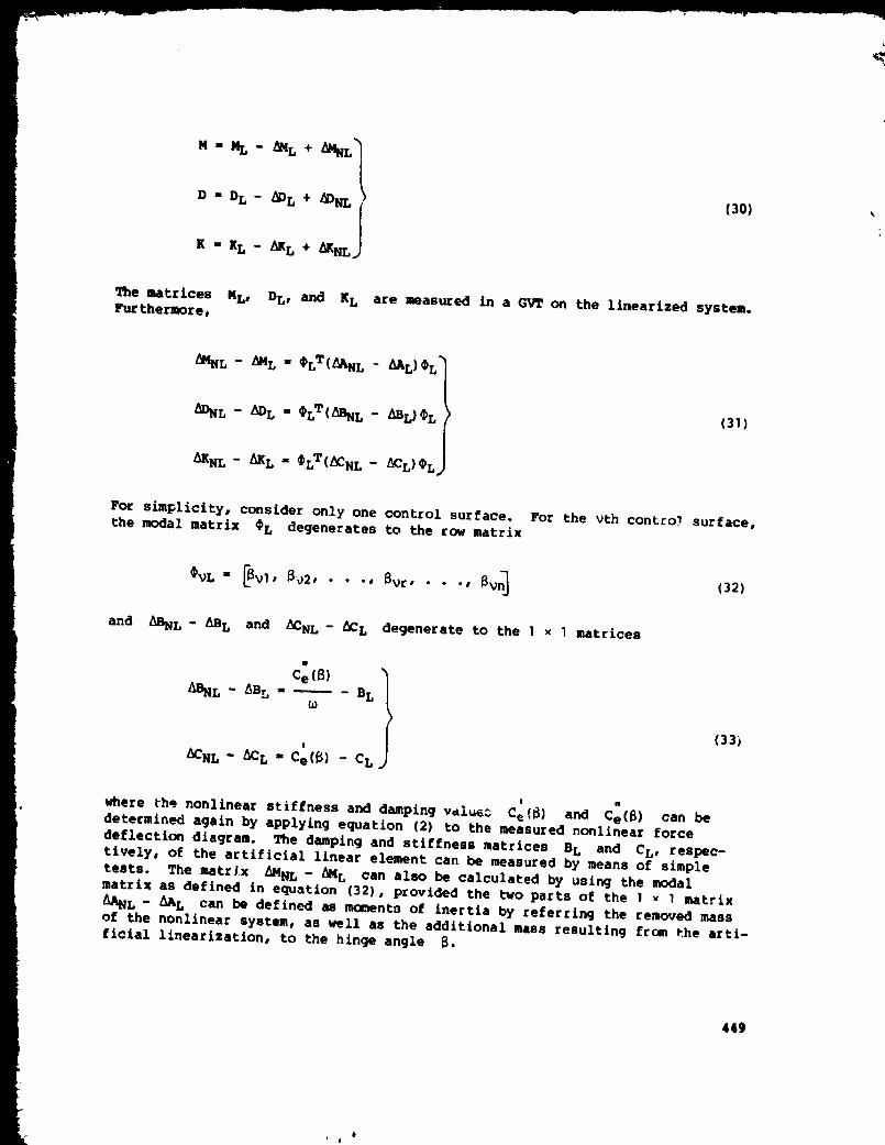
k BThe angles of rotation aar and aar are defined in figure 9. For the specialcase of coupling two systems k and B the c_patibility condition for o

physical degrees of freedom can be expressed by the constraints

A Bg( = u£ - u( = 0 (_, = I, 2, • .., a) (43)

A BIf u_ and u_ are expressed in a series of the normal modes of the systemsA and Be then

nA n B

gR, = u_rqr - u_.rqr = 0

r=l nA+1

(44)

or in matrix notation

g=¥q=O (45)

The aeroelastic equations of motion are defined now by the nk + nB = m gener-alized coordinates. Due to the o constraints there remains a number of

¢ = m - o independent generalized coordinates in terms of which the aero-elastic equations have to be formulated. To do this, the term TT in equa-tion (37) has to be rearranged EOWWiSe SO that

(46)

where T O is a nonsingular o x a matrix. The matrices M, K, D, AK, and_) with respect to both their columns and rows and the column matrix q haveto be rearranged in the same sense. The rearranged equations can be written as

(47)

452

d ! #

where

The new structure of the matrices M, D,

following equation using M as an example

L_e

K, AD, and AK is shown in the

Thus, A can be determined as follows

From equatio,_s (45) and (46) it follows that

(48)

(49)

(50)

qo = -¥_lYcP (51)

Inserting equation (50) into the first c rows of equation (47) and taking intoaccount equation (51) results in the following equation

+ (DIsc + ADcc - (Dco + AD£o.)X - XT(Do._:+ ADoc) + XT(Do0• + ADoo)Xj__

+ {x¢¢ + _cc - (xco + _co)x - xT(_c + _:_c) + xTIr,oa + _oo)x}p " o

(52)

where

X I ¥_1¥c (53)

It can easily be shown that equation (52) can be transformed to the more con-venient equation

453

where

¥T_ + yT(5 + _)y_, + yT(i + Ai)Yp - O (54)

,-E-:J (55)

with the unity matrix I. It should be mentioned that a nonsinqular matrix_a can be determined optimally by applying common mathematical'tools for the

determination of the linear independence of a given number of vectors, as

described, for example, in reference 8. These methods are also applicable

to cases with the nu_er of constraints higher than the rank of matrix TO-Practical applications to structural dynamics problems are presented inreference 9.

It is obvious that the unsteady aerodynamic forces cannot inwaediately becalculated on the basis of the separate normal mode sets of the several sub-structures (main structure and control surfaces). However, this problem caneasily be solved as follows:

(]) Couple the controls to the main structure using the above described

procedure. In doing so, the actual nonlinear stiffnesses Ce are replaced bylinear stiffnesses chosen to be an average representative of the nonlinearO_eS.

(2) Calculate the normal mode characteristics of this linearly coupledsystem and calculate the unsteady aerodynamic forces based oh this set of nor-mal modes.

(3) In the case of hinge stiffness variations or nonlinear flutter cal-

culatlons, the cemblnatlon of concepts III and II described subsequently maybe used.

Combined Application of Concepts I, II, and III

A detailed examinatlon of the possibilities offered by the three conceptsmakes it obvious that scmetiles their cumbined application may be very benefi-cial. Four possible variations can be outlined as follows:

Combination of Concept III and Concept IT:

(1) Apply Concept III, taking into account linear and lightly dampedhinge coupling elements.

(2) Calculate the normal mode characteristics of the linearly coupledsystem.

(3) Vary the linear coupling elements or introduce the nonlinear couplingelements by means of Concept II.

454

4 . $

Esr

C_blnation of Concept III and ConceL_ t T:

(1) Apply Concept III with a completely rigid coupling including the con-

trol hinge degrees of freedom resulting in a configuration with rigidly lockedcontrols.

(2) Take into account the control degrees of freedom according to Concept Iby adding a separate set of control normal modes with the main structure at rest.

Combination of Concept II and Concept t:

(1) Test the aircraft structure with controls removed as a basicconfiguration.

(2) Establish analytically a second configuration with the controls rigidlylocked to the main structure by applying Concept II. This can be achieved byadding modal mass coupling matrices _M to the equations of motion of the basicconfiguration s_ilar to those defined in equation (3|).

When a single control surface is _nsidered the coefficients of the masscoupling matrix AM can be written as

where

_rs " _rT_R_s(56)

@RrT" EUxr ' Uyr, Uzr, rlxr, nyr, nzr3 (57)

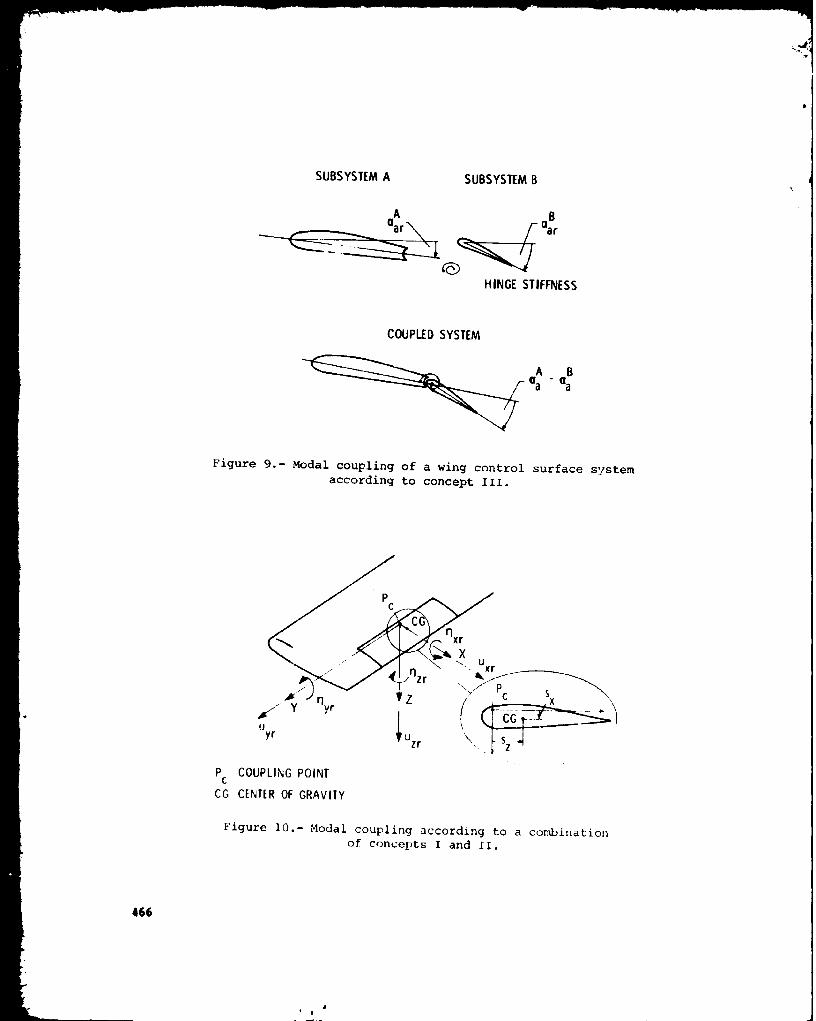
The column matrix %Rr represents the translational and rotational displace-mants at the coupling point of the main structure in relation to the XYZ axis

system (see fig. 10). If the center of gravity of the control lies outside the

coupllr_ point, (Xs, Ys, Zs) = (sx, 0, Sz) , the inertia matrix _AR can bewritten in the forn

mR

O -mRS z O

nasz O -mRs x

0 mRSx 0

O mRSz O -

-mPSz O mRSx

O -mRSx O

IRx + mRsz O -mRSzSx

O IRy • mR(s_ ÷ s_) O

-mRSxSz 0 IR z ÷ mRs_u

d f

(58)

455

where

mR

IRX, IRy, IRZ

mass of the control surface

mass e_ments of inertia of the control surface in

relation to its center of gravity

(3) Take into account the control degrees of freedom according to Concept I

by adding a separate set of control normal modes with the main structure at rest.

Conbination of Concept II and Concept III:

(1) Test the aircraft structure with rigid control dummies in locked con-

dition as a basic configuration. The rigid duemies are used to determine a bet-

ter basic set of normal mode shapes representing the dynamic deformations of

the coupled system than can be determined in the test configuration withremoved controls. This procedure can best be described as convergence accel-

eration by means of interface loading.

(2) Establish analytically a second configuration with the dum_y controls

removed. This can be achieved in accordance with Concept II by subtracting a

modal mass coupling matrix _M as defined in equation (56) from the equations

of motion of the basic configuration.

(3) Apply Concept III coupling the elastic controls to the main structure.

COMPARATIVE CONS ZDERATIONS

The concepts presented offer a nmnber _f possibilities to incorporate th_

control systems of light airplanes, which in general are affected by strong con-

centrated nonlinearities, into the flutter analysis. Special emphasis is placed

on the mathematical modeling of the elastomechanical system based on GVT. It

is obvious that a final evaluation of the applicability and accuracy of the dif-

ferent concepts is rather difficult because, up to the present time, only

Concept I has been applied to some extent to real airplane structures. Only

little experience with the other concepts is at hand. Thus, Concept II has

recently been employed in the course of the flutter clearance process of the

soaring alrplane ASW-]5. Flutter calculations based on this concept predicted

tail flutter at about 200 km/hr. That result was verified by flight flutter

tests, where the airplane showed nonlinear flutter in a speed range from

]75 to 220 km/hr, starting with comparably small amplitudes at ]75 km/hr and

increasing to very high amplitudes far beyond the regular rudder stroke at

higher speeds. This behavior in concurrence with substantial alterations of

the flutter modes is symptomatic of highly nonlinear flutter cases. A mo_e

detailed consideration of this special problem exceeds the subject of this

paper and should be reserved for fur ther investigations.

It is also worth mentioning that the ground vibration test carried out in

accordance with this concept to_ far less test time than a normal test on the

unchanged structure (reduction of about e0_).

456

The first comparative investigation of the Concepts I, II, and III has

been the special concern of reference 10, where results are reported £or a

simple plate-type wing-aileron model with largely linear elastodynamical prop-

erties. Although this model cannot be considered representative in all respects

of the elastodynamical behavior of real airplanes, it seems to be opportune to

use the results of this investigation together with the present experience with

the Concepts I and II as a basis for a preliminary assessment concerning the

advantages and the weak points of different methods. For this purpose a selected

number of criteria is used taking into consideration several requirements such

as

(]) Test effort required

(2] Numerical effort required

(3) General applicability

(4) Physical consistency

Table ] shows in a condensed form how the criteria are met by the several

concepts.

%

CONCLUDING REMARKS

It has been known for many years that the flutter clearance of light air-

planes can be highly afflicted by uncertainties stemming from strong localized

nonlinearities in the control mechanisms. It is shown that the establishment

of more reliable and accurate mathematical models for the flutter analysis

requires modified ground vibration test procedures combined with suitably

adapted modal synthesis approaches. Three basic concepts with several varia-

tions have beer _escribed in detail. They offer a diverse choice of tools for

carrying out Loth approximately linearized and nonlinear flutter investigations.

A comparative consideration has been made as to the capacity as well as

the drawbacks of the different concepts. However, because of lack of practical

experience with Concepts II and III, it is not possible at present to make a

conclusive evaluation.

457

REFACES

]. Breitbach, E.: Effects of Structural Non-Linearities on Aircraft Vibration

and Flutter. AGARD Report No. 665, Sept. ]977.

2. Dat, R.; Tretout, R.| and Lafont, J. M.: Eassais de Vibration d'une Struc-P 0

ture Cumportant du Frottement Sec. La Rech. Aerospatzale, No. 3, 1975,

pp. ]69-]74.

3. Bogoljubow, N. N.; and Mitropolski, J. A.: Asymtotische Methoden in der

Theorie der nichtlinearen Schwingungen. Akademie-Verlag, Berlin, ]965.

4. Scanlan, R. H.; and Rosenbaum, R.: Introduction to the Study of Aircraft

Vibration and Flutter. MacMillan Co., ]95].

5. Kussner, H. G.| and GSllnitz, H.: Theorie und Methode der Flatterrechnung

yon Flugzeugen unter Benutzung des Standschwingungsversuchs. AVA-

Forschungsbericht 64-0], ]964.

6. Kussner, H. G.; and Breitbach, E.: Bestimmung der Korrekturglieder der

Bewegungsgleichungen bei Aenderungen eines elastomachanischen Systems.

AVA-Report 69 J 01, ]969.

7. Breitbach, E.: Investigation of Spacecraft Vibrations by Means of the Modal

Synthesis Approach. ESA-SP-12], Oct. 1976, pp. ]-7.

8. Courant, R.; and Hilbert, I.: Methoden der mathematischen Physik I. Heidel-

berger Taschenb_cher, Springer-Verlag, ]968.

9. Walton, W. C.; and Steeves, E.C.: A New Matrix Theorem and Its Application

for Establishing Independent Coordinates for Complex Dynamical Systems With

Constraints. NASA TR R-326, ]969.

]0. H_ners, H.: Ser_cksichtigung der Ruder_eiheitsgrade im Flatternachweis yon

Flugzeugen. DFVLR-Report IB 253-78 J 07, 1978.

458

&i-i

&

rj

It40

E-_

U3

iI

I

;-t u,.i .aJ _.

I_ -,,,4 I,,,i ",,',10

'-'".-, _i,-.-, -,,-,I 0

p_, |'_aa Ill r" -,..4

eu,l_

t

e. ,._

•_,_ _ o- U _

_Ig ,, &

!

r.

0 la "I

i-4

P,t I_ lU_'t

0

I

@I,l

I0

4;,=4

I_l

s., I "

-,-I :::l

rj

_v,.i

m r_

1

0 _

o,, ._-_

• _

I ,"4 !t "_

!

Ill I II,-I

_o _,_,_

I_ o,-t

_ •

-_ _ o

_,_ _,._

,-4 I_

"_,_

.Q _1 0 •4J _a

o _ _

""_ M

I0 @ I_

I "'_ a.I r,.

_.._' .,-I 4,,__1,-I

"' 0 "0

2

0

!

•_ _ 0

•..i ._ .',

1

e_ ,-.t

_o_1,4 I,,I

I I

0 cn

•,,,I _

o_

¢.,°.4

,.4 _ _ I _"

• r, I-_

w

.IJ

_p

.,-4

0O

459

Figure i.- Schematical sketch of the control system of a light airplane.

460

RUDDERHINGE

MOMENT,N-m

0

-5i

-I0-40

I

I ,I

-2L) 0 20

RUDDERHINGE ANGLE._,. clecj

(a) Force deflection diagram.

J

40

RUDDERHINGE

STIFFNESS.I

Ce(1)),

N-m

1.5 x 102

!_-DAMPING I

SS I.5 i

r

I0 30 60

RUDDERHINGE ANGLE,p. cleq

DAMPING

DECREMENT.C'(3)

(b) Hinge stiffness and damping versus hinge an%le.

Figure 2.- Force deflection diagram and stiffness and <|ampi_g

for the rudder system of a scaring airplane.

461

, # •

AILERONHINGE

MOMENT. N-m

ANTISYMMETRICALCASE

-10 0 l0AILERON HINGE ANGLE,

I).(_

I I2O

(a) Force deflection diagram.

3

AILERONHINGESTIFFNESS, 2

c'Jls),

N-m l

" x 102 0.4

I

, l 1I0 20 30

AILfRON HINGE ANGLE.£ deg

DAMPINGDECREMENT,

Ce'_

6-rr_

ANTIS'¢MMETRICALCASE

(b) Hinge stiffness and damping versu_ hinge angle.

Figure 3.- Force deflection diagram and stiffness a_id damEing fc>r

the aileron system of & soaring airplane. Antis%_nmetrical _a_e.

462

0 -

10-

AILERON ItlNGE

MOMENT. 0N-m

-10

-20-2

SYMMEIRICAL CASE

I-! 0

AILERON HINGE ANGLE.

I_,d_

(a) Force deflection diagram.

AILERON 2H INGESTIFFNESS,

c'_,N-m |

_lo4

_ / , cAs/SYM_ETRIECAL J

1 ?

AILERON HINGE ANGLE.

B. _ecj

(,,b)Hinge stiffness _,d damping versus hinge angle.

Figure 4.- Force deflection diagram and stiffness and damping for

the aileron system of a soaring airplane. Symmetrical case.

463

' r

10

AILERON

HINGE 5ANGLE,B. _eg

10

BACKLASH

PRING TA81

ZO 30

FLUTTERSPEED.VF. mlsec

F = 0.13 N-mO

_o = 1"3°

C] = 4.7 N-m

C2 = 16 N-m

Figure 5.- Measured flutter boundary of a nonlinear model.

®By

NORMAL MODE WITHCONTROLSURFACELOCKED

NORMAL MODEWITH LIFTINGSURFACEAT RESTANDCONTROLSURFACEFREE

ARBITRARY DEFLECTION

Figure 6.- Modal superposition according to concept I.

Controls without tabs.

464

L '.

I h C,G.OFCONTROL-

__AB SYSTEM

c.o.o,ON,C. G. OF THE TAB _

Figuze 7.- Lifting surface with control surface and tab.

NORMA!. MODE WITH CS AND

T LOCKED

NORMAL MODEWITH CS FREE

T LOCKED.AND LS AT REST

C.--.--_----.7,e--,.,._ (1)Cv NORMAL MODE WITH CS LOCKED,

T FREE. AND LS AT REST

UARBITRARY DEFLECTION

LS: LIFTINGSUR:ACE

CS: CONTROL SURFACE

T:TAB

Figure 8.- Modal superposition according to concept I.Controls with tabs.

46S

i f 4

SUBSYSTEM A SUBSYSTEM B

HINGE STIFFNESS

COUPLED SYSTEM

A B

aa - a a

Figure 9.- Modal coupling of a wing control surface system

according to concept Ill.

Pc

.P3 _/ I - "--_/ P , \

.4_n vz / , c ._x \.

!Uyr I Uzr \\.

P COUPLING POINTc

CG CENTER OF GRAVITY

Figure I0.- Modal coupling according to a combination

of concepts I and II.

466

, !

ADVANCED C0tqPOSITES IN SAILPLANE STRUCTURES:

APPLICATION AND MECHANICAL PROPERTIES

Dieter Muser

Research Center Stuttgart

Deutsche Forschungs- und Versuchsanstalt

f_r Luft- und Raumfahrt e.V.

SmeU_Y

Advanced Composites in Sailplanes mean the use of carbon and aramid fib-

ers in an epoxy matrix. Weight savings are in the range of 8 to 18% in compar-

ison with glass fiber structures. The laminates will be produced by hand-layup

techniques and all material tests shown here have been done with these mate-

rials. These values may be used for calculation of strength and stiffness as

well as for comparison of the materials to get a weight-optimum construction.

Proposals for materlal-optimum construction are mentioned.

TECHNICAL HISTORY

The first fiber-reinforced glider, a Phoenix developed by Prof. Eppler,

made its maiden flight in 1957. Now, more than 4000 gliders with glass-fiber-

reinforced structures are in the air all over the world. Increasing the wing

loading permitted increases in maximum speed, but structural demands increased

the weight also.

A large span enabled the constructors to build planes with lift to drag

ratios of about 50 (ASW 17z 48.5, Nimbus 2: 49) and sinking speeds of 0.50 m/s

(].64 it/s). But it was not possible to realize wing spans with more than

22 maters without a very soft win_ structure. This was possible when carbon

fibers were used in the center wing section of the Akaflieg Braunschweig SB I0

in 1972 (fig. 1). Wlth a maximum wing span of 29 meters, this glider has the

best glide ratio of 53 and a sinking speed of 0.41 m/s (].35 it/s). But the

price of carbon fibers was very high at this tima and so this material was used

only in another prototype, the Akaflleg Stuttgart is-29 in 1975. To realize

the old dream to vary the span during flight, it was absolutely necessary to

use carbon fibers in the outer moving part of the wing and in the spar of the

inner wing section. When the Akaflieg Braunschweig built the first all-carbon

gllder in 1977/78, they used carbon fibers to reduce weight dnd to stiffen the

wing, so that all flaps move only very slightly and the pilot is able to han-

dle them. And this was the year when carbon fibers were used in a larger vol-

uma in different types of commercial gliders.

467