1A Sparsity-driven Approach for Joint SAR

Imaging and Phase Error CorrectionN. OzbenOnhon and Mujdat Cetin

Faculty of Engineering and Natural Sciences, Sabancı University, Orhanlı, Tuzla, 34956

Istanbul, Turkey

Abstract

Image formation algorithms in a variety of applications have explicit or implicit dependence on

a mathematical model of the observation process. Inaccuracies in the observation model may cause

various degradations and artifacts in the reconstructed images. The application of interest in this paper

is synthetic aperture radar (SAR) imaging, which particularly suffers from motion-induced model errors.

These types of errors result in phase errors in SAR data whichcause defocusing of the reconstructed

images. Particularly focusing on imaging of fields that admit a sparse representation, we propose a

sparsity-driven method for joint SAR imaging and phase error correction. Phase error correction is

performed during the image formation process. The problem is set up as an optimization problem in a

nonquadratic regularization-based framework. The methodinvolves an iterative algorithm each iteration of

which consists of consecutive steps of image formation and model error correction. Experimental results

show the effectiveness of the approach for various types of phase errors, as well as the improvements it

provides over existing techniques for model error compensation in SAR.

Index Terms

Synthetic aperture radar, phase errors, autofocus, regularization, sparsity.

I. I NTRODUCTION

Synthetic aperture radar (SAR) has recently been and continues to be a sensor of great interest in

a variety of remote sensing applications, in particular because it overcomes certain limitations of other

This work was partially supported by the Scientific and Technological Research Council of Turkey under Grant 105E090,

and by a Turkish Academy of Sciences Distinguished Young Scientist Award.

July 6, 2011 DRAFT

sensing modalities. First, SAR is an active sensor using its own illumination. To illuminate a ground

patch of interest, the SAR sensor uses microwave signals which provide SAR with the capability of

imaging day and night as well as in adverse weather conditions. Due to these features of SAR, SAR

image formation has become an important research topic. The problem of SAR image formation is a

typical example of inverse problems in imaging. Solution of inverse problems in imaging requires the

use of a mathematical model of the observation process. However such models often involve errors and

uncertainties themselves. As a predominant example in SAR imaging, motion-induced errors are reasons

for model uncertainties which may cause undesired artifacts in the formed imagery. This type of errors

causes phase errors in the SAR data which result in defocusingof the reconstructed images [1]. Because

of the defocusing effect of such errors, the techniques developed for removing phase errors are often

called autofocus techniques.

Various studies have been presented on the SAR autofocus problem [2–17]. One of the most well

known techniques, Phase Gradient Autofocus (PGA) [2], estimates phase errors using the data obtained

by isolating many single defocused targets via center-shifting and windowing operations. It is based on

the assumption that there is a single target at each range coordinate. Another well-known approach for

autofocus is based on the optimization of a sharpness metricof the defocused image intensity [3–10].

These techniques aim to find the phase error estimate which minimizes or maximizes a sharpness function

of the conventionally reconstructed image. Commonly used metrics are entropy or square of the image

intensity. Techniques such as mapdrift autofocus [11] use subaperture data to estimate the phase errors.

These techniques are suitable mostly for quadratic and slowly varying phase errors. A recently proposed

autofocus technique, multichannel autofocus (MCA) [12], is based on a non-iterative algorithm which

finds the focused image in terms of a basis formed from the defocused image, relying on a condition on

the image support to obtain a unique solution. In particular, MCA estimates 1D phase error functions by

directly solving a set of linear equations obtained throughan assumption that there are zero-reflectivity

regions in the scene to be imaged. When this is not precisely satisfied, presence of a low-return region is

exploited, and the phase error is estimated by minimizing the energy of the low-return region. When the

desired conditions are satisfied, MCA performs very well. However, in scenarios involving low-quality

data (e.g., due to low SNR) the performance of MCA degrades. A number of modifications to MCA

have been proposed, including the incorporation of sharpness metric optimization into the framework

[12], and the use of a semidefinite relaxation based optimization procedure [17] for better phase error

estimation performance.

2

One common aspect of all autofocus techniques referred to above is that they perform post-processing,

i.e., they use conventionally reconstructed (i.e., reconstructed by the polar-format algorithm [18, 19])

defocused images in the process of phase error estimation. Our starting point however is the observa-

tion that more advanced SAR image formation techniques have recently been developed. Of particular

interest in this paper is regularization-based SAR imaging (see, e.g., [20–22]), which has been shown

to offer certain improvements over conventional imaging. Regularization-based techniques can alleviate

the problems in the case of incomplete data or sparse apertures. Moreover, they produce images with

increased resolution, reduced sidelobes, and reduced speckle by incorporation of prior information about

the features of interest and imposing various constraints (e.g., sparsity, smoothness) about the scene.

However, existing regularization-based SAR imaging techniques rely on a perfect observation model, and

do not involve any mechanism for addressing any model uncertainties.

Motivated by these observations and considering scenes that admit sparse representation in some

dictionary, we propose a sparsity-driven technique for joint SAR imaging and phase error correction by

using a nonquadratic regularization-based framework. In the proposedsparsity-driven autofocus (SDA)

method, phase errors are considered as model errors which are estimated and removed during image

formation. The proposed method handles the problem as an optimization problem in which the cost

function is composed of a data fidelity term (which exhibits a dependence on the model parameters) and

a regularization term, which is thel1 − norm of the field. For simplicity we consider scenes that are

spatially sparse, however our approach can be applied to fields that are sparse in any given dictionary

by using anl1 − norm penalty on the associated sparse representation coefficients. The cost function

is iteratively minimized with respect to the field and the phase error using coordinate descent. In the

first step of every iteration, the cost function is minimized with respect to the field and in the second

step the phase error is estimated given the field estimate. The phase error estimate is used to update the

model matrix and the algorithm passes to the next iteration.To the best of our knowledge, this work

is first in the context of providing a solution to the problem ofmodel errors in sparsity-driven image

reconstruction.

Sharpness-based autofocus techniques [3–10] share certainaspects of our perspective, but our approach

is fundamentally different. In particular, our approach also involves a certain type of sharpness metric

about the field, but inside of a cost function as a side constraint (regularization term) to a data fidelity term

which incorporates the system model and the data into the optimization problem for image formation.

Hence our approach imposes the sharpness-like constraint during the process of image formation, rather

3

than as post-processing. This enables our technique to correct for artifacts in the scene due to model errors

effectively, in an early stage of the image formation process. Furthermore, unlike existing sharpness-based

autofocus techniques, our model error correction approachis coupled with an advanced sparsity-driven

image formation technique which has the capability of producing high resolution images with enhanced

features, and as a result our approach is not limited by the constraints of conventional SAR imaging. In

fact, our approach benefits from a dual use of sparsity, both for model error correction (autofocusing)

and for improved imaging. Finally, our framework is not limited to sharpness metrics on the scene, but

can in principle be used for model error correction in scenesthat admit a sparse representation in any

given dictionary.

We present results on synthetic scenes as well as on two public datasets. Qualitative as well as

quantitative analysis of the experimental results shows the effectiveness of the proposed method and

the improvements it provides over existing methods in termsof both scene reconstruction as well as

phase error estimation.

The rest of this paper is organized as follows. In Section II, the observation model for a SAR imaging

system is described. In Section III, a general view of the phase errors and their effect on the SAR data

are provided. In Section IV, the proposed method is describedin detail and in Section V the experimental

results are presented. We conclude the paper in Section VI andprovide some technical details in the

Appendix.

II. SAR OBSERVATION MODEL

In SAR systems, one of the most widely used signals in transmission is the chirp signal:

s(t) = Re{

e[j(ω0t+αt2)]}

(1)

Here,ω0 is the center frequency and2α is the so-called chirp-rate. For spotlight-mode SAR, which is the

modality of interest in this paper, the received signalqm(t) at them− th aperture position (cross-range

position) involves the convolution of the transmitted chirp signal with the projectionpm(u) of the field

at that aperture position.

qm(t) = Re

{∫

pm(u)ej[ω0(t−τ0−τ(u))+α(t−τ0−τ(u))2]du

}

(2)

pm(u) =

∫ ∫

x2+y2≤L2

δ (u − x cos θ − y sin θ)F (x, y)dxdy (3)

4

Here,L is the radius of the circular patch to be imaged,F (x, y) denotes the underlying field and,θ is

the observation angle at them − th aperture position. If we let the distance from the SAR platform to

the center of the field bed0, then τ0 + τ(u) is the delay for the returned signal from the scatterer at

the range positiond0 + u, whereτ0 is the demodulation time. The data used for imaging are obtained

after a pre-processing step. From the projection-slice theorem [23], the SAR datarm(t) obtained after

this pre-process, can be identified as a band-pass filtered Fourier transform of the projections of the field

[24],

rm(t) =

∫

|u|≤L

pm(u)e−jUudu (4)

where

U =2

c(ω0 + 2α(t − τ0)) (5)

Substituting (3) into (4), we obtain the relationship between the observed datarm(t) and the underlying

field F (x, y).

rm(t) =

∫ ∫

x2+y2≤L2

F (x, y)e−jU(x cos θ+y sin θ)dxdy (6)

All of the returned signals from all observation angles constitute a patch from the two dimensional spatial

Fourier transform of the corresponding field. These data are called phase histories and lie on a polar grid

in the 2D frequency domain as shown in Figure 1. Let the 2D discrete phase history data be denoted by

a K × M matrix R. Columnm of R, denoted by theK × 1 vector rm, is obtained by samplingrm(t)

(the returned signal at cross-range positionm), in fast-timet (range direction) atK positions. In terms

of this notation, the discrete observation model can be formulated as follows [20]:

r1

r2

rM

︸ ︷︷ ︸

rMK×1

=

C1

C2

CM

︸ ︷︷ ︸

CMK×I

fI×1 (7)

Here, the vectorr of observed samples is obtained just by concatenating the columns of the 2D phase

history dataR, under each other.Cm andC are discretized approximations to the continuous observation

5

Fig. 1. Graphical representation of an annulus segment containing known samples of the phase history data in the 2D frequency

domain.

kernel at the cross-range positionm and for all cross-range positions, respectively.f is a vector repre-

senting the sampled and column-stacked version of the reflectivity image F (x, y). Note thatK andM

are the total numbers of range and cross-range positions, respectively.

III. PHASE ERRORS

During the pre-processing of the SAR data (mentioned in Section II), the demodulation timeτ0 needs

to be known. When this time is known imperfectly, the SAR data obtained after pre-processing contain

phase errors. The inexact knowledge of the demodulation timeoccurs when the distance between the SAR

sensor and the scene center cannot be determined perfectly due to SAR platform position uncertainties

or when the signal has delay due to some atmospheric effects.Since uncertainties on, e.g., the position

of the platform are constant over a signal received at one aperture position but are different at each

aperture position, phase errors caused by such uncertainties vary only along the cross-range direction

in the frequency domain. The implication of such an error in the image domain is the convolution of

(each range line of) the image with a 1D blurring kernel in thecross-range direction. Hence, such phase

errors cause defocusing of the image in the cross-range direction. An example of SAR platform position

uncertainties arises from errors in measuring the aircraftvelocity. A constant error on aircraft velocity

6

induces a quadratic phase error function in the data [1]. Usually, phase errors arising due to SAR platform

position uncertainties are slowly-varying (e.g., quadratic, polynomial) phase errors, whereas phase errors

induced by propagation effects are much more irregular (e.g., random ) phase errors [1]. While most

phase errors encountered are 1D cross-range varying functions, it is possible to encounter both range

and cross-range varying 2D phase errors as well. For instance, in low frequency UWB SAR systems,

severe propagation effects may appear through the ionosphere, including Faraday rotation, dispersion, and

scintillation [25] which cause 2D phase errors, defocusingthe reconstructed image in both range and cross-

range directions. Moreover, waveform errors such as frequency jitter from pulse to pulse, transmission line

reflections and waveguide dispersion effects may cause defocus in both range and cross-range direction

[18]. 2D phase errors can in principle be handled in two sub-categories as separable and non-separable

errors, but it is not common to encounter 2D separable phase errors in practice.

For these three types of phase error functions, let us investigate the relationship between the phase-

corrupted and error-free phase history data in terms of the observation model.

A. 2D Non-separable Phase Errors

In the presence of 2D non-separable phase errors, all samplepoints of theK ×M phase history data

are perturbed with different and potentially independent phase errors. LetΦ2D−ns be a 2D non-separable

phase error function. The relationship between the phase-corrupted and error-free phase histories are as

follows:

Rε(k, m) = R(k, m)ejΦ2D−ns(k,m) (8)

Here, Rε denotes the phase-corrupted phase history data. To expressthis relationship in terms of the

observation model, first we define the vectorφ2D−ns

φ2D−ns =

[

φ2D−ns(1), φ2D−ns(2), ..., φ2D−ns(S)

]T

(9)

which is created by concatenating the columns of the phase error matrixΦ2D−ns under each other. Here,

S is the total number of data samples and equal to the productMK. Using the corresponding vector

forms, the relationship in (8) becomes

rε = D2D−nsr (10)

whereD2D−ns is a diagonal matrix:

D2D−ns = diag

[

ejφ2D−ns(1), ejφ2D−ns(2), ..., ejφ2D−ns(S)

]

(11)

7

In terms of observation model matrices, the relationship in(10) is as follows

C (φ2D−ns) f = D2D−nsCf (12)

where,C is the initially assumed model matrix by the imaging system and C (φ2D−ns) is the model

matrix that takes the phase errors into account. The equations (10) and (12) can be expressed in the

following form as well.

rε(s) = ejφ2D−ns(s)r(s) (13)

Cs (φ2D−ns) f = ejφ2D−ns(s)Csf for s = 1, 2, ....., S

Here,r(s) denotess − th element of the vectorr andCs denotess − th row of the model matrixC.

B. 2D Separable Phase Errors

A 2D separable phase error function is composed of range varying and cross-range varying 1D phase

error functions as follows:

Φ2D−s(k, m) = ξ(k) + γ(m) (14)

Here,ξ, representing the range varying phase error, is aK×1 vector andγ, representing the cross-range

varying phase error, is aM ×1 vector. TheS×1 vector for 2D separable phase errorsφ2D−s, is obtained

by concatenating the columns ofΦ2D−s as follows:

φ2D−s =

[

ξ(1) + γ(1)︸ ︷︷ ︸

φ2D−s(1)

, ..., ξ(K) + γ(1)︸ ︷︷ ︸

φ2D−s(K)

, ξ(1) + γ(2)︸ ︷︷ ︸

φ2D−s(K+1)

, ..., ξ(1) + γ(M)︸ ︷︷ ︸

φ2D−s((M−1)K+1)

, ..., ξ(K) + γ(M)︸ ︷︷ ︸

φ2D−s(S)

]T

(15)

A 2D separable phase error function affects the observationmodel matrix in the following manner:

rε = D2D−sr (16)

C (φ2D−s) f = D2D−sCf

Here,D2D−s is a diagonal matrix:

D2D−s = diag

[

ejφ2D−s(1), ejφ2D−s(2), ..., ejφ2D−s(S)

]

(17)

8

C. 1D Phase Errors

We mentioned before that most encountered phase errors are functions of cross-range only. In other

words, for a particular cross-range position the phase error is same at all range positions. Letφ1D be the

1D cross-range varying phase error.φ1D is a vector of lengthM :

φ1D =

[

φ1D(1), φ1D(2), ..., φ1D(M)

]T

(18)

In the case of 1D phase errors, the relationship between the error-free and the phase-corrupted data can

be expressed as:

rε = D1Dr (19)

C (φ1D) f = D1DCf

Here,D1D is a S × S diagonal matrix defined as:

D1D = diag

[

ejφ1D(1), ejφ1D(1), ..., ejφ1D(1)

︸ ︷︷ ︸

K

ejφ1D(2), ..., ejφ1D(2)

︸ ︷︷ ︸

K

, ejφ1D(3), ..., ejφ1D(M), ..., ejφ1D(M)

︸ ︷︷ ︸

K

]

(20)

These relationships can also be stated as follows:

rεm= ejφ1D(m)rm (21)

Cm (φ1D) f = ejφ1D(m)Cmf for m = 1, 2, ....., M

Here, rm and Cm are the error-free phase history data and the assumed model matrix for the m − th

cross-range position. Note that, in a 1D cross-range phase error case, there areM unknowns, in a 2D

separable phase error case there areM +K unknowns, and in a 2D non-separable phase error case there

areS = MK unknowns. Hence, correcting for 2D non-separable phase errors is a much more difficult

problem than the others.

IV. PROPOSEDMETHOD

In conventional imaging, the image is formed by interpolating the SAR data from the polar grid to a

rectangular grid and then taking its 2D inverse Fourier transform. Images formed by conventional imaging

usually suffer from speckle and sidelobe artifacts. Furthermore the resolution of the images is limited

by the SAR system bandwidth. On the other hand, we know that regularization-based image formation

techniques can deal with these problems and they have been succesfully applied to SAR imaging. These

techniques formulate image formation as an optimization problem. The cost function is composed of a

least-squares data fidelity term, as well as a side constraintor regularization term which incorporates

9

information about the structure of the scene (sparsity, smoothness etc.) into the optimization problem.

Incorporation of prior information about the scene provides feature enhanced images with increased

resolution, reduced sidelobes, and reduced speckle. In thecontext of SAR imaging of man-made objects,

the underlying scene, dominated by strong metallic scatterers, is usually sparse, i.e., there are few nonzero

pixels. To impose sparsity, often nonquadratic side constraints are incorporated into the cost function.

There are a variety of nonquadratic terms to use as the side constraint. The general family oflp−norms

is one of them. Althoughl0 − norm is in principle, theright choice to obtain sparse solutions, using

l0 − norm results in a combinatorial optimization problem. Therefore, generally, instead ofl0 − norm,

l1−norm of the field is used to obtain sparse solutions. Usingl1−norm of the field results in a convex

optimization problem which is easier to solve. Moreover, recently it has been shown that under certain

conditions,l0 − norm and l1 − norm yield identical solutions [26]. This observation has sparked much

recent interest both in theory and in applications of sparserepresentations, coverage of which is beyond

the scope of this paper.

Sparsity-driven radar imaging has already found use in a number of contexts [27–39]. In SAR applica-

tions, there is widespread use of sparsity-based imaging due to the advantages such as super-resolution and

artifact suppression it provides. Such techniques assume that the observation model is known exactly.

In the presence of phase errors and an additive measurement noise induced by the SAR system, the

observation model becomes

g = C(φ)f + v (22)

wherev stands for measurement noise, which is assumed to be white Gaussian noise (the most com-

monly used statistical model for radar measurement noise [40, 41]), andg is the noisy phase-corrupted

observation data. Here,φ refers to one of the three types of phase errors introduced inSection III.

Based on these observations we propose a nonquadratic regularization-based method for joint imaging

and phase error correction. While existing sparsity-driven SAR imaging methods assume that data contain

no phase errors, our approach jointly estimates and compensates such errors in the data, while performing

sparsity-driven image formation. In particular, we pose the joint imaging and phase error estimation

problem as the problem of minimizing the following cost function:

J(f, φ) = ‖g − C(φ)f‖22 + λ ‖f‖1 (23)

Here,λ is the regularization parameter, which specifies the strength of the contribution of the regular-

ization term into the solution. The given cost function is minimized jointly with respect tof and φ

10

using coordinate descent technique. The algorithm is an iterative algorithm, which cycles through steps

of image formation and phase error estimation and compensation. Every iteration involves two steps. In

the first step, the cost function is minimized with respect to the field and in the second step the phase

error is estimated given the field estimate. Before the algorithm passes to the next iteration, the model

matrix is updated using the estimated phase error. This flow is outlined in Algorithm 1.

In Algorithm 1, n denotes the iteration number.f (n) and φ(n) are the image and phase error estimates

at iterationn, respectively. Note that the knowns in this algorithm are the noisy phase-corrupted datag

and the initially assumed model matrixC. The unknowns are the fieldf and the phase errorφ together

with the associated model matrixC(φ) that takes the phase errors into account. It is worth noting here

Algorithm 1 Algorithm for the Proposed SDA Method

Initialize n = 0 f (0) = CHg andC(φ(0)) = C

1. f (n+1) = arg minf J(f, φ(n))

2. φ(n+1) = arg minφ J(f (n+1), φ)

3. UpdateC(φ(n+1)) using φ(n+1) andC.

4. Let n = n + 1 and return to 1.

Stop when∥∥∥f (n+1) − f (n)

∥∥∥

2

2/

∥∥∥f (n)

∥∥∥

2

2is less than a pre-determined threshold.

In this paper, the value of the threshold is chosen as10−3.

that the use of the nonquadratic regularization-based framework contributes to the accurate estimation

of the phase errors as well. Although nonquadratic regularization by itself cannot completely handle the

kinds of phase errors considered in this work, it exhibits some robustness to small perturbations on the

observation model matrix [42]. In the context of our approach, the nonquadratic regularization term in the

cost function provides a small amount of focusing of the estimated field in each iteration. This focusing

then enables better estimation of the phase error. This in turn results in a more accurate observation

model matrix, which provides better data fidelity and leads toa better field estimate in the next iteration.

Next, we provide the details of the algorithm for the three classes of phase errors described in Section

III.

11

A. Algorithm for 1D Phase Errors

In the algorithm for 1D phase errors, in the first step of every iteration the cost functionJ(f, φ1D) is

minimized with respect tof . This is the image formation step and same for all types of phase errors.

f (n+1) = arg minf

J(f, φ(n)1D) = arg min

f

∥∥∥g − C(φ

(n)1D)f

∥∥∥

2

2+ λ ‖f‖1 (24)

To avoid problems due to nondifferentiability of thel1 − norm at the origin, a smooth approximation is

used [20]:

‖f‖1 ≈I∑

i=1

(|fi|2 + β)1/2 (25)

whereβ is a nonnegative small constant. In each iteration, the field estimate is obtained as

f (n+1) =(

C(φ(n)1D)HC(φ

(n)1D) + λW (f (n))

)−1C(φ

(n)1D)Hg (26)

whereW (f (n)) is a diagonal matrix:

W (f (n)) = diag

1

(∣∣∣f

(n)i

∣∣∣

2+ β)1/2

..................1

(∣∣∣f

(n)I

∣∣∣

2+ β)1/2

(27)

The matrix inversion in (26) is not carried out explicitly, but rather numerically through the conjugate

gradient algorithm. Note that, this algorithm has been usedin a variety of settings for sparsity-driven

radar imaging, and has been shown to be a descent algorithm [43].

The second step involves phase error estimation, in which a different procedure is implemented for

each type of phase errors. For 1D cross-range varying phase errors, given the field estimate, the following

cost function is minimized for every cross-range position [44],

φ(n+1)1D (m) = arg min

φ1D(m)J(f (n+1), φ1D(m)) = arg min

φ1D(m)

∥∥∥gm − e(jφ1D(m))Cmf (n+1)

∥∥∥

2

2(28)

for m = 1, 2, ...., M

whereφ(n+1)1D (m) denotes the phase error estimate for the cross-range position m in the iteration(n+1).

In (28), theK × 1 vector gm is the noisy SAR data at them− th cross-range position. After evaluatingthe norm expression in (28) (see appendix for details), we obtain

φ(n+1)1D

(m) = arg minφ1D(m)

(

gHm gm − 2

√

<2 + =2 cos

[

φ1D(m) + arctan

(−=

<

)]

+ f (n+1)H

CHm Cmf (n+1)

)

(29)

where

< = Re{

f (n+1)H

CHm gm

}

= = Im{

f (n+1)H

CHm gm

}

(30)

12

We know that negative cosine has its minimum at zero and integer multiples of 2π, so if we set the

argument of the cosine to zero, we can find the phase error estimate in closed form as given in (31) for

the corresponding aperture position.

φ(n+1)1D (m) = − arctan

(−=

<

)

(31)

Using the phase error estimate, the model matrix is updated as follows:

Cm(φ(n+1)1D (m)) = e(jφ

(n+1)

1D(m))Cm for m = 1, ...., M (32)

We incrementn and turn back to the optimization problem in (24).

Moreover, note that, phase updates are performed after eachstep of the f-iteration in (26), as a result of

which, the overall computational load of our approach is notsignificantly more than that of just image

formation.

B. Algorithm for 2D Separable Phase Errors

In case of 2D separable phase errors, the field estimate is obtained via minimizing the following cost

function:

f (n+1) = arg minf

J(f, φ(n)2D−s) = arg min

f

∥∥∥g − C(φ

(n)2D−s)f

∥∥∥

2

2+ λ ‖f‖1 (33)

Given the field estimate, first, the phase error in the cross-range direction,γ, is estimated using the 1D

phase error estimation procedure described in Section IV.A,and then this estimate is used to update the

model matrix as follows:

γ(m)(n+1) = arg minγ(m)

J(f (n+1), γ(m)) = arg minγ(m)

∥∥∥gm − e(jγ(m))Cmf (n+1)

∥∥∥

2

2(34)

for m = 1, 2, ...., M

Cm(γ(m)(n+1)) = e(jγ(m)(n+1))Cm for m = 1, 2, ...., M (35)

Then, to estimate the phase error in the range direction, the elements of the data vectorg and the rows of

the model matrixC(γ(n+1)) are ordered in such a way that the elements and rows corresponding to the

same range position lie under each other. Let these modified data vector and modified model matrix be

gmod andCmod, respectively. (i.e., the phase history matrix is row-stacked rather than column-stacked.)

13

Using these new variables, the phase error estimateξ for the range direction is found repeating the same

procedure as in cross-range direction, this time for every range position. This can be expressed as follows:

ξ(k)(n+1) = arg minξ(k)

J(f (n+1), ξ(k)) = arg minξ(k)

∥∥∥gmodk

− e(jξ(k))Cmodkf (n+1)

∥∥∥

2

2(36)

for k = 1, 2, ...., K

Cmodk(ξ(k)(n+1)) = e(jξ(k)(n+1))Cmodk

for k = 1, 2, ...., K (37)

Here,gmodkandCmodk

represent the parts ofgmod andCmod corresponding to a particular range position

k, respectively. To return to the original form, the rows of the matrix Cmod(ξ(n+1)) are rearranged so

that the rows corresponding to the same cross-range position lie under each other. This rearranged matrix

is denoted byC(φ(n+1)2D−s) which is used in the next iteration to find the next field estimate.

C. Algorithm for 2D Non-separable Phase Errors

In a more general case in which we consider 2D non-separable phase errors, the image formation step

of the algorithm is essentially identical to its counterpart in previous cases. To obtain the field estimate,

the following cost function is minimized with respect tof .

f (n+1) = arg minf

J(f, φ(n)2D−ns) = arg min

f

∥∥∥g − C(φ

(n)2D−ns)f

∥∥∥

2

2+ λ ‖f‖1 (38)

Using the same point of view as in the previous two cases, in the phase error estimation step, the following

cost function is minimized [45].

φ(n+1)2D−ns(s) = arg min

φ2D−ns(s)J(f (n+1), φ2D−ns(s)) = arg min

φ2D−ns(s)

∥∥∥g(s) − e(jφ2D−ns(s))Csf

(n+1)∥∥∥

2

2(39)

for s = 1, 2, ...., S

Here,φ(n+1)2D−ns(s) denotes the phase error estimate for thes−th data sample in iteration(n+1). This step

is solved in closed form in a similar way to that in (28). In particular, the solution of the optimization

problem in (39) is as follows:

φ(n+1)2D−ns(s) = − arctan

(−=

<

)

(40)

where

< = Re{

f (n+1)H

CHs g(s)

}

= = Im{

f (n+1)H

CHs g(s)

}

(41)

Using the phase error estimate, the model matrix is updated through:

Cs(φ(n+1)2D−ns(s)) = e(jφ

(n+1)

2D−ns(s))Cs for s = 1, ...., S (42)

14

If the phase error type (i.e., 1D, 2D separable, or 2D nonseparable) is known, then it is natural to

use the corresponding version of the proposed algorithm forbest phase error estimation performance. If

the phase error type is not knowna priori, then the version of our algorithm for the 2D nonseparable

case can be used, since this is the most general scenario. Forany of these three types of phase errors,

our algorithm does not require any knowledge about how the phase error function varies (randomly,

quadratically, polynomially, etc.) along the range (in 2D cases) or cross-range (in 1D and 2D cases)

directions. We demonstrate the effectiveness of our approach on data corrupted by various phase error

functions.

V. EXPERIMENTAL RESULTS

We have applied the proposed SDA method in a number of scenarios and present our results in the

following two subsections. In Section V.A we present our results on various types of data and demonstrate

the improvements in visual image quality as compared to the uncompensated case. In Section V.B we

provide a quantitative comparison of our approach with existing state-of-the-art autofocus techniques.

A. Qualitative Results and Comparison to the Uncompensated Case

To present qualitative results for the proposed method in comparison to the uncompansated case, several

experiments have been performed on various synthetic scenes as well as on two public SAR data sets

provided by the U.S. Air Force Research Laboratory (AFRL): the Slicy data, part of the MSTAR dataset

[46]; and the Backhoe data [47].

To generate synthetic SAR data for a32 × 32 scene we have used a SAR system model with the

parameters given in Table I. The resulting phase history datalie on a polar grid. As observation noise,

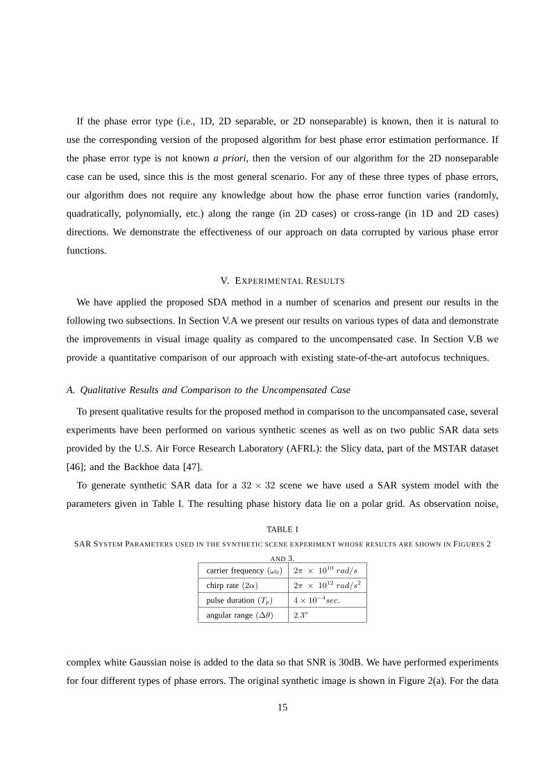
TABLE I

SAR SYSTEM PARAMETERS USED IN THE SYNTHETIC SCENE EXPERIMENT WHOSE RESULTS ARE SHOWN INFIGURES2

AND 3.

carrier frequency(ω0) 2π × 1010 rad/s

chirp rate(2α) 2π × 1012 rad/s2

pulse duration(Tp) 4 × 10−4sec.

angular range(∆θ) 2.3o

complex white Gaussian noise is added to the data so that SNR is30dB. We have performed experiments

for four different types of phase errors. The original synthetic image is shown in Figure 2(a). For the data

15

5 10 15 20 25 30

5

10

15

20

25

30

(a)

5 10 15 20 25 30

5

10

15

20

25

30

(b)

5 10 15 20 25 30

5

10

15

20

25

30

(c)

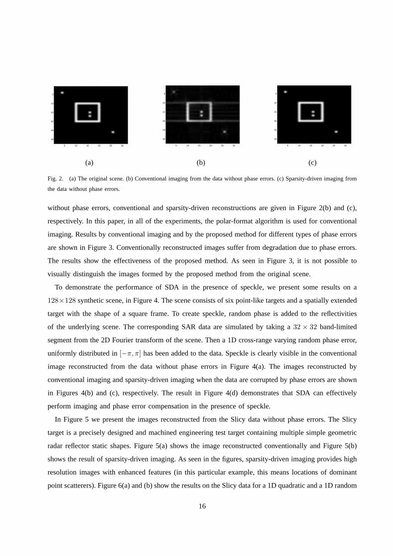
Fig. 2. (a) The original scene. (b) Conventional imaging from the data without phase errors. (c) Sparsity-driven imaging from

the data without phase errors.

without phase errors, conventional and sparsity-driven reconstructions are given in Figure 2(b) and (c),

respectively. In this paper, in all of the experiments, the polar-format algorithm is used for conventional

imaging. Results by conventional imaging and by the proposed method for different types of phase errors

are shown in Figure 3. Conventionally reconstructed images suffer from degradation due to phase errors.

The results show the effectiveness of the proposed method. Asseen in Figure 3, it is not possible to

visually distinguish the images formed by the proposed method from the original scene.

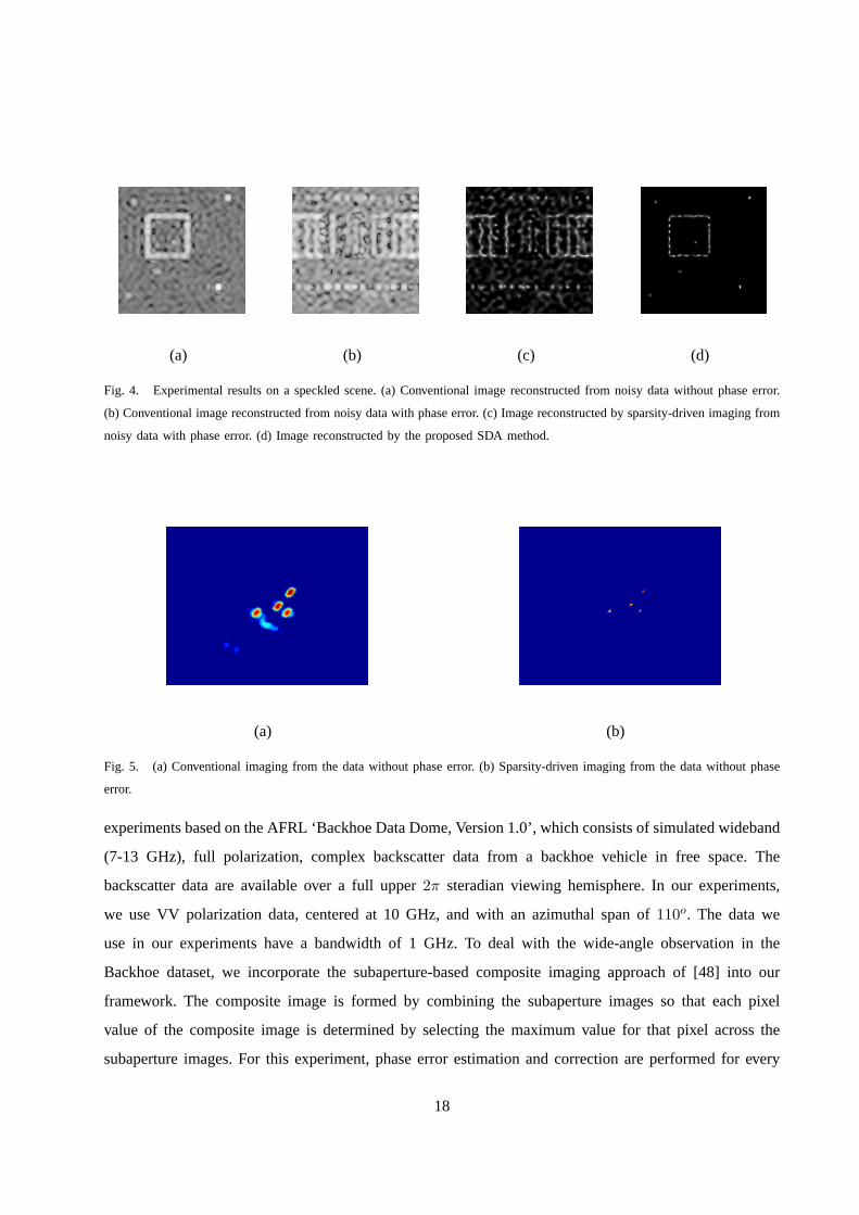
To demonstrate the performance of SDA in the presence of speckle, we present some results on a

128×128 synthetic scene, in Figure 4. The scene consists of six point-like targets and a spatially extended

target with the shape of a square frame. To create speckle, random phase is added to the reflectivities

of the underlying scene. The corresponding SAR data are simulated by taking a32 × 32 band-limited

segment from the 2D Fourier transform of the scene. Then a 1D cross-range varying random phase error,

uniformly distributed in[−π, π] has been added to the data. Speckle is clearly visible in the conventional

image reconstructed from the data without phase errors in Figure 4(a). The images reconstructed by

conventional imaging and sparsity-driven imaging when thedata are corrupted by phase errors are shown

in Figures 4(b) and (c), respectively. The result in Figure 4(d)demonstrates that SDA can effectively

perform imaging and phase error compensation in the presence of speckle.

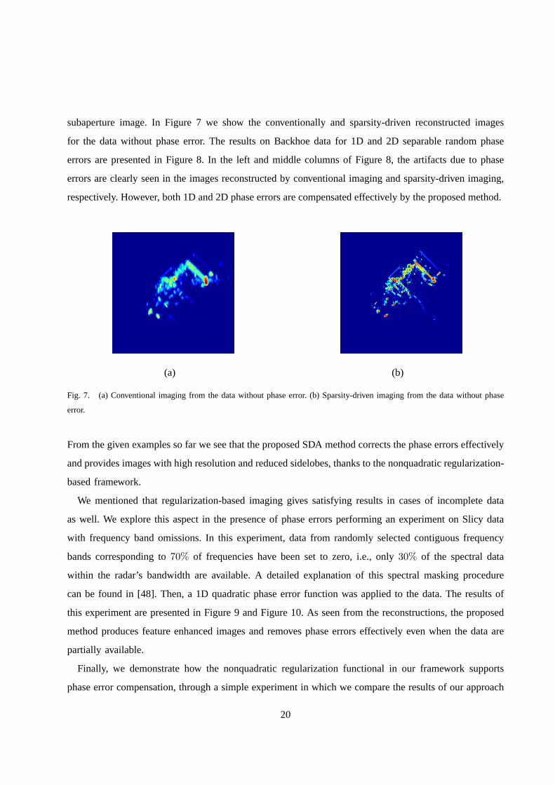
In Figure 5 we present the images reconstructed from the Slicy data without phase errors. The Slicy

target is a precisely designed and machined engineering test target containing multiple simple geometric

radar reflector static shapes. Figure 5(a) shows the image reconstructed conventionally and Figure 5(b)

shows the result of sparsity-driven imaging. As seen in the figures, sparsity-driven imaging provides high

resolution images with enhanced features (in this particular example, this means locations of dominant

point scatterers). Figure 6(a) and (b) show the results on theSlicy data for a 1D quadratic and a 1D random

16

(a)

0 5 10 15 20 25 30 350

2

4

6

8

10

12

Aperture Position

Pha

se E

rror

in r

ad.

5 10 15 20 25 30

5

10

15

20

25

30

5 10 15 20 25 30

5

10

15

20

25

30

(b)

0 5 10 15 20 25 30 35−6

−4

−2

0

2

4

6

Aperture Position

Pha

se E

rror

in r

ad.

5 10 15 20 25 30

5

10

15

20

25

30

5 10 15 20 25 30

5

10

15

20

25

30

(c)

0 5 10 15 20 25 30 35−2

−1.5

−1

−0.5

0

0.5

1

1.5

Aperture Position

Pha

se E

rror

in r

ad.

5 10 15 20 25 30

5

10

15

20

25

30

5 10 15 20 25 30

5

10

15

20

25

30

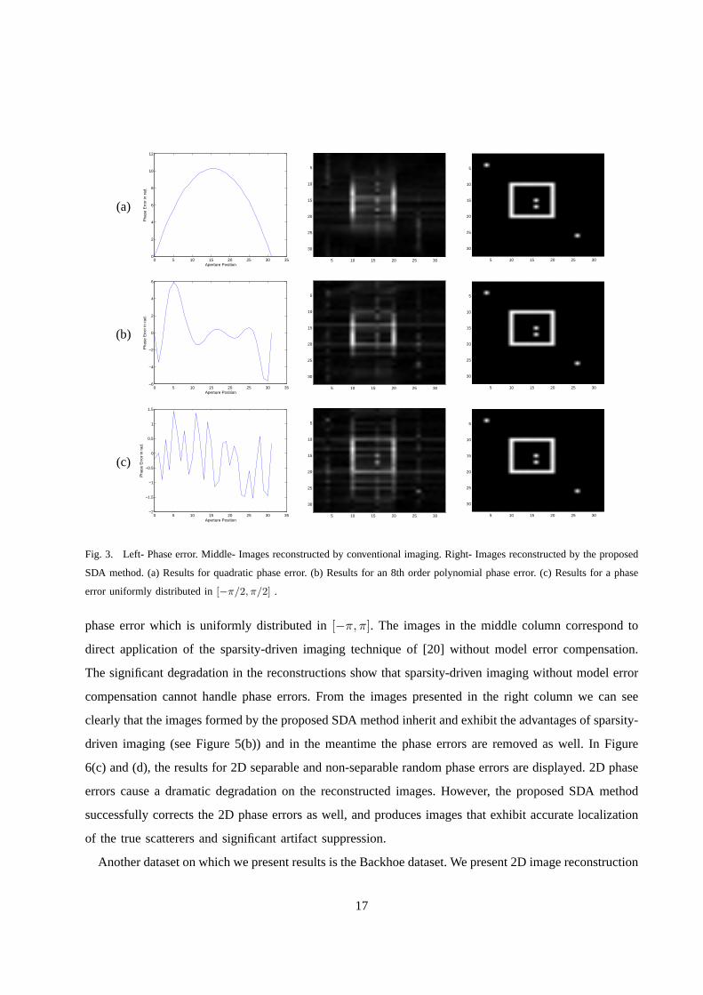
Fig. 3. Left- Phase error. Middle- Images reconstructed by conventional imaging. Right- Images reconstructed by the proposed

SDA method. (a) Results for quadratic phase error. (b) Results for an8th order polynomial phase error. (c) Results for a phase

error uniformly distributed in[−π/2, π/2] .

phase error which is uniformly distributed in[−π, π]. The images in the middle column correspond to

direct application of the sparsity-driven imaging technique of [20] without model error compensation.

The significant degradation in the reconstructions show that sparsity-driven imaging without model error

compensation cannot handle phase errors. From the images presented in the right column we can see

clearly that the images formed by the proposed SDA method inherit and exhibit the advantages of sparsity-

driven imaging (see Figure 5(b)) and in the meantime the phaseerrors are removed as well. In Figure

6(c) and (d), the results for 2D separable and non-separablerandom phase errors are displayed. 2D phase

errors cause a dramatic degradation on the reconstructed images. However, the proposed SDA method

successfully corrects the 2D phase errors as well, and produces images that exhibit accurate localization

of the true scatterers and significant artifact suppression.

Another dataset on which we present results is the Backhoe dataset. We present 2D image reconstruction

17

(a) (b) (c) (d)

Fig. 4. Experimental results on a speckled scene. (a) Conventional image reconstructed from noisy data without phase error.

(b) Conventional image reconstructed from noisy data with phase error. (c) Image reconstructed by sparsity-driven imaging from

noisy data with phase error. (d) Image reconstructed by the proposedSDA method.

(a) (b)

Fig. 5. (a) Conventional imaging from the data without phase error. (b)Sparsity-driven imaging from the data without phase

error.

experiments based on the AFRL ‘Backhoe Data Dome, Version 1.0’, which consists of simulated wideband

(7-13 GHz), full polarization, complex backscatter data from a backhoe vehicle in free space. The

backscatter data are available over a full upper2π steradian viewing hemisphere. In our experiments,

we use VV polarization data, centered at 10 GHz, and with an azimuthal span of110o. The data we

use in our experiments have a bandwidth of 1 GHz. To deal with the wide-angle observation in the

Backhoe dataset, we incorporate the subaperture-based composite imaging approach of [48] into our

framework. The composite image is formed by combining the subaperture images so that each pixel

value of the composite image is determined by selecting the maximum value for that pixel across the

subaperture images. For this experiment, phase error estimation and correction are performed for every

18

(a)

(b)

(c)

(d)

Fig. 6. Left- Images reconstructed by conventional imaging. Middle- Images reconstructed by sparsity-driven imaging. Right-

Images reconstructed by the proposed SDA method. (a) Results for a 1D quadratic phase error. (b) Results for a 1D phase

error uniformly distributed in[−π, π]. (c) Results for a 2D separable phase error composed of two 1D phase errors uniformly

distributed in[−3π/4, 3π/4]. (d) Results for a 2D non-separable phase error uniformly distributedin [−π, π] .

19

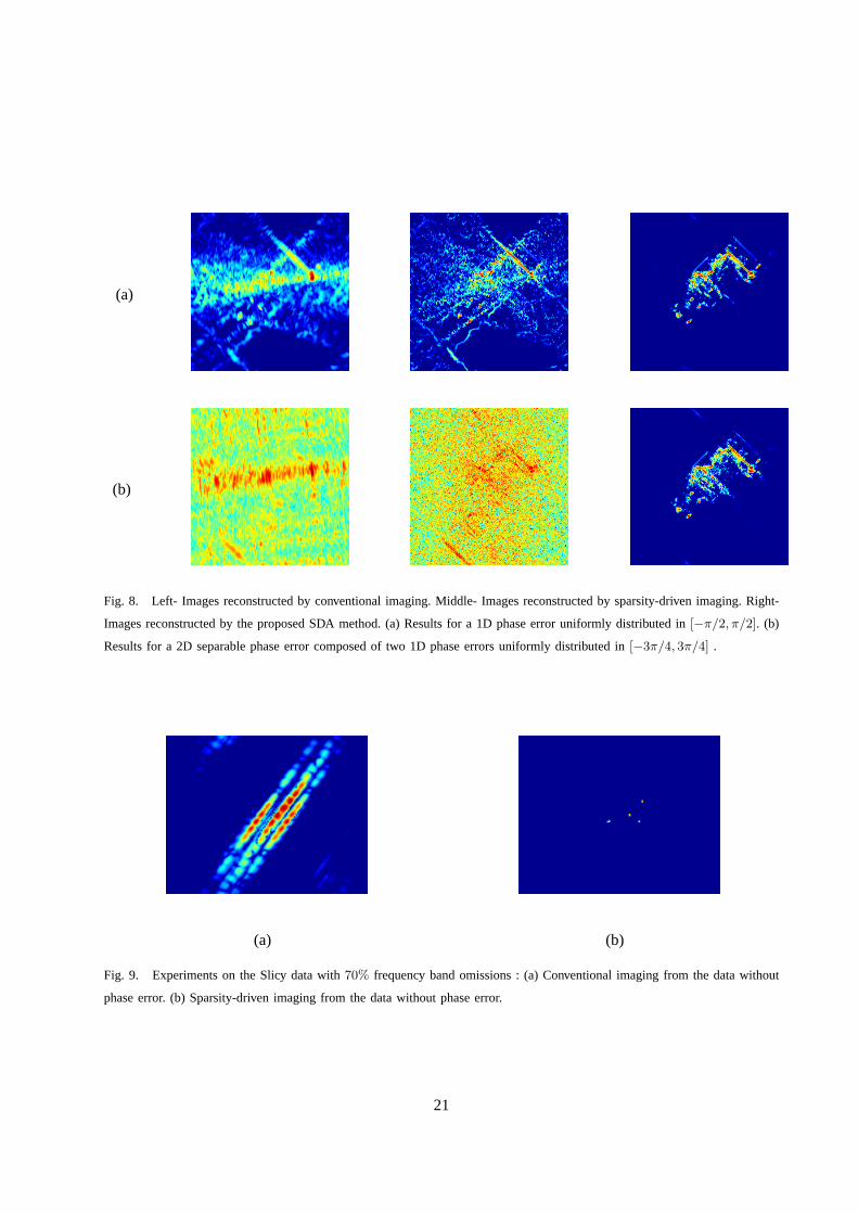
subaperture image. In Figure 7 we show the conventionally andsparsity-driven reconstructed images

for the data without phase error. The results on Backhoe data for 1D and 2D separable random phase

errors are presented in Figure 8. In the left and middle columns of Figure 8, the artifacts due to phase

errors are clearly seen in the images reconstructed by conventional imaging and sparsity-driven imaging,

respectively. However, both 1D and 2D phase errors are compensated effectively by the proposed method.

(a) (b)

Fig. 7. (a) Conventional imaging from the data without phase error. (b)Sparsity-driven imaging from the data without phase

error.

From the given examples so far we see that the proposed SDA method corrects the phase errors effectively

and provides images with high resolution and reduced sidelobes, thanks to the nonquadratic regularization-

based framework.

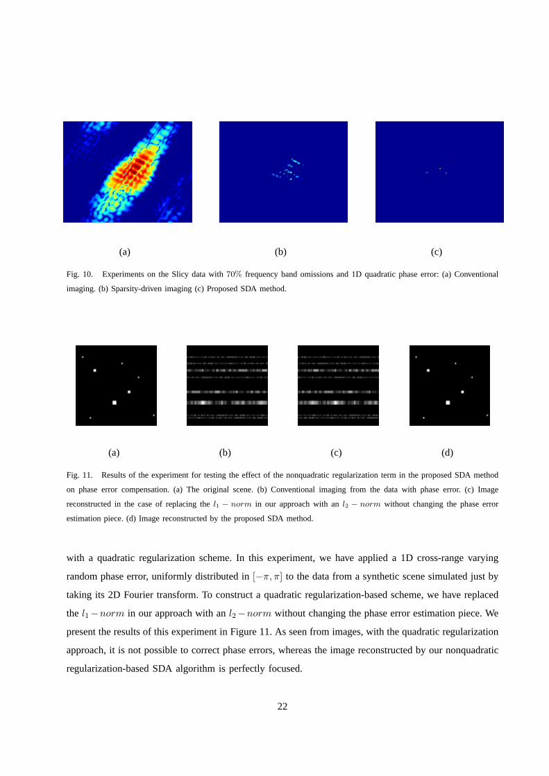
We mentioned that regularization-based imaging gives satisfying results in cases of incomplete data

as well. We explore this aspect in the presence of phase errors performing an experiment on Slicy data

with frequency band omissions. In this experiment, data from randomly selected contiguous frequency

bands corresponding to70% of frequencies have been set to zero, i.e., only30% of the spectral data

within the radar’s bandwidth are available. A detailed explanation of this spectral masking procedure

can be found in [48]. Then, a 1D quadratic phase error functionwas applied to the data. The results of

this experiment are presented in Figure 9 and Figure 10. As seenfrom the reconstructions, the proposed

method produces feature enhanced images and removes phase errors effectively even when the data are

partially available.

Finally, we demonstrate how the nonquadratic regularization functional in our framework supports

phase error compensation, through a simple experiment in which we compare the results of our approach

20

(a)

(b)

Fig. 8. Left- Images reconstructed by conventional imaging. Middle- Images reconstructed by sparsity-driven imaging. Right-

Images reconstructed by the proposed SDA method. (a) Results for a 1D phase error uniformly distributed in[−π/2, π/2]. (b)

Results for a 2D separable phase error composed of two 1D phase errors uniformly distributed in[−3π/4, 3π/4] .

(a) (b)

Fig. 9. Experiments on the Slicy data with70% frequency band omissions : (a) Conventional imaging from the data without

phase error. (b) Sparsity-driven imaging from the data without phaseerror.

21

(a) (b) (c)

Fig. 10. Experiments on the Slicy data with70% frequency band omissions and 1D quadratic phase error: (a) Conventional

imaging. (b) Sparsity-driven imaging (c) Proposed SDA method.

(a) (b) (c) (d)

Fig. 11. Results of the experiment for testing the effect of the nonquadratic regularization term in the proposed SDA method

on phase error compensation. (a) The original scene. (b) Conventional imaging from the data with phase error. (c) Image

reconstructed in the case of replacing thel1 − norm in our approach with anl2 − norm without changing the phase error

estimation piece. (d) Image reconstructed by the proposed SDA method.

with a quadratic regularization scheme. In this experiment, we have applied a 1D cross-range varying

random phase error, uniformly distributed in[−π, π] to the data from a synthetic scene simulated just by

taking its 2D Fourier transform. To construct a quadratic regularization-based scheme, we have replaced

the l1−norm in our approach with anl2−norm without changing the phase error estimation piece. We

present the results of this experiment in Figure 11. As seen from images, with the quadratic regularization

approach, it is not possible to correct phase errors, whereas the image reconstructed by our nonquadratic

regularization-based SDA algorithm is perfectly focused.

22

B. Quantitative Results in Comparison to State-of-the-art Autofocus Methods

In the second part of the experimental study, we present results for comparison of the proposed

technique with existing autofocus techniques. In Figure 12 we show comparative results for a64 × 64

synthetic scene. The SAR data are simulated by taking a band-limited segment on a rectangular grid from

the 2D discrete Fourier transform (DFT) of the scene. Then complex white Gaussian noise is added to

the data so that the input SNR is 10.85dB. Then a 1D cross-range varying random phase error, uniformly

distributed in[−π, π] is added to the data. The performance of the proposed technique is compared to

the performance of PGA [2] and entropy minimization techniques [3, 5–7]. For entropy minimization

we have used the procedure given in [5]. For this particular experiment, the results suggest that all three

methods do a good job in estimating the phase error. However in terms of image quality, while PGA and

entropy minimization are limited by conventional imaging,the proposed SDA method demonstrates the

advantage of joint sparsity-driven imaging and phase errorcorrection, and produces a scene that appears

to provide a very accurate representation of the original scene. For the same synthetic scene we have

also performed experiments with different input SNRs. For each SNR value we have applied 20 different

random 1D phase errors, all of them uniformly distributed in[−π, π]. For each experiment we compute

3 different metrics. These are the MSE between the original image and the image resulting from the

application of the autofocus technique considered, target-to-background ratio, and metrics for the phase

error estimation error. These metrics are computed as follows:

MSE =1

I

∥∥∥|f | −

∣∣∣f

∥∥∥

∣∣∣

2

2(43)

Here,f and f denote the original and the reconstructed images, respectively. I is the total number of

pixels.

Target-to-background ratio is used to determine the accentuation of the target pixels with respect to

the background:

TBR = 20 log10

maxi∈T

∣∣∣fi

∣∣∣

1IB

∑

j∈B

∣∣∣fj

∣∣∣

(44)

Here,T andB denote the pixel indices for the target and the background regions, respectively.IB is the

number of background pixels.

To compare the phase error estimation performance of the proposed method to other techniques, we

first compute the estimation error for phase errors:

φe = φ − φ (45)

23

(a) (b) (c)

(d) (e) (f)

Fig. 12. (a) The original scene. (b) Conventional imaging from noisy data without phase error. (c) Conventional imaging from

noisy data with phase error. (d) Result of PGA. (e) Result of entropy minimization. (f) Result of the proposed SDA method.

Hereφe is effectively the phase error that remains in the problem after correction of the data or the model

using the estimated phase error. To evaluate various techniques based on their phase error estimation

performance, it makes sense to first remove the components inφe that either have no effect on the

reconstructed image, or that can be easily dealt with, and then perform the evaluation based on the

remaining error. We first note that a constant (as a function ofthe aperture position) phase shift has no

effect on the reconstructed image [1]. Second, a linear phaseshift does not cause blurring, but rather a

spatial shift in the reconstructed image. Such a phase error can be compensated by appropriate spatial

operations on the scene [4], which we perform prior to quantitative evaluation. To disregard the effect of

any constant phase shift in our evaluation, and also noting that the amount of variation of the phase error

across the aperture is closely related to the degree of degradation of the formed imagery, we propose

using evaluation metrics based on the total variation (TV) ofφe and on thel2 − norm of the gradient

24

of φe:

TVPE =1

M − 1‖∇φe‖1 (46)

MSEPE =1

M − 1‖∇φe‖

22

Here, ∇φe is the (M − 1) × 1 vector, obtained by taking first-order differences between successive

elements ofφe. M is the total number of cross-range positions.

Now we get back to the quantitative evaluation of the reconstruction of the scene in Figure 12(a)

for various SNRs. We present the comparison results for thesethree metrics in Figure 13. SinceTVPE

and MSEPE values are similar for these particular experiments, for the sake of space we show the

results forMSEPE only. From the plots presented, it is clearly seen that the proposed method performs

better than the other techniques, especially for low SNR values. We also note in Figure 13(a) that the

proposed SDA method yields much better performance in terms of the MSE between the original and the

reconstructed images even at high SNRs. This is due to the fact that SDA benefits from the advantages

of sparsity-driven imaging (unlike the other techniques) over conventional imaging (see Figure 12) in

addition to successfully correcting the phase errors (likethe other techniques) at high SNRs.

All of the three algorithms were implemented using non-optimized MATLAB code on an Intel Celeron

2.13GHz CPU. In the experiment of Figure 12, the computation times required by PGA, entropy minimiza-

tion, and the proposed SDA method are 0.6240s, 1.1076s, and 2.1216s, respectively. For the experiments of

Figure 13, the average computation times for PGA, entropy minimization, and SDA are 0.3095s, 0.4719s,

and 3.4961s, respectively. The computational load of SDA is relatively more than the other methods, but

this can be justified through the benefits provided by the sparsity-driven imaging framework underlying

SDA, as demonstrated in our experiments.

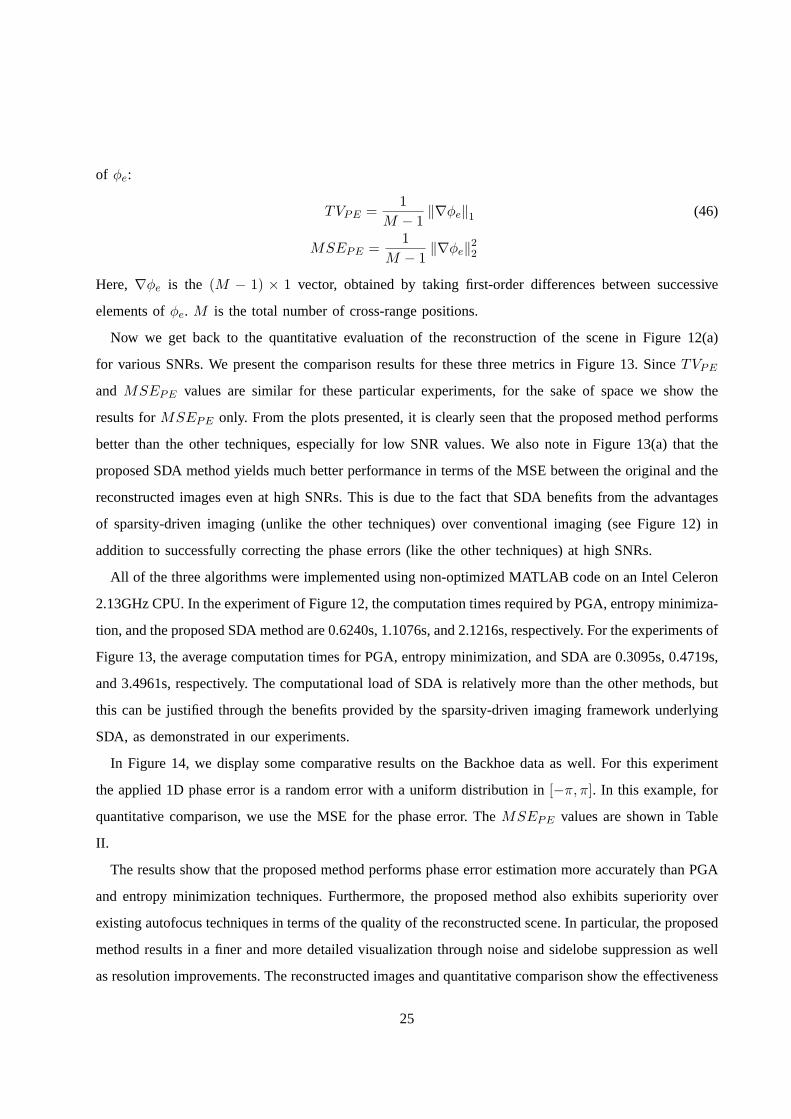
In Figure 14, we display some comparative results on the Backhoe data as well. For this experiment

the applied 1D phase error is a random error with a uniform distribution in [−π, π]. In this example, for

quantitative comparison, we use the MSE for the phase error. The MSEPE values are shown in Table

II.

The results show that the proposed method performs phase error estimation more accurately than PGA

and entropy minimization techniques. Furthermore, the proposed method also exhibits superiority over

existing autofocus techniques in terms of the quality of thereconstructed scene. In particular, the proposed

method results in a finer and more detailed visualization through noise and sidelobe suppression as well

as resolution improvements. The reconstructed images and quantitative comparison show the effectiveness

25

−8 −6 −4 −2 0 2 4 6 8 10 120

0.005

0.01

0.015

0.02

0.025

Input SNR in dB

MS

E

PGAEntropy Min.Proposed

(a)

−8 −6 −4 −2 0 2 4 6 8 10 1215

20

25

30

35

40

45

50

55

60

65

Input SNR in dB

Tar

get−

to−

back

grou

nd R

atio

PGAEntropy Min.Proposed

(b)

−8 −6 −4 −2 0 2 4 6 8 10 120

0.1

0.2

0.3

0.4

0.5

0.6

0.7

Input SNR in dB

MS

E fo

r P

hase

Err

or

PGAEntropy Min.Proposed

(c)

Fig. 13. Quantitative evaluation of the reconstruction of the scene in Figure12(a) for various SNRs. Each point on the curves

corresponds to an average over 20 experiments with different random 1D phase errors uniformly distributed in[−π, π]. (a) MSE

versus SNR. (b) Target-to-background ratio versus SNR. (c) MSE for phase error estimations versus SNR.

of the proposed approach.

Finally, we compare our method with the recently proposed multichannel autofocus (MCA) technique

[12]. We have generated a64 × 64 synthetic scene that satisfies the requirements of MCA, involving

a condition on the rank of the image, as well as the presence ofa low-return region in the scene.

The SAR data used in these experiments are corrupted by a 1D cross-range varying random phase

error, uniformly distributed in[−π, π]. We show the results of the experiments performed for various

input SNR levels in Figure 15. We observe that both MCA and SDA perform successful phase error

compensation at the relatively high SNR of 27 dB (see Figure 15(c) and (d)). However when SNR is

reduced to 10 dB, MCA is not able to correct the phase error, asshown in Figure 15(f). On the other

hand, SDA compensates phase errors, and suppresses noise andclutter effectively even for this relatively

low SNR case, as shown in Figure 15(g). Figure 15(h) contains a plot of MSEs for phase error estimation

achieved by MCA and SDA on this scene for various SNR levels. Thisplot demonstrates the robustness

of SDA to noise. Average computation times required by MCA andthe proposed SDA method for the

experiments displayed in Figure 15 are 0.1629s and 2.5151s, respectively (using non-optimized MATLAB

code on an Intel Celeron 2.13GHz CPU). The results of these experiments show that although MCA is

a fast algorithm, working very well in scenarios involving high-quality data, its performance degrades

significantly as SNR decreases.

26

(a) (b) (c)

(d) (e) (f)

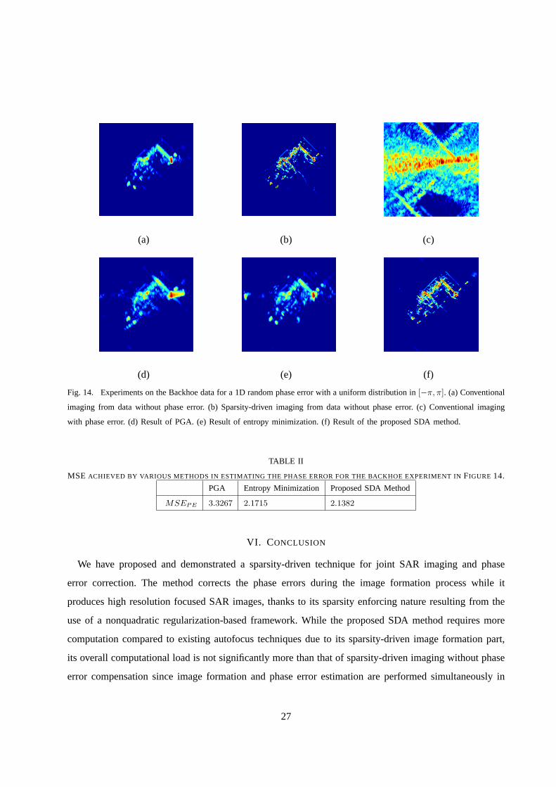
Fig. 14. Experiments on the Backhoe data for a 1D random phase errorwith a uniform distribution in[−π, π]. (a) Conventional

imaging from data without phase error. (b) Sparsity-driven imaging from data without phase error. (c) Conventional imaging

with phase error. (d) Result of PGA. (e) Result of entropy minimization.(f) Result of the proposed SDA method.

TABLE II

MSE ACHIEVED BY VARIOUS METHODS IN ESTIMATING THE PHASE ERROR FOR THE BACKHOE EXPERIMENT INFIGURE 14.

PGA Entropy Minimization Proposed SDA Method

MSEPE 3.3267 2.1715 2.1382

VI. CONCLUSION

We have proposed and demonstrated a sparsity-driven technique for joint SAR imaging and phase

error correction. The method corrects the phase errors during the image formation process while it

produces high resolution focused SAR images, thanks to its sparsity enforcing nature resulting from the

use of a nonquadratic regularization-based framework. While the proposed SDA method requires more

computation compared to existing autofocus techniques dueto its sparsity-driven image formation part,

its overall computational load is not significantly more thanthat of sparsity-driven imaging without phase

error compensation since image formation and phase error estimation are performed simultaneously in

27

(a) (b) (c) (d)

(e) (f) (g)

10 15 20 25 300

0.2

0.4

0.6

0.8

1

1.2

1.4

1.6

1.8

Input SNR in dB

MS

E fo

r P

hase

Err

or

MCAProposed

(h)

Fig. 15. (a) The original scene. (b) Conventional imaging from noisy phase-corrupted data for input SNR of27dB. (c) Result

of MCA for input SNR of 27dB. (d) Result of the proposed SDA method for input SNR of27dB. (e) Conventional imaging

from noisy phase-corrupted data for input SNR of10dB. (f) Result of MCA for input SNR of10dB. (g) Result of the proposed

SDA method for input SNR of10dB. (h) MSEs for phase error estimation versus SNR.

the proposed method. The method can handle 1D as well as 2D phase errors. Experimental results on

various scenarios demonstrate the effectiveness of the proposed approach as well as the improvements it

provides over existing methods for phase error correction.

In this work we considered SAR, but our approach is applicablein other areas, where similar types

of model errors are encountered, as well. Since the proposed method has a sparsity-driven structure, it is

applicable only to radar imaging scenarios in which the underlying scene admits a sparse representation

in a particular domain. Other potential extensions may be the formulation of the problem for scenarios

involving sparse representations of the field in various spatial dictionaries or incorporation of prior

information or some constraints on phase error. For future work, model errors in multistatic scenarios

and target motion induced phase errors would be of interest as well.

28

APPENDIX

In this appendix, we describe how we get from Eqn. (28) to Eqn. (29). The cost function in (28) for

phase error estimation is as follows:

φ(n+1)1D (m) = arg min

φ1D(m)J(f (n+1), φ1D(m)) = arg min

φ1D(m)

∥∥∥gm − e(jφ1D(m))Cmf (n+1)

∥∥∥

2

2

for m = 1, 2, ...., M

Here, M denotes the total number of cross-range positions. When we evaluate the norm expression we

get∥∥∥gm − e(jφ1D(m)) Cmf (n+1)

∥∥∥

2

2= (gm − e(jφ1D(m)) Cmf (n+1))H (gm − e(jφ1D(m)) Cmf (n+1))

= gHm gm − gH

me(jφ1D(m))Cmf (n+1) − f (n+1)H

CHm

(

e(jφ1D(m)))H

gm + f (n+1)H

CHm

(

e(jφ1D(m)))H

︸ ︷︷ ︸

e(−jφ1D(m))

e(jφ1D(m))Cmf (n+1)

= gHm gm − gH

m[cos(φ1D(m)) + j sin(φ1D(m))]Cmf (n+1) − f (n+1)H

CHm [cos(φ1D(m)) − j sin(φ1D(m))]gm + f (n+1)H

CHm Cmf (n+1)

= gHm gm − 2Re{cos(φ1D(m))f (n+1)H

CHm gm} + 2Re{j sin(φ1D(m))f (n+1)H

CHm gm} + f (n+1)H

CHm Cmf (n+1)

= gHm gm − 2 cos(φ1D(m))Re{f (n+1)H

CHm gm} − 2 sin(φ1D(m))Im{f (n+1)H

CHm gm} + f (n+1)H

CHm Cmf (n+1)

Let Re{f (n+1)H

CHm gm} = < andIm{f (n+1)H

CHm gm} = =

Since we can writesin(φ1D(m)) ascos(φ1D(m) − π2 ) the equation becomes

∥∥∥gm − ejφ1D(m)Cmf (n+1)

∥∥∥

2

2= gH

m gm − 2[< cos(φ1D(m)) + = cos(φ1D(m) −π

2)] + f (n+1)H

CHm Cmf (n+1)

The cosines in the previous equation can be added with phasor addition rule to a single cosine. The

phasors for the terms< cos(φ1D(m)) and= cos(φ1D(m) − π2 ) can be seen below.

P1 = Rej0 = < P2 = =e−jπ

2 = −j=

If we add the phasors

P1 + P2 = < + (−j=) = <− j=

we can find the magnitude and the phase of the new cosine as

magnitude =√

<2 + =2 phase = arctan(−=

<)

Finally, we can write∥∥∥gm − ejφ1D(m) Cmf (n+1)

∥∥∥

2

2= gH

m gm − 2√

<2 + =2 cos[φ1D(m) + arctan(−=

<)] + f (n+1)H

CHm Cmf (n+1)

29

REFERENCES

[1] C. V. Jakowatz, Jr., D. E. Wahl, P. H. Eichel, D. C. Ghiglia, and P. A. Thompson,Spotlight-Mode

Synthetic Aperture Radar: A Signal Processing Approach, Springer, 1996.

[2] D. E. Wahl, P. H. Eichel, D. C. Ghiglia, and C. V. Jakowatz, Jr., “Phase Gradient Autofocus - A

robust tool for high resolution SAR phase correction,”IEEE Trans. Aerosp. Electron.Syst., vol. 30,

no. 7, pp. 827–835, 1994.

[3] L. Xi, L. Guosui, and J. Ni, “Autofocusing of ISAR images based on entropy minimization,”IEEE

Trans. Aerosp. Electron. Syst., vol. 35, no. 10, pp. 1240–1252, 1999.

[4] J. R. Fienup, “Synthetic-aperture radar autofocus by maximizing sharpness,”Optics Letters, vol.

25, pp. 221–223, 2000.

[5] J. R. Fienup and J. J. Miller, “Aberration correction by maximizing generalized sharpness metrics,”

J. Opt. Soc. Amer. A, vol. 20, no. 4, pp. 609–620, 2003.

[6] T. J. Kragh, “Monotonic iterative algorithm for minimum-entropy autofocus,”Adaptative Sensor

Array Processing (ASAP), 2006.

[7] R. L. Morrison, Jr., M. N. Do, and D. C. Munson, Jr., “SAR image autofocus by sharpness

optimization: A theoretical study,”IEEE Trans. Image Processing, vol. 16, pp. 2309–2321, 2007.

[8] F. Berizzi and G. Corsini, “Autofocusing of inverse synthetic aperture radar images using contrast

optimization,” IEEE Trans. Aerosp. Electron. Syst., vol. 32, no. 7, pp. 1185–1191, 1996.

[9] M. P. Hayes and S. A. Fortune, “Recursive phase estimationfor image sharpening,”presented at

the Image and Vision Computing New Zealand, 2005.

[10] R. G. Paxman and J. C. Marron, “Aberration correction ofspeckled imagery with an image-sharpness

criterion,” Statistical Optics, Proc. SPIE, vol. 976, pp. 37–47, 1988.

[11] T. C. Calloway and G. Donohoe, “Subaperture autofocus for synthetic aperture radar,”IEEE Trans.

Aerosp. Electron. Syst., vol. 30, pp. 617–621, 1994.

[12] R. L. Morrison, Jr., M. N. Do, and D. C. Munson, Jr., “MCA: Amultichannel approach to SAR

autofocus,”IEEE Trans. Image Processing, vol. 18, pp. 840–853, 2009.

[13] W. D. Brown and D. C. Ghiglia, “Some methods for reducing propagation-induced phase errors in

coherent imaging systemsI: Formalism,”J. Opt. Soc. Amer. A, vol. 5, pp. 924–942, 1988.

[14] D. C. Ghiglia and W. D. Brown, “Some methods for reducing propagation-induced phase errors in

coherent imaging systemsII: Numerical results,”J. Opt. Soc. Amer. A, vol. 5, pp. 943–957, 1988.

[15] C. V. Jakowatz, Jr., and D. C. Ghiglia, “Eigenvector method for maximum-likelihood estimation

30

of phase errors in synthetic aperture radar imagery,”J. Opt. Soc. Amer. A, vol. 10, pp. 2539–2546,

1993.

[16] P. H. Eichel, D. C. Ghiglia, and C. V. Jakowatz, Jr., “Speckle processing method for synthetic

aperture radar phase correction,”Opt. lett., vol. 14, pp. 1101–1103, 1989.

[17] L. Kuang-Hung, A. Wiesel, and D. C. Munson, Jr., “Synthetic aperture radar autofocus via

semidefinite relaxation,”IEEE Int. Conf. Acoustics, Speech, Signal Processing, 2010.

[18] W. G. Carrara, R. M. Majewski, and R. S. Goodman,Spotlight Synthetic Aperture Radar: Signal

Processing Algorithms, Artech House, 1995.

[19] J. Walker, “Range-doppler imaging of rotating objects,” IEEE Trans. Aerosp. Electron. Syst, vol.

AES-16, pp. 23–52, 1980.

[20] M. Cetin and W.C. Karl, “Feature-enhanced synthetic aperture radar image formation based on

nonquadratic regularization,”IEEE Trans. Image Processing, pp. 623–631, 2001.

[21] J. W. Burns, N. S. Subotic, and D. Pandelis, “Adaptive decomposition in electromagnetics,”in

Proc. Int. Symp. Antennas Propag. Soc., pp. 1984–1987, 1997.

[22] T. J. Kragh and A. A. Kharbouch, “Monotonic iterative algorithms for sar image restoration,”in

Proc. IEEE Int. Conf. Image Processing, pp. 645–648, 2006.

[23] A. C. Kak and M. Slaney,Principles of Computerized Tomographic Imaging, New York: IEEE

Press, 1988.

[24] D. C. Munson, Jr., J. D. O’Brien, and W. K. Jenkins, “A tomographic formulation of spotlight-mode

synthetic aperture radar,”Proc. IEEE, vol. PROC-71, pp. 917–925, 1983.

[25] D. W. Warner, D. Ghiglia, A. FitzGerrell, and J. Beaver, “Two-dimensional phase gradient

autofocus,”Image reconstruction from incomplete data, Proc. SPIE, vol. 4123, pp. 162–173, 2000.

[26] D. L. Donoho and M. Elad, “Optimally sparse representation in general (non-orthogonal) dictionaries

via l1 minimization,” Proc. Natl. Acad. Sci., vol. 100, pp. 2197–2202, 2003.

[27] L. C. Potter, E. Ertin, J. T. Parker, and M. Cetin, “Sparsity and compressed sensing in radar imaging,”

Proc. of the IEEE, vol. 98, pp. 1006–1020, 2010.

[28] V. M. Patel, G. R. Easley, D. M. Healy, and R. Chellappa, “Compressed synthetic aperture radar,”

IEEE Journal of Selected Topics in Signal Processing, vol. 4, pp. 244–254, 2010.

[29] R. Baraniuk and P. Steeghs, “Compressive radar imaging,” in Proc. IEEE 2007 Radar Conf., pp.

128–133, 2007.

[30] C. Gurbuz, J. McClellan, and R. Scott, Jr., “A compressive sensing data acquisition and imaging

31

method for stepped frequency GPRs,”IEEE Trans. Signal Processing, vol. 57, pp. 2640–2650,

2009.

[31] I. Stojanovic, W. C. Karl, and M. Cetin, “Compressed sensing of mono-static and multi-static SAR,”

Algorithms Synthetic Aperture Radar Imagery XVI, Proc. SPIE, 2009.

[32] C. Berger, S. Zhou, and P. Willett, “Signal extraction using compressed sensing for passive radar

with OFDM signals,” in Proc. 11th Int. Conf. Inf. Fusion, p. 16, 2008.

[33] I. Stojanovic and W.C. Karl, “Imaging of moving targets with multi-static SAR using an

overcomplete dictionary,”IEEE Journal of Selected Topics in Signal Processing, vol. 4, pp. 164–176,

2010.

[34] M. Cetin and A. Lanterman, “Region-enhanced passive radar imaging,” Proc. Inst. Elect. Eng.

Radar, Sonar Navig., vol. 152, pp. 185–194, 2005.

[35] M. A. Herman and T. Strohmer, “High-resolution radar viacompressed sensing,”IEEE Trans.

Signal Processing, vol. 57, pp. 2275–2284, 2009.

[36] K. R. Varshney, M. Cetin, J. W. Fisher, III, and A. S. Willsky, “Sparse signal representation in

structured dictionaries with application to synthetic aperture radar,”IEEE Trans. Signal Processing,

vol. 56, pp. 3548–3561, 2008.

[37] C. D. Austin and R. L. Moses, “Wide-angle sparse 3D synthetic aperture radar imaging for nonlinear

flight paths,” in Proc. IEEE Nat. Aerosp. Electron. Conf., pp. 330–336, 2008.

[38] C. Austin, E. Ertin, and R. L. Moses, “Sparse multipass 3D imaging: Applications to the GOTCHA

data set,”Defense Security Symp. Algorithms Synthetic Aperture Radar Imagery XVI, Proc. SPIE,

vol. 7337, pp. 733703–1733703–12, 2009.

[39] M. Ferrara, J. Jackson, and M. Stuff, “Three-dimensional sparse-aperture moving-target imaging,”

Algorithms Synthetic Aperture Radar Imagery XIV, Proc. SPIE, vol. 6970, 2008.

[40] D. L. Mensa,High Resolution Radar Imaging, MA: Artech House, 1981.

[41] B. Borden, “Maximum entropy regularization in inversesynthetic aperture radar imagery,”IEEE

Trans. Signal Processing, vol. 40, pp. 969–973, 1992.

[42] M. Herman and T. Strohmer, “General deviants: An analysis of perturbations in compressed sensing,”

IEEE Journal of Selected Topics in Signal Processing: Special Issue on Compressive Sensing, vol.

4(2), pp. 342–349, 2010.

[43] M. Cetin, W. C. Karl, and A. S. Willsky, “Feature-preserving regularization method for complex-

valued inverse problems with application to coherent imaging,” Opt. Eng., vol. 45, 2006.

32

[44] N. O. Onhon and M. Cetin, “A nonquadratic regularization based technique for joint SAR imaging

and model error correction,”Algorithms for Synthetic Aperture Radar Imagery XVI, Proc. SPIE,

vol. 7337, 2009.

[45] N. O. Onhon and M. Cetin, “Joint sparsity-driven inversion and model error correction for radar

imaging,” IEEE Int. Conf. Acoustics, Speech, Signal Processing, pp. 1206–1209, 2010.

[46] MSTAR, Air Force Research Laboratory, Model Based Vision Laboratory, Sensor Data Management

System, http://www.mbvlab.wpafb.af.mil/public/sdms/datasets/mstar/.

[47] Backhoe Data Sample & Visual-D Challenge Problem, Air Force Research Laboratory, Sensor Data

Management System, https://www.sdms.afrl.af.mil/main.htm.

[48] M. Cetin and R. L. Moses, “SAR imaging from partial-aperture data with frequency-band omissions,”

Algorithms for Synthetic Aperture Radar Imagery XII, Proc. SPIE, vol. 5808, pp. 32–43, 2005.

33