■ ■ ■ ' ' ■ ■' —

AD-778 458

NEAR-FIELD OBSERVATIONS AND SOURCE PARAMETERS OF CENTRAL CALIFORNIA EARTHQUAKES

Lane R. Johnson, et al

California University

Prepared for:

Air Force Office of Scientific Research

December 1973

••

N

DISTRIBUTED BY:

KIT] National Technicrl Information Service U. S. DEPARTMENT OF COMMERCE 5285 Port Royal Road, Springfield Va. 72151

_UKCLASSIFIED v-runtv Ci.i«'.ifir,i'. in AD- 77^ g£g

DOCUMENT CONTROL DATA- R&D ' -r»u,/,y f,.,.,„<.„oo c/ ,„.■>. ^ ./ g^ugc. gg .^ , .„. „„^ r,us, „ cn,.ff,, ,„.,(,,^,

I- OM.&,^»7iNC »CTlViTV lCor-t,0rml» »uit.or} Tt '. • 1 _• ... en lie • nil ♦•• "£ "O" T SC C u Hi T Y c L» i»l Fl C » T1CN miversity of Cjliforni.3, Berkeley Geology and Geophysics

; Berkeley, CA 94720 » «ewowr TITLE

UNCLASSIFIED ib. CROUP

KEAH-FISLD OBSERVATIONS AND S01P.CE PARAMETERS OF CEOTRAL CALIFORIIIA EARTHQUAKES

■• CEiCB-^nve NOTES (TVp» ot rcpon »nd ,nclu,,v dmlct)

Scientific. »• »u --oai», fFint •• mm-, miaalm inutal, Imtt nmmm)

Lane R. Johnson and Thomas V. McEvlUy

»• REPsn T DATE

December, 1973 •». CONTRACT OK OB«NT NO

AFOSR-72-2392 ft. »BOJEC T NO.

AO 1827-7

62701E

»•• TOTAU NO. OF PASES

66 76. NO. OF RCFS

»A. ORICiNATCn-S REPORT NUMBER(S|

IC. CISTRieuTION STATEMENT

IOTP-TR -74.-0635

Approved for public release; distribution unlimited.

^UPPUEMENTARV NOTES

TECH, OTHER

fJATIONAL TECHNICAI INr0RMATI0N SFRVICE '■ ^ P«P«r»nwit of Conmert»

Spiirj"

• i r»~ AC T

12. SPONSORING MILITARY ACTIVITY

AR Office of Scientific Research/NP .400 Wilson Boulevard Arlington, VA Arlington, VA 22209

^is p a study of source characteristics of 13 earthquakes with magnitudes between 2.4 and 5.1 located near the San Andreas fault in central California On the oasis of nypocentral locations and fault plane solution« the earthquakes separate into two source groups, one group clearly related to the throughgoing nortnwest trending San Andreas fault zone and the other apparently associated with generally north trending bifurcations such as the Calaveras fault. The basic data consist of broadband recordings (0.03 to 10 Hz) of theM earthquakes at two sites of the San Andreas Geophysical 0bser\atory (SAGO). Epicentral distances range between 2 and 4o km, and maximum ground displacements from 4 to 4000 microns were recorded. Tr.e whole-record spectra computed from the seismograms lend themselves to source parameter studies in that they can be interpreted in terms of low-frequency level, corner frequency, and higv--frequency slope. The influence of tilts and nonlinear response of the seismometer was considered in the interpretation of the low frequencies. Seismic source moments estimated fron the low-frequency levels of the spectra show a linear dependence upon magnitude with a slope slightly greater than 1. The geology at the recording site can contribute an uncertainty factor of at least 3 to the estimated moments. Synthetic seismograms have also been used to estimate seismic moments in both the time domain and frequency domain, and the results compare favorably with t^nsp estimated directly frc"" ^h0 Ic»r-f*aauencv IAVBIA nf «!#■ ,«~*..- «■,„, , corner frequencies are onl> weakly dependent upon magnitude. Interpreted in therms of source dimension, these corner frequercies Imply values of 1 to 2 km for the earthquakes of this study. The corner frequencies may also be interpreted

JU .Noy0!l<4 /O (abstract continued on reverse) UNCLASSIFIED

■

\

__

wmm wm - mm

Sircunly n.is^ifu ntion I,

// I 4

HKV WOROI

eartb.qoakes • ■ source parameters central California San Andreas fault seismic spectra seismic moments . earthquake source models near field

(abstract continued)

in terms of the rise time of the source function, yifelding 0.5 to 1.0 sec. The data indicate that the earthquakes of surprisingly similar in their source parameters, iritjj only showing a strong dependence on magnitude.

value this the s

in t tudy ;ismic

le ran ire al. momen

ce

ria*>in«a

-

11

ABSTRACT

This is a study of source characteristics of 13 earthquakes with magnitudes

between 2.1» and 5.1 located near the San Andreas fault in central California.

On the basis of hypocentml locations and fault plane solutions the earthquakes

separate into two source groups, one group clearly related to the throughgoing

northwest trending San Andreas fault zone and the other apparently associated

with generally north trending bifurcations such as the Calaveras fault. T*

basic data consist of broadband recordings (0.05 to 10 Hz) of these earthquakes

at two sites of the San Andreas Geophysical Observatory (SAGO). Epicentral

distaices range between 2 and kO km, and maximum ground displacements from k

to '4000 microns were recorded. The whole-record spectra computed from the

seismograms lend themselves to source parameter studies in that they can be

interpreted in terms of low-frequency lev^l, corner frequency, and higl:-frequency

slope. The influence cf tilts and nonlinear response of the seismometer was

considered in the interpretation of the low frequencies. Seismic source moments

estimated from the low-frequency levels of the spectra show a linear dependence

upon magnitude with P. slope slightly greater than 1. The geology at the recording

site can contribute an uncertainty factor of at least 5 to the estimated moments.

Synthetic seismograms have also been used to estimate seismic moments in both

the time domain and frequency domain, and the results compare favorably with

those estimated directly from the low-frequency levels of the spectra. Observed

corner frequencies are only weakly dependent upon magnitude. Interpreted in

terms of source dimension, these -orner frequencies imply values of 1 to 2 km

for the earthquakes of this study. The corner frequencies may also be interpreted

in terms of the rise time of the source function, yielding values in the range

0.5 to 1.0 sec. The data indicate that the earthquakes of this study are all

surpriRingly bimiler in their source parameters, wUh only the seismic moment

showing a strong dependence on magnitude.

--

INTRODUCTION

In 1966-67 the San Andreas Geophysical Observatory (SAGO) was established

on the San Andreas fault zone in central Calirornia some 5 miles south of

Hollister. The primary purpose of the observatory is the long-term study

of various geophysical phenomena associated with an active se©nent of the

fault zone. A variety of seismometers recording on mapretic tape monitor

local earthquakes In the magnitude range from microearthquakes ot VL = -1

and less up through strong local shocks of M. = 5 or more with displacements

of several mm. Tim seismometers plus tilt and strain meters, magnetometers,

telluric current monitors, and others are distributed along the fault zone

in a region about 5 km square.

SAGO is located between two rlusters of earthquake activity which form

the main concentrations of ongoing moderate seismicity in central California.

Within 50 km along the San Andreas fault zone to the southeast of SAGO lies

the seismically active St^ne Canyon and Bear "alley region, while the same

distance to the northwest includes the cluster0 of seismicity near San Juan

Bautista and Corralitos. In this 100 km length along the Sar. Andreas fault

zone, centered at SAGO and including the bifurcation with the Calaveras fault,

occur most central California earthquakes (Bolt et al., 1968; Bolt and Miller,

1971), with an average over recent years of about one event per year with M^

greater than '^.5. Earthquake mechanisms are generally of right-lateral,

transcurrent type. Fault slippage through creep is observed on both the San

Andreas and Calaveras fault traces in the region, with average slip rates

exceeding 1 cm/yr at scxnt localitief. This area is undoubtedly one of the

most heavily instrumentcc. and thoroughly studied xegions of earthquake activity

in the world.

—'

This study is an investigation of near-field radiation from locel

earthquakes recorded on broadband seismcmeter systems at SAGO. From the

library of events preserved on magnetic tape, 13 earthquakes were selected

with a magnitude range of 2.h to 5.1, an epicentral distance range of 2 to

ko km, and a variety of apparent source geometrj.es relative to the main

throughgoing San Andreas fault trace. The data set samples a range of

magnitudes at a given distance for one type of comparison and a range of

distances at a given magnitude for another.

Motivation for near-field studies comes from several areas. By making

observations with broadband instrumentation within a few source depths,

source dimensions, or wavelengths one would hope to obtain better definition

of the detailed structure in the radiated waves and consequently improve

the ability to make inferences on a specific earthquake source model. In

addition to the scientific gain in increased knowledge of the source,

differentiation among alternative models with subtle variations In radiated

waves is important in understanding the basis for observed discriminants

between earthquakes and explosions. Finally, specification of a working

model fhr the dynamics of an earthquake source can lead to direct computation

of strong motion in the near-field of potentially damaging earthquakes, and

thus provide additional capability in determining design earthquake motions

in earthquake engineering practice.

w .......

DATA

Figure 1 shows the 2 SAGO seismographic stations and 1? earthquakes

involv.'d in thid study. The SAGO-Central station (SAO) is 2 km southwest

of the San Andreas fault trace in the granitic rocks of the Gabilan range.

SAGO-East, the other station with broaJband instruments suitable for this

study, lies h km northeast of the fault t-ace in a band of exposed Pliocene

sedimentary rocks between the fault and the extensive FrancisJan outcrop

farther to the northeast. The coordinates of the stations are:

SAGO-Central 36° U5.9O' N 121° 26.80' W

SAGO-Eact 36° -6.W N 121° 2hM' W

Seismic wave velocities differ across the San Andreas fault zone in this

region. Near-surface P velocities are About 5-3 and fc»8 km/sec southwest

and northeast, respectively of the fault zone and Increase fairly uniformly

lc a common value of about 6.0 km/sec at a depth of 10 km, below whjch the

rate o." velocity increase with depth is appreciably smaller (Chuaqui and

McEvilly, I968).

Table 1 Is a summary of data on the 13 earthquakes studied and lists

hypocertral and focal mechanism parameters in addition tc distances and

azimuths to the two SAGO stations. Hypocentral locations for these earthquakes

are considered to be of excellent quality with complite azlmuthal station

coverage and well-determined station corrections available. However, the

effects of velocit% differe aces across the fault are difficult to completely

remove, and systematic errors utill remain in the locutions. Experience

with both earthquake and explosion sources in this region suggests that

earthquakes In regions 1, 2, and 5 (Figure l) are off the San Andreas fault,

whDe events in regions 3, fcj and 6 represent slip on the main San Andreas

fault. The relation of events in region 7 to the San Andreas fault remains

unclear.

--

Hp^^^^^^a mm

f. A

O

8

' 0

(NJ

1—

i-ß

I

■P 4) ri r« r< r« ix"*» r* ^

?< <B (7N ^ in m UA o

•H

o -t UN O ON -J oO « » K s K S5 K s

Ba a w w ^ 3: H 9 a to ^n a

^5 r^N 0\ MD tx CTN

H KA O ^J NA o o a s ►- ". z 2 s

GO

-E

t A

z deg

j c ^t f^v ^O» \J~\ 1 «A UA UA t -*

3 CVJ rH NA KN NA s< M (X) Ov

N^ t>- GO O Ov KA t- VD t- ^f a r<A OJ

S|J OJ • • • •

KS • •

o «

'-D •

ON

• CM c a

• «A

H H H H *N OJ «A CM r-. H

o -4-

H H a a a a O

rH '8 O rH

O s CO s i«! CM H KS A KA NA KN NA NA KA

UA VO OJ m CM vo t- VO NA KA NA _f 0

W -H Ä Q

• • c H

•

3 ^5 i 8} •

CM ^

• rH CM

• co

•

9 j ü LP> tM h- Vfi o VD -J VO VD H CM H KA

• ■ • • • • • • • • • • •

^ O *> -t -t KA VD t- O

H US UA 'JA J-

CO a > K ^e n > M * M > H S H > ■ S ■ > n •* M > a 3: 2! * 1) -p .4 MD UA H CM H f-OJ VO VO J-J- K>CO ovo NAVO moo H t- ON t^ ONH

1- -f CVI H u-N H d

-=1- CVJ H 6 J- CVJ

H d -4 OJ

H d -* CVJ K> r-i KA O ^^ S^ s« -4 l*>

VO H VO rH VO H VO H VO H VO H VO H VO H VO H VO H 'S H VO H VO H

8 p^g rocvi ^OJ ^CV, ^a ^CVJ KACV, ^CVj r^CVJ KAOj PSg ^CV, ^9 VO f- o VO t>- -4 H VO t- r- ON rH 0

f • • • -4

• • 01

• • NA

• • -a

• • • *A

(U OD VD *- t- ^ t- ro, t-- VO ON o NA VD

•3 o. • • ■ • • • • • • • • • •

S CO LA Ä a -4- H IA s 8 o

-4- 81 KA H IS

c a ON 81 UA 8 r- LA Vfl rH NA J- o 0 rH •H U) •H A

I/-\ OJ NA \r\ m CM rH O N-N H *

O r- o H H H u-\ o CM co \D H ^ s rH o o o O o H CM CM rH O rH

v^ o Fl Pi Pi Pi Pi Pi

V -p u o ^1 ,Q ft -P +> ■P <s I Ä c A 8 8

cu KA rH

0\ «

1

CVJ -4- o

KN O

M •H P

«

c £ Q g 3 o

•H ■P 1 M 1 o

-p

o 1 J 0)

8 K

31 •H

|

•x.

5 •H A;

! 1 i 1

I

cd o

1 p en

c

c?5 h

01 g H OJ Ä ^3 u KA « i 5 UA VD rrt p ru- 11

- - —*

mmmmm^mt^^m^^^mm^-m

Sources for these earthquakes can be modeled by right-lateral transcurrent

faulting on planes roughly parallel to the San Andreas fault zone. Fault

plane solutions for the largest event in each of the regions are presented

in Figure 2. While a right-lateral slip interpretation is consistent with

all the solutions, events 5 and 7a may well be left-lateral slip on the

conjugate plane. A striking consistency is apparent in the orientation of

the axes of compression as inferred from the first motion data. Arrows in

Figures 1 and 2 show the horizontal projections of these compression axes.

Earthquakes on or to the southwest of the San Andreas fault show axes oriented

uniformly north-south, as expected, while in regions northeast of the fault the

compression axes trend nearly normal to the San Andreas. This normal trend

is consistent with the strike of the Calaveras fault zone to the north and

thus is not unexpected at event 2, but it seems odd at event 5 where it may

indicate a tendency to bifurcation. Another unique property of the 3

earthquakes with cempression axes in the northeast-southwest direction is

a focal depth greater than 10 km (Table 1).

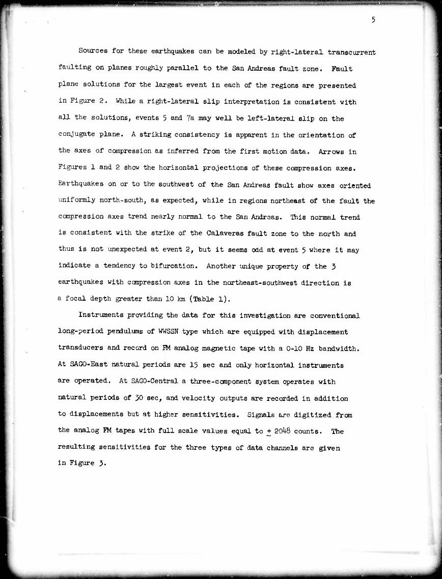
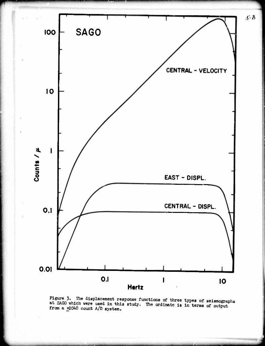
Instruments providing the data for this investigation are conventional

long-period pendulums of WWSSN type which are equipped with displacement

transducers and record on PM analog magnetic tape with a 0-10 Hz bandwidth.

At SAGO-East natural periods are 15 sec and only horizontal instruments

are operated. At SAGO-Central a three-component system operates with

natural periods of 50 sec, and velocity outputs are recorded in addition

to displacements but at higher sensitivities. Signals are digitized from

the analog FM tapes with full scale values equal to + 20^8 counts. The

resulting sensitivities for the three types of data channels are given

in Figure J.

__*^MMa*aB

""■

f-A ^

-p

V

u V bo m

35 i) -p

o ^-

I £ w o ;-

o ;-.

•rH Ü fl

•H u

4) je -p

O r

9 |5a ■p o 0)

• r v f

O

t

3 g o

H

H .Q

ra o oj

I o &l fl -H -P S

g o •H ■P CJ S -i o

u u p< CQ

«

o

w 4)

•a 9

-P

a i 4J fl P >> V

«J

Ö . O 3

■H C

-P

Tl cd

h

Bifl P.P

V aS

3 ai r-i H ft-rl

g o

1-1

-p cd o

•H

s^ V «J

•H CO II

t^S a) a

OJ cd

P */

&:

- ■ ■ ■ — ■ „_

-'"■" ■ I ■

r 100 - SAGO

10

^ ^

o o

0.1 -

0.01

S-h

EAST - DISPL.

CENTRAL - DISPL.

0.1 Hertz

10

?i?S!!Z 3• The di8Placen»ent response functions of three types of seismoKraohs at SAGO which were used in this study. The ordinatc is in ter^s of oS?P

from a jfioW count A/D system. ww*w.

ANALYSIS

Ttie data conBidered in this study are rather unique in that they

axe broadband recordings (bandwidth from .03 to 10 Hz) of ground displacement

n^ar to earthquake sources (epicentral distances from 2 to '40 km). While

there are advantagey to working with data recorded so near the source, there

are also problems not usually encountered in the analysis of far-field

data. Thus is seems appropriate to describe seme general aspects of the

data and the antlyois proceedures which have been applied.

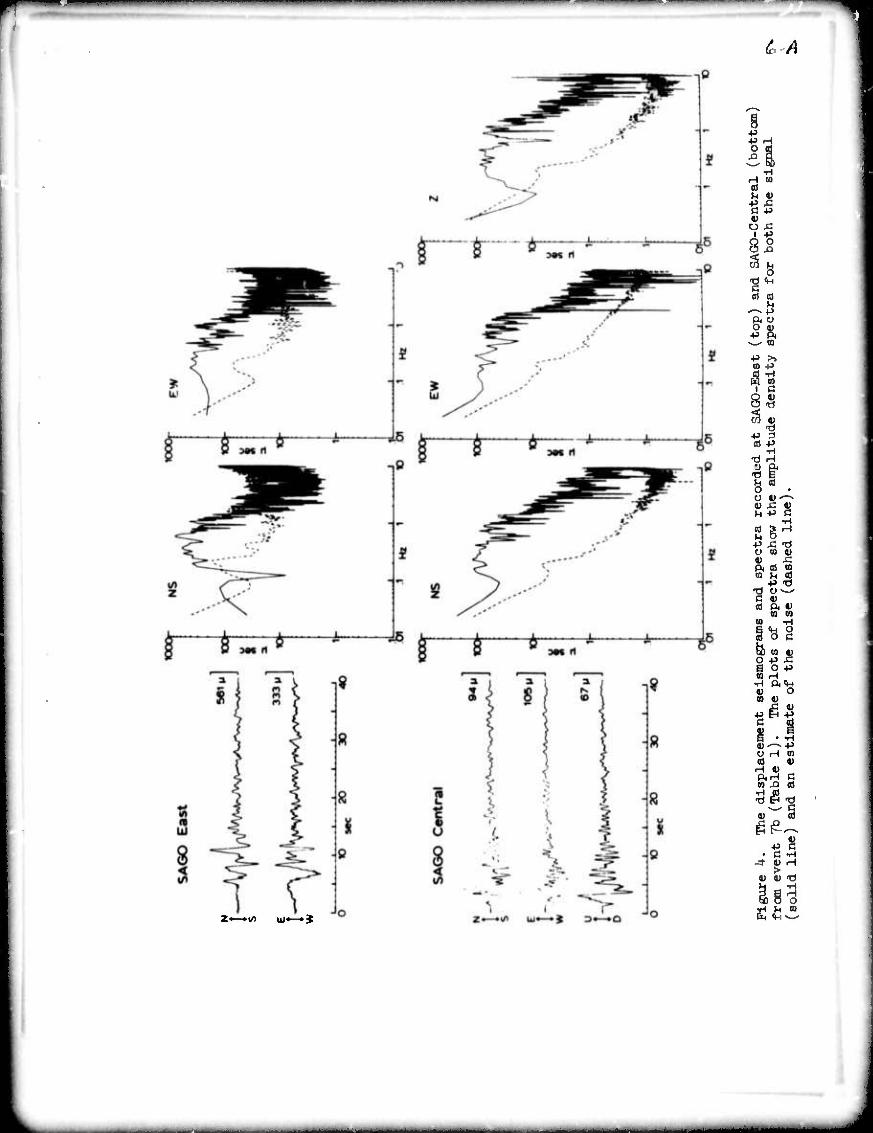
Figure k presents a complete data set for one earthquake. In

the upper part are the time tratSM aril spectra for the

two horizontal components at SAGO-East. The time trp.ces are not corrected

for the instrument response. In view of the broad flat response characteristics

shown in Figure 5 it is clear that these traces closely approximate ground

displacement. Corrections for the seismaneter and all other components in

the data acquisit.on system have been applied to the spectra so they

represent acu.^tl ground displacement. In the lower part of Figure h are

the time traces of displacement and displacement spectra for the three-component

set of instruments at SAGO-Central, As mentioned earlier, the instruments at

SAGO-Central have velocity and displacement transducers at different gains.

During the analysis the velocity output signals are integrated in the

frequency domain with a 40 sec 1 pole high-pass filter simultaneously

applied to eliminate base-line drift. The time tiaces for SAGO-Central

in the figure are such displacement records obtained by integrating th

velocity output signals.

The displacement traces in Figure k illustrate an important characteristic

of near-field seismic data in that the various seismic waves are not isolated

arrivals on the selsmograius. The P wave is typically small but increases

-

-• "■ -' "

&'A

+J ■p —1 Ü 4

rl ■d «i

M a) ■P G n ■P 4) u

3 y o

i ^->y +J A u o | — 1

-p ;-> Ul P

•H

a 6 ^ ^0

^ ■p 3 d

•H Tl rH •) ft

Tl H u CÜ o • Ü 4) -"-> V a 41 U ■p B

2 ^ 3 p d T) C) ■ «1 9) 2 ft 01 CO n u 01

4-> •3 T) t) 1—- G 41 01 P. 41

tn m in •H

tM 0 o a

& ■ 4) 0 +J -C Fi o +J ID H rl P,^ 4) o CD l)

■P i 01

G

8 • 1 i -p r> H en a: 41 H 4> P.H C to XI 03

-d EH Tl

Z«—»CO Ul«—►$

■p 8 • R •H < 41 rH

> ■ 1» Ti

8 i s cu

giH-luaUy until it merges with the much ]uiger S wavt which in turn is

followed by a lengthly and sometimes large coda. Not» that the SAOO-East

station is near a F nodal line so that the P arrival (at about 2 sec in the

figure) is particularly small. It is obvious that it would be difficult to

identify, isolate, and compuce a spectrum for either the P or S wave alone,

and that the truncation effects introduced In such a process could be severe.

For this reason the spectra -«.n this study were all computed from the whole

record with no attempt to isolate individual wave arrivals. The rationale

behind this approach is that all arrivals on the seismoyram, whatever their

mode of propagation, are excited by the same source and thus should carry its

spectral signature. Interference between the various arrivals can be expected

to introduce considerable irregularity into the spectra (usually referred to

as spectral scalloping), but numerical experiments with near-field synthe-cic

seismograms have indicated that the salient features of the source spectrum

are preserved in the whole-record spectra.

All spectra in this study were computed from a hi sec time window which

is the length of the time traces in Figure h. This time window is long enough

to allow the coda to decay to a reasonably small value, ind truncation effects

are further avoided by smoothly tapering the last 2 sec of the time window.

Note that this time window is longer than the significant portions of the impulse

response functions for the 15 and 30 sec pendulums employed in this study. The

spectra are calculated with a discrete form of the Fourier transform defined

in terms of the frequency f in Hz and thus do not involve a normalization

factor of 2 7r (system 1 of Bracewell, 1965, p. 7).

The spectra in Figure k all contain a dashed line which is an estimate

of the nctse present at the time of the earthquake. These estimates were

computed from the time trace during the minute preceding the earthquake.

The analysis procedures for the noise and signal were identical except

that a Henning window was applied to the noise estimate. The solid line

>M mmmtm

-—'■———•'■——

in the plots is an estimate of the amplitude spectral density of the signal

obtained by subtracting the noise estimate frcm the spectrum which was

computed from L^e time trace during the earthquake. The estimate of the

nois« spectrum is helpful in assessing the significance of various features

of the signal spectrum.

The data were sampled at P rate of 50 samples per sec to give a

Nyquist frequency of 25 Hz. The analog signal was strongly filtered

beyond 10 Hz to avoid aliasing and noise problems (see Figure 3). Spectral

estimates at frequencies above 10 Hz consist of a small signal strength

magnified by a large instrument correction factor (particularly in the case

of the displacement channels) and are considered less reliable than those

at lower frenuencies. For this reason frequencies above 10 Hz are not

considered in this study. At low frequencies tie affect of the instrument

correction is not so pronounced and all spectral estimates falling above

the noise level are considered to be reliable. However, as will be

discussed later, the conventional long-period instruments employed in

this study are susceptible to tilts and spurious transients which affect

the low frequencies, so considerable care must be taken in interpreting

this part of tbi spectrum. Tht type of vertical seismometer at SAGO-Central is

known to be susceptible to nonlinear parasitic vibrations during strong

shaking, and thus data from this instrument have received much less

emphasis than those of the horizontal cooiponents.

The spectra obtained in this study are amenable to the usual int rpretation

in terms of low-frequency level, corner frequency, and hi^i-frequency slope.

The spectra are typically feirly flat in the frequency range 0.1 to 1 Hz

and the low-frequency level, r^, was estimated frcm this portion of the

spectrum. At frequencies less than 0.1 Hz the spectra are much more

variable (see, for example. Figure k). Beyond about 2 Hz all of the spectra

■1

show a pronounced decrease with increasing frequency which is fairly linear

on a log-log plot and typically has a slope of about -2 to -3. In Figure k

the spectra from the displacement transducers reverse their slope and begin

to increase beyond about 5 Hz, but this is clearly due to the presence cf

noise,

Several different approaches to the problem of esoimating the spectral

characteristics of low-frequency level, corner frequency, and high-frequency

slope were investigated, and the one finally used and described here seemed

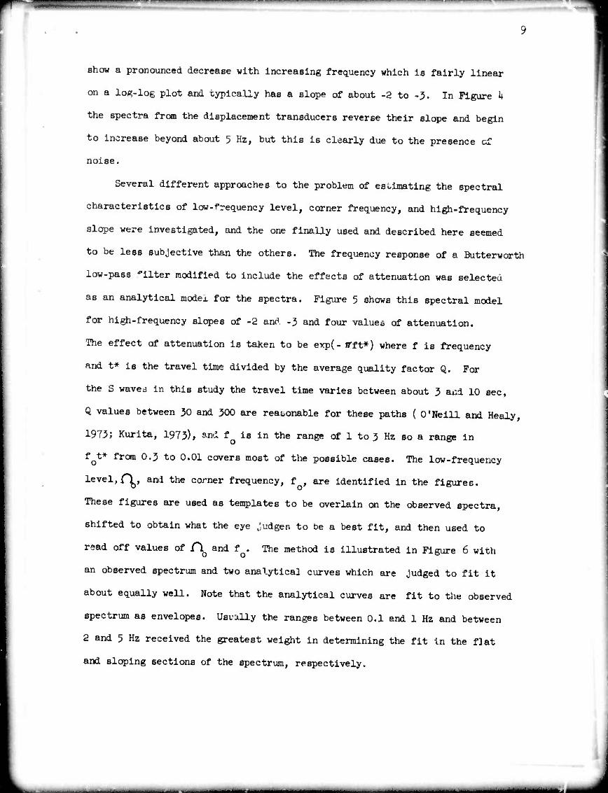
to be less subjective than the others. The frequency response of a Butterworth

low-pass -"ilter modified to include the effects of attenuation was selected

as an analytical modex for the spectra. Figure 5 shows this spectral model

for high-frequency slopes of -2 and -3 and four values of attenuation.

The effect of attenuation is taken to be exp( - nrft*) where f is frequency

and t* is the travel time divided by the average quality factor Q. For

the S waved in this study the travel time varies between about 3 aud 10 sec,

Q values between 30 and 300 are reasonable for these paths ( O'Neill and Healy

1973; Kurita, 1973), »»i f is in the range of 1 to 3 Hz so a range in

fot* from 0.3 to 0.01 covers most of the possible cases. The low-frequency

level,r^, and the corner frequency, f , are identified in the figures.

These figures are used as templates to be overlain on the observed spectra,

shifted to obtain what the eye Judges to be a best fit, and then used to

rsad off values of Ao and f . The method is illustrated in Figure 6 with

an observed spectrum and two analytical curves which are Judged to fit it

about equally well. Note that the analytical curves are fit to the observed

spectrum as envelopes. Usv-Oly the ranges between 0.1 and 1 Hz and between

2 and 5 Hz received the greatest weight in determining the fit in the f]at

and sloping sections of the spectrum, respectively.

'■'■«■■ '

. . 9-A

1 — * —• 1 ' *•''•■• i i

1 —• 1 I

>l r C 4J : cr a) H fj

h^ S <^ | O

n LI 41

4' 3 £_ rH

+J 01 >

01 ^ 0 i..

c: b o H Cn 4) > T)

^ C^

> ^^ C) +J

4) a 3 vH n« M 4J G

4H ">

B --i . H d

01 a) a '—^ H •p

C. <VH 4' 0 rH ^-^ ■ o 0,l p 1

i ■ •iH •H ■P W 4J 1) 5)

o H H 01 U3 E «J ^> C) ') 4J C ^ 41 m n

n< v: 4)

•H h (rt Vi

■P i ^J B a Eb

•H o jd M ■ Tl J2 ID JJ UJ 3 4)

>H w 4) a) v: M ;» 3 ■ i a; 01 l-i u

4) • C iri+J

4' 1 I o

■ MVOi ^"'

10000 high frequency slope

-2

1000

u CD

100

fot .3 .1

M

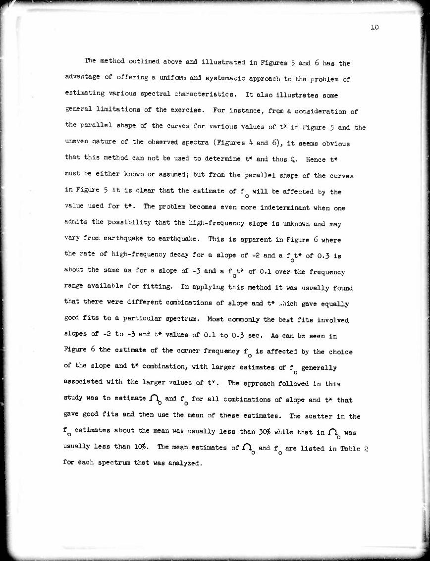
Figure 6. Example illustrating two different estinntes of the low-frequency levelO and the corner frequency f of the spectrum from the NS conrrcnent at SAGO-East from event 6 (Table l):

10

The method outlined above and illustrated in Figures 5 and 6 has the

advantage of offering a uniform and systemacic approach to the problem of

estimating various spectral characteristics. It also illustrates some

general limitations of the exercise. For instance, from a consideration of

the parallel shape of the curves for various values of t* in Figure 5 and the

uneven nature of the observed spectra (Figures 4 and 6), it seems obvious

that this method can not be used to determine t* and thus Q. Hence t*

must be either known or assumed; but from the parallel shape of the curves

in Figure 5 it is clear that the estimate of f will be affected by the

value used for t*. The problem becomes even more indeterminant when one

adxuits the possibility that the high-frequency slope is unknown and may

vary from earthquake to earthquake. This is apparent in Figure 6 where

the rate of high-frequency decay for a slope of -2 and a f t* of 0.5 is o

about the same as for a slope of -5 and a f t* of 0.1 over the frequency

range available for fitting. In applying this method it was usually found

that there were different combinations of slope and t* -hicn gave equally

good fits to a par.icular spectrum. Most commonly the best fits involved

slopes of -2 to -3 •nd c* values of 0.1 to O.J sec. As can be seen in

Figure 6 the estimate of the corner frequency f is affected by the choice

of the slope and t* combination, with larger estimates of f generally

associated with the larger values of t*. The approach followed in this

study was to estimate f\ and f for all combinations of slope and t* that

gave good fits and then use the mean af these estimates. The scatter in the

fo estimates about the mean was usually less than 30^ while that in Cl was

usually less than 10^. The mean estimates of A and f are listed in Table 2 o o

for each spectrum that was analyzed.

11

In aad'tion to the conventional spectral Btudles described in the

foregoing paragraphs, the data of this study afford the opportunity of

studying the earthquake source In the time domain. Using the location

and fault plane data in Table 1 and assuming a point dislocation imbedded

in a halfspace as an earthquake model, it is possible to calculate synthetic

seismc-rams (Johnson, 197^) which can be compared with the observed seiamograms.

While this model c.f tlM earthquake source is undoubtedly oversimplified, it

does have the advantages of allowing an exact analytical calculation which

includes both near-fiela and far-field terms and containing only two free

parameters, tue monent and rise time of the dislocation. These two parameters

enter into the problem more or less independently, as the rise tlM is related

to the width of the seismic pulse (and the corner frequency in the spectral

domain) while the moment is related to the amplitude of the seismic pulse

(and the low-frequency level in the spectral domain). Thus the synthetic

seismogroms provide an independent means of estimating some of the earthquake

source parameters.

The velocity difference across the San Andreas fault zone (discussed

earlier) was incorporated into the calculation of synthetic seismograms

in an approxiinate manner by assuming the average P velocity of the halfspace

to be 5.5 and 5A km/sec for paths to SAGO-Central and SAQO-East, respectively.

The S velocity was inferred from the P velocity by assuming a value of 0.25

for Poisaon's ratio, and the density was taken to be 2.67 gm/cm3. The time

history of the dislocation was taken to be a step function with a finite

rise time (time to reach the final dislocation value) such that the function

and its first derivative are continuous everywhere (Litehiser, 1974). This

means that the spectrum of the body waves radiated fron this source wlU have

a high-frequency slope of -2 in the far field.

ttmmm

.TU

The synthetic seiamograms also provide a simple method of attacking

a troublesome problem of near-field studies, the effect of tilts and

spurious transients. All horizontal seismoneters respond to tilts and

at low frequencies the output of near-field seismüoieters resulting from j

ground tilt can be comparable to that resulting from ground displacement.

There is no simple way of separating the two effects since horizontal

acceleration due to tilt is indistinguishable from that due to horizontal

displacement. However, synthetic seismograms due to ground tilt can be

calculated in the same way as synthetic seismograms due to ground displacement

and a comparison of the two gives a measure of the tilt effect for the source

model used. The inference is then made that a similar effect may be present

in the observed seismogram. This approach is rather qualitative but it

has proved to be useful in analyzing the low frequencies in the observed

spectra.

- -

— »"■"••Ill

13

DISCUSSION

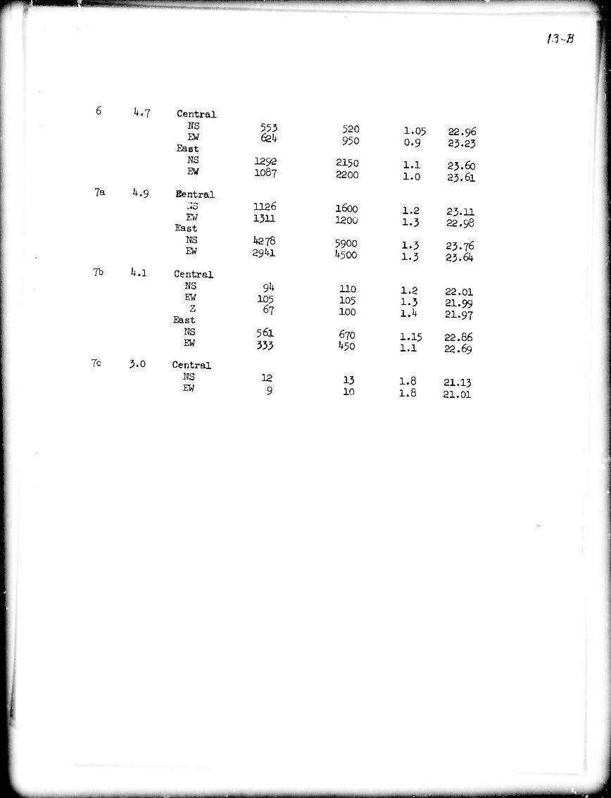
Table 2 Is a sunnnary of measurementB obtalnec for the earthquakes listed

In Table 1. Results are given for all components which recorded useable data

from each earthquake. The maximum ground displacements are measures of maximum

amplitude on displacement seismograms. Prior to this measurement the signals

were filtered (2 Hz 1 pole low-pass) to remove high-frequency noise la the

case of displacement transducers, and the signals were integrated in the case

of velocity transducers. The spectral estimates of H and f were obtained o o

with the method outlined in the previous section.

The low-frequency level ("^ was converted to an estimate of the seismic

moment M using the formula o

MO = kirpßhc\ (1)

where fi is the density, ß is the S velocity of the medium, and R is the

hypocentral distance. This formula assumes that A is calculated from a

far-field S wave, that the free surface effect can be ignored, and that the

radiation pattern has no effect. Although none of these assumptions is

strictly valid as used her?, numerical experiments with whole-record spectra

of synthetic seismograms fron sources with known M have indicated that this

formula is reasonable for estimating the seismic moment with near-field data.

Consideration of the seismic manents listed in Table 2 shows that the

values estimated at the SAGO-East site (located on Pliocene sediments) are

always greater than those estimated at the SAGO-Central site (located on granite)

for the same earthquake. On the average they differ by a factor of about 5.

This difference is most likely due to the effect of geology at the recording

site as it is seen for events in all source regions and appears to be Independent

of azimuth and distar-e to the earthquake. This observation of larger amplitudes

on sediments than on basement rocks is fairly cc^ion in seismology (Gutenberg,

•— m~ ■■ ■■ ma —

Able 2. Summary of measurements obtained fr

and displacement spectra

am displacement seismograms

/3~A

Event \ Component Maximum ground

displacement M

no fo lo^V M-sec Hz dyne-cm

^.6

3b

3c

3d

^a

hb

h.l

k.O

2.6

3-7

2.4

5.1

3.6

4.7

Central N3 EW

East NS EW

Central NS EW

East EW

Central NS EW

East NS EW

Central NS EW Z

Central NS EW Z

Central NS EW

Central NS EW

East NS EW

Central NS EW

Central NS EW I

2847 2918

3117 3690

329 751

27^6

144 116

674 456

4 6 h

90 90

59

5 5

1225 1241;

2657 3208

21 20

108 158 134

1500 930

2600 4ooo

337 430

1500

1-3 1.4

1.4 1.2

1.7 1.7

2.1

23.22 23.01

23.43 23.61

22.60

22.71

23.15

210 190

1.3 1.4

22.37 22.32

1500 690

1.6 1.6

23.27 22.93

3 4 2

1.9 1.9 2.0

20.51 20.64 20.43

150 x30

75

1.1 1.1 1.2

22.19 22.13 21.89

2 2

1.9 1.8

20.33 20.33

3000 2700

1.0 1.0

23.87 23.82

5500 8000

1.4 1.2

24.14 24.31

22 26

2.6 2.2

21.68 21.75

200 320 210

1.4 1.2 1.4

22.82 23.02 22.84

■■ '"

n-n

h.l

7a ^.9

To ^.1

Tc 3.0

Central NS EW

East

553 621+

Ni3 EW

1292 1087

Bentral 3B n?6 EW

East 1311

NS EW

1*278 29^1

Central NS EW

Z East

9h 105

67

NS EW

561 333

Central NS EW

12 9

520 950

1.05 0.9

22.96 23.23

2150 2200

1.1 1.0

23.60 23.61

1600 1200

1.2 1.3

23.11 22.98

5900 4500

1.3 1.3

23.76 23.61+

no 105 100

1.2 1.3

22.01 21.99 21.97

670 U50

1.15 1.1

22.86 22.69

13 10

1.8 1.8

21.13 21.01

~M^m^m*

■' ■ ■ ■ 1 II ■ ■ I '^mmrmH

Ik

1956a, 1956b, 1557), although one might expect the differer.ee to vanish toward

Zero frequency. An alternative explanation is that the strong lateral contrast

in crustal properties across the fault zone causes an asymmetric distribution

in both stored and radiated elastic energy. This latter explanation would

ünply that studies of this type are capable of defining the absolute slip

on each side of the fault.

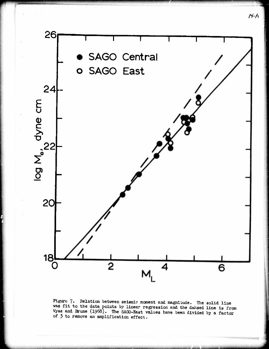
Figure 7 shows log(Mo) from Table 2 plotted as a function of Wood-

Anderson magnitude M^ Each point represents the average log(Mo) obtained

from the horizontal instruments at a given site. In constructing the plot

the moments at SAGO-East we.e all divided by a factor of 3, so the plot can

be considered appropriate for bedrock southwest of the San Andreas fault. The

solid line was fit to the data points by linear .egression analysis and has

the equation

log(Mo) = (17.60 ♦ .28) ♦ (1.16 + .06) * (2)

The dashed line is the relation derived by Wyss and Brune (1968) for San

Andreas earthquakes with magnitudes less than 6 and has the equation

log(Mo) - 17.0 + 1.4 |L /-j

The main features of Figure 7 are the very linear log moment-m^tude relation

and the good agreement between the data of this study and the results of

Wyss and Brune (1968) in which the moments were estimated on the basis of

surface wave amplitudes and field evidence. Both of these features support

the contention of this paper that whole-record spectra of near-field

seismograms yield reliable estimates of the seismic moment.

In the case of the corner ^equencies fo listed in Table 2 there does

not appear to be a systematic difference between the values estimated at

SAGO-Ontral and SAQO-^st for the same earthquake. Ofcus all estimates

of fo for a given earthquake have been averaged in order to obtain the

Plots of log(fo) versus both ^ and log(Mo) shown in Figure 8. Linear

I 1 ' ' -'■" ■' -

/V-/i

26

24 E u

c

,22

o

20

18 0

T 1 1

• SAGO Central o SAGO East

Figure ". Relation between seismic moment and magnitude. The solid line was fit to the data points by linear regression and the dahsed line is from Wyss and ßrune (1968). The SAGO-East values have been divided by a factor of 3 to remove an amplification effec\.

-^.^.

■i^"^""1111 "" '• ••••mi i.nii.ii mmmmmm^mm • nil iiniiiii» i i i 11

15

regression analysis of the data points in these plots yields the equations

log(fo) = {OM + .12) - (0.079 + .030) IL (4)

and

log(fo) = (1.80 + .52) - (0.073 + .023) :-Og(Mo) (?)

Thr considerable scatter in the data points of Figure 8 is reflected in

the rather large uncertainties associated with the slopes and intercepts

of these least-squares lines. The present data do not allow any strong

conclusions to be drawn concerning the existence of a systematic relation

between fo and either ^ or Mo. However, the general trend of the data

points and the slopes of the regression lines in Figure 8 suggest that

fo is only weakly dependent upon either M^ or M for these central

California earthquakes of small to moderate magnitude.

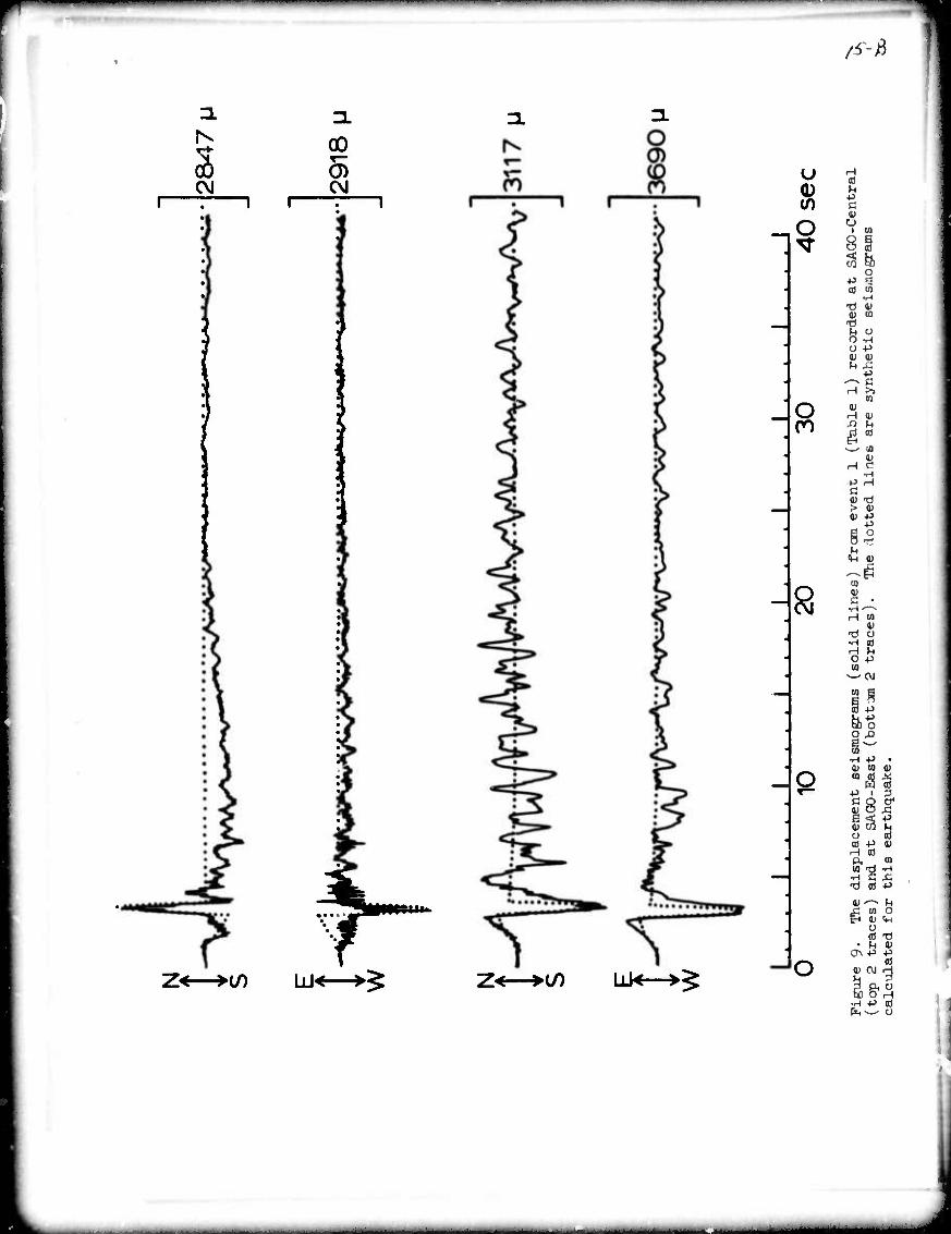
Considering now the individual earthquakes, it is convenient to begin

with event number 1 which is the earthquake nearest to SAGO.

The epicenter is east of the main trace of the San Andreas fault. On

the basis of the compression axis indicated by the fault plane solution

it appears to be associated with the Calaveras fault (Figure l). Seismograms

recorded from this earthquake (Figure 9) are fairly simple records, beginning

with an emergent P wave and a gradually increasing disturbance

interupted by a large unipolar S pulse followed by a relatively small

amplitude slowly decaying coda.

The dotted lines in Figure $ are synthetic seismograms calculated

for this earthquake according to the method outlined in the previous section.

For the purposes of the calculation the fault plane solution given in Figure 2

and Table 1 was used but the epicenter was moved 1 km south from the location

given in Table 1 in order to achieve agreement between the observed and

calcula'-ed first motions of the P waves. This adjustment of 1 km is within

—^—.^

——————————————— —

/5v}

22 lo9 MOJ dyne cm

24

Figure 8. Relation between corner frequency and magnitude (top) and between corner frequency and log moment (bottom). In both graphs the line was fit to the data points by linear regression.

—

/^

5 CVJ

Z<—>V) u< >^ Z<—>(/) UK—►$

Si o

O

8

i

8 8s a

o ■p I to ra

f-i

0) (0

o o +> D V M £

H >> CO

u

.rj II

id n

a > a> 0) -P

p

h

m V ß •

•rH ^~» H M

V T) Ü

d H o +> CO

§s CO P

o a CO

to TJ •H ß

2 M H D o

(0 • u a\ p

4) OJ

E& •H P

II .X cd

& .c p

6 a

•H G P b o

ID ■P

3 u d ü

•MMMriMMMMMMfe^^M

«■■■"■ —'—'-

16

the uncertainty of the epicenter location. A rise tüne of O.67 sec was

used for the source function.

In their general features, the observed anc synthetic

seismograms in Figure 9 are fairly süniiar. First motions of the

P waves are all in agreement, although it is difficult to see in the

figure that the first motion on the EW synthetic seismogram at SA30-Central

is actually in the W direction. The S - P intervals are in agreement and

the directions und shapes of the S pulses are quite similar. The portions

of the seismograms between the beginnings of the P and S waves, which are

mainly the contribution of the near-field parts of the solution, are in

reasonable agreement at SAGO-East but at SAGO-Central there is an obvious

discrepancy which has not yet been explained. Because the synthetic

seismograms were calculated for a homogeneous halfspace, they are incapable

of matching the coda that follows the S pulse on the observed seismograms.

The major features on both the observed and synthetic seismograms are

the S pulses. Note that, just as in far-field calculations, the shape of

the S pulse on the synthetic seismograms is essentially the derivative of

the source time function. The duration of the S pulse can thus be interpreted

as an estimate of the rise time of the source function. At SAGO-Central the

duration of the observed and synthetic S pulses are in good agreement. At

SAGO-East it appears that the agreement could be considerably improved if

the rise time were increased from O.67 sec to about 1.0 sec, but such a

change would destroy the agreement at SAGO-Central and it would also degrade

tim fit between the observed and synthetic spectra (Figre 10). An hypothesis

cnat attributes the increased duration of the S pulse at SAGO-East to the

superposition of two or more S pulses seems to be the most reasonable

explanation at the present time. A major discontinuity, the San Andreas

. . _.

mm —'

lOOOOr-

1000-

s -1

100-

10-

01

10000-

1000-

i in

100-

10-

01

^J_ HZ

' ' ' l\ ' W , ' '1. » , •?.«

.-^_

IOOOOI-

1000-

u x

100-

10-

J 10 "01

10000-

1000-

%

10CH-

io-

HZ 10 01

EW

_— I

EW

_J.

HZ

I

10

Hz io

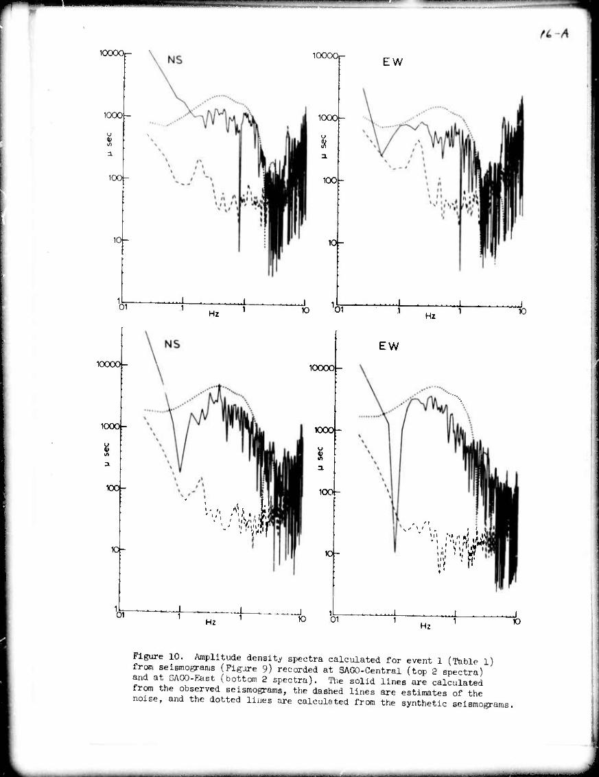
Figure 10. Amplitude density spectra calculated for event 1 (Table 1) from seiEmogranis (Fig-ore 9) recorded at SAGO-Central (top 2 spectra) and at SAGO-East (bottom 2 spectra). The solid lines are calculated from the observed seismograms, the dashed lines are estimates of the noise, and the dotted lines are calculated from the synthetic seismograms,

r-w«

17

fult, lies U:t.„n the tyo 8taUon8 and ^ ^ ^^^^^ ^ ^ ^

effect

^ . =on8M„aUo„ or the UM dcrain alone. ^ „^^ ^ ^^ ^

a^Un« th. eou.o. n<)nent of the .^.^ ^^^ ^ ^ ^^

°f the S pul8e on th. s.nth.Uc Mfogr« «toh.. that on th. observed

-i^a.. s„=h t^e-^in ..t^f. or th. ^ent „ere „btalned for each

exponent of r.^a ^ „otlon ana th. .eauita ara Hated !_ T.ble j

^e spectra canted fro. the seU^a.a of Figure 9 are shown In

n^ io. ^ lnu8trate 6n()ther „^ of estimtin6 ^ ^^^^ ^^^

-ent. !„ m. ease the „cent of the esthetic earthy fa adjusted

-tU the synthauo speotr,. u a reaso.hae m to the ohserved speotru..

Such fre^.do.adn eatlmtea of the Ment .ere ohtained for each c„pone„t

of recorded «round „otlon and the result, are listed In T^ie J

-Of that the effects of radiation pattern, free s„f.ce, and propa.tlon

are all Incorporated vhen the synthetic calculations are uaed to estate

the selaMc .»ent In either the tl- do^ln or frequency dc^ln. The

-dlat.on pattern Is particularly Important for event 1 hecause It la a

str^-sllp earth^e located al„oat directly helou the recording stations,

- thus It is not aupnalng that the Ment estl^tea In ^u 3 are heater

the radiation pattern, „so note that the effect of attenuation has not

haen Included In the synthetic calculations, althou^ It could he done

given an appropriate value of Q.

An interesting feature of the spectra m n^e 10 deserving father

attention 1, the rise In the ohserved spectra .ovard th. lo. freund,.

The synthetic spectra do not aho« thla feature. A posslhle option

■

■ ■M II ■■ ■-«-■

Table 3. Seismic moments determined with the aid of synthetic seismograras

Event ■\

Rise Time Component Time Donain log(M )

Frequency Dnmnin log(Mo)

k.6

sec dyne-cm dyne-cm

1 O.67 Central NS EW

East

23.51 23.47

23.67 23.65

NS EW

23.83 23.76

24.30 24.19

2 4.7 0.50 Central NS EW

East

22.83 22.54

23.05 22.77

EW 23.18 23.48

4a 5-1 1.00 Central NS EW

East

23.19 23.25

23.67 23.81

NS EH

23.66 23.62

24.16 24.17

7a 4.9 O.67 Central NS EW

East

22.65 22.95

23.06 23.03

NS EH

22.69 23.25

23.53 23.82

n-A

■ ■

of this difference involves the tilts associated with the seismic waves

which appear as apparent accelerations to the horizontal seismometers.

Ac a check on this possibility the synthetic seismograms resulting from

elastic tilts were calculated and are shown in Figure 11. The total

synthetic seismogram can thus be obtained by adding these tilt-induced

records to the synthetic records resulting from displacements (dotted

lines in Figure 9). The primary effect of the tilts, which retain static

values after passage of the waves, is permanent offsets on the seismograms.

In this particular case, however, the offsets are small compared to the

maximum displacements and have a very small effect upon the synthetic

spec era. While synthetic tilts calculated for an elastic halfspace model

are too small to explain the discrepancy between the observed and synthetic

spectra, it is possible tht.t the use of a more realistic model with vertical

inhomogeneities could lead to an amplification of the synthetic tilts.

However, regardless of the model employed, the primary effect of the elastic

tilts will undoubtedly be permanent offsets on the seismograms, and an

inspection of the observed seismograms in Figure 9 indicates that this is

not likely to be the required solution.

The primary discrepancy between the observed and synthecic seismograms

in Figure 9 is a long-period transient feature in the observed seisuograms

that reaches a maximum some 5 to 10 sec after the S wave. The shape of

this feature, which is best displayed on the NS component at SAGO-Central,

suggests that it could be explained as the instrumental response to an

impulse in tilt. This is confirmed in Figure 12 which is identical to

Figure 9 except that the response due to an impulse in tilt has been

added to the synthetic seismograms. The impulse in tilt was assumed to

occur at the arrival time of the S wave, had a duration of O.67 sec,

18

r1"1'! "

■"—■■■ " -1 " ■ -— "

f8 A

0) T i 1

if) (0 i 1 i 2K' CO

O

o

a

UM—♦$

-O

1 0) H U

ß o

•H

71 o

(0 4J CJ

to E -»>

8<H

to R -p

R 0)

I

cd

■ PH-P

5 o

u

tä e u CD H

q •H

a; ■

ij %o a H

p

m

i •H

ft Of i

u ja ■p

o ■ -p ;3 o, p

o

5^

P i co i) u

O -H P ri

p< to p

V p o CVJ •H

0) Ö M p P.P

o

I) ,r:

I 3 to o

u

1) to

p

P p o

0) O 0) -H ' < J3 P

W P Ö 0)

fe aJ O -H

a

M^UMMMHHMi^flMI

/M

S 00

CsJ

•CO UJ^

u 0) iT)

CO

"

C\i

_o

^ c oo cd II (d -p

OJ ON

o< 1) 4-> 3

c

8 1 ■P -H a) a> ■

•P 4) 0) >

y x; cd (U p > h c

>> to ^> to H 1)

a; x: U -C P H P

o

£a

s 0)

r-l W -r-i 01 P

P 9 a> H td > 0) -0 i E P O P M o

§^P ft ro

0 • p S^H 0) 10 -rl •H 0) P V U M a) c

^ -H P P C V 01 OJ OT B H 4) g P o a a, cd p s H P -3 P. o to X) oi

■y -H p p

1' CO ü] tP to ED

• ^

o

p b cd

fc cd (S

IOOOOI-

1000

Si

100

10-

01

10000-

DOO-

10O-

K)-

01

— J. Hz

Hz

lOOOOr

1000

3!

100

10

10 .01

10000

1000

3.

100

10

10 .01

EW

EW

I

I HZ

ITT

HZ

S^üi«* ^P11*^6 density spectra calculated for event 1 ^Table l) The solid and dashed lines are identical to those of Figure 1C but t^e' *? tV1?*8 are calculated fom the synthetic seismogr^ of Fi^re L

which include the effects of an impulse in tilt

/?-c

I 10

10

-

1^

a.id had amplitudes of -87, -20, -lOk, and -29 mlcro-radiariB on the components

SAGO-Central NS, EW, SAGO-East NS, and EW, respectively. The spectra are

given in Figore 13. Ccmparing Figures 12 and 13 with 9 and 10 shows that

an impulse In tilt is capable of explaining the discrepancy between the

observed and Lynthetic seismograms. But the cause of such an impulse is

not explained by this exercise and a number of possibilities exist. The

possibility that it is a direct effect of the earthquake source which

was not included in our simple synthetic model seems unlikely, but it

can not be completely ruled out. The possibility of a nonlinear instrumental

effect such as a rocking, sliding, or flexing of the instruments during the strong

ground motion of the earthquake seems more likely. In any case, it is clear

that considerable care must be taken with the interpretation of near-field

spectra at low frequencies.

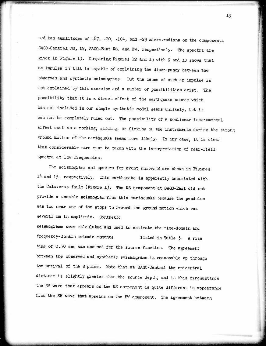
The seismograms and spectra for evr.nt number 2 are shown in Figures

Ik and 15, respectively. This earthquake is apparently associated with

the Calaveras fault (Figure 1). The NS component at SAGO-East did not

provide a useable seismogram from this earthquake because the pendulum

was too near one of the stops to record the ground motion which was

several mm in amplitude. Synthetic

seismograms were calculated and used to estimate the time-donain and

frequency-domain seismic moments listed in Table 3. A rise

time of 0.50 sec was assumed for the source function. The agreement

between the observed and synthetic seismograms is reasonable up through

the arrival of the S pulse. Note that at SAGO-Central the epicentral

distance is slightly greater than the source depth, and in this circumstance

the SV wave that appears on the NS component is quite different in appearance

from the SH wave that appears on the EW component. The agreement between

^__11—_^_. ■HiiaHHHMMMMHi

/?-/?

o CVJ

-P

-•o

H -ö cd 0)

-P (0 a; 3 o ■ o

d o

ca G td

q

U3

8 <

01

OJ

o u II

CJ

P G h co

-O

4) E OJ CO

P G

N O 0) ^1 p

<^l p o

■

3fl

o o CO CD

^— U ■P ■

2 0

+» to

A i

8 8S

V}

p c OJ E o u a) H P A cd n

•H tj T) G

cd t

-4 rH

U OJ

I)

S o' p h IB

fl

rC P o

--■ . -

rt^W

1000 1000(-

Figure 15. Amplitude density spectra calculated for event 2 (Table l) from seismograms (Figure lU) recorded at SAGO-Central (top 2 spectra) and at SAGO-East (bottom spectrum). The solid lines are calculated from the observed seismograms, the dashed lines are estimates of the noise, and the dotted lines are calculated from the synthetic seismograms.

20

the observed and synthetic spectra is also reasonable, although the noise

level at SAQO-Central is large enough to obscure much of the hi^i-frequency

behavior.

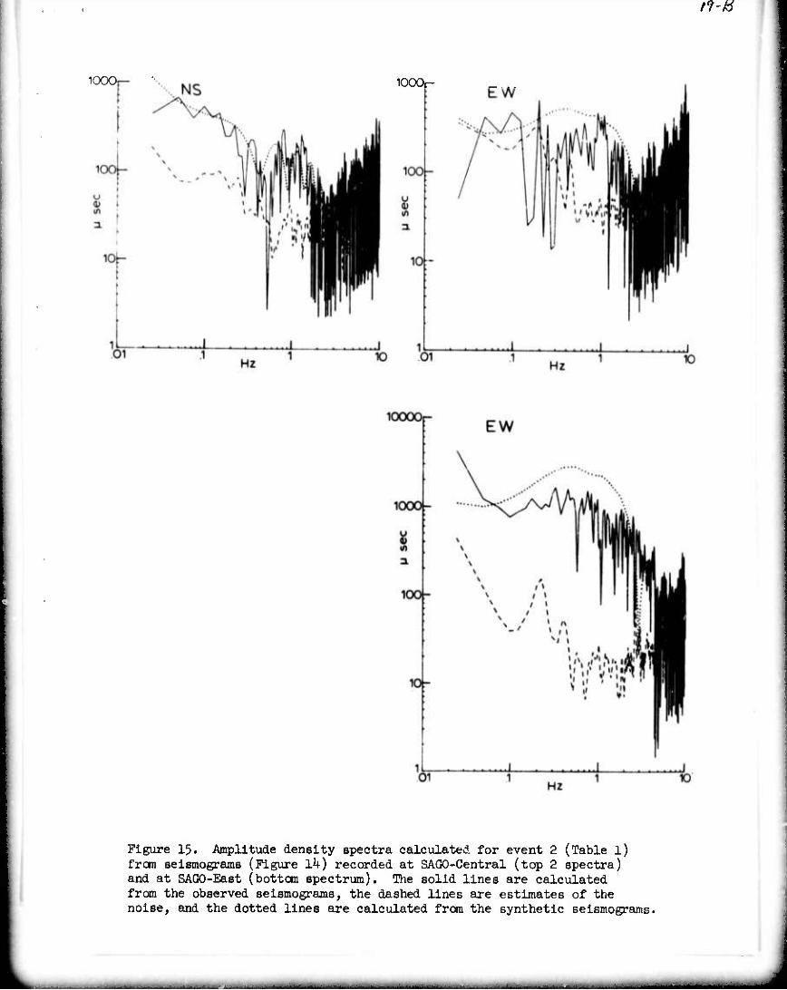
The seismograms and spectra for event number 7a are shown in Figures

16 and 17, respectively. In terras of both location (Figure l) and fault plane

solution (Figure 2) this earthquake appears to be associated with the

Pinecate-Vergeles fault complex io the west of the main trace of the

San Andreas fault. Synthetic seismograms and spectra calculated on the

basis of this location and fault plane solution ana a rise time of O.67 sec

are also showi. in the figures and were used to calculate the tlme-dcenaln

and frequency-domain seismic moments listed in Table 3. In terms of general

features the observed and synthetic results are in fair agreement. The

comparison between observed and synthetic seismograms at SAGO-Central

indicates that the waves have approeched the station from a more northerly

direction than implied by the synthetic calculations, and this could arise

from either a small Inaccuracy in the epicenter location or curvature in

the wave paths due to velocity inhomogenelty. At SAGO-East the largest

amplitudes on the seismograms occur several seconds after the arrival of

the S waves. This unusually large coda may be associated with the fact

that in travelling to SAGO-East the waves have passed fron material with

higher velocity and lower vertical velocity gradient west of the San Andreas

fault into material with lower velocity and higher vertical velocity gradient

east of the fault. Note however, that this phenomenon does not appear when

the waves cross the fault in the other direction a! in the case of the

seismograms recorded at SAGO-Centnl from events 1 and 2 (Figures 9 and Ik).

Another interesting aspect ox this earthquake is the fact that the

rise time of O.67 sec which gives a reasonable fit between the observed

and synthetic spectra (Figure 17) is too short to explain the duration

.MMM

JLV ^n

(0 CvJ

00

'.'A.

I/) UJ^—►$

5! 1^

o 00

8

•n

a) co | I a y 0 H O (0

1 o

8 ui

a o _ E -ö W

•n a» o o o

H H5 a-

ß

c ■ a- a

u :• li ■I1 i

I

m <H ü H (0 O JH (0 -p

fi o o B XI «^—- a -p CO to

8 -p c L- OJ o a) H -P A CO •

d "a 5 T) C a)

td 2 0) O*

tn to -p 0) U Ü

P Vi'

a'

D aj

I m

•H

P

?o #

10000p

1000

u <x> U1

lOOH

10-

lOOOOr-

1000-

0) in

100-

10-

1cii—-

NS

/1

i.-' , ■ i

■• < i

1 Hz

lOOOOr

1000

in

100-

10-

fe v

10000,

1000-

EW

K)

HZ

....I 1 10

21

of the large S pulse. This is best observed on the SAGO-Central recordings

in Figure l6, and a similar situation exists on the SAGO-East seismograms

from events 1 (Figure 9) and 2 (Figure Ik). As mentioned earlier, it

appears as if the S pulse actually consists of the superposition of two

or more pulses. Calling upon seme source-related phenomenon such as

finite source size to explain these features seems reasonable, but such

a hypothesis is challenged by the results shown in Figure 18. This figure

compares the seismograms recorded at SAGO-Central from event 7a with those

recorded from two other earthquakes in the same source region, events 7b

and 7c. The important point is that, even though these 3 earthquakes cover

a magnitude range of almost 2, the seismograms have a very similar appearance

The length of the S pulse does not show an obvious dependence upon the

magnitude of the earthquake, which argues against it being caused by the

source itself. An alternate explanation which seems more acceptable at

the present time would attribute the multiple nature of the S pulse to

wave propagation effects due to inhomogeneities along the path between the

earthquake and seismometer.

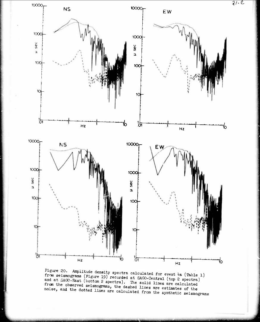
Next consider event number ha for which the seismograms and spectra

are shown in Figures 19 and 20, respectively. The synthetic results in

these figures were calculated assuming a rise time of 1.0 sec for the source

function. The fault plane solution for this earthquake gave a strike of

N55W for the fault plane (Table 1). However, in order to explain the first

motions of the P waves a strike of NU5W, which coincides with the strike of

the San Andreas fault in this region, was used in the synthetic calculations.

Comparison of the observed and synthetic seismograms in Figure 19 shows

considerable contrast between SAGO-Central and SAGO-East in spite of the

fact that both stations are at approximately the same distance and azimuth

-

N

JCUV

w

1126 M

94 M

12 M

-1 ' ' ' ' ' ' ■ ' 'J ■ ■ ■ ■ ' ' ' I . . ■ I ■ ■ ■ . I ■ ■ ■ I , , , | O 10 20 30 40 sec

^LY,/^V>ä^^^ 1311 M

105 M

0 10 ■*, ^ ' ■ ■ ' ' ■ ■ ■ ■ I ■ ■ ■ ■ I • - I 20 30 40 sec

üf^vo8'^6 ^^f"111611* sei8m^Äram8 recorded at SAGO-Central fron event 7a, 7b, and 7c (Tfeble l) with magnitudes 4.9, 4.1, and 3-0, respectively.

irr

C\J

CsJ

Z<—>C0 lü<—>$

-■ i H +i

u cd er P (D U) o o)

O 1 o

O CD ^r ^ 4J Ö) (0 o 1 -d u JJ -H T) (U h M O O CJ OJ -H U -P

u — x: H -P

ß 4) >.

o X)

00 £S i; c -P -H c ^< II > T) U u

P e p o o ^ -d

'+H V

in e<

o § C\J H^

(0 ■Ö 0) •H CJ H cfl o u tn p

(M (0

§ § || o o S -a m^ •rl (U 4J cn oi o C i

%8 i r-t P P. cö • (0 v •^ -O -*

^g? tt» o1

p'w P V u o cd

• a a» ON k. H P M

r^\ •H <J 9' j w:

•H P O

lOOOOr

1000-

V in

100-

10-

01

NS

■ . , I

KDOOOr-

Hz -^- * ■ ■ !_

1000-

i

lOOi-

10-

io 'oi

EW

i—i - ■ 11ni

1 HZ 1

l/~t

lOOOOt-

1000»-

10000

1000-

Ü

100-

10-

01

EW

Hz

fiSTL?0" Anipii!iude denaity spectra calculated for event ka flkhl. il

from the observed seismo^r^^ ?! f id lines are calculated

J X)

MM. __-^_^__.^^»

22

from the earthquake (Table l). At SAGO-East the observed and synthetic

selsmograms are In good agreement up through the arrival time of the

S pulse, whereas at SAGO-Central there is little similarity in the records

aside from the polarity of the P and S waves. Note however, that even in

the case of SAGO-Central the observed and synthetic spectra agree quite

well (Figure 20), and this again leads tc the interpretation that the

long duration of the S pulse on the observed selsmograms at SAGO-Central

is caused by a superposition of several shorter pulses.

Because the synthetic seisraograms in this paper were calculated for

a homogeneous halfspace, they do not contain a coda such as appears on

the observed selsmograms. This coda is often small (Figures 9, Ik, and

16) but for event number h& (Figure 19) it accounts for a significant

fraction of the energy on the seismogram. It is usually assumed that

this coda is caused by vertical or lateral inhomogeneities in the structure

of the crust. Figure 21 is of interest in this respect because it

illustrates the effect of epjcentral distance upon the seismogram. In

this figure are the seismognjns recorded at SAGO-East from events ha,

6, and 3a, which are similar earthquakes in all respects except for the

epicentral distances. Note that, aside from a change in the S - P interval

which is difficult to see in this figure, vhe seismograms are nearly

identical through the arrival of the S pulse and 5 to 10 sec into the coda.

This observation of a well developed and coherent coda for these earthquakes

suggests that ar. investigation of the developing surface wave train in the

near field may provide information on source parameters such as depth.

---

W.A

N

2657 M

1292 M

674 M

0 10 20 30 40 sec

4a

E

W

3208 p

'087 M

456 M

^''^'^'»'•^■■'''■'■■^■'■■^■'-''■■'•l''*'!

10 20 30 40 sec

Figure 21. The displacement seismograais recorded at SAGO-East from events ka., 6, and 5a (Table l) at epicentral distances of 31, 22, and 15 km, respectively. The seismograms have been aligned for coincidence of the S pulse at about 8 sec.

-— mmmmimm

The coda and the mechanism by which it is generated has an effect

upon the estimate of the seismic moment. A measure of this effect can

be obtained by considering the moment estimates in Tables 2 and 3- Except

for event 1 and to a lesser extent 2 where the effects of the radiation

pattern are important, the frequency-domain estimates of moment in Tables

2 and 3 are approximately equal and the differences reflect the uncertainties

in the estimates. However, there is a systematic difference between the

frequency-domain and time-domain estimates in Table 3 which is due to the

fact that the effect of the coda is included in the former but not the

latter. Thus the difference is largest for the events with the largest

codas, event ka and event 7a at SAGO-East. The question of which of these

estimates is the most appropriate for the seismic moment of the earthquake

depends upon the interpretation given to the coda. If the S pulse on the

seismograms has played a major role in generating its own coda through

conversions along the propagation path, then the frequency-domain estimate

is most appropriate. If on the other hand the coda is mainly the result

of scattering and multi-pathing, then the time-domain estimate is

most appropriate. The best interpretation most likely lies somewhere

between these two extremes.

An interesting aspect of the spectra presented in this study (Figures

h, 6, 10, 15, IT, and 20) is the diversity in th* shape of the spectra,

particularly toward the low frequencies. Examples of sloping, flat, and

peaked spectra are all present, often for the same earthquake. Equally

significant is the fact that the spectra of the synthetic seismograms

also show this varied behavior even though a spectrum which is flat at

frequencies less than the corner frequency is to be expected on the basis

of the source function used in the calculations. This demonstrates that

the shape of the spectrum is strongly affected by the interference of

various arrivals on the seismogram, and that in general the shape of the

spectrum computed from a seismogram is not a good estimate of the shape

of the source spectrum, particularly in the details of the low-frequency portion.

It now remains to consider briefly some of the implications and

interpretations of the foregoing results with respect to the physical

processes involved at the earthquake source. In most recent studies

the corner frequency is considered to be inversely proportional to the

dimension of the source. A camber of different relations are availaol

with slightly different proportionality constants (see Hanks and Wyss (1972)

and Wyss and Hanks (1972) for further references and discussion), but the

relation of Brune (19,0, 1971) is the most widely used and gives the

radius of the source as

2.34/3 r " 2F7- (6)

o

The source diameters listed in Table k were calculated with this formula

and the average corner frequency of each earthquake in Table 2. Also

listed in Table k is the stress drop calculated according to the relation

of Brune (1970)

o

l6r- -5 (7)

and the average fault dislocation calculated from the relation M

U = l3 2 (8)

Comparing values of 2r from Table k with various estimates of fault length

for earthquakes of similar magnitudes, one finds a general agreement with

some studies (McEvilly, 1966; Press, 1967) but disagreement with others

Table k. Estimeted source parametert

^F7F

Event "L

1 k.6

2 M 3a 4.0

3b 2.6

3c 3.7

3d 2.4

iia 5.1

kl 3.6

5 4-7

6 4.7

7a 4.9

7b 4.1

7c 3.0

2r &d u km bars era

1.6 100 26

1.2 90 18

1.4 30 8

1.1 1 • 2

2.0 7 2

1.2 0.5 .1

2.0 280 90

0.9 25 h

1.7 64 17

2.2 44 15

1.7 102 27

1.7 1.1 3

1.2 2 •5

i min—i

——

25

(Wyss and Brune, 1968; Thatcher, 1972). More significant is the trend

in the data which indicates a weak dependence of source dimension upon

magnitude; this is discordant with published relations such as those of

Press (1967), Bonilla (1970), and Wyss and Brune (1968). Note, however,

that the trend in tnese data is quite similar to the results of Thatcher

(1972) for earthquakes in northern Baja California. The stress drops

and average dislocations tabulated in Table k are both strongly dependent

upon magnitude. These results are direct consequences of

the fact that for these central California earthquakes the corner frequencies

are only wea'-ly dependent upon magnitude (equation k) while the seismic

moments are strongly dependent upon magnitude (equation 2).

A possibility which must be considered is that the corner frequencies

observed in this study do not represent the interference effect due to

the dimension of the earthquake source. One of the purposes of SAGO is

to acquire information about the dimension and propagation of earthquake

sources by making observations at different azimuths in the near field,

but no evidence that explicitely requires these properties has been

uncovered so far in the present study. In fact, some of the data may

be inconsistent with the hypothesis relating corner frequency to source

dimension. Consider the three similar earthquakes: everts Ja, ha, and

6 (Table l). According to McNally (1973) the aftershocks of these

earthquakes are spread out along the San Andreas fault for distances of

about 2.5, 1, and ^ km, respectively. On the basis of these results

and the commonly accepted suggestion of Benioff (1955) that the aftershock

zone is a measure of the portion 0 ♦*• fault involved in the main shock,

one would expect the corner frequencies to vary by a factor of almost 3

among these earthquakes. But inspection of the values in Table 2 and

the seismograms in Figure 21 shows that this is not the case.

'.!■" •••"•'i I ii I ii ia imai . i i

26

An alternative hypothesis is that the corner frequency is due to

the rise time of the source function such as was assumed for the sake of

convenience in the synthetic calculations. No data have been uncovered

in the present study which are inconsistent with this hypothesis. i

Comparing the rise times used to obtain the fits between observed and

synthetic spectra (Table 5 and Figures 10, 15, 1? and 20) with the observed I

corner frequencies (Table 2) shows that the inverse of the corner frequency

is a fairly good estimate of the rise time.

A surprising result of this study is that, except for the seismic moment,

the source parameters of these central California earthquakes show little

variation over the magnitude range from 3 to 5. At the same time it is clear

that these results can not be simply .-xtrapolated to larger magnitudes. For j

instance, the 1966 Parkfield earthquake with » »^ of 5*5 exhibited clear evidence

in both spectra and surface faulting for a source length of 20 to ho km, and

this would imply a corner frequency much lower than the relation given in

Figure 8 and equation k. While the final answer to this interesting dilemma

must await further study of earthquakes in the magnitude range greater than 5,

several intriguing possibilities suggest themselves. First, as the magnitude

increases beyond about 5 the corner frequency will become less than the natural

frequency of the Wood-Anderson seismometer (1.2 Hz), and thus the nature of the

^ magnitude scale and its relation to source parameters cculd be quite different

at these larger magnitudes. Second, the relation between source dimension and

magnitude may be a very nonlinear one with a threshold around magnitude 5 above

which much longer ruptures can occur. This threshold may represent that value j

of ^ for which the entire brittle zone of the crust (say from 3 to 10 km) becomes

involved in the rupture. Finally, there is the possibility that the corner

frequencies of this study are actually due to rise time, but that a separate

relation between corner frequency and source dimension having a much stronger

dependence upon magnitude begins to dominate (i.e., lower f ) at magnitudes above 5.

- ■■ - - -

27

CONCLUSIONS

The large amount of data and attendant diecussion presented in this

paper can be summarized in the following conclusions.

1) Fault plane solutions separate the earthquakes of this study

into two different groups in terms of their tectonic characteristics.

Earthquakes on or southwest of the San Andreas fault are consistent

with north-south compression and the general picture of right-lateral

movement on the northwest trending San Andreas fault. Earthquakes northeast

of the San Andreas fault have compressional axes oriented in a northeast-

southwest direction and are consistent with right-lateral movement on

fault planes parallel to the more northerly trending Calaveras fault.

2) Broadband recording systems such as those at SAGO provide a very useful

type of data for earthquakes recorded in the near field. For earthquakes

involving up to several mm of ground motion, useful information has been

obtained in the frequency band from 0.03 to 10 Hz.

3) The difficulties of isolating various individual seismic arrivals

on near-field seismograms for the purpose of computing spectra can be

satisfactorily circumvented by the use of whole-record spectra. Such

whole-record spectra can be used to obtain reliable and consistent

estimates of source parameters, although estimates of the seismic moment

may be slightly inflated because of the effect of the coda.

M Synthetic seismograms and spectra calculated with extremely

simple models of the earthquake source and crustal structure have proved

useful in matching observed ground motion as well as indicating those

features of the data not predicted by the simple theory and thus of

particular interest. These synthetic results also provide a systemic

k^teM—^. ■■_ OBI

"'■

and conalatent method of estimating aeiflmic source parameters in either the

time domain or frequency domain.

5) Care must be taken in the interpretation of the low frequencies

of near-field spectra. The synthetic results show Lhat even when the

source spectrum is flat at low frequencies the spectra computed from

seismograms may not be flat in the bandwidth recorded. In addition,

there are several ways in which spurious low-frequency behavior can be

introduced into the spectra through the effects of tilts, flexing or

movement of the seismometers on their bauss, or nonlinear modes of

vibration in the seismometer. All of these effects should be considered

in near-field instrumentation.

6) The results of this study show that the seismic source moment

can be estimated from near-field data with an uncertainty factor of about

2. This uncertainty does not include the effect of geology at the

recording site which can contribute another factor of at least 3- When

plotted against magnitude the lcg(moment) of the earthquakes in this

study exhibit a linear relation in the magnitude range of 2.5 to 5 with

a slope slightly greater than 1.

7) All of the spectra obtained in this study have corner frequencies

in the range of 1 to 5 Hz. Reliable estimates of the corner frequency

and hi^i-frequency slope are often difficult to obtain and depend upon

the method of estimation and assumptions made about attenuation. The

corner frequencies estimated in this study contain an uncertainty of

about 50^. The high-frequency slope of the spectra on a log-log plot

is typically about -2. Although the scatter in the data is considerable,

there appears to be a weak dependence of the corner frequency upon

magnitude. In principle, it is also possible to obtain an estimate

28

— —

29

equivalent to the corner frequency from the duration of the S pulse on

the selsmograms, but in practice this procedure can yield misleading results

because of the apparent multiple nature of the S pulse on sane selsmograms.

8) If the corner frequencies of the spectra are Interpreted in terms

of the dimension of the earthquake source, then the earthquakes of this

study have source dimensions of about 1 to 2 km with a weak dependence

upon magnitude. The theory of Brune (1970) applied to these data leads to

stress drops oetween 1 and 28c bars with a strong dependence upon magnitude.

An alternative explanation is that the corner frequencies observed In this

study are related to the rise time of the source function.

r 30

ACKNOWLEDGMENTS

The unique data used In this study are available because of the

coramitment of the Seismographlc Station of the University of California

to the concept of a long-term special purpose observatory such as SAGO.

Numerous individuals have contributed to this effort over the years

beginning with Professor Bruce Bolt who Initiated the idea in 1964 and

the Howard Harris family who donated the land and have provided invaluable

assistance in constructing and operating the observatory. The National

Science Foundation and the U. S. Geological Survey provided financial

support for the initial installation. The present study was supported

by the Advanced Research Projects Agency of the Department of Defense and

was monitored by the Air Force Office of Scientific Research under Contract

No. AFOSR-72-2592.

-fc_^—-_—^„ ^^^^ammam^mm

31

REFERENCES

Benioff, H. (1955). Mechanism and strain characteristics of the White Wolf

fault as indicated by the aftershock sequence, in Earthquakes in Kern

County California During 1952. Bulletin 171. California Division of

Mines, San Francisco, p. 199-202.

Bolt, B. A., C. Lomnitz, and T. V. McEvilly (I96Ö). Seismological evidence

on the tectonics of central and northern California and the Mendocino

escarpment, Bull. Seism. Soc. Am.. JS, I725-I767.

Bait, B. A. and R. D. Miller (1971). Seismlcity of northern and central

California, Bull. Seism. Soc. Am.. 6l, iBjl'lBkf.

Bonilla, M. G. (1970). Surface faulting and related effects, in Earthquake

Engineering, R. L. Wiegel (ed), Prentice-Hall, Englewood Cliffs, N.J.,

P- ^7-7^.

Brac.'well, R. (1965). The Fourier Transform and Its Applications. McGraw-Hill,

New York, 'j8l p.

Brune, J. N. (1970). Tectonic stress and the spectra of seismic shear waves

from earthquakes, J. Gcophys. Res., 75, 11997-5009,

Brune, J. N. (1971). Correction (to Brune, 1970), J. Gcophys. Res.. 76, 5002.

Chuaqui, L. and T. V. McEvilly (1968). Crustal structure within the Berkeley

array, paper presented at the annual meeting of the Seismological Society

of America, Tucson, Arizora, April 11-13.

32

Gutenberg, B. (1956a). Effects of ground on shaking In earthquakes,

Trans. Amer. Geophys. Union, 37, 757-760.

Gutenberg, B. (1956b). Comparison of seismograms recorded on Mount Wilson

and at the Seismological Laboratory, Pasadena, Annales de Geophysique,

12, 202-207.

Gutenberg, B. (1957). Effects of ground on earthquake motion. Bull. Seism.

Soc. Am., hj, 221-250.

Hanks, T. C. and M. Wyss (1972). The use c! body-wave spectra in the determination

of seismic-source paramevrs. Bull. Seism. Soc. Am., 6c, 561-589.

Johnson, L. R. (197*0. Green's functions for Lamb's problem, Geophys. J.

R. Astr. Soc., in press.

Kurita, T. (1973). Attenuation of shear waves along the San Andreas fault

in central California, paper presented at the Conference ou Tectonic

Problems of the San Andreas Fault System, Stanford University, June 20-23.

Litehiser, J. J. (1974). Near field seismograms from a propagating

dislocation, PhD Thesis, University of California, Berkeley.

McEvilly, T. V. (1966). The earthquake sequence of November 1964 near

Corralitos, California, Bull. Seism. Soc. Am.. 56, 755-773.

McNally, K. (1973). Some behavioral details of seismlcally active segment of

San Andreas fault in Stone Canyon-Bear Valle:/ area, in Tech. Rept. No. 2,

Grant AF0SR-72-2392, University of California, Berkeley.

35

O'Neill, M. E. and J. H. Healy (1973). Determination of source parameters

of small earthquakes from P-wave rise time, Bull. Seism. See. Am..

£2, 599-äA.

Press, F. (1967). Dimensions of the source region for small shallow

earthquakes, in Proceedings of the VESIAC Conference on the Current

Status and Future Progress for Understanding the Source Mechanism of

Shallow Seismic Events in the 3 to 5 Magnitude Range. University of

Michigan, Ann Arbor, p. 155-164.

Thatcher, W. (1972). Regional variations of seismic source parameters

in Northern Baja California area, J. Qeqphys. Res.. J7, I549-I565.

Wyss, M. and J. N. Brune (1968). Seismic moment, stress, and source dimensions

for earthquakes in the California-Nevada region, J. Geophys. Res.. 73,

U681-469U.

Wyss, M. and T. C. Hanks (1972). The source parameters of the San Fernando

earthquake inferred from teleseismic body waves. Bull. Seism. Soc. Am.,

62, 591-602.

»■■■ ■"—

3^

FIGURE CAPTIONS

Figure 1. A map of part of central California showing the primary mapped

fault traces, the locations of the seismographic stations at SAQO-Central

and SAGO-East, and the epicenters of the IJ earthquakes studied. The

identification numbers key the earthquakes to Table 1. Ttic open triangles

associated with the larger earthquakes denote the directions of principal

compression as determined from fault plane solutions (Figure 2).

Figure 2. Upper hemisphere projections of the polarity of P waves from

7 of the larger earthquakes in Table 1 and the fault plane solutions determined

on the basis of these data. Circles denote compressions and triangles denote

dilatations. Arrows indicate the horizontal projections of the principal

conipressive stress. The identification numbers key the earthquakes to

Table 1 and Figure 1.

Figure 3. Ttie displacement response functions of three types of seismographs

at SAGO which were used in this study. The ordinate is in terms of output

from a +2048 count A/D system.

Figure k. The displacement selsmograms and spectra recorded at SAGO-East (top)

and SAGO-Central (bottom) from event 7b (Table l). The plots of spectra show

the amplitude density spectra for both signal (solid line) and an estimate of

the noise (dashed line).

Figure 5. Templates used to obtain spectral estimates of the low-frequency

level r\Q and the corner frequency f for the cases where the high-frequencj

slope is -2 (left) and -3 (right) and for four values of t*.

Figure 6. Example illustrating two different estimates of the low-frequency

level d^ and the corner frequency f of the spectrum from the NS component

at SAGO-East from event 6 (Table l).

Figure 7. Relation between seismic moment and magnitude. The solid line

was fit to the data points by linear regression anl the dashed line is from

Wyss and Brune (1968). The SAGO-East values have been cliviled by a factor

of 3 to remove an amplification effect.

— " ' «<•« ■' ' "*

35

Figure 8. Relation between corner frequency and magnitude (top) and between

earner frequency and log mement (bottan). In both graphs the line was fit

to the data points by linear regression.

Figure 9. The displacement selsmograms (solid lines) from event 1 (Table l)

recorded at SAGO-Central (top 2 traces) and at SAOO-East (bottom 2 traces).

The dotted lines are synthetic selsmograms calculated for this earthquake.

Figure 10. Amplitude density spectra calculated for event 1 (Table l) from

selsmograms (Figure 9) recorded at SAGO-Central (top 2 spectra) and at

SAGO-East (bottom 2 spectra). The solid lines are calculated from the

observed selsmograms, tne dashed lines are estimates of the noise, and

the dotted lines are calculated from the synthetic selsmograms.

Figure 11. The predicted outputs of the displacement seismographs at

SAGO-Central (top 2 traces) and at SAGO-East (bottom 2 traces) due to the

elastic tilts calculated for event 1 (Table l). The amplitudes on the

right are equivalent ground displacements. The earthquake model used in

this calculation is identical to that used for the synthetic results in

Figures 9 and 10.

Figure 12. The displacement selsmograms from event 1 (Table l) recorded

at SAGO-Central (top 2 traces) and at SAGO-East (bottom 2 traces). The

dotted lines are the synthetic selsmograms of Figure 9 with am additional

negative impulse in tilt at the arrival time of the S wave.

Figure 13. Amplitude density spectra calculated for event 1 (Table l).

The solid and dashed lines are identical to those of Figure 10 but the

dotted lines are calculated from the synthetic selsmograms of Figure 12

which Include the effects of an impulse in tilt.

Figure ih. The displacement selsmograms (solid lines) from event 2 (Table l)

recorded at SAGO-Central (top 2 traces) and at SAGO-East (bottom trace). The

dotted lines are synthetic selsmograms calculated for this earthquake.

"* --—" —^

36

Figure 15. Amplitude density spectra calculated for event 2 (Table l)

from seismograms (Figure Ik) reccarded at SAGO-Central (top 2 spectra)

and at SAGO-East (bottom spectrum). The solid lines are calculated from

the observed seismograms, the dashed lines are estimates of the noise,

and the dotted lines are calculated from the synthetic seismograms.

Fifcore 16. The displacement seismograms (solid lines) from event 7a (Table l)

recorded at SAGO-Central (top 2 traces) and at SAGO-East (bottcm 2 traces).

The dotted lines are synthetic seismograms calculated for this earthquake.

Figure 17. Amplitude density spectra calculated for event 7a (Table l)

from seismograms (Figure 16;) recorded at SAGO-Central (top 2 spectra) and

at SAGO-East (bottom 2 spectra). The solid lines are calculated from the

observea seismograms, the dashed lines are estimates of the noise, and

the dotted lines are calculated from the synthetic seismograms.

Figure 18. The displacement seismograms recorded at SAGO-Central from

events 7a, 7b, and 7c (Table l) with magnitudes k.y, k.l, and 5.0, respectively.

Figure 19. The displacement seismograms (solid lines) from event ka (Table l)

recorded at SAGO-Central (top 2 traces) and at SAGO-East (bottom 2 traces).

The dotted lines are sjuthetic seismograms calculated for this earthquake.

Figure 20. Amplitude density spectra calculated for event ha (Table l) fron

seismograms (Figure 19) recorded at SAGO-Central (top 2 spectra) and at

SAGO-East (bottom 2 spectra). The solid lines are calculated from the

observed seismograms, the dashed lines are estimates of the noise, and

the dotted lines are calculated from the synthetic seismograms.

Figure 21. The displacement seismograms recorded at SAGO-East frcm events

ha., 6, and 3a (Table l) at epicentral distances of 31, 22, and 15 km,

respectively. The seismograms have been aligned for coincidence of the

S pulse at about 8 sec.