MVTec AD — A Comprehensive Real-World Dataset for Unsupervised

Anomaly Detection

Paul Bergmann Michael Fauser David Sattlegger Carsten Steger

MVTec Software GmbH

www.mvtec.com

{paul.bergmann, fauser, sattleger, steger}@mvtec.com

Abstract

The detection of anomalous structures in natural image

data is of utmost importance for numerous tasks in the field

of computer vision. The development of methods for unsu-

pervised anomaly detection requires data on which to train

and evaluate new approaches and ideas. We introduce the

MVTec Anomaly Detection (MVTec AD) dataset containing

5354 high-resolution color images of different object and

texture categories. It contains normal, i.e., defect-free, im-

ages intended for training and images with anomalies in-

tended for testing. The anomalies manifest themselves in the

form of over 70 different types of defects such as scratches,

dents, contaminations, and various structural changes. In

addition, we provide pixel-precise ground truth regions for

all anomalies. We also conduct a thorough evaluation

of current state-of-the-art unsupervised anomaly detection

methods based on deep architectures such as convolutional

autoencoders, generative adversarial networks, and fea-

ture descriptors using pre-trained convolutional neural net-

works, as well as classical computer vision methods. This

initial benchmark indicates that there is considerable room

for improvement. To the best of our knowledge, this is

the first comprehensive, multi-object, multi-defect dataset

for anomaly detection that provides pixel-accurate ground

truth regions and focuses on real-world applications.

1. Introduction

Humans are very good at recognizing if an image is sim-

ilar to what they have previously observed or if it is some-

thing novel or anomalous. So far, machine learning sys-

tems, however, seem to have difficulties with such tasks.

There are many relevant applications that must rely on

unsupervised algorithms that can detect anomalous regions.

In the manufacturing industry, for example, optical inspec-

tion tasks often lack defective samples or it is unclear what

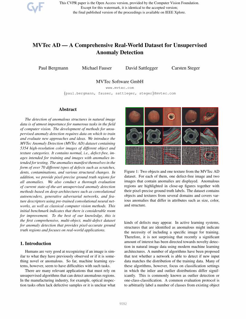
Figure 1: Two objects and one texture from the MVTec AD

dataset. For each of them, one defect-free image and two

images that contain anomalies are displayed. Anomalous

regions are highlighted in close-up figures together with

their pixel-precise ground truth labels. The dataset contains

objects and textures from several domains and covers var-

ious anomalies that differ in attributes such as size, color,

and structure.

kinds of defects may appear. In active learning systems,

structures that are identified as anomalous might indicate

the necessity of including a specific image for training.

Therefore, it is not surprising that recently a significant

amount of interest has been directed towards novelty detec-

tion in natural image data using modern machine learning

architectures. A number of algorithms have been proposed

that test whether a network is able to detect if new input

data matches the distribution of the training data. Many of

these algorithms, however, focus on classification settings

in which the inlier and outlier distributions differ signif-

icantly. This is commonly known as outlier detection or

one-class-classification. A common evaluation protocol is

to arbitrarily label a number of classes from existing object

9592

classification datasets as outlier classes and use the remain-

ing classes as inliers for training. It is then measured how

well the trained algorithm can distinguish between previ-

ously unseen outlier and inlier samples.

While this classification on an image level is important,

it is unclear how current state-of-the-art methods perform

on what we call anomaly detection tasks. The problem set-

ting is to find novelties in images that are very close to the

training data and differ only in subtle deviations in possibly

very small, confined regions. Clearly, to develop machine

learning models for such and other challenging scenarios

we require suitable data. Curiously, there is a lack of com-

prehensive real-world datasets available for such scenarios.

Large-scale datasets have led to incredible advances in

many areas of computer vision in the last few years. Just

consider how closely intertwined the development of new

classification methods is with the introduction of datasets

such as MNIST [16], CIFAR10 [14], or ImageNet [15].

To the best of our knowledge, no comparable dataset ex-

ists for the task of unsupervised anomaly detection. As a

first step to fill this gap and to spark further research in the

development of methods for unsupervised anomaly detec-

tion, we introduce the MVTec Anomaly Detection (MVTec

AD or MAD for short) dataset1 that facilitates a thorough

evaluation of such methods. We identify industrial inspec-

tion tasks as an ideal and challenging real-world use-case

for these scenarios. Defect-free example images of objects

or textures are used to train a model that must determine

whether an anomaly is present during test time. Unsuper-

vised methods play a significant role here since it is of-

ten unknown beforehand what types of defects might occur

during manufacturing. In addition, industrial processes are

optimized to produce a minimum amount of defective sam-

ples. Therefore, only a very limited amount of images with

defects is available, in contrast to a vast amount of defect-

free samples that can be used for training. Ideally, methods

should provide a pixel-accurate segmentation of anomalous

regions. All this makes industrial inspection tasks perfect

benchmarks for unsupervised anomaly detection methods

that work on natural images. Our contribution is twofold:

• We introduce a novel and comprehensive dataset for

the task of unsupervised anomaly detection in natu-

ral image data. It mimics real-world industrial inspec-

tion scenarios and consists of 5354 high-resolution im-

ages of five unique textures and ten unique objects

from different domains. There are 73 different types

of anomalies in the form of defects in the objects or

textures. For each defect image, we provide pixel-

accurate ground truth regions (1888 in total) that allow

to evaluate methods for both one-class classification

and anomaly detection.

1www.mvtec.com/company/research/datasets

• We conduct a thorough evaluation of current state-of-

the-art methods as well as more traditional methods for

unsupervised anomaly detection on the dataset. Their

performance for both segmentation and classification

of anomalous images is assessed. Furthermore, we

provide a well-defined way to detect anomalous re-

gions in test images using hyperparameters that are es-

timated without the knowledge of any anomalous im-

ages. We show that the evaluated methods do not per-

form equally well across object and defect categories

and that there is considerable room for improvement.

2. Related Work

2.1. Existing Datasets for Anomaly Detection

We first give a brief overview of datasets that are com-

monly used for anomaly detection in natural images and

demonstrate the need for our novel dataset. We distinguish

between datasets where a simple binary decision between

defect and defect-free images must be made and datasets

that allow for the segmentation of anomalous regions.

2.1.1 Classification of Anomalous Images

When evaluating methods for outlier detection in mutli-

class classification scenarios, a common practice is to adapt

existing classification datasets for which class labels are al-

ready available. The most prominent examples are MNIST

[16], CIFAR10 [14], and ImageNet [15]. A popular ap-

proach [1, 7, 21] is to select an arbitrary subset of classes,

re-label them as outliers, and train a novelty detection sys-

tem solely on the remaining inlier classes. During the test-

ing phase, it is checked whether the trained model is able

to correctly predict whether a test sample belongs to one of

the inliner classes. While this immediately provides a large

amount of training and testing data, the anomalous samples

differ significantly from the samples drawn from the train-

ing distribution. Therefore, when performing evaluations

on such datasets, it is unclear how a proposed method would

generalize to data where anomalies manifest themselves in

less significant differences from the training data manifold.

For this purpose, Saleh et al. [22] propose a dataset that

contains six categories of abnormally shaped objects, such

as oddly shaped cars, airplanes, and boats, obtained from in-

ternet search engines that should be distinguished from reg-

ular samples of the same class in the PASCAL VOC dataset

[8]. While their data might be closer to the training data

manifold, the decision is again based on entire images rather

than finding the parts of the images that make them novel or

anomalous.

9593

2.1.2 Segmentation of Anomalous Regions

For the evaluation of methods that segment anomalies in

images, only very few public datasets are currently avail-

able. All of them focus on the inspection of textured sur-

faces and, to the best of our knowledge, there does not yet

exist a comprehensive dataset that allows for the segmenta-

tion of anomalous regions in natural images.

Carrera et al. [6] provide NanoTWICE,2 a dataset of

45 gray-scale images that show a nanofibrous material ac-

quired by a scanning electron microscope. Five defect-free

images can be used for training. The remaining 40 images

contain anomalous regions in the form of specks of dust or

flattened areas. Since the dataset only provides a single kind

of texture, it is unclear how well algorithms that are evalu-

ated on this dataset generalize to other textures of different

domains.

A dataset that is specifically designed for optical in-

spection of textured surfaces was proposed during a 2007

DAGM workshop by Wieler and Hahn [28]. They provide

ten classes of artificially generated gray-scale textures with

defects weakly annotated in the form of ellipses. Each class

comprises 1000 defect-free texture patches for training and

150 defective patches for testing. However, their annota-

tions are quite coarse and since the textures were generated

by very similar texture models, the variance in appearance

between the different textures is quite low. Furthermore, ar-

tificially generated datasets can only be seen as an approxi-

mation to the real world.

2.2. Methods

The landscape of methods for unsupervised anomaly de-

tection is diverse and many approaches have been suggested

to tackle the problem [1, 19]. Pimentel et al. [20] give a

comprehensive review of existing work. We restrict our-

selves to a brief overview of current state-of-the art meth-

ods, focusing on those that serve as baseline for our initial

benchmark on the dataset.

2.2.1 Generative Adversarial Networks

Schlegl et al. [23] propose to model the manifold of the

training data by a generative adversarial network (GAN)

[10] that is trained solely on defect-free images. The gener-

ator is able to produce realistically looking images that fool

a simultaneously trained discriminator network in an adver-

sarial way. For anomaly detection, the algorithm searches

for a latent sample that reproduces a given input image and

manages to fool the discriminator. An anomaly segmenta-

tion can be obtained by a per-pixel comparison of the recon-

structed image with the original input.

2www.mi.imati.cnr.it/ettore/NanoTWICE/

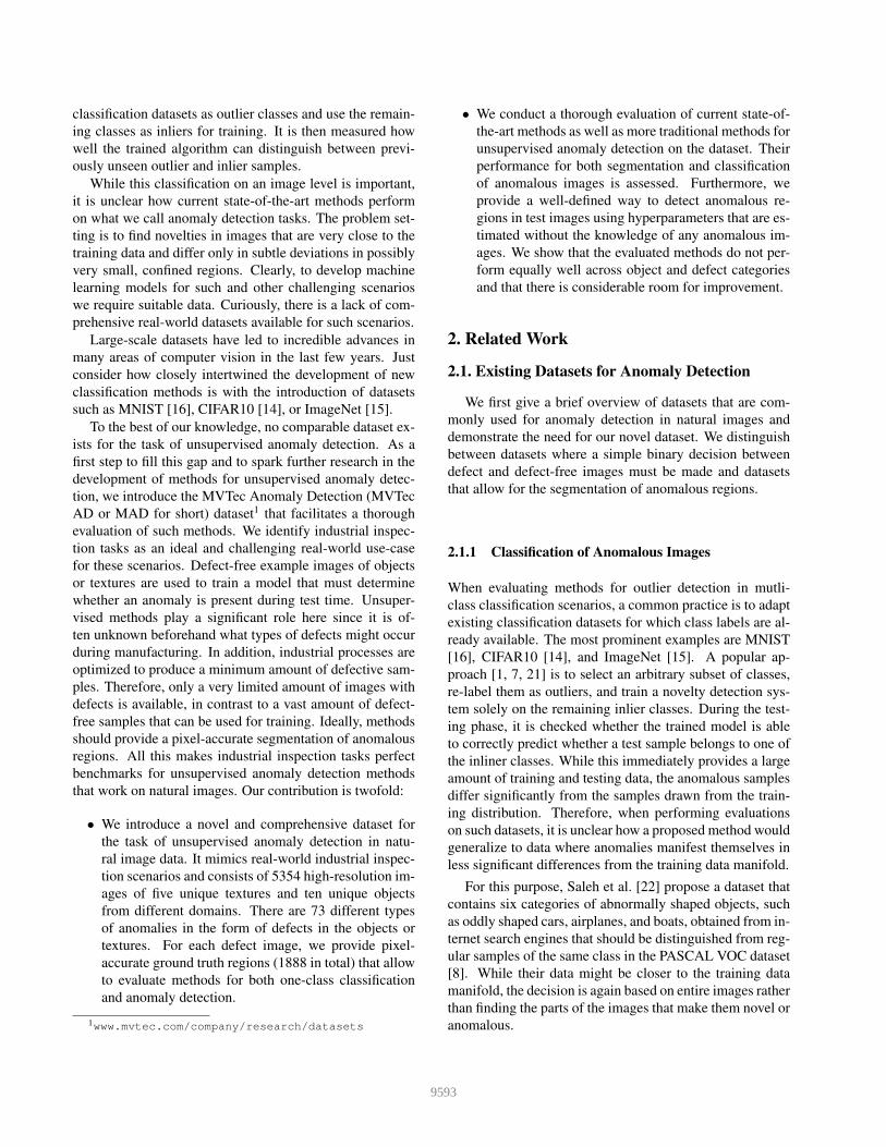
Figure 2: Example images for all five textures and ten ob-

ject categories of the MVTec AD dataset. For each cate-

gory, the top row shows an anomaly-free image. The middle

row shows an anomalous example for which, in the bottom

row, a close-up view that highlights the anomalous region is

given.

2.2.2 Deep Convolutional Autoencoders

Convolutional Autoencoders (CAEs) [9] are commonly

used as a base architecture in unsupervised anomaly detec-

tion settings. They attempt to reconstruct defect-free train-

ing samples through a bottleneck (latent space). During

testing, they fail to reproduce images that differ from the

data that was observed during training. Anomalies are de-

9594

Category # Train# Test

(good)

# Test

(defective)

# Defect

groups

# Defect

regions

Image

side length

Tex

ture

s

Carpet 280 28 89 5 97 1024

Grid 264 21 57 5 170 1024

Leather 245 32 92 5 99 1024

Tile 230 33 84 5 86 840

Wood 247 19 60 5 168 1024

Ob

ject

s

Bottle 209 20 63 3 68 900

Cable 224 58 92 8 151 1024

Capsule 219 23 109 5 114 1000

Hazelnut 391 40 70 4 136 1024

Metal Nut 220 22 93 4 132 700

Pill 267 26 141 7 245 800

Screw 320 41 119 5 135 1024

Toothbrush 60 12 30 1 66 1024

Transistor 213 60 40 4 44 1024

Zipper 240 32 119 7 177 1024

Total 3629 467 1258 73 1888 -

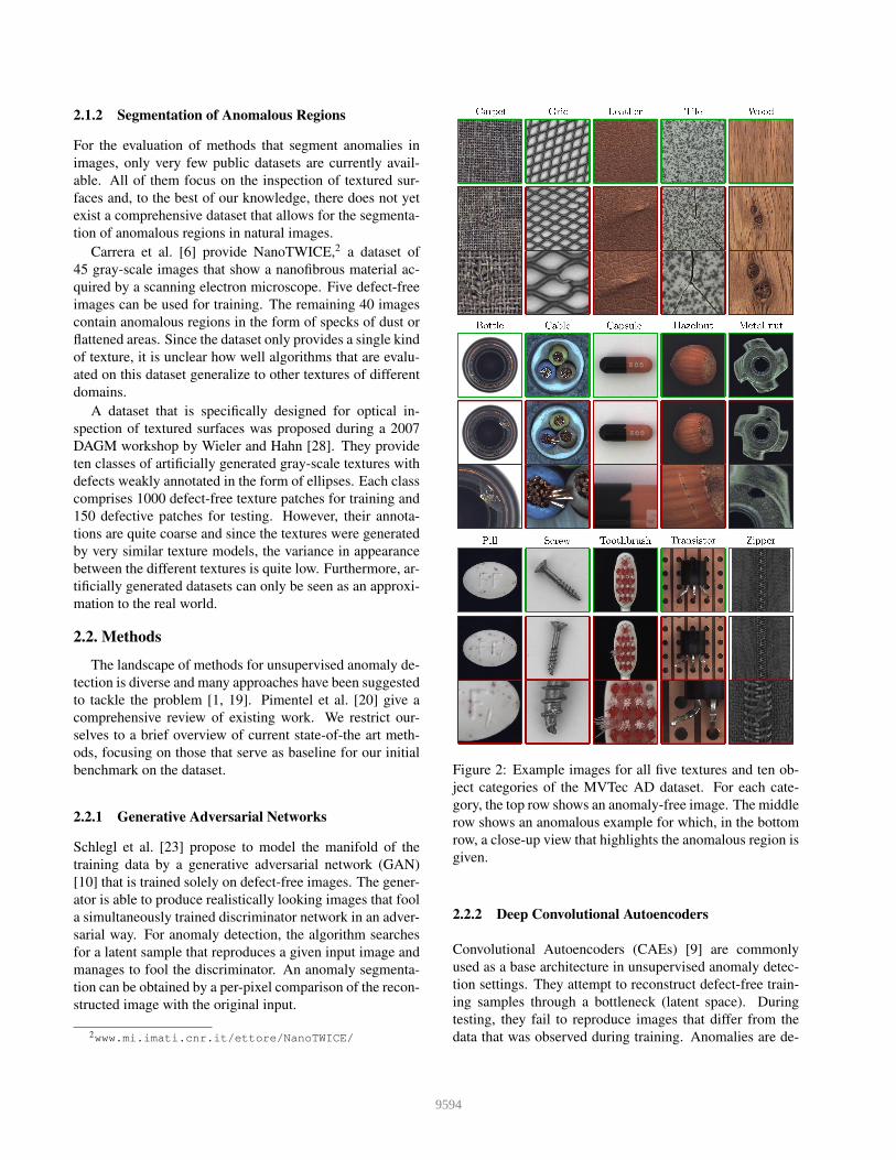
Table 1: Statistical overview of the MVTec AD dataset. For

each category, the number of training and test images is

given together with additional information about the defects

present in the respective test images.

tected by a per-pixel comparison of the input with its re-

construction. Recently, Bergmann et al. [4] pointed out the

disadvantages of per-pixel loss functions in autoencoding

frameworks when used in anomaly segmentation scenar-

ios and proposed to incorporate spatial information of local

patch regions using structural similarity [27] for improved

segmentation results.

There exist various extensions to CAEs such as the vari-

ational autoencoders (VAEs) [13] that have been used by

Baur et al. [3] for the unsupervised segmentation of anoma-

lies in brain MR scans. Baur et al., however, do not report

significant improvements over using standard CAEs. This

coincides with the observations made by Bergmann et al.

[4]. Nalisnick et al. [17] and Hendrycks et al. [12] provide

further evidence that probabilities obtained from VAEs and

other deep generative models might fail to model the true

likelihood of the training data. Therefore, we restrict our-

selves to deterministic autoencoder frameworks in the ini-

tial evaluation of the dataset below.

2.2.3 Features of Pre-trained Convolutional Neural

Networks

The aforementioned approaches attempt to learn feature

representations solely from the provided training data. In

addition, there exist a number of methods that use feature

descriptors obtained from CNNs that have been pre-trained

on a separate image classification task.

Napoletano et al. [18] propose to use clustered feature

descriptions obtained from the activations of a ResNet-18

[11] classification network pre-trained on ImageNet [15]

to distinguish normal from anomalous data. They achieve

state-of-the-art results on the NanoTWICE dataset. Being

designed for one-class classification, their method only pro-

vides a binary decision whether an input image contains an

anomaly or not. In order to obtain a spatial anomaly map,

the classifier must be evaluated at multiple image locations,

ideally at each single pixel. This quickly becomes a per-

formance bottleneck for large images. To increase perfor-

mance in practice, not every pixel location is evaluated and

the resulting anomaly maps are coarse.

2.2.4 Traditional Methods

In addition to the methods described above, we consider two

traditional methods for our benchmark. Bottger and Ulrich

[5] extract hand-crafted feature descriptors from defect-free

texture images. The distribution of feature vectors is mod-

eled by a Gaussian Mixture Model (GMM) and anomalies

are detected for extracted feature descriptors for which the

GMM yields a low probability. Their algorithm can only be

applied to images of regular textures.

In order to obtain a simple baseline for the non-texture

objects in the dataset, we consider the variation model [26,

Chapter 3.4.1.4]. This method requires a prior alignment

of the object contours and calculates the mean and standard

deviation for each pixel. This models the gray-value statis-

tics of the training images. During testing, a statistical test is

performed for each image pixel that measures the deviation

of the pixel’s gray-value from the mean. If the deviation is

larger than a threshold, an anomalous pixel is detected.

3. Dataset Description

The MVTec Anomaly Detection dataset comprises 15

categories with 3629 images for training and validation and

1725 images for testing. The training set contains only im-

ages without defects. The test set contains both: images

containing various types of defects and defect-free images.

Table 1 gives an overview for each object category. Some

example images for every category together with an ex-

ample defect are shown in Figure 2. We provide further

example images of the dataset in the supplementary mate-

rial. Five categories cover different types of regular (car-

pet, grid) or random (leather, tile, wood) textures, while

the remaining ten categories represent various types of ob-

jects. Some of these objects are rigid with a fixed appear-

ance (bottle, metal nut), while others are deformable (cable)

or include natural variations (hazelnut). A subset of objects

was acquired in a roughly aligned pose (e.g., toothbrush,

capsule, and pill) while others were placed in front of the

camera with a random rotation (e.g., metal nut, screw, and

hazelnut). The test images of anomalous samples contain

a variety of defects, such as defects on the objects’ surface

(e.g., scratches, dents), structural defects like distorted ob-

ject parts, or defects that manifest themselves by the ab-

sence of certain object parts. In total, 73 different defect

types are present, on average five per category. The defects

were manually generated with the aim to produce realistic

9595

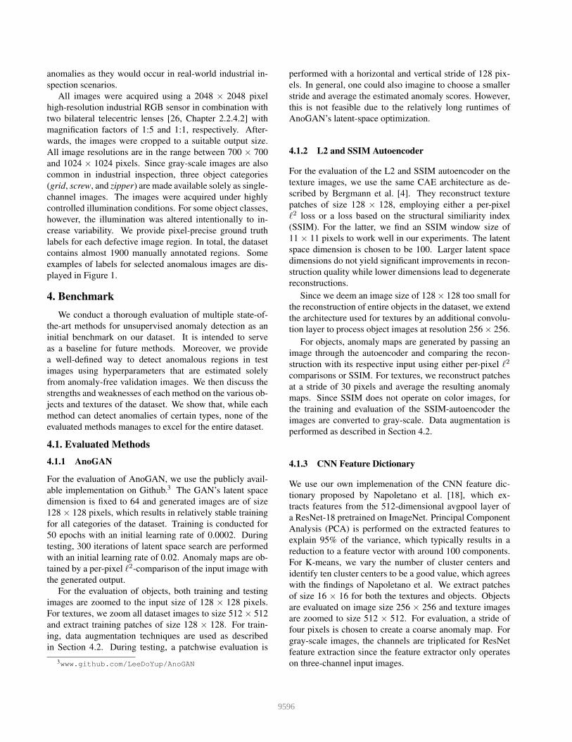
anomalies as they would occur in real-world industrial in-

spection scenarios.

All images were acquired using a 2048 × 2048 pixel

high-resolution industrial RGB sensor in combination with

two bilateral telecentric lenses [26, Chapter 2.2.4.2] with

magnification factors of 1:5 and 1:1, respectively. After-

wards, the images were cropped to a suitable output size.

All image resolutions are in the range between 700 × 700

and 1024 × 1024 pixels. Since gray-scale images are also

common in industrial inspection, three object categories

(grid, screw, and zipper) are made available solely as single-

channel images. The images were acquired under highly

controlled illumination conditions. For some object classes,

however, the illumination was altered intentionally to in-

crease variability. We provide pixel-precise ground truth

labels for each defective image region. In total, the dataset

contains almost 1900 manually annotated regions. Some

examples of labels for selected anomalous images are dis-

played in Figure 1.

4. Benchmark

We conduct a thorough evaluation of multiple state-of-

the-art methods for unsupervised anomaly detection as an

initial benchmark on our dataset. It is intended to serve

as a baseline for future methods. Moreover, we provide

a well-defined way to detect anomalous regions in test

images using hyperparameters that are estimated solely

from anomaly-free validation images. We then discuss the

strengths and weaknesses of each method on the various ob-

jects and textures of the dataset. We show that, while each

method can detect anomalies of certain types, none of the

evaluated methods manages to excel for the entire dataset.

4.1. Evaluated Methods

4.1.1 AnoGAN

For the evaluation of AnoGAN, we use the publicly avail-

able implementation on Github.3 The GAN’s latent space

dimension is fixed to 64 and generated images are of size

128 × 128 pixels, which results in relatively stable training

for all categories of the dataset. Training is conducted for

50 epochs with an initial learning rate of 0.0002. During

testing, 300 iterations of latent space search are performed

with an initial learning rate of 0.02. Anomaly maps are ob-

tained by a per-pixel ℓ2-comparison of the input image with

the generated output.

For the evaluation of objects, both training and testing

images are zoomed to the input size of 128 × 128 pixels.

For textures, we zoom all dataset images to size 512 × 512

and extract training patches of size 128 × 128. For train-

ing, data augmentation techniques are used as described

in Section 4.2. During testing, a patchwise evaluation is

3www.github.com/LeeDoYup/AnoGAN

performed with a horizontal and vertical stride of 128 pix-

els. In general, one could also imagine to choose a smaller

stride and average the estimated anomaly scores. However,

this is not feasible due to the relatively long runtimes of

AnoGAN’s latent-space optimization.

4.1.2 L2 and SSIM Autoencoder

For the evaluation of the L2 and SSIM autoencoder on the

texture images, we use the same CAE architecture as de-

scribed by Bergmann et al. [4]. They reconstruct texture

patches of size 128 × 128, employing either a per-pixel

ℓ2 loss or a loss based on the structural similiarity index

(SSIM). For the latter, we find an SSIM window size of

11 × 11 pixels to work well in our experiments. The latent

space dimension is chosen to be 100. Larger latent space

dimensions do not yield significant improvements in recon-

struction quality while lower dimensions lead to degenerate

reconstructions.

Since we deem an image size of 128 × 128 too small for

the reconstruction of entire objects in the dataset, we extend

the architecture used for textures by an additional convolu-

tion layer to process object images at resolution 256 × 256.

For objects, anomaly maps are generated by passing an

image through the autoencoder and comparing the recon-

struction with its respective input using either per-pixel ℓ2

comparisons or SSIM. For textures, we reconstruct patches

at a stride of 30 pixels and average the resulting anomaly

maps. Since SSIM does not operate on color images, for

the training and evaluation of the SSIM-autoencoder the

images are converted to gray-scale. Data augmentation is

performed as described in Section 4.2.

4.1.3 CNN Feature Dictionary

We use our own implemenation of the CNN feature dic-

tionary proposed by Napoletano et al. [18], which ex-

tracts features from the 512-dimensional avgpool layer of

a ResNet-18 pretrained on ImageNet. Principal Component

Analysis (PCA) is performed on the extracted features to

explain 95% of the variance, which typically results in a

reduction to a feature vector with around 100 components.

For K-means, we vary the number of cluster centers and

identify ten cluster centers to be a good value, which agrees

with the findings of Napoletano et al. We extract patches

of size 16 × 16 for both the textures and objects. Objects

are evaluated on image size 256 × 256 and texture images

are zoomed to size 512 × 512. For evaluation, a stride of

four pixels is chosen to create a coarse anomaly map. For

gray-scale images, the channels are triplicated for ResNet

feature extraction since the feature extractor only operates

on three-channel input images.

9596

CategoryAE

(SSIM)

AE

(L2)AnoGAN

CNN

Feature

Dictionary

Texture

Inspection

Variation

Model

Tex

ture

s

Carpet0.43

0.90

0.57

0.42

0.82

0.16

0.89

0.36

0.57

0.61-

Grid0.38

1.00

0.57

0.98

0.90

0.12

0.57

0.33

1.00

0.05-

Leather0.00

0.92

0.06

0.82

0.91

0.12

0.63

0.71

0.00

0.99-

Tile1.00

0.04

1.00

0.54

0.97

0.05

0.97

0.44

1.00

0.43-

Wood0.84

0.82

1.00

0.47

0.89

0.47

0.79

0.88

0.42

1.00-

Obje

cts

Bottle0.85

0.90

0.70

0.89

0.95

0.43

1.00

0.06-

1.00

0.13

Cable0.74

0.48

0.93

0.18

0.98

0.07

0.97

0.24- -

Capsule0.78

0.43

1.00

0.24

0.96

0.20

0.78

0.03-

1.00

0.03

Hazelnut1.00

0.07

0.93

0.84

0.83

0.16

0.90

0.07- -

Metal nut1.00

0.08

0.68

0.77

0.86

0.13

0.55

0.74-

0.32

0.83

Pill0.92

0.28

1.00

0.23

1.00

0.24

0.85

0.06-

1.00

0.13

Screw0.95

0.06

0.98

0.39

0.41

0.28

0.73

0.13-

1.00

0.10

Toothbrush0.75

0.73

1.00

0.97

1.00

0.13

1.00

0.03-

1.00

0.60

Transistor1.00

0.03

0.97

0.45

0.98

0.35

1.00

0.15- -

Zipper1.00

0.60

0.97

0.63

0.78

0.40

0.78

0.29- -

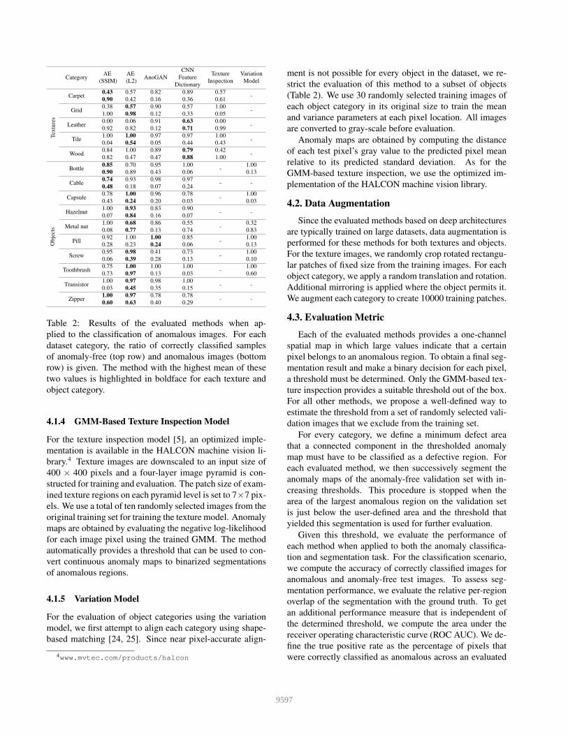
Table 2: Results of the evaluated methods when ap-

plied to the classification of anomalous images. For each

dataset category, the ratio of correctly classified samples

of anomaly-free (top row) and anomalous images (bottom

row) is given. The method with the highest mean of these

two values is highlighted in boldface for each texture and

object category.

4.1.4 GMM-Based Texture Inspection Model

For the texture inspection model [5], an optimized imple-

mentation is available in the HALCON machine vision li-

brary.4 Texture images are downscaled to an input size of

400 × 400 pixels and a four-layer image pyramid is con-

structed for training and evaluation. The patch size of exam-

ined texture regions on each pyramid level is set to 7×7 pix-

els. We use a total of ten randomly selected images from the

original training set for training the texture model. Anomaly

maps are obtained by evaluating the negative log-likelihood

for each image pixel using the trained GMM. The method

automatically provides a threshold that can be used to con-

vert continuous anomaly maps to binarized segmentations

of anomalous regions.

4.1.5 Variation Model

For the evaluation of object categories using the variation

model, we first attempt to align each category using shape-

based matching [24, 25]. Since near pixel-accurate align-

4www.mvtec.com/products/halcon

ment is not possible for every object in the dataset, we re-

strict the evaluation of this method to a subset of objects

(Table 2). We use 30 randomly selected training images of

each object category in its original size to train the mean

and variance parameters at each pixel location. All images

are converted to gray-scale before evaluation.

Anomaly maps are obtained by computing the distance

of each test pixel’s gray value to the predicted pixel mean

relative to its predicted standard deviation. As for the

GMM-based texture inspection, we use the optimized im-

plementation of the HALCON machine vision library.

4.2. Data Augmentation

Since the evaluated methods based on deep architectures

are typically trained on large datasets, data augmentation is

performed for these methods for both textures and objects.

For the texture images, we randomly crop rotated rectangu-

lar patches of fixed size from the training images. For each

object category, we apply a random translation and rotation.

Additional mirroring is applied where the object permits it.

We augment each category to create 10000 training patches.

4.3. Evaluation Metric

Each of the evaluated methods provides a one-channel

spatial map in which large values indicate that a certain

pixel belongs to an anomalous region. To obtain a final seg-

mentation result and make a binary decision for each pixel,

a threshold must be determined. Only the GMM-based tex-

ture inspection provides a suitable threshold out of the box.

For all other methods, we propose a well-defined way to

estimate the threshold from a set of randomly selected vali-

dation images that we exclude from the training set.

For every category, we define a minimum defect area

that a connected component in the thresholded anomaly

map must have to be classified as a defective region. For

each evaluated method, we then successively segment the

anomaly maps of the anomaly-free validation set with in-

creasing thresholds. This procedure is stopped when the

area of the largest anomalous region on the validation set

is just below the user-defined area and the threshold that

yielded this segmentation is used for further evaluation.

Given this threshold, we evaluate the performance of

each method when applied to both the anomaly classifica-

tion and segmentation task. For the classification scenario,

we compute the accuracy of correctly classified images for

anomalous and anomaly-free test images. To assess seg-

mentation performance, we evaluate the relative per-region

overlap of the segmentation with the ground truth. To get

an additional performance measure that is independent of

the determined threshold, we compute the area under the

receiver operating characteristic curve (ROC AUC). We de-

fine the true positive rate as the percentage of pixels that

were correctly classified as anomalous across an evaluated

9597

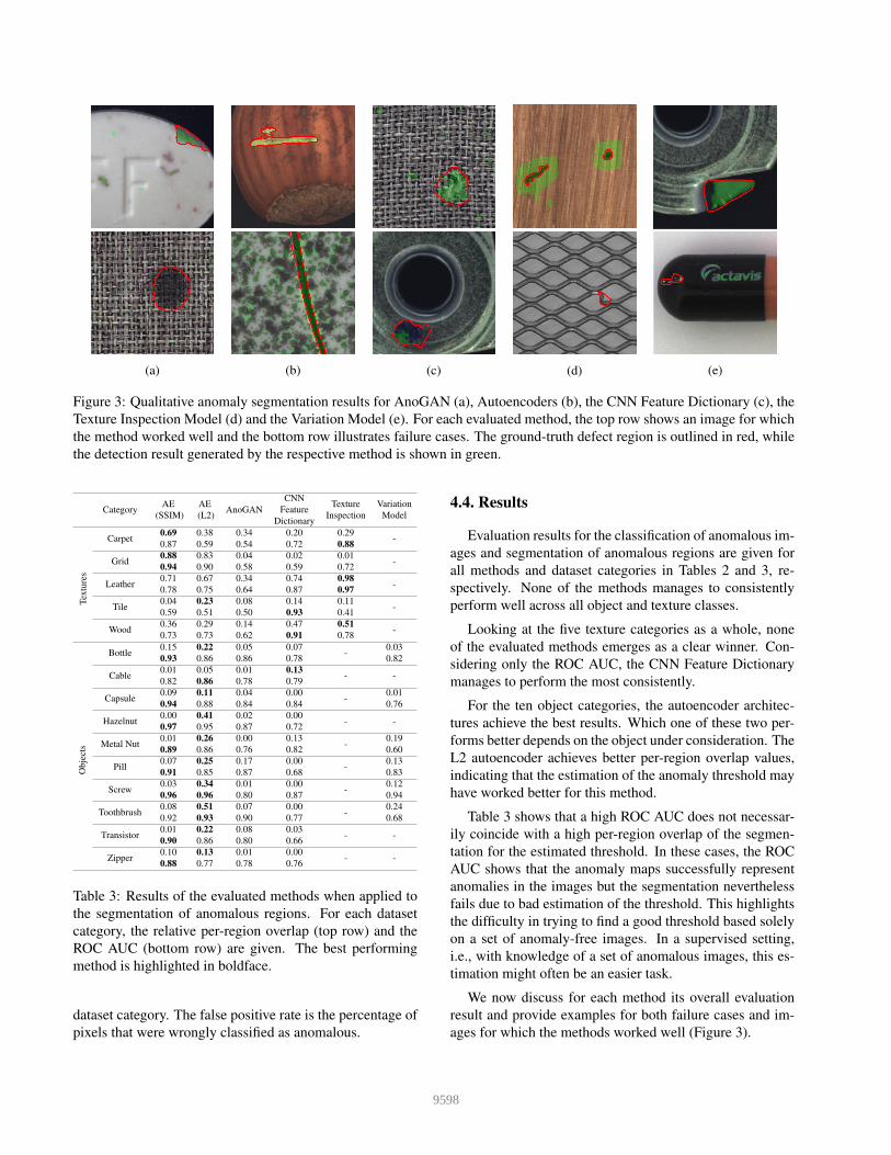
(a) (b) (c) (d) (e)

Figure 3: Qualitative anomaly segmentation results for AnoGAN (a), Autoencoders (b), the CNN Feature Dictionary (c), the

Texture Inspection Model (d) and the Variation Model (e). For each evaluated method, the top row shows an image for which

the method worked well and the bottom row illustrates failure cases. The ground-truth defect region is outlined in red, while

the detection result generated by the respective method is shown in green.

CategoryAE

(SSIM)

AE

(L2)AnoGAN

CNN

Feature

Dictionary

Texture

Inspection

Variation

Model

Tex

ture

s

Carpet0.69

0.87

0.38

0.59

0.34

0.54

0.20

0.72

0.29

0.88-

Grid0.88

0.94

0.83

0.90

0.04

0.58

0.02

0.59

0.01

0.72-

Leather0.71

0.78

0.67

0.75

0.34

0.64

0.74

0.87

0.98

0.97-

Tile0.04

0.59

0.23

0.51

0.08

0.50

0.14

0.93

0.11

0.41-

Wood0.36

0.73

0.29

0.73

0.14

0.62

0.47

0.91

0.51

0.78-

Obje

cts

Bottle0.15

0.93

0.22

0.86

0.05

0.86

0.07

0.78-

0.03

0.82

Cable0.01

0.82

0.05

0.86

0.01

0.78

0.13

0.79- -

Capsule0.09

0.94

0.11

0.88

0.04

0.84

0.00

0.84-

0.01

0.76

Hazelnut0.00

0.97

0.41

0.95

0.02

0.87

0.00

0.72- -

Metal Nut0.01

0.89

0.26

0.86

0.00

0.76

0.13

0.82-

0.19

0.60

Pill0.07

0.91

0.25

0.85

0.17

0.87

0.00

0.68-

0.13

0.83

Screw0.03

0.96

0.34

0.96

0.01

0.80

0.00

0.87-

0.12

0.94

Toothbrush0.08

0.92

0.51

0.93

0.07

0.90

0.00

0.77-

0.24

0.68

Transistor0.01

0.90

0.22

0.86

0.08

0.80

0.03

0.66- -

Zipper0.10

0.88

0.13

0.77

0.01

0.78

0.00

0.76- -

Table 3: Results of the evaluated methods when applied to

the segmentation of anomalous regions. For each dataset

category, the relative per-region overlap (top row) and the

ROC AUC (bottom row) are given. The best performing

method is highlighted in boldface.

dataset category. The false positive rate is the percentage of

pixels that were wrongly classified as anomalous.

4.4. Results

Evaluation results for the classification of anomalous im-

ages and segmentation of anomalous regions are given for

all methods and dataset categories in Tables 2 and 3, re-

spectively. None of the methods manages to consistently

perform well across all object and texture classes.

Looking at the five texture categories as a whole, none

of the evaluated methods emerges as a clear winner. Con-

sidering only the ROC AUC, the CNN Feature Dictionary

manages to perform the most consistently.

For the ten object categories, the autoencoder architec-

tures achieve the best results. Which one of these two per-

forms better depends on the object under consideration. The

L2 autoencoder achieves better per-region overlap values,

indicating that the estimation of the anomaly threshold may

have worked better for this method.

Table 3 shows that a high ROC AUC does not necessar-

ily coincide with a high per-region overlap of the segmen-

tation for the estimated threshold. In these cases, the ROC

AUC shows that the anomaly maps successfully represent

anomalies in the images but the segmentation nevertheless

fails due to bad estimation of the threshold. This highlights

the difficulty in trying to find a good threshold based solely

on a set of anomaly-free images. In a supervised setting,

i.e., with knowledge of a set of anomalous images, this es-

timation might often be an easier task.

We now discuss for each method its overall evaluation

result and provide examples for both failure cases and im-

ages for which the methods worked well (Figure 3).

9598

4.4.1 AnoGAN

We observe a tendency of GAN training to result in mode

collapse [2]. The generator then often completely fails to

reproduce a given test image since all latent samples gen-

erate more or less the same image. As a consequence,

AnoGAN has great difficulties with object categories for

which the objects appear in various shapes or orientations

in the dataset. It performs better for object categories that

contain less variations, such as bottle and pill. This can be

seen in Figure 3a, where AnoGAN manages to detect the

crack on the pill. However, it fails to generate small de-

tails on the pill such as the colored speckles, which it also

detects as anomalies. For the category carpet, AnoGAN is

unable to model all the subtle variations of the textural pat-

tern, which results in a complete failure of the method as

can be seen in the bottom row of Figure 3a.

4.4.2 L2 and SSIM Autoencoder

We observe stable training across all dataset categories

with reasonable reconstructions for both the SSIM and L2

autoencoder. Especially for the object categories of the

dataset, both autoencoders outperform all other evaluated

methods in the majority of cases. For some categories, how-

ever, both autoencoders fail to model small details, which

results in rather blurry image reconstructions. This is es-

pecially the case for high-frequency textures, which appear,

for example, in tile and zipper. The bottom row of Fig-

ure 3b shows that for tile, the L2 autoencoder, in addition

to the cracked surface, detects many false positive regions

across the entire image. A similar behavior can be observed

for the SSIM autoencoder.

4.4.3 CNN Feature Dictionary

As a method proposed for the detection of anomalous re-

gions in textured surfaces, the feature dictionary based on

CNN features achieves satisfactory results for all textures

except grid. Since it does not incorporate additional in-

formation about the spatial location of the extracted fea-

tures, its performance degenerates when evaluated on ob-

jects. Figure 3c demonstrates good anomaly segmentation

performance for carpet with only few false positives, while

the color defect on metal nut is only partially found.

4.4.4 GMM-Based Texture Inspection Model

Specifically designed to operate on texture images, the

GMM-based texture inspection model performs well across

most texture categories of the dataset. On grid, however,

it cannot achieve satisfactory results due to many small de-

fects for which its sensitivity is not high enough (Figure 3d).

Furthermore, since it only operates on gray-scale images, it

fails to detect most color-based defects.

4.4.5 Variation Model

For the variation model, good performance can be observed

on screw, toothbrush, and bottle, while it yields compara-

bly bad results for metal nut and capsule. This is mostly

due to the fact that the latter objects contain certain random

variations on the objects’ surfaces, which prevents the vari-

ation model from learning reasonable mean and variance

values for most of the image pixels. Figure 3e illustrates

this behavior: since the imprint on the capsule can appear at

various locations, it will always be misclassified as a defect.

5. Conclusions

We introduce the MVTec Anomaly Detection dataset, a

novel dataset for unsupervised anomaly detection mimick-

ing real-world industrial inspection scenarios. The dataset

provides the possibility to evaluate unsupervised anomaly

detection methods on various texture and object classes with

different types of anomalies. Because pixel-precise ground

truth labels for anomalous regions in the images are pro-

vided, it is possible to evaluate anomaly detection methods

for both image-level classification as well as pixel-level seg-

mentation.

Several state-of-the-art methods as well as two classi-

cal methods were thoroughly evaluated on this dataset. The

evaluations provide a first benchmark on this dataset and

show that there is still considerable room for improvement.

It is our hope that the proposed dataset will stimulate the

development of new unsupervised anomaly detection meth-

ods.

References

[1] J. An and S. Cho. Variational Autoencoder based Anomaly

Detection using Reconstruction Probability. Technical re-

port, SNU Data Mining Center, 2015.

[2] M. Arjovsky and L. Bottou. Towards Principled Methods

for Training Generative Adversarial Networks. International

Conference on Learning Representations, 2017.

[3] C. Baur, B. Wiestler, S. Albarqouni, and N. Navab. Deep

Autoencoding Models for Unsupervised Anomaly Segmen-

tation in Brain MR Images. In A. Crimi, S. Bakas, H. Kuijf,

F. Keyvan, M. Reyes, and T. van Walsum, editors, Brain-

lesion: Glioma, Multiple Sclerosis, Stroke and Traumatic

Brain Injuries, pages 161–169, Cham, 2019. Springer Inter-

national Publishing.

[4] P. Bergmann, S. Lowe, M. Fauser, D. Sattlegger, and C. Ste-

ger. Improving Unsupervised Defect Segmentation by Ap-

plying Structural Similarity to Autoencoders. In A. Tremeau,

G. Farinella, and J. Braz, editors, 14th International Joint

Conference on Computer Vision, Imaging and Computer

9599

Graphics Theory and Applications, volume 5: VISAPP,

pages 372–380, Setubal, 2019. Scitepress.

[5] T. Bottger and M. Ulrich. Real-time Texture Error Detec-

tion on Textured Surfaces with Compressed Sensing. Pattern

Recognition and Image Analysis, 26(1):88–94, 2016.

[6] D. Carrera, F. Manganini, G. Boracchi, and E. Lanzarone.

Defect Detection in SEM Images of Nanofibrous Materi-

als. IEEE Transactions on Industrial Informatics, 13(2):551–

561, 2017.

[7] R. Chalapathy, A. K. Menon, and S. Chawla. Anomaly De-

tection using One-Class Neural Networks. arXiv preprint

arXiv:1802.06360, 2018.

[8] M. Everingham, S. M. A. Eslami, L. Van Gool, C. K. I.

Williams, J. Winn, and A. Zisserman. The Pascal Visual

Object Classes Challenge: A Retrospective. International

Journal of Computer Vision, 111(1):98–136, Jan. 2015.

[9] I. Goodfellow, Y. Bengio, and A. Courville. Deep Learning.

MIT Press, Cambridge, MA, 2016.

[10] I. Goodfellow, J. Pouget-Abadie, M. Mirza, B. Xu,

D. Warde-Farley, S. Ozair, A. Courville, and Y. Bengio. Gen-

erative Adversarial Nets. In Advances in Neural Information

Processing Systems, pages 2672–2680, 2014.

[11] K. He, X. Zhang, S. Ren, and J. Sun. Deep Residual Learning

for Image Recognition. In IEEE Conference on Computer

Vision and Pattern Recognition, pages 770–778, 2016.

[12] D. Hendrycks, M. Mazeika, and T. Dietterich. Deep

Anomaly Detection with Outlier Exposure. Proceedings of

the International Conference on Learning Representations,

2019.

[13] D. P. Kingma and M. Welling. Auto-Encoding Variational

Bayes. International Conference on Learning Representa-

tions, 2014.

[14] A. Krizhevsky and G. Hinton. Learning multiple layers of

features from tiny images. Technical report, University of

Toronto, 2009.

[15] A. Krizhevsky, I. Sutskever, and G. E. Hinton. ImageNet

Classification with Deep Convolutional Neural Networks. In

Proceedings of the 25th International Conference on Neu-

ral Information Processing Systems - Volume 1, pages 1097–

1105, 2012.

[16] Y. LeCun, L. Bottou, Y. Bengio, and P. Haffner. Gradient-

based learning applied to document recognition. Proceed-

ings of the IEEE, 86(11):2278–2324, 1998.

[17] E. Nalisnick, A. Matsukawa, Y. W. Teh, D. Gorur, and

B. Lakshminarayanan. Do Deep Generative Models Know

What They Don’t Know? International Conference on

Learning Representations, 2019.

[18] P. Napoletano, F. Piccoli, and R. Schettini. Anomaly

Detection in Nanofibrous Materials by CNN-Based Self-

Similarity. Sensors, 18(1):209, 2018.

[19] P. Perera and V. M. Patel. Learning Deep Features for

One-Class Classification. arXiv preprint arXiv:1801.05365,

2018.

[20] M. A. Pimentel, D. A. Clifton, L. Clifton, and L. Tarassenko.

A review of novelty detection. Signal Processing, 99:215–

249, 2014.

[21] L. Ruff, R. Vandermeulen, N. Goernitz, L. Deecke, S. A. Sid-

diqui, A. Binder, E. Muller, and M. Kloft. Deep One-Class

Classification. In J. Dy and A. Krause, editors, Proceedings

of the 35th International Conference on Machine Learning,

volume 80 of Proceedings of Machine Learning Research,

pages 4393–4402. PMLR, 2018.

[22] B. Saleh, A. Farahdi, and A. Elgammal. Object-Centric

Anomaly Detection by Attribute-Based Reasoning. IEEE

Conference on Computer Vision and Pattern Recognition,

pages 787–794, 2013.

[23] T. Schlegl, P. Seebock, S. M. Waldstein, U. Schmidt-Erfurth,

and G. Langs. Unsupervised Anomaly Detection with Gen-

erative Adversarial Networks to Guide Marker Discovery. In

International Conference on Information Processing in Med-

ical Imaging, pages 146–157. Springer, 2017.

[24] C. Steger. Similarity Measures for Occlusion, Clutter, and

Illumination Invariant Object Recognition. In B. Radig and

S. Florczyk, editors, Pattern Recognition, volume 2191 of

Lecture Notes in Computer Science, pages 148–154, Berlin,

2001. Springer-Verlag.

[25] C. Steger. Occlusion, Clutter, and Illumination Invariant Ob-

ject Recognition. In International Archives of Photogram-

metry and Remote Sensing, volume XXXIV, part 3A, pages

345–350, 2002.

[26] C. Steger, M. Ulrich, and C. Wiedemann. Machine Vision

Algorithms and Applications. Wiley-VCH, Weinheim, 2nd

edition, 2018.

[27] Z. Wang, A. C. Bovik, H. R. Sheikh, and E. P. Simoncelli.

Image quality assessment: from error visibility to struc-

tural similarity. IEEE Transactions on Image Processing,

13(4):600–612, 2004.

[28] M. Wieler and T. Hahn. Weakly Supervised Learning

for Industrial Optical Inspection. Online: resources.mpi-

inf.mpg.de/conference/dagm/2007/prizes.html. Accessed

2018-11-16.

9600