musclenet: mapping electromyography to kinematic and

Pre-PRINT

MuscleNET: mapping electromyography tokinematic and dynamic biomechanical variables bymachine learning

Ali Nasr, Sydney Bell, Jiayuan He, Rachel L. Whittaker,Ning Jiang, Clark R. Dickerson, and John McPhee

University of Waterloo, Ontario N2L 1W2, Canada

E-mail: [email protected]

Abstract. Objective. This paper proposes machine learning models for mappingsurface electromyography (sEMG) signals to regression of joint angle, jointvelocity, joint acceleration, joint torque, and activation torque. Approach. Theregression models, collectively known as MuscleNET, take one of four forms:ANN (Forward Artificial Neural Network), RNN (Recurrent Neural Network),CNN (Convolutional Neural Network), and RCNN (Recurrent ConvolutionalNeural Network). Inspired by conventional biomechanical muscle models, delayedkinematic signals were used along with sEMG signals as the machine learningmodel’s input; specifically, the CNN and RCNN were modeled with novelconfigurations for these input conditions. The models’ inputs contain either rawor filtered sEMG signals, which allowed evaluation of the filtering capabilitiesof the models. The models were trained using human experimental data andevaluated with different individual data. Main results. Results were comparedin terms of regression error (using the root-mean-square) and model computationdelay. The results indicate that the RNN (with filtered sEMG signals) and RCNN(with raw sEMG signals) models, both with delayed kinematic data, can extractunderlying motor control information (such as joint activation torque or jointangle) from sEMG signals in pick-and-place tasks. The CNNs and RCNNs wereable to filter raw sEMG signals. Significance. All forms of MuscleNET were foundto map sEMG signals within 2 ms, fast enough for real-time applications such asthe control of exoskeletons or active prostheses. The RNN model with filteredsEMG and delayed kinematic signals is particularly appropriate for applicationsin musculoskeletal simulation and biomechatronic device control.

Machine learning model, Muscle model, Electromyography, Myoelectric signals,Myoelectric control, EMG-based control Submitted to: J. Neural Eng.

Pre-PRINT

MuscleNET: Mapping Electromyography to kinematic and dynamic biomechanical variables 2

1. Introduction

For volitional control, rehabilitation assessment, intentdetection, and power assist, biological signals are theprimary inputs of robotic prostheses, active exoskele-tons, human-computer interfaces, and rehabilitationrobots [1]. One of the primary bio-signals for motion-intention recognition is the electromyography (EMG)signal, which measures the electric potential differencetriggered by the nervous system to command musclecontraction [2]. Myoelectric control of biomechatronicdevices has encouraged the study of more advancedsEMG control algorithms [3]. Accordingly, two mainstrategies have been used: (a) detailed muscle model-ing and (b) machine learning methods.

One way to convert the sEMG signal to themuscle joint torque is to use a biomechanical musclemodel. The most commonly used model is thethree-component model, which takes inspiration fromthe lumped-parameter model developed by A.V. Hillfor active and passive muscle tension behavior [4].However, including a general muscle model withina multibody model introduces various shortcomingssuch as muscle redundancy, a need to specify complexmusculoskeletal geometry such as intricate musclewrapping pathways and, difficult-to-fit parameters foreach muscle, along with sensitivity to these additionalparameters. One method that alleviates the musclegeometry, complexity, redundancy, and interpretationof sEMG signals within a control framework uses amachine learning model trained by experimental data.

The output of the machine learning method canbe categorized into two groups: (A) a set of decisions,classes, or conditions [5–12], and (B) a data-drivenkinematic or kinetic prediction value (regression-based)[13, 14]. The set of classes is usually used for statecontrol and requires a large window of data to makethe precise prediction class. Specifically, classificationis a post-processing technique that requires the motiondata after the motion task is completed. Thus, theregression method has superiority over classificationmethod in terms of real-time processing. Theregression-based schemes provide the capability ofindependent, simultaneous, real-time, and volitionalcontrol of each degree of freedom (DoF).

From the general input perspective, the machinelearning models fall into two groups: (1) the singleinstantaneous value of the sEMG signal [15] and (2)pattern recognition techniques (discovering regularities

in the pattern of the data) [11,16–18] Due to the sEMGsignals’ stochastic and time-varying nature, sEMGsignal windows are utilized for pattern recognitioninstead of a single instantaneous value. The insufficientand stochastic nature of raw sEMG signals may besolved partially by using a considerable amount oftraining data and a complex machine learning model.

Transformation of a set or a window of sEMGdata into a more readily implemented decreased setof features often uses two methods: (1) featureengineering and (2) machine learning. Featureengineering method’s performance relies on the choiceof features for extracting discriminative informationfrom the sEMG data [9, 19–24]. Since the sEMGsignal contains temporal or spectral information, thelearning algorithms should not rely on specific andlimited features. On the other hand, the deep-learningsolution uses a hierarchy representation, which learnscomplex features by configuring and extracting stacksof features [25]. Deep learning architectures, likeRecurrent Neural Networks (RNN)s, ConvolutionalNeural Networks (CNN)s, and Recurrent CNNs(RCNN)s, are primarily used in image analysis orprocessing [26], speech recognition [27], and recently,bioinformatics [28].

Owing to the CNN’s broad feature learningcapability, they have become the most popular deeplearning architectures that can perform classificationor regression using multi-dimensional data [29]. Lately,CNNs have been applied in sEMG-based classificationof hand or wrist gestures [5, 6, 12, 17, 30, 31], andlimitedly in sEMG-based regression [32, 33]. Bao etal. [32] used a CNN for wrist multi-DoFs kinematicsestimation. Ameri et al. [34] introduced a regression-based CNN that was developed for real-time sEMGbased estimation of simultaneous wrist motions.

The RCNN is a particular type of CNN and canmine sequential data or time-frequency information.Chen et al. [13] used an RCNN as sEMG-to-Forcemapping for multi-DoFs finger force prediction. Theymade significant improvements to the predictionresults with an RCNN consisting of Long Short-TermMemory (LSTM) networks. Moreover, an RCNNhas been utilized for offline estimation of upper-limbmotions using sEMG frequency bands [35,36] and wristmotion intention recognition using the time-frequencyspectrum of sEMG signals [37].

The main similarity of the previous studies is thatthe estimators depend only on the sEMG signal as

Pre-PRINT


an input. However, by considering the biomechanicalmuscle model, the muscle tension relies on the joint’skinematics in addition to the sEMG signals thatfunction as an activation. The joint angle, velocity,and acceleration partially define the muscle’s tension,with the joint angle specifically defining the musclefiber orientation. The fiber orientation indicatesthe direction of tension applied on the bone, andconsequently the joint torque. Thus, we propose thatin addition to the sEMG signal, the joint’s kinematicsbe used as input signals to a machine learning model.

In summary, this work’s distinguishing character-istics and novelties are (1) regression-based mappingfor intent recognition, muscle modeling, and volitionalcontrol of biomechatronic devices, such as exoskeletons,prostheses, and assistive/resistive robots; (2) real-timemapping of sEMG signals by using an optimum num-ber of layers in the machine learning model; (3) propos-ing a novel structure of CNN and RCNN for filteringraw sEMG signals and feature learning of muscle dy-namics; and (4) using delayed joint kinematics as asecond input type, inspired by biomechanical musclemodels. The proposed MuscleNET (defined as the ma-chine learning models of sEMG signals to regression ofkinematic and dynamic biomechanical variables) hasseveral applications, including representing muscles ina musculoskeletal simulation, sports biomechanics sim-ulation, controlling active exoskeletons and prostheses,developing model-based assistive/resistive robots, andpost-rehabilitation analysis.

In this paper, firstly, the data preparation stepsare described. Secondly, the configuration of themachine learning models is introduced. Finally,the training results of 80 models are discussed andcompared.

2. Data Preparation

This section presents the data collection [38, 39] andprocessing methods. The data preparation steps havebeen visualized in Figure 1. The processed datawas used for training the machine learning models,as detailed in section 3. The data is available uponreasonable request from the corresponding author [38,39]. Due to ethical and privacy restrictions, the datais not publicly available.

2.1. Subjects

Seventeen healthy right-handed young individuals (9Females and 8 Males; 23 ± 4 years; 1.66 ± 0.16 (m)height; 72.25±29.85 (kg) mass) free of upper extremityinjury provided informed consent and performed theexperimental tasks. The university office of researchethics approved the data collection study.

2.2. Instrumentation

Surface EMG signals were measured from 11 sitesover muscles of the right upper-limb, similar to thosesuggested by Avers et al. [40]: the Serratus Anterior(SERR), Middle Deltoid (MDEL), Supraspinatus(SUPR), Infraspinatus (INFR), Posterior Deltoid(PDEL), Pectoralis Major (PECC), Latissimus Dorsi(LATS), Anterior Deltoid (ADEL), Middle Trapezius(MTRA), Upper Trapezius (UTRA), and LowerTrapezius (LTRA). A ground electrode was positionedover the clavicle. Skin sites were shaved andswabbed with an isopropyl alcohol wipe prior toelectrode placement. Noraxon Bipolar Surface Ag-AgCl circular electrodes (Noraxon Inc, Arizona, USA)with a fixed 2.0 cm inter-electrode distance were usedfor placement, and a Noraxon T2000 telemeteredsystem, TeleMyo, (Noraxon Inc, Arizona, USA) wasused for collecting signals. We placed the singlebipolar electrode over each muscle. Then, we verifiedsignal quality by observing the signal as participantsperformed isometric contractions in postures that elicitactivity in the muscle of interest. Then, the raw sEMGsignals were amplified (common-mode rejection ratio ≥100 dB at 60 Hz, input impedance 100 MΩ), sampledat a rate of 1500 Hz, and finally, digitalized (16-bitA/D card, maximum ±10 V).

Nine reflective markers and rigid clusters wereattached to the subjects on the torso, humerus, andforearm segments. The reflective markers were alsoinstalled on targets specific to the task, and the loadwas controlled by the hand (a bottle). The markers’ 3Dposition data was recorded by 8 Vicon MX20+ cameras(Vicon Motion Systems, Oxford, U.K.) and sampled ata rate of 50 Hz.

2.3. Subject Task Protocol

The data was collected during pick and place tasks[38, 39]. Consequently, the subjects were requested togradually lift an object from the desk, place it on theupper target, and vice versa, 15 times in 60 seconds(Figure 2). Subjects were asked to rest at the lowerand upper target for about 2 seconds. During thementioned task, the motion of the upper-limb andsEMG signals of muscles were recorded. Participantswere asked to sit with their right arm at roughly 30

elevation, 45 external rotation for the thoracohumeral,120 flexion for the elbow, and the hand grasping theobject (the positions of the lower and upper target wereadjusted for each participant). The object was a bottlewith a 14.9±6.6 (N) weight (each subject used a bottlescaled to their individual shoulder elevation strength,while resulting in different external forces and thereforea more general muscle model [38]).

Pre-PRINT


1. Kinematic Process

2. Inverse Dynamic Simulation

3. Muscle TorqueGenerators Model 4. Outputs of MuscleNET

5. sEMG Filtering Steps

6. Processing Input of MuscleNET

7. Input of MuscleNET

MeasuredMotion

ExternalLoad

SubjectBody

Charac-teristics

MeasuredJoint

ActuationLimits by

Biodex

MeasuredRaw

sEMG

Low-pass Filterwith Cut-off

Frequency of 10 Hz

∆∆t

Transformation of PositionDerivative to Velocityq − h (p,q, t) = 0


Frequency 20 Hz

∆∆t


Frequency of 30 Hz

KinematicData

Dynamic Model of Human Skeletal SystemM (q)p = Q + F (p,q )

Joint LimitationτA (q), τV (p), τP (p, q)

MTG Modelτh = τactτV τA + τP

Band-pass Filter withCut-off Frequency

of 20-500 Hz

Signal Rectifyingor Absolute Value

Low-pass Filter withCut-off Frequency of 7 Hz

Normalization tothe Trial MaximumSignal Amplitude

Selection of Raw orfiltered sEMG Signals

Combining sEMGSignals with Delayed

Joint Kinematics

ImageRendering

Delayed Signals with 1-DData Extra-interpolation

Joint Kinematics[θ, θ, θ]

Joint Torqueτh

Activation Torqueτact

ANNor

RNN

CNNor

RCNN

qq

p

p

Figure 1. Schematic of data preparation for training of MuscleNET. The inputs of MuscleNET are delayed kinematics and rawand filtered sEMG signals. The output of the MuscleNET may be chosen from the joint angle θ, joint velocity θ, joint accelerationθ, joint torque τh, or activation torque τact.

2.4. Kinematic Data Analysis and Estimation

Position data was digitally low-pass filtered using a2nd order Butterworth filter with a cut-off frequencyof 10 Hz. Then, re-sampled with the higher samplerate of the sEMG data, 1500 Hz, using 1-D data cubicinterpolation of the neighboring grid’s position valueswith four-position trajectory instances.

The joint angles of the thoracohumeral andforearm were estimated using the cluster markers’ 3Dposition as well as an anatomical calibration matrixthat interprets the correlation between the cluster andcoordinate system of the body segment [41]. The

angles of the torso to the global and elbow jointwere determined according to the International Societyof Biomechanics Standard (ISB) recommendations, aZ-X-Y rotation sequence [42]. However, an X-Z-Ysequence (Plane Elevation, Elevation, Axial Rotation)was used for thoracohumeral angles [43] instead of theY-X-Y recommended by ISB.

The lifting and lowering motions were recognizedusing the position and velocity of the object. Precisely,the object was estimated at one of the resting targetswhen its absolute velocity was less than 10 mm/s formore than 40 milliseconds [44].

The joints’ velocity was obtained first using the

Pre-PRINT


Lift

Lower

Figure 2. A depiction of the repetitive object manipulation task performed for data collection. The participants lifted and lowereda weighted object between two target locations.

numerical first derivative of joint angles. Secondly, bythe transformation of position derivative to velocityusing equation (1). Finally, using a low-pass second-order Butterworth filter with a cut-off frequency of 20Hz. In the equation (1), h is the right-hand side ofthe transformation between q (the vector of all jointsposition derivatives) and p (the vector of all jointsvelocities).

q− h (p,q, t) = 0 (1)

The acceleration of joints was estimated by thenumerical first derivative of joint velocities and a low-pass filter using a 2nd order Butterworth filter with acut-off frequency of 30 Hz.

In this paper, the joint angle, joint velocity, andjoint acceleration are defined for the shoulder joint’selevation.

2.5. Delayed Kinematic Data

Since the muscle model relies on the kinematic valuesas well as the sEMG signal, the kinematic data wasused as one of the inputs to MuscleNET. No priorresearch has combined the kinematic signals with thesEMG signals. Practically acquiring the kinematicvalues such as angle, velocity, and acceleration hasa delay. Thus, we considered a specific amount ofdelay for these signals. The delay itself has twoprimary sources: electrical delay and computationdelay. The electrical delay relates to the speed ofconnecting, sampling rate, and computer delay. Thecomputation delay relates to the calculation methoddelay. For example, since most robots have rotaryencoders for measuring the angle, velocity can becalculated using previous angle values with more delaythan the joint angle. In other words, the velocityvalue is not real-time and is based on the previousangle value. In this project, the electrical delay wasassumed to be 0.1 s, and the computation delay was

0.05 s, 0.1 s, and 0.15 s for the angle, the velocity, andthe acceleration signal, respectively. Thus, in total,the joint angle, joint velocity, and joint accelerationdelays of 0.15 s, 0.2 s, and 0.25 s, respectively,from the shoulder joint’s elevation angle may be oneset of inputs for the machine learning models. Inthe biomechatronic control application, the mentioneddelay is automatically applied to the signal; thus, it isunnecessary to add additional delay.

The assumed total delay is more than a typicalexperimental delay because we wanted to analyze thesignals in more adverse conditions. The delay forbiomechanical simulation is not necessary because real-time performance or processing is not required.

The delayed shoulder elevation joint angle,velocity, and acceleration are θ (t′), θ (t′′), and θ (t′′′),respectively.

2.6. Modeling and Inverse Dynamics Simulation

An adapted model performed inverse dynamic simula-tions. We generated a skeletal model to represent thehuman upper-limb. We simplified the 3D Stanford VAskeletal arm model [45], which has 10-DoF without thewrist joint. For simplicity, no translational freedomwas allowed at the shoulder, only flexion/extensionand axial rotation (pronation/supination) at the elbow,and a rigid wrist joint. Thus, our 3D arm model has5-DoF (three rotations at the shoulder, two rotationsat the elbow/forearm). In the 3D model, the shoulderwas modeled by three revolute joints with intersect-ing axes by the Euler coordinate definition. The bodysegment inertial parameters (BSIP) for the upper-arm(humerus), forearm (ulna and radius), and hand aretaken from Dumas et al. [46]. These body segment pa-rameters (dimension, inertia, and joint axes) have beenincorporated for modeling by MapleSim. By using theMultibody Analysis Apps of MapleSim, we have ex-

Pre-PRINT


tracted motion equations of the skeletal arm as follows:

M (q)p = Q + F (p,q ) (2)

where M is the mass matrix, F is the right-hand sideof the dynamic equations, which consist of Coriolis,centrifugal, and gravitational effects, Q is the appliedforce/torque to the joints, and p is the vector of alljoints’ accelerations. For the given system motion(kinematics), the required forces and torques werecalculated by equation (2), which is called inversedynamic analysis. In this research, the joint torqueτh is the torque necessary for applying the elevationmotion. Specifically, the shoulder elevation joint angle,velocity, and acceleration are θ, θ, and θ, respectively.

2.7. MTG (Muscle Torque Generators)

Utilizing machine learning requires significant data(angle /orientation data, velocity data, and externalwrench data). Nasr and McPhee showed that using theMuscle Torque Generator (MTG) model [47] requiresa smaller amount of data for training the MuscleNET[48]. In other words, these models simulatecomponents of muscle modeling (i.e., orientationconstraint of the joint and velocity constraint of themuscle) in joint torque estimation; individual musclesare not explicitly modeled. As an introduction, theMTG model consists of the human joint torque τh, theactivation torque τact, the position-scaling function τa,the velocity-scaling function τv, and the passive torquefunction τp as shown in equation (3) [47,49].

τh = τactτV τA + τP (3)

2.8. EMG Data Filtering

In this research, the inputs of the MuscleNET aresEMG signals. To evaluate the ability of each model,we have used both raw sEMG and filtered sEMG. Thefollowing five steps achieved filtering of the raw signals:1) A second-order band-pass digital Butterworth filterwith a normalized cut-off frequency of 20-500 Hz wasused to remove heart rate artifacts and high-frequencycontent [50, 51] (signals below 20 Hz were cleaned toremove the motion artifacts, and sEMG signals above500 Hz were cleaned as they had minor power spectraldensity [52]). 2) A second-order band-stop digitalButterworth filter (notch filter) with a normalized cut-off frequency of 55-65 Hz was applied to eliminatethe 60 Hz noise from the measurement unit. 3) Theabsolute value of the signal amplitude or rectifying thesignal was used for making the signal positive. 4) Asecond-order low-pass digital Butterworth filter with anormalized cut-off frequency of 7 Hz [51] was used tosmooth the signal as evaluated and analyzed by Nasr etal. [53]. 5) Normalization to the trial maximum signalamplitude was used. Extra filtering was not required

0 5 10 15

-0.2

-0.1

0

0.1

0.2

Ra

w s

ign

al (m

V)

Time Domain

0 200 400 600 8000

0.5

1

1.5

2

|P(f

)|

10-3Frequency Domain

0 5 10 15

Time (s)

0

0.5

1

Filt

ere

d s

ign

al

0 10 20 30 40 50

Frequency (Hz)

0

0.05

0.1

0.15

0.2

|P(f

)|

Figure 3. A sample of raw and filtered sEMG signals in thetime domain and frequency domain.

since MuscleNET is a machine learning model formapping signals (not a mathematical muscle model).A sample of the raw and filtered sEMG signals inthe time and frequency domain is shown in Figure3. Studying signal loss was out of the research scope;therefore, the data measurement was repeated in thecase of a signal disconnection.

3. Machine Learning Models

This section describes the four different machine learn-ing models: ANN (Forward Artificial Neural Network),RNN (Recurrent Neural Network), CNN (Convolu-tional Neural Network), and RCNN (Recurrent Con-volutional Neural Network). Configuration differencesrelated to input type are described in detail. The ma-chine learning models’ output can be the joint angle,joint velocity, joint acceleration, joint torque τh, andactivation torque τact signals. The outputs were nor-malized by the maximum value for each subject. Theperformance was reported with the computation of:

R = [DTRN∑

Di

(1−

√MSETRN

)+

DV LD∑Di

(1−

√MSEV LD

)+

DTST∑Di

(1−

√MSETST

)]× 100

(4)

where MSE is the mean squared error between theoutput values and target values, D is the amount ofdata, and the subscripts TRN , V LD, and TST aretraining, validation, and testing volume, respectively.

The initial architecture of machine learningmodels was adopted from prior research [13,32,34–36,54]. The number of hidden layers, neurons in each

Pre-PRINT


Input and Output Signals

i = 1

new i = i + 1

i ≤ dimR N

Variable set i: PossibleMuscleNET ConfigurationVariable in Search Space

Construction of MuscleNETi

with Configuration i

Training MuscleNETi

Model with Inputand Output Signal

Record MuscleNETi ModelPerformance (MSEi)

MSEj = min MSEiis Best Configuration

MuscleNETj Model hasOptimum Configuration

YesNo

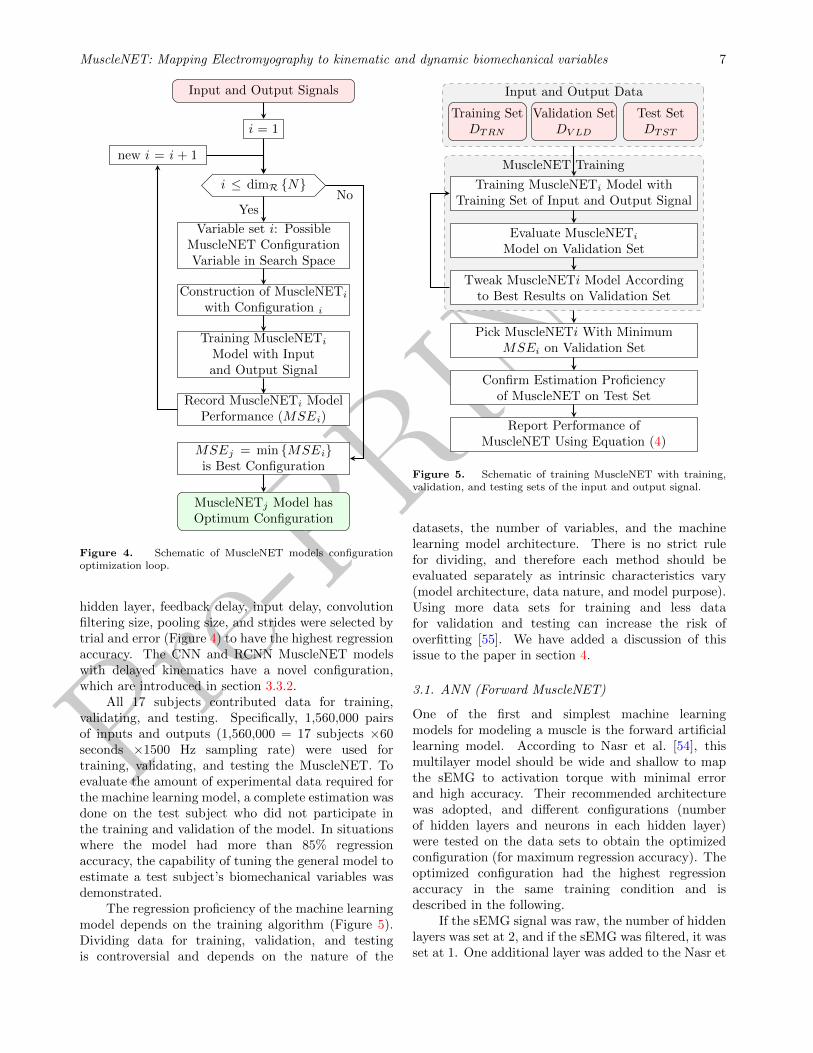
Figure 4. Schematic of MuscleNET models configurationoptimization loop.

hidden layer, feedback delay, input delay, convolutionfiltering size, pooling size, and strides were selected bytrial and error (Figure 4) to have the highest regressionaccuracy. The CNN and RCNN MuscleNET modelswith delayed kinematics have a novel configuration,which are introduced in section 3.3.2.

All 17 subjects contributed data for training,validating, and testing. Specifically, 1,560,000 pairsof inputs and outputs (1,560,000 = 17 subjects ×60seconds ×1500 Hz sampling rate) were used fortraining, validating, and testing the MuscleNET. Toevaluate the amount of experimental data required forthe machine learning model, a complete estimation wasdone on the test subject who did not participate inthe training and validation of the model. In situationswhere the model had more than 85% regressionaccuracy, the capability of tuning the general model toestimate a test subject’s biomechanical variables wasdemonstrated.

The regression proficiency of the machine learningmodel depends on the training algorithm (Figure 5).Dividing data for training, validation, and testingis controversial and depends on the nature of the

MuscleNET Training

Input and Output Data

Training SetDTRN

Validation SetDV LD

Test SetDTST

Training MuscleNETi Model withTraining Set of Input and Output Signal

Evaluate MuscleNETi

Model on Validation Set

Tweak MuscleNETi Model Accordingto Best Results on Validation Set

Pick MuscleNETi With MinimumMSEi on Validation Set

Confirm Estimation Proficiencyof MuscleNET on Test Set

Report Performance ofMuscleNET Using Equation (4)

Figure 5. Schematic of training MuscleNET with training,validation, and testing sets of the input and output signal.

datasets, the number of variables, and the machinelearning model architecture. There is no strict rulefor dividing, and therefore each method should beevaluated separately as intrinsic characteristics vary(model architecture, data nature, and model purpose).Using more data sets for training and less datafor validation and testing can increase the risk ofoverfitting [55]. We have added a discussion of thisissue to the paper in section 4.

3.1. ANN (Forward MuscleNET)

One of the first and simplest machine learningmodels for modeling a muscle is the forward artificiallearning model. According to Nasr et al. [54], thismultilayer model should be wide and shallow to mapthe sEMG to activation torque with minimal errorand high accuracy. Their recommended architecturewas adopted, and different configurations (numberof hidden layers and neurons in each hidden layer)were tested on the data sets to obtain the optimizedconfiguration (for maximum regression accuracy). Theoptimized configuration had the highest regressionaccuracy in the same training condition and isdescribed in the following.

If the sEMG signal was raw, the number of hiddenlayers was set at 2, and if the sEMG was filtered, it wasset at 1. One additional layer was added to the Nasr et

Pre-PRINT


al. [54] model for the described approach as more layersfiltered the raw signal. Since the delayed kinematicsprovided valuable data for the model, the number ofneurons in each layer was set to 4 times the number ofinput signals (for example, for 11 sEMG signals and 3delayed kinematic signals, the number of neurons is 4times 14 or 56). When the inputs were purely sEMGsignals, the number of neurons in each layer was set at5 times the number of input signals (for example, for11 sEMG signals, the number of neurons is 5 times 11or 55). The ANN MuscleNET configuration details aresummarized in Table 1.

The training method was a Levenberg-Marquardtbackpropagation. The maximum epoch was set to2000. The maximum elapsed time was set to 6 hours.

3.2. RNN (Recurrent MuscleNET)

Since the muscle dynamics and joint motion relyon motion history, we hypothesized that RecurrentNeural Networks might have better accuracy in musclemodeling. This model has feedback from the output tothe inputs. After training the nonlinear autoregressivewith external input (NARX) networks, the output timeseries was predicted with the past output values (thefeedback input) and the external input time series(sEMG signal and delayed kinematics). The generalarchitecture was adopted from [13], and differentconfigurations (number of hidden layers, neurons ineach hidden layer, feedback delays, and input delays)were tested using the data sets to obtain the optimizedconfiguration that had the highest regression accuracyfor the same training condition.

The number of hidden layers was 2. The numberof neurons was 3 times the number of input signalswhen the inputs had delayed kinematic signals and 4times the input signals when the inputs did not consistof the delayed kinematics. The feedback delays werethen set to the last 7 signal values. Since different inputdelays did not impact accuracy, we set the input delaysto zero or used the current input value. The details ofthe RNN MuscleNET configuration are summarized inTable 2, and an example of RNN MuscleNET for 11filtered sEMG signals and 3 delayed kinematic signalsis depicted in Figure 6. The maximum epoch trainingmethod and the maximum elapsed time were the sameas for the ANN.

3.3. CNN (Convolutional MuscleNET)

We initially adopted the CNN and RCNN configura-tions from prior work [30, 32, 36] and tested differentconfigurations (number of convolutional layers, convo-lution filtering size, pooling size, strides, neurons infully connected layer, activation function) using thedata sets to obtain the following configuration, which

Sequence Input with 11 × 1 Dimension

Fully Connected Layer with 42 NeuronsActivation Function: Linear

Fully Connected Layer with 42 NeuronsActivation Function: Linear

Fully Connected Layer with 1 NeuronsActivation Function: Tan-sigmoid

Tap-delayed Line1 : 7

Sequence Output with 1 × 1 Dimension

11× 1 output size

1× 42

1× 42

1× 1 output size

7× 1

Hid

den

Lay

ers

Ou

tpu

tL

ayer

Figure 6. Schematic of the RNN MuscleNET for combinedinput of 11 filtered sEMG and three delayed kinematic signals.

had the highest regression accuracy for the same train-ing condition. The configurations of CNN and RCNNMuscleNET with a delayed kinematic signal are novelin terms of parallel structures for delayed kinematicsignal input.

Since there were two different input signals (sEMGsignals and delayed kinematic signals), the CNNmodels’ configurations were categorized into 4 differentshapes based on the input’s conditions. First, wedescribe the CNN generic configuration and then thedifferent configurations in the following paragraph.

Generally, the typical configuration consists of aninput group, the convolution groups, and an outputgroup. First, the input group is a sequence inputlayer that gets an image from the input signals.Secondly, the first layer of convolution groups is afolding sequence layer, and the last one is an unfoldingsequence layer. Finally, the output group consists of 4layers: the flatten layer, a fully connected layer with anoutput size of 50 neurons, a fully connected layer withan output size of 1 neuron, and finally, the regressionlayer.

Precisely, the number of signals made the image’sheight (for example, for 11 sEMG signals and 3 delayedkinematic signals, the image’s height was 14). Theimage’s width is relevant to the history of sEMG signalsthat we want to filter by CNN or RCNN. Since themaximum human motion frequency is roughly 6 Hz[56], we recommend using a maximum of 7 Hz. We didnot propose to use less than 5 Hz since the number ofdata points increases for the CNN or RCNN, slowingmodel processing. For data with a 1500 Hz sample rate,we used 250 points for the image’s width, which is 6Hz of the data. In summary, the input image size was

Pre-PRINT


Table 1. Detail of ANN MuscleNET Model Configuration.

#Inputs Configuration Outputs

Nu

mb

erof

Neu

ron

s

Filte

red

sEM

GR

aw

sEM

GD

elayed

Kin

emati

c

Siz

e Number of Activation Function in

Siz

e

Hid

den

Layer

s

Neu

ron

sin

Each

Hid

den

Layer

Hid

den

Layer

Ou

tpu

tL

ayer

1 X 11×1 1 55 Tan-sigmoid Tan-sigmoid 1×1 7162 X 11×1 2 55 Tan-sigmoid Tan-sigmoid 1×1 37963 X X 14×1 1 56 Tan-sigmoid Tan-sigmoid 1×1 8974 XX 14×1 2 56 Tan-sigmoid Tan-sigmoid 1×1 4089

Table 2. Detail of RNN MuscleNET Model Configuration.

#Inputs Configuration Outputs

Nu

mb

erof

Neu

ron

s

Filte

red

sEM

GR

aw

sEM

GD

elayed

Kin

emati

c

Siz

e Number of Activation Function in

Siz

e

Hid

den

Layer

sN

euro

ns

inE

ach

Hid

den

Layer

Inp

ut

Del

ays

Fee

db

ack

Del

ay

Hid

den

Layer

Ou

tpu

tL

ayer

5 X 11×1 2 44 1 7 Tan-sigmoid Tan-sigmoid 1×1 20246 X 11×1 2 44 1 7 Tan-sigmoid Tan-sigmoid 1×1 20247 X X 14×1 2 42 1 7 Tan-sigmoid Tan-sigmoid 1×1 18488 XX 14×1 2 42 1 7 Tan-sigmoid Tan-sigmoid 1×1 1848

S1(t−249) S1(t−248) S1(t−247) · · · S1(t)S2(t−249) S2(t−248) S2(t−247) · · · S2(t)S3(t−249) S3(t−248) S3(t−247) · · · S3(t)

......

.... . .

...S11(t−249)S11(t−248)S11(t−247) · · · S11(t)θ(t′−249) θ(t′−248) θ(t′−247) · · · θ(t′)

θ(t′′−249) θ(t′′−248) θ(t′′−247) · · · θ(t′′)

θ(t′′′−249) θ(t′′′−248) θ(t′′′−247) · · · θ(t′′′)

250

14

sEM

GK

inem

atic

Figure 7. A sample of the input image made from sEMGsignals and delayed kinematic signals used as the input ofthe CNN or RCNN configuration of MuscleNET. The delayedshoulder elevation joint angle, velocity, and acceleration are θ(t′),θ(t′′), and θ(t′′′), respectively (t′, t′′, and t′′′ are the delayedtimes).

11 by 250 for the sEMG signals input and was 14 by250 for inputs consisting of sEMG signals plus delayedkinematics (Figure 7). The current data is located onthe image’s right, and the 249 previous data is locatedat the left of the image. The sequential input layerhandled importing this 1D image. It is noteworthy thatsignals should not have the same rate as the samplingrate when making the images from the signals. Sincethe model’s delay might be around 0.05 sec or 20 Hz, weused a slower rate of making images. We used 0.1 sec

for making the images, and at each time, must use thecurrent signals and 249 of the previous signals to makethe image, then wait for 0.1 sec to make the followingimage. This way, we considered the model’s delay andsystem to use the model for model-based control ofbiomechatronic devices. Using an image composed ofsEMG signals and delayed kinematic signals is a novelapproach.

The training method was Adam (adaptive mo-ment estimation) optimizer with a unit threshold forthe gradient. The learning rate used for training wasset to 0.001. The maximum epoch was set to 500. Themini-batch size (a subset of the training set) for eachtraining iteration was set to 2000.

The convolution groups were unique for thedifferent input signals (with or without delayedkinematics and raw or filtered sEMG signals). In thefollowing sections, the CNN models are explained indetail for each input signal combination.

3.3.1. Without Delayed Kinematic Signals Whenonly the raw sEMG signals were the input image’sconstructor, there were 8 layers in the convolutionalgroups, and they were taken serially (Figure 8). Allgroups had a 2-D convolutional layer that was appliedto slide convolutional filters with a filter size of height1 and width 3. The output of this layer had thesame size as the input when the stride equaled 1.The step size for traversing the input was 1 verticallyand was 1 horizontally. Groups 1, 2, 7, and 8 had

Pre-PRINT


Sequence Input with11× 250× 1 Dimension

Folding Sequence

1× 3 2-D Convolution, 16

G1

1× 3 Average 2-D Pooling, stride [1, 3]


G2



G3



G4



G5


G7


G6


G8


Unfolding SequenceFlatten Layer

Fully Connected Layer with 50 NeuronsFully Connected Layer with 1 Neuron

Regression Output

11× 250× 1 output size

11× 83× 16

11× 30× 16

11× 10× 64

11× 3× 64

11× 1× 64

11× 1× 64

11× 1× 16


Inp

ut

Gro

up

Con

volu

tion

Gro

up

sO

utp

ut

Gro

up

Figure 8. Schematic of the convolutional MuscleNET forraw sEMG signal input only, including convolutional layers,average pooling layers, and fully connected layer. The batchnormalization and the rectified linear unit after the convolutionallayers in each group have not been shown for simplicity. Theconvolutional layers and the average pooling layers have the samepadding.

16 neurons, and groups 3 to 6 had 64 neurons inthe convolutional layer (the number of channels orfeature maps). All 8 groups had a batch normalizationlayer that normalized each input channel across amini-batch size. We used this batch normalizationlayer to accelerate the networks’ learning and reducethe network initialization sensitivity. Moreover, all8 groups had a Rectified Linear Unit (ReLU) layerthat implemented a threshold operation to each input

element, where any negative value was set to zero.Only the first 5 groups had average pooling layers fordown-sampling by dividing the input into rectangularpooling areas and calculating each area’s averagevalues. The pooling region’s dimensions had a heightof 1 and a width of 3. The vertical step size was 1, andthe horizontal step size was 3. The vertical unit sizefor the pooling layer’s stride was utilized because thesEMG signals should be filtered separately.

All in all, the first 5 groups had a 2-D convolutionlayer, a batch normalization layer, a ReLU layer, anda 2-D average pooling layer. The 6 to 8 groups hada 2-D convolution layer, a batch normalization layer,and a ReLU layer.

For input images constructed with the filteredsEMG signals, group 7 was removed, and group6 was connected to group 8. The convolutionalneural network configuration for raw sEMG signal andwithout the delayed kinematics signal was quite similarto the model proposed by Ameri et al. [34], whichallowed for a direct comparison with our new model.

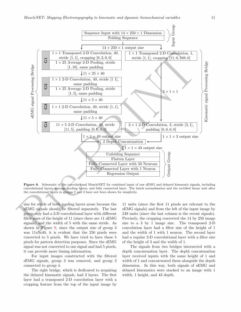
3.3.2. With Delayed Kinematic Signals Since theorigin of the delayed kinematic and sEMG signals aredifferent, they first should be filtered with differentconvolutional layers separately. To this end, weinnovated a parallel structure with two separatebridges. The first bridge handles filtering the sEMGsignals, and the second one relates to delayed kinematicusage. Finally, both bridges intersect, and all data wasused for modeling the mapping of the input (sEMGand delayed kinematic signals) to the output signals.This novel configuration for separating different signalsfrom the image is shown in Figure 9.

The left bridge, dedicated to filtering the sEMGsignals, had 4 groups for raw sEMG signals. The firstgroup had a transposed 2-D convolution layer withan additional feature of cropping the image. Thisnew feature shaved the input image (that is, thecombination of sEMG and delayed kinematic signals).The transposed 2-D convolution layer’s output size wasreduced by cropping from the bottom of the input by 3units since the last 3 pixels are relevant to the delayedkinematic signals. The transposed 2-D convolutionlayer and 2-D convolutional layers at groups 2 and 3had a filter size of the height of 1 and the width of1. All convolutional layers had 40 neurons each. Thestep size for traversing the input was 1 vertically andwas 1 horizontally for all convolutional layers. Thefirst two groups had a ReLU layer and average poolinglayers for down-sampling. Both pooling layers had apooling region’s dimensions with a height of 1 and awidth of 25. However, the first one’s stride at the firstlayer was 10, and the second one at the second layerwas 5 in the horizontal direction. The vertical unit

Pre-PRINT


Sequence Input with 14× 250× 1 DimensionFolding Sequence

1× 1 Transposed 2-D Convolution, 40,stride [1, 1], cropping [0, 3, 0, 0]

G1

1× 25 Average 2-D Pooling, stride[1, 10], same padding

1× 1 2-D Convolution, 40, stride [1 1],same padding

G2


G3

1× 1 2-D Convolution, 40, stride [1, 1],same padding

G4

11× 5 2-D Convolution, 40, stride[11, 5], padding [0, 0, 0, 0]

2 Depth Concatenation


3× 1 2-D Convolution, 3, stride [3, 1],padding [0, 0, 0, 0]


Fully Connected Layer with 50 NeuronsFully Connected Layer with 1 Neuron

Regression Output


11× 25× 40

11× 5× 40

11× 5× 40

3× 1× 1

1× 1× 40 output size 1× 1× 3 output size


Inp

ut

Gro

up

sEM

Gsi

gn

al

Pro

cess

ing

Bri

dge

Kin

emati

csi

gn

al

Pro

cess

ing

Bri

dge

Ou

tpu

tG

rou

p

Figure 9. Schematic of the convolutional MuscleNET for combined input of raw sEMG and delayed kinematic signals, includingconvolutional layers, average pooling layers, and fully connected layer. The batch normalization and the rectified linear unit afterthe convolutional layers in groups 2 and 3 have not been shown for simplicity.

size for stride of both pooling layers arose because thesEMG signals should be filtered separately. The lastgroup only had a 2-D convolutional layer with differentfilter sizes of the height of 11 (since there are 11 sEMGsignals) and the width of 5 with the same stride. Asshown in Figure 9, since the output size of group 3was 11x5x40, it is evident that the 250 pixels wereconverted to 5 pixels. We have tried to have these 5pixels for pattern detection purposes. Since the sEMGsignal was not converted to one signal and had 5 pixels,it can provide more timing information.

For input images constructed with the filteredsEMG signals, group 3 was removed, and group 2connected to group 4.

The right bridge, which is dedicated to acquiringthe delayed kinematic signals, had 2 layers. The firstlayer had a transposed 2-D convolution layer with acropping feature from the top of the input image by

11 units (since the first 11 pixels are relevant to thesEMG signals) and from the left of the input image by249 units (since the last column is the recent signals).Precisely, the cropping converted the 14 by 250 imagesize to a 3 by 1 image size. The transposed 2-Dconvolution layer had a filter size of the height of 1and the width of 1 with 1 neuron. The second layerhad a regular 2-D convolutional layer with a filter sizeof the height of 3 and the width of 1.

The signals from two bridges intersected with adepth concatenation layer. The depth concatenationlayer received inputs with the same height of 1 andwidth of 1 and concatenated them alongside the depthdimension. In this way, both signals of sEMG anddelayed kinematics were stacked to an image with 1width, 1 height, and 43 depth.

Pre-PRINT


Sequence Input with 14× 250× 1 DimensionFolding Sequence


G1


1× 1 2-D Convolution, 40, stride [1 1],same padding

G2


G3

1× 1 2-D Convolution, 40, stride [1, 1],same padding

G4

11× 5 2-D Convolution, 40, stride[11, 5], padding [0, 0, 0, 0]

2 Depth Concatenation


3× 1 2-D Convolution, 3, stride [3, 1],padding [0, 0, 0, 0]


LSTM Layer with 50 NeuronsActivation Function of Neurons: Hyperbolic Tangent function

Activation Function of the Gate: Sigmoid FunctionOutput: last time step of the sequenceFully Connected Layer with 1 Neuron

Regression Output


11× 25× 40

11× 5× 40

11× 5× 40

3× 1× 1

1× 1× 40 output size 1× 1× 3 output size


Inp

ut

Gro

up

sEM

Gsi

gn

al

Pro

cess

ing

Bri

dge

Kin

emati

csi

gn

al

Pro

cess

ing

Bri

dge

Ou

tpu

tG

rou

p

Figure 10. Schematic of the RCNN MuscleNET for combined input of raw sEMG and delayed kinematic signals, includingconvolutional layers, average pooling layers, and a Long Short-Term Memory (LSTM) layer. The batch normalization and therectified linear unit after the convolutional layers in groups 2 and 3 have not been shown for simplicity.

3.4. RCNN (Recurrent Convolutional MuscleNET)

The RCNN’s configuration approximates the CNN; theonly difference is in the output group’s layers. The fullyconnected layer with an output size of 50 neurons inthe CNN was changed to a Long Short-Term Memory(LSTM) layer with 50 hidden units. Additionally,the output of the LSTM was the last time step ofthe sequence in the RCNN. The activation functionto update the cell and hidden state was set to bethe hyperbolic tangent function, and the activationfunction to apply to the gates was the sigmoid.

The schematic of the RCNN MuscleNET for thecombined input of raw sEMG and delayed kinematicsignals is shown in Figure 10. The input image,

the input group, and the general output group wereintroduced in section 3.3. The details of the sEMGsignal processing and kinematic signal processing havebeen presented in section 3.3.2.

4. Results and Discussion

This section presents the data ratio analysis for thetraining, validation, and testing of subject-specific andgeneral models. Second, the volume of experimentaldata for complete estimation with a general modelwas assessed. Third, eighty different configurationsof MuscleNET with different input conditions (rawor filtered sEMG signal, without or with delayed

Pre-PRINT


Subject-specific Model

General Model

D1 D2 · · · Dn−3 Dn−2 Dn−1 Dn

Train Set Test Set

Validation Set

Overlap

D1 D2 · · · Dn−3 Dn−2 Dn−1 Dn

Train Set Test Set

Validation Set

Overlap

Figure 11. Visual representation of dividing data base intotraining, validation, and testing sets for subject-specific andgeneral models.

kinematic signals) and different outputs (5 differentbiomechanical signals) were compared in terms of theperformance, training time, and maximum inferencetime. Finally, samples of complete estimation forrandom subjects were presented. For training ofthe MuscleNET, a personal computer with an Intel®

CoreTM i7-3370 CPU @ 3.40GHz processor and 16.0GB memory was used.

4.1. Dividing Ratio and Data Volume

To study the division of data for training, validation,and testing concerning maximum estimation accuracywithout overfitting, we trained the models withdifferent ratios of training, validation, and test data.We have assessed the different ratios, and twocombinations produced the best results for the subject-specific and general models (Figure 11). The subject-specific model was tuned for maximum estimationaccuracy of validation data with 94.1% of data fortraining, 5.9% of data for exporting-and-validation(note that validation data overlaps with training data),and 5.9% unique data for testing. The general modelwas achieved with 94.1%, 23.5%, and 5.9% of datafor training, exporting-and-validation, and testing,respectively. The overlap of validation and trainingsets may decrease in the case of reach experimentaldata availability.

For the subject-specific model, 16 subjects (94.1%of total data) were selected for training, and oneof them (5.9% of total) was present in training andvalidation simultaneously. This subject plays the roleof stopping the training process and signaling theexport of the final model with the lowest MSE. The

0.2 0.4 0.6 0.8

Target

0.2

0.4

0.6

0.8

Outp

ut ~

= 1

*Targ

et +

0.0

02

Training: R=0.9982

Data

Fit

Y = T

0.2 0.4 0.6 0.8

Target

0.2

0.4

0.6

0.8

Outp

ut ~

= 1

*Targ

et +

-0.0

087

Validation: R=0.99731

Data

Fit

Y = T

0.2 0.4 0.6 0.8

Target

0.2

0.4

0.6

0.8

Outp

ut ~

= 0

.9*T

arg

et +

-0.0

036 Test: R=0.97761

Data

Fit

Y = T

0.2 0.4 0.6 0.8

Target

0.2

0.4

0.6

0.8

Outp

ut ~

= 0

.99*T

arg

et +

0.0

029 All: R=0.99508

Data

Fit

Y = T

Figure 12. The machine learning training, validation, andtesting regression of a subject-specific model of RNN MuscleNETwith filtered sEMG and delayed kinematic signals input and jointangle output. The test subject did not participate in trainingand validation.

other subject who did not participate in training andvalidation was selected as the test set. We observedthat the regression accuracy for the validation subjectreached 99.7% (Figure 12). However, the test resultwas not as successful (97.7%). In other words, sincethe training stopped and was exported based on theregression of one subject validation, the model issubject-specific for the validation subject and a lessgeneral model for testing data sets. The machinelearning model has less regression accuracy for testingwith different data sets (any subjects other than thoseused for validation). Although this trained MuscleNETwith one validation subject’s data has high regressionaccuracy for the validation subject, the model issubject-specific and should not be used for generalpurposes. If the EMG signals were not stochasticand time-varying, the regression would be greaterthan the amount reached already. In addition, froma biomechanical perspective, the maximum muscleforce, muscle attachment configuration, and musclepassive and active functions (biomechanical musclefeatures) are different between different subjects.Thus, selecting a small amount of data for validation(for example, only one subject) decreases the breadthof biomechanical muscle features for different subjectsand increases the validation accuracy for the subject-specific model.

For the general model, we found that 23.5% ofdata (4 subjects) for validation gave better resultsthan 5.9% of data (1 subject) used for subject-specific

Pre-PRINT


0.2 0.4 0.6 0.8

Target

0.2

0.4

0.6

0.8

Outp

ut ~

= 0

.99*T

arg

et +

0.0

037 Training: R=0.99688

Data

Fit

Y = T

0.2 0.4 0.6 0.8

Target

0.2

0.4

0.6

0.8

Outp

ut ~

= 1

*Targ

et +

-0.0

014

Validation: R=0.99706

Data

Fit

Y = T

0.2 0.4 0.6 0.8

Target

0.2

0.4

0.6

0.8

Outp

ut ~

= 1

*Targ

et +

0.0

14

Test: R=0.99209

Data

Fit

Y = T

0.2 0.4 0.6 0.8

Target

0.2

0.4

0.6

0.8

Outp

ut ~

= 1

*Targ

et +

0.0

039

All: R=0.99588

Data

Fit

Y = T

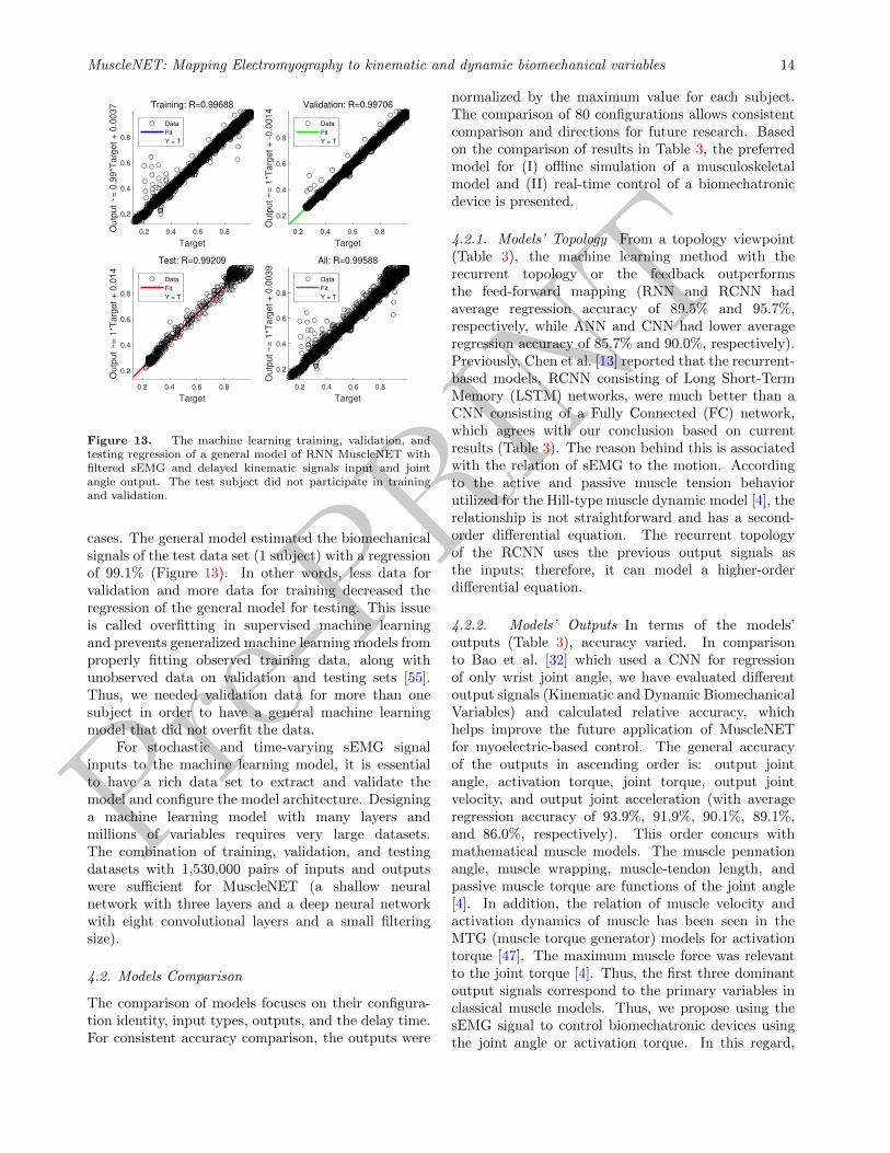
Figure 13. The machine learning training, validation, andtesting regression of a general model of RNN MuscleNET withfiltered sEMG and delayed kinematic signals input and jointangle output. The test subject did not participate in trainingand validation.

cases. The general model estimated the biomechanicalsignals of the test data set (1 subject) with a regressionof 99.1% (Figure 13). In other words, less data forvalidation and more data for training decreased theregression of the general model for testing. This issueis called overfitting in supervised machine learningand prevents generalized machine learning models fromproperly fitting observed training data, along withunobserved data on validation and testing sets [55].Thus, we needed validation data for more than onesubject in order to have a general machine learningmodel that did not overfit the data.

For stochastic and time-varying sEMG signalinputs to the machine learning model, it is essentialto have a rich data set to extract and validate themodel and configure the model architecture. Designinga machine learning model with many layers andmillions of variables requires very large datasets.The combination of training, validation, and testingdatasets with 1,530,000 pairs of inputs and outputswere sufficient for MuscleNET (a shallow neuralnetwork with three layers and a deep neural networkwith eight convolutional layers and a small filteringsize).

4.2. Models Comparison

The comparison of models focuses on their configura-tion identity, input types, outputs, and the delay time.For consistent accuracy comparison, the outputs were

normalized by the maximum value for each subject.The comparison of 80 configurations allows consistentcomparison and directions for future research. Basedon the comparison of results in Table 3, the preferredmodel for (I) offline simulation of a musculoskeletalmodel and (II) real-time control of a biomechatronicdevice is presented.

4.2.1. Models’ Topology From a topology viewpoint(Table 3), the machine learning method with therecurrent topology or the feedback outperformsthe feed-forward mapping (RNN and RCNN hadaverage regression accuracy of 89.5% and 95.7%,respectively, while ANN and CNN had lower averageregression accuracy of 85.7% and 90.0%, respectively).Previously, Chen et al. [13] reported that the recurrent-based models, RCNN consisting of Long Short-TermMemory (LSTM) networks, were much better than aCNN consisting of a Fully Connected (FC) network,which agrees with our conclusion based on currentresults (Table 3). The reason behind this is associatedwith the relation of sEMG to the motion. Accordingto the active and passive muscle tension behaviorutilized for the Hill-type muscle dynamic model [4], therelationship is not straightforward and has a second-order differential equation. The recurrent topologyof the RCNN uses the previous output signals asthe inputs; therefore, it can model a higher-orderdifferential equation.

4.2.2. Models’ Outputs In terms of the models’outputs (Table 3), accuracy varied. In comparisonto Bao et al. [32] which used a CNN for regressionof only wrist joint angle, we have evaluated differentoutput signals (Kinematic and Dynamic BiomechanicalVariables) and calculated relative accuracy, whichhelps improve the future application of MuscleNETfor myoelectric-based control. The general accuracyof the outputs in ascending order is: output jointangle, activation torque, joint torque, output jointvelocity, and output joint acceleration (with averageregression accuracy of 93.9%, 91.9%, 90.1%, 89.1%,and 86.0%, respectively). This order concurs withmathematical muscle models. The muscle pennationangle, muscle wrapping, muscle-tendon length, andpassive muscle torque are functions of the joint angle[4]. In addition, the relation of muscle velocity andactivation dynamics of muscle has been seen in theMTG (muscle torque generator) models for activationtorque [47]. The maximum muscle force was relevantto the joint torque [4]. Thus, the first three dominantoutput signals correspond to the primary variables inclassical muscle models. Thus, we propose using thesEMG signal to control biomechatronic devices usingthe joint angle or activation torque. In this regard,

Pre-PRINT


Table 3. Comparison of regression accuracy for 80 models: 16 MuscleNET configuration times 5 output signals.Model Properties Regression (%)

#

Con

figu

rati

on

Iden

tity Inputs

Nu

mb

erof

Neu

ron

sor

Vari

ab

les

Maxim

um

Infe

ren

ceT

ime

(mic

rose

con

d) Normalized Output

Signal with a 1×1 Size

Aver

age

Filte

red

sEM

GR

aw

sEM

GD

elayed

Kin

emati

c

Siz

e Kinematics Dynamics

Join

tA

ngle

Join

tV

eloci

ty

Join

tA

ccel

erati

on

Join

tT

orq

ue

Act

ivati

on

Torq

ue

1

AN

N

X 11×1 716 6 91.1 81.7 79.2 87.4 89.9 85.9

85.72 X 11×1 3796 10 81.1 69.2 65.9 80.5 85.0 76.33 X X 14×1 897 6 96.9 93.7 87.2 92.2 93.9 92.84 XX 14×1 4089 10 95.1 88.9 78.7 86.2 90.0 87.85

RN

N

X 11×1 2024 12 94.9 87.7 81.3 90.4 91.6 89.2

89.56 X 11×1 2024 12 86.7 71.4 69.3 81.4 85.4 78.87 X X 14×1 1848 12 98.5 98.2 95.0 94.6 95.6 96.48 XX 14×1 1848 12 97.6 97.1 92.9 88.6 91.2 93.59

CN

N

X 11×250 62437 1400 92.2 85.5 85.5 88.5 90.2 88.4

90.010 X 11×250 62485 1500 93.8 89.6 86.6 91.4 91.8 90.611 X X 14×250 10035 1200 92.7 87.7 86.6 89.4 90.7 89.412 XX 14×250 13825 1300 94.6 90.1 88.4 91.6 92.6 91.513

RC

NN

X 11×250 125387 1900 96.3 96.1 94.9 94.7 95.7 95.5

95.714 X 11×250 125435 2000 96.4 96.2 94.9 94.9 95.9 95.715 X X 14×250 108785 1300 96.5 96.2 94.9 94.8 95.8 95.616 XX 14×250 110425 1350 97.2 96.6 95.0 94.9 95.8 95.9

Average 93.9 89.1 86.0 90.1 91.9

since most robotic servo motors have a PID positioncontrol, using the sEMG as the input of the controlalgorithm and the joint angle as a command to the low-level actuator control is more straightforward. Anothermethod is using a force/torque-based control algorithmfor biomechatronic devices. With the sEMG used asthe input, the machine learning model can estimatethe activation torque using an MTG model [49]. Thejoint torque can be calculated and commanded to thelow-level control loop or the robot actuator. Theactivation torque’s superiority over joint torque arisesfrom consideration of the passive and active torqueimpact of muscle in the MTG model [47,49].

4.2.3. Models’ Inputs From the kinematic inputstandpoint, using the delayed kinematic signals alongwith the sEMG signals positively affected the model’saccuracy (using delayed kinematic signals resulted inan average regression accuracy of 92.9% while not usingthose signals resulted in a lower average regressionaccuracy of 87.6%). It is noteworthy to mentionthat the Hill-type muscle model’s inputs [4] are thejoint angle, velocity, and acceleration, along with thesEMG signal. Thus, using the kinematic signals alongwith the sEMG signal, for the first time, is noveland increased model accuracy. Indeed, incorporatingthe delayed kinematic signals decreased the regressionerror from 50% to 20%. For example, using thedelayed kinematic signals in row 12 in Table 3 providesmore accuracy than row 10, which results from the

0 200 400 600 800 10000

0.2

0.4

0.6

0.8

RM

SE

Final Validation Performance (RMSE) is 0.025774

Training Validation

0 200 400 600 800 1000

Iteration

0

0.05

0.1

0.15

0.2

Lo

ss

Final Validation Loss is 0.00033215

Figure 14. The RCNN training (solid) and validation (dashed)rates for 1000 iterations. However, the training procedure couldbe stopped at 500 iterations.

model proposed by Ameri et al. [34]. Using thedelayed signals instead of the current signals reflectsthe need to consider electrical and computationaldelays. Moreover, for real-time control of an actual bio-robot, the delay must be considered in the modeling.For the simulation of the musculoskeletal model,delayed signals are unnecessary. From the sEMGinput perspective, the result provided two distinctconclusions regarding other input conditions: raw or

Pre-PRINT


0 10 20 30 40 50 600

0.5

1

Norm

aliz

ed J

oin

g A

ngle

Test Subject 12 (Male, Age: 23 years , Height: 1.78 m, Weight: 88.5 Kg)

Target RNN (R: 98.5%) RCNN (R: 97.2%)

0 10 20 30 40 50 60

Time (s)

0

0.5

1

Norm

aliz

ed A

ssis

tive T

orq

ue


Figure 15. The performance of RNN and RCNN MuscleNET on random test data for users’ joint angle (top) and joint torquetrajectory (bottom).

0 10 20 30 40 50 600

0.5

1

Norm

aliz

ed J

oin

g A

ngle

Test Subject 9 (Male, Age: 22 years , Height: 1.8 m, Weight: 69.5 Kg)


0 10 20 30 40 50 60

Time (s)

0

0.5

1

Norm

aliz

ed A

ssis

tive T

orq

ue


Figure 16. The test of RNN and RCNN MuscleNET for second random non-used user data for training users’ joint angle (top)and joint torque trajectory (bottom).

filtered sEMG signal. First, for the ANN and RNNmodels, the models’ accuracy was much better whenthe inputs were filtered signals (filtered sEMG signalsyielded average regression accuracy of 91.1%, while rawsignals yielded average regression accuracy of 84.4%).

Hence, the ANN and RNN models should not be usedfor filtering the raw signals. The results revealed thecapability of the convolutional models in filtering thesignals and confirm the superiority of using raw sEMGsignals as the inputs of the CNN and RCNN models.

Pre-PRINT


Dynamic Model of Human Skeletal Systemp = M (q)

−1[Q + F (p,q )]

Transformation of Position Derivative to Velocityq = h (p,q, t)

RNNMuscleNET

FilteredsEMG

∫Memory

Motionp, q p, q

p

Q

Figure 17. Schematic of a musculoskeletal model simulation (for example, for sport engineering purposes or musculoskeletalanalysis). MuscleNET acts as a muscle model using the filtered sEMG, joint position, velocity, and acceleration. MuscleNET’soutput is the joint torque τh supplied to the dynamic model for forward dynamic simulation.

4.2.4. Models’ Delay Since real-time control ofbiomechatronic devices requires a minimal delay, thisfactor should be considered. Comparison of thesystem’s delay is controversial since the signal filteringdelay should be considered as well. Subsequently,filtering the raw sEMG signal has a specific delaydue to low-pass filtering. The delay in filtering theraw signals should be considered with the modeldelay to compute the total delay. In this regard,the models’ delay with the filtered sEMG signalsexceeds expectations. All the control methods had anoperation delay of less than 2 milliseconds (Table 3)because of shallow configuration (not having too manylayers), which is quick for real-time control purposes.Compared to sEMG frequency-based input [35,36], theMuscleNET is much faster and works in real-time sinceprior research [35, 36] initially converted sEMG signalto sEMG frequency bands, which is an offline andtime-consuming conversion. Moreover, sEMG-basedclassification of hand or wrist gestures [5,6,12,17,30,31]requires additional sEMG history compared to RNNMuscleNET which mainly uses the signal value and afaster regression. The Ameri et al. [34] model also hasfive times more variables than CNN MuscleNET withdelayed kinematic input, indicating that MuscleNETincurs less computation cost and has less delay thanthat model [34].

4.3. Testing and Demonstration

These findings motivated re-learning of two specificmodels and comparison of their results. In thosemodels, the outputs were the joint angle and activationtorque. The two models were (I) RNN with filteredsEMG signals plus delayed kinematics and (II) RCNNwith raw sEMG signals plus delayed kinematics. Forre-training of the RNN, the maximum elapsed timewas set to 12 hours. For re-training of the RCNNMuscleNET, the maximum epoch was set to 1000.The rest of the training options were the same as theprevious training step. As an example, the RCNNtraining and validation error rates for 1000 iterationsare presented (Figure 14). The performance of RNNand RCNN MuscleNET for (a) joint angle and (b)

activation torque trajectory with a user dataset thathad not been used for training is shown in Figure15. The RCNN MuscleNET followed the target values,which were the normalized joint angle and joint torque.Another random subject data was used to evaluatethe model (Figure 16). This complete estimation ofthe biomechanical signals of random subjects, who didnot participate in training and validation of the model,had 96.9% accuracy. The result showed that the novelmodel configuration, using delayed kinematic signals,the optimum model configuration, the given amount ofdata, and the optimum division for training, validation,and testing successfully achieved the goal. The amountof experimental data (1530000 pairs of inputs andoutputs) was sufficient to reach this regression accuracyfor estimation tests.

4.4. Application

Two specific applications for (i) RNN MuscleNET and(ii) RCNN MuscleNET emerge from these findings:

(i) Using RNN MuscleNET with inputs of filteredsEMG and delayed kinematic signals could replacemuscles in musculoskeletal models.The output of the MuscleNET can be jointelevation torque or activation torque, and theoutput of the MuscleNET should be used as theinput of the skeletal dynamic model. MuscleNETand the skeletal model’s total system can beused in the forward dynamic simulation of amusculoskeletal model (for example, for clinical orsport engineering purposes) (Figure 17).

(ii) For biomechatronic purposes, the RCNN Muscle-NET, with raw sEMG and delayed kinematic sig-nals, can be used as an interpreter of the sEMGsignals.The output of RCNN MuscleNET is commandedto the low-level control loop of biomechatronic sys-tems (Figure 18). Applications of the method mayinclude controlling assistive/resistive robots, ex-oskeletons, or prostheses [1, 57].

Pre-PRINT


Biomechatronic System

Sensors &Actuators

Model-based Controller

MechatronicDevice

MusculoskeletalSystem

ReactionWrench

KinematicConstraint

Human MotorControl

External Load

Actuator

Passive

TorqueSensor

PositionSensor

sEMGSensor

Low-levelBuilt-inServo

Controller

Mid-levelController:Assistive or

Resistive Law

RCNNMuscleNET

∆∆t

∆∆t

τe

θe

v

τf

θf

τact

θt+1

Raw sEMG Signal

θfθf

Figure 18. Schematic for controlling an exoskeleton, a prosthesis, or a rehabilitation robot using MuscleNET as a muscle modelfor converting the raw sEMG, joint feedback position θf , velocity θf , and acceleration θf to activation torque τact. The low-levelcontroller is responsible for controlling the mechatronic system by desired torque τe or angle θe according to the output of mid-levelcontroller.

5. Conclusion

An alternative solution to mathematical muscle mod-eling using regression RNN and CNN-based sEMG sig-nals is proposed. The model’s performance and qual-ity metrics were compared across 80 different machinelearning regression-based schemes with various condi-tions. The conditions consisted of (I) different kindsof outputs: 3 kinematic signals (joint angle, velocity,and acceleration) and 2 dynamic signals (joint torqueand activation torque), (II) different input conditions:using delayed kinematic signals, raw, or filtered sEMGsignals, and (III) different kinds of neural network con-figurations: ANN, RNN, CNN, and RCNN. The twomodels of (A) RNN with delayed kinematic signal andfiltered sEMG signals inputs and (B) RCNN with de-layed kinematic and raw sEMG signal inputs outper-formed the other schemes in terms of estimation accu-racies. The high performance of the recurrent-basedmodels demonstrated their ability to learn necessarymotor information from sEMG signals. Further, thesignal filtering capability of the CNN-based models wasestablished. MuscleNET was more accurate in estimat-ing joint angles and activation torque signals than jointvelocity, joint acceleration, and joint torque.

Future work should study the robustness ofMuscleNET to factors such as electrode shift andelectrodes that disconnect during a motion. Moreover,the practical application of MuscleNET to controlan active exoskeleton or prostheses is currently being

pursued by the authors, and should lead to refinementsin the method.

Acknowledgments

The authors acknowledge funding of this research bythe Canada Research Chairs program.

Refrences

[1] Ali Nasr, Brock Laschowski, and John McPhee. Myoelec-tric Control of Robotic Leg Prostheses and Exoskeletons:A Review. In Proceedings of the ASME 2021 Inter-national Design Engineering Technical Conferences andComputers and Information in Engineering Conferenceand Computers and Information in Engineering Confer-ence, Online, Virtual, 2021. ASME.

[2] Mohammadreza Asghari Oskoei and Huosheng Hu. My-oelectric control systems—A survey. Biomedical SignalProcessing and Control, 2(4):275–294, 2007.

[3] Dario Farina, Ning Jiang, Hubertus Rehbaum, AlesHolobar, Bernhard Graimann, Hans Dietl, and Oskar C.Aszmann. The extraction of neural information from thesurface EMG for the control of upper-limb prostheses:Emerging avenues and challenges. IEEE Transactionson Neural Systems and Rehabilitation Engineering,22(4):797–809, 2014.

[4] Jack M. Winters. Hill-Based Muscle Models: A SystemsEngineering Perspective. In Multiple Muscle Systems,pages 69–93. Springer, New York, NY, 1990.

[5] Manfredo Atzori, Matteo Cognolato, and Henning Muller.Deep learning with convolutional neural networksapplied to electromyography data: A resource forthe classification of movements for prosthetic hands.Frontiers in Neurorobotics, 10(SEP):9, 2016.

Pre-PRINT


[6] Ulysse Cote-Allard, Cheikh Latyr Fall, Alexandre Drouin,Alexandre Campeau-Lecours, Clement Gosselin, KyrreGlette, Francois Laviolette, and Benoit Gosselin.Deep Learning for Electromyographic Hand GestureSignal Classification Using Transfer Learning. IEEETransactions on Neural Systems and RehabilitationEngineering, 27(4):760–771, 2019.

[7] Lilah Inzelberg, Moshe David-Pur, Eyal Gur, andYael Hanein. Multi-channel electromyography-basedmapping of spontaneous smiles. Journal of NeuralEngineering, 17(2), 2020.

[8] Feiyun Xiao, Yanyan Chen, and Yanhe Zhu. GADF/GASF-HOG:feature extraction methods for hand movementclassification from surface electromyography. Journal ofNeural Engineering, 17(4), 2020.

[9] Aaron J. Young, Lauren H. Smith, Elliott J. Rouse, andLevi J. Hargrove. Classification of simultaneous move-ments using surface EMG pattern recognition. IEEETransactions on Biomedical Engineering, 60(5):1250–1258, 2013.

[10] Xiaolong Zhai, Beth Jelfs, Rosa H.M. Chan, and ChungTin. Self-recalibrating surface EMG pattern recognitionfor neuroprosthesis control based on convolutional neuralnetwork. Frontiers in Neuroscience, 11(JUL):379, 2017.

[11] Luo Zhizeng, Wang Fei, and Ma Wenjie. Patternclassification of surface electromyography based on ARmodel and high-order neural network. In Proceedingsof the 2nd IEEE/ASME International Conference onMechatronic and Embedded Systems and Applications(MESA), pages 1–6, Beijing, China, 2007. IEEE.

[12] Muhammad Ziaur ur Rehman, Asim Waris, Syed OmerGilani, Mads Jochumsen, Imran Khan Niazi, MohsinJamil, Dario Farina, and Ernest Nlandu Kamavuako.Multiday EMG-Based classification of hand motionswith deep learning techniques. Sensors (Switzerland),18(8):2497, 2018.

[13] Yuyang Chen, Chenyun Dai, and Wei Chen. Cross-Comparison of EMG-to-Force Methods for Multi-DoFFinger Force Prediction Using One-DoF Training. IEEEAccess, 8:13958–13968, 2020.

[14] Ruochen Hu, Xiang Chen, Chengjun Huang, ShuaiCao, Xu Zhang, and Xun Chen. Elbow-flexion forceestimation during arm posture dynamically changingbetween pronation and supination. Journal of NeuralEngineering, 16(6), 2019.

[15] Ning Jiang, Johnny Lg Vest-Nielsen, Silvia Muceli, andDario Farina. EMG-based simultaneous and propor-tional estimation of wrist/hand kinematics in uni-lateraltrans-radial amputees. Journal of NeuroEngineeringand Rehabilitation, 9(1):42, 2012.

[16] Claudio Castellini and Patrick Van Der Smagt. SurfaceEMG in advanced hand prosthetics. Biological Cyber-netics, 100(1):35–47, 2009.

[17] Yu Du, Yongkang Wong, Wenguang Jin, Wentao Wei,Yu Hu, Mohan Kankanhalli, and Weidong Geng. Semi-supervised learning for surface EMG-based gesturerecognition. In IJCAI International Joint Conferenceon Artificial Intelligence, volume 0, pages 1624–1630,Melbourne, Australia, 2017. AAAI Press.

[18] Zhiyuan Lu, Argyrios Stampas, Gerard E. Francisco, andPing Zhou. Offline and online myoelectric patternrecognition analysis and real-time control of a robotichand after spinal cord injury. Journal of NeuralEngineering, 16(3), 2019.

[19] Yoshua Bengio, Aaron Courville, and Pascal Vincent.Representation learning: A review and new perspectives.IEEE Transactions on Pattern Analysis and MachineIntelligence, 35(8):1798–1828, 2013.

[20] Levi J. Hargrove, Blair A. Lock, and Ann M. Simon.Pattern recognition control outperforms conventional

myoelectric control in upper limb patients with targetedmuscle reinnervation. In 35th Annual InternationalConference of the IEEE Engineering in Medicine andBiology Society (EMBC), pages 1599–1602, Osaka,Japan, 2013. IEEE.

[21] Silvia Muceli and Dario Farina. Simultaneous andproportional estimation of hand kinematics from EMGduring mirrored movements at multiple degrees-of-freedom. IEEE Transactions on Neural Systems andRehabilitation Engineering, 20(3):371–378, 2012.

[22] Angkoon Phinyomark, Pornchai Phukpattaranont, andChusak Limsakul. Feature reduction and selectionfor EMG signal classification. Expert Systems withApplications, 39(8):7420–7431, 2012.

[23] Erik Scheme and Kevin Englehart. Training strategiesfor mitigating the effect of proportional control onclassification in pattern recognition-based myoelectriccontrol. Journal of Prosthetics and Orthotics, 25(2):76–83, 2013.

[24] Ann M. Simon, Levi J. Hargrove, Blair A. Lock, andTodd A. Kuiken. Target achievement control test: Eval-uating real-time myoelectric pattern-recognition controlof multifunctional upper-limb prostheses. Journal of Re-habilitation Research and Development, 48(6):619–628,2011.

[25] Angkoon Phinyomark and Erik Scheme. EMG patternrecognition in the era of big data and deep learning. BigData and Cognitive Computing, 2(3):1–27, 2018.

[26] Alex Krizhevsky, Ilya Sutskever, and Geoffrey E. Hinton.ImageNet classification with deep convolutional neuralnetworks. Communications of the ACM, 60(6):84–90,2017.

[27] Ossama Abdel-Hamid, Abdel Rahman Mohamed, HuiJiang, Li Deng, Gerald Penn, and Dong Yu. Convo-lutional neural networks for speech recognition. IEEETransactions on Audio, Speech and Language Process-ing, 22(10):1533–1545, 2014.

[28] Qiaoxiu Wang, Hong Wang, Fo Hu, and Chengcheng Hua.Using convolutional neural networks to decode EEG-based functional brain network with different severity ofacrophobia. Journal of Neural Engineering, 2020.

[29] Yann LeCun, Leon Bottou, Yoshua Bengio, and PatrickHaffner. Gradient-based learning applied to documentrecognition. Proceedings of the IEEE, 86(11):2278–2323,1998.

[30] Ali Ameri, Mohammad Ali Akhaee, Erik Scheme, andKevin Englehart. Real-time, simultaneous myoelectriccontrol using a convolutional neural network. PLoSONE, 13(9):e0203835, 2018.

[31] Weidong Geng, Yu Du, Wenguang Jin, Wentao Wei, Yu Hu,and Jiajun Li. Gesture recognition by instantaneoussurface EMG images. Scientific Reports, 6:36571, 2016.

[32] Tianzhe Bao, Ali Zaidi, Shengquan Xie, and ZhiqiangZhang. Surface-EMG based wrist kinematics estima-tion using convolutional neural network. In 16th Inter-national Conference on Wearable and Implantable BodySensor Networks (BSN), pages 1–4, Chicago, IL, USA,2019. IEEE.

[33] Henrique Dantas, David J. Warren, Suzanne M. Wendelken,Tyler S. Davis, Gregory A. Clark, and V. John Mathews.Deep Learning Movement Intent Decoders Trained withDataset Aggregation for Prosthetic Limb Control. IEEETransactions on Biomedical Engineering, 66(11):3192–3203, 2019.

[34] Ali Ameri, Mohammad Ali Akhaee, Erik Scheme, andKevin Englehart. Regression convolutional neuralnetwork for improved simultaneous EMG control.Journal of Neural Engineering, 16(3):36015, 2019.

[35] Weiming Wangshow, Biao Chen, Peng Xia, Jie Hu, andYinghong Peng. Sensor Fusion for Myoelectric Control

Pre-PRINT


Based on Deep Learning With Recurrent ConvolutionalNeural Networks. Artificial Organs, 42(9):E272–E282,2018.

[36] Peng Xia, Jie Hu, and Yinghong Peng. EMG-Based Es-timation of Limb Movement Using Deep Learning WithRecurrent Convolutional Neural Networks. Artificial Or-gans, 42(5):E67–E77, 2018.

[37] Yixin Liu, Daxin Xin, Jin Hua, and Mengzhao Liu.SEMG Motion Intention Recognition Based on WaveletTime-Frequency Spectrum and ConvLSTM. Journal ofPhysics: Conference Series, 1631(1), 2020.

[38] Rachel L. Whittaker, Nicholas J. La Delfa, andClark R. Dickerson. Algorithmically detectable direc-tional changes in upper extremity motion indicate sub-stantial myoelectric shoulder muscle fatigue during arepetitive manual task. Ergonomics, 62(3):431–443,2019.

[39] Rachel L. Whittaker, Woojin Park, and Clark R.Dickerson. Application of a symbolic motion structurerepresentation algorithm to identify upper extremitykinematic changes during a repetitive task. Journal ofBiomechanics, 72:235–240, 2018.

[40] Dale Avers and Marybeth Brown. Daniels and Worthing-ham’s Muscle Testing: Techniques of Manual Examina-tion and Performance Testing. Elsevier Inc., page 416,2018.

[41] David A. Winter. Biomechanics and Motor Control ofHuman Movement: Fourth Edition. John Wiley & Sons,2009.

[42] Ge Wu, Frans C.T. Van Der Helm, H. E.J. Veeger, MohsenMakhsous, Peter Van Roy, Carolyn Anglin, JochemNagels, Andrew R. Karduna, Kevin McQuade, XuguangWang, Frederick W. Werner, and Bryan Buchholz.ISB recommendation on definitions of joint coordinatesystems of various joints for the reporting of humanjoint motion - Part II: Shoulder, elbow, wrist and hand.Journal of Biomechanics, 38(5):981–992, 2005.

[43] Vandana Phadke, Jonathan P. Braman, Robert F. LaPrade,and Paula M. Ludewig. Comparison of glenohumeralmotion using different rotation sequences. Journal ofBiomechanics, 44(4):700–705, 2011.

[44] James J. Burkitt, Victoria Staite, Afrisa Yeung, DigbyElliott, and James L. Lyons. Effector mass andtrajectory optimization in the online regulation ofgoal-directed movement. Experimental Brain Research,233(4):1097–1107, 2015.

[45] Katherine R.S. Holzbaur, Wendy M. Murray, and Scott L.Delp. A model of the upper extremity for simulatingmusculoskeletal surgery and analyzing neuromuscularcontrol. Annals of Biomedical Engineering, 33(6):829–840, 2005.

[46] R. Dumas, L. Cheze, and J. P. Verriest. Adjustments toMcConville et al. and Young et al. body segment inertialparameters. Journal of Biomechanics, 40(3):543–553,2007.

[47] Keaton A. Inkol, Colin Brown, William McNally, ConorJansen, and John McPhee. Muscle torque generatorsin multibody dynamic simulations of optimal sportsperformance. Multibody System Dynamics, 50(4):435–452, 2020.

[48] Ali Nasr and John McPhee. Control-Oriented MuscleTorque (COMT) Model for EMG-Based Control ofAssistive Robots. In Proceedings of the 7th InternationalConference of Control, Dynamic Systems, and Robotics(CDSR), page 144, Virtual Conference, 2020.

[49] William McNally and John McPhee. Dynamic Optimiza-tion of the Golf Swing Using a Six Degree-of-FreedomBiomechanical Model. Proceedings, 2(6):243, 2018.

[50] Janessa D.M. Drake and Jack P. Callaghan. Elimination ofelectrocardiogram contamination from electromyogram

signals: An evaluation of currently used removal tech-niques. Journal of Electromyography and Kinesiology,16(2):175–187, 2006.

[51] Hermie J. Hermens, Bart Freriks, Roberto Merletti, DickStegeman, Joleen Blok, Gunter Rau, Cathy Disselhorst-Klug, and Goran Hagg. European Recommendationsfor Surface ElectroMyoGraphy. Roessingh Research andDevelopment, 8(2):8–11, 1999.

[52] Mamun Bin Ibne Reaz, Sazzad Hussain, and Faisal Mohd-Yasin. Techniques of EMG signal analysis: detection,processing, classification and applications. Biologicalprocedures online, 8(1):11–35, 2006.

[53] Ali Nasr, Jiayuan He, Ning Jiang, and John McPhee.Muscle Modelling Using Machine Learning and OptimalFiltering of sEMG Signals. In 45th Meeting of theAmerican Society of Biomechanics (ASB2021), 2021.

[54] Ali Nasr, Jiayuan He, Ning Jiang, and John McPhee.Activation Torque Estimation of Muscles by ForwardNeural Networks (Forward-MuscleNET) for sEMG-Based Control of Assistive Robots. In Proceedings ofthe 7th International Conference of Control, DynamicSystems, and Robotics (CDSR’20), page 146, VirtualConference, 2020.

[55] Xue Ying. An Overview of Overfitting and its Solutions.Journal of Physics: Conference Series, 1168(2), 2019.

[56] Mohammad Sharif Shourijeh, Reza Sharif Razavian, andJohn McPhee. Estimation of Maximum Finger TappingFrequency Using Musculoskeletal Dynamic Simulations.Journal of Computational and Nonlinear Dynamics,12(5):051009, 2017.

[57] Ali Nasr, Spencer Ferguson, and John McPhee. Model-Based Design and Optimization of Passive Shoulder Ex-oskeletons. In Proceedings of the ASME 2021 VirtualInternational Design Engineering Technical Conferences& Computers and Information in Engineering Confer-ence, Online, Virtual, 2021. ASME.

musclenet: mapping electromyography to kinematic and

Documents