murdoch research repository · fuzzy systems for edge detection. edge images derived from a...

MURDOCH RESEARCH REPOSITORY

http://dx.doi.org/10.1109/91.660808

Bezdek, J.C., Chandrasekhar, R. and Attikiouzel, Y. (1998) A geometric approach to edge detection. IEEE Transactions on

Fuzzy Systems, 6 (1). pp. 52-75.

http://researchrepository.murdoch.edu.au/20587/

Copyright © 1998 IEEE

Personal use of this material is permitted. However, permission to reprint/republish this material for advertising or promotional purposes or for creating new collective works for resale or redistribution to servers or lists, or to reuse any copyrighted

component of this work in other works must be obtained from the IEEE.

http://dx.doi.org/10.1109/91.660808

http://researchrepository.murdoch.edu.au/20587/

52 IEEE TRANSACTIONS ON FUZZY SYSTEMS, VOL. 6, NO. 1, FEBRUARY 1998

A Geometric Approach to Edge DetectionJames C. Bezdek,Fellow, IEEE, Ramachandran Chandrasekhar,Member, IEEE,

and Yianni Attikiouzel,Fellow, IEEE

Abstract—This paper describes edge detection as a compositionof four steps: conditioning, feature extraction, blending, andscaling. We examine the role of geometry in determining goodfeatures for edge detection and in setting parameters for functionsto blend the features. We find that: 1) statistical features such asthe range and standard deviation of window intensities can be aseffective as more traditional features such as estimates of digitalgradients; 2) blending functions that are roughly concave near theorigin of feature space can provide visually better edge imagesthan traditional choices such as the city-block and Euclideannorms; 3) geometric considerations can be used to specify theparameters of generalized logistic functions and Takagi–Sugenoinput–output systems that yield a rich variety of edge images;and 4) understanding the geometry of the feature extractionand blending functions is the key to using models based oncomputational learning algorithms such as neural networks andfuzzy systems for edge detection. Edge images derived from adigitized mammogram are given to illustrate various facets ofour approach.

Index Terms—Edge detection, edge features, fuzzy systems,logistic functions, mammography, model-based training, Tak-agi–Sugeno model.

I. INTRODUCTION

T RADITIONALLY, edge detection is regarded either as aconvolution or correlation operation. For our purposes, it

suffices to divide edge detectors into two broad groups basedon the support of the convolution kernel. When the kernel hasfinite support, we get mask-based edge detectors such as theSobel, Prewitt, Roberts, and Kirsch models [1]. A differentclass of models arises if the kernel has infinite support. Forexample, when the kernel is a two-dimensional (2-D) Gaussiandistribution, we have the Marr–Hildreth [2] (Laplacian of theGaussian) and Canny [3] models. More recently, Shen andCastan [4] proposed a 2-D symmetric exponential distributionfor the kernel. There have also been many studies of edge de-tection with learning models that mimic one style or the other.This class includes, for example, both computational neuralnetworks [5]–[10] and fuzzy reasoning systems [11]–[16].

The approach advocated in this article is limited to edgedetection based on kernels with finite support. Our objective isto develop a common framework in which many approaches to

Manuscript received May 11, 1996; revised September 22, 1997. J. C.Bezdek was supported by ONR Grant N00014-96-1-0642. R. Chandrasekharwas supported in part by an Australian OPRS scholarship and a universitypostgraduate award by UWA.

J. C. Bezdek is with the Department of Computer Science, University ofWest Florida, Pensacola, FL 32514 USA.

R. Chandrasekhar and Y. Attikiouzel are with the Center for IntelligentInformation Processing Systems, Department of Electrical and ElectronicEngineering, University of Western Australia, Nedlands, Perth, Western Aus-tralia, 6907 Australia.

Publisher Item Identifier S 1063-6706(98)01198-9.

edge detection can be understood and to illustrate its utility fordesigning both traditional and nontraditional (learning model)edge detectors. Section II establishes the notation and gen-eral architecture that underlies our approach. Sections III–VIdiscuss the four main operations we associate with edgedetection (conditioning, feature extraction, blending, and scal-ing). Section V-D illustrates our model-based approach totraining by discussing an optimal Takagi–Sugeno model foredge detection. Section VII contains examples with a digitizedmammogram, which illustrate and compare various facets ofour architecture. Finally, Section VIII contains our conclusionsand a discussion about future research in edge detection.

II. THE ELEMENTS OF EDGE DETECTION

We use the standard notation forfunctions from -spaceto -space . The domain and range of aresubsets of and denoted here as and ,respectively. Thegraph of is

. For example, let be . Ifwe restrict to [ 1, 1], then [ 1, 1], [0, 1],and . A plot ofyields the familiar parabolic arc above the interval [1, 1]. Itis important to understand this construction, because learningmodels for edge detection can base the acquisition of trainingdata on the geometry of the graph of a blending function.

Letdenote a rectangular array of integers that specify (mn)

spatial locations(pixel addresses). In what follows, we useas a short form for ( ). Next, let

be the integers from zero to .is the set ofquantization (or gray) levelsfor digitization ofa picture function . Integer is the numberof bands collocated in space and time that are measured by asensor and is the vector of intensitieslocated at pixel . For example, for gray levelimages, for most magnetic resonance (MR) images;

for coastal zone color scanner (CZCS) images, andso on. Confinement of to the lattice (done automaticallyby the digitizing scanner that realizes samples of) createsthe digital image . is a unispectral imagewhen (we write to indicate this); otherwise, it ismultispectral. Our examples are confined to images forwhich .

is a discrete subset of the graph of the picture functioncomposed of the lattice and the values of on this lattice,

. More generally, it is advantageousto regard several images derived from as subsets of thegraph of some function defined on the lattice. A window

1063–6706/98$10.00 1998 IEEE

BEZDEK et al.: GEOMETRIC APPROACH TO EDGE DETECTION 53

Fig. 1. A 3 � 3 window in a unispectral image.

Fig. 2. The edge detection paradigm forN = 1.

related to pixel in is a subset of. Thus, a window is a collection of addresses in

the lattice together with the intensities (or intensity for) at these addresses. The window as we have defined it

is a subset of so the graph of the window is well defined.For our purposes it suffices to restrict to windows ofsize

centeredat pixel , where and are oddintegers. Our definition of windows includes the special case

(a pixel and its intensities are the window); wewrite when .

It is convenient to have a fixed indexing scheme for win-dows. Fig. 1 defines a correspondence between a 33window and a sequentially labeledwindow vector

of the intensities at the locations in the window. The centeraddress in this window is , and it occupies position 5 in

. For simplicity, we may use single subscripts for the pairsin . We assume that the origin of spatial coordinates

is at the upper left hand corner of , the horizontal axisto the right, the vertical axis downward.

Fig. 2 illustrates the architecture we use for edge detec-tion. There will be special cases that need more (or less)components for a complete description and the extension (orcompression) of our diagram for those cases will usually beobvious.

We view edge detection (and many other image processingoperations such as segmentation, boundary analysis, etc.)


Fig. 3. Example of a binary-valued training vector.

as a sequence of operations that can be represented as acomposition of functions. Careful specification of each step inthe process greatly improves model understanding and, hence,optimization of model performance. Specifically, we denotethe edge image as so that . Weregard the function as theedge operator.The four functions comprising are

(enhances) the raw sensor data

in from

components of feature vectors in

raw edge image to get gray levels in

Next, we introduce a small set of windows that providea basis for modeling certain facets of edge detection. Fig. 3depicts a specific 3 3 window vector that has binary-valued components. Think of the value zero as correspondingto the gray level zero, and the value one as the gray level

, which here is 255.The center pixel in this window would most likely be desig-

nated as an edge pixel, since the window (visually) possessesan edge along its right diagonal. Restricting intensities to twolevels in all nine locations yields possible binary-valued window vectors. We denote this set as and callit an edge detector basis set

times

(1)

Our discussion of model-based training depends heavily onthe notion of a basis such as . However, this particularchoice is but one of many that might be equally well suitedto this task. We will show how to use (or any set likeit) to determineinput–output(IO) training data for either acomputational neural network or a fuzzy system such as theTakagi–Sugeno model.

III. CONDITIONING FUNCTIONS (c)

The function in-cludes many well-known procedures that are generally lumpedtogether as image enhancement. Such procedures conditionimages that are unduly dark, bright, noisy, etc. to improve theirutility as data to support answering some question related tothe image. For example, one common pixel to pixel operationis contrast enhancement. Another,histogram equalization, isparticularly attractive as a conditioning operation for edgedetection. This procedure normalizes image intensities so that

has a linear cumulative histogram over. Since, the function is well defined on individual pixels or

on windows centered at them. Let be the number of pixelsin image with intensity , .The usual form of equalization is [17]

(2)

We use a special form of histogram equalization in ourexamples. Let and be the histogram and cumulativehistogram functions of , respectively, and put

mn (3)

Now we define the equalized intensity at pixel as follows:

whenever (4a)

floor whenever

(4b)

We use (4) to ensure that the range ofspansrather than a small subset of it. Generally,

this might not be necessary, but in the application domain, weare particularly interested in (digital mammography),

can be on the order of 0.2 (i.e., about 20% ofthe pixels are black). Moreover, this also provides contrastenhancement between pixels in that have the values zeroand one.

Conditioning operators defined on windows centered atinclude spatial filters (average, median, etc.) and unsharpmasking, which is the subtraction of a low-pass filtered versionof the image from the original. Conditioning is an importantdeterminant in the quality of . When is usedbecomes the digital image from which features are extracted.Henceforth, when we say picture function, we meanif isnot used or if the original image is enhanced by anymeans before features are extracted from it.

IV. FEATURE EXTRACTION FUNCTIONS ( )

The vector field isarguably the most important factor in the composite operator.Since , is well defined on individual pixels andon windows centered at them. In the context of edge detection,windows in with size greater than 1 1 are almost alwaysused for the -vector of features extracted from that areattached to pixel in . The reason for this is that edgesin the picture function are generally regarded as places wherethe surface or experiences large local distortion and datafrom more than one pixel is needed to detect this characteristic.


(a) (b)

(c) (d)

Fig. 4. Graphs of some windows fromB512.

Feature extraction functions valued in are usually de-signed to estimate some indicator of geometric behavior atedges in or . The most obvious choice is an thatproduces approximations to the gradient of the picture functionbecause the gradient possesses two well-known geometricproperties. At a point , points in the directionof maximum rate of increase ofand its magnitude (length ina chosen norm) gives the rate of change in this direction. At anedge, the magnitude of should be very large. However,the quality of numerical estimates of the gradientat a pixelin adigital image depends crucially on the resolution at whichissampled. For example, if we assume (in orthogonal directions

and ) that , then the first-order forward,backward, and central differences for estimation ofat cell 5 in Fig. 1 are, respectively, , ,and . It is clear that abrupt changes in or(which correspond to visually perceptible edges) can be missedentirely using first-order differences unless image resolution isvery high.

Derivatives are sensitive to noise and, because of this, manyestimates of the gradient are combined with a smoothingoperation. Well knowngradient-likefeatures that mitigate res-olution and noise problems to some extent for 33 windowsby using more information than first-order differences includethe Sobel and Prewitt masks. Sometimes the masks are calledoperators; it is also common to regard them as filters, in whichcase the scalars associated with the mask are called filtercoefficients.

TABLE ISOBEL, PREWITT, AND RSD FEATURES FOR THEWINDOWS IN FIG. 4

We feel it advantageous to represent the action of suchmasks or filters as feature extraction functions, because thisfrees us from the ideas that 1) they must be 2-D estimatorsof the digital gradient and, more importantly, 2) that theymust produce features from digitally orthogonal subdomainsof [as does any numerical estimate of ]. Usingthe representation of a 3 3 window vector (as shown inFig. 1) and letting stand, respectively, for horizontal andvertical spatial directions, the Sobel feature extractor functionis

: Sobel features (5a)

where

(5b)


(e) (f)

Fig. 4. (Continued.) Graphs of some windows fromB512.

and

(5c)

To emphasize that (5) is but one of many possible sets offeatures on which estimates of local surface behavior at thispixel can be based, we exhibit the Prewitt feature extractor forthe same window

Prewitt features (6a)

where

(6b)

and

(6c)

It is particularly easy to see the important geometric ideathat underlies (5) or (6) by considering some extreme exam-ples of windows using the Sobel or Prewitt features.Fig. 4 shows six windows in . The picture functioncannot have vertical edges, as shown in Fig. 4. However,digitization makes this possible for the graphs of the digitalpicture functions whose intensities appear in the windows. Thewindow vectors corresponding to views 4(a), 4(b),, 4(f) arecalled . Seen in views 4(a) and 4(b) are thewindow vectors and in . Columns 2 and 3of Table I list the (transposed) feature vectors in obtainedby applying the Sobel and Prewitt operators to the windowsin Fig. 4.

These calculations reveal some interesting properties of theSobel and Prewitt features. First, and have identicalSobel features, but has a more visually apparent edgethan . The same observation holds for the Prewitt features.Second and much more importantly, the Sobel and Prewittfeatures for the flat surfaces defined by and are thesameas the features for thedigital butte and canyondefinedby and . All four of these windows are representedby the zero vector in ! Thus, these two feature extractorscannot distinguish between members of that have noedges and some that seem to have two. More generally, bothof these feature extractors will produce the zero vector onany

that has zero–one symmetry with respect to thecenter pixel. For example, both will produce from

, which has a cross centered on slot

5 as its digital graph. This is clear from the symmetric natureof the b and c parts of (5) and (6) with respect to the window.

The desire to discriminate between flat surfaces and theedge walls of buttes and canyons led us to investigate featureswith other geometric properties. For example, therange ( )and standard deviation(sd) of the intensities in are usefulfor this purpose. The geometric meaning ofis clear: itis an order statistic that measures the maximum distortionamong the intensities in . The standard deviation also hasan obvious meaning in the present context: it measures howmuch variation occurs in the intensities in (and, hence, inthe patch of or of which is a sample). For 3 3windows

Range & standard

deviation (rsd) features (7a)

where

(7b)

and

(7c)

The last column of Table I lists the values of the rsd featuresfor the six windows in Fig. 4. If and only if all pixels inhave the same value will sd . As you can see, and

are again represented by the zero vector (as they shouldbe), but and have equal nonzero feature vectors. Thismakes sense because the butte and canyon are cutaways ofeach other from the flat surface defined by . Comparingthe features for and we see that, unlike the Sobeland Prewitt features, these two graphs have (very slightly)different rsd representations.

On the other hand, you can see in Table I that, just as for theSobel and Prewitt masks, there will be cases where rsd featuresfail to distinguish between what are perhaps visually differentedge situations. For example, rsd features are identical forwindows , , and in Fig. 4. In fact, there are onlyfive different value pairs for when . Forexample,every with three or six ones has thersd features (0, 0.471)! This seems like a disadvantage of rsd


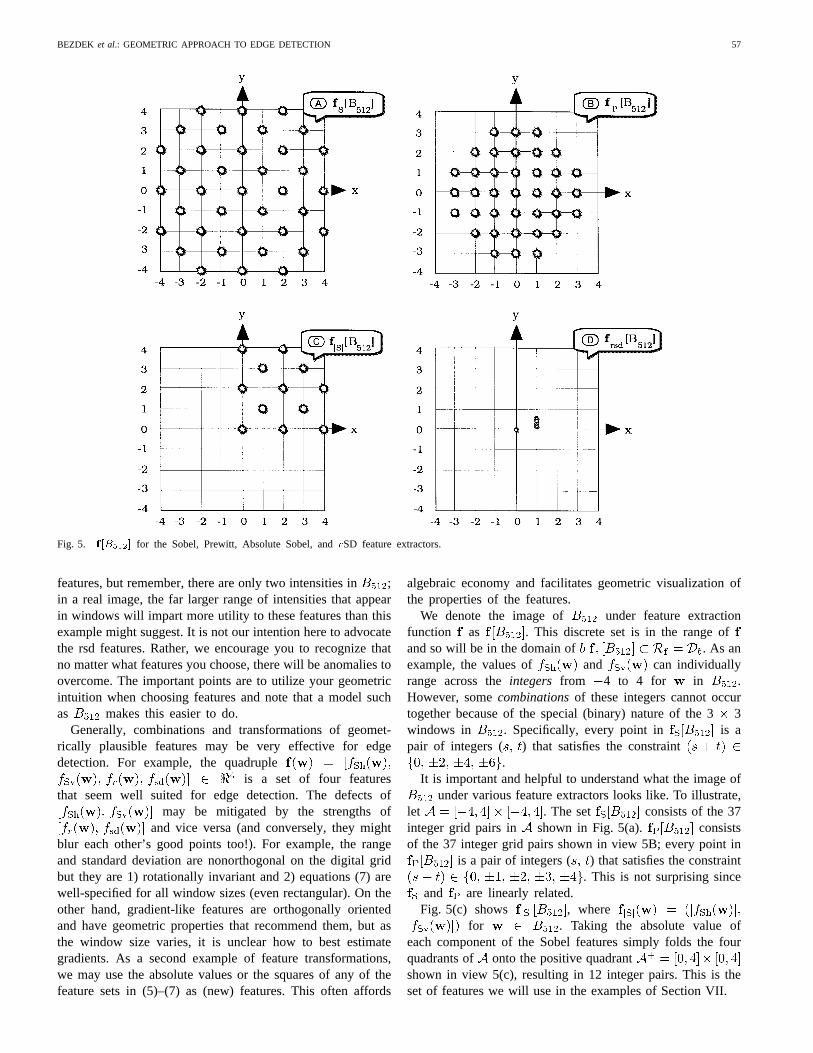
Fig. 5. f [B512] for the Sobel, Prewitt, Absolute Sobel, andrSD feature extractors.

features, but remember, there are only two intensities in ;in a real image, the far larger range of intensities that appearin windows will impart more utility to these features than thisexample might suggest. It is not our intention here to advocatethe rsd features. Rather, we encourage you to recognize thatno matter what features you choose, there will be anomalies toovercome. The important points are to utilize your geometricintuition when choosing features and note that a model suchas makes this easier to do.

Generally, combinations and transformations of geomet-rically plausible features may be very effective for edgedetection. For example, the quadruple

is a set of four featuresthat seem well suited for edge detection. The defects of

may be mitigated by the strengths ofand vice versa (and conversely, they might

blur each other’s good points too!). For example, the rangeand standard deviation are nonorthogonal on the digital gridbut they are 1) rotationally invariant and 2) equations (7) arewell-specified for all window sizes (even rectangular). On theother hand, gradient-like features are orthogonally orientedand have geometric properties that recommend them, but asthe window size varies, it is unclear how to best estimategradients. As a second example of feature transformations,we may use the absolute values or the squares of any of thefeature sets in (5)–(7) as (new) features. This often affords

algebraic economy and facilitates geometric visualization ofthe properties of the features.

We denote the image of under feature extractionfunction as . This discrete set is in the range ofand so will be in the domain of . As anexample, the values of and can individuallyrange across theintegers from 4 to 4 for in .However, somecombinationsof these integers cannot occurtogether because of the special (binary) nature of the 33windows in . Specifically, every point in is apair of integers ( ) that satisfies the constraint

.It is important and helpful to understand what the image of

under various feature extractors looks like. To illustrate,let . The set consists of the 37integer grid pairs in shown in Fig. 5(a). consistsof the 37 integer grid pairs shown in view 5B; every point in

is a pair of integers ( ) that satisfies the constraint. This is not surprising since

and are linearly related.Fig. 5(c) shows , where

for . Taking the absolute value ofeach component of the Sobel features simply folds the fourquadrants of onto the positive quadrantshown in view 5(c), resulting in 12 integer pairs. This is theset of features we will use in the examples of Section VII.


(a) (b)

Fig. 6. The surfacesGk�k = f(x; kxk1) jx 2 Ag and Gk�k = f(x; kxk2) jx 2 Ag.

The set is shown in view 5(d). Letting anddenote the number of ones and zeros in, it is easy to checkthat for , and the range of

is either zero or one. Consequently, all windows with (zeroor nine), (one or eight), (two or seven), (three or six), and (fouror five) ones, map, respectively, to the feature pairs (0, 0), (1,0.3143) , (1, 0.4157) , (1, 0.4714) , and (1, 0.4969). Thispaucity of input pairs may make thesd features inadequatefor training inputs to models that use learning algorithms asblending functions, but again, there are only two intensitiesin compared to a far larger range of intensities in a realimage.

Fig. 5 illustrates another important point about using a basisset such as for training. As the function changes, thecoverage by of some base set such asin Fig. 5 doestoo. This can have a dramatic effect on the approximationquality of the learning model being trained. It is difficult tosee (visually) that contains only five distinct pairsfor all 512 windows in : it is plotted on at the samescale as the other three views so you can see how nonuniformly

is covered under different choices for.

V. BLENDING FUNCTIONS (b)

Once features are chosen, we must pick theblending func-tion , which aggregatesthe information about edges possessed by for the purposeof edge detection. There are many types of blending functions.Of these, we discuss three parametric families: 1)norms, ofwhich the two most common families are the inner productand Minkowski norms; 2) generalized logistic functions; and3) computational learning models such as neural networks andfuzzy systems.

A. Norms

Let be any positive definite matrix. For

(8)

is the inner product norminduced on by weight matrix. Equation (8) defines an infinite family of norms on

parametrized in , the most important being the Euclideannorm which is induced by , the identity matrix

(9)

A second infinite family of norms that can be used forblending are theMinkowski norms, parametrized in

(10)

The three most commonly used in practice are the one, two,and sup norms

City Block (11a)

Euclidean

(11b)

and

Sup or Max (11c)

For convenience, we let andwhere is any norm on . When needed, we

may indicate the parameter of each of the families in (8) and(10) explicitly as and

, respectively. The Euclidean normof the components of is often regarded as the standardblending function, but there is no reasona priori to preferthe Euclidean norm of, for example, the Sobel featuresas the best way to make Sobel edge images. The importantpoint is thatany norm can used to combine the componentsof . Fig. 6(a) and (b) shows the graphs of the one andtwo norms on .

Viewing the blending function this way gives much insightinto the properties of different edge operators. We see inFig. 6(a) that the surface defined by the one norm is a conewith flat sides that are radially symmetric (in the sense of


(a) (b)

Fig. 7. The surfacesGb (x; k�k ; �; 0:1) on A for (a) � = 10 and (b) � = 1.

the one norm) about the axis. Level sets of this surface arediamonds in the ( ) plane centered at the origin. Similarly,the two norm generates a cone over with circular levelsets in the ( ) plane. The graph of every norm on anyfeature space has a similar shape—it “holds water”—becauseall norms on are convex functions. Consequently, a linesegment such as in Fig. 6(b) connecting any pair of pointsin the graph of any norm will liein or above the surface.Our experience is that this shape for the graph of the blendingfunction is not particularly favorable for the detection of edges.We contend that blending functions that areconcave, at leastlocally in the neighborhood of the origin, can lead to betteredge images than norm functions. The next family of blendingfunctions we discuss has this property.

B. Waterfall Functions

Blending functions that arenearly concave(instead ofconvex) in the neighborhood of the originin feature spacewill be called waterfall functions, in analogy with the shapepossessed by a profile view of a typical waterfall (i.e., they“shed water”). We do not give a mathematical definition ofnearly concave, preferring instead to simply tell you whattype of graphs we want. Generalizedlogistic functionsin the

arguments of

(12)

where is again any norm on and are realpositive constants can be locally concave or convex near zeroin . is an infinite family of three parameter blendingfunctions whose general shape is affected more by (, )than by the norm used in (12). For example, with the twonorm and fixed, varying in (12) produces a familyof surfaces that range from an extremely “punctured” shape(large values of ) such as is seen in Fig. 7(a) ( )that is locally concave near zero to surfaces that are locallyconvex near zero and, hence, resemble the graph of theinducing norm such as seen in Fig. 7(b) ( ). Since

for any choice ofparameters in (12), none of these functions takes the value zeroat the origin. This is evident in Fig. 7, where you can see thatthe vertical scale in both plots starts above zero. In particular,

and. Consequently, cannotbe zero on the window in

Fig. 4. Since the value is interpreted as the extent towhich should be regarded as possessing an edge, this mayseem counter-intuitive. However, we think that the responseof at the origin is less important than the changein responsefor ’s near zero. Waterfall functions give large (more thanlinear) response to small changes near zero, whereas convexfunctions give lower increments in this neighborhood.

Fig. 8 shows the piece of the surface in Fig. 7(a) on [0, 1][0, 1]. You can see why we call this a waterfall function. Noticetwo things. First, has essentially attainedits asymptotic limit of one for vectors lyingbeyond the circle . For example, thevalue at (0.5, 0.0) is 0.982, so only feature vectors near theorigin will provide sharp differential edge response. Second,this surface appears to be concave along the axes of its domainand convex perpendicular to the line near the origin,so it is neither convex nor concave in this region. This is notby intention, but we point it out to make sure that you seethe important point about waterfall functions: we think that

should be large when is close tozero and experiences a relatively small change.

C. Learning Models

The last type of blending functions discussed here arecomputational transformations(input–output systems) such asneural-like networks[18] and theTakagi–Sugeno(TS) fuzzyreasoning model [19]. Both of these schemes are well knownfor their ability to provide good approximations to ratherarbitrary nonlinear vector fields. In the present context, theycan be used effectively to blend vectorial inputs such asin , and can be either trained or subjectively configured toproduce good edge values at their output layers. We denotethese two cases as and . Learning models requiretraining data, and in particular, we need to know what “goodedge output values” are for inputs such as . To ourknowledge only two previous studies use model-based trainingdata (viz., ) for an edge detecting feed forward neuralnetwork [10] and for the TS model [16]. Here, weextend this idea to a much more general scheme that depends


Fig. 8. The surface generated bybL (x; k � k2; 10; 0:1) on [0, 1] � [0, 1].

explicitly on knowledge of the graph of thedesiredblendingfunction. Specifically, are the targetoutput scores on the training inputs . The desired(target) outputs are found by specifying and and thenapplying to . This gives a set of IO pairs, say

that can be used to traincomputational learning models for edge detection.

More generally, we letto emphasize that there are three components to building: 1) themodel basis set ; 2) thefeature extraction function

; and 3) theblending function . Changingany of thesethree will change and also the edge detectorsubsequently trained with it. We expect the trained mapping todetect edges because 1) the window vectors are chosenselectively to reveal edges; 2) the features are chosenbecause they are related to geometric properties of edges; and3) the blending function () is chosen so that its graph has ashape that is maximally responsive to the perception of edges.

Fig. 9 illustrates the construction of . The model basis isa box B containing the chosen set of window vectors .The horizontal plane represents , the chosen feature space.Choosing determines the dimension, and knowing the setof gray levels fixes . The training inputs willbe a discrete subset in the domain of, , asshown in Fig. 9. For example, any of the discrete sets(or combinations thereof) shown in Fig. 5 could appear asin Fig. 9. The target outputs are simply the values ofon .It is here that knowledge of the desired shape of the blendingfunction comes into play. Analytically expressed blendingfunctions such as norms or generalized logistic functionsare simply evaluated on . Alternatively, any method of

specification of the values completes .(Some authors have scored windows completely “by eye” andhave reported reasonable results [7].) After training, or

becomes the blending function.If we wanted to approximate the surface over , we

would probably choose a nicely arranged lattice of base pointsin . Typically, such a lattice is rectangular and gridspacing is chosen small enough to insure that the training dataprovide a reasonable sample for fitting a surface to the pointschosen. For edge detection, however, the input training pointsare chosen as points in that possess edge information; thatis, points in . Fig. 5 shows that these points may or maynot cover the domain of in a nice way from the standpointof numerical analysis or from the standpoint of training andtesting in pattern recognition. But from the standpoint of edgedetection, we believe that very few points are actually needed,provided they are related to edge geometry, the shape of theblending surface is correct and at least some of the points areconcentrated near the origin.

D. The Takagi–Sugeno (TS) Model

As a specific example of the ideas in Section V-C, wediscuss the TS model, which is a fuzzy rule-based inferenceengine that can be used for function approximation. Themultiple-input single-output (MISO) case is summarized inFig. 10. In step in is an inputvector.

Step begins with the identification of the numerical rangeof each input variable. For each, the numerical domainis found and associated with alinguistic variable thatprovides a semantic description of () subdomains of .


Fig. 9. The three elements ofTIO(B; f ; b).

Fig. 10. The general architecture of the TS model.

The number () is called thegranularity of ; generally,can be a function of . The th subdomain of represents

a linguistic value, say . This linguistic value is in turnrepresented by a fuzzy membership function

. In Fig. 10, the membership functions all have symmetrictriangular graphs, but again, this need not be the case. The set

is called thelinguistic termsetassociatedwith variable , . Step is often referred to asfuzzificationof the input domain.

Step comprises the reasoning mechanism. The left-handside (LHS) and right-hand side (RHS) of therule base(RB)are composed of rules that operate on and takethe general form

(13a)

(13b)

(13c)

In (13b), is called thefiring strengthofrule . Here, is any -norm (intersection)operator [20] on [0, 1] [0, 1]. Our notation is a littlesloppy, because is not the value of a fixed vector field

on . Instead, the membership functions that yield thearguments of depend on the input . In other words,


different membership functions among the will be usedas runs through its domain.

The output functions comprise the RHS ofthe rule base. Each has a functional form (e.g., linear, affine,quadratic, polynomial, trigonometric, transcendental, power,etc.) specified by the user. It is common, but not necessary,to require that all the ’s have the same functional form.Step produces the numerical output by combining thefiring strengths and outputs of the individual rules with someaggregation operator . Usually, is taken as the weightedsum

(14)

If any component in rule (say the th) is zero; then. This means that a

given input vector in will probably never fire all of therules in (13)—most of the will be zero. If care is takenduring fuzzification, it will never happen thatall of the firingstrengths are zero. Consequently, the system is well definedand can be constrained to have an output that always lies ina specified range .

We can summarize (13) and (14) succinctly by noting thatis simply a mapping. This is entirely analogous

to a computational neural network in that the function TS isspecified by a computer program (as opposed to a functionin closed form). Analogous to Kolmogorov’s theorem forthree-layer feed forward neural networks, there are many“universal approximation” theorems that give conditions underwhich mapping TS exactly represents continuous functions oncompact subsets of [20].

Suppose that each in (13) is parametrized by an unknownset of parameters in a parameter space . Assuming thatall other choices and parameters for the TS model in Fig. 10are fixed, completion of the model means acquiring “goodvalues” for the parameters . There aremany ways to do this, partially dependent on the form of theoutput functions. When the ’s are all affine (linear plus aconstant), we call the system afirst-order TS model; eachoutput function can be written as a Euclidean dot product in

, , whereand . In this case, Takagi andSugeno [19] show how to find a minimizing least-squared error(LSE) solution to a (possibly rectangular) linear system formedby submitting IO pairs , ; , tothe TS model. This method uses the psuedo-inverse to findthe LSE solution and, as grows, it becomes more andmore intractable numerically because the matrix of coefficientsis usually quite sparse (not many rules fire for each input

). Alternatives to this method that generalize well to morecomplicated types of output functions include gradient descent[21] and neural networks [22].

For some feature extraction and blending functions, itis possible to solve the LSE problem associated with theTS model analytically. Specifically, in [16] a 12-rule TSblending function, say , interpolates the training data

, which has also been used to train

Fig. 11. Membership functions onx = jfSh(w)j for the 12-rule blendingfunction bTS12.

a feed forward neural network edge detector having nineinput nodes, one output node, and two hidden layers ofseven and two nodes [10]. The resultant blending function

was reasonably successful at detecting edges in variousreal images. Fig. 11 shows the linguistic termset and itsmembership functions for . The coordinate

used the same set of functions. There aremembership functions over each of and . The linguisticvariable for both inputs is “quantity,” and the linguistic valuestaken by the inputs are:low L; medium-low ML; medium

M; medium-high MH; and high H.Each of the membership functions for and shown in

Fig. 11 has the convenient representation

(15)

where is the positive slope of the leading edge line, andis the center of the nonzero portion of the graph (the point

at which ). For the case shown, the slopes are allone and the center of each function is set at one of the integersin . For example, for a given input vector , thelinguistic statement “ is medium” is represented by the value

.

E. Using the Takagi–Sugeno Model without Training

Now we discusssubjective designas done in [11]–[15].First, choose two semantic terms and membership functionsalong the and axes. The two membership functions foreach input variable must still cover the numerical domain ofthe chosen features, which is [0, 4] for where

and .Fig. 12 shows membership functions for “low” and “high”

(on and ) for a four-rule TS model that represents theblending function we call . Rather thantrain this modelwith some , we specify output functions for

that make it a four parameter family of models. Letand define the rules as

R1. If and (16a)

R2. If and (16b)

R3. If and (16c)

R4. If and (16d)

System (16), with the functions shown in Fig. 12, is aregular first-order TS model when ; and otherwise, itis regular but neither linear nor polynomial (unlessis aninteger). Now we choose the norm as the product of itsarguments, . The functions in Fig. 12 satisfy


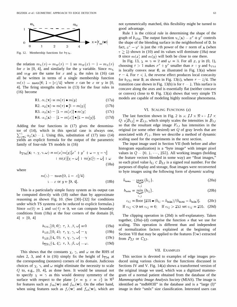
Fig. 12. Membership functions forbTS4.

the relation sofor in [0, 4], and similarly for the variable. Sinceand are the same for and , the rules in (16) canall be written in terms of a single membership function

where can be or in [0,4]. The firing strengths shown in (13) for the four rules in(16) become

R1. (17a)

R2. (17b)

R3. (17c)

R4. (17d)

Adding the four functions in (17) gives the denomina-tor of (14), which in this special case is always one,

. Using this, substitution of (17) into (14)yields an explicit formula for the output of the parametricfamily of four-rule TS models in (16)

(18a)

where

or (18b)

This is a particularly simple fuzzy system as its output canbe computed directly with (18) rather than by approximatereasoning as shown Fig. 10. (See [30]–[32] for conditionsunder which TS systems can be reduced to explicit formulas.)Since and , we can compute boundaryconditions from (18a) at the four corners of the domain [0,4] [0, 4]

(19a)

(19b)

(19c)

(19d)

This shows that the constants, , and on the RHS ofrules 2, 3, and 4 in (16) simply fix the height of atthe corresponding (nonzero) corners of its domain. Judiciouschoices of , , and might eliminate the necessity to scale

to, e.g., [0, 4], as done here. It would be unusual notto specify as this would destroy symmetry of thesurface with respect to the plane infor features such as and . On the other hand,when using features such as and , which are

not symmetrically matched, this flexibility might be turned togood advantage.

Rule 1 is the critical rule in determining the shape of thegraph of . The output function controlsthe shape of the blending surface in the neighborhood of. Infact, is just the th power of the norm of (when

) shown in (10) and its values will dominate (18a) nearsince and will both be close to one there.In Fig. 13, and . For all in (0, 1),

choosing makes smaller than andis locally convex near , as illustrated in Fig. 13(a) where

. For , the reverse effect produces local concavityfor near , as shown in Fig. 13(c), where . Thetransition case shown in Fig. 13(b) is for . This surface isconcave along the axes and is essentially flat (neither concaveor convex) close to . Fig. 13(a) shows that very simple TSmodels are capable of modeling highly nonlinear phenomena.

VI. SCALING FUNCTIONS ( )

The last function shown in Fig. 2 is, which simply scales the intensities in

so that the resultant edge image has intensities in theoriginal (or some other desired) set of gray levels that areassociated with . Here we describe a method of dynamicscaling used for the experiments in the next section.

The input image used in Section VII (both before and afterhistogram equalization) is a “byte image” with integer pixelvalues in . All working images (holdingthe feature vectors blended in some way) are “float images,”so each pixel value is a signed real number. For thepurposes of display and storage, float images were reconvertedto byte images using the following form ofdynamic scaling

(20a)

(20b)

floor (20c)

If set If set (20d)

The clipping operation in (20d) is self-explanatory. Takentogether, (20a)–(d) comprise the functionthat we use forscaling. This operation is different than and independentof normalization factors explained at the beginning ofSection VII that may be applied to the features extractedfrom or .

VII. EXAMPLES

This section is devoted to examples of edge images pro-duced using various choices for the functions discussed inSections IV and V. Fig. 14(a) shows a transformed version ofthe original image we used, which was a digitized mammo-gram of a normal patient obtained from the database of theMammographic Image Analysis Society(MIAS). The image isidentified as “mdb003ll” in the database and is a “large (l)”image in their “smlx” size classification. Interested users can


(a) (b)

(c)

Fig. 13. Three surfaces generated bybTS4 on [0, 4] � [0, 4]. (a) � = 4. (b) � = 1. (c) � = 0:25.

obtain further information on the database from the MIAS website or by e-mailing the MIAS [23].

The original image (called in Section II) was scannedat 50 ’s per pixel in each of the two orthogonal directionsby a scanning densitometer that maps the optical density[log (incident light intensity/transmitted light intensity)] toan eight bit number (0–255) at each pixel. The originalimage size was by . We reduced theoriginal image to 163 (rounded up from 162.5) by 270 pixels(44 010 pixels) at a resolution of 800’s per pixel in eachdirection, by successively averaging 8 8 neighborhoodsof the original image followed by a second compression of2 2 neighborhoods. This operation was not discussed inSection III, but is a conditioning operation that results in theimage in Fig. 14(a). To be consistent, the image in view 14(a)should not be called ; we have done so here to simplifythe figure captions.

Following size reduction, we applied the histogram equal-ization in (4) to image Fig. 14(a), resulting in the conditionedimage we call in view 14(b). Edges in image14(b) have more acuity than those in view 14(a), making visualcomparisons with edge images somewhat easier. At the otherend of the processing sequence is scaling, represented here asthe function specified by (20). Most of the edge operatorswe examine have the general form , theexception being experiment 7.2, which studies itself.

There are some key elements in Fig. 14(b) that we willallude to when comparing different outputs. First, there is themain boundary (or skinline) of the breast and the milky web-like structure within it. Second, there is a very slight area(noise spot) introduced by (4) of just a few pixels to the rightof the main boundary and to the left of the number 19. Finally,there is the label box in the upper right-hand corner thatsurrounds the letters ML. These reference points are especiallyuseful for visual comparisons of different edge images.

Edge images will be discussed that use various combinationsof the features . Here,is a vector of nine intensities from any 3 3 window in

, each value of which in the real image can be anyinteger in . The absolute Sobel features areused here as a convenience: their utility as edge detectionfeatures is not importantly different from the signed features

.Fig. 5 shows that different features attain different max-

imum values on the same window. To facilitate unbiasedblending of various features, it seems desirable tonormalizethem to a standard range. There are many normalizations. Forexample, when images have 256 gray levels, we can normalizethe absolute Sobel features to the range [0, 255] by division by4 to agree with the natural range of thesd features. Here, wechoose to normalize all features to be real numbers lying inthe closed interval [0, 4]. This means that the absolute values


Fig. 14. A (compressed) digitized mammogram and its histogram equalization by (4).

of the Sobel features are divided by 255,by 63.75 andsd by 31.68, respectively.We, henceforth, refer to these fournormalized features as and (not sd), respectively.

The remaining pages of this section discuss various aspectsof edge images produced from . There is no “gold stan-dard” or ground truth edge image that can be used to comparevarious outputs. Heathet al., [24] advocate an interesting andmore rigorous approach to this problem than the usual one(which is to look at them) based on human ratings experiments.Here, we resort to the usual method of side by side visualassessment to compare the efficacy of different models. Beforereading our discussion about these images, page through thefigures in this section and form your own opinions about theirrelative visual qualities. For fun, rank the outputs and compareyour rankings to ours. Obviously, you may not agree with us,but this exercise may provide you with a little relief from theeffort of struggling through the tortuous path that has broughtyou this far.

Experiment 7.1. Different Features:Fig. 15 shows eightedge images produced by . The onlyvariable in Fig. 15 is —the feature extractor function.

First, compare Fig. 15(a)–(d). These four views are madewith just one of the four features or . All visibleedges of the label box are clearly found using eitheror. On the other hand, (the normalized absolute horizontal

Sobel feature) misses the vertical edges of this box, whileits counterpart misses the horizontal edge of the box. Thisis expected based on the geometrical meaning of these twofeatures. By contrast, either or both provide clear edgesin both directions, emphasizing their nondirectional geometricnature.

Fig. 15(c) best shows the structure within the breast that isseen in Fig. 14(b) and, overall, we think it the best of these four

views. Gonzalez and Woods state that “the idea underlyingmost edge-detection techniques is the computation of a localderivative operator” [17, p. 416]. Fig. 15(c) and (d) shows thatother kinds of features can also be used to produce good edgeimages.

Fig. 15(e) and (f) are made with the feature pairs ()and ( ). Edges in Fig. 15(e) appear somewhat thinner thanthose in Fig. 15(f) and, as expected, the use of bothand

enables this detector to find all the edges of the ML labelbox. On the other hand, Fig. 15(f) possesses somewhat morestructure within the breast and has somewhat better contrast.The principal difference between these two views can be seenby comparing the letters ML in the label box and the noisepixels in the far right of each view. The gradient-based features( ) produce an “edgier” visual effect than the statistically-based ( ) feature pair. Overall, these two images are reallypretty similar.

Panels g and f in Fig. 15 show edge images produced byusing the triple ( ) and the whole set ( ). Thebest way to assess each of these views may be to compare eachof them to Fig. 15(e), which is the edge image correspondingto ( ) alone. Adding the standard deviationto ( ) asin Fig. 15(g) yields an image that is visually brighter; that is,

seems to enhance contrast, but this image is somewhat moreblurred than Fig. 15(e). Adding ( ) to ( ) as in Fig. 15(f)gives a result much like Fig. 15(g). All views that usedor

or both produce a more visible noise spot; none of the eightviews shows the number 19 well.

We examined many edge images using these and othercombinations of features with various blending functions.In many cases, the results were similar, but there were al-ways small and possibly important differences. Fig. 15 shouldconvince you that using nonstandard features as well as


Fig. 15. (a)–(d) Different features using the two norm for blending.

combinations of features such as these—with ANY blendingfunction—may give a result that is better (that is, more usefulfor the application at hand) than those based on the traditionalderivative-like features mentioned by Gonzalez and Woods.Which of these eight views did you rate best? We choseFig. 15(c), followed by Fig. 15(e) as the second best view.

Experiment 7.2. Different Norm-Based Blending Functionsand Scaling:This experiment has two objectives—to comparedifferent norms for using the features ( ) and ( )

and to see the effects of dynamic scaling as done by (20) onimages produced by the sequence .

Equations (8) and (10) provide two norm families parame-trized in and . The most obvious candidate from family(8) besides the Euclidean norm at (9) is the Mahalonobisnorm induced by the inverse of the covariance matrix of ,

cov . However, since the Euclidean norm isalso in family (10), we chose to illustrate only the one, two,and sup norms in this example.


Fig. 15. (Continued.)(e)–(h) Different features using the two norm for blending.

Fig. 16 shows four edge images [views (a), (b), (e), and(f)] before dynamic scaling corresponding to

, where ( ) is a constant scale factor chosenso that the one norm would just saturate at 255; and fouredge images [views (c), (d), (g), and (h)] after scaling, corre-sponding to . We use theMinkowski norms for at (11a) and at (11c) asblending functions. Viewing Fig. 16 in conjunction with partsof Fig. 15 also enables you to compare these two norms withthe more familiar Euclidean norm at (11b). In this and

subsequent figures, 1, 2 , and sup stand for the 1, 2,and sup norms.

Fig. 16(a) and (b) are without scaling and do not have acompanion view for the two-norm in Fig. 15. Fig. 16(c) and(d) use the same parameters as Fig. 16(a) and (b), but withdynamic scaling as described in (20). Fig. 15(e) “fits between”these two views as it also uses ( ), the two-norm, and

. As in (10) increases from one to infinity, edge imagesproduced using (10) for blending become darker and seem tolose definition without dynamic scaling. In contrast, there are


Fig. 16. (a)–(d) Norm blending using (h; v) before and after scaling.

only slight differences between Figs. 16(c), 15(e), and 16(d),corresponding to scaled edge images using the one, two, andsup norms, respectively.

Fig. 16(e)–(h) shows four images with the same scaling andblending functions as 16(a)–(d) using the statistical features( ) instead of the normalized absolute Sobel pair ().First, compare the four views 16(e)–(h) to the correspondingviews in 16(a)–(d) panel by panel. Using ( ) brightensall four images and again thickens both edges and noise tosome extent. The contrast between the one and sup norms

as blending functions is seen more easily in Fig. 16(e) and(f) than in Fig. 16(a) and (b): as increases, brightness anddefinition are lost. But we see again in Fig. 16(g) and (h) thatscaling essentially removes this difference. Finally, Fig. 15(f)“fits between” these two views as it also uses (), thetwo-norm, and .

Looking at the before and after views in Fig. 16 shows twothings: dynamic scaling enhances edges in the unscaled ver-sions and scaling by (20) also decreases apparent differencesin edge quality due to different-norm blending functions.


Fig. 16. (Continued.)(e)–(h) Norm blending using (r; s) before and after scaling.

An infinite set of edge images can be generated in this waythat will be (digitally) continuous in their change from viewto view as runs from one to infinity in (10). It is NOT thecase, as asserted in [17, p. 418], that the length of the vector( ) in the one-norm is simply an approximation to its lengthin the two-norm. Every norm gives an equally valid measureof the length of vector ( ). Mathematically, all norms areadmissible and, operationally, it is clearly the case that varyingthis kind of blending function with all other components of the

sequence fixed will result in a wide variety of edge images ifcare is not taken to use a form of scaling that puts them all onthe same relative footing. But if scaling is used appropriately,there seems to be only slight differences in the resultant edgeimages, so ease of computation might be an important factorin your choice of norm. Which image in Fig. 16 seems mostappealing to you? Our pick is Fig. 16(g).

Experiment 7.3. Different Generalized Logistic BlendingFunctions: Fig. 17 shows eight edge images corresponding


Fig. 17. (a)–(d) Logistic blending functions with� = 10 and � = 0:5 using (h; v) and (r; s).

to . The images in thisseries use logistic functions as in (12) for blending. Thereare three parameters for , so it is impossible to showthe wide variety of edge images that can be realized as eachparameter is varied. Fig. 17 shows a few representative imagesobtained with this family that enable us to study several facetsof logistic blending functions. Fig. 17(a)–(d) compare edgeimages obtained with and fixed while the norm andfeatures vary. Fig. 17(e)–(h) show images corresponding to afixed norm and features while and vary.

The only difference between Fig. 17(a) and (b) is the normused in (12). The one-norm seems to result in somewhatbrighter and thicker edges, and the internal structure of thebreast is slightly more well-defined than when the two-normis used. Fig. 17(c) and (d) show the results of using the ()feature pair instead of ( ) with all other parameters ofFig. 17(a) and (b) fixed.

All four images in Fig. 17(a)–(d) based on logistic blendingshow more internal structure and thicker edges than previousviews based on blending with norms and are, in some loose


Fig. 17. (Continued.)(e)–(h) Logistic blending functions using (h; v) and the one-norm:� versus�.

sense, “in-between” edge and region segmentations of theimage. The ( ) features reveal many more edges thanthe normalized Sobel gradients, and the internal structure ofthe breast is very detailed (refer to Fig. 14(b) for a visualbenchmark). And, as in previous figures, () continues togive brighter and thicker edges than ( ).

The dependency of on and can be seen inFig. 17(e)–(h) in which ( ) and the one-norm in (12) arefixed. Fig. 17(e)–(g) hold fixed while varies from

100 to 10 to 5. Changing has a very pronounced effect onthe output. Recall that all images in Fig. 17 are dynamicallyscaled via (20), so the transition from almost monochromaticat to very gray at is directly attributable tothe value selected for . If we plot as a function of thenorm on [0, 4] with and as parameters, we get a seriesof curves reminiscent of the transfer characteristics of digitalswitches that switch from one state to another. Parametercontrols the value of the input ( ) at which the transition


occurs, while controls the suddenness or steepness of thetransition. When , the transition or switching occursalmost at once and the result is a “digitized” edge image asin panel Fig. 17(e). For this value of, behaves as if itwere in a “saturation” mode analogous to a transistor switch;it functions as a thresholder and binarizes the image. When

as in Fig. 17(f), the transition is more gradual witha linear, intermediate region. As continues to decrease [seeFig. 17(g)], this effect continues until , at which theswitching behavior is entirely lost and we get “linear” modeswith “milky” images.

Finally, compare Fig. 17(f) and (h) (above and below onthe right side). The only difference between these two resultsis that in Fig. 17(f), whereas its value in Fig. 17(h) isone. This shows how can be used to create a range of edgeimages that appear very gray (small values of) to essentiallyblack and white (large values of). The value of governswhen the onset of transition occurs. If is large [1 or 2, forexample, as in Fig. 17(h)], most of the low-intensity edges willbe switched out with the result that only the strong edges willshow in the final, dynamically scaled image. Makingsmall[close to zero as in Fig. 17(f)] allows the whole dynamic rangeof the edge image to be subjected to the sigmoidal modulationof the logistic function. This results in a detail-rich edge imagewhose appearance depends on(crisp black and white ifis large, and milky if is small). If is made very smalland we are in saturation mode, we can get a binary image thatroughly segments the breast and background in mammograms.Conversely large in saturation mode can lead to a totallyblack image with no information. By choosing and sothat operates in the linear mode, we can get an image withthe degree of edge detail we desire.

When viewing the panels in Fig. 17, it is useful to rememberthat for fixed features as in six of the eight Fig. 17 views,variations in the three parameters of changethe shape of the graph of the blending surface correspondingto a particular function. Fig. 17 shows that logistic blendingfunctions provide a very rich family of edge detectors thatyield an almost infinite variety of edge images. The underlyingmathematical reason for this lies with the shape of the graphsthat correspond to different members of the blending functionfamily. Incidentally, we would, as with previous figures,certainly call all of the images in Fig. 17 that use the ()feature pairSobel edge images. Which of these images do youprefer? For this example, it is hard to choose, because thereare really several types of images. Our pick for the best edgedefinition is Fig. 17(a), and the best internal structure seemsto be in Fig. 17(f).

Experiment 7.4. Different TS Blending Functions:Fig. 18shows six edge images for .There are four parameters for , so it is again impossibleto show the wide variety of edge images that can be realizedas each of these is varied. To study our contention that thebehavior of the TS4 blending function near the origin is moreimportant than elsewhere, we study variation in e usingonly as a function of in (18a) and the features it blendstogether. Panels (a), (b), and (c) in Fig. 18 use the absoluteSobel features ( ), whereas views (d), (e), and (f) use the

( ) pair. Each vertical block uses the same choices for,so this affords a third comparison of edge image quality as afunction of extracted features. The images in this series are alldynamically scaled with (20).

Fig. 18(a)–(c) [and also Fig. 18(d)–(f)] correspond to theTS4 blending functions having the shapes of the three surfacesshown in Fig. 13(a)–(c), respectively. In particular, for[Fig. 18(a) and (d)] the blending function has the graph shownin Fig. 13(a)—that is, is locally convex. Because thisblending function shape is locally similar to the two-norm (thefour norm would make a better comparison, but we have notshown images in Fig. 15 and 16 for the 4 norm), this pair ofimages is best compared to Fig. 15(e) and (f), the analogousedge images produced on these two feature sets with the two-norm as the blending function. There, as here, the edge imageslack contrast and structural detail; and in both places, the ()feature pair seems to produce brighter, thicker edges.

The middle two frames, Fig. 18(b) and (e) for showedge images that are best compared to Fig. 16(c) and (g),respectively, both of which use the one-norm. Match Fig. 16(c)to 18(b): we think that Fig. 18(b) is much brighter and morestructurally detailed. Now compare Fig. 16(g) to 18(e); again,the TS4 image appears quite superior to its counterpart usingthe one-norm for blending. In our opinion, Fig. 18(b) is a muchcrisper and more detailed edge image than any shown so far.Fig. 18(c) and (f) shows the result for with the twofeature pairs. At this value of the graph of ramps upquite steeply (perhapstoo steeply for goodedge detection)for feature vectors near . This pair of images are mostcomparable visually to the milky, segmentation-like outputsproduced by the logistic function—Fig. 17(f) for example.

Comparing views in Fig. 18(a)–(c) [or Fig. 18(d)–(f)] im-parts the striking effect that variation in the shape of thegraph of the blending function near the origin can have as

progresses from 4 to 1/4. Moreover, this also shows thatthe TS4 edge detector, like logistic blending functions, canproduce a wide and richly diverse variety of edge images asa function of its parameters. The image in Fig. 18(e) mightbe useful for detection of the skinline, whereas the image inFig. 18(f) might find applications in the characterization anddetection of mass lesions. Views in Fig. 18(e) and (f) are ourchoices for the most visually informative images in this series.Which did you pick?

VIII. C ONCLUSIONS AND DISCUSSION

We have made and will briefly discuss six points, viz.:

1) viewing edge detection via the architecture shown inFig. 2 clarifies the role of each part of the edge detectionprocess;

2) good features for edge detection need not be digitalgradients but may be statistical, etc.;

3) a small basis set of windows may clarify feature per-formance and are essential for training computationallearning models for edge detection;

4) a proper match between the desired features of the edgedetector and the graph of the blending function leads to(visually) optimal edge images;


Fig. 18. TS4 blending functions using (h; v) or (r; s) with � = = 2 and ! = 3.

5) blending functions whose graphs have the (loosely char-acterized) waterfall function shape may provide betteredge response than norms;

6) parametric families of blending functions such as thegeneralized logistic functions and the Takagi–Sugenomodel provide a means for generating a richly diverseset of edge images through control of simple parame-ters.

The first point we emphasize is that our architecture clarifiesthe role played by the features in edge detection models. The

Sobel masks in (5) produce edge related features which arefixed in valuefor a given image. Our decomposition of thedetection process makes it clear that there is not just one Sobeledge image, but infinitely many. It is entirely proper, in ourview, to call every image in Fig. 15–18 that are based entirelyon or or ( ) a Sobel edge image. There are as manydifferent Sobel images as you care to construct and they mayhave very different visual appearances and utility.

Another important point that has been made is that thefeatures chosen need not be entirely composed of estimates of


digital gradients. Gradient-like features based on the geometryof derivatives have three important properties (direction ofmaximum rate of change, maximum magnitude of the change,and digital orthogonality) for edge detection. Our exampleshave shown that the range and standard deviation of pixelintensities in can serve equally well, and in some cases,better than estimates of digital gradients.sd features havefour important properties that complement digital gradients:they are rotationally invariant, nonorthogonal, invariant (infunctional form) to window size, and have well known sta-tistical distributions. We have also shown that there is nogood reason to constrain the search for edge features to 2-Dderivative-based vectors and there is noa priori reason notto try combinations of various features, as long as each pos-sesses edge detecting capabilities via its geometric meaning.Moreover, the analysis of features that may or may not beuseful for edge detection is greatly enhanced by using asmall and easily understood set of basis windows such as

.Once the features are chosen, we argued that the choice

of a blending function should not rest mainly with historicalprecedent or computational convenience. We have exhibitedthree families of blending functions that all produce viableedge images. We believe that the key to designing a usefuledge detector for a particular application should begin with acareful analysis of desirable properties of the edge image andsubsequent choice of an appropriate blending function. Howto do this for more than two features is an open question.Another interesting problem that deserves future research is acareful mathematical specification of the properties that makea blending function have a waterfall surface.

Another important step taken in this paper was to showhow to use fuzzy input–output rule-based systems such as theTakagi–Sugeno model for edge detection; papers [11]–[15] alluse the Mamdani [20] fuzzy system. This can be done in oneof three ways: 1) byspecificationof system parameters (aswe did for ); 2) by derivation of optimal coefficients (aswas done in [16] for ); or 3) by training a computationallearning model using (as was done in [10] for

). Further, we showed how the geometric approach couldbe used to get model-based IO training data that are needed forlearning when method 3) is used. There are many things thatcan be studied in connection with the TS model. For example,the configuration of the LHS of the rule base affects theedge response and offers something akin to compartmentalizedtuneability. The sensitivity of depends on the choice ofmembership functions for each linguistic variable. Althoughsymmetric triangular functions are convenient, it would beinteresting to study how to optimize the number (granularity)and shape of the membership functions that comprise thetermsets for each input variable. The firing strength of eachrule depends on the T-norm used for intersection. Here weused . There are seven infinite families of -norms andseveral families of averaging operators that can be usedinstead [20]. A change in this parameter clearly affects theedge image produced. The training set has obviousdrawbacks. can be enriched in a number of ways.For example, windows with values between zero and one

(0.5 corresponds to a gray level of 127) can be added toit.

The application domain hinted at by the examples in thispaper is the analysis of digital mammograms. Informationabout intensity, edges, texture, and shape plays a central rolein image segmentation and lesion detection in mammograms[25]–[28]. The results of this study are important to ourapplication in at least three ways.

1) Feature selection—edge and texture are generally re-garded as complementary properties of an image. Wehave shown in this study that the standard deviationof pixel values within a window—a traditional texturefeature—can function as a feature for edge detection aswell [33]. The judicious and economic choice of featuresthat embody “multiple dimensions of information” (suchas edge and texture) is vital to insightful characterizationand successful detection of lesions.

2) Adaptive blending of features—the need for local pro-cessing in lesion segmentation is well known [28], [29].Indeed, it is common for a single, continuous edge ina mammogram (such as the skinline of the breast) tovary in strength along its length [see for example, thebottom fifth of Fig. 15(e)]. A tuneable edge detector thatstrengthens weak edges without emphasizing strong onesis desirable for automatically extracting these edges.The parametrized analytical (logistic) and computational(TS4) blending function families introduced in this study(Figs. 17, 18) allow tuneable edge detectors to be de-signed systematically. Thus, one obvious application ofour results is to delineate the skin-air interface, thepectoral muscle boundary and the extent of the glandulartissue on a mammogram [Figs. 17(f), 18(c), 18(f)]. Suchblending functions are also ideal for blending intensity,edge and texture features adaptively to detect subtlemass lesions, for example.

3) Interactive optimization of diagnostic systems by practic-ing clinicians—an exciting possibility for computationalmammography is on-line tuning of digitally enhancedmammograms by practicing clinicians. Blending func-tions such as and offer a simple and convenientmeans for on-line visual optimization by adjustmentsto simple parameters of the functions. Thus, differentfeatures in an image can be enhanced in near real timeby simply “turning a dial.” We will be participating witha local hospital in experiments to ascertain the usefulnessof this idea in the near future.

Finally, it would be interesting to pursue the perceptualmechanism that underlies the cognitive process of edge detec-tion by humans implied by this study. It was our observationin this article that more than linear (waterfall) response toedge features near the origin of feature space coupled witha flat response far from seemed to produce visually betteredge images than norms (which have less than linear responsenear and which increase monotonically as feature vectorsget further from the origin). Our conjecture is that humansperceive edges with only slight changes in the features theygather and that edges are lost as intensities approach saturation


levels. However, this is a study that is beyond our presentcapabilities: we hope that one of our readers finds it interestingenough to pursue.

REFERENCES

[1] V. S. Nalwa, A Guided Tour of Computer Vision.Reading, MA:Addison-Wesley, 1993.

[2] D. Marr and E. Hildreth, “Theory of edge detection,”Proc. Royal Soc.,vol. B-207, pp. 187–217, 1980.

[3] J. Canny, “A computational approach to edge detection,”IEEE Trans.Pattern Anal. Mach. Intell.vol. PAMI-8, no. 6, pp. 679–698, 1986.

[4] J. J. Shen and S. S. Castan, “An optimal linear operator for step edgedetection,”CVGIP: Graphical Models and Image Processing,vol. 54,no. 2, pp. 112–133, 1992.

[5] P. Meer, S. Wang, and T. Wechsler, “Edge detection by associativemapping,”Pattern Recognition,vol. 22, no. 5, pp. 491–503, 1989.

[6] H. McCauley, “Target cueing—A heterogeneous neural network ap-proach,” in Applicat. Artificial Neural Networks, SPIE Proc. 1469,Bellingham, WA, 1991, pp. 69–76.

[7] S. Weller, “Artificial neural net learns the Sobel operators (and more),”Applicat. Artificial Neural Networks, SPIE Proc. 1469,Bellingham, WA,1991, pp. 219–224.

[8] C. T. Tsai, Y. N. Sun, P. C. Chung, and J. S. Lee, “Endocardial boundarydetection using a neural network,”Pattern Recognition,vol. 26, no. 7,pp. 1057–1068, 1993.

[9] S. Lu and A. Szeto, “Hierarchical artificial neural networks for edgeenhancement,”Pattern Recognition, vol. 26, no. 8, pp. 1149–1163, 1993.

[10] J. C. Bezdek and D. Kerr, “Training edge detecting neural networkswith model-based examples,” inProc. 3rd IEEE Int. Conf. Fuzzy Syst.,Piscataway, NJ, 1994, pp. 894–901.

[11] T. Law, H. Itoh, and H. Seki, “Image filtering, edge detection, and edgetracing using fuzzy reasoning,”IEEE Trans. Pattern Anal. Mach. Intell.,vol. 18, no. 5, pp. 481–491, 1996.

[12] C. Tyan and P. Wang, “Image processing—Enhancement, filtering, andedge detection using the fuzzy logic approach,” inProc. 2nd IEEE Conf.Fuzzy Syst., Piscataway, NJ, 1993, pp. 600–605.

[13] J. C. Bezdek and M. Shirvaikar, “Edge detection using the fuzzy controlparadigm,” in Proc. 2nd Eur. Congress Intell. Tech. Soft Computing,Aachen, Germany, 1994, vol. 1, pp. 1–12.

[14] C. W. Tao, W. E. Thompson, and J. S. Taur, “A fuzzy if–then approachto edge detection,” inProc. 2rd IEEE Int. Conf. Fuzzy Syst., Piscataway,NJ, 1993, pp. 1356–1361.

[15] F. Russo and G. Ramponi, “Edge extraction by FIRE operators,” inProc. 3rd IEEE Int. Conf. Fuzzy Syst., Piscataway, NJ, 1994, p. 249.

[16] J. C. Bezdek, F. M. Cheong, T. Dillon, and D. Karla, “Edge detectionusing fuzzy reasoning and model-based training,” inComputationalIntelligence: A Dynamic System Perspective,M. Palaniswami, Y. At-tikiouzel, R. J. Marks, D. Fogel, and T. Fukuda, Eds. Piscataway, NJ:IEEE Press, 1995, pp. 108–125.

[17] R. Gonzalez and R. Woods,Digital Image Processing. Reading, MA:Addison-Wesley, 1992.

[18] S. Haykin, Neural Networks: A Comprehensive Foundation.NewYork: Macmillan, 1994.

[19] T. Takagi and M. Sugeno, “Fuzzy identification of systems and itsapplication to modeling and control,”IEEE Trans. Syst., Man, Cybern.,vol. SMC-15, no. 1, pp. 116–132, 1985.

[20] H. T. Nguyen, M. Sugeno, R. Tong, and R. Yager,Theoretical Aspectsof Fuzzy Control. New York: Wiley, 1995.

[21] S. Smith and C. Comer, “Automated calibration of a fuzzy logiccontroller using a cell state space algorithm,”IEEE Contr. Syst. Mag.,Aug. 1991, pp. 18–28, 1991.

[22] R. J. S. Jang, “ANFIS: Adaptive-network-based fuzzy inference system,IEEE Trans. Syst., Man, Cybern.,vol. 23, no. 3, pp. 665–685, 1993.

[23] Mammographic Image Analysis Society, (MIAS), digital mammogramdatabase, published electronically, 1994; [email protected] (e-mail); http://s10d.smb.man.ac.uk/MIAScom.html (WorldWideWeb).

[24] M. Heath, S. Sarkar, T. Sanocki, and K. Bowyer, “Comparison ofedge detectors: A methodology and initial study,” inProc. 1996 IEEEComput. Vision Pattern Recognition,Piscataway, NJ, to be published.

[25] W. P. Kegelmeyer, “Computer detection of stellate lesions in mammo-grams,” inSPIE Proc. 1660, Biomed. Image Processing 3-D Microscopy,SPIE, Bellingham, WA, 1992, pp. 446–454.

[26] J. Dengler, S. Behrens, and J. F. Desaga, “Segmentation of microcal-cifications in mammograms,”IEEE Trans. Med. Imaging,vol. 12, pp.634–642, 1993.

[27] R. Gupta and P. E. Undrill, “The use of texture analysis to delineatesuspicious masses in mammography,”Phys. Med. Biol., vol. 40, pp.835–855, 1995.

[28] N. Petrick, H.-P. Chan, B. Sahiner, and D. Wei, “An adaptive density-weighted contrast enhancement filter for mammographic breast massdetection,”IEEE Trans. Med. Imaging,vol. 15, pp. 59–67, 1996.

[29] M. Kallergi, K. Woods, L. P. Clarke, W. Qian, and R. A. Clark, “Imagesegmentation in digital mammography: Comparison of local thresh-olding and region growing algorithms,”Computerized Med. ImagingGraphics,vol. 16, pp. 323–331, 1992.

[30] J. Varga and L. T. Koczy, “Explicit formulae of two input fuzzy control,”Bull. Ensembles Flous Applicat., vol. 63, pp. 58–66, 1995.

[31] L. T. Koczy and M. Sugeno, “Explicit formulae for fuzzy controlsystems and the approximator property,” LIFE TR 93-94/408, LIFE,Yokohama, Japan, 1994.

[32] A. El Hajjaji and A. Rachid, “Explicit formulae for fuzzy controller,”Fuzzy Sets Syst., vol. 62, pp. 135–141, 1994.

[33] A. K. Jain, Fundamentals of Digital Image Processing.EnglewoodCliffs, NJ: Prentice-Hall, 1989, p. 345.

Jim (Steelhead) Bezdek(M’80–SM’90–F’92) re-ceived the Ph.D. from Cornell University, Ithaca,NY, in 1973.

His interests include pattern recognition, fishing,computational neural networks, snow skiing, imageprocessing, blues music, medical computing, andmotorcycles.

Dr. Bezdek is the Founding Editor of the IEEETRANSACTIONS ON FUZZY SYSTEMS.

Ramachandran Chandrasekhar (M’97) receivedthe B.Eng. degree (first-class honors) in electronicengineering from the University of Western Aus-tralia, Perth, in 1976, the Master of Applied Sciencedegree by the University of Toronto, ON, Canada, in1982, and the Ph.D. in philosophy (with distinction)by the University of Western Australia, in 1997.

He is a member of the editorial board of the jour-nal Health Devices. He has been with the SingaporeGeneral Hospital since 1976 and currently headsthe Biomedical Engineering Department there. His

research interests include clinical engineering, medical instrumentation designand safety, image processing, and pattern recognition.

Dr. Chandrasekhar is a member of the Association for the Advancementof Medical Instrumentation (AAMI).

Yianni Attikiouzel (M’74–SM’90–F’97) receivedthe B.Sc. (electrical engineering, first-class hon-ors) and the Ph.D. degrees from the Universityof Newcastle-upon-Tyne, U.K., in 1969 and 1973,respectively.

He is Professor of Electrical and Electronic En-gineering at The University of Western Australia,Perth, and Director of the Centre for IntelligentInformation Processing Systems in the Departmentof Electrical and Electronic Engineering, at thesame university. He has been active in the areas of

adaptive signal processing, information technology, medical electronics, andartificial neural networks. His work has been published in over 200 refereedpapers in international journals and conferences. He is the author of two booksand he recently co-edited an IEEE-Press book on computational intelligence.

Dr. Attikiouzel is a Fellow of the IEE and IE Australia.

murdoch research repository · fuzzy systems for edge detection. edge images derived from a...

Documents