munich personal repec archive - uni-muenchen.de€¦ · · 2016-06-21munich personal repec...
TRANSCRIPT
MPRAMunich Personal RePEc Archive
Exchange Rate Volatility, CurrencySubstitution and Monetary Policy inNigeria
D. Olalekan Yinusa
Obafemi Awolowo University, Ile-Ife, Nigeria
7 October 2008
Online at https://mpra.ub.uni-muenchen.de/16255/MPRA Paper No. 16255, posted 15 July 2009 13:42 UTC
Exchange Rate Volatility, Currency Substitution and Monetary Policy in Nigeria
Yinusa* D.O. and A.E. Akinlo Department of Economics, Obafemi Awolowo University, Ile-Ife, Nigeria
[email protected] and [email protected]
JEL: E41, F31 KEY WORDS: Demand for money, Exchange Rate Volatility, Currency Substitution, Monetary Policy and Nigeria.
* The financial support provided by African Economic Research Consortium, Nairobi, Kenya and CODESRIA, Dakar Senegal is gratefully acknowledged. We also thank the managing Editor and three anonymous referees for their useful comments. The authors are however exclusively responsible for any error or omission that the paper may contain.
2
Exchange Rate Volatility, Currency Substitution and Monetary Policy in Nigeria.
Abstract
This study analyzes the implications of currency substitution and exchange rate volatility for monetary policy in Nigeria. It adopts the unrestricted portfolio balance model of currency substitution, incorporating exchange rate volatility within the framework of the Vector Error Correction (VEC) technique. Results from both impulse response and the forecast error variance decomposition functions suggest that exchange rate volatility and currency substitution responds to monetary policy with some lags meaning that monetary policy may be effective in dampening exchange rate volatility and currency substitution in the medium horizon but might not be effective in the short horizon. The study concludes that currency substitution was not an instant reaction to the slightest policy mistake rather; it was fallout from prolonged period of macroeconomic instability. The major sources of this instability in Nigeria were untamed fiscal deficits leading to high domestic inflation, real parallel market exchange rate volatility, and speculative business activities of market agents in the foreign exchange rate market and poor/inconsistent or uncertainty in public policies. In terms of policy choice, our result favours exchange rate based monetary policy as against interest based monetary policy for stabilization in dollarized economies like Nigeria.
JEL: E41, F31 KEY WORDS: Demand for money, Exchange Rate Volatility, Currency Substitution, Monetary Policy and Nigeria. 1.0 Introduction
In the last few years, a number of emerging market economics including Nigeria
have moved from fixed to flexible exchange rates. This has in most cases led to instability in
the exchange rates thereby creating an atmosphere of uncertainty exacerbated by speculative
bubbles, which help to aggravate the problem of inflation in the economy. Under conditions
of high inflation, the ability of national currencies to function adequately as a store of value, a
unit of account, and a means of exchange are greatly hindered (Mizen and Pentecost, 1996).
In these circumstances, the domestic currency tends first to be displaced as a store of value by
a stable and convertible currency (usually in the form of interest-bearing foreign currency
deposits). Long period of high inflation induce the public also to conduct transactions in
foreign currency (Currency Substitution)1.
Over time, Nigerian governments validated partial dollarization by allowing residents
to open bank accounts denominated in dollars (domiciliary account). In addition, contracts
foreign and domestic debts were valued and quoted in dollars while monetary compensation
1 Currency substitution or dollarization (as is often referred to in the literature) episodes became manifest in the late 1980s, and 1990s when most economies were experiencing rapid inflation and exchange rate instability
3
to athletics and footballers were made in dollar denominations. In fact, many big super-
markets in big cities, in Nigeria, quote the prices of their products in dollars and many estate
agents and valuers only accept dollars as rents for houses in some reserved areas of Lagos,
Abuja, Port Harcourt and other industrialized cities in Nigeria. All these developments point
to the existence of currency substitution in Nigeria.
Research attempts into causes and effects of currency substitution have been diverse
and highly controversial especially in the developed, emerging market and transitional
economies of the Latin America and Asia (see for example, Rogers, 1996; Sahay and Vegh,
1996; Savastano, 1996, Reinhart, Rogoff and Savastano, 2003, Yeyati, 2006, e.t.c.). The
volume of studies reflects the fact that currency substitution is a subject with global effects,
which merits the attention of academics and policy-makers alike (Mizen and Pentecost, 1996;
and Corrado, 2008). However in the African context, prominent attention has not been given
to the study of currency substitution.
For example, direct studies on currency substitution in Nigeria have been rare.
Oresotu and Mordi (1992) tested the existence of currency substitution by including exchange
rate as one of the explanatory variables in the aggregate money demand functions. Their
result points to the existence of currency substitution in Nigeria. Specific studies addressed to
the issue of currency substitution were Olomola (1999) and Akinlo (2003).
The main feature of these studies is that they were dedicated to the determination of
the existence or otherwise of currency substitution in Nigeria at the expense of the effects it
may have for public policy in general and monetary policy in particular. Again, most of the
studies conducted on money demand in Nigeria generally, and currency substitution in
particular, relied on single equation modeling approach that arbitrarily assumes one variable
to be dependent on others. Our contention here is that causality between currency substitution
and hypothesized determinations may be bidirectional (Yinusa, 2007) and as such, single
equation modeling approach may be inappropriate. In fact, Sims (1980) argues that with
simultaneity among variables, the process of classifying variables as endogenous or
exogenous is arbitrary. Therefore, this study relies on a more robust dynamic modeling
methodology based on Vector Autoregression (VAR) where all the variables are treated as
endogenous. This approach is most appropriate for this study since it facilitates the
4
computation of impulse-response functions, which assists in assessing the response of
currency substitution and exchange rate volatility to monetary policy within a dynamic
framework. Also, the variance decomposition allows one to determine the relative importance
of the identified variables in explaining currency substitution and exchange rate volatility in
Nigeria.
This study is important in a number of ways: it will improve our understanding of the
behaviour of money demand functions in an economy where more than one currency co-
circulates. Similarly, current literature on the causes of international financial vulnerability
and crisis points to currency substitution/deposit dollarization as a culprit (Calvo, 1996;
Reinhart, Rogoff and Savastano, 2003; Walsh, 2003 and Agenor, 2004). This has led to the
need for an evaluation of the role of monetary policy in dousing the effects of external
volatility and vulnerability exacerbated by currency substitution on the domestic economy
under a floating exchange rate arrangement. This becomes even more relevant for Nigeria
given her exchange rate instability since the commencement of financial liberalization and
subsequent capital account liberalization in the late 1980s. As a potential anchor country in
the West African sub-region, currency substitution in Nigeria may become a potential source
of volatility spillover, thereby threatening the very root of monetary integration. Also, a
common market for West African countries would be unable to strengthen and thrive in an
environment characterized by exchange rate instability exacerbated by currency substitution.
The main message from this study is that monetary policy may be effective in
dampening exchange rate volatility and currency substitution in the medium term but might
not be effective in the short run. This is because currency substitution was not an instant
reaction to the slightest policy mistake rather; it was fallout from prolonged period of
macroeconomic instability. Hence, sustained stable macroeconomic fundamentals are key to
mitigate currency substitution. In terms of policy choice, our result favours exchange rate
based monetary policy as against interest based monetary policy for stabilization in dollarized
economies like Nigeria.
The remainder of the paper is structured as follows. Section 2 provides an overview of
monetary policy management in Nigeria. In section 3, the theoretical framework for the study
5
is presented while section 4 contains model specification and identification restrictions.
Section 5 contains data, econometric procedure and results while section 6 concludes.
2.0 Overview of the Evolution of Monetary Management in Nigeria
Monetary management in Nigeria metamorphosed from an era of administrative
controls and regulation to a market-based mechanism2. Prior to the commencement of the
economic liberalisation programme in Nigeria, the Central Bank of Nigeria adopted direct
control of monetary management. Like in many other Less Developed Countries (LDCs), the
motives for this are rooted in the market failure paradigm. There was the need to channel
cheap credit towards the sectors in the economy that are believed to be at the forefront of
development. However, as being established by most studies in Nigeria and elsewhere,
financial repression promoted inefficiency and wastages in resource allocation, which led to a
re-examination of the basic theoretical background that gave birth to this policy choice
(Ikhide, 1997). Therefore, Nigeria moved to a deregulated economy in 1986.
Under deregulation, the focus of monetary management during this period was to
realign prices through policy and institutional reforms after many years of distortions
introduced by control regimes. There was urgent need to move towards the
institutionalization of market-based instruments of control as against former direct control
and economic regulation. The main cornerstone of the new policy thrust was exchange rate
policy reform, aimed at finding the appropriate external value of the domestic currency.
Foreign exchange controls and allocations were abolished outright and concerted efforts were
made towards the implementation of a Dutch auction market-based exchange rate
mechanism. This was accompanied by deregulation of interest rates and de-emphasising of
the use of credit allocation and control policies followed by the introduction of indirect tools
of monetary management, anchored on Open Market Operations (OMO). The reform of the
entire financial sector was also undertaken, while the size and involvement of government in
the economy were rolled back, paving the way for increased role for the private sector.
2 See Ojo, (1992), Ndekwu, (1995), Ikhide (1996) and Adams and Goderis (2006) for a nice and comprehensive survey of monetary policy in Nigeria and CBN (2007) for direction of monetary policy beyond 2007.
6
However, the reality was that the nation was ill prepared for financial libralization, as
the institutional framework required to support a deregulated economy was non-existence.
Appropriate legal framework, domestic financial instruments, and appropriate training for the
bureaucrats that will implement the programme were totally absent. Aside from this, fiscal
indiscipline on the part of the government (Military regime) was at its peak. Hence, the
economy was overheated. The main source of the monetary growth was expansionary fiscal
operations, financed mainly by the banking system. Fiscal deficits rose from about 8.4 per
cent of GDP in 1988 to 11.0 per cent in 1991, but moderated somewhat to 7.2 per cent in
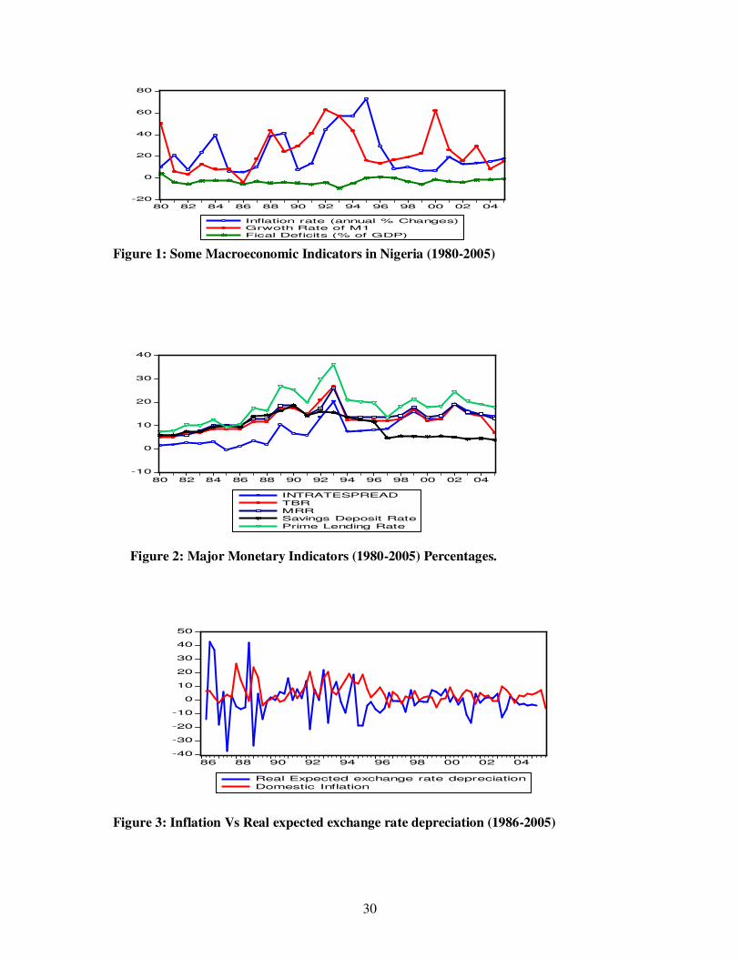
1992 before peaking at 15.5 per cent in 1993 (see Figure 1).
Insert Figure 1 here
The crowding out effect was demonstrated by changes in the direction of bank credit
flows. For instance, the share of the private sector out of a total of approximately N10.8
billion banking systems’ credit to the economy in 1980 was 67 per cent while 33 per cent
went to government. The allocation was reversed in 1992 when the shares of the government
and private sectors were in the order of 60 and 40 per cent, respectively.
The need to reverse this unsustainable trend and ensure efficient allocation of
financial resources informed the upward review of the interest rate structure. The minimum
rediscount rate (MRR) and Nigerian Treasury Bills (NTB) issue rate rose from 12.75 and
11.75 per cent in 1987-88, to 18.5 and 17.5 per cent in 1989-90, and subsequently peaked at
26.0 and 26.90 per cent, respectively, in 1993. During these periods, however, the spread
between deposits and lending rates began to widen-and became an issue of concern to the
monetary authorities. For instance, beginning from 1988, when the savings rate was about
16.4 per cent, the prime-lending rate reached 26.8 per cent, representing a spread of 10.4
percentage points, as against the stipulated limit of 7.5 percentage points. The further
widening of the spread in 1993, arising mainly from high lending rates, reflected the
oligopolistic character of the banking system. These unacceptably high lending rates were
adjudged to be a disincentive to borrowing for productive investments. Efforts to deal with
7
the situation elicited the re-introduction of measured controls on interest rates in 1993, with
the maximum lending rate pegged at 21.0 per cent (See Figure 2).
Insert Figure 2 here
The MRR was lowered during 1999 and 2000. The further lowering of the MRR,
beginning from the last quarter of 1999, was aimed at inducing a downward movement of
bank lending rates with the hope of stimulating private sector investment and economic
growth.
Moreover, the transfer of deposits of the Federal Government and its agencies from
the CBN to the commercial and merchant banks had the effect of injecting additional
liquidity into the banking system, with the expectation that it would douse the escalating
lending rates. However, experience has shown that the action, rather than ease credit for
productive investment, exerted pressures on the foreign exchange market, and enhanced
banks’ investments in NTBs thereby worsening inflationary spirals. The response of the
Central Bank of Nigeria to the pressure on the foreign exchange market was its daily
interventions in the market. The uncertainty about government next action encouraged
speculative attack on the currency, which made the intervention in the foreign exchange
market unsuccessful. Hence, expected exchange rate depreciation became an instrument for
forecasting next period inflation (Calvo, 1996; Agenor, 2004). The immediate effect of this
was further depreciation in exchange rate thereby worsening the vulnerability of the banking
system as more people switch into dollar denominated assets and deposits. Therefore, figure
3 shows the dynamics of inflation and expected exchange rate depreciation between 1986 and
2005 in Nigeria.
Insert Figure 3 here
Casual observation show that inflation and exchange rate depreciation have been
moving together over the period of our study. While causality may be difficult to establish
8
from this graph, expected exchange rate depreciation seem to be driving the inflationary
process. Agenor (2004) argued that expectation about exchange rate depreciation is a major
factor driving inflationary process in the short run. As the manufacturing sector in Nigeria is
heavily dependent on imported inputs and raw materials, every depreciation of the Naira
leads to soaring of the naira prices of such inputs and this is transmitted to the whole
economy in the form of higher prices of consumer goods and services. This consequential
increase in prices in turn resulted in increased demand for transactions money, which led to a
rise in credit and money supply. To sum up, it could be argued that accommodating monetary
policy has strengthened the inflationary impact of exchange rate depreciation.
However, since the turn of the century, the landscape has started to change. Harnessed
to a stronger political commitment, the successful consolidation in the financial sector
concluded at the end of 2005 and the unification of the foreign exchange markets in early
2006, measures such as the Fiscal Responsibility Bill, now functional monetary policy
committee (MPC), New CBN Act not permitting CBN to grant ways and means advances to
Government exceeding 5% of previous year’s revenue provided such financing is retired
before end of the financial year, are laying the foundations for improved fiscal management
of oil revenues and a better monetary policy stance. As a result, for the first time in its
history, the prospects now exist for genuinely ‘independent’ central banking in Nigeria.
Sequel to this, three important changes in monetary policy management in Nigeria are
discernible: move away from heavily managed to a more flexible exchange rates, more focus
on the price stability goal and more recognition of need for a transparent, systematic,
approach to changing the instruments of monetary policy (usually the interest rate).
3.0 Theoretical Framework
Currency substitution and monetary policy are the principal issues at hand in this
study. The motivation for them derives from the fact that the demand for money plays an
important role in the transmission mechanism of monetary policy. Indeed, empirical
estimation of money demand functions can be categorized into two: the transactions or
money services theories and portfolio theories. The transaction theories view money as a
9
medium of exchange and are demanded as an inventory for transaction purposes. Portfolio
theories consider the demand for money in much broader terms as part of the problem of
allocating wealth among a portfolio of assets, which includes money. The portfolio theories
emphasize store of value function of money. In this case, the demand for money function
becomes a portfolio optimization problem, where economic agents choose the composition of
their portfolios to maximize the returns on them. This study follows the portfolio balance
theories. As such money is viewed as a financial asset.
The demand for money as a financial asset is determined by the rate of return on the
money itself, rate of returns on alternative assets, and by the total wealth (often proxy by
income). In Friedman’s (1956) formulation, the demand for money could be expressed in real
term as.
( , , , )...............................................................................................(1)d e
iM f r y hP π=
where h is the ratio of human to non-human wealth; ir is the vector of returns on alternative
assets to money holding; Y is a measure of total wealth usually referred to as permanent
income; while eπ is the expected rate of inflation. We expect that:
0, '' >hfYf and 0, '' <ie rff π …………………………………………………(2)
More recently, Girton and Roper (1981), Cuddington (1983), Branson and Henderson
(1985) Zervoyianni (1988, 1992), Mizen and Pentecost (1996) and Rogers (1996) among
others have extended the model to include the possibility of currency substitution3. As in
Tobin (1958), these models all assume that agent maximize the returns to their wealth subject
to a given level of risk. This is the most general model since agent can hold four different
assets (namely; domestic money, foreign money, domestic bonds and foreign bonds) and
switch between them simultaneously. It is often referred to as the unrestricted portfolio
balance model of currency substitution.
Within this framework, domestic money is viewed as risk-less asset, since it is
assumed that there is no domestic inflation, while domestic bonds are risky, in that their
prices may vary. In the context of a closed economy these would be the only two assets, and
agent would choose between money and bonds on the basis of the rate of interest. Since the 3 For a nice survey of this theoretical literature, see Mizen and Pentecost (1996).
10
model is an open-economy model, there are two further assets: foreign money and foreign
bonds. The rate of return on foreign bonds is simply the rate of interest plus the expected
depreciation of the domestic currency, since for domestic residents it is the home-currency
value of bond returns that is important. The rate of return on foreign money, in the absence of
inflation, is again zero.
In practice, however, inflation is rarely zero. In the case of non-zero inflation, in both
the home and the foreign country the return on cash holding is the inverse of the inflation
rate. Therefore, the relative return on the cash part of the portfolio is given by the expected
depreciation of the exchange rate. Thus if domestic inflation is expected to be higher than
foreign inflation, the domestic currency is expected to depreciate and the demand for
domestic currency will fall relative to foreign currency.
Branson and Henderson (1985) assume that the domestic demand (i.e. that of
domestic residents) for assets depends on their relative returns, satisfying the usual wealth
constraints:
*{ , , , , , }e eM m i i e y Wπ− − +− + +
= …………………………………………………… (3)
* * *{ , , , , , }e eeM M i i e y Wπ− + +− + +
= ………………………………………………... (4)
*{ , , , , , }e eB B i i e y Wπ− − −+ − +
= …………………………………………………….. (5)
* *{ , , , , , }e eeB B i i e y Wπ+ − −− − +
= …………………………………………………… (6)
The first argument in equations (3)-(6), i , is the return on holding bonds denominated
in domestic currency relative to the return on domestic money (minus the rate of domestic
inflation). It is assumed that all four assets are substitutes in the portfolio. Hence, an
increase in i raises the demand for domestic bonds but lowers the demand for their
substitutes in the portfolio. The nominal return on bonds denominated in foreign currency is
*i . This return expressed in terms of domestic currency becomes *( )ei e+ , where ee is the
expected change in the exchange rate. It affects the demand for foreign securities positively
and that for other assets negatively. Once again, this second argument is in fact a real return
11
differential, where the return on domestic money is minus the rate of inflation. Similarly, the
third argument, ee , is the expected change in the exchange rate.
The fourth argument, y , is the home currency value of domestic output and affects
demand for all assets positively. eπ is a measure of domestic inflation. An increase in eπ
increases the demand for both moneys and lowers the demand for bonds denominated in
domestic and foreign currency. The positive effect of domestic wealth W, the last argument,
reflects the assumption that all assets are “normal assets”.
The advantage of the portfolio balance approach is that it distinguishes between
currency substitution, as measured by the coefficient on the expected change in the exchange
rate, and capital mobility, as measured by the coefficient on the foreign rate of interest.
Another interesting feature of these types of models is that it can be estimated for individual
domestic-money demands, as in Cuddington (1983) or Mizen and Pentecost (1994) or as an
aggregate demand for money over a specific region. For our purpose, we estimate this
equation for the Nigerian economy using quarterly data for 1986q1 to 2005q2.
4.0 Model Specification
In an empirical context, it is most common to estimate just the demand for money
function of the form specified in equation (3) (Miles, 1978 and Cuddington, 1983). We
estimate a variant of equation (3) by replacing domestic money demand with currency
substitution index, which is the focus of this study. From equation (3), we assume rational
expectations when expectations are formed about exchange rates.
To sketch the analysis, let tX denote a vector of endogenous variables. Specifically,
the model specification is of the form:
* /( , , , , , , ) .......................................................................(7)et t t t t t t tX i CSI e ERV y iπ=
where all variables except interest rates are expressed in logarithms. ete , the expected change
in the exchange rate, ti the domestic policy interest rate, tCSI is currency substitution index,
ty is the home-currency value of domestic output, measured by GDP, tπ is domestic inflation,
*ti denotes foreign rate of interest, proxy by Federal Funds rate plus expected exchange rate
12
changes (i.e. * ei ffr e= + ), where ffr is US federal funds rate and tERV is a measure of
exchange rate volatility.
Following Kim and Roubini (1999) and Clarida and Gertler (1997), we choose to
consider the real rather than the nominal exchange rate. According to sticky price models, the
two rates have an identical pattern in the short run, so that the real exchange rate inherits the
asset price nature of the nominal one. Moreover, the real exchange rate plays a more
important role in the transmission mechanism of monetary policy and, therefore, is more
informative to study the dynamics of the non-policy variables.
A measure of exchange rate volatility, tERV , is included to capture both the absolute
domestic-money-demand depressing effects of volatility and any substitution away from
domestic assets demand to foreign assets demands due to a rise in volatility. We expect
exchange rate volatility to increase the desire of domestic residents to want to switch to
demanding for foreign currencies and deposits. Following Ndung’u (2001), the conditional
volatility of exchange rate was extracted and modeled via a state space representation of the
form: -
12
21
; __________ (0,1)................................................(8)
__________ (0, ) 1....................................(9)
tht t t
t t t
Z e iid
where
h h NID µ
σε ε
λ µ σ λ+
=
= + ≤
tZ is the parallel market exchange rate. The term σ2 is a scale factor and subsumes the effect
of a constant in the regression of ht, λ , is a parameter, tµ is a disturbance term that is
uncorrelated with tε , tε is an (0,1)iid with random disturbances symmetrically distributed
about zero. The ht equation is a transition equation in autoregressive form where the absolute
value of λ is less than unity to ensure that the process in equation (9) is stationary (Ndung’u,
2001). These equations generate the conditional volatility of exchange rate used in the Vector
Error Correction Models (VECM).
The foreign rate of interest, *ti , proxy by the Federal Funds rate, is included to control
for the response of domestic economy to US financial variables and how foreign rates of
returns affect the portfolio of assets of domestic residents especially currency substitution.
13
Therefore, *ti is included to account for how it encourages or discourages currency
substitution in Nigeria as people switch from the demand from domestic money to foreign
money. Kim and Roubini (1999) cite evidence in Grilli and Roubini (1996) that this is
important for G6 countries. For our purpose, Nigeria has had relatively open capital markets,
especially as from 1986 when financial liberalization started, and it is also reasonable to
assume that domestic interest rates are related to US interest rates. This means that the US is
serving as a proxy for the international economy. Indeed, there is sufficient evidence to
suggest that the US has an important influence on Nigerian financial variables and is likely to
act as a reasonable proxy (see Dungey and Pagan, 1998, for similar explanations).
The interest rate equation is interpreted as the policy reaction function of the central
bank. The interest rate used is the treasury bills rate. This interest rate has been the principal
policy instrument of the Central Bank of Nigeria as from 1986 when liberalization started.
For our purpose, the policy reaction function of the central bank depends contemporaneously
on all the variables in the model. This is a departure from Brischetto and Voss (1999)
specification for Australia, which included only three variables (oil price used as a proxy for
anticipated inflation; domestic monetary aggregate and nominal exchange rate) in the interest
rate equation. Indeed, excluding output from the interest equation amounts to restricting the
monetary authorities from responding to any indicators of future output apart from those
specified in the model. For our purpose, we consider this inappropriate given the structure of
Nigerian economy. Indeed, by including output, price level and all other variables in the
interest rate policy equation, we are able to account for how unanticipated monetary policy
shocks affect those variables in the system. Also, we follow Cushman and Zha (1997) model
for Canada, which includes the US Federal Funds rate in the domestic policy reaction
function. They argued that inclusion of this variable is important in their model in order to
account for the effects of foreign variables on the domestic economy. Hence, we include the
contemporaneous US Federal Funds rate in the domestic interest rate equation in order to
obtain sensible dynamic responses. Also, currency substitution index was included in the
model to account for the effect of using foreign currency (as store of value), in the domestic
economy, on the conduct of monetary policy in Nigeria.
14
Finally, the model was restructured such that we used exchange rate as a measure of
monetary policy. In this case, the exchange rate is treated as dependent upon all innovations
of the model. This reflects the fact that the exchange rate is a financial variable and reacts
quickly to all information. Aside from this, the exchange rate is an indirect tool of monetary
policy especially in a free market economy where exchange rates are allowed to float. A
similar argument was employed by Cushman and Zha (1997) and also, by Brischetto and
Voss (1999). This allows us to compare the use of interest rate or exchange rate for
stabilization purposes within the domestic economy in the face of currency substitution.
The empirical exercise is to model and estimate the dynamic interactions among the
variables in a VECM. We proceed with the endogenous variables n=7, and assume that the
structure of the model is consistent with the class of dynamic linear stochastic models, which
can be represented as:
( ) ........................................................................(10)t tD L X µ∆ =
where L is the shift operator, tµ is a vector of white noise errors and Di are (7x7) matrixes of
finite coefficients that summarize the dynamics of the model. Each of the jtµ is to be
interpreted as an exogenous structural shock to the jth equation. For example, j = 4 represents
the exchange rate volatility equation and thus t4µ is a random variable depicting the
innovation to the exchange rate volatility process.
The sample second moments of the joint probability distribution generating the data
are fully summarized by the following Wold moving average representation:
( ) ( )( ) ( )22 ...t I t tX I D L D L D Lµ µ= + + + = (11)
where ( ) �=1µµtE
If the data generating process for tX is covariance stationary, then 0lim =→∝ ss D .
Furthermore, if ( )D L is invertible, then the coefficient in ( )D L and � are directly
obtainable from the following VAR representation of tX :
( ) ( ) 1t t tA L X C L X v−= = (12)
15
where ( )A L is a thk matrix of polynomials in the lag operator L with all roots inside the unit
circle and tv is a vector of zero-mean, independently and identically distributed innovations
with a covariance matrix� .
But one problem that arises is that Equation (10) is consistent with any linear
theoretical model and thus had little empirical content. We thus require further restrictions so
that ( )D L can be uniquely identified. In the VAR literature, the choice of identifying
restrictions is based on a priori economic reasoning regarding the structure of the system. The
most commonly used restriction is the recursive system (triangularization) where the
innovations of the first variable in the system affect all variables and the innovations of the
last variable contemporaneously affect only that variable.
This method has basic weaknesses by imposing a recursive structure in the dynamic
analysis and may not be adequate for evaluating the effects of structural economic
disturbances as this study intends to do. The method has been convenient and easy to apply
but is inconsistent with any plausible model. To resolve these empirical weaknesses and
identify the desired dynamic multipliers we use restrictions from the economic model itself.
The most important aspect of this analysis is to analyse the causal structure of the variables in
the system. The causal structure will show which variables affect all the other variables and
thus determine their position in the matrix (Ndung’u, 2001).
The next task is to identify monetary policy in the model. Two approaches to solving
identification problem include: imposing short run or long run restrictions. However, Faust
and Leeper (1997) criticized long run restriction on the ground that ��������������������� �
��� ����� � ��� ������� �������� �� � ��� ���� ����� ������� �� ����� ���� �� ���� ������� ��
� ������� ������������������������������������� �� ����� !!"#$������� ����������
�����������������%�� ������ ����&������%����������� ����$� ���� � ��������������������� ���
����� ����� ���������� ��� ���� � ��� � ��� ����� � ������������%� �� ������%�
���%��&������������������������������'����������������������������������������������
����� �������������������%����%��Also, innovations in foreign rate of interest *ti , are
due to “own” shocks. By implication, this restriction shows that innovations in foreign rate of
interest do not depend on innovations from other variables in the model since domestic
16
financial factors cannot influence the US rates of interest. Hence, the ordering implied by this
identification is as shown in equation (7).
5.0 Data, Econometric Procedure and Results
All variables4 are measured at log levels except for the interest rates, which are in
percentages, i.e. all variables appear as rates of change rather than in levels. Because
inferences drawn from VAR models and its variants may be sensitive to specification (levels
or first differences and inclusion or exclusion of time trend), the time series properties of the
data were carefully evaluated5. The Augmented Dickey Fuller (ADF) and Philip-Peron (PP)
tests suggest that our variables are (1)I . The Johansen (1988) cointegration test suggests that
the variables are cointegrated6 meaning that long run stable relationship exists among the
variables.
The theoretical exposition of VAR methodology is based on the implicit assumption
that the lag order is known (Hamilton, 1994). In empirical applications however, the optimal
lag order is typically unknown and hence it must be determined. Based on several criteria7
(AIC, FPE, and LR tests), a lag order of 4, which produced a stable VECM, was selected.
The net task is whether to estimate a VAR in first difference or a VECM in levels.
With cointegration between two or more of (1)I variables, VAR models in first difference
are misspecified (Hamilton, 1994) and a VECM should be applied to the level of the
cointegrated series. Hamilton (1994) asserts, “…if [a set of variable] are cointegrated, then it
is not correct to fit a vector autoregression to the differenced data. The correct empirical
procedure is to estimate a VECM on the variables at levels.” This suggests the existence of a
long run relationship among the variables (Johansen, 1988). Thus, we estimated a VECM.
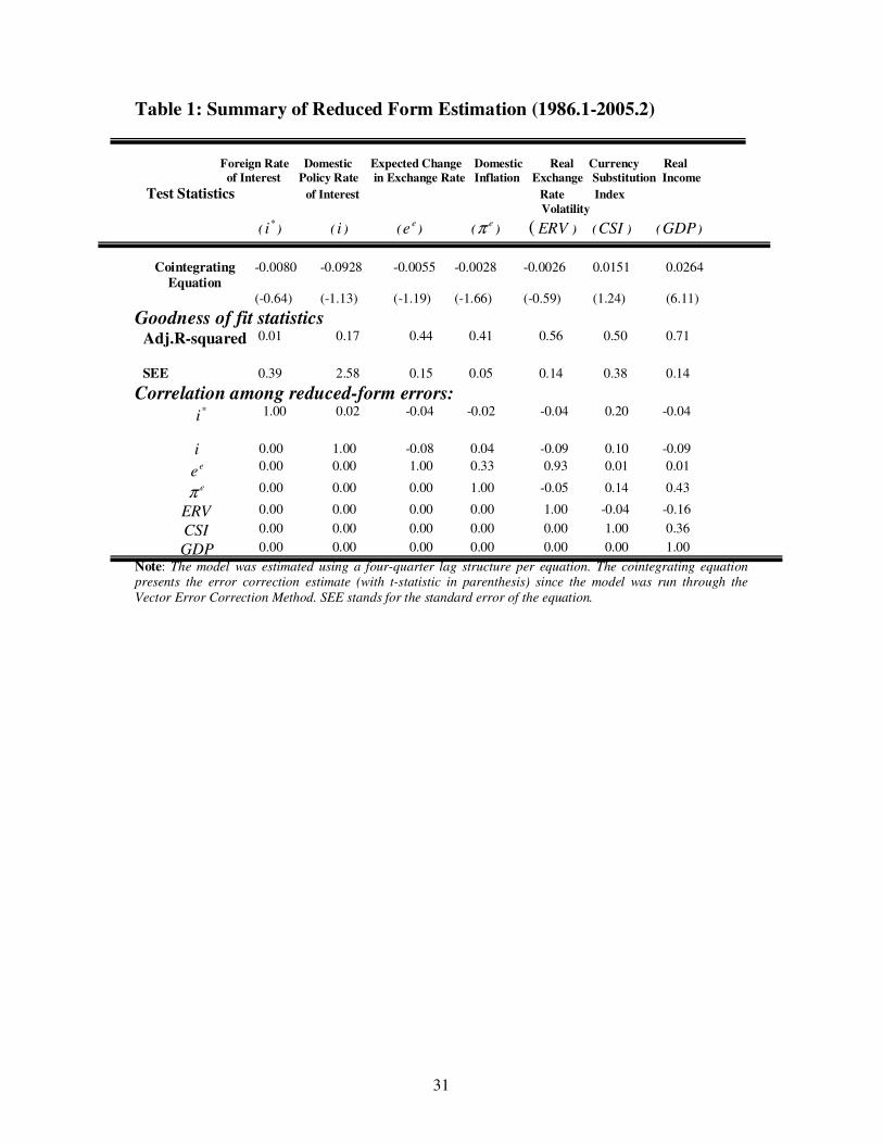
5.1 Reduced-Form Estimation Results
The fact that the variables are cointegrated justifies the use of VECM. The VECM
allows the long-term behaviour of the endogenous variables to converge to long-term
equilibrium relationships while allowing a wide range of short-term dynamics. The
cointegration relationships are presented in the first panel of Table 1. Evidence from Table 1 4 Appendix 1 contains explicit data definition, measurements and sources. 5 To conserve space, the Unit roots test results are not presented here but is available on request. 6 For similar reasons, the cointegration table is not reported here. 7 See Lutkepohl, (1993) for a review of popular selection criteria
17
suggests that domestic income, domestic policy rate of interest, expected change in exchange
rate, inflation and currency substitution adjusts to the deviations from their long-term paths
within four quarter, unlike foreign rate of interest and real exchange rate volatility.
However, this long-term relationship is significant at 1 percent for domestic income
(GDP), and 10 percent for domestic policy rate of interest, expected change in exchange rate,
inflation and a measure of currency substitution. Foreign rate of interest and real exchange
rate volatility tend to show that there is absence of convergence to equilibrium paths. In all,
the result in Table 1 indicates that the adjustment process takes longer time for foreign rate of
interest, real exchange rate volatility, monetary policy, domestic inflation, currency
substitution measure and indeed expected change in exchange rate. As presented in the
second panel of Table 1, the model explains a significant proportion of the variability of the
series, principally for domestic income and real exchange rate volatility, followed by the
currency substitution, expected change in exchange rate, domestic inflation, and domestic
policy rate of interest and least for the foreign rate of interest. The very low value of 2R for
foreign rate of interest model reflects the fact that identified domestic macroeconomic factors
in Nigeria explains only about 1 percent of the variations in the foreign rate of interest.
Altogether, the standard errors of the equations are plausibly low except for domestic policy
rate of interest equation, which is slightly high.
Insert Table 1 here
The summary of the correlation matrix is as presented in the last panel of Table 1.
The result indicates that there is a high and positive correlation between real exchange rate
volatility and expectations about exchange rate changes in Nigeria. Also, the correlation
between expected exchange rate changes and domestic inflation is very interesting although
expected. It shows that market agents’ expectation about exchange rate depreciation
encourages domestic inflation in Nigeria. This is particularly relevant for Nigeria since the
introduction of structural adjustment programme when market forces determine all rates. A
significant development in Nigeria following this policy shift has been speculative businesses
in the foreign exchange market. This had more often than not encouraged exchange rate
18
volatility with its pass-through effects to domestic inflation. Again, the correlation between
expected change in exchange rate and domestic policy rate of interest indicates that market
agents expectation about macroeconomic fundamentals especially exchange rate changes in
Nigeria is always at conflict with monetary policy stance of the government. This is reflected
by the negative value of the correlation between the two variables. Also, note that currency
substitution is relatively more correlated with foreign rate of interest, domestic inflation and
monetary policy stance or credibility in Nigeria (see Table 1). This is in line with the findings
of most empirical literature on currency substitution (see, Gruben and McLeod, 2004 and
Agenor, 2004).
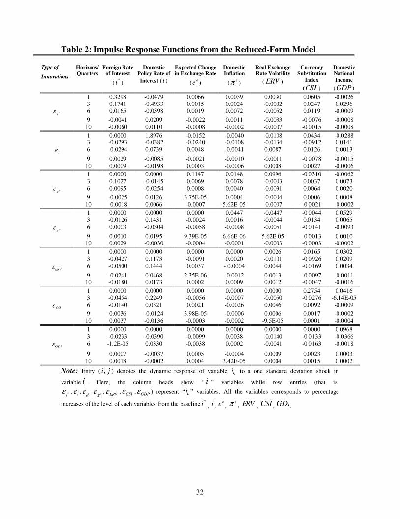
5.2 Impulse Response Functions
Since the focus of this section is to determine how currency substitution and exchange
rate volatility responds to monetary policy in Nigeria, we therefore constructed the impulse
response functions from the VECM to trace the response of one variable to a one standard
deviation shock to monetary policy and this can be thought of as a type of dynamic multiplier
(Prock, Soydemir and Abugri, 2003). Table 2 depicts the impulse response functions of the
variables described above, using a horizon of ten quarters. Table 2 shows the responses of a
particular variable to a one-time shock in each of the variables in the system. This allows us
to address directly issues concerning the implications of exchange rate volatility and currency
substitution for monetary policy in Nigeria.
In this case, we consider the response of currency substitution and exchange rate
volatility to monetary policy in Nigeria i.e. the first issue addressed has to do with how does
exchange rate volatility and currency substitution responds to monetary policy in Nigeria.
This will allow us to determine the potency of monetary policy in containing or managing
exchange rate volatility and currency substitution episodes in Nigeria. However, we consider
two possibilities: when interest rate is used as a policy instrument and when exchange rate is
used as a policy instrument.8
5.2.1 Impulse Responses: The Interest rate as a Policy Instrument
8 It has been argued that under a flexible exchange rate system, exchange rate is an indirect tool of monetary policy (see for example, Fung, 2002). Therefore, in what follows, we examine each of these issues more closely.
19
Table 2 shows the impulse response functions of the variables included in the VECM
to a monetary policy shock that results in a one-standard deviation rise in the domestic rate of
interest. Following a contractionary monetary policy shock, it is expected that output, prices
and currency substitution will all fall while the exchange rate will appreciate. It can be
observed that following a contractionary monetary policy shock; output fell immediately but
oscillates between the sixth and ninth quarters before fading away towards the tenth quarter.
As expected, a tightening shock leads to a persistent fall in domestic prices both in the short
term and in the longer horizon. Although, this behaviour of the data is supported by economic
theory, but our knowledge of economic history of Nigeria reveals that more often that not
prices in Nigeria do not always fall persistently as a response to any monetary policy
initiative of the government. In most cases, when prices go up, they never come down.
Although a rise in domestic interest rate leads to an increase in currency substitution in the
first quarter, the effect is not significant and oscillates thereafter. This point to the fact that
currency substitution is not an instant reaction to the slightest policy mistake since it takes
time before people switch into holding foreign currency. But once they do, bringing about a
reversal may be difficult. This finding is consistent with the observation of Dornbusch and
Reynoso (1993) in a study of the Latin American countries. It was argued that when
economic and political instability is pervasive, the response of market agents would be a shift
into foreign currency assets in the form of currency or real and financial assets located abroad
even when domestic rate of interest is high.
Next we look at the effect of monetary policy shocks on exchange rate volatility in
Nigeria. The impulse response function presented in Table 2 shows that a one-time standard
deviation shock to monetary policy variable will dampen (reduce) exchange rate volatility in
the first and third quarters while it fuels volatility around the sixth quarter and oscillates
thereafter. The conclusion that can be drawn from this is that monetary policy can be used to
dampen real exchange rate volatility only in the short and medium horizon but may not be
effective in the longer horizon. These results are generally in line with most empirical studies
in this area (see, Dungey and Pagan, 1998 and Prock, Soydemir and Abugri, 2003). Similarly,
we find that the effect of monetary policy on the level of output is largest in the first and third
20
quarters out which follow a hump shape as reported by Bernanke and Mihov (1998), Walsh,
(2003) for the American economy.
5.2.2 Impulse Responses: The Exchange rate as the Policy Instrument
Following financial sector reforms and the subsequent liberalization of capital account
in Nigeria, the instability in the exchange rate has made it mandatory for policy makers to
initiate policy aimed at reducing this swing in exchange rate. The approach followed in
Nigeria has been periodic intervention (daily or weekly depending on the level of expected
instability) in the foreign exchange market largely by selling or buying foreign exchange in
the market thereby using exchange rate as a policy instrument. The idea is that since, market
agents do not have perfect information about the timing and magnitude of intervention, then,
such actions becomes exogenous. Therefore, such action could be perceived as an exogenous
policy action. In this section, the results of the impulse response function in the case where
the effective exchange rate is used as the monetary policy instrument are reported. Precisely,
we look at the responses of all the variables included in the VECM to a monetary policy
shock that results in a one-standard deviation change in the exchange rate following policy
intervention.
Following a monetary policy shock that results in an appreciation of the effective
exchange rate through central bank intervention in the foreign exchange market, output,
prices, money, the interest rate and exchange rate volatility are expected to fall. The results
presented in Table 2 indicate that depreciation in the Naira exchange rate following financial
liberalization resulted in a persistent increase in domestic inflation in Nigeria. The impact
however fades away towards the 9th quarter. The response of real exchange rate volatility to a
one standard deviation shock to exchange rate in Nigeria is mixed. In the first place,
depreciation in the Naira/ US dollar exchange rate resulted in increased volatility especially
from the third quarter onwards. However, this affects die out towards the ninth quarter. This
point to the fact that exchange rate liberalization in Nigeria created increased uncertainties in
the system that aggravated the erratic behaviour of exchange rate in Nigeria. The erratic
behaviour of the exchange rate made planning difficult and therefore encouraged speculative
activities, which more often than not encourages exchange rate volatility in Nigeria.
21
Next we consider the effects of monetary policy shocks using exchange rate as a
policy variable on currency substitution in Nigeria. The impulse response function presented
in Table 2 shows that a one-standard deviation shock to monetary policy variable will
dampen currency substitution in the first and tenth quarter while it encourages currency
substitution in the third, sixth and the ninth quarter. This point to the fact that exchange rate
depreciation reduces the value of peoples’ assets denominated in domestic currency and as
such encourages currency substitution in favour of more stable currency like the U.S. dollar.
Finally, we look at the response of output (GDP) to a one-time standard deviation
shocks to monetary policy variable in Nigeria. The result from the impulse
response function indicate that exchange rate appreciation leads to a fall in domestic output
(as indicated by the figure in the first and tenth quarters), while a depreciation will result in
an increase in domestic output (as indicated by values in the third, sixth, and ninth quarters of
column nine of Table 2).
Overall, modeling the effective exchange rate as the monetary policy instrument
produces results that are consistent with the conventional thinking about the monetary
transmission mechanism. This result is quite interesting because, unlike in the case using the
interest rate as the instrument, there are other factors affecting the exchange rate that may not
be captured by the variables included in the VECM. For example, capital flows due to foreign
direct investment in Nigeria could move the exchange rate but are unlikely to be accounted
for by the macroeconomic variables included. However, this exogenous exchange rate
movement may be interpreted as a monetary policy shock in the VECM. This is in line with
the finding of Fung, (2002) study for the East Asian economies. Nevertheless, the result
suggests that the VECM model is capable of identifying the exogenous monetary policy
shock that results in an appreciation of the nominal effective exchange rate.
Insert Table 2 here
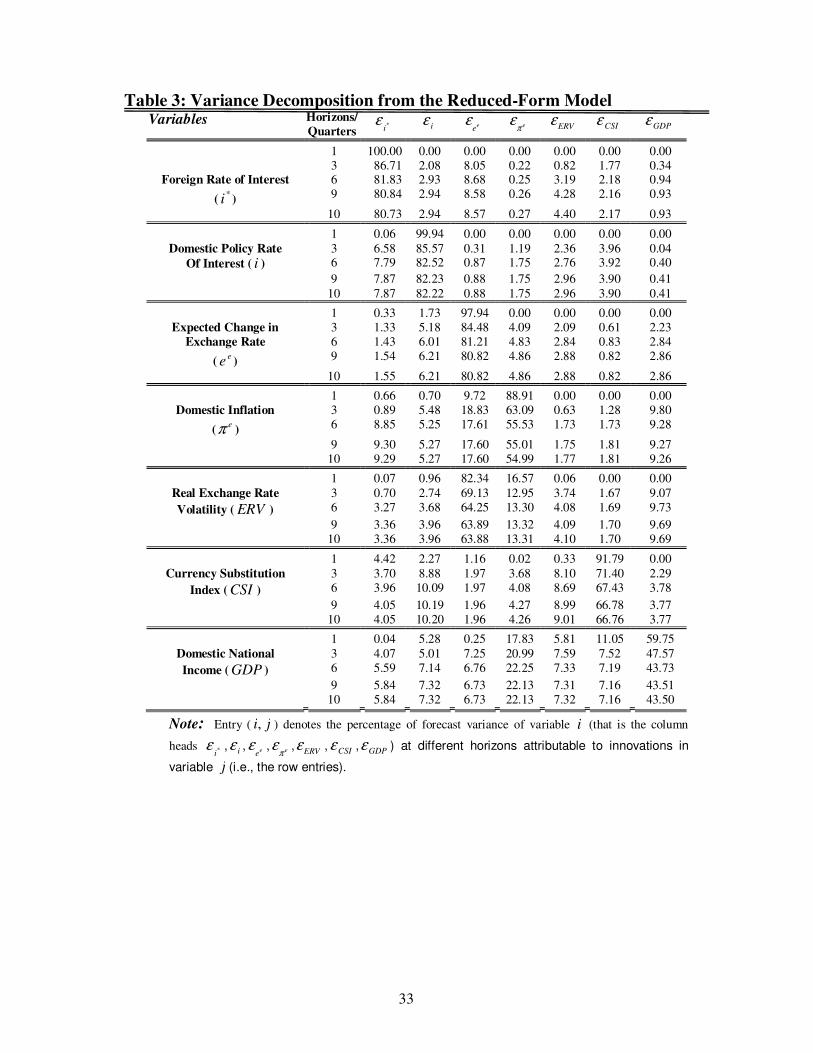
5.3 Forecast Error Variance Decomposition Results
22
In addition to the impulse response function results presented above, we also obtained
the variance decomposition. While impulse response functions trace the effects of a shock to
one endogenous variable on to the other variables in the VECM, variance decomposition
separates the variation in an endogenous variable into the component shocks to the VECM.
Thus the variance decomposition provides information about the relative importance of each
random innovation in affecting the variables in the VECM. In Table 3, we report the
proportion of the forecast error variance of each variable accounted for by the innovations to
each of the structural equations. Results are reported for forecast horizons 1, 3, 6, 9 and 10
quarters ahead. They show the fraction of the forecast error variance for each variable that is
attributable to its own shocks and to shocks in the other variables in the system.
Mirroring results from previous studies in the VECM literature, the predominant
sources of variation in all the variables in the system are the “own” shocks. Foreign rate of
interest is an important source of the forecast errors in the domestic policy rate of interest
followed by currency substitution, real exchange rate volatility and domestic inflation in that
other. Foreign rate of interest accounts for less than 1 percent in the first two quarters away
but account for more than 7 percent forecast error variance in the longer horizons. This can
be interpreted to mean that foreign rate of interest and indeed U.S monetary policy has a
significant effect on Nigeria’s monetary policy especially in the longer horizons. Another
very interesting discovery has to do with the contribution of currency substitution to forecast
error variance in domestic policy rate of interest in Nigeria. This may be interpreted to mean
that formulating domestic monetary policy without taking into consideration this important
variable may lead to ineffectiveness of monetary policy in Nigeria. This supports both
theoretical and empirical literatures on currency substitution. See for example, Seater (2002)
for theoretical discussions and Friedman and Verbetsky (2001) for the Russian economy.
Also, real exchange rate volatility account for about 3 percent of the forecast error variance of
monetary policy. This means that exchange rate volatility may frustrate monetary policy
intentions due to it destabilizing effects by introducing uncertainty into the system thereby
making planning difficult.
Innovations in domestic monetary policy account for about 6 percent, 5 percent, 4
percent, 10 percent and 7 percent of the forecast error variance in expected exchange rate
23
changes, domestic inflation, real exchange rate volatility, currency substitution and domestic
national income respectively. Another striking discovery is the role of currency substitution
in explaining forecast error variance in domestic income. Currency substitution account for
about 11percent of the forecast variance error in the short run although the contribution
decline to about 7 percent in the longer horizon. This may mean that the existence of
currency substitution indicates income loss to a dollarised economy. This supports the views
of D’Arista (2000) about income loss due to currency substitution.
In a similar vein, domestic policy rate of interest and real exchange rate volatility
account for a larger proportion of the forecast error variance in currency substitution in
Nigeria than other variables included in the model aside from own shocks. Specifically, it
could be seen from Table 3 that innovations to monetary policy alone account for about 10
percent of the forecast error variance in currency substitution while real exchange rate
volatility account for about 9 percent especially in the longer horizon. This could be
interpreted to mean that monetary policy may be a weak weapon in reversing currency
substitution in Nigeria going by the level of the variance error explained by monetary policy.
Again, price is an important source of forecast error variance in gross domestic output
explaining about 22 percent of the forecast error variance in GDP while currency substitution,
domestic policy rate of interest and real exchange rate volatility each account for about 7
percent of the forecast error variance in domestic income (GDP) particularly in the medium
and long term horizons. The contributions of innovations to domestic monetary policy are of
interest and we find results that are generally in support of the findings in the literature.
Innovations to monetary policy contribute very little to forecast error variance of output,
contributing only approximately 5 percent in the medium horizons and about 7 percent in the
longer horizons. This is similar in magnitude to results reported in Dungey and Pagan (1998),
and Brischetto and Voss (1999) in their empirical model of monetary policy in Australia. Our
results are also broadly consistent with the general findings from the structural VAR
literature- innovations to domestic monetary policy have very little effect on output.
Contrary to the findings of Brischetto and Voss (1999) reported for the Australian
economy and most U.S literature on monetary policy, to the effect that monetary policy
innovations contribute very little to the forecast error variance of monetary policy instrument
24
itself i.e. interest rate, we finds that for the Nigerian economy, this proposition do not hold.
As presented in Table 3, we note that innovations to monetary policy account for over 99
percent of the forecast error variance in self in the medium horizons and over 82 percent in
the longer horizons.
Finally, innovations to market agents’ expectation about future changes in exchange
rate accounts for about 18 percent of the forecast error variance in domestic inflation in the
medium term while it accounts for about 17 percent in the longer horizons. This explains the
pass-through effects of expected exchange rate depreciation to domestic prices in Nigeria.
Insert Table 3 here
5.4 Conclusion In this study, empirical evidence on the response of exchange rate volatility and
currency substitution to monetary policy shocks in Nigeria in a multivariate setting was
analyzed. Both the impulse response and the forecast error variance decomposition were
constructed. Our results from both functions suggest the following conclusions: One,
exchange rate volatility respond to monetary policy with some lags. For example, monetary
policy will not affect exchange rate volatility until three quarters away. Two, a tightening
shock leads to a persistent fall in domestic prices both in the short term and in the longer
horizon. Currency substitution is not an instant reaction to the slightest policy mistake rather;
it is fallout from prolonged period of mismanagement and macroeconomic instability. Indeed,
it takes time before people will switch into holding foreign currency. But once they do,
reversal may be difficult.
In terms of policy choice, it could be concluded that exchange rate-based monetary
policy would be more potent in reducing currency substitution than interest rate-based policy.
Specifically, exchange rate volatility must be brought under control by pursuing deflationary
policy. However, the effect on output loss of deflationary policy must also be compared to
the gains of reducing currency substitution at the margin.
Our results from the forecast error variance decomposition reveal that the predominant
sources of variation in all the variables in the system are the “own” shocks. Foreign rate of
interest is an important source of the forecast errors in the domestic policy rate of interest
followed by currency substitution, real exchange rate volatility and domestic inflation in that
other. Finally, innovations to market agents’ expectation about future changes in exchange

25
rate accounts for about 18 percent of the forecast error variance in domestic inflation in the
medium term while it accounts for about 17 percent in the longer horizons. This explains the
pass-through effects of expected exchange rate depreciation to domestic prices in Nigeria.
26
References Adams, C. and B. Goderis, 2006. Monetary policy and oil price surges in Nigeria, A paper
prepared for the Central Bank of Nigeria Workshop on Economic Policy Options for a Prosperous Nigeria, Abuja, October 23-24.
Agenor, P. 2004. The Economics of Adjustment and Growth, Second Edition, Harvard University Press, Cambridge Massachusetts.
Akinlo, A. E. 2003. Exchange Rate Depreciation and Currency Substitution in Nigeria. African Review of Money, Finance and Banking, Supplementary Issue of “Savings and Development” 2003. Italy.
Bernanke, Ben, and Ilian Mihov, 1998. Measuring Monetary Policy. The Quarterly Journal of Economics, Vol. 113(3):869-902.
Branson, W.H. and D.W. Henderson, 1985. The Specification and Influence of Asset Markets’, in R.W. Jones and P.B. Kenen (eds). Handbook of International Economics. Vol. II. Amsrerdam: North Holland.
Brischetto, Andrea and Graham Voss, 1999. A Structural Vector Autoregression Model of Monetary Policy in Australia, Research Discussion paper 1999-11, Economic Research Department, Reserve Bank of Australia, pp. 1-55.
Calvo, G.A. 1996. Money, Exchange Rates and Output. The MIT Press, Cambridge Massachusetts.
Central Bank of Nigeria, 2007. Direction of Monetary Policy Beyond 2007, Clarida, Richard, and Mark Gertler, 1997. How the Bundesbank Conducts Monetary Policy.
in Christina Romer and David Romer, eds., Reducing Inflation: Motivation and Strategy, University of Chicago Press for NBER.
Corrado, G. 2008. An open economy model with currency substitution and real dollarization, Journal of Economic Studies, Vol. 35(1):69-93.
Cuddington, J.T. 1983. Currency Substitutability, Capital Mobility and Money Demand. Journal of International Money and Finance, Vol. 2:111-33.
Cushman, D.O. and T.A. Zha, 1997. Identifying Monetary Policy in a Small Open Economy Under Flexible Exchange Rates. Journal of Monetary Economics, Vol. 39(3):433-448.
D’Arista, Jane, 2000. Dollarization: Critical U.S views. Paper presented at a conference On: To dollarize or not to dollarize: exchange-rate choices for the western hemisphere, (Oct. 4-5) Ottawa, Canada.
Dornbusch, R. and A. Reynoso, 1993. Financial Factors in Economic Development. In R. Dornbusch (ed.), Policy Making in the Open Economy: Concepts and Case Studies in Economic Performance, Oxford University Press.
Dungey, M. and A. Pagan, 1998. Towards a structural VAR for the Australian Economy. Latrobe University, Mimeo.
Faust, Jon and Eric M. Leeper. 1997. When Do Long-Run Identifying Restrictions Give Reliable Results? Journal of Business and Economic Statistics. Vol. 15(3):345 – 354.
Friedman, A.A. and A. D. Verbetsky, 2001. Currency Substitution in Russia. Economics Education and Research Consortium Working Paper Series, Working Paper No 01/05
Friedman, M. 1956. The Quantity Theory of Money: A restatement. in M. Friedman, editor, Studies in the Quantity Theory of Money. Chicago: University of Chicago Press. Reprinted in Friedman, 1969
Fung, Ben S.C. 2002. A VAR Analysis of the Effects of Monetary Policy in East Asia. BIS Working Papers No. 119, Bank For International Settlements, Monetary and Economic Department.
27
Girton, L. and D. Roper, 1981. Theory and implication of currency substitution. Journal of Money, Credit and Banking, Vol.13(1):12-30.
Grilli, V. and N. Roubini, 1996. Liquidity Models in Open Economies. European Economic Review, Vol. 40:847-859.
Gruben, W.C and Darryl McLeod, 2004. Currency Competition and Inflation Convergence. Center for Latin American Economics, Federal Reserve Bank of Dallas. http://www.fordham.edu/economics/mcleod, accessed April, 2006. ������� � � ��� ��� ����������� �
Time Series Analysis����� � ���� � � ������� ��� � ������ ����� ����� ��� � !��� ��� ���
" #�$�� %�����&�� " ��������'�� ()� ������� ����&������ ��+*���, �� �-�!���%�.!� �/�� $0�,�1�� 2�� � � � 3���� #������ ���� 4 ��� � � �" ��5���6�� *�� ()��&���� � ����� �����7�����8 ()��9�� : �
Ikhide S.I 1996. Financial sector Reform and Monetary Policy in Nigeria. IDS Working Paper, 68
Johansen, S. 1988. Statistical Analysis of Cointegration Vectors. Journal of Economic Dynamics and Control, Vol. 12:231-54 (June-September).
Kim, S. and N. Roubini, 1999. Exchange Rate Anomalies in the Industrial Countries: A solution with a Structural VAR Approach. University of Illinois, Urbana-Champaign, Mineo.
Lutkepohl, H. 1993. Introduction to Multiple Time Series Analysis, Springer, Berlin. Miles. M.A. 1978. Currency substitution, flexible exchange rates and monetary
independence. American Economic Review, Vol. 68:428-36. Mizen, P.D. and E.J. Pentecost, 1996. Currency Substitution in Theory and Practice. in
Mizen, P. and J. Pentecost (eds.) The Macroeconomics of International Currencies: Theory, Policy and Evidence. Edward Elgar Publishing Company. USA
Mizen, P.D. and E.J. Pentecost, 1994. Evaluating the Empirical Evidence for Currency Substitution: A Case Study of the Demand for Sterling in Europe. The Economic Journal, Vol. 104:1057-69.
Ndekwu, E.C. 1995. Monetary Policy and the Liberalization of the Financial Sector. in Akin Iwayemi (ed.) Macroeconomic Policy Issues in an Open Development, NCEMA. Ibadan.
Ndung’u, N.S. 2001. Liberalization of the foreign exchange market and the short-term capital flows problem, AERC Research Papers 109, African Economic Research Consortium, Nairobi, Kenya.
Ojo, M.O. 1992. Monetary Policy in Nigeria in the 1980s and prospects in the 1990s. CBN, Economic and Financial Review, Vol. 30(1):
Olomola, P.A. 1999. An Empirical Investigation of Currency Substitution in Nigeria. Ife Journal of Economics and Finance, Vol. 4(1 & 2):
Oresotu, F.O. and N.O. Mordi 1992. The Demand for Money Function in Nigeria: An Empirical Investigation. Central Bank of Nigeria, Economic and Financial Review, Vol. 30(1):32-69
Prock, Jerry, Gokce A. Soydemir and Benjamin A. Abugri, 2003. Cuurency Substitution: Evidence from Latin America. Journal of policy Modeling, Vol. 25:415-430.
Reinhart, C., K. Rogoff and M. Savastano (2003). ‘Addicted to dollars’, NBER Working Paper No. 10015.
Rogers, J.H. 1996. The Currency Substitution Hypothesis And Relative Money Demand In Mexico And Canada. in Mizen, P. and J. Pentecost (eds.) The Macroeconomics of International Currencies: Theory, Policy and Evidence. Edward Elgar Publishing Company. USA.
Sahay, Ratna and Carlos A. Vegh, 1996. Dollarization in Transaction Economies: Evidence and Policy Implications” in Mizen and Pentecoste (eds.) The Macroeconomics of
28
International Currencies: Theory, Policy and Evidence. Edward Elgar Publishing Company. USA. pp. 193-224.
Savastano, M.A. 1996. The pattern of currency substitution in Latin America: An overview. in Mizen, P. and J. Pentecost (eds.) The Macroeconomics of International Currencies: Theory, Policy and Evidence. Edward Elgar Publishing Company. USA.
Seater, J.J. 2002. The Demand for Currency Substitution. http://www4.ncsu.edu/~jjseater/PDF/WorkingPapers/CurrencySubstitution.pdf, accessed July 2005.
Sims, C.A. 1980. Macroeconomics and Reality. Economectrica, Vol. 48(1):1-48). Tobin, J. 1958. Liquidity preference as behaviour towards risk. Review of Economic Studies,
Vol. 25:65-86. Walsh, C. E. 2003. Monetary Theory and Policy, Second Edition, The MIT Press,
Cambridge, Massachusetts. Zervoyianni, A. 1988. Exchange rate overshooting, currency substitution and monetary
policy. Manchester School, Vol. 56:247-67. Zervoyianni, A. 1992. International Macroeconomic Interdependence, Currency Substitution
and Price Stickiness. Journal of Macroeconomics, Vol. 14:59-86. Yeyati, Eduardo Levy, 2006. Financial dollarization: Evaluating the Consequences,
Economic Policy, CEPR, (January). Yinusa, D.O. 2007. Between dollarization and exchange rate volatility: Nigeria’s portfolio
diversification option, Journal of Policy Modeling, doi:10.1016/j.jpolmod.2007.09.007
29
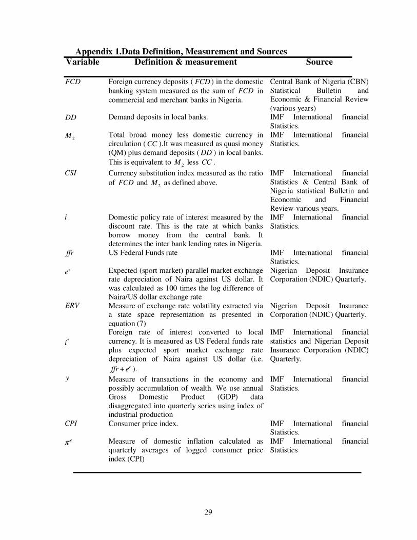
Appendix 1.Data Definition, Measurement and Sources Variable Definition & measurement Source
FCD Foreign currency deposits ( FCD ) in the domestic
banking system measured as the sum of FCD in commercial and merchant banks in Nigeria.
Central Bank of Nigeria (CBN) Statistical Bulletin and Economic & Financial Review (various years)
DD Demand deposits in local banks. IMF International financial Statistics.
2M Total broad money less domestic currency in circulation ( CC ).It was measured as quasi money (QM) plus demand deposits ( DD ) in local banks. This is equivalent to 2M less CC .
IMF International financial Statistics.
CSI Currency substitution index measured as the ratio of FCD and 2M as defined above.
IMF International financial Statistics & Central Bank of Nigeria statistical Bulletin and Economic and Financial Review-various years.
i Domestic policy rate of interest measured by the discount rate. This is the rate at which banks borrow money from the central bank. It determines the inter bank lending rates in Nigeria.
IMF International financial Statistics.
ffr US Federal Funds rate IMF International financial Statistics.
ee Expected (sport market) parallel market exchange rate depreciation of Naira against US dollar. It was calculated as 100 times the log difference of Naira/US dollar exchange rate
Nigerian Deposit Insurance Corporation (NDIC) Quarterly.
ERV Measure of exchange rate volatility extracted via a state space representation as presented in equation (7)
Nigerian Deposit Insurance Corporation (NDIC) Quarterly.
*i Foreign rate of interest converted to local currency. It is measured as US Federal funds rate plus expected sport market exchange rate depreciation of Naira against US dollar (i.e. ffr + ee ).
IMF International financial statistics and Nigerian Deposit Insurance Corporation (NDIC) Quarterly.
y Measure of transactions in the economy and possibly accumulation of wealth. We use annual Gross Domestic Product (GDP) data disaggregated into quarterly series using index of industrial production
IMF International financial Statistics.
CPI Consumer price index. IMF International financial Statistics.
eπ Measure of domestic inflation calculated as quarterly averages of logged consumer price index (CPI)
IMF International financial Statistics
30
-20
0
20
40
60
80
80 82 84 86 88 90 92 94 96 98 00 02 04
Inflation rate (annual % Changes)Grwoth Rate of M1Fical Deficits (% of GDP)
Figure 1: Some Macroeconomic Indicators in Nigeria (1980-2005)
-10
0
10
20
30
40
80 82 84 86 88 90 92 94 96 98 00 02 04
INTRATESPREADTBRMRRSavings Deposit RatePrime Lending Rate
Figure 2: Major Monetary Indicators (1980-2005) Percentages.
-40
-30
-20
-10
0
10
20
30
40
50
86 88 90 92 94 96 98 00 02 04
Real Expected exchange rate depreciationDomestic Inflation
Figure 3: Inflation Vs Real expected exchange rate depreciation (1986-2005)
31
Table 1: Summary of Reduced Form Estimation (1986.1-2005.2)
Foreign Rate Domestic Expected Change Domestic Real Currency Real of Interest Policy Rate in Exchange Rate Inflation Exchange Substitution Income Test Statistics of Interest Rate Index Volatility
( *i ) ( i ) ( ee ) ( eπ ) ( ERV ) (CSI ) ( GDP )
Cointegrating Equation
-0.0080 -0.0928 -0.0055 -0.0028 -0.0026 0.0151 0.0264
(-0.64) (-1.13) (-1.19) (-1.66) (-0.59) (1.24) (6.11)
Goodness of fit statistics Adj.R-squared 0.01 0.17 0.44 0.41 0.56 0.50 0.71
SEE 0.39 2.58 0.15 0.05 0.14 0.38 0.14
Correlation among reduced-form errors: *i 1.00 0.02 -0.04 -0.02 -0.04 0.20 -0.04
i 0.00 1.00 -0.08 0.04 -0.09 0.10 -0.09 ee 0.00 0.00 1.00 0.33 0.93 0.01 0.01 eπ 0.00 0.00 0.00 1.00 -0.05 0.14 0.43
ERV 0.00 0.00 0.00 0.00 1.00 -0.04 -0.16
CSI 0.00 0.00 0.00 0.00 0.00 1.00 0.36
GDP 0.00 0.00 0.00 0.00 0.00 0.00 1.00 Note: The model was estimated using a four-quarter lag structure per equation. The cointegrating equation presents the error correction estimate (with t-statistic in parenthesis) since the model was run through the Vector Error Correction Method. SEE stands for the standard error of the equation.
32
Table 2: Impulse Response Functions from the Reduced-Form Model
Type of
Innovations
Horizons/Quarters
Foreign Rate of Interest
( *i )
Domestic Policy Rate of Interest ( i )
Expected Change in Exchange Rate
( ee )
Domestic Inflation
( eπ )
Real Exchange Rate Volatility
( ERV )
Currency Substitution
Index (CSI )
Domestic National Income
( GDP ) 1 0.3298 -0.0479 0.0066 0.0039 0.0030 0.0605 -0.0026 3 0.1741 -0.4933 0.0015 0.0024 -0.0002 0.0247 0.0296
*iε 6 0.0165 -0.0398 0.0019 0.0072 -0.0052 0.0119 -0.0009
9 -0.0041 0.0209 -0.0022 0.0011 -0.0033 -0.0076 -0.0008 10 -0.0060 0.0110 -0.0008 -0.0002 -0.0007 -0.0015 -0.0008 1 0.0000 1.8976 -0.0152 -0.0040 -0.0108 0.0434 -0.0288 3 -0.0293 -0.0382 -0.0240 -0.0108 -0.0134 -0.0912 0.0141 iε 6 -0.0294 0.0739 0.0048 -0.0041 0.0087 0.0126 0.0013 9 0.0029 -0.0085 -0.0021 -0.0010 -0.0011 -0.0078 -0.0015 10 0.0009 -0.0198 0.0003 -0.0006 0.0008 0.0027 -0.0006 1 0.0000 0.0000 0.1147 0.0148 0.0996 -0.0310 -0.0062 3 0.1027 -0.0145 0.0069 0.0078 -0.0003 0.0037 0.0073
eeε 6 0.0095 -0.0254 0.0008 0.0040 -0.0031 0.0064 0.0020
9 -0.0025 0.0126 3.75E-05 0.0004 -0.0004 0.0006 0.0008 10 -0.0018 0.0066 -0.0007 5.62E-05 -0.0007 -0.0021 -0.0002 1 0.0000 0.0000 0.0000 0.0447 -0.0447 -0.0044 0.0529 3 -0.0126 0.1431 -0.0024 0.0016 -0.0044 0.0134 0.0065
eπε 6 0.0003 -0.0304 -0.0058 -0.0008 -0.0051 -0.0141 -0.0093 9 0.0010 0.0195 9.39E-05 6.66E-06 5.62E-05 -0.0013 0.0010 10 0.0029 -0.0030 -0.0004 -0.0001 -0.0003 -0.0003 -0.0002 1 0.0000 0.0000 0.0000 0.0000 0.0026 0.0165 0.0302 3 -0.0427 0.1173 -0.0091 0.0020 -0.0101 -0.0926 0.0209
ERVε 6 -0.0500 0.1444 0.0037 - 0.0004 0.0044 -0.0169 0.0034 9 -0.0241 0.0468 2.35E-06 -0.0012 0.0013 -0.0097 -0.0011 10 -0.0180 0.0173 0.0002 0.0009 0.0012 -0.0047 -0.0016 1 0.0000 0.0000 0.0000 0.0000 0.0000 0.2754 0.0416 3 -0.0454 0.2249 -0.0056 -0.0007 -0.0050 -0.0276 -6.14E-05
CSIε 6 -0.0140 0.0321 0.0021 -0.0026 0.0046 0.0092 -0.0009 9 0.0036 -0.0124 3.98E-05 -0.0006 0.0006 0.0017 -0.0002 10 0.0037 -0.0136 -0.0003 -0.0002 -9.5E-05 0.0001 -0.0004 1 0.0000 0.0000 0.0000 0.0000 0.0000 0.0000 0.0968 3 -0.0233 -0.0390 -0.0099 0.0038 -0.0140 -0.0133 -0.0366
GDPε 6 -1.2E-05 0.0330 -0.0038 0.0002 -0.0041 -0.0163 -0.0018
9 0.0007 -0.0037 0.0005 -0.0004 0.0009 0.0023 0.0003 10 0.0018 -0.0002 0.0004 3.42E-05 0.0004 0.0015 0.0002
Note: Entry ( ji, ) denotes the dynamic response of variable j to a one standard deviation shock in
variable i . Here, the column heads show “ i ” variables while row entries (that is,
*iε , iε , ee
ε , eπε , ERVε , CSIε , GDPε ) represent “ j” variables. All the variables corresponds to percentage
increases of the level of each variables from the baseline *i , i , ee ,
eπ , ERV , CSI , GDP.
33
Table 3: Variance Decomposition from the Reduced-Form Model Variables Horizons/
Quarters *i
ε iε eeε eπ
ε ERVε CSIε GDPε
1 100.00 0.00 0.00 0.00 0.00 0.00 0.00 3 86.71 2.08 8.05 0.22 0.82 1.77 0.34
Foreign Rate of Interest 6 81.83 2.93 8.68 0.25 3.19 2.18 0.94
( *i ) 9 80.84 2.94 8.58 0.26 4.28 2.16 0.93
10 80.73 2.94 8.57 0.27 4.40 2.17 0.93
1 0.06 99.94 0.00 0.00 0.00 0.00 0.00 Domestic Policy Rate 3 6.58 85.57 0.31 1.19 2.36 3.96 0.04
Of Interest ( i ) 6 7.79 82.52 0.87 1.75 2.76 3.92 0.40 9 7.87 82.23 0.88 1.75 2.96 3.90 0.41 10 7.87 82.22 0.88 1.75 2.96 3.90 0.41
1 0.33 1.73 97.94 0.00 0.00 0.00 0.00 Expected Change in 3 1.33 5.18 84.48 4.09 2.09 0.61 2.23
Exchange Rate 6 1.43 6.01 81.21 4.83 2.84 0.83 2.84
( ee ) 9 1.54 6.21 80.82 4.86 2.88 0.82 2.86
10 1.55 6.21 80.82 4.86 2.88 0.82 2.86
1 0.66 0.70 9.72 88.91 0.00 0.00 0.00 Domestic Inflation 3 0.89 5.48 18.83 63.09 0.63 1.28 9.80
( eπ ) 6 8.85 5.25 17.61 55.53 1.73 1.73 9.28
9 9.30 5.27 17.60 55.01 1.75 1.81 9.27 10 9.29 5.27 17.60 54.99 1.77 1.81 9.26
1 0.07 0.96 82.34 16.57 0.06 0.00 0.00 Real Exchange Rate 3 0.70 2.74 69.13 12.95 3.74 1.67 9.07 Volatility ( ERV ) 6 3.27 3.68 64.25 13.30 4.08 1.69 9.73
9 3.36 3.96 63.89 13.32 4.09 1.70 9.69 10 3.36 3.96 63.88 13.31 4.10 1.70 9.69
1 4.42 2.27 1.16 0.02 0.33 91.79 0.00 Currency Substitution 3 3.70 8.88 1.97 3.68 8.10 71.40 2.29
Index ( CSI ) 6 3.96 10.09 1.97 4.08 8.69 67.43 3.78 9 4.05 10.19 1.96 4.27 8.99 66.78 3.77 10 4.05 10.20 1.96 4.26 9.01 66.76 3.77
1 0.04 5.28 0.25 17.83 5.81 11.05 59.75 Domestic National 3 4.07 5.01 7.25 20.99 7.59 7.52 47.57 Income ( GDP ) 6 5.59 7.14 6.76 22.25 7.33 7.19 43.73
9 5.84 7.32 6.73 22.13 7.31 7.16 43.51 10 5.84 7.32 6.73 22.13 7.32 7.16 43.50
Note: Entry ( ji, ) denotes the percentage of forecast variance of variable i (that is the column
heads *iε , iε , ee
ε , eπε , ERVε , CSIε , GDPε ) at different horizons attributable to innovations in
variable j (i.e., the row entries).