MPRAMunich Personal RePEc Archive

Some new evidence on the determinantsof money demand in developing countries– A case study of Tunisia

Ousama Ben Salha and Zied Jaidi

National Engineering School of Gabes, University of Gabes, Tunisiaand International Finance Group-Tunisa, University Tunis ElManar, Tunisia , Central Bank of Tunisia, Tunisia

1. November 2013

Online at http://mpra.ub.uni-muenchen.de/51788/MPRA Paper No. 51788, posted 29. November 2013 16:47 UTC

1

Some new evidence on the determinants of money demand

in developing countries –A case study of Tunisia*

Ousama BEN SALHA

National Engineering School of Gabes, University of Gabes, TunisiaInternational Finance Group-Tunisa, University Tunis El Manar, Tunisia

Email: oussama.bensalha@isgs.rnu.tn

Zied JAIDI

Central Bank of Tunisia, TunisiaEmail: zied.jaidi@gmail.com

- Abstract -

The present paper aims at examining the money demand function in Tunisia during the period 1981-

2011. Unlike previous conventional money demand studies, the major components of real income are

considered in this paper. Using the ARDL bounds testing approach, results reveal evidence of

cointegration between broad money demand and its determinants, namely final consumption

expenditure, expenditure on investment goods, export expenditure and interest rate. In the long-run, final

consumption expenditure represents the major money demand determinant. This finding is robust to a

variety of alternative money demand specifications and estimation methods. The empirical investigation

suggests also the stability of the broad money demand function during the sample period. We conclude

that monetary policy in Tunisia should be based on a broad definition of money. Furthermore, the

estimation of the money demand function must take into account the different expenditure components

of real income.

JEL Classification: E41, E52, C22.

Keywords: Money demand, M2, expenditure components, ARDL, Tunisia.

* The views and opinions expressed in the paper are those of the authors and do not necessarily reflect the views or policies of the Central Bank of Tunisia.

2

1. Introduction

The estimation of money demand functions is a debated topic in the economic empirical

literature. Generally, the objectives consist in presenting the main determinants of the

demand for money in closed and/or open economies and checking the stability of the

money demand function. The demand for various monetary aggregates is often linked to a

scale variable representing the economic activity such as income and to a variable

representing the opportunity cost of holding money such as the domestic interest rate.

Econometrically, techniques that allow distinguishing the short-run effects from those of

the long-run, such as the error-correction modeling, are usually used.

Empirical studies have approximately covered countries of all over the world,

despite some regions received more attention than others. With regards to this point, a

review of the empirical literature shows that few studies focused on the Tunisian economy.

These include Treichel (1997), Boughrara (2001) and Simmons (1992). In line with the

majority of empirical investigations on the subject, the above studies adopted the

traditional approach, where the demand for monetary aggregates is function of a scale

variable and opportunity cost measures. However, the different components of income may

differently affect the demand for money (Ziramba 2007). Considering the impact of

aggregate income on money demand may be considered as an important methodological

limitation that may hide the impact of each expenditure component. To be more accurate

when addressing policy recommendations, it is crucial to consider the different impacts of

expenditure components in both the short-run and long-run.

Throughout this paper, we attempt to add some fresh empirical evidence to the

debate. The present case study is different from previous ones on money demand since it

estimates the short and long-run impacts of different macroeconomic components of real

income, as well as the interest rate, on the demand for M2 monetary aggregate. To the best

3

of our knowledge, no previous empirical research estimated the effects of disaggregated

real income on money demand in Tunisia.1 In addition, we use the ARDL bounds testing

approach for cointegration proposed by Pesaran et al. (2001) given its superiority to other

cointegration techniques, especially in the case of small sample studies such as the present.

The goodness of fit of the ARDL model is checked through various diagnostic tests.

Furthermore, several robustness checks, such as the inclusion of other control variables, are

implemented in order to validate our main empirical results.

The rest of the paper is structured as follows. In Section 2, we briefly survey the

empirical money demand literature that focused on Tunisia on the one hand, and that

estimated the determinants of the demand for money using various expenditure

components, on the other hand. The model specification, data, and econometric issues are

discussed in Section 3. Sections 4 and 5 present empirical findings and a number of

robustness checks, respectively. Finally, conclusions and some policy implications close

the paper.

2. Selected empirical literature

In spite of the boom in empirical works on the demand for money in developing countries

during previous years, papers focusing on the Tunisian case received a little attention.2

These few empirical studies are based on the conventional theory of money demand

relating the volume of the demanded money to a scale variable that reflects the level of

transactions in the economy (such as real income) and a variable that represents the

opportunity cost of holding money (such as the interest rate or the inflation rate). Simmons

(1992) investigates the demand for narrow money (M1) in five African countries (Congo,

Côte d'Ivoire, Mauritius, Morocco and Tunisia) using an error-correction model. Based on 1 In fact, few authors disaggregated real income when estimating money demand functions. This has been especially done by Tang (2002, 2004, 2007) in several times for some Asian economies and Ziramba (2007) for South Africa.2 Table A.2 in the Appendix summarizes some selected works on the subject.

4

annual data covering the period 1962-1989, results associated with the Tunisian case show

that the demand for money, the real income, the discount rate and the price level are

cointegrated. The author concludes also that only real income plays a statistically

significant role in explaining the long-run demand for real narrow money. Finally, real

income and inflation rate are found to be important money demand determinants in the

short-run. The same issue has been discussed by Treichel (1997) using both annual and

monthly data between 1962 and 1995 and the Johansen cointegration technique. The author

concludes that real M2 is cointegrated with real income, but not with the money market rate

or the rediscount rate. This result has been also supported by the error-correction model,

since the error-correction term is negative and statistically significant. The estimated

income elasticity over the whole period is about 0.80. It has been also shown that the

cointegrating relationship was stable, especially over the period 1962-1990. The income

elasticity over that period is twice higher than the one associated with the entire period

(1962-1995). The author attributes these findings to the reduced demand for M2 over the

period 1990-1995, due essentially to the introduction of treasury bills in 1990. These results

are confirmed econometrically by using quarterly data over the period 1990-1995. A

cointegration relationship between the demand for M2 money, income and the treasury bill

rate is detected. However, the income elasticity dramatically falls and is lower than the one

found over the whole period.

Arize and Shwiff (1998) estimate a money demand function in 25 developing

countries using annual data covering the period 1960-1990 in the case of Tunisia. Money

demand functions were augmented by two variables measuring the exchange rate: the

official one and the black market one. Empirical results suggest that real broad money

demand is cointegrated with real income, interest rate, inflation rate and the black market

rate or the official exchange rate. The same results are revealed for the case of narrow

5

money. The dynamic OLS technique suggests that real income, interest rate and either

official exchange rate or black market exchange rate are the main long-run determinants of

money demand. In addition, the long-run income elasticity is greater than the unity in all

cases. Finally, based on Fair (1987) and Davidson and MacKinnon (1981) procedures, the

authors conclude that the introduction of the black market exchange rate is more relevant

than the official exchange rate in developing countries.

Arize et al. (1999) focus on the same issue by estimating the money demand

function in 12 developing countries, including Tunisia. Besides the introduction of

traditional determinants of money demand, such as income and interest rate, the authors use

variables reflecting the extent of openness, such as the exchange rate, the exchange rate

variability and the foreign interest rate. Empirical findings reveal that a long-run

equilibrium relationship exists between either real M1 and real M2 balances and their

determinants. With respect to real M2 demand, the estimated long-run parameters are about

1.25, -0.01 and -0.03 for real income, interest rate and exchange rate variability,

respectively. Boughrara (2001) sheds light on the impact of structural reform on broad

money demand function in Tunisia. The study employed quarterly data covering the period

between the first quarter of 1987 and the second quarter of 1992. It has been shown that the

demand for M2 monetary aggregate is cointegrated with real income, the treasury bill

interest rate and the special deposits interest rate. In the long-run, all these variables affect

the demand for money. The long-run income elasticity is found to be close to the unity and

is higher than the one of the short-run. The Chow test and the recursive regression method

suggest that the money demand function in Tunisia is stable over the sample period under

study.

An important methodological shortcoming arising from the empirical literature cited

above consists in the fact that no study attempted to estimate the impact of various

6

expenditure components on money demand in Tunisia. In fact, it is crucial to check the

impact of each component of gross domestic product on the demand for money. This will

allow determining which of them affect more the demand for money. A survey of the

empirical literature suggests that few papers made such a disaggregation when estimating

the demand for money function.

Tang (2002) focuses on the determinants of money demand in Malaysia using the

ARDL bounds testing approach suggested by Pesaran et al. (2001). The author finds

evidence that the demand for M3 monetary aggregate and its determinants are cointegrated.

The CUSUM and CUSUMSQ show that the relationship is stable over time. The estimated

long-run coefficients are about 0.98 for final consumption expenditure, -0.48 for

expenditure on investment goods, 0.94 for expenditure on export of goods and services, -

1.39 for exchange rate and 0.03 for the interest rate. In the short-run, factors that affect the

money demand are exports expenditure and the exchange rate. The study confirms that the

various demand components exert different impacts on the demand for money and

concluded the bias of using single real income variable in the money demand function.

Tang (2004) estimates a money demand function based on Japanese quarterly data covering

the period between the first quarter of 1973 and the second quarter of 2000. The author

shows that broad money, as defined by the sum of M2 monetary aggregate and certificates

of deposit, was stable during that period. The study confirms the existence of a long-run

relationship between the demand for broad money, final consumption expenditure,

expenditure on investment goods, exports expenditure, deposit rate and government bond

yield rate. In the long-run, expenditure on investment goods is the most important long-run

determinant of Japanese broad money demand with elasticity equal to 1.07. However, in the

short-run, all regressors are significant at 10% level.

7

Ziramba (2007) estimates a money demand function based on different components

of real income in South Africa over the period 1970-2005. The research is based on the

demand of M1, M2 and M3 monetary aggregates. Even if long-run results depend on the

used monetary aggregate, the interest rate and the expenditure on investment goods are

found to be the common determinants of the demand for all monetary aggregates. The last

article that disaggregated real income according to expenditure components is the one of

Tang (2007) studying the case of five Southeast Asian countries (Malaysia, Philippines,

Thailand, Indonesia and Singapore). The study is based on annual data with sizes between

34 and 45 observations. Empirical results divulge that the demand for M2 balances is

cointegrated with its determinants only for three countries, Malaysia, Philippines, and

Singapore. For two of these countries, final consumption expenditure and exports

expenditure are found to be long-run determinants of money demand, while interest rate

exerts negative and significant impact only in The Philippines. The CUSUM and CUSUM

of squares tests suggest the stability of the estimated parameters. The author concludes that

M2 is the right targeted instrument to be considered to conduct monetary policy in

Philippines, Singapore and Malaysia.

3. Empirical issues

3.1. Model specification and data

Generally, the demand for money is expressed in terms of a scale variable, such as the real

income, and a variable representing the opportunity cost of holding money, such as the

interest rate or the inflation rate. In the money demand function, the real domestic income

and the opportunity cost of holding money are both important variables, because the

efficacy of the monetary policy is highly dependent on the responsiveness of their

elasticities. The demand for money is generally of the following form:

8

M

= f(y, i)P

where real money demand (M/P) depends on real income (y) and a variable

measuring the opportunity cost of holding money (i). Following Tang (2002, 2004 and

2007) and Ziramba (2007), the current study decomposes real income into its components,

namely investment, consumption and export expenditures. The decomposition gives the

following money demand function:

ln ln ln lnt t t t t t40 1 2 3γ γ γ γ γ εM2 = + FCE + EIG + EX + i +

where M2 , FCE, EIG, EX and i stand for the demand for broad money, final

consumption expenditure, expenditure on investment goods, expenditure on total exports of

goods and services and the interest rate, respectively. tε is the error term and ln is the

natural logarithmic transformation. All variables introduced in Equation (2) are in constant

local currency. As in Narayan and Narayan (2008) and Avouyi-Dovi et al. (2011), the

interest rate is not in the logarithmic form. Based on theory, it is expected that the signs

of 1 , 2 and 3 to be positive, while 4 to be negative. The study is based on annual data

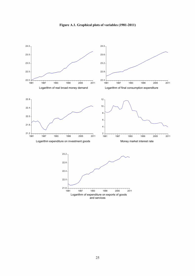
ranging between 1981 and 2011. The use of annual time series is essentially due to

unavailability of long period quarterly data, particularly for the various components of real

domestic income. Full definitions and sources of time series introduced in the empirical

investigation are given in Table A.1 in the Appendix, while plots of time series introduced

in Equation (2) are presented in Figure A.1 in the Appendix.

The choice of M2 monetary aggregate to carry out this study is not arbitrary.

Bahmani-Oskooee and Techaratanachai (2001) suggest that the use of the M2 monetary

aggregate is more appropriate in formulating monetary policy. In addition, the Central Bank

of Tunisia considers the M2 monetary aggregate as an intermediate target when conducting

(1)

(2)

9

the monetary policy (Boughrara, 2001; Mohamed Sghaier and Abida, 2013). Treichel

(1997) indicates that the broad money is a controllable and operational target in Tunisia and

thus, it may be considered as an intermediate target.3 Finally, as indicated in Table A.2, four

studies out of five focusing on Tunisia used the M2 monetary aggregate as a dependant

variable when estimating the money demand function.

3.2. The econometric methodology

Compared to conventional cointegration techniques such as the Engle-Granger two-step

technique (1987) and the Johansen and Juselius technique (1990), the ARDL bounds testing

approach introduced originally by Pesaran and Shin (1999) and then extended by Pesaran et

al. (2001) presents some major advantages. First, the conventional techniques of

cointegration require that variables introduced in the regression are integrated of order one,

while the ARDL bounds testing approach may be implemented regardless of the stationary

properties of variables (integrated of order zero, order one or fractionally integrated).

Accordingly, this technique eliminates the uncertainty associated with the order of

integration (Ben Salha, forthcoming). Second, it may be applied in small sample sizes,

whereas the Engle-Granger or the Johansen and Juselius procedure is not consistent for

relatively small samples (Duasa, 2007; Akpan, 2011). The current study is based on annual

data ranging between 1981 and 2011, which makes the ARDL approach more suitable.

Bahmani-Oskooee and Gelan (2008) report that the ARDL bounds testing approach is the

most appropriate technique for the estimation of money demand functions in developing

countries. Third, it provides unbiased long-run estimates and valid t statistics even if some

of regressors are endogenous (Paul et al. 2011; Odhiambo 2009). Finally, Hammoudeh and

Sari (2011) suggest that when using the ARDL approach, the derived error-correction

model is obtained through a simple linear transformation. In order to implement of the 3 Arize and Shwiff (1998) conclude also that M2 is preferred to M1 when estimating the money demand function in 25 developing economies, including Tunisia.

10

Δ Δ Δ Δ Δ

Δ

ln ln ln ln ln

ln ln nln l

0

t-1 t-1 t-1 t-1

t t- j t- t- t-

t-

p p p p

j=1 =0 =0 =0p

1 2 3 4 5 t-1 t=0

k m n

ih

nk mjk m n

hh

ψ λ

η

α

δ δ δ δ δ

M2 = + φ M2 + FCE + EIG + EX

+ i + M2 + FCE + EIG + EX + +ε

ARDL bounds testing approach, the money demand function presented in Equation (2) is

transformed as follows:

Where is the first difference operator. To examine the evidence for a long-run

relationship between lnM2t, lnFCEt, lnEIGt, lnEXt and i, Pesaran et al. (2001) propose the

bounds test conducted based on the Wald test (F-test). The F-test is a test where the null

hypothesis is the absence of cointegration among variables against the presence of

cointegration as an alternative hypothesis, both denoted as:

1 2 3 4 5: = = = = = 00H i.e., the absence of cointegrating relationships

1 1 2 3 4 5: 0H i.e., the existence of cointegrating relationships

It is important to note that the asymptotic distribution of the F-statistic is not

standard under the null hypothesis of no cointegration, irrespective of whether the

explanatory variables are purely I(0) or I(1). According to Narayan and Narayan (2005), the

two critical bounds values (lower and upper) computed by Pesaran and Pesaran (1997)

depend on three main criteria: (i) The integration order of explanatory variables (I(0) or

I(1)); (ii) The number of explanatory variables; and (iii) The inclusion of only an intercept

or of an intercept and a trend. The decision on the existence of cointegration or not is based

on the comparison between the F-statistic and the bounds critical values. For instance, for a

given significance level (1%, 5% or 10%), if the computed F-statistic is higher than the

upper critical bounds value then the null hypothesis for no cointegration is rejected. In the

case when the F-statistic lies between the upper and lower critical values, no conclusive

decision on the existence of cointegration would be advanced. Finally, if the F-statistic falls

(3)

11

below the lower critical bounds value, the null hypothesis of no cointegration cannot be

rejected. Once a cointegrating relationship between the demand for money and its

determinants is found, we estimate the long-run elasticities using the following equation:

ln ln ln ln

ln t

t t - j t- j t -

t- jt-

qu r

0 3j=1 j=0 j=0

s v

j=0 j=0

j

j

1

4

2

ν5

M2 γ γ M2 γ FCE γ EIG

γ EX γ i

= + + +

+ + +

Finally, the estimation of the short-run dynamics is done by estimating the error-

correction model associated with the ARDL model. It assumes the following form:

Δ Δ Δ Δ

Δ Δ

ln ln ln ln

ln tt -1

t t- j t - j t-

t- jt-

n n n

0 3j=1 j=0 j=0

n n

j=0 j=0

j

j

1

4 6

2

+ ν5

M2 γ γ M2 γ FCE γ EIG

γ EX γ i γ ε

= + + +

+ + +

t-1ε is the one period lagged error-correction term. This term measures the speed of

adjustments towards the long-run equilibrium relationship if short-run shocks occurred. In

addition, a negative and statistically error-correction term confirms the results of the F-test

concerning the existence or not of cointegration between variables (Bahmani-Oskooee and

Rehman, 2005).

4. Empirical findings

4.1. Integration and cointegration analysis

Before testing the presence of long-run relationships between the demand for M2 balances

and their determinants, we have to study the stationary properties of variables introduced in

the model. In fact, even if the ARDL bounds testing technique allows testing the presence

of cointegration although variables are of different order of integration, it is not possible to

(4)

(5)

12

implement it if some of them are integrated of order two or above.4 In Table 1, we present

results of the Phillips-Perron and Dickey-Fuller GLS unit root tests.

The two unit root tests are performed with an intercept and with an intercept and a

trend term. The Phillips-Perron unit root test indicates that all variables are not stationary in

level and stationary in first difference. Results of the Dickey-Fuller GLS test confirm also

those of the Phillips-Perron test. Thus, variables introduced in the model are all integrated

of order one. Given that no variable is integrated of an order higher than one, the ARDL

bounds testing approach may be applied to test the existence of cointegration relationships.

In Table 2, we report F-statistics calculated when each variable is taken as a dependent

variable, which means that we have five different specifications. As mentioned previously,

the bounds testing approach to cointegration involves the comparison of the F-statistics

against the computed critical value bounds. Results suggest that when the real money

demand is considered as the dependent variable, the computed F-statistic exceeds the upper

bound critical value at the 1% significance level.

4 This is due to the fact that there is no provision for I(2) in the critical values for bounds testing approach.

Table 1. Unit root tests results

VariablePhillips-Perron Dickey-Fuller GLS

intercept intercept and trend intercept intercept and trendLevellnM2 1.530 -1.069 0.543 -1.416lnFCE -0.036 -1.638 -1.216 -1.478lnEIG -0.028 -2.275 -0.589 -1.853lnEX -0.915 -1.505 0.283 -1.556i -0.376 -2.023 -0.281 -1.747First differencelnM2 -3.945*** -4.234** -4.007*** -4.428***

lnFCE -2.847* -2.511 -2.870*** -2.971*

lnEIG -3.486** -3.561* -6.412*** -3.497**

lnEX -4.805*** -6.448*** -3.392*** -4.504***

i -4.316*** -4.413*** -4.387 -4.583***

Notes: The Schwarz information criterion and the Newey-West Bandwidth method using Bartlett kernel are used to select the optimal lag length for the FF-GLS and PP unit root tests, respectively. The null hypothesis is the existence of unit root. ***, ** and * denote the rejection of the null hypothesis at 1%, 5% and 10% significance levels, respectively.

13

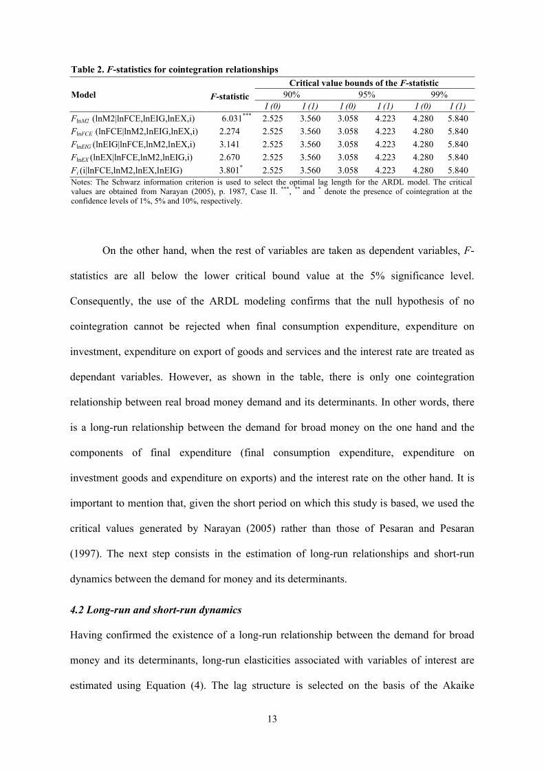
Table 2. F-statistics for cointegration relationships

Model F-statistic

Critical value bounds of the F-statistic90% 95% 99%

I (0) I (1) I (0) I (1) I (0) I (1)FlnM2 (lnM2|lnFCE,lnEIG,lnEX,i) 6.031*** 2.525 3.560 3.058 4.223 4.280 5.840

FlnFCE (lnFCE|lnM2,lnEIG,lnEX,i) 2.274 2.525 3.560 3.058 4.223 4.280 5.840

FlnEIG (lnEIG|lnFCE,lnM2,lnEX,i) 3.141 2.525 3.560 3.058 4.223 4.280 5.840

FlnEX (lnEX|lnFCE,lnM2,lnEIG,i) 2.670 2.525 3.560 3.058 4.223 4.280 5.840

Fi (i|lnFCE,lnM2,lnEX,lnEIG) 3.801* 2.525 3.560 3.058 4.223 4.280 5.840Notes: The Schwarz information criterion is used to select the optimal lag length for the ARDL model. The critical values are obtained from Narayan (2005), p. 1987, Case II. ***, ** and * denote the presence of cointegration at the confidence levels of 1%, 5% and 10%, respectively.

On the other hand, when the rest of variables are taken as dependent variables, F-

statistics are all below the lower critical bound value at the 5% significance level.

Consequently, the use of the ARDL modeling confirms that the null hypothesis of no

cointegration cannot be rejected when final consumption expenditure, expenditure on

investment, expenditure on export of goods and services and the interest rate are treated as

dependant variables. However, as shown in the table, there is only one cointegration

relationship between real broad money demand and its determinants. In other words, there

is a long-run relationship between the demand for broad money on the one hand and the

components of final expenditure (final consumption expenditure, expenditure on

investment goods and expenditure on exports) and the interest rate on the other hand. It is

important to mention that, given the short period on which this study is based, we used the

critical values generated by Narayan (2005) rather than those of Pesaran and Pesaran

(1997). The next step consists in the estimation of long-run relationships and short-run

dynamics between the demand for money and its determinants.

4.2 Long-run and short-run dynamics

Having confirmed the existence of a long-run relationship between the demand for broad

money and its determinants, long-run elasticities associated with variables of interest are

estimated using Equation (4). The lag structure is selected on the basis of the Akaike

14

information criterion. Results are reported in Table 3. Final consumption expenditure and

the interest rate are found to be the only significant variables that explain the long-run

demand for M2. The estimated long-run elasticities of the determinants of money demand

are 1.861 for final consumption expenditure and -0.056 for interest rate.

Table 3. Long-run coefficients of the money demand function

Regressor Coefficient Standard error p-valuelnFCEt 1.862*** .362 .000lnEIGt -.313 .239 .204lnEXt -.356 .209 .105it -.056* .030 .078Constant -4.862 4.058 .244

Notes: ***, ** , * indicate statistical significance at 1%, 5 % and 10% level, respectively.

The elasticity on final consumption expenditure is higher than the unity, which is

not surprising since final consumption expenditure represents the major component of GDP

in Tunisia. The demand for M2 monetary aggregate is essentially due to private

consumption expenditure and government consumption expenditure. With regards to the

interest rate, the statistical significance and the magnitude of its coefficient point out that its

effect on real money demand is weak. Finally, expenditure on investment goods and

expenditure on export of goods and services exert no impacts on the demand for money in

the long-run.

Given the existence of a long-run relationship between the money demand and its

determinants, we proceed to the estimation of the short-run dynamics, via the

implementation of the error-correction model. The deviations from the long-run

relationship may be due to the occurrence of shocks in the short-run. The use of the error-

correction model allows checking the short-run elasticities and measuring the speed of

adjustments to the long-run equilibrium via the error-correction term. In addition, a

negative and statistically significant coefficient is an indicator on the existence of

15

cointegration. Panel A of Table 4 reports the estimated error-correction representation for

the ARDL equation.

Table 4. Short-run coefficients of the money demand function and validation tests

Panel A : Error correction model representationRegressor Coefficient Standard error p-valueΔlnFCEt -.040 .301 .894ΔlnEIGt .219** .088 .021ΔlnEXt .069 .114 .549Δit -.015*** .004 .003ECM t-1 -.270** .104 .016Constant -2.554 1.862 .185Panel B: Diagnostic tests of the underlying the ARDL modelLM test of residual serial correlation 1.161 (.281)Normality test .508 (.775)Ramsey Reset test 1.024 (.311)Heteroscedasticity test .232 (.630)R-squared .660Notes: LM test is the Lagrange Multiplier test of residual serial correlation; Normality test is based on skewness and kurtosis, Ramsey Reset test is the Ramsey test for omitted variables/functional form and the Heteroscedasticity test is based on the regression of squared residuals on squared fitted values. ***, ** , * indicate statistical significance at 1%, 5 % and 10% level, respectively

As can be seen, the error-correction term is negative and statistically significant at

5% level, confirming the results of the bounds testing procedure and indicating that the

volume of money demand and its determinants cannot diverge systematically from a long-

run equilibrium position. In this context, the value of the error-correction term is relatively

low, indicating that nearly 27% of the disequilibria in the demand for M2 monetary

aggregate due to previous shocks adjust back to the long-run equilibrium in the current

year. Regarding the components of real income, only the final expenditure on investment is

found to influence the demand for M2 and its sign is as expected with an estimated

elasticity of about 0.219. The coefficient on the interest rate is also statistically significant

and is negative. Panel B of Table 4 presents some diagnostic tests that aim at measuring the

adequacy of the estimated error-correction model. Results reveal that there is no serial

correlation, non normality and heteroscdasticity in the residuals. The Ramsey RESET test

confirms also the correct functional form of the model. Tang (2004) reports that the RESET

16

test allows detecting specification errors, such as simultaneous equation issues, omitted

variables and serially correlated disturbances. The R-squared indicates that about 66% of

variations in the demand for M2 monetary aggregate is explained by regressors introduced

in the specification.

5. Robustness checks

The present section aims at considering some robustness checks of our main analysis. This

will allow us gauging the sensitivity of previous results with respect to many empirical

issues such as the choice of econometric techniques or control variables. Three robustness

and sensitivity checks linked to the estimation of the long-run parameters are conducted.

First, we re-estimate the long-run parameters using the fully-modified ordinary least

squares (FMOLS) and the dynamic ordinary least squares (DOLS). Second, we introduce

additional control variables to our baseline specification and re-estimate the long-run

parameters associated with the modified money demand function. Finally, we check the

stability of long-run parameters using the cumulative sum of recursive residuals (CUSUM)

and the cumulative sum of squares of recursive residuals (CUSUMSQ) tests.

5.1. Further estimates of long-run parameters

As reported by Narayan and Narayan (2004), the FMOLS technique advocated by Phillips

and Hansen (1990) has two main advantages. On the one hand, it eliminates the sample

bias. On the second hand, it corrects for endogeneity and serial correlation effects. With

regards to the DOLS technique developed by Stock and Watson (1993), it essentially

avoids to problems related to small sample bias and simultaneity.5 In table 5, we present

long-run results using the dynamic OLS (Panel A) and fully modified OLS (Panel B).

5 According to Stock and Watson (1993), the problem of simultaneity and small sample bias is resolved by regressing the dependant variable on explanatory variables in levels, leads and lags of the explanatory variables.

17

Table 5. Long-run coefficients of the money demand function - Further estimates

Panel A: Dynamic OLS estimatesRegressor Coefficient Standard error p-valuelnFCEt 1.323*** .298 .001lnEIGt -.043 .221 .848lnEXt -.052 .146 .726it -.034** .011 .013Constant -5.328* 2.432 .005Panel B: Fully Modified OLS estimatesRegressor Coefficient Standard error p-valuelnFCEt 1.762*** .194 .000lnEIGt -.013 .110 .905lnEXt -.265** .107 .020it .003 .010 .737Constant -11.790*** 1.994 .000Notes: ***, ** , * indicate statistical significance at 1%, 5 % and 10 % level, respectively.

Findings from the DOLS technique are similar to those of the ARDL approach since

final consumption expenditure and interest rate have positive and negative coefficients,

respectively, and are statistically significant. The use of the FMOLS technique partially

corroborates with those found previously. The consumption and exports components of

GDP are the only significant explanatory variables. Finally, it is important to note that the

elasticity associated with consumption is higher than the unity (1.323 and 1.762 using the

DOLS and the FMOLS, respectively, against 1.862 using the ARDL). Consequently, a

common feature that arises from the use of the DOLS and FMOLS techniques is that final

consumption is positively linked to the demand for broad money in Tunisia, a result similar

to the one found when the ARDL approach is employed.

5.2. Additional control variables

The second exercise we implement in order to check the robustness of our main analysis is

the introduction of other control variables that appear to be potential explanatory variables

of the demand for money. First, the nominal effective exchange rate is included in the

money demand function (Panel A of Table 6) as a measure of currency substitution. As

reported by Debson and Ramlogan (2001), the exchange rate is usually introduced in the

money demand function in order to capture the degree of openness of the economy.

18

Second, as suggested by many authors, the inflation rate could be employed as a second

measure of the opportunity cost of holding money (Bahmani-Oskooee and Gelan, 2008;

Kumar, 2011). For example, Baharumshah et al. (2009) advance that for the case of China

as a developing country, using the interest rate or the inflation rate as a measure of the

opportunity cost of holding money is a difficult task. Treichel (1997) used both the inflation

rate and the interest rate when estimating the money demand function in Tunisia. In Panel

B of Table 6, the inflation rate as well as the interest rate are introduced, whereas in Panel

C, only the inflation rate is maintained. The estimation of long-run parameters is based on

the ARDL approach. Before estimating long-run coefficients, we checked the existence of

cointegration relationships between broad money demand, the different components of

income, interest rate and the newly introduced control variables.

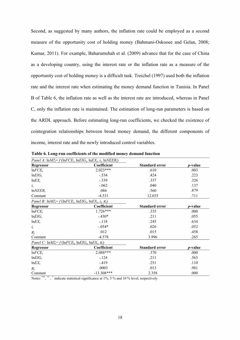
Table 6. Long-run coefficients of the modified money demand function

Panel A: lnM2t= f (lnFCEt, lnEIGt, lnEXt, it, lnNEERt)Regressor Coefficient Standard error p-valuelnFCEt 2.023*** .610 .003lnEIGt -.534 .424 .223lnEXt -.339 .337 .326it -.062 .040 .137lnNEERt .086 .560 .879Constant -4.531 12.035 .711Panel B: lnM2t= f (lnFCEt, lnEIGt, lnEXt, it, πt)Regressor Coefficient Standard error p-valuelnFCEt 1.726*** .335 .000lnEIGt -.430* .211 .055lnEXt -.118 .245 .634it -.054* .026 .052

πt .012 .015 .458Constant -4.578 3.996 .265Panel C: lnM2t= f (lnFCEt, lnEIGt, lnEXt, πt)Regressor Coefficient Standard error p-valuelnFCEt 2.088*** .370 .000lnEIGt -.124 .211 .563lnEXt -.419 .251 .110

πt .0003 .013 .981Constant -13.308*** 2.358 .000Notes: ***, ** , * indicate statistical significance at 1%, 5 % and 10 % level, respectively

19

The ARDL testing approach suggests that for Panel A and Panel B, real broad

money demand and its determinants are cointegrated at 5% and 1% statistical levels,

respectively.6 When we use only the inflation rate as an opportunity cost measure, no

cointegration relationship is found, but we keep it in the analysis.7 Turning to the estimation

of the long-run coefficients, results reveal that the introduction of the nominal effective

exchange rate (Panel A) or the inflation rate (Panels B and C) does not affect our main

conclusion: the final consumption expenditure is the most important determinant of broad

money demand.8 Coefficients associated with final consumption expenditure are significant

at 1% level in all cases and are close to those obtained in the baseline specification. In

addition, when introduced in the regression, the inflation rate exerts no effect on the

demand for money in the long-run. According to Boughrara (2001), the inflation rate has

been stable in Tunisia over the past decades and consequently he did not introduce it in the

money demand function. Mixed with previous results, this finding confirms the idea that

the demand for M2 monetary aggregate does not depend on variables measuring the

opportunity cost of holding money. Similar results are found for the nominal effective

exchange rate, which may be explained by the fact that the detention of foreign currencies

is highly regulated in Tunisia. The substitution between domestic and foreign currencies is

not an easy operation in the case of appreciation or depreciation of the exchange rate.

6 FlnM2 (lnM2|lnFCE,lnEIG,lnEX,i,lnNEER) is equal to 4.648 while the Narayan’s (2005) critical values at 5% statistical level are 2.910 and 4.193, whereas FlnM2 (lnM2|lnFCE, lnEIG, lnEX,i,π) is about 5.820 while the critical values at 1% statistical level are 4.134 and 5.761.7 The associated F-statistic is equal to 3.102. It ranges between the 5% and 10% upper and lower bounds, so that we cannot decide on the existence of cointegration. Bahmani-Oskooee and Rehman (2005) and Tang (2007) point out that the F-statistic remains preliminary when testing the existence of cointegration and that the coefficient on the lagged error-correction term is a more efficient tool. Kremers et al. (1992) advances that the error-correction term is more powerful when testing the existence of cointegration. The results of the error-correction model (not reported here because of space constraints but are available upon request from the authors) suggest that the coefficient on the lagged error-correction term is negative (-.348) and statistically significant at 5% level.8 Even when the real effective exchange rate is used instead of the nominal effective exchange rate, the demand for money and its determinants remain cointegrated. In addition, the final consumption expenditure is the only determinant of money demand with a long-run elasticity of about 2.057.

20

-20

-10

0

10

20

1982 1990 1998 2006 2011

-0.4

-0.2

0.0

0.2

0.4

0.6

0.8

1.0

1.2

1.4

1982 1990 1998 2006 2011

5.3. Long-run parameters stability

Based on results found in the previous section, a long-run relationship between the demand

for broad money and its determinants exists. In addition, final consumption expenditure is

found to be the main long-run determinant of broad money demand. The issue that arises is

whether this long-run relationship is stable or not over time. This is an important point

since monetary policies may not be designed and executed if the studied relationship is

unstable (Dobnik, 2013; Hansen and Kim, 1995).

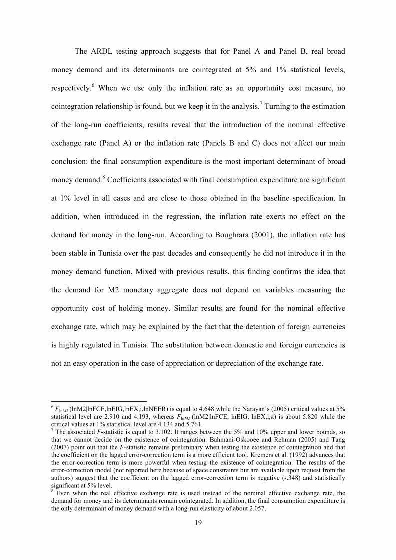
Figure 1. Plots of (a) cumulative sum of recursive residuals (CUSUM) and (b) cumulative sum of squares of recursive residuals (CUSUMSQ) statistics.

(a) Plot of Cumulative Sum of Recursive Residuals

(b) Plot of Cumulative Sum of Squares of Recursive Residuals

21

Treichel (1997) indicates that the effectiveness of the money demand function in

terms of policy recommendations depends primary upon its stability. A simple and efficient

way to test long-run parameters stability, as advanced by Pesaran and Pesaran (1997), is the

use of the CUSUM and CUSUM of squares tests proposed by Brown et al. (1975). These

two statistics are updated recursively and plotted against break points in the studied

relationship. The decision is generally made graphically: if plots of the CUSUM and

CUSUM of squares statistics do not cross pairs of 5% critical lines, the relationship is

considered as stable. A graphical presentation of these two tests (based on the ARDL

estimates) is provided in Figure 1. As is evident from plots, there is no movement outside

the critical lines, suggesting the absence of any structural instability in the estimated ARDL

models during the investigated period.

6. Conclusion and policy implications

The main aim of this study is to examine the long and short-run determinants of broad

money demand Tunisia. Unlike the majority of previous studies on the subject, the current

one considers various components of real income. It splits the domestic income into its

main components such as consumption, investment and export expenditures. Using a

relatively recent cointegration technique, the ARDL bounds testing approach, we found

evidence of the existence of long-run cointegration relationship between M2 balances, the

various components of real income and the interest rate. It emerges also that final

consumption expenditure and interest rate are the only variables that affect the real money

demand in the long-run. However, the impact of final consumption expenditure is higher

than the one of the interest rate. These findings are robust to a variety of money demand

specifications and estimation methods. Even when we introduced the nominal effective

exchange rate and the inflation rate in the money demand function, our main conclusions

22

remain valid. In the short-run, both expenditure on investment goods and the interest rate

affect the demand for money. With respect to the stability of the money demand function,

results based on the CUSUM and CUSUM of square tests suggest that the estimated

parameters are stable over the studied period. These findings have important implications

on policy formulation in Tunisia. An expenditure-switching or expenditure-reducing policy

on final consumption can be adopted in order to act on the demand for money. The negative

long-run elasticity on the interest rate means that it can be used to influence monetary

policy in Tunisia. However, the coefficient is too small. This implies that if the demand for

broad money is considered as a monetary target, it will take quite a large change in the

interest rate before inducing the desired change in the M2 demand.

23

Appendix

Table A.1. Variable derivations and data sources

Variable Description SourceBroad money (M2) Nominal values of M2 are deflated

by the consumer price index (1990=100).

World Development Indicators, World BankTunisian National Institute of Statistics.

Final consumption expenditure (FCE)

The sum of household consumption and general government consumption at constant prices 1990 (1990=100) (in millions Tunisian dinars).

World Development Indicators, World Bank

Expenditure on investment goods (EIG)

The gross fixed capital formation at constant prices 1990 (1990=100) (in millions Tunisian dinars).

World Development Indicators, World Bank

Expenditure on exports of goods and services (EX)

_World Development Indicators, World Bank

Interest rate (i) Money market interest rate International Financial Statistics, IMF

Inflation rate (π)_

Tunisian National Institute of Statistics

Nominal effective exchange rate (NEER) _

International Financial Statistics, IMF

Real effective exchange rate (REER) _

International Financial Statistics, IMF

24

Table A.2. Survey of selected empirical works

Study Monetary aggregate Countries Period TechniqueDeterminants of money demand

♯ ‡

Short-run Long-run

1st group: Studies focusing on Tunisia

Simmons (2000) M1 5 African countries, including Tunisia

1962-1989 Error-correction model

Income, inflation Real income

Treichel (1997) M2, M4 Tunisia 1962-1995 Johansen _ Real income, treasury bill rate

Arize and Shwiff (1998) M1, M2 25 Developing countries, including Tunisia

1960-1990 Johansen _ Real income, interest rate, black market exchange rate, official exchange rate.

Arize et al. (1999) M1, M2 12 Developing countries, including Tunisia

1964-1996 Johansen _ Real income, exchange rate, exchange rate variability, inflation rate.

Boughrara (2001) M2 Tunisia 1987-1992 Engle-Granger, Shin procedure

Real income Real income, treasury bills interest rate, special deposits interest rate

2nd group: Studies decomposing real income

Tang (2002) M3 Malaysia 1973-1998 ARDL Export expenditures, exchange rate. Final consumption expenditure, expenditure on investment goods, expenditure on exports, exchange rate, interest rate.

Tang (2004) M2 Japan 1973-2000 Johansen and ARDL Final consumption expenditure, expenditure on investment goods, expenditure on exports, government bond yield rate, deposit rate.

Expenditure on investment goods, deposit rate.

Tang (2007) M2 Five Southeast Asian countries Varies according to the country

Final consumption expenditure (1), expenditure on exports (3), inflation rate (1), exchange rate (1).

Final consumption expenditure (2), expenditure on exports (2), inflation rate (1).

Ziramba (2007) M1, M2 and M3 South Africa 1970-2005 ARDL Final consumption expenditure, interest rate.

Expenditure on investment goods, final consumption expenditure, expenditure on exports, interest rate, government bond yield rate, exchange rate.

Notes: ♯

For the first group, if the study focuses on a set of countries, we only report the determinants of money demand in Tunisia. ‡

Figures in brackets indicate the number of countries in which the associated regressor affects the money demand.

25

22.0

22.5

23.0

23.5

24.0

1981 1987 1993 1999 2005 201122.4

22.8

23.2

23.6

24.0

1981 1987 1993 1999 2005 2011

21.6

22.0

22.4

22.8

23.2

1981 1987 1993 1999 2005 2011

21.2

21.6

22.0

22.4

22.8

1981 1987 1993 1999 2005 20112

4

6

8

10

12

1981 1987 1993 1999 2005 2011

Figure A.1. Graphical plots of variables (1981-2011)

Logarithm of real broad money demand Logarithm of final consumption expenditure

Logarithm expenditure on investment goods Money market interest rate

Logarithm of expenditure on exports of goods and services

26

References

Akpan, U.F., 2011. Cointegration, causality and Wagner's hypothesis: time series evidence

for Nigeria, 1970-2008. Journal of Economic Research, 16(1), 59-84.

Arize, A.C., Malindretos, J., Shwif, S.S., 1999. Structural breaks, cointegration, and speed

of adjustment Evidence from 12 LDCs money demand. International Review of

Economics and Finance, 8(4), 399-420.

Arize, A.C., Shwif, S.S., 1998. The appropriate exchange-rate variable in the money

demand of 25 countries: an empirical investigation. North American Journal of

Economics and Finance, 9(2), 169-185.

Avouyi-Dovi, S. Drumetz, F. Sahuc, J.G., 2011. The money demand function for the Euro

area: some empirical evidence. Bulletin of Economic Research, 64(3), 377-392.

Baharumshah, A.Z., Mohd, S.H., Masih, A.M.M., 2009. The stability of money demand in

China: evidence from the ARDL model. Economic Systems, 33(3), 231-244.

Bahmani-Oskooee, M. Gelan, A., 2008. How stable is the demand for money in African

countries? Journal of Economic Studies, 36(3), 216-235.

Bahmani-Oskooee, M., Rehman, H., 2005. Stability of the money demand function in

Asian developing countries. Applied Economics, 37(7), 773-792.

Bahmani-Oskooee, M., Techaratanachai, A., 2001. Currency substitution in Thailand.

Journal of Policy Modeling, 23(2), 141-145.

Ben Salha, O., Forthcoming. Economic globalization, wages and wage inequality in

Tunisia: an ARDL bounds testing approach. Review of Middle East Economics and

Finance, forthcoming.

Boughrara, A., 2001. Money demand in Tunisia during the reform period. Savings and

Development, 25(2), 117-137.

27

Brown, R.L., Durbin, J., Evans, J.M., 1975. Techniques for testing the constancy of

regression relationships over time. Journal of the Royal Statistical Society, Series B

(Methodological), 37(2), 149-192.

Davidson, R., Mackinnon, J.G., 1981. Several tests for model specification in the presence

of alternative hypotheses. Econometrica, 49(3), 781-793.

Debson, S. Ramlogan, C., 2001. Money demand and economic liberalization in a small

open economy-Trinidad and Tobago. Open Economies Review, 12(3), 325-339.

Dobnik, F., 2013. Long-run money demand in OECD countries: what role do common

factors play? Empirical Economics, 45(1), 89-113.

Duasa, J., 2007. Determinants of Malaysian trade balance: an ARDL bound testing

approach. Journal of Economic Cooperation, 28 (3), 21-40.

Engle, R.F., Granger, C.W.J., 1987. Co-integration and error-correction: representation,

estimation and testing. Econometrica, 55(2), 251–276.

Fair, R.C., 1987. International evidence on the demand for money. The Review of

Economics and Statistics, 69(3), 473-480.

Hammoudeh, S., Sari, R., 2011. Financial CDS, stock market and interest rates: which

drives which? The North American Journal of Economics and Finance, 22(3), 257-

276.

Hanson, G., Kim, J.R., 1995. The stability of German money demand: tests of the

cointegration relation. Review of World Economics, 131(2), 286-301.

Johansen, S., Juselius, K., 1990. Maximum likelihood estimation and inference on

cointegration – with applications to the demand for money. Oxford Bulletin of

Economics and Statistics, 52(2), 169-210.

28

Kremers, J.J., Ericson, N.R., Dolado, J.J., 1992. The power of cointegration tests. Oxford

Bulletin of Economics and Statistics, 54(3), 325-347.

Kumar, S., 2011. Financial reforms and money demand: evidence from 20 developing

countries. Economic Systems, 35(3), 323-334.

Mohamed Sghaier, I., Abida, Z., 2013. Monetary policy rules for a developing countries:

evidence from Tunisia. The Review of Finance and Banking, 5(1), 35-46.

Narayan, P.K., 2005. The saving and investment nexus for China: evidence from

cointegration tests. Applied Economics, 37(17), 1979-1990.

Narayan, P.K., Narayan, S., 2008. Estimating the demand for money in an unstable open

economy: the case of the Fiji Islands. Economic Issues, 13(1), 71-91.

Narayan, S., Narayan, P.K., 2004. Determinants of demand for Fiji’s exports: an empirical

investigation. The Developing Economies, 42(1), 95-112.

Narayan, S., Narayan, P.K., 2005. An empirical analysis of Fiji’s import demand function.

Journal of Economic Studies, 32(2), 158-168.

Odhiambo, N.M., 2009. Energy consumption and economic growth nexus in Tanzania: an

ARDL bounds testing approach. Energy Policy, 37(2), 617-622.

Paul, B.P., Salah Uddin, M.G., Noman. A.M. , 2011. Remittances and output in

Bangladesh: an ARDL bounds testing approach to cointegration. International

Review of Economics, 58(2), 229-242.

Pesaran, M. H., Shin, Y. and Smith, R., 2001. Bound testing approaches to the analysis of

level relationships. Journal of Applied Econometrics, 16(3), 289-326.

Pesaran, M. H., Shin, Y., 1999. An autoregressive distributed lag modelling approach to

cointegration analysis. In S. Strom, ed. Econometrics and Economic Theory in the

29

20th Century: The Ragnar Frisch Centennial Symposium. Cambridge: Cambridge

University Press.

Pesaran, M.H., Pesaran. B. (1997). Working with Microfit 4.0: Interactive Economic

Analysis. Oxford: Oxford University Press.

Phillips, P.C.B., Hansen, B.E., 1990. Statistical inference in instrumental variables

regression with I(1) processes. Review of Economic Studies, 57(1), 99-125.

Simmons, R., 1992. An error-correction approach to demand for money in five African

developing countries. Journal of Economic Studies, 19(1), pp. 29-47.

Stock, J.H., Watson, M.W., 1993. A simple estimator of cointegrating vectors in higher

order integrated systems. Econometrica, 61(4), 783-820.

Tang, T.C., 2002. Demand for M3 and expenditure components in Malaysia: Assessment

from bounds testing approach. Applied Economics Letters, 9(11), 721-725.

Tang, T.C., 2004. Demand for broad money and expenditure components in Japan: An

empirical study. Japan and the World Economy, 16(4), 487-502.

Tang, T.C., 2007. Money demand function for Southeast Asian countries: an empirical

view from expenditure components. Journal of Economic Studies, 34(6), 476-496.

Treichel, V., 1997. Broad money demand and monetary policy in Tunisia. International

Monetary Fund Working Paper No. 97/22.

Ziramba, E., 2007. Demand for money and expenditure components in South Africa:

assessment from unrestricted error-correction models. South African Journal of

Economics, 75(3), 412-424.