multivariate survival analysis - · pdf filelecture 2: the different analysis approaches...
TRANSCRIPT

Multivariate survival analysis
Luc Duchateau, Ghent UniversityLuc Duchateau, Ghent University
Paul Janssen, Hasselt University
1
Multivariate survival analysis
Overview of course materialOverview of course material
2

� Lecture 1: Multivariate survival data examples
� Univariate survival: independent event times
� Multivariate survival data: clustered event times
Multivariate survival data Overview of course material
3

� Lecture 2: The different analysis approaches
� Ignore dependence: basic survival analysis
� The marginal model
� The fixed effects model
Multivariate survival data Overview of course material
4

� The stratified model
� The copula model
� The frailty model
Multivariate survival data Overview of course material
5

� Lecture 3: Frailties: past, present and future
� First introduction of longevity factor to better model population mortality
= modeling overdispersion in univariate survival datasurvival data
� Populations consisting of subpopulations and the requirement for different frailties
Multivariate survival data Overview of course material
6

� Lecture 4: Basics of the parametric gamma frailty model
Parametric
� Analytical solution: marginal likelihood by integrating out frailties
� Characteristics of this model through its Laplace transform
Multivariate survival data Overview of course material
7
Parametric

� Lecture 5: Parametric frailty models with other frailty densities
Parametric Positive stable
� Analytical solution exists also for positive stable
� No analytical solution exists for log normal, the frailties are integrated out numerically
Multivariate survival data Overview of course material
8
Parametric Positive stableLog normal

� Lecture 6: The semi-parametric gamma frailty model through EM and PPL
Undefined
� The marginal likelihood contains unknown baseline hazard
� Solutions can be found through the EM-algorithm or through the penalised partial likelihood approach
Multivariate survival data Overview of course material
9
UndefinedNuissance

� Lecture 7: Bayesian analysis of the semi-parametric gamma frailty model
Undefined
� Clayton developed an approach to fit this same model using MCMC algorithms
Multivariate survival data Overview of course material
10
UndefinedNuissance

� Lecture 8: Multifrailty and multilevel models
� Multifrailty: two frailties in one cluster
Solution based on Bayesian approach. The posterior densities are obtained by Laplacian integration
Multivariate survival data Overview of course material
11
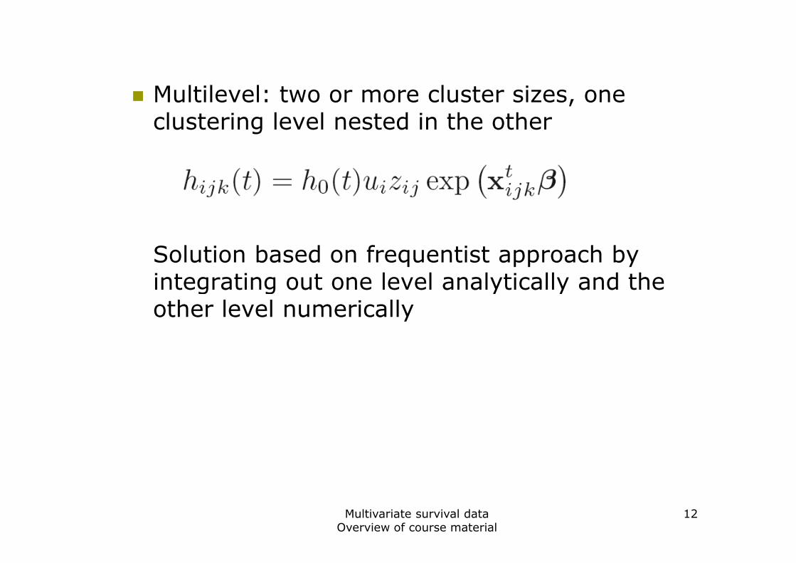
� Multilevel: two or more cluster sizes, one clustering level nested in the other
Solution based on frequentist approach by integrating out one level analytically and the integrating out one level analytically and the other level numerically
Multivariate survival data Overview of course material
12

Multivariate survival data Examples
13

Multivariate survival data types
� Criteria to categorise
� Cluster size: 1, 2, 3, 4, >4
� Hierarchy: 1 or 2 nesting levels
� Event ordering: none or ordered in space/time
Multivariate survival data Examples
14
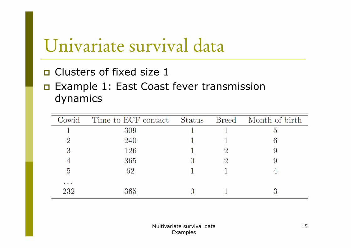
Univariate survival data
� Clusters of fixed size 1
� Example 1: East Coast fever transmission dynamics
Multivariate survival data Examples
15

Bivariate survival data
� Clusters of fixed size 2
� Example 2: diagnosis of fracture healing
Multivariate survival data Examples
16

� Example 3: Udder quarter reconstitution
17

Quadruples of correlated event times
� Cluster of fixed size 4
� Example 4: Correlated infection times in 4 udder quarters
Multivariate survival data Examples
18

Event times in clusters of varying sizeFew clusters of large size
� One level of clustering, but varying cluster size
� Example 5: Peri-operative breast cancer treatment
Multivariate survival data Examples
19

Event times in clusters of varying sizeMany small clusters
� One level of clustering, but varying cluster size
� Example 6: Breast conserving therapy for Ductal Carcinoma in Situ (DCIS)
Multivariate survival data Examples
20

Event times in clusters of varying sizeMany large clusters
� One level of clustering, but varying cluster size
� Example 7: Time to culling of heifer cows as a function of early somatic cell count
Multivariate survival data Examples
21

� Example 8: Time to first insemination of heifers as function of time-varying milk protein concentration
22

� Example 9: Time to first insemination of heifer cows as a function of initial milk protein concentration
23

� Example 10: Prognostic index evaluation in bladder cancer
24

Clustered event times with ordering
� Event times in a cluster have a certain ordering
� Example 11: Recurrent asthma attacks in children
Multivariate survival data Examples
25

Event times in 2 nested clustering levels
� Smaller clusters of event times are nested in a larger cluster
� Example 12: Infant mortality in Ethiopia
Multivariate survival data Examples
26

Modeling multivariate survival data.
The different approaches.
27

Overview
� Basic quantities/likelihood in survival
� The different approaches
� The marginal model
The fixed effects model� The fixed effects model
� The stratified model
� The copula model
� The frailty model
� Efficiency comparisons
Overview 28

Basic quantities in survival
� The probability density function of event time T
� The cumulative distribution function� The cumulative distribution function
� The survival function
Basic quantities/likelihood in survival 29

� The hazard function
� The cumulative hazard function
Basic quantities/likelihood in survival 30

Survival likelihood
�We consider the survival likelihood for right censored data ( ) assuming uninformative censoring
Basic quantities/likelihood in survival 31

Survival likelihood maximisation
�Likelihood maximisation leads to ML estimates, for instance, constant hazard
with likelihood and loglikelihoodwith likelihood and loglikelihood
�Equating first derivative to zero gives
Basic quantities/likelihood in survival 32

Survival likelihood maximisation: Example
�Time to diagnosis using US
� d=106,
Basic quantities/likelihood in survival 33

Survival likelihood maximisation: Example in R – explicit solution
�Time to diagnosis using US
library(survival)timetodiag <-read.table("c:\\docs\\bookfrailty\\data\\diag.csv",
Basic quantities/likelihood in survival 34
read.table("c:\\docs\\bookfrailty\\data\\diag.csv", header = T,sep=";")t1<-timetodiag$t1/30;t2<-timetodiag$t2/30c1<-timetodiag$c1;c2<-timetodiag$c2
#Explicit solution for lambdasumy<-sum(t1);d<-sum(c1);lambda1<-d/sumysumy;d;lambda1

Survival likelihood maximisation: Example in R – iterative solution
#likelihood maximisation
survlik<-function(p){d*log(p[1])+p[1]*sumy}
nlm(survlik,0.5)
$minimum [1] 162.3838
$estimate[1] 0.5874742
$gradient[1] 4.447998e-05
$code[1] 1
$iterations[1] 4
Basic quantities/likelihood in survival 35

Maximisation and Newton-Raphson
�Closed form solutions exist only in exceptional cases
�In most cases iterative procedures have to be used for maximisationbe used for maximisation
�Newton Raphson (NR) procedure finds a point for which
�Thus we can find the estimate that maximises the likelihood by using the NR procedure on the first derivative of the (log) likelihood
Basic quantities/likelihood in survival 36

Newton-Raphson procedure
� Aim: find point of function with
� We start with point
and use Taylor series expansion
� We only take first two terms and find
� We take the right hand side as new estimate and proceed iteratively
Basic quantities/likelihood in survival 37

Newton-Raphson procedure: Illustration
� Iterative procedure:
� Example graphically:
6
Basic quantities/likelihood in survival 38
x
f(x)
0.0 0.5 1.0 1.5 2.0
02
4

Newton-Raphson procedure Example� Estimating though NR:
40
Basic quantities/likelihood in survival 39
0.45 0.50 0.55 0.60 0.65 0.70
-20
020
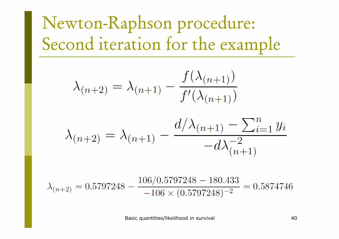
Newton-Raphson procedure: Second iteration for the example
Basic quantities/likelihood in survival 40

Variance estimate from likelihood
�An estimate of the variance of is given by the inverse of minus the second derivative
Basic quantities/likelihood in survival 41
evaluated at
�Thus we have

Variance from likelihood in R
�Minus the second derivative(s) of the log likelihood is obtained when using option ‘hessian=T’
Basic quantities/likelihood in survival 42
survlik<-function(p){-d*log(p[1])+p[1]*sumy}
results<-nlm(survlik,0.5,hessian=T)
1/results$hessian
[,1]
[1,] 0.003257014

Multidimensional NR procedure
�The NR procedure for one parameter
Basic quantities/likelihood in survival 43
can be extended to multidimensional version
the observed information matrix and
the score vector

Overview
� Basic quantities/likelihood in survival
� The different approaches
� The marginal model
The fixed effects model� The fixed effects model
� The stratified model
� The copula model
� The frailty model
� Efficiency comparisons
Overview 44

The marginal model
� The marginal model approach consists of two stages
� Stage 1: Fit the model without taking into account the clustering
Stage 2: Adjust for the clustering in the data� Stage 2: Adjust for the clustering in the data
The different approaches - the marginal model 45

Consistency of marginal model parameter estimates
� The ML estimate from the Independence Working Model (IWM)
is a consistent estimator for (Huster, 1989)
� More generally, the ML estimate ( and possibly baseline parameters) from the IWM is also a consistent estimator for
� Parameter refers to the wholewhole population
The different approaches - the marginal model 46

Adjusting the variance of IWM estimates
� The variance estimate based on the inverse of the information matrix of is an inconsistent
estimator of Var( )
� One possible solution: jackknife estimation � One possible solution: jackknife estimation
� General expression of jackknife estimator for iid data (Wu, 1986)
with N the number of observations and a the number of parameters
The different approaches - the marginal model 47

The grouped jackknife estimator
� For clustered observations: grouped jackknife estimator
with s the number of clusters
The different approaches - the marginal model 48
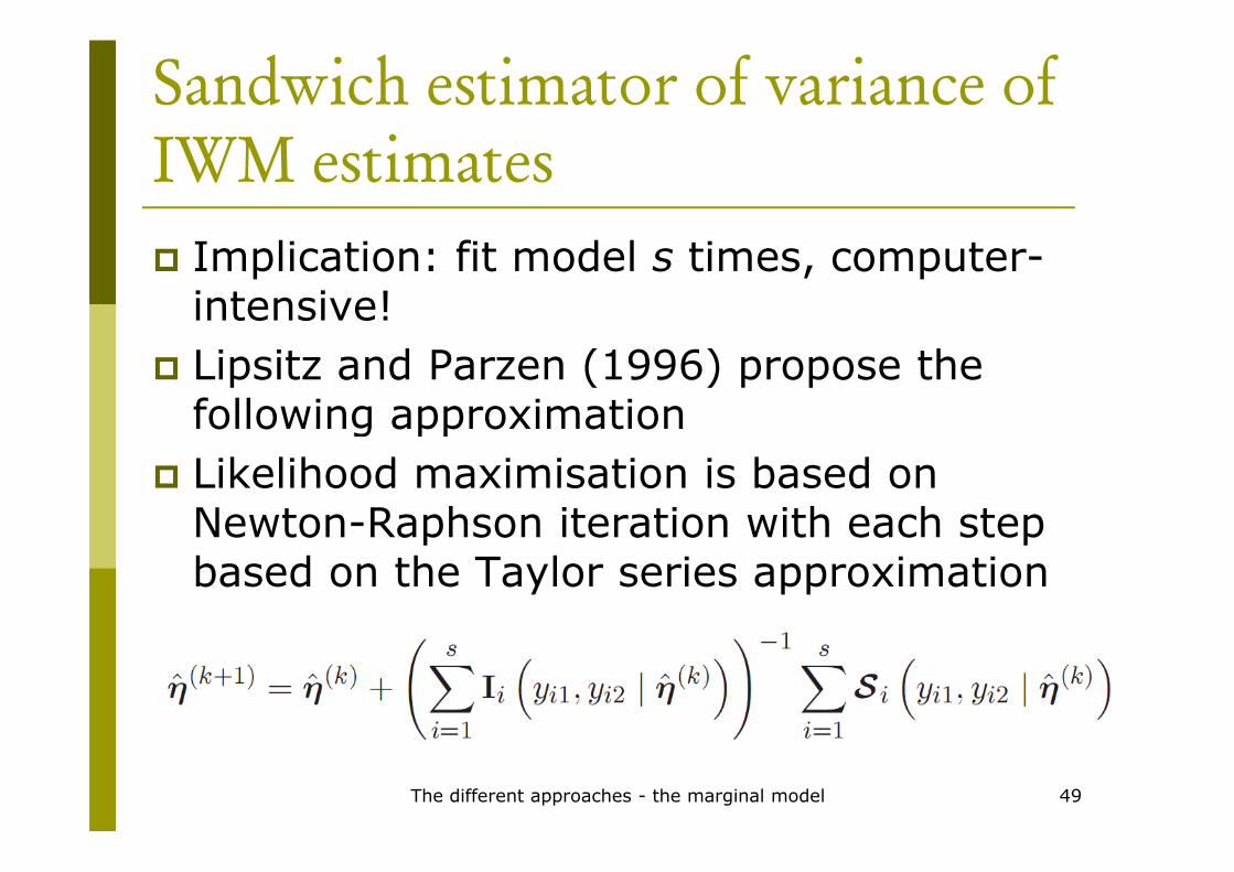
Sandwich estimator of variance of IWM estimates
� Implication: fit model s times, computer-intensive!
� Lipsitz and Parzen (1996) propose the following approximationfollowing approximation
� Likelihood maximisation is based on Newton-Raphson iteration with each step based on the Taylor series approximation
The different approaches - the marginal model 49

� A good starting value is , and the first Newton-Raphson iteration step is then
In this expression, however, we have� In this expression, however, we have
The different approaches - the marginal model 50

… and can thus be rewritten as
� Plugging this into the grouped jackknife:
The different approaches - the marginal model 51

� Further assume s>>a and always using the same information matrix, we obtain the robust variance estimator
with the information matrix and with the information matrix and the score vector
� This approximation corresponds to the sandwich estimator obtained by White (1982) starting from a different viewpoint.
The different approaches - the marginal model 52

Example marginal model with jackknife estimator
� Example 3: Blood-milk barrier reconstitution
� Estimates from IWM model with time-constant hazard rate assumption are given constant hazard rate assumption are given by
� Grouped jackknife = approximation
The different approaches - the marginal model 53

The jackknife estimator in R
� Reading the data
reconstitution<-read.table ("c://docs//presentationsfrailty//Rotterdam//data//reconstitution.csepv",header=T,sep=",")
#Create 5 column vectors, five different variables#Create 5 column vectors, five different variables
cowid<- reconstitution$cowid
timerec<-reconstitution$timerec
stat<- reconstitution$stat
trt<- reconstitution$trt
heifer<- reconstitution$heifer
The different approaches - the marginal model 54

� Fitting the unadjusted model
res.unadjust<-survreg(Surv(timerec,stat)~trt,dist="exponential",data=reconstitution)
b.unadjust<- -res.unadjust$coef[2]
stdb.unadjust<- sqrt(res.unadjust$var[2,2])
l.unadjust<-exp(-res.unadjust$coef[1])
The different approaches - the marginal model 55

� Obtaining the grouped jackknife estimator
dat<-data.frame(timerec=timerec,trt=trt,stat=stat,cowid=cowid)
res<-survreg(Surv(timerec,stat)~trt,data=dat,dist="exp")
init<-c(res$coeff[1],res$coeff[2])
ncows<-length(levels(as.factor(cowid)))
bdel<-matrix(NA,nrow=ncows,ncol=2)bdel<-matrix(NA,nrow=ncows,ncol=2)
for (i in 1:ncows){
temp<-reconstitution[reconstitution$cowid!=i,]
coeff<-survreg(Surv(timerec,stat)~trt, data=temp,dist="exponential")$coeff
bdel[i,1]<- -coeff[2];bdel[i,2]<-exp(-coeff[1])}
sqrt(0.98*sum((bdel[,1]-b.unadjust)^2))
The different approaches - the marginal model 56

� Obtaining the grouped 1-step jackknife estimator
bdel<-matrix(NA,nrow=ncows,ncol=2)
for (i in 1:ncows){
temp<-reconstitution[reconstitution$cowid!=i,]
coeff<-survreg(Surv(timerec,stat)~trt,data=temp, init=init,maxiter=1,dist="exponential")$coeff
bdel[i,1]<- -coeff[2]bdel[i,1]<- -coeff[2]
bdel[i,2]<-exp(-coeff[1])
}
sqrt(0.98*sum((bdel[,1]-b.unadjust)^2))
The different approaches - the marginal model 57

The jackknife estimator in R Problems
� The grouped jackknife estimator can be obtained right away by the ‘cluster’ command
� For Weibull, for instance, we have
res.adjust<-survreg(Surv(timerec,stat)~trt+cluster(cowid), res.adjust<-survreg(Surv(timerec,stat)~trt+cluster(cowid), data=reconstitution)
� For exponential, this does not seem to work …
The different approaches - the marginal model 58

Jackknife estimator-simulations
� In the example, the jackknife estimate of the variance is SMALLER than the unadjusted variance!!
� Is the jackknife estimate always smaller Is the jackknife estimate always smaller than estimate from unadjusted model, or does this depend on the data?
� Generate data from the frailty model of time to reconstitution data with
The different approaches - the marginal model 59

� We generate 2000 datasets, each of 100 pairs of two subjects for the settings
1. Matched clusters, no censoring
2. 20% of clusters 2 treated or untreated subjects, no censoring
3. Matched clusters, 20% censoring3. Matched clusters, 20% censoring
Matched clusters: the two animals sharing the clusters have different covariate levels
The different approaches - the marginal model 60

� Simulation results
The different approaches - the marginal model 61

The fixed effects model
� The fixed effects model is given by
with the fixed effect for cluster i,with the fixed effect for cluster i,
� Assume for simplicity and
with
The different approaches - the fixed effects model 62

The fixed effects model: ML solution
� General survival likelihood expression
� For fixed effects model with constant hazard
The different approaches - the fixed effects model 63

Fixed effects and loglinear model
� Software often uses loglinear model
with, for ,
Gumbel
� Comparison can be based on S(t)
The different approaches - the fixed effects model 64

Survival function loglinear model (1)
� We look for
� General rule� General rule
� Applied to
The different approaches - the fixed effects model 65

Equivalence fixed effects model and loglinear model
� Therefore, we have for loglinear model
vs
The different approaches - the fixed effects model 66

The delta method - general
� Original parameters
� Interest in univariate cont. function
� Use one term Taylor expansion of
with
The different approaches - the fixed effects model 67

The delta method - specific
� Interest in univariate cont. function
� The one term Taylor expansion of
with
The different approaches - the fixed effects model 68

� Treatment effect for reconstitution data using R-function survreg (loglin. model):
the effect of the drug
Example: within cluster covariate
res.fixed.trt<-survreg(Surv(timerec,stat)~
The different approaches - the fixed effects model 69
res.fixed.trt<-survreg(Surv(timerec,stat)~ as.factor(cowid)+as.factor(trt), dist="exponential",data=reconstitution)summary(res.fixed.trt)
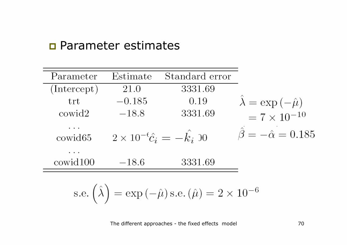
� Parameter estimates
The different approaches - the fixed effects model 70

� Parameter interpretation
� corresponds to constant hazard of untreated udder quarter of cow 1
� corresponds to constant hazard of untreated udder quarter of cow i
� Cowid65 ≈ 0� Cowid65 ≈ 0
� Cowid100 exp(-21+18.8)=0.11
� Treatment effect: HR=exp(0.185)=1.203 with 95% CI [0.83;1.75]
The different approaches - the fixed effects model 71

� Heifer effect for reconstitution data
introducing heifer first in the model
Example: between cluster covariate
Hazard ratio impossibly high
The different approaches - the fixed effects model 72

� Heifer effect for reconstitution data
introducing cowids first in the model
Hazard ratio equal to 1
The different approaches - the fixed effects model 73

� Heifer effect for reconstitution data
� Two estimates for heifer effect, which one (if any) is correct? Write down incidence matrix for intercept, cowid and heifer for 6 cows, with first 3 cows being heifers
The different approaches - the fixed effects model 74

Intercept ci2 ci3 ci4 ci5 ci6 heifer parityC1 C2 C3 C4 C5 C6 C7 C8
� Incidence matrix heifer – cowid
The different approaches - the fixed effects model 75
C7=C1-C4-C5-C6 COMPLETE CONFOUNDING

Intercept ci2 ci3 ci4 ci5 ci6 heifer parityC1 C2 C3 C4 C5 C6 C7 C8
� Incidence matrix heifer – cowid
The different approaches - the fixed effects model 76
C8=C1+C4+C5+3C6 COMPLETE CONFOUNDING

The stratified model
� The stratified model is given by
� Maximisation of partial likelihood,� Maximisation of partial likelihood,
with the risk set for cluster i
The different approaches - the stratified model 77

Example for bivariate data
� Consider the case of bivariate data, e.g. the reconstitution data
� Write down a simplified version of the general expression
� When does a cluster contribute to the likelihood?
The different approaches - the stratified model 78

� The partial likelihood for reconstitution data
� Estimates
The different approaches - the stratified model 79

The stratified model in R
� Use the coxph function for time to reconstution data > res.strat.trt<-coxph(Surv(timerec,stat)~as.factor(trt) +strata(cowid),data=reconstitution)> summary(res.strat.trt)
coef exp(coef) se(coef) z pas.factor(trt)1 0.131 1.14 0.209 0.625 0.53
exp(coef) exp(-coef) lower .95 upper .95as.factor(trt)1 1.14 0.878 0.757 1.72
Likelihood ratio test= 0.39 on 1 df, p=0.531Wald test = 0.39 on 1 df, p=0.532Score (logrank) test = 0.39 on 1 df, p=0.532
The different approaches - the stratified model 80

The copula model
� If all clusters have the same size, another useful approach is the copula model
� We consider bivariate data in which the first (second) subject in each cluster has first (second) subject in each cluster has the same covariate information, and the covariate information differs between the two subjects in the same cluster
� Time to diagnosis of
being healed
The different approaches - the copula model 81

The two stage approach
� A copula model is often fitted using a two-stage model:
� First specify the population (marginal) survival functions for the first (second) subject in a cluster and obtain estimates for them.cluster and obtain estimates for them.
� We then generate the joint survival function by linking the population survival functions through the survival copula function (Frees et al., 1996).
The different approaches - the copula model 82

Example of copula model
� Time to diagnosis of being healed
The different approaches - the copula model 83

Bivariate copula model likelihood
� Four different possible contributions of a cluster
� Estimated population survival functions are inserted, only copula parameters unknown
The different approaches - the copula model 84

The Clayton copula
� The Clayton copula (Clayton, 1978) is
� The Clayton copula corresponds to the � The Clayton copula corresponds to the family of Archimedean copulas, i.e.,
with in the Clayton copula case
The different approaches - the copula model 85

Clayton copula likelihood for parametric marginals
� Two censored observations
� Observation j censored
� No obervations censored
86

Example Clayton copula
� For diagnosis of being healed data, first fit separate models for RX and US technique
� For instance, separate parametric models
The different approaches - the copula model 87

� Estimates for marginal models are
� Based on these estimates we obtain
which can be inserted in the likelihood expression which is then maximised for
The different approaches - the copula model 88

� For parametric marginal models, the likelihood can also be maximised simul-taneously for all parameters leading to
� Thus, for small sample sizes, the two-stage approach can differ substantially from the one-stage approach
The different approaches - the copula model 89

� Alternatives can be used for marginal models
� Nonparametric models
� Semiparametric models
leading to
The different approaches - the copula model 90

Clayton copula in Rtimetodiag <- read.table("c:\\docs\\bookfrailty\\data\\diag.csv",
header = T,sep=";")
t1<-timetodiag$t1/30;t2<-timetodiag$t2/30
c1<-timetodiag$c1;c2<-timetodiag$c2
surv1<-survreg(Surv(t1,c1)~1); surv2<-survreg(Surv(t2,c2)~1)surv1<-survreg(Surv(t1,c1)~1); surv2<-survreg(Surv(t2,c2)~1)
l1<- exp(-surv1$coeff/surv1$scale);r1<-(1/surv1$scale)
l2<-exp(-surv2$coeff/surv2$scale);r2<-(1/surv2$scale)
s1<-exp(-l1*t1^(r1));f1<-s1*r1*l1*t1^(r1-1)
s2<-exp(-l2*t2^(r2));f2<-s2*r2*l2*t2^(r2-1)
The different approaches - the copula model 91

� R-function
loglikcon.gamma.twostage<-function(theta){
P<-s1^(-theta)+ s2^(-theta)-1
loglik<- -(1-c1)*(1-c2)*(1/theta)*log(P)
+c1*(1-c2)*(-(1+1/theta)*log(P)-(theta+1)*log(s1)+log(f1))
+c2*(1-c1)*(-(1+1/theta)*log(P)-(theta+1)*log(s2)+log(f2))
+c1*c2*(log(1+theta)-(2+1/theta)*log(P)-(theta+1)*log(s1)+log(f1)-(theta+1)*log(s2)+log(f2))
-sum(loglik)-sum(loglik)
}
nlm(loglikcon.gamma.twostage,c(0.5))
The different approaches - the copula model 92

� Results of R-function
> nlm(loglikcon.gamma.twostage,c(0.5))
$minimum
[1] 233.0512
$estimate
[1] 0.9659607
$gradient$gradient
[1] 4.197886e-05
$code
[1] 1
$iterations
[1] 4
The different approaches - the copula model 93
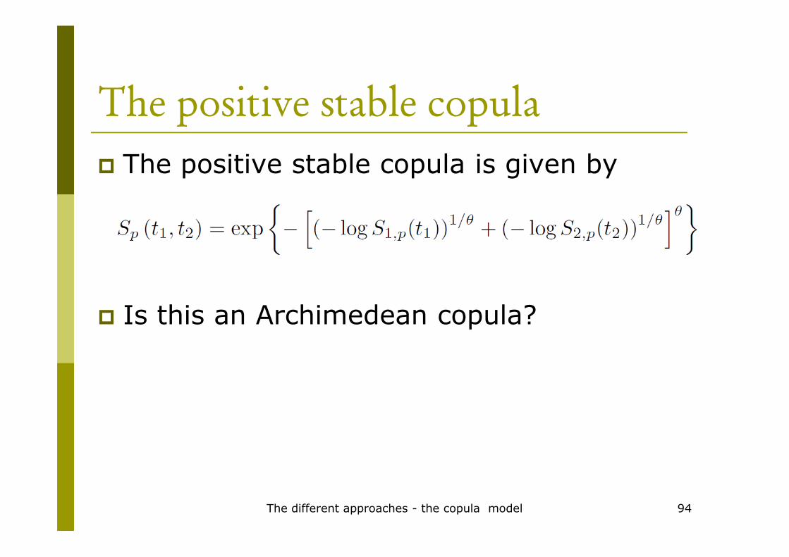
The positive stable copula
� The positive stable copula is given by
� Is this an Archimedean copula?
The different approaches - the copula model 94

The positive stable copula
� The positive stable copula is given by
� Is this an Archimedean copula?� Is this an Archimedean copula?
� Yes, it is, take
The different approaches - the copula model 95

The positive stable copula and likelihood contributions
� The positive stable copula is given by
� Write down the likelihood assuming a semiparametric model for the population survival functions
The different approaches - the copula model 96

� The positive stable copula is given by
� Write down the likelihood assuming a nonparametric model for the population survival functions survival functions
� No events:
The different approaches - the copula model 97

� Likelihood contributions
� No events
� One event
� Two events
The different approaches - the copula model 98

The frailty model
� The ‘shared’ frailty model is given by
with the frailtywith the frailty
� An alternative formulation is given by
with
The different approaches - the frailty model 99

The gamma frailty model
� Gamma frailty distribution is easiest choice
with and
The different approaches - the frailty model 100

Marginal likelihood for the gamma frailty model
� Start from conditional (on frailty) likelihood
with containing the baseline hazard
parameters, e.g., for Weibull
The different approaches - the frailty model 101

Marginal likelihood: integrating out the frailties …
� Integrate out frailties using distribution
with
The different approaches - the frailty model 102

Closed form expression for marginal likelihood
� Integration leads to
The different approaches - the frailty model 103

Maximisation of marginal likelihood leads to estimates
� Marginal likelihood no longer contains frailties. By maximisation estimates of
are obtained
� Furthermore, the asymptotic variance-� Furthermore, the asymptotic variance-covariance matrix can be obtained as the inverse of the observed information matrix
with the Hessian
matrix with entries
The different approaches - the frailty model 104

Efficiency comparisons in the reconstitution data example
� Estimates (se) for reconstitution data
The different approaches – efficiency comparisons 105

Efficiency comparisons-theory
� For parametric model with constant hazard, we can obtain the expected information for (Wild, 1983)
� Due to asymptotic independence of parameters, the asymptotic variance for is given by
The different approaches – efficiency comparisons 106

� Unadjusted model
� Fixed effects model
Frailty model� Frailty model
The different approaches – efficiency comparisons 107

Efficiency comparisons-simulations
� Generate data from the frailty model with
� We generate 2000 datasets, each of 100 � We generate 2000 datasets, each of 100 pairs of two subjects for the settings
1. Matched clusters, no censoring
2. 20% of clusters 2 treated or untreated subjects, no censoring
3. Matched clusters, 20% censoring
The different approaches – efficiency comparisons 108

� Simulation results
The different approaches – efficiency comparisons 109

Semantics and History of the term frailty
110

Semantics of term frailty
� Medical field: gerontology
� Frail people higher morbidity/mortality risk
� Determine frailty of a person (e.g. Get-up and Go test)
Frailty: fixed effect, time varying, surrogate� Frailty: fixed effect, time varying, surrogate
� Modelling: statistics
� Frailty often at higher aggregation level (e.g. hospital in multicenter clinical trial)
� Frailty: random effect, time constant, estimable
Frailty semantics 111

History of term frailty - Beard
� Introduced by Beard (1959) in univariate setting to improve population mortality modelling by allowing heterogeneity
� Beard (1959) starts from Makeham’s law (1868)
with the constant hazard and with
the hazard increases with time
� Longevity factor is added to model
Frailty semantics 112

� Beard’s model
� Population survival function
� Population hazard function Hazard at time t forsubject with frailty u
Frailty semantics 113
Survival at time t forsubject with frailty u
subject with frailty u

� With one parameter gamma distribution as frailty distribution, we obtain a Perk’s logistic curve
Frailty semantics 114
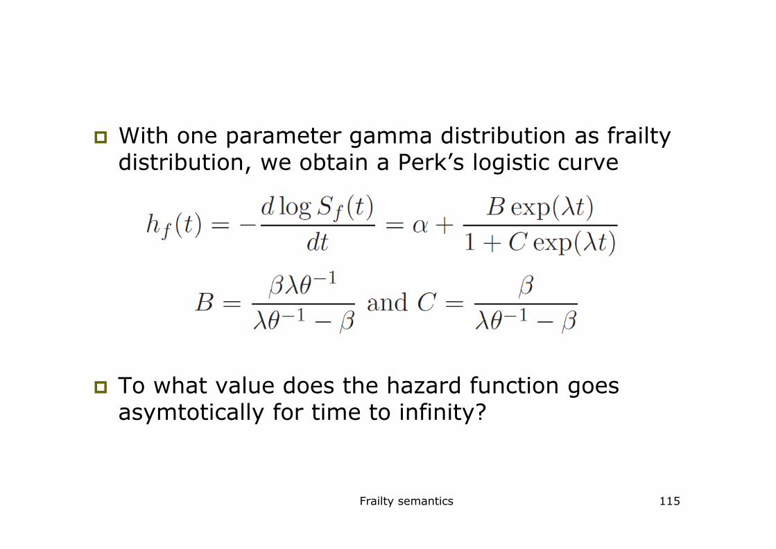
� With one parameter gamma distribution as frailty distribution, we obtain a Perk’s logistic curve
� To what value does the hazard function goes asymtotically for time to infinity?
Frailty semantics 115

� The hazard function of Perk’s logistic curve starts at and goes asymptotically to
� Example:
Frailty semantics 116

� Term frailty first introduced by Vaupel (1979) in univariate setting to obtain individual mortality curve from population mortality curve
History of term frailty - Vaupel
Frailty semantics 117
mortality curve
� For the case of no covariates

� Vaupel assumed gamma frailties and thus
Frailty semantics 118
Conditional mean decreases with time, Individual hazard increases relatively with time

� From hazard to conditional probability
Frailty semantics 119

� Example Swedish population two centuries
Frailty semantics 120

� Example Swedish population two centuries
Frailty semantics 121

� Vaupel and Yashin (1985) studied heterogeneity due to two subpopulations
� Population 1:
� Population 2:
Frailty – two subpopulations
Frailty semantics 122

� Smokers:high and low recidivism rate
� Is the population hazard constant, decreasing or increasing over time?
Frailty semantics 123
decreasing or increasing over time?
� Calculate the population hazard at time 0 and at 20 years.

� Smokers:high and low recidivism rate
� The population hazard
� At time 0:
At 20 years:
Frailty semantics 124
� At 20 years:

� Smokers:high and low recidivism rate: pictures
Frailty semantics 125

� Reliability engineering
Frailty semantics 126

� Two hazards increasing at different rates
Frailty semantics 127

� Two parallel hazards (at log scale)
Frailty semantics 128

Basics of parametric gamma frailty model
129

Overview
� The gamma (frailty) density
� The marginal likelihood for the parametric gamma frailty model
� An example: time to first insemination with � An example: time to first insemination with heifer as covariate
� Laplace transform
� From the joint survival function to the marginal likelihood
� Functions at the population level
� An example: udder quarter infection data
Overview 130

The gamma frailty density
� Two-parameter gamma density
� One-parameter gamma density:
The gamma frailty density 131

� One-parameter gamma density: pictures
The gamma frailty density 132

� Shared gamma frailty model (a conditional hazards model)
The marginal likelihood for the parametric gamma frailty model
� The conditional likelihood for cluster i is
The marginal likelihood for the parametric gamma frailty model
133
with a random sample from one-parameter gamma density

� The marginal likelihood for cluster i is, with and ,
which has the following explicit solution
The marginal likelihood for the parametric gamma frailty model
134

� The marginal loglikelihood is
where
� ML estimates for the components of can be found by maximising this loglikelihood.
� The estimated variance-covariance matrix is obtained as the inverse of the observed information matrix evaluated at ,
The marginal likelihood for the parametric gamma frailty model
135

� See Example 9
� The hazard for cow j from herd i is
An example: time to first insem-ination with heifer as covariate
with the heifer covariate ( for multiparous, for heifer), the heifer effect and
� Assume Weibull, then
i.e., given the value of the event times follow a Weibull distribution with parameters and
An example: time to first insemination with heifer as covariate
136
for heifer), the heifer effect and the frailty term for herd i

� Maximising the marginal loglikelihood (with time in months – for convergence reasons) we obtain
� For herd with the hazard ratio is exp(-0.153) = 0.858. The 95% CI is [0.820,0.897], i.e., the hazard of first insemination for heifers is significantly lower.
An example: time to first insemination with heifer as covariate
137

� Relation between months and days
(the cumulative hazard ratio at any time is required to be the same)
An example: time to first insemination with heifer as covariate
138

� Hazard functions for time to first insemination
An example: time to first insemination with heifer as covariate
139

� Median time to event for herd i in heifers, resp. multiparous cows ( ,resp. ): ( ,resp. ).
An example: time to first insemination with heifer as covariate
140

� Median time to first insemination
An example: time to first insemination with heifer as covariate
141

� First read in time to first insemination data
#Read data
insemfix<-read.table("c://docs//presentationsfrailty//Rotterdam//data
Maximising marginal likelihood in R
read.table("c://docs//presentationsfrailty//Rotterdam//data//insemination.datc", header=T,sep=",")
#Create four column vectors, four different variables
herd<-insemfix$herdnr;timeto<-(insemfix$end*12/365.25)
stat<-insemfix$score;heifer<-insemfix$par2
#Derive some values
n<-length(levels(as.factor(herd)))
di<-aggregate(stat,by=list(herd),FUN=sum)[,2];r<-sum(di)
Maximising marginal likelihood in R 142

� Define loglikelihood function for transformed parameters
#Observable likelihood weibull with transformed variables
#l=exp(p[1]), theta=exp(p[2]), beta=p[3], rho=exp(p[4])
#r=No events,di=number of events by herd
likelihood.weibul<-function(p){
cumhaz<-exp(heifer*p[3])*(timeto^(exp(p[4])))*exp(p[1])
cumhaz<-aggregate(cumhaz,by=list(herd),FUN=sum)[,2]cumhaz<-aggregate(cumhaz,by=list(herd),FUN=sum)[,2]
lnhaz<-stat*(heifer*p[3]+log((exp(p[4])*timeto^(exp(p[4])-1))*exp(p[1])))
lnhaz<-aggregate(lnhaz,by=list(herd),FUN=sum)[,2]
lik<-r*log(exp(p[2]))-sum((di+1/exp(p[2]))*log(1+cumhaz*exp(p[2])))+sum(lnhaz)+sum(sapply(di,function(x) ifelse(x==0,0,log(prod(x+1/exp(p[2])-seq(1,x))))))
-lik}
Maximising marginal likelihood in R143

� Maximise the function for the transformed parameters and return parameter estimates
res<-nlm(likelihood.weibul,c(log(0.174),log(0.39),-0.15,log(1.76)))
lambda<-exp(res$estimate[1])
theta<-exp(res$estimate[2])
beta<-res$estimate[3]beta<-res$estimate[3]
rho<-exp(res$estimate[4])
Maximising marginal likelihood in R144
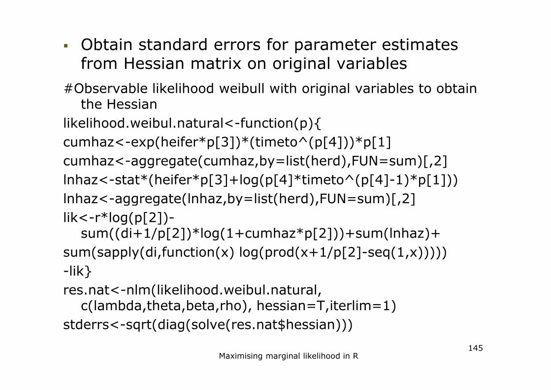
� Obtain standard errors for parameter estimates from Hessian matrix on original variables
#Observable likelihood weibull with original variables to obtain the Hessian
likelihood.weibul.natural<-function(p){
cumhaz<-exp(heifer*p[3])*(timeto^(p[4]))*p[1]
cumhaz<-aggregate(cumhaz,by=list(herd),FUN=sum)[,2]
lnhaz<-stat*(heifer*p[3]+log(p[4]*timeto^(p[4]-1)*p[1]))
lnhaz<-aggregate(lnhaz,by=list(herd),FUN=sum)[,2]lnhaz<-aggregate(lnhaz,by=list(herd),FUN=sum)[,2]
lik<-r*log(p[2])-sum((di+1/p[2])*log(1+cumhaz*p[2]))+sum(lnhaz)+
sum(sapply(di,function(x) log(prod(x+1/p[2]-seq(1,x)))))
-lik}
res.nat<-nlm(likelihood.weibul.natural, c(lambda,theta,beta,rho), hessian=T,iterlim=1)
stderrs<-sqrt(diag(solve(res.nat$hessian)))
Maximising marginal likelihood in R145

� Characteristic function
� Moment generating function
Laplace transform
� Laplace transform for positive r.v.
Laplace transform 146

� Generate nth moment
� Use nth derivative of Laplace transform
� Evaluate at s=0
� The Laplace transform for the one-parameter gamma density is
Laplace transform147

� Joint survival function in conditional model
� Use as notation
From the joint survival and density functions to the marginal likelihood
� For cluster of size n with covariates
From the joint survival and density functions to the marginal likelihood
148

� For cluster of size n with covariates the joint density is
From the joint survival and density functions to the marginal likelihood
149

� Applied to Laplace transform of gamma frailty we obtain
From the joint survival and density functions to the marginal likelihood
150
=

� Note. Same as the , but now from more general Laplace point of view.
From the joint survival and density functions to the marginal likelihood
151

� Population survival function (integrate out the frailty from the conditional survival function)
� Population density function
Functions at the population level
� Population density function
� Population hazard function
Functions at the population level 152

� Ratio of population and conditional hazard
� Applied to the gamma frailty we have
Functions at the population level 153

� Ratio of population and conditional hazard for the gamma frailty
Functions at the population level 154

� Population hazard ratio for a binary (0-1) covariate
� Applied to the gamma frailty we have
Functions at the population level 155

� Population hazard ratio for the gamma frailty
Functions at the population level 156

� In general we have
� Applied to the gamma frailty we have
Updating (no covariates, gamma frailty)
� Applied to the gamma frailty we have
Updating (no covariates, gamma frailty)
157

with conditionial mean
and conditional variance
Updating (no covariates, gamma frailty)
158

� Conditionial variance of U
Updating (no covariates, gamma frailty)
159

� See Example 4
� Binary covariate: heifer/multiparous ( is the heifer effect)
Weibull baseline hazard
Gamma frailty density
Maximising the marginal loglikelihood we obtain
An example: udder quarter infection data
� Maximising the marginal loglikelihood we obtain
An example: udder quarter infection data 160

� Conditional and population hazard ratio functions
Updating (no covariates, gamma frailty)
161

� Hazard ratio multiparous cow versus heifer
1.1
1.2
1.3
1.4
1.5
1.6
Haz
ard
ratio
Updating (no covariates, gamma frailty)
162
0 1 2 3 4Time (year quarters)
1.0
1.1

� Mean and variance of conditional frailty density
Updating (no covariates, gamma frailty)
163

The parametric gamma frailty model: variations on
the theme
Overview
� A piecewise constant baseline hazard
� Recurrent events
164

A piecewise constant baseline hazard
� See Example 7
� Event time: time to culling
Covariate: logarithm of somatic cell count (SCC)
The model � The model
� The MLE are given by
A piecewise constant baseline hazard 165

� LR test for constant baseline hazard versus piecewise constant baseline hazard
versus
The p-value (using a -distribution with 2 degrees of freedom) is smaller than 0.00001
A piecewise constant baseline hazard 166

� First read in time to culling data
#Read data
culling<-read.table('c://culling.datc',header=T,sep=",")
culltime<-culling$timetocul*12/365.25
logSCC<-culling$logSCC
Time to culling: piecewise constant hazard frailty model in R
logSCC<-culling$logSCC
herd<-as.factor(culling$herdnr)
status<-culling$status
endp1<-70*12/365.25;endp2<-300*12/365.25
n<-length(levels(as.factor(herd)))
di<-aggregate(status,by=list(herd),FUN=sum)[,2]
r<-sum(di))
A piecewise constant baseline hazard 167

� Fit model with linear effect of log(SCC), constant hazard
#parametric exponential covariate lnscc1
likelihood.exp<-function(p){
cumhaz<-exp(logSCC*p[1])*exp(p[3])*culltime
cumhaz<-aggregate(cumhaz,by=list(herd),FUN=sum)[,2]
lnhaz<-status* (logSCC*p[1]+log(exp(p[3])))
lnhaz<-aggregate(lnhaz,by=list(herd),FUN=sum)[,2]
lik<-r*log(exp(p[2]))-sum((di+1/exp(p[2])) lik<-r*log(exp(p[2]))-sum((di+1/exp(p[2])) *log(1+cumhaz*exp(p[2]))) +sum(lnhaz)-n*log(gamma(1/exp(p[2]))) +sum(log(gamma(di+1/exp(p[2]))))
-lik}
initial<-c(0,log(0.2),log(0.01))
t<-nlm(likelihood.exp,initial,print.level=2)
beta<-t$estimate[1];theta<-exp(t$estimate[2])
lambda<-exp(t$estimate[3]);likelihood.linear<-t$minimumA piecewise constant baseline hazard 168

� Results model with linear effect of log(SCC), constant hazard
beta<-t$estimate[1]
theta<-exp(t$estimate[2])
lambda<-exp(t$estimate[3])
likelihood.linear<-t$minimum
> beta> beta
[1] 0.08813477
> theta
[1] 0.06230903
> lambda
[1] 0.01606552
> likelihood.linear
[1] 15079.36
A piecewise constant baseline hazard 169

� Fit model with linear effect of log(SCC); piecewise constant hazard
likelihood.piecexp<-function(p){
cumhaz<-exp(logSCC*p[1])*exp(p[3])*pmin(culltime,endp1)
cumhaz<-cumhaz+exp(logSCC*p[1]) *exp(p[4])*pmax(0,pmin(endp2-endp1,culltime-endp1))
cumhaz<-cumhaz+exp(logSCC*p[1])*exp(p[5]) *pmax(0,culltime-endp2)
cumhaz<-aggregate(cumhaz,by=list(herd),FUN=sum)[,2]
lnhaz<-status*(logSCC*p[1]+log(as.numeric(culltime<endp1)* lnhaz<-status*(logSCC*p[1]+log(as.numeric(culltime<endp1)* exp(p[3])+as.numeric(endp1<=culltime) *as.numeric(culltime<endp2)*exp(p[4]) +as.numeric(culltime>=endp2)*exp(p[5])))
lnhaz<-aggregate(lnhaz,by=list(herd),FUN=sum)[,2]
lik<-r*log(exp(p[2]))-sum((di+1/exp(p[2]))*log(1+cumhaz*exp(p[2])))+ sum(lnhaz)-n*log(gamma(1/exp(p[2]))) +sum(log(gamma(di+1/exp(p[2]))))
-lik}
A piecewise constant baseline hazard 170

initial<-c(0,log(0.2),log(0.01),log(0.01),log(0.01))
t<-nlm(likelihood.piecexp,initial,print.level=2)
beta<-t$estimate[1];theta<-exp(t$estimate[2])
lambda1<-exp(t$estimate[3]);lambda2<-exp(t$estimate[4])
lambda3<-exp(t$estimate[5])
likelihood.piecewise<-t$minimum
> beta
[1] 0.08831314
> theta
[1] 0.1440544[1] 0.1440544
> lambda1
[1] 0.006735632
> lambda2
[1] 0.01151625
> lambda3
[1] 0.09857648
> likelihood.piecewise
[1] 13562.13
A piecewise constant baseline hazard 171

� Comparing constant and piecewise constant hazard ffunction models
> LR<-2*(-likelihood.piecewise+likelihood.linear)
> 1-pchisq(LR,2)
[1] 0
A piecewise constant baseline hazard 172

Recurrent events
� See Example 11
� Time to asthma attack is the event time
Covariate: placebo versus drug
� Patient i has ni at risk periods
which can be represented in a graphical way (first two patients)
Recurrent events 173

� Different timescales can be considered
� Calendar time
� Gap time
Recurrent events 174

� We give four conditional hazard models and we use the marginal likelihood to estimate the model parameters
For all four models the marginal likelihood that needs to be maximised is
where
For each of the four models we need to specify the precise meaning of and
Recurrent events 175
drug effect
heterogeneity between patients
Weibull baseline hazard

� Calendar time model
Weibull baseline hazard
Recurrent events 176

� Gap time model. Information used is
Weibull baseline hazard
Recurrent events 177

� Gap time model with hazard for first event different and constant
� Combining gap and calendar time
Recurrent events 178

� Overview of ML estimates for the four models
Recurrent events 179

� Graphical representation of the results
Recurrent events 180

� First read in asthma data
#Read data
w <-read.table("c:/docs/bookfrailty/data/asthma.dat",head=T)
di<-aggregate(w$st.w,by=list(w$id.w),FUN=sum)[,2]
Recurrent asthma attacks: Parametric frailty models in R
r<-sum(di);n<-length(di)
trt<-aggregate(w$trt.w,by=list(w$id.w),FUN=min)[,2]
begin<-12*w$start.w/365.25
end<-12*w$stop.w/365.25
ptno<-w$id.w;status<-w$st.w
gap<-end-begin;fevent<-w$fevent
Recurrent events 181
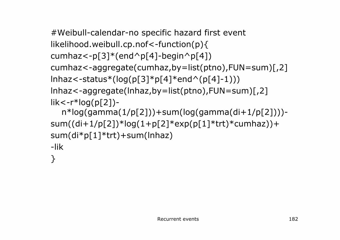
#Weibull-calendar-no specific hazard first event
likelihood.weibull.cp.nof<-function(p){
cumhaz<-p[3]*(end^p[4]-begin^p[4])
cumhaz<-aggregate(cumhaz,by=list(ptno),FUN=sum)[,2]
lnhaz<-status*(log(p[3]*p[4]*end^(p[4]-1)))
lnhaz<-aggregate(lnhaz,by=list(ptno),FUN=sum)[,2]
lik<-r*log(p[2])-n*log(gamma(1/p[2]))+sum(log(gamma(di+1/p[2])))-
sum((di+1/p[2])*log(1+p[2]*exp(p[1]*trt)*cumhaz))+sum((di+1/p[2])*log(1+p[2]*exp(p[1]*trt)*cumhaz))+
sum(di*p[1]*trt)+sum(lnhaz)
-lik
}
Recurrent events 182

#Weibull-gap-no specific hazardfirst event
likelihood.weibull.gap.nof<-function(p){
cumhaz<-p[3]*((end-begin)^p[4])
cumhaz<-aggregate(cumhaz,by=list(ptno),FUN=sum)[,2]
lnhaz<-status*(log(p[3]*p[4]*(end-begin)^(p[4]-1)))
lnhaz<-aggregate(lnhaz,by=list(ptno),FUN=sum)[,2]
lik<-r*log(p[2])-n*log(gamma(1/p[2]))+sum(log(gamma(di+1/p[2])))-
sum((di+1/p[2])*log(1+p[2]*exp(p[1]*trt)*cumhaz))+sum((di+1/p[2])*log(1+p[2]*exp(p[1]*trt)*cumhaz))+
sum(di*p[1]*trt)+sum(lnhaz)
-lik
}
Recurrent events 183

#Weibull-gap- first event exponential
likelihood.weibull.gap.fev.exp<-function(p){
cumhaz<- p[3]*(end-begin)*fevent+p[4]*((end-begin)^p[5])*(1-fevent)
cumhaz<-aggregate(cumhaz,by=list(ptno),FUN=sum)[,2]
lnhaz<-status*(log(p[3])*fevent+ log(p[4]*p[5]*(end-begin)^(p[5]-1))*(1-fevent))
lnhaz<-aggregate(lnhaz,by=list(ptno),FUN=sum)[,2]
lik<-r*log(p[2])-lik<-r*log(p[2])-n*log(gamma(1/p[2]))+sum(log(gamma(di+1/p[2])))-
sum((di+1/p[2])*log(1+p[2]*exp(p[1]*trt)*cumhaz))+
sum(di*p[1]*trt)+sum(lnhaz)
-lik
}
Recurrent events 184

#Weibull-gap-calendar-nofirstevent
likelihood.weibull.all<-function(p){
cumhaz<-p[3]*(end^p[4]-begin^p[4])+ (p[5]*((end-begin)^p[6])*as.numeric(begin!=0))
cumhaz<-aggregate(cumhaz,by=list(ptno),FUN=sum)[,2]
lnhaz<-status*( log( (p[3]*p[4]*end^(p[4]-1)) + as.numeric(begin!=0) * (p[5]*p[6]*(end-begin)^(p[6]-1))))
lnhaz<-aggregate(lnhaz,by=list(ptno),FUN=sum)[,2]lnhaz<-aggregate(lnhaz,by=list(ptno),FUN=sum)[,2]
lik<-r*log(p[2])-n*log(gamma(1/p[2]))+sum(log(gamma(di+1/p[2])))-
sum((di+1/p[2])*log(1+p[2]*exp(p[1]*trt)*cumhaz))+
sum(di*p[1]*trt)+sum(lnhaz)
-lik
}
Recurrent events 185

Dependence measures
186

Overview
� Setting, for i=1, …,s
binary data:
covariate information:
� Kendall’s : an overall measure of dependence
� The cross ratio function: a local measure of dependence
� Other local dependence measures
� An example: the gamma frailty for
Overview 187

Kendall’s τ: an overall measure of dependence
�
�
�
Kendall’s τ 188

� Express p in terms of joint survival and joint density function
using
Kendall’s τ 189

�
� Use
to obtain
Kendall’s τ 190

� Applied to the gamma frailty we obtain
Kendall’s τ 191

The cross ratio function: a local measure of dependence
�
See Example 3: time to blood-milk barrier � See Example 3: time to blood-milk barrier reconstitution
Positive experience: reconstitution at time t2For positively correlated data, we assume that hazard in numerator > hazard in denominator
The cross ratio function 192
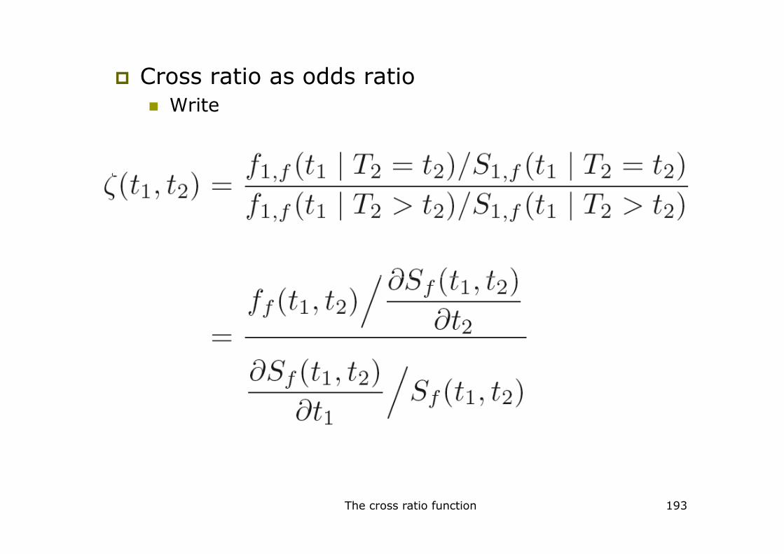
� Cross ratio as odds ratio
� Write
The cross ratio function 193
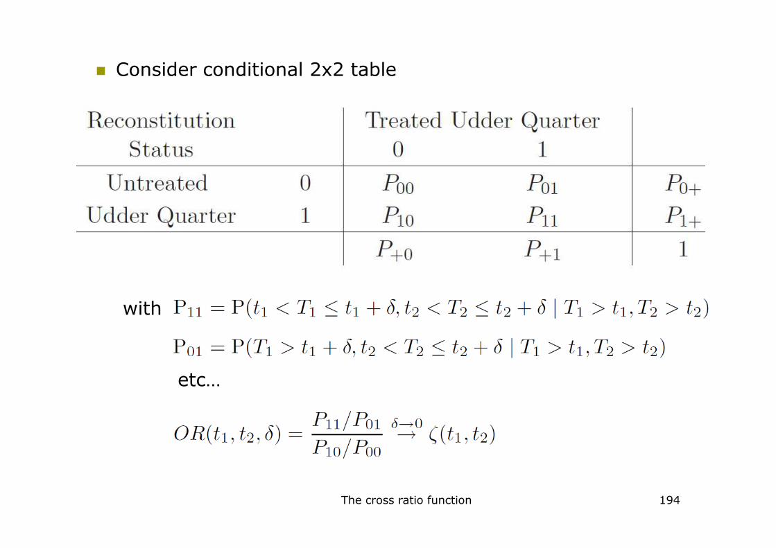
� Consider conditional 2x2 table
with
The cross ratio function 194
etc…
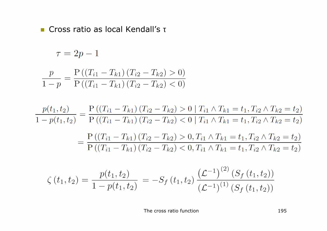
� Cross ratio as local Kendall’s τ
The cross ratio function 195

Other local dependence measures
�
�
Other local dependence measures 196

An example: the gamma frailty for θ=2/3
�
Other local dependence measures 197
see figures next slide for
and

� Dependence measures graphically for
Other local dependence measures 198

Other choices for the frailty densities
199

Overview� The positive stable frailty
� The positive stable (frailty) density
� The marginal likelihood for a positive stable frailty model
� The positive stable frailty density: functions at the population level
� An example: udder quarter infection data
� Updating (no covariates, positive stable frailty)
� Bivariate data: positive stable Laplace transform
� The lognormal frailty
� The lognormal (frailty) density
� Statistical inference for the parametric lognormal frailty model
� An example: udder quarter infection data
Overview 200

The positive stable frailty density� The positive stable density
with
� Laplace transform
� does not exist for and
� This gives evidence for the fact that the mean of the positive stable density is infinite
The positive stable (frailty) density 201

� The positive stable density: pictures
The positive stable (frailty) density 202

� Joint survival function
This quantity is the key for obtaining the marginal likelihood
The positive stable (frailty) density 203

The marginal likelihood for a positive stable frailty model� We consider the special case of quadruple data
(clusters of size 4). See example 4 on udder quarter infection data.
� Five different types of contributions, according to ,the number of events in cluster i ( )
Order subjects, put uncensored observations first (1,…, l)� Order subjects, put uncensored observations first (1,…, l)
� Contribution of cluster i to the marginal likelihood is
The marginal likelihood for a positive stable frailty model
204
=0
>0

� Note that the previous formula can (in terms of and ) be written as ( )
The marginal likelihood for a positive stable frailty model
205

� Derivatives of Laplace transforms
The marginal likelihood for a positive stable frailty model
206

� Marginal likelihood expression cluster i
The marginal likelihood for a positive stable frailty model
207

The positive stable frailty density: functions at the population level� Population survival function (integrate out the
frailty term from the conditional survival function).
� Population density function
The positive stable frailty density: functions at the population level
208

� Population hazard function
� Ratio of population and conditional hazard
The positive stable frailty density: functions at the population level
209

� Ratio of population and conditional hazard for the positive stable frailty
The positive stable frailty density: functions at the population level
210

� Population hazard ratio for a binary (0-1) covariate
� Applied to the positive stable frailty we have
The positive stable frailty density: functions at the population level
211
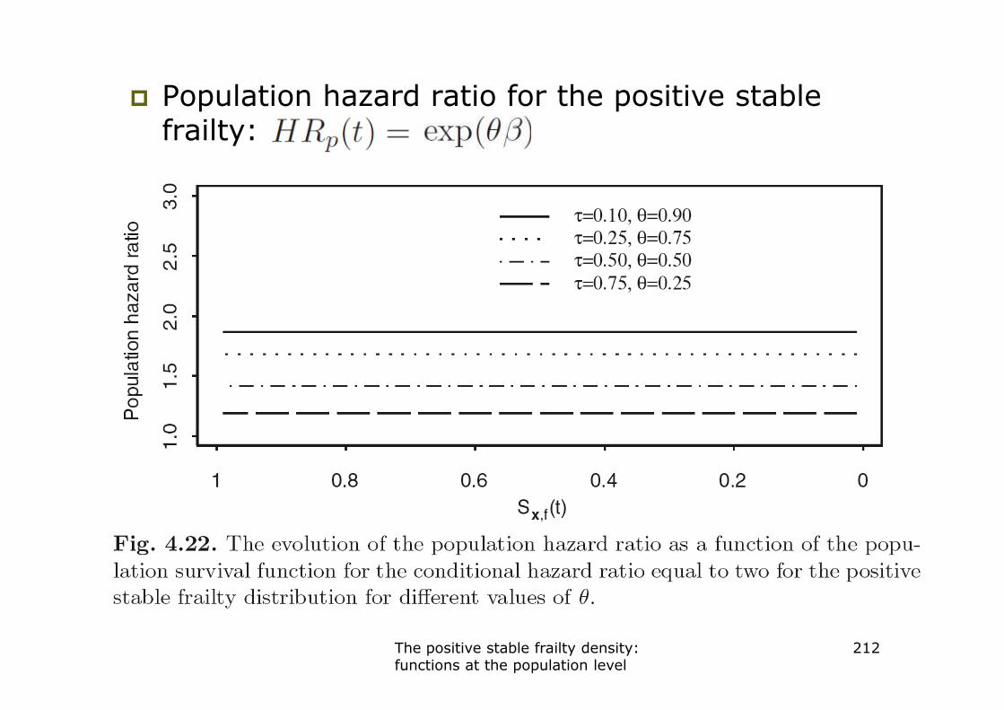
� Population hazard ratio for the positive stable frailty:
The positive stable frailty density: functions at the population level
212

An example: udder quarter infection data� See Example 4
� Binary covariate: heifer/multiparous ( is the heifer effect)
Weibull baseline hazard
Positive stable frailtyPositive stable frailty
� Maximising the marginal likelihood we obtain
� (se=0.052)
� (se=0.114)
� (se=0.351)
� (se=0.039)
An example: udder quarter infection data
213
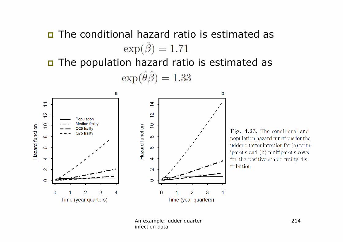
� The conditional hazard ratio is estimated as
� The population hazard ratio is estimated as
An example: udder quarter infection data
214

� First read in udder quarter infection data
#Read data
udder <- read.table("c:\\udderinfect.dat", header = T,skip=2)
coword<-order(udder$cowid)
cowid<-udder$cowid[coword]
Udder quarter infections and the positive stable frailty model in R
cowid<-udder$cowid[coword]
timeto<-4*(round(udder$timek[coword]*365.25/4))/365.25
stat<-udder$censor[coword];laktnr<-udder$LAKTNR[coword]
cluster<-as.numeric(levels(as.factor(udder$cowid)))
G<-length(cluster)
mklist<-function(clusternr){list(stat[cowid==clusternr], timeto[cowid==clusternr],laktnr[cowid==clusternr])}
clus<-lapply(cluster,mklist)
An example: udder quarter infection data in R
215

� Function to fit positive stable frailty model#p[1]=lambda, p[2]=rho, p[3]=beta, p[4]=theta
likelihood.posttab<-function(p){ll<-0
for (clusternr in (1:G)){
stat<-clus[[clusternr]][[1]];time<-clus[[clusternr]][[2]]
trt<-clus[[clusternr]][[3]];Di<-sum(stat)
SHij<-sum(exp(p[1])*time^(exp(p[2]))*exp(p[3]*trt))
part1<-sum(stat*log(exp(p[1])*exp(p[2])*(time^(exp(p[2])-1))*exp(p[3]*trt)))
part2<-Di*log(exp(p[4]))+Di*(exp(p[4])-1)*log(SHij)-SHij^(exp(p[4]))
part3<-0;if (Di==2) {part3<-log(1+((1-exp(p[4]))*SHij^(-part3<-0;if (Di==2) {part3<-log(1+((1-exp(p[4]))*SHij^(-exp(p[4]))/exp(p[4])))}
if (Di==3) {part3<-log(1+(3*(1-exp(p[4]))*SHij^(-exp(p[4]))/exp(p[4]))+( (exp(p[4])^(-2))*(2-exp(p[4]))* (1-exp(p[4]))*SHij^(-2*exp(p[4]))))}
if (Di==4) {part3<-log(1+(6*(1-exp(p[4]))*SHij^(-exp(p[4]))/exp(p[4]))+( (exp(p[4])^(-2))*(1-exp(p[4]))*(11-7*exp(p[4]))*SHij^(-2*exp(p[4])))+( (exp(p[4])^(-3))*(3-exp(p[4]))*(2-exp(p[4]))*(1-exp(p[4]))*SHij^(-3*exp(p[4]))))}
ll<-ll+(part1+part2+part3)}
-ll} An example: udder quarter infection data in R
216

� Results fit positive stable frailty model
lambda<-exp(t$estimate[1])
rho<-exp(t$estimate[2])
beta<-t$estimate[3]
theta<-exp(t$estimate[4])
> lambda
[1] 0.1766017[1] 0.1766017
> rho
[1] 2.129374
> beta
[1] 0.5374521
> theta
[1] 0.5285567
An example: udder quarter infection data in R
217

Updating (no covariates, positive stable frailty)� In general we have
� Applied to the positive stable frailty we have
� The updated density is not a positive stable density but is still a member of the power variance function family (see further)
Updating (no covariates, positive stable frailty)
218

Bivariate data: positive stable Laplace transform
�
with
�
Bivariate data: positive stable Laplace transform
219
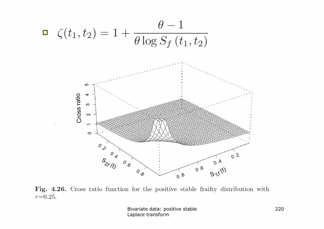
�
Bivariate data: positive stable Laplace transform
220

�
Bivariate data: positive stable Laplace transform
221

�
Bivariate data: positive stable Laplace transform
222

�
Bivariate data: positive stable Laplace transform
223

The lognormal frailty density� Introduced by McGilchrist (1993) as
� Therefore, for the frailty we have
The lognormal frailty density 224

� The lognormal frailty density: pictures
The lognormal frailty density 225

Statistical inference for the parametric lognormal frailty model� No explicit expression for Laplace transform …
difficult to compare
� Maximisation of the likelihood is based on numerical integration of the normally distributed frailtiesfrailties
Statistical inference for the parametric lognormal frailty model
226

An example: udder quarter infection data� See Example 4
� Binary covariate: heifer/multiparous ( is the heifer effect)Weibull baseline hazardLognormal frailty densityLognormal frailty density
� Maximising the marginal loglikelihood (using numerical integration: Gaussian quadrature –nlmixed procedure) we obtain
� (se=0.094)
� (se=0.135)
� (se=0.378)
� (se=0.610)
Statistical inference for the parametric lognormal frailty model
227

� Difficult to compare with e.g. the gamma frailty model since, for the lognormal frailty model, the mean and variance both depend on . We therefore convert the results to the density function of the median event time
Statistical inference for the parametric lognormal frailty model
228

Udder quarter infections and the lognormal frailty model in SASdata mast;infile 'c:\mastitis.dat' delimiter=',' firstobs=2;input LAKTNR censor rightk leftk cowid timek;if leftk=0 then leftk=0.001;if censor=1 then midp=(leftk+rightk)/2;if censor=0 then midp=rightk;y=1;
An example: udder quarter infection data in SAS
229
proc nlmixed data=mast qpoints=10 cov;ebetaxb = exp(beta1*LAKTNR + b);G_t = exp(-lambda*ebetaxb*(midp**g));f_t = (lambda*ebetaxb*g*midp**(g-1))*exp(-lambda*ebetaxb*(midp**g));if (censor=1) then lik=f_t;else if (censor=0) then lik=G_t;llik=log(lik);model y~general(llik);random b~normal(0,theta) subject =cowid;run;

The semiparametric frailty model
230

Overview� The semiparametric frailty model
� The marginal likelihood … a problem
� The EM-algorithm for the semiparametric frailty model
� The modified EM-algorithm
� An example: the DCIS (EM)
� The penalised partial likelihood approach for the semiparametric frailty model
� An example: the DCIS (PPL: normal, resp. loggamma, random effect)
� The performance of the PPL approach in estimating the heterogeneity parameter
Overview 231

The semiparametric frailty model� A semiparametric frailty model is a model with
unspecified (nonparametric) baseline hazard
with and unspecified
� For we will consider the one-parameter gamma and the lognormal frailty
The semiparametric frailty model 232

The marginal likelihood … a problem� We first discuss the one-parameter gamma frailty
� For parametric frailty models with gamma frailty distribution we maximised the marginal log like-lihood obtained from cluster contributions of form
� For the semiparametric frailty model, this is no longer possible since the baseline hazard is unspecified
The marginal likelihood … a problem 233

� Semiparametric survival models (Cox models) are typically fitted through partial likelihood maximisation
� We will study two techniques to fit semiparametric frailty models, which combine the partial likelihood maximisation idea (classical approach for the Cox model) with the fact that, since the random frailty terms are unobserved, since the random frailty terms are unobserved, we have incomplete information (where the EM approach can help)
� The EM-algorithm
� The penalised partial likelihood approach
The marginal likelihood … a problem 234

The EM algorithm for the semiparametric frailty model� The general idea is as follows
� The EM-algorithm iterates between an Expectation and Maximisation step
� In the Expectation step, expected values for the frailties are obtained, conditional on the observed information and the current parameter estimatesand the current parameter estimates
� In the Maximisation step, the expected values for the frailties are considered to be known (fixed offset terms), and partial likelihood is used to obtain new estimates
The EM algorithm for the semiparametric frailty model
235

� The full likelihood
Consider the full loglikelihood for observed
information and unobserved information
The EM algorithm for the semiparametric frailty model
236

� Maximisation step using instead of
� Replace and in by expected values and obtained in iteration k
� Profile to a partial likelihood
with the risk set corresponding to
� Maximise to obtain estimate
The EM algorithm for the semiparametric frailty model
237
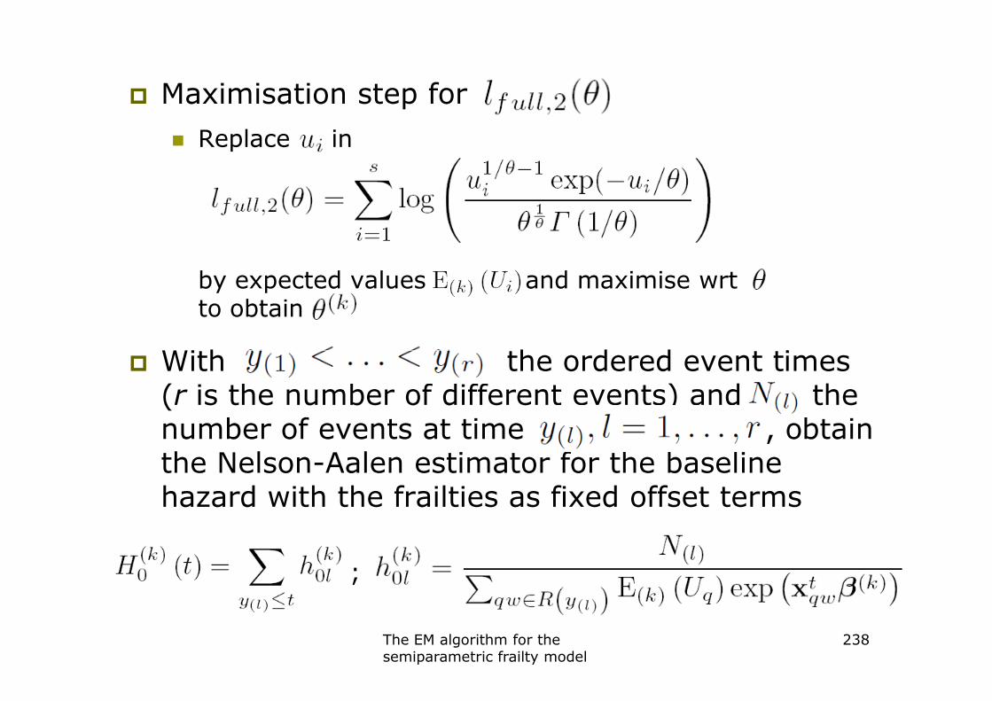
� Maximisation step for
� Replace in
by expected values and maximise wrt to obtain
With the ordered event times � With the ordered event times (r is the number of different events) and the number of events at time , obtain the Nelson-Aalen estimator for the baseline hazard with the frailties as fixed offset terms
The EM algorithm for the semiparametric frailty model
238
;

� The expectation step
We need expressions for and
� Obtain expectation conditional on current parameter estimate
and
� The conditional density of is (Bayes)
The EM algorithm for the semiparametric frailty model
239

� Working out the previous expression we get
with
� This corresponds to a gamma distribution with
parameters and
The EM algorithm for the semiparametric frailty model
240

� Therefore we have
� Furthermore, has a loggamma distribution and
thus, with the digamma functionthus, with the digamma function
The EM algorithm for the semiparametric frailty model
241

� Asymptotic variances of estimates are obtained as entries of the inverse of the observed information matrix obtained from the marginal loglikelihood
The EM algorithm for the semiparametric frailty model
242
…

The EM algorithm for the semiparametric frailty model
243

The modified EM-algorithm� Convergence rate can be improved by using
modified profile likelihood (Nielsen et al., 1992)
� The algorithm consists of two iteration levels
� Outer loop: maximisation forOuter loop: maximisation for
� Inner loop: maximisation for all other parameters conditional on chosen value
The modified EM-algorithm 244

The modified EM-algorithm 245

An example: the DICS (EM)� See Example 6
� We fit the semiparametric gamma frailty model
� Ductal Carcinoma in Situ (DCIS) is a type of � Ductal Carcinoma in Situ (DCIS) is a type of benign breast cancer
Breast conserving therapy with/without radiotherapy
Time to event: time to local recurrence
Large number of clusters (46) with small cluster size ( )
An example: the DICS (EM) 246

� Statistical analysis (using the SAS macro of Klein and Moeschberger (1997))
Radiotherapy effect =-0.63 (se=0.17)
=0.53 [0.38;0.71]
Heterogeneity =0.086 (se=0.80)
An example: the DICS (EM) 247

DCIS and the semiparametric gamma frailty model in SAS (Klein)%macro gamfrail(mydata,factors,initbeta,convcrit,leftend,stepsize,options,data1,data2,data3);use &mydata;…log(gamma((1/thetacr)+di[,i]))….
An example: DCIS in SAS 248
….
� Macro works for data with clusters with few events, such as DCIS
� Does not work when clusters have many events, as gamma((1/thetacr)+di[,i])) gets very large
� SAS macro requires IML

The PPL approach for the semiparametric frailty model� The PPL approach starts from model
with the frailty with variance and the random effect with variance
� The two main ideas are
� Random effects are considered to be just another set of parameters
� For values of far away from the mean (zero) the penalty term has a large negative contribution to the full data (partial) loglikelihood
The PPL approach for the semiparametric frailty model
249

� The PPL is
with
with
The PPL approach for the semiparametric frailty model
250

� Maximisation step of the PPL
� An iterative procedure using an inner and an outer loop
Inner loop: Newton Raphson procedure to maximise
for and (BLUP’s) given provisional
value for .
Outer loop: Obtain new value for using the current
estimates for and in the iteration process.
How this step works depends on the frailty density used
in the model. We will consider the outer loop for
random effects with a normal distribution and random
effects with a loggamma distribution.
The PPL approach for the semiparametric frailty model
251

� The inner loop of the PPL approach
� Some notation
� ( ) denotes the outer (inner) loop index
� is the estimate for at iteration
� and are estimates at iteration given
� At iteration step , the estimate is
with and
The PPL approach for the semiparametric frailty model
252

and
the inverse of matrix
The PPL approach for the semiparametric frailty model
253

� The outer loop for the PPL approach: normal random effect
� For normal random effects
� An estimate for is given by REML
where
� Convergence obtained when
is sufficiently small
The PPL approach for the semiparametric frailty model
254

� The variance estimates: normal random effect
The PPL approach for the semiparametric frailty model
255

The PPL approach for the semiparametric frailty model
256

� The outer loop for the PPL approach: loggamma random effect
� The loggamma distribution is
� Therefore, the penalty function is
The PPL approach for the semiparametric frailty model
257

� Outer loop: No REML estimator available!
Alternative: similar to modified EM-algorithm approach:
maximise marginal likelihood profiled for
� For fixed value , obtain estimates
by maximising PPL
� Plug in estimates in Nelson-Aalen estimator to obtain � Plug in estimates in Nelson-Aalen estimator to obtain
estimates of the (cumulative) baseline hazard
� Use estimates to obtain marginal likelihood
The PPL approach for the semiparametric frailty model
258

The PPL approach for the semiparametric frailty model
259

An example: the DCIS (PPL)� See Example 6
� We fit the PPL with normal random effect
� Radiotherapy effect =-0.63 (se=0.17)
= 0.53 [0.38;0.74]
� Heterogeneity =0.087 (se=0.80)
� We fit the PPL with loggamma random effect
� Radiotherapy effect =-0.63 (se=0.17)
= 0.53 [0.38;0.74]
� Heterogeneity =0.087 (se=0.80)
� The PPL can only be used to estimate , since the PPL considered as a function of increases (see figure)
An example: the DICS (EM) 260

� Statistical analysis (using the SAS macro of Klein and Moeschberger (1997))
Radiotherapy effect =-0.63 (se=0.17)
=0.53 [0.38;0.71]
Heterogeneity =0.086 (se=0.80)
An example: the DICS (EM) 261

An example: the DICS (EM) 262

DCIS and the semiparametric gamma frailty model in Rdcis<-read.table("c://dcis.dat", header=T)dcis.gamfrail <-coxph(Surv(lrectime,lrecst)~trt+frailty(hospno,dist="gamma",eps=0.00000001),outer.max=100,data=dcis)�summary(dcis.gamfrail)
coef se(coef) se2 Chisq DF p tr -0.628 0.167 0.167 14.1 1.00 0.00018
An example: DCIS in SAS 263
tr -0.628 0.167 0.167 14.1 1.00 0.00018frailty(hospno, dist = "g 11.5 7.82 0.16000
exp(coef) exp(-coef) lower .95 upper .95tr 0.534 1.87 0.385 0.741
Iterations: 10 outer, 29 Newton-RaphsonVariance of random effect= 0.0865 I-likelihood = -1005
Degrees of freedom for terms= 1.0 7.8 Rsquare= 0.034 (max possible= 0.866 )Likelihood ratio test= 34.8 on 8.82 df, p=5.69e-05Wald test = 14.1 on 8.82 df, p=0.112 ….

The performance of PPL in estimating heterogeneity � Simulation setting
� Number of clusters: 15 or 30
� Number of subjects/cluster: 20,40 or 60
� Constant hazard: 0.07 or 0.22
� Accrual/follow-up period: 5/3 years� Accrual/follow-up period: 5/3 years
resulting in 70% to 30% censoring
� Variance or : 0, 0.1, 0.2
� HR: 1.3
� 6500 data sets generated
The performance of PPL in estimating heterogeneity
264

� Size for semiparametric gamma frailty model
=0
The performance of PPL in estimating heterogeneity
265

� Testing for heterogeneity
� Hypothesis test: H0: =0 vs Ha: >0
-value in H0 is at boundary of parameter space
� Use mixture of and
The performance of PPL in estimating heterogeneity
266

Power For GammaFrailtymodelmodel
267
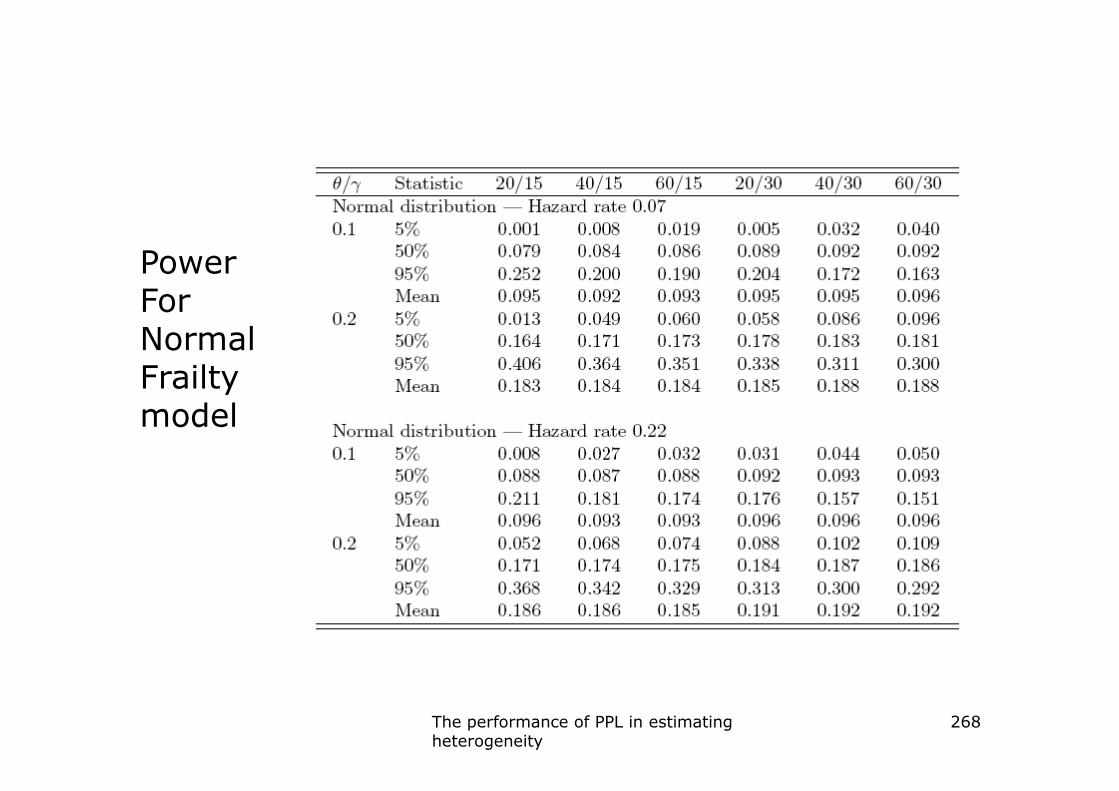
Power For NormalFrailtymodelmodel
The performance of PPL in estimating heterogeneity
268

Bayesian analysis of the semiparametric frailty model
269

Overview� Introduction
� Frailty model for grouped data and gamma process prior for the cumulative hazard
� Frailty model for observed event times and gamma process prior for the cumulative hazardgamma process prior for the cumulative hazard
� Examples
Overview 270

Introduction� Bayesian techniques can be used to fit frailty
models
Important references are
Kalbfleisch (1978): Bayesian analysis for the semiparametric Cox modelsemiparametric Cox model
Clayton (1991): Bayesian analysis for frailty models
Ibrahim et al. (2001): Bayesian survival analysis (book)
Introduction 271

� Metropolis algorithm: sampling from the joint (multivariate) posterior density of the parameters of interest
For semiparametric frailty model: a problematic approach since hazard rate at each event time is considered as a parameter
high dimensional sampling problem
(Metropolis no longer efficient)(Metropolis no longer efficient)
Gibbs sampling: sampling from posterior density of each parameter conditional on the other parameters (iterative procedure)
Introduction 272

Frailty model for grouped data and gamma process prior for H(t)� Consider the model
with actual value of
� We need the conditional posterior density of each parameter (conditional on all other parameters) We therefore needWe therefore need
� the list of all parameters involved
� the prior densities of the parameters
� the (conditional) data likelihood
� Grouped data: time axis is partitioned in z disjoint intervals
with
Frailty model for grouped data 273

� For a particular interval and a particular subject three situations are possible
(i) the subject experienced the event in
(ii) the subject did not experience the event in and is still at risk at
(iii) the subject is no longer in the study at time and is lost to follow-up in the interval
� The increase of the cumulative (unspecified) � The increase of the cumulative (unspecified) baseline hazard in is
For these increments (considered as parameters) we will assume an independent increments gamma process prior (see further)
Frailty model for grouped data 274

� The ‘parameters’ of interest are
the vector with the regression parameters
an hyperparameter
� To see how the conditional data likelihood for � To see how the conditional data likelihood for grouped data is constructed we look at a concrete example
Frailty model for grouped data 275

� Observed and grouped data: pictures
Frailty model for grouped data 276

� The likelihood contributions of the six subjects are
Frailty model for grouped data 277

� General expression for the conditional data likelihood is
� in terms of the contributions of the subjects
with
� in terms of the intervals
Frailty model for grouped data 278

� This is different from previous survival expressions since we only specify cumulative hazard increments (and not the baseline hazard itself).
The expression resembles the likelihood used for interval-censored data.
Frailty model for grouped data 279

� Specification of the prior densities (distributions)
� Independent increments gamma process for the cumulative baseline hazard
with an increasing continuous function such that
and independence between the increments
contained in
For the cumulative baseline hazard we have
with and
Note. Often a time-constant hazard and thus ;c large means variance small and
therefore strong prior belief in
Frailty model for grouped data 280

� ( )
improper uniform prior
�
� Clayton (1991)� Clayton (1991)
Gelman (2003)
Frailty model for grouped data 281

� Derivation of posterior densities: the general principle
with a -vector
and is the vector with component i
deleted
Frailty model for grouped data 282

Since (we assume inde-
pendence of prior densities) and since
does not depend on
unnormalised conditionalposterior density
Notes
(i) Normalising factor often difficult to obtain
(ii) If obtained the resulting posterior density does not take a form from which it is easy to sample
(iii) An approximation for the derived likelihood expression will lead to more simple conditional posterior densities from which sampling is easy
Frailty model for grouped data 283
posterior density

Frailty model for event times and gamma process prior for H(t)� To obtain an appropriate data likelihood in case of
(censored) event times, we use ideas developed for grouped data with intervals with the ordered event times
Frailty model for observed event times 284

� Approximation for the derived likelihood.
For instance, for the event time ,
For censored subjects the contribution is based on the
cumulative hazard corresponding to the sum of the cumulative hazard increments of all event times before the actual censoring time (like in grouped data)
Frailty model for observed event times 285

� This leads to the following likelihood expression
with
oror
with if and
This expression resembles the likelihood of Poisson distributed data
Frailty model for observed event times 286

� Prior densities: as before
� Posterior densities
� regression parameters
this density is logconcave adaptive rejection
sampling can be used to generate a sample
Frailty model for observed event times 287

� cumulative hazard increments
After a tedious derivation we obtainAfter a tedious derivation we obtain
Frailty model for observed event times 288

This is a gamma density
with
with the risk set at time
and the number of events at event time
sample from a gamma density
Frailty model for observed event times 289

� frailties
sample from a gamma density
� the hyperparameter with
difficult density, slice sampling is neededFrailty model for observed event times 290

� the hyperparameter with uniform on
difficult density, slice sampling is needed
� A similar discussion can be given for the normal frailty model based on Poisson likelihood
Frailty model for observed event times 291
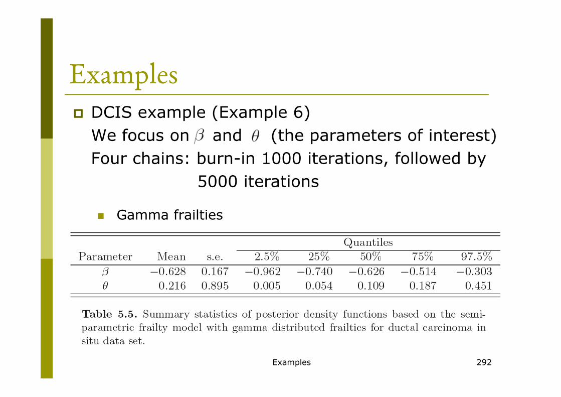
Examples� DCIS example (Example 6)
We focus on and (the parameters of interest)
Four chains: burn-in 1000 iterations, followed by
5000 iterations
� Gamma frailties
Examples 292

� Posterior densities – gamma frailties: pictures
Examples 293

� The trace – gamma frailties: pictures
Examples 294

� Normal random effects
Examples 295

� Posterior densities – normal random effects: pictures
Examples 296

� The trace – normal random effects: pictures
Examples 297

� Conclusion: Problem with convergence
(for , resp. )
� Udder infection data (Example 4) with normal random effects
Examples 298

� Posterior densities – normal random effects: pictures
Examples 299
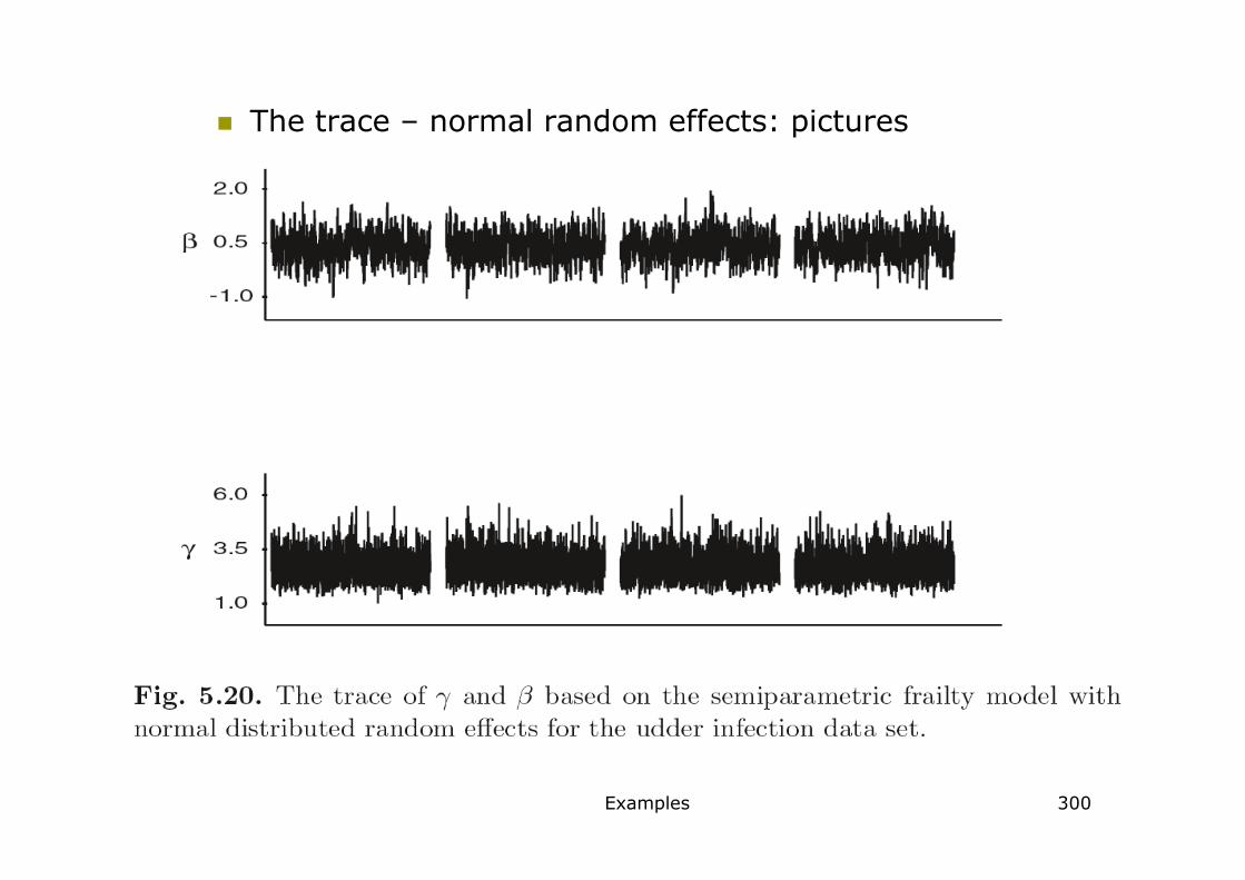
� The trace – normal random effects: pictures
Examples 300

� Conclusion: No problem with convergence
(for )
Examples 301

Multilevel and multifrailty models

Overview
� Multifrailty versus multilevel
Only one cluster, two frailties in cluster
� e.g., prognostic index (PI) analysis, with random center effect and ramdom PI effect
More than one clustering levelMore than one clustering level
� e.g., child mortality in Ethiopia with children clustered in village and village in district
� Modelling techniques
� Bayesian analysis through Laplacian integration
� Bayesian analysis throgh MCMC
� Frequentist approach through numerical integration
303Overview

Bayesian analysis through Laplacian integration
� Consider the following model with one clustering level
with the random center effectwith the random center effect
covariate information of first covariate, e.g. PI
fixed effect of first covariate
random first covariate by cluster interaction
other covariate information
other fixed effects
304Bayesian analysis through Laplacian integration

� Aim of Bayesian analysis: obtain posterior distributions for parameters of interest
� Ducrocq and Casella (1996) proposed a method based on Laplacian integration rather than Gibbs sampling
� Laplacian integration is much faster than Gibbs sampling, which makes it more suitable to their type of data, i.e., huge data sets in animal type of data, i.e., huge data sets in animal breeding, looking at survival traits
� Emphasis is placed on heritability and thus estimation of variance components
� Posterior distributions are only provided for variance components, fixed effects are only considered for adjustment
305Bayesian analysis through Laplacian integration

� The joint posterior density is given by
� with
the variance of the random centre effect
the variance of random covariate by cluster interactioninteraction
likelihood
� furthermore, we have the prior distributions
random effects are independent from each other
306Bayesian analysis through Laplacian integration

�and for the other prior parameters flat priors are assumed
�We leave baseline hazard unspecified, and therefore use partial likelihood (Sinha et al., 2003)
307Bayesian analysis through Laplacian integration

� The logarithm of the joint posterior density is then proportional to
� The posterior distribution of the parameters of interest can be obtained by integrating out other parameters
308Bayesian analysis through Laplacian integration

� No analytical solution available for
� Approximate integral for fixed value by Laplacian integration
� For fixed value we use notation
� First we obtain the mode of the joint posterior � First we obtain the mode of the joint posterior density function at
by maximising the logarithm of the joint posterior density wrt and (limited memory quasi-Newton method)
309Bayesian analysis through Laplacian integration

� We first rewrite integral as
and replace by the first terms of its Taylor expansion around the mode
� The second term of the Taylor expansion cancels
� For the third term we need the Hessian matrix
Bayesian analysis through Laplacian integration

� The integral is then approximately
� As has asymptotically a multivariate normal distribution with variance covariance matrix , distribution with variance covariance matrix , we have
Bayesian analysis through Laplacian integration

� The integral can therefore be simplified to
or on the logarithmic scale
� Estimates for and are provided by the mode of this approximated bivariate posterior density
� To depict the bivariate posterior density and determine other summary statistics by evaluating the integral on a grid of equidistant points
Bayesian analysis through Laplacian integration

� The values can be standardised by computing
with the distance between two adjacent points
� Univariate posterior densities for each of the two variance components can be obtained asvariance components can be obtained as
Bayesian analysis through Laplacian integration

� This discretised version of the posterior densities can also be used to approximate the moments
� The first moment for is approximated by
� In general, the cth moment is given by
Bayesian analysis through Laplacian integration

� From these non-central moments, we obtain
� The mean
� The variance
� The skewness
Bayesian analysis through Laplacian integration

Bayesian analysis through Laplacian integration: Example
� Prognostic index heterogeneity for a bladder cancer multicentre trial
� Traditional method to validate prognostic index
� Split database into a training dataset (typically 60% of the data) and validation dataset (remaining 40%)the data) and validation dataset (remaining 40%)
� Develop the prognostic index based on the training dataset and evaluate it based on the validation dataset
� Flaws in the traditional method
� How to split the data, at random or picking complete centers?
� This will always work if sample sizes are sufficiently large
� It ignores the heterogeneity of the PI completely
316Bayesian analysis through Laplacian integration

� We fit the following frailty model
with the overall prognostic index effect
the random hospital effect
the random hospital* PI interaction
and consider disease free survival (i.e., time to relapse or death, whatever comes first). death, whatever comes first).
� Parameter estimates
= 0.737 (se=0.0964)
= 0.095
= 0.016
317Bayesian analysis through Laplacian integration

� Interpreting the parameter estimates
� Good prognosis in center i,
� Poor prognosis in center i,
� Hazard ratio in center i,� Hazard ratio in center i,
� If for cluster i, , the mean of the distribution
with 95 % CI
� This CI refers to the precision of the estimated conditional hazard ratio
318Bayesian analysis through Laplacian integration

� Bivariate posterior density for
319Bayesian analysis through Laplacian integration

� Univariate posterior densities for
320Bayesian analysis through Laplacian integration

� Plotting predicted random center and random interactions effects
321Bayesian analysis through Laplacian integration

� Interpretation of variance component
� Heterogeneity of median event time quite meaningless, less than 50% of the patients had event, therefore rather use heterogeneity of five-year disease free percentage
� Fit same model with Weibull baseline hazard
leading to the following estimate
322Bayesian analysis through Laplacian integration

� The density of the five-year disease-free percentage
using
is then given by
where and FN standard normal
323Bayesian analysis through Laplacian integration

� The density of the five-year disease-free percentage
324Bayesian analysis through Laplacian integration

� Interpretation of variance component
� The hazard ratio for center i is given by
� Derive the density function for this expression.
� What are the 5th and 95th quantiles for this density assuming the parameter estimates assuming the parameter estimates
are the population parameters
325Bayesian analysis through Laplacian integration
= 0.737 (se=0.0964)
= 0.016

� We look for
� General rule
� Applied to
=lognormal with parameters and
326Bayesian analysis through Laplacian integration

� The density function for
327Bayesian analysis through Laplacian integration

� For lognormal distribution we have
� For the x% quantile of HR, , we have
� Therefore, the 5th and 95th quantiles are given by
328Bayesian analysis through Laplacian integration

Multilevel frailty models using a frequentist approach
� Consider the following model with two clustering levels
with the frailty term for cluster iwith the frailty term for cluster i
the frailty term for subcluster j nested in cluster i
We further assume that frailty terms are independent and
gamma distributed
329Multilevel frailty models using a frequentist approach

� The conditional likelihood is then given by
� The marginal likelihood for cluster i is
330Multilevel frailty models using a frequentist approach

� Integrating out the frailties analytically, we obtain
with the number of events in subcluster jnested in cluster i
number of events in cluster i
331Multilevel frailty models using a frequentist approach

� Taking the logarithm we obtain the marginal log-likelihood
� The marginal loglikelihood still contains the baseline hazard and cumulative baseline hazard
� Hazard functions are modeled using splines (Rondeau et al., 2006)(Rondeau et al., 2006)
� Cubic M-splines for baseline hazard function
� Integrated M-splines for baseline cumulative hazard
� Penalty term added to marginal likelihood to cont-rol the degree of smoothness of hazard function
332Multilevel frailty models using a frequentist approach

� The smoothing parameter can be chosen by visual inspection or by maximising a likelihood cross-validation criterion.
� The penalised marginal loglikelihood is then maximised using the Marquardt algorithm.
� For evaluation of the penalised marginal loglikelihood, the frailties corresponding to the loglikelihood, the frailties corresponding to the large clusters are integrated out numerically using Gaussian quadrature.
� This technique is implemented in the software package ‘frailtypack’, also available in R
333Multilevel frailty models using a frequentist approach

Frequentist approach for multilevel frailty model: Example
� Multilevel child mortality data (Example 12)
� Gender effect: =-0.137 (se=0.071)
HR (female versus male)= 0.87 [0.76;1.00]
� Variance of village frailties: 0.0450 (se=0.028) � Variance of village frailties: 0.0450 (se=0.028)
� Variance of district frailties: 0.0073 (se=0.00007)
334Bayesian analysis through Laplacian integration