Multivariate feature selection and hierarchical

classification for infrared spectroscopy:

serum-based detection of bovine spongiform

encephalopathy

Bjoern H. Menze1,2, Wolfgang Petrich2,3, Fred A. Hamprecht1,2

November 20, 2006

1 Interdisciplinary Center for Scientific Computing (IWR), University of

Heidelberg, Germany

2 Department of Physics and Astronomy, University of Heidelberg, Germany

3 Roche Diagnostics GmbH, Mannheim, Germany

Manuscript submitted to Analytical and Bioanalytical Chemistry.

1

Abstract

A hierarchical scheme has been developed to detect bovine spongiform

encephalopathy (BSE) in serum based on its infrared spectral signature.

In the first stage, binary subsets between samples originating from

diseased and non-diseased cattle are defined along known covariates within

the data set. Then, random forests are used to select spectral channels

on each subset, based on a multivariate measure of variable importance,

namely the Gini importance. The selected features are used to establish

binary discriminations within each subset by means of ridge regression.

At the second stage of the hierarchical procedure, the predictions from all

linear classifiers are used as input to another random forest that provides

the final classification.

When applied to an independent, blinded validation set of 160 further

spectra (84 BSE positives, 76 BSE negatives), the hierarchical classifier

reaches a sensitivity of 92% and a specificity of 95%. Compared to results

of an earlier study based on the same data, the hierarchical scheme per-

forms better than a linear discriminant analysis with features selected by

genetic optimization and a robust linear discriminant analysis, and per-

forms as well as or slightly better than a neural network and a support

vector machine.

Keywords: bovine spongiform encephalopathy, mid-infrared spectroscopy, diag-

nostic pattern recognition, ensemble classifier, random forest, Gini importance,

feature selection, hierarchical classification

2

1 Introduction

Fourier transform infrared spectroscopy (FTIR) has been attributed an impor-

tant role in biomedical research and application [1, 2, 3, 4, 5, 6]. Besides an

increasing number of FTIR imaging activities, in particular in the characteri-

zation of tissues [7], the mid-infrared spectroscopy of biological fluids has been

shown to reveal disease specific changes in the spectral signature, e.g. for bovine

spongiform encephalopathy [3], diabetes mellitus [2], the metabolic syndrome

[8], or rheumatoid arthritis [9].

In contrast to other diagnostic tests, on which the presence or absence of, for

example, the characteristic immunological reaction of a biomarker can easily be

recognized, the detection of such a characteristic change in the high-dimensional

spectral data remains in the realm of multivariate data analysis and pattern

recognition. Consequently, diagnostic tests which combine the spectroscopy

e.g. of molecular vibrations with a subsequent multivariate classification are

often referred to as “disease pattern recognition” or “diagnostic pattern recog-

nition” [10, 2, 9].

To ensure high performance of such a test, the robustness of this diagnos-

tic decision rule is of crucial importance. In chemometrics, popular concepts

for removing irrelevant variation in the data and regularizing the classifier in

ill-posed learning problems are the subset selection of relevant spectral regions

and the use of linear models.

In the following a hierarchical design of a classifier is proposed which com-

bines these two concepts in the example of the detection of bovine spongiform

encephalopathy (BSE) in infrared spectra of biofilms of bovine serum (data

section). A hierarchical decision rule is introduced, which explicitly considers

covariates in the data set, and which is based on random forests – a recently

3

proposed ensemble classifier [11] – and its entropy related feature importance

measure, the Gini importance (classifier section). We will illustrate how this

algorithm differs from other feature selection strategies, and discuss the rele-

vance of our findings on the given diagnostic task. Finally, we will compare the

performance with previous results of other chemometric approaches using the

same data set (results and discussion section). We would like to point out that

it is a strength of the manuscript that the feature selection and classification is

benchmarked against other methods on the basis of an identical data set.

2 Experiments and Data

2.1 Data

A total of 641 serum samples were acquired from confirmed BSE-positive (210)

or BSE-negative (211) cattle by the Veterinary Laboratory Agency (VLA), Wey-

bridge, UK and from BSE-negative cattle of a commercial abattoir in southern

Germany (220). All BSE-positive samples originated from cattle in the clinical

stage, i.e. the animals showed clinical signs of BSE and were subsequently shown

to be BSE-positive by histopathological examination. To the extent to which

this information was available (about 1/3 of the cases), all of the BSE-negative

samples originated from animals which were neither suspected to suffer from

BSE nor did the samples originate from a farm at which a BSE-infection had

previously occurred. With 641 samples originating from 641 cows this data set

represents one of the largest studies ever performed in biomedical vibrational

spectroscopy.

After thawing, 3µl of each sample were pipetted onto each of three dis-

posable silicon sample carriers using a modified COBAS INTEGRA 400 in-

4

strument1 and left to dry to reduce the strong infrared absorption caused by

water. Upon drying, the serum sample forms a homogenous film with a diam-

eter of 6 mm and a thickness of a few micrometers. Spectra were measured

in transmission using a Matrix HTS/XT spectrometer (Bruker Optics GmbH,

Ettlingen) equipped with a DLATGS detector. Each spectrum was recorded in

the wavenumber range from 500− 4000cm−1, sampled at a resolution of 4cm−1

(fig. 1). Blackman-Harris 3-term apodization was used and a zero-filling factor

of 4 was chosen. Finally, a spectrum was represented by vector of length 3629.

The three absorbance spectra of each sample measurement were corrected in-

dividually for the sample carrier background (for further details see ref. [12]).

Subsequently the spectra were normalized to constant area (L1 normalization)

in the region between 850cm−1 and 1500cm−1 and the mean spectrum of each

triplicate was calculated. The final smoothing and subsampling by a “binning”

(averaging) over adjacent channels was subject to the hyperparameter tuning

on each binary subset of the data (using a single bin-width “bw” for the whole

spectrum, see below). In contrast to other protocols in IR data processing, band

and high pass filters (such as Savitzky Golay) were not applied.

For the teaching2 of the classifier, 126 BSE-positive samples (from VLA)

and 355 BSE-negative samples (135 from VLA, 220 from the German abattoir)

were selected. Most of the teaching data were measured on a system at Roche

Diagnostics, but 60 of the samples were measured on a second system located

at the VLA, Weybridge (see also [12]). – A second, independent data set was

reserved for validation, comprising the spectra of another 160 serum samples

(84 positive, 76 negative, as randomly selected by the study site (VLA); all of

1COBAS INTEGRA is a trademark of a member of the Roche group2If not indicated otherwise, we will adhere to the spectroscopists’ terminology in the par-

titioning of the data set: The classification model is trained on the training data and itshyperparameters are adjusted on the test data. This process of training and testing is sum-marized as teaching. The final classifier is then validated on an independent validation set toassess the performance of the classifier.

5

Figure 1: Spectral data as a function of the wavenumber; median (line) andquartiles (dots) of the two classes are indicated. Top: Diseased (gray) andnormal (black) groups. Bottom: Groups after a channel-wise removal of themedian and a normalization to unit variance of the whole data set, as implicitlyperformed by most chemometric regression methods.

6

them acquired and measured at the VLA). This validation data set was retained

at Roche Diagnostic until the teaching of the classifier was finalized. Then the

classifier was applied to the validation data and the classification results were

reported to Roche Diagnostics, where the final comparison against the true

(post-mortem) diagnosis of the validation data was carried out.

2.2 Classification

On the given data, we defined eight binary subproblems, contrasting those BSE-

positive and negative samples that varied in one known covariate only (fig. 2)

such that each split between diseased and non-diseased specimen also repre-

sented a split over maximally one covariate within the data sets. On each of the

binary subset we optimized preprocessing, feature selection (using Gini impor-

tance) and linear classification individually, and finally induced the decisions on

the subsets in a second decision level (fig. 3). Concepts of both feature selection

by random forests and the hierarchical classification scheme are presented first,

followed by details on implementation and tuning procedures.

Feature selection by random forests

Decision trees are a very popular classifier both in biometry and machine learn-

ing, and have also found application in chemometrical tasks (see [13] and ref-

erences therein). A decision tree splits the feature space recursively until each

split holds training samples of one class only. A monothetic decision tree thus

represents a sequence of binary decisions on single variables.

Often, the pooled predictions of a large number of classifiers, trained on

slightly different subsets of the teaching data, outperform the decision of a sin-

gle classification algorithm which was optimally tuned on the full data set. This

is the idea behind ensemble classifiers. “Bootstrapping”, random sampling with

7

Figure 2: Scheme for the identification of binary subgroups. A classifier istrained to discriminate between pairs of “positives” and “negatives” which alsodiffer in maximally one covariate (similarity in covariates is expressed by symbolor color).

Figure 3: Architecture of the hierarchical classifier. For the prediction, a series ofbinary classification procedures is applied to each spectrum as a first step. Thesingle classifiers of each subgroup (from left to right) are individually optimizedwith respect to preprocessing, feature extraction and classification. To inducethe final decision concerning the state of disease, a nonlinear classifier is appliedto the binary output of all classifiers of the first level.

8

replacement of the teaching data, is one way to generate such slightly differing

training sets. “Random forest” is a recently proposed ensemble classifier that

relies on decision trees trained on such subsets [11, 14]. In addition to boot-

strapping, random forests also use another source of randomization to increase

the “diversity” of the classifier ensemble: “Random splits” [11] are used in the

training of each single decision tree, restricting the search for the optimal split

to a random subset of all features or spectral channels.

Random forests are a popular multivariate classifier which is benevolent to

train, i.e. which yields results close to the optimum without extensive tuning

of its parameters, and shows a classification performance comparable to other

algorithms such as support vector machines, neural networks, or boosting trees

on a number of data sets [15]. A superior behavior on micro-array data, often

resembling spectral data in sample size and feature dimensionality, has been

reported [16, 17, 18]. However, this superior classification performance was not

observed on the present data set and the initial training of a random forest on the

binary subproblems of the hierarchical classification procedure serves a differ-

ent purpose: It reveals information about the relevance of the spectral channels.

During training, the next split at the node of a decision tree (and thus the

next feature) is chosen so as to minimize a cost function which rates the purity

of the two subgroups arising from the split. Popular choices are the decrease

in misclassification or, alternatively, in the Gini impurity, an empirical entropy

criterion [19]. Both favor splits that separate the two classes completely – or at

least result in one pure subgroup – and assign maximal costs, if a possible split

is not able to unmix the two classes at all (fig. 4). Formally, Gini impurity and

(cross-) entropy can be expressed in the two-class case as

9

Gini∑

i=0,1 pi(1− pi)Entropy

∑i=0,1−pi log(pi)

with proportions p0 and p1 of samples from class 0 and class 1 within a separated

subgroup.

Recording the discriminative value of any variable chosen for a split during

the classification process by the decrease in Gini impurity, and accumulating

this quantity over all splits in all trees in the forest leads to the Gini importance

[11], a measure which indicates those spectral channels that were important at

any stage during the teaching of the multivariate classifier. The Gini importance

differs from the standard Gini gain as it does not report the conditional impor-

tance of a feature at a certain node in the decision tree, but the contribution of

a variable to all binary splits in all trees of the forest.

In practical terms, to obtain the Gini importance for a certain classifica-

tion problem, a random forest is trained and returning a vector which assigns

an importance to each channel of the spectrum. This importance vector often

resembles a spectrum itself (fig. 5) and can be inspected and checked for plau-

sibility. More importantly, it allows for a ranking of the spectral channels in

a feature selection. In our hierarchical classification scheme (fig. 3), the Gini

importance is used to obtain an explicit feature selection on each binary subset

in a wrapper approach together with a subsequent linear classification, e.g. by a

(discriminative) partial least squares regression or principal component regres-

sion.

So, rather than using random forests as a classifier, we advocate the use of

its feature importance to “upgrade” standard chemometric learners by a feature

selection according to the Gini importance measure.

10

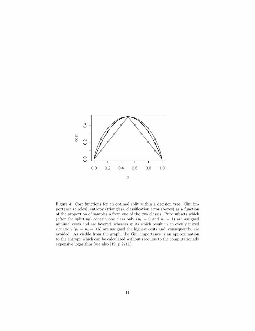
Figure 4: Cost functions for an optimal split within a decision tree: Gini im-portance (circles), entropy (triangles), classification error (boxes) as a functionof the proportion of samples p from one of the two classes. Pure subsets which(after the splitting) contain one class only (p1 = 0 and p0 = 1) are assignedminimal costs and are favored, whereas splits which result in an evenly mixedsituation (p1 = p0 = 0.5) are assigned the highest costs and, consequently, areavoided. As visible from the graph, the Gini importance is an approximationto the entropy which can be calculated without recourse to the computationallyexpensive logarithm (see also [19, p.271].)

11

Design of the hierarchical classifier

When a classifier is learned and its parameters are optimized on the training

data, statistical learning often assumes independent and identically distributed

samples. Unfortunately, experimental data do not necessarily justify these ideal

assumptions. Variations in the data and changes of the spectral pattern do

not always correlate with the state of disease only. For the particular case

under investigation, covariates such as breed of cattle or instrumental system-

to-system variation often also result in notable changes of the spectrum.

As a consequence, the differentiation between inter-class and intra-class vari-

ation becomes difficult for standard models which implicitly assume homogenous

distributions of the two classes, e.g. as in a linear discriminant analysis. How-

ever, influences of covariates and external factors on the data and their char-

acteristic changes of the spectra can be considered explicitly. If information on

these confounding factors is available both during teaching and validation and

these factors can be used as input features to the classifier, a multilayered or

stacked classification rule [20] can be designed to evaluate the combined infor-

mation from spectrum and factors appropriately (examples are given in [21, 22]).

If information on covariates is only available during teaching, this information

can still be leveraged in the design of the classifier. A mixture discriminant

analysis (MDA) [19], for example, provides means to extend linear discriminant

analysis to a nonlinear classifier. By introducing additional Gaussian proba-

bility distributions in the feature space, MDA allows one to explicitly model

subgroups which are distinguished by different levels of the (discrete) external

factors. The final decision is induced from the assessed probabilities, so – in

a two-level architecture – the MDA is often also referred to as a “hierarchical

mixture of experts” [19].

In the approach presented here, a similar hierarchical strategy is pursued.

12

However, instead of modeling probability distributions of subgroups, the de-

cision boundaries between positive and negative (diseased and non-diseased)

samples of the subgroups are taught directly (fig. 2). In the feature space, this

procedure generates a number of decision planes which partition the space into a

number of high dimensional regions. Samples within a certain region are coded

by a specific binary sequence, according to the outcome of all binary classifiers

of this first step. A second classifier, assigning a class label to each of these

volumes, is trained on these binary codes and provides a final decision about

the state of the disease. Two-layer-perceptrons are based on similar concepts.

Nevertheless, in the hierarchical rule presented here, the binary decisions of the

first level are explicitly adapted to interclass differences of subgroups defined

by the covariates and, in the the second level, a nonlinear classifier is employed

(fig. 3) to assure separability of nonlinear problems also in a two-level design.

To this end, we used a method which is particularly suited to induce decisions

on categorical and binary data, namely binary decision trees. Considering the

high variability of single decision trees, we have also preferred to use the ran-

dom forests ensemble at this stage. Thus we have obtained an approximation

to the posterior probability, rather than the dichotomous decision of the single

decision tree as the final decision of our hierarchical classifier.

Overall, compared to the generative MDA and the discriminative perceptron

which both allow for sound optimization of the classification algorithm in a

global manner, the hierarchical approach presented here is a mere ad-hoc rule.

The hierarchical design, however, allows the tuning of all three steps of the data

processing – preprocessing, feature selection, and classification – individually

and to explicitly consider the knowledge about covariates in the data.

13

Implementation and training

The origin of the samples and the two instrumental systems in England and

Germany were considered as covariates within the data set. The subgroups

comprised between 40 and 421 samples, with a median of 130.5.

For each binary subproblem, a number of factors in preprocessing, feature

selection and classification were tested and optimized individually, in a global

tuning procedure. The performance was assessed by a 10-fold cross-validation

of the classification error using the teaching set only.

The following factors (bw, Psel, Clmeth) were considered: In preprocessing,

a binning was tested from one to ten channels (bw = 1, 3, 5, 10) to obtain down-

sampled and smoothed feature vectors. In the feature selection, random forests

were learned on all binary subsets (using the implementation of ref. [23] with

the following parameters: mtry = 60, nodesize = 1, 3000 trees). Data sets

were defined which comprised the top 5%, 10% and 15% of the input features,

ranked according to the obtained Gini importance (resulting in test set com-

prising between 19 and 544 spectral features Psel, depending on the preceding

binning). For classification, partial least squares (PLS), principal component

regression (PCR), ridge regression (also termed penalized or robust discrim-

inant analysis) and standard linear discriminant analysis (LDA) were tested

(Clmeth = PLS, PCR, ridge, LDA). For these classifiers, the optimal split pa-

rameter was adapted according to the least fit error on the training set and

the respective hyperparameters (PLS & PCA dimensionality λ = 1 . . . 12, ridge

penalty λ = 2−5...5 [19]) were tuned via an additional internal 10-fold cross-

validation.

After the optimal parametrization was found in the first level, all binary

14

classifiers were trained on their respective subsets and their binary predictions

on the rest of the data set were recorded. Predictions for the samples of the

subsets themselves were determined by a 10-fold cross-validation. The outcome

of this procedure was a set of binary vectors of length eight as compact repre-

sentations for each spectrum of the teaching data. A nonlinear classifier was

trained on these vectors (random forest, initial experiments with bagging trees

yielded similar results) and optimized according to the out-of-bag classification

error.

All computing was performed using the programming language R [24] and

libraries which are freely available from cran.r-project.org, in particular the

randomForest package [23]. On a standard PC, the training of the random

forest was performed within seconds. The tuning of all 8 ∗ 4 ∗ 3 ∗ 4 combinations

of the predefined factor levels was in the range of hours. Once the design of

the hierarchical classifier was fixed, the training was done within minutes, and

the final classification of the blinded validation data was performed (nearly)

instantaneously.

3 Results and Discussion

Feature selection

To compare the Gini importance with standard measures, univariate statistical

tests were also applied to the data of the binary subproblems (fig. 5). Differences

between the model based T-test and a nonparametric Wilcoxon-Mann-Whitney

test are hardly noticeable (see fig. 5, top, for a representative example). Spectral

channels with an obvious separation between diseased and non-diseased chan-

nels (fig. 1, bottom) usually also score high in the multivariate Gini importance.

15

Figure 5: Importance measures on binary subset of the training data. Top:univariate tests for group differences, probabilities from T-test (black) andWilcoxon-Mann-Whitney test (gray). Shown is the negative logarithm of thep-value – low entries indicate irrelevance, high values report high importance.Middle: random forest Gini importance (arbitrary units). Bottom: direct com-parison of ranked Gini importance (black) and ranked T-score (gray). Horizon-tal lines (dotted) indicate optimal threshold on Gini importance.

16

However, differences become easily visible when ranking the spectral channels

according to multivariate Gini importance and p-values of the univariate tests,

respectively (fig. 5, bottom). Regions which had a complete overlap between

the two classes (fig. 1, bottom), and therefore no importance at all according

to the univariate tests, were often considered to be highly relevant by the mul-

tivariate measure (compare figs. 1 & 5: e.g. 1300cm−1, 3000cm−1), indicating

higher-order dependencies between variables. Conversely, regions which reveal

only slight drifts in the baseline were assigned modest to high importance by

the rank-ordered univariate measures, although known to be irrelevant from a

biochemical perspective (fig. 5: 1800 − 2700cm−1). Compared with the selec-

tion of the multivariate classifiers from [12], as obtained on the same data set,

similarities between the optimal selections from the Gini importance and the

earlier results could be observed (fig. 6, bottom).

All linear classifiers in the first level of the hierarchical rule differed in the

influence of the covariates on their respective subproblem. However, all were

optimized to separate diseased and non-diseased samples. So, inspecting the

regions that were chosen by the majority (≥ 50%) of the binary subgroup clas-

sifiers should primarily reveal disease specific differences (fig. 6). Highly rele-

vant regions are found around 1030 cm−1, which is known to be a characteristic

absorption of carbohydrates, and at 2955 cm−1, i.e. the asymmetric C − H

stretch vibration of −CH3 in fatty acids in agreement with the earlier studies

[3, 12, 25, 6]. Other major contributions can be found at 1120, 1280, 1310, 1350,

1460, 1500, 1560 and 1720 cm−1 (fig. 6).

Classifier

Ridge regression yielded the best results for most of the binary classification

subproblems during teaching of the classifiers. On average it performed 1-2%

17

Figure 6: Spectral regions chosen by the different classification strategies, alongthe frequency axis. Top: Histogram (frequency, see bar on the right side) ofchannel selection by random forest importance on one of the eight subproblems(RF). Bottom: selection of classifiers from [12], linear discriminant analysis(LDA), robust discriminant analysis (R-LDA), support vector machines (SVM),artificial neural networks (ANN).

18

Method Sensitivity (%) Specificity (%)LDA 82 93R-LDA 80 88SVM 88 99ANN 93 93meta classifier 93 96RF 92 95

Table 1: Sensitivity and specificity of classifiers from [12] and from randomforest based hierarchical rule (RF), when applied to the independent validationset (84 BSE positive, 76 BSE negative)

better than PLS, PCR and LDA (usually in this order). The comparably poor

performance of LDA, i.e. the unregularized version of the ridge in a binary

classification, indicates that even after binning and random forest selection, the

data was still highly correlated. To keep the architecture of the hierarchical

classifier as simple as possible, ridge regression was fixed for all binary class

separations in the first level.

Parameters for binning and feature selection were chosen individually for

each subproblem, comprising 5%-10% percent of the features after a binning by

five or ten channels. The high level of binning reflects the impact of apodiza-

tion and zero-filling, the spectrometer resolution and in particular the typical

linewidths of the spectral signatures of approx. 10cm−1 This reduced the dimen-

sionality of the classification problem by up to two orders of magnitude for all

subproblems (19 to 106 features, median 69) as compared to 3629 data points

in each original spectrum.

The final training yielded a sensitivity of 92% and a specificity of 96% within

the training set (out-of-bag-error of the random forest in the second level).

19

Validation

After having applied the classifier to the pristine validation data set the un-

blinding revealed that 77 of 84 serum samples originating from BSE-positive

cattle and 72 of 76 samples originating from BSE-negative cattle were identified

correctly. Numerically, these numbers correspond to a sensitivity of 92% and

a specificity of 95%. A slight improvement can be found compared to two of

the four individual classifiers in [12], namely the linear discriminant analysis

with features selected by genetic optimization, and the robust linear discrimi-

nant analysis (see table 1). Results are comparable to or slightly better than

the neural network or the support vector machine. Preliminary results from

a subsequent test of all five classifiers on a bigger data set (220 BSE positive

samples, 194 BSE negatives), confirm this tendency of the random forest based

classifier.

On the present data set, the hierarchical classifier performs nearly as well as

the meta classifier from [12] which combines the decisions of all four classifiers

(table 1). When extending the meta rule by the decisions of the classifier pre-

sented in this manuscript, the diagnostic pattern recognition approach reached

a specificity of 93.4% and a sensitivity of 96.4%. Comparing these number with

the results presented in [12] we find an increase in sensitivity at the expense

of a decrease in specificity. Of course, this desirable exchange of sensitivity

and specificity depends on the particular choice of the decision rule and we

had stringently followed the rule set up in [12] in order to provide an unbiased

comparison.

20

4 Conclusions

A hierarchical classification architecture is presented as part of a serum-based

diagnostic pattern recognition testing for BSE. The classification process is sepa-

rated in decisions on subproblems arising from the influence of covariates on the

data. In a first step, all procedures in data processing – preprocessing, feature

selection, linear classification – are optimized individually for each subprob-

lem. In a second step, a nonlinear classifier induces the final decision from the

outcome of these sub-classifiers. Compared to other established chemometric

classification methods, the presented approach performed comparably or better

on the given data.

The use of the random forest Gini importance as a measure for the con-

tribution of each variable to a multivariate classification process, allows for a

feature ranking which is fast and computationally efficient compared to other

global optimization schemes. Beside its value in the diagnostic interpretation

of the importance of certain spectral regions, the methods readily allow for an

additional regularization of any standard chemometrical regression method by

a multivariate feature selection.

Acknowledgements

The authors acknowledge the contributions of W. Kohler, T. Martin, and J. Mocks,

as well as partial financial support under grant no. HA-4364 from the DFG (Ger-

man National Science Foundation) and the Robert Bosch GmbH.

21

References

[1] H.-U. Gremlich and B. Yan, editors. Infrared and Raman spectroscopy of

biological materials, volume 24 of Practical Spectroscopy Series. Marcel

Dekker Publisher, New York, 2001.

[2] W. Petrich, B. Dolenko, J. Fruh, M. Ganz, H. Greger, S. Jacob, F. Keller,

A. E. Nikulin, M. Otto, O. Quarder, R. L. Somorjai, A. Staib, G. Werner,

and H. Wielinger. Disease Pattern Recognition in Infrared Spectra of

Human Sera with Diabetes Mellitus as an Example. Applied Optics,

39(19):3372–79, 2000.

[3] P. Lasch, J. Schmitt, M. Beekes, T. Udelhoven, M. Eiden, H. Fabian,

W. Petrich, and D. Naumann. Ante-mortem identification of bovine spongi-

form encephalopathy from serum using infrared spectroscopy. Analytical

Chemistry, 75(23):6673–78, 2003.

[4] D. Naumann. FT-infrared and FT-Raman spectroscopy in biomedical re-

search. Applied Spectroscopy Review, 36(2-3):238–198, 2001.

[5] W. Petrich. Mid-infrared and Raman spectroscopy for medical diagnostics.

Applied Spectroscopy Review, 36(2-3):181–237, 2001.

[6] H. Fabian, P. Lasch, and D. Naumann. Analysis of biofluids in aqueous

environment based on mid-infrared spectroscopy. Journal of Biomedical

Optics, 10(3):1–10, 2005.

[7] C. Beleites, G. Steiner, M.G. Sowa, R. Baumgartner, S. Sobottka,

G. Schackert, and R. Salzer. Classification of human gliomas by infrared

imaging spectroscopy and chemometric image processing. Vibrational Spec-

troscopy, 38(1-2):143–149, 2005.

22

[8] J. Fruh, S. Jacob, B. Dolenko, H.-U. Haring, R. Mischler, O. Quarder,

W. Renn, R. Somorjai, A. Staib, G. Werner, and W. Petrich. Diagnosing

the predisposition for diabetes mellitus by means of mid-IR spectroscopy.

Proceedings of SPIE, 4614:63–69, 2002.

[9] A. Staib, B. Dolenko, D.J. Fink, J. Fruh, A. E. Nikulin, M. Otto, M. S.

Pessin-Minsley, O. Quarder, R.L. Somorjai, U. Thienel, G. Werner, and

W. Petrich. Disease pattern recognition testing for rheumatoid arthritis

using infrared spectra of human serum. Clinical Chimica Acta, 308(1-2):79–

89, 2001.

[10] U. Himmelreich, R.L. Somorjai, B. Dolenko, O.C. Lee, H.M. Daniel,

R. Murray, C.E. Mountford, and T. C. Sorrell. Rapid identification of

candida species by using nuclear magnetic resonance spectroscopy and

a statistical classification strategy. Applied Environmental Microbiology,

69(8):4566–74, 2003.

[11] L. Breiman. Random forests. Machine Learning Journal, 45:5–32, 2001.

[12] T.C. Martin, J. Moecks, A. Belooussov, S. Cawthraw, B. Dolenko, M. Ei-

den, J. Von Frese, W. Kohler, J. Schmitt, R. L. Somorjai, T. Udel-

hoven, S. Verzakov, and W. Petrich. Classification of signatures of Bovine

Spongiform Encephalopathy in serum using infrared spectroscopy. Analyst,

129(10):897 – 901, 2004.

[13] A. Myles, R. Feudale, Y. Liu, N. Woody, and S. Brown. An introduction

to decision tree modelling. Journal of Chemometrics, 18(6):275–285, 2004.

[14] V. Svetnik, A. Liaw, C. Tong, J. C. Culberson, R. P. Sheridan, and B. P.

Feuston. Random Forest: A Classification and Regression Tool for Com-

pound Classification and QSAR Modeling. Journal of Chemical Informa-

tion and Computer Sciences, 43(6):1947–58, 2003.

23

[15] David Meyer, Friedrich Leisch, and Kurt Hornik. The support vector ma-

chine under test. Neurocomputing, 55(1-2):169–186, 2003.

[16] S. Li, A. Fedorowicz, H. Singh, and S.C. Soderholm. Application of the

random forest method in studies of local lymph node assay based skin sensi-

tization data. Journal of chemical information and modeling, 45(4):952–64,

2005.

[17] R. Diaz-Uriarte and S. Alvarez de Andres. Gene selection and classification

of microarray data using random forest. BMC Bioinformatics, 7(3), 2006.

[18] H. Jiang, Y. Deng, H.-S. Chen, L. Tao, Q. Sha, J. Chen, C.-J. Tsai, and

S. Zhang. Joint analysis of two microarray gene-expression data sets to

select lung adenocarcinoma marker genes. BMC Bioinformatics, 5(81),

2004.

[19] T. Hastie, R. Tibshirani, and J. Friedman. The Elements of Statistical

Learning. Springer Series in Statistics. Springer, New York, 2001.

[20] D.H. Wolpert. Stacked generalization. Neural Networks, 5(2):241–259,

1992.

[21] J. Schmitt and T. Udelhoven. Use of artificial neural networks in biomedical

diagnostics. In H.-U. Gremlich and B. Yan, editors, Infrared and Raman

spectroscopy of biological materials, volume 24 of Practical Spectroscopy

Series, pages 379–420. Marcel Dekker Publisher, 2001.

[22] K. Maquelin, C. Kirschner, L.-P. Choo-Smith, N. A. Ngo-Thi, T. van

Vreeswijk, M. Stammler, H. P. Endtz, D. Bruining, H. A. Naumann, and

G. J. Puppels. Prospective study of the performance of vibrational spectro-

scopies for rapid identification of bacterial and fungal pathogens recovered

from blood cultures. Journal of Clinical Microbiology, 41(1):324–329, 2003.

24

[23] A. Liaw and M. Wiener. Classification and Regression by randomForest.

R News, 2(3):18–22, 2002.

[24] R. Ihaka and R. Gentleman. R: A language for data analysis and graph-

ics. Journal of Computational and Graphical Statistics, 5(3):299–314, 1996.

http://www.r-project.org/.

[25] J. Schmitt, P. Lasch, M. Beekes, T. Udelhoven, M. Eiden, H. Fabian,

W. Petrich, and D. Naumann. Ante mortem identification of BSE from

serum using infrared spectroscopy. Proceedings of SPIE, 5321:36–43, 2004.

25