multivariate analyses of carcass traits for angus cattle...

July 26, 20061

Running head : PRINCIPAL COMPONENTS FOR CARCASS TRAITS2

Multivariate analyses of carcass traits for Angus cattle3

fitting reduced rank and factor-analytic models4

Karin Meyer5

Animal Genetics and Breeding Unit1, University of New England, Armidale NSW 2351,6

Australia7

E-mail :[email protected]

Phone : +61 2 6773 3331Fax : +61 2 6773 3266

8

1AGBU is a joint venture between the NSW Department of Primary Industries and the University of New

England

K.M. July 26, 2006 Principal components for carcass traits

Abstract9

Multivariate analyses of carcass traits for Angus cattle, consisting of 6 traits recorded10

on the carcass and 8 auxiliary traits measured by ultra-sound scanning of live animals,11

are reported. Analyses were carried out by restricted maximum likelihood, fitting a12

number of reduced rank and factor-analytic models for the genetic covariance matrix.13

Estimates of eigen-values and -vectors for different orders of fit are contrasted and14

implications on the estimates of genetic variances and correlations are examined.15

Results indicated that at most 8 principal components were required to model the16

genetic covariance structure among the 14 traits. Selection index calculations sug-17

gested that the first 7 of these PCs sufficed to obtain estimates of breeding values for18

the carcass traits without loss in expected accuracy of evaluation. This implied that19

the number of effects fitted in genetic evaluation for carcass traits can be halved by20

estimating breeding values for the leading principal components directly.21

2


1 Introduction22

Characteristics of carcass quality are of considerable importance in genetic improvement23

programmes for beef cattle. Hence, genetic evaluation schemes, such as BREEDPLAN in24

Australia (Graser et al., 2005), generally provide estimated breeding values (EBVs) for25

several carcass traits. As true carcass measurements can only be obtained at slaughter,26

most information contributing to genetic evaluation of stud animals is provided by corre-27

sponding traits measured on live animals via ultra-sound scanning. Generally, these traits28

are of little interest in their own right, and corresponding EBVs are not published.29

BREEDPLAN comprises 22 and more traits in a multivariate genetic evaluation scheme. Of30

these, 14 represent carcass measures, but only 6 EBVs for carcass traits per se are reported.31

The other traits, measured on young, live animals, represent 3 measures of ‘fatness’ and32

a measure of lean meat yield. As heifers and steers have different patterns of growth33

and protein deposition than bulls, variances and heritabilities for the same measure on34

animals of different sex differ and within-trait, between-sex genetic correlations are less35

than unity (Meyer and Graser, 1999). Hence, records on different sexes (heifers and steers36

versus bulls) are treated as different traits, yielding a total of 8 auxiliary carcass traits in37

the analysis. Genetic correlations between several of these traits are moderately high to38

high, 0.7 or above, in particular for ’fatness’ characteristics recorded on the same animal39

and between records for the same measure on different sexes.40

Estimation of genetic parameters for carcass traits per se has been hampered by the small41

number of records available. Conversely, computational requirements and problems with42

reliable estimation of large numbers of covariance components simultaneously have severely43

limited multivariate analyses of all traits together. For instance, Reverter et al. (2000) em-44

ployed 96 tri-variate, two four-variate and one six-variate analysis to estimate the complete45

genetic covariance matrix for the 14 carcass measures in BREEDPLAN. However, recent46

improvements in computing hardware available together with advances in methodology47

to model higher dimensional data more parsimoniously (Kirkpatrick and Meyer, 2004)48

and more stable algorithms for restricted maximum likelihood (REML) estimation (Meyer,49

2006a), have made such analyses feasible.50

3


Any set of correlated traits can be transformed into a set of new variables which are linear51

combinations of the original traits, are uncorrelated, and successively explain a maximum52

amount of variation. These new variables are generally referred to as principal compo-53

nents (PC), and are commonly reported in descending order of the amount of variation54

attributed to them. For highly correlated traits, the first few PCs then explain the bulk55

of variation, while the remaining PCs explain little or almost no variation. This implies56

that they provide virtually no information which is not already contained in the leading57

PCs, and that they can be ignored. This is the principle underlying the use of PCs as a58

dimension reduction technique. Recently, application at a genetic level has been suggested59

to reduce the number of EBVs to be estimated and the number of parameters to model the60

genetic covariance structure (Kirkpatrick and Meyer, 2004).61

Earlier analyses showed that 5 to 6 PCs were required to model the genetic covariance62

structure among the 8 scan traits, but that the first 3 or 4 of these sufficed to summarise63

genetic differences between animals, explaining 97% (3 PCs) to 98.7% (4 PCs) of genetic64

variation (Meyer, 2005a). This paper presents REML estimates of genetic parameters for65

carcass characteristics from multivariate analyses considering all 14 traits simultaneously,66

fitting reduced rank and factor analytic (FA) models. In addition, the scope for dimension67

reduction in genetic evaluation for carcass traits of beef cattle by considering the leading68

principal components only is examined.69

2 Material and methods70

2.1 Data71

Data consisted of records for carcass characteristics of Australian Angus cattle, extracted72

from the National Beef Recording Scheme data base in May 2005. These comprised 673

carcass traits, recorded at slaughter, and records for 4 correlated measures, recorded on74

live animals by ultra-sound scanning. Traits recorded on the carcass (C.) as well as on live75

animals were eye muscle area (EMA), intra-muscular fat content (IMF), and fat depth at76

the 12/13th rib (RIB) and the P8 rump site (P8). In addition, carcass weight (C.WT) and77

4


percentage retail beef yield (C.RBY) were recorded at slaughter.78

The majority of carcass measures were collected from abattoirs under a meat quality re-79

search project by the Australian Co-operative Research Centre for Cattle and Beef Indus-80

try conducted between 1994 and 1999; see Reverter et al. (2000) for details. Following81

Reverter et al. (2000), records for C.EMA taken by real time ultra-sound up to 14 days82

prior to slaughter were accepted as ‘carcass’ measurements. Additional records for C.WT,83

C.RIB and C.P8 from a small number of progeny testing herds, predominantly taken from84

2000 onwards, were available and included in the analysis. All carcass traits were recorded85

on heifers or steers.86

Scan traits were recorded in the field by accredited operators. As is standard practice in87

genetic evaluation of beef cattle in Australia (Graser et al., 2005), records for heifers or88

steers (H.) and bulls (B.) were treated as separate traits. Only scan records taken between89

300 and 700 days of age were considered. Extraction of scan records was aimed at selecting90

records for animals which had close genetic links with animals which had carcass traits91

recorded. Hence, only scan records in their herds of origin were considered. For these92

herds, all contemporary groups (CG) which contained progeny of sires of animals with93

carcass records were identified, and all records in these CG selected. There were too few94

animals in the data which had C.RBY or C.IMF as well as H.IMF records to obtain reliable95

estimates of the respective residual covariances. Hence H.IMF records for these animals96

were eliminated. After further basic edits, this yielded 121924 records on 30427 animals.97

Table 1 gives details for the 14 individual traits.98

2.2 Estimation of variance components99

Analyses fitted a simple animal model, including all pedigree information available for up100

to five generations backwards. Prior to analyses, pedigrees were ‘pruned’, i.e. any parents101

which did not contribute any information, because they had a single offspring only and no102

records themselves, were treated as unknown. This was done recursively, yielding 15501103

parents to be included, i.e. a total of 45928 animal genetic effects for each trait in the104

model of analysis. Animals in the data were progeny of 1024 sires and 12727 dams.105

5


Fixed effects fitted for scan traits were contemporary groups (CG), birth type (single vs.106

twin) and a dam age class (heifers vs. cows), the so-called ‘heifer factor’. CG were defined107

as herd-sex-management group-date of recording subclasses, with CG subdivided further108

if the range of ages in a subclass exceeded 60 days. Furthermore, age at recording, nested109

within sex, and age of dam were fitted as a linear and quadratic covariables. This resulted110

in a ‘double’ correction for ages, which was considered necessary as neither the covariable111

nor the fixed effect classification alone accounted for all age differences.112

Carcass traits were pre-adjusted prior to analyses, using the multiplicative adjustments113

of Reverter et al. (2000). C.WT records were adjusted to a slaughter age of 650 days,114

while the other carcass traits were standardised to a C.WT of 300 kg. Means (± standard115

deviation) of pre-adjusted records were 335.4± 52.8 kg, 62.7± 11.5 cm2, 5.374± 1.81 %,116

65.5±3.1 %, 12.28±5.04 mm and 8.99±4.36 mm for C.WT, C.EMA, C.IMF, C.RBY, C.P8117

and C.RIB, respectively. The model for carcass traits then included CG as the only fixed118

effect. For data from the research project, CG were defined as herd of origin-kill regime-sex119

of animal subclasses, with the term ‘kill regime’ representing a combination of date of kill,120

abattoir, finishing regime and target market. For the progeny test records, CG were simply121

slaughter date-herd of origin-sex of animal subclasses.122

Estimates of genetic and residual (co)variance matrices were obtained by REML from mul-123

tivariate analyses considering all 14 traits. In addition to a ‘standard’ multivariate analy-124

sis, denoted as F14, which assumed the genetic covariance matrix (ΣG) to be unstructured125

with 105 distinct covariance components, a number of analyses modelling the genetic dis-126

persion structure more parsimoniously were carried out. On the one hand, these comprised127

reduced rank analyses fitting the first m = 3, . . . ,11 genetic PCs only, denoted subsequently128

as Fm, which yielded estimates of ΣG of rank m and involved m(29− m)/2, i.e. from 39129

(F3) to 99 (F11), parameters to model ΣG . On the other hand, analyses that fitted a factor-130

analytic structure to ΣG considering m = 1, . . . ,6 factors, denoted as Fm+, were carried131

out. These yielded full rank estimates of ΣG , and involved from 28 (F1+) to 83 parameters,132

consisting of 14 specific variances and m(29−m)/2 parameters given by the m factors.133

The residual covariance matrix was assumed to have full rank throughout. However, car-134

cass traits were not measured for bulls, and heifers or steers with C.IMF or C.RBY records135

6


did not have live scan H.IMF records in the data. Corresponding covariances were assumed136

to be zero. Thus there were only 63 non-zero, residual (co)variances to be estimated, i.e.137

p = 91 (F1+) to p = 168 (F14) parameters in total. Analyses were carried out using an ‘av-138

erage information’ REML algorithm to fit the leading PCs only, as described by Meyer and139

Kirkpatrick (2005a), supplemented by expectation-maximisation steps. To accommodate140

a FA structure, a separate genetic effect, assumed to have a diagonal covariance matrix141

– with elements representing the 14 ‘specific’ variances – was fitted in addition to the m142

factors (PCs) considered, as suggested by Thompson et al. (2003). All calculations were143

carried out using our REML package WOMBAT (Meyer, 2006b).144

Models were compared considering the REML maximum log likelihood (logL ) and two145

information criteria derived from it. Akaike’s information criterion (AICC), corrected for146

sample size, was calculated as (Burnham and Anderson, 2004)147

AICC =−2logL +2p (1+ (p+1)/(N − p−1))

where p is the number of variance parameters to be estimated and N denotes the total148

number of records in the analysis. Schwarz’ Bayesian information criterion (BIC) was149

obtained as150

BIC =−2logL + (N − r(X)) p

with r(X) the rank of the coefficient matrix for fixed effects (Wolfinger, 1993). For our151

analyses, this gave a ‘penalty factor’ of 11.67 per parameter in the BIC.152

The deviation of estimated genetic eigenvectors from an analysis fitting m PCs (or factors)153

from those from analysis F14 was measured as the angle (in °) between corresponding154

vectors155

αi = (180/π)arccos(e′

i,mei,14/(|ei,m| |ei,14|))

7


where ei,m denotes the estimate of the i−th eigenvector from analysis Fm and |.| is the156

norm of a vector; see Kirkpatrick and Meyer (2004) for details. In addition, the similarity157

of estimated correlation matrices was determined as158

∆r =14∑i=1

14∑j=i+1

(r i j,m − r i j,14

)2 /91

with r i j,m the estimate of the correlation between traits i and j from an analysis fitting m159

PCs (or factors).160

2.3 Accuracy of genetic evaluation161

The expected accuracy of genetic evaluation for carcass traits based on the first m princi-162

pal components only was obtained from the ‘mixed’ model equations (MME). These were163

set up for a single animal with a given amount of records or progeny information, ignoring164

any fixed effects, as described in the appendix (Section B.1). Assuming estimates of co-165

variance matrices from analysis Fm (m = 8,14), were the true values, matrices of sampling166

covariances among the EBVs for the m principal components (and the covariances between167

true and estimated values) can be obtained from the inverse of the coefficient matrix in the168

MME, as shown, for instance, by Henderson (1975). EBVs for individual carcass traits169

are a linear function of the EBVs for PCs. Hence, sampling covariances for EBVs on the170

original scale are simple linear functions of the sampling covariances of EBVs for PCs. The171

expected accuracy for each trait was then simply calculated as the correlation between true172

and estimated breeding values.173

Similarly, the MME were set up considering the first n < m PCs only. This was equiv-174

alent to using an assumed genetic covariance matrix constructed from the first n eigen-175

values and -vectors. As this represented a scenario where the true and assumed genetic176

covariance matrix were different, standard formulae (Henderson, 1975) for the sampling177

covariances of EBVs did not apply any longer and needed to be modified, as shown in the178

appendix (Section B.2).179

Calculations of expected accuracies were accompanied by a simple simulation study. This180

8


involved sampling of genetic PCs and environmental effects for each trait from appropriate181

uni- and multivariate Normal distributions for 2000 unrelated animals, to generate records182

for individual traits. EBVs for PCs were obtained by setting up and solving the MME for183

n = 1, . . . ,m PCs in turn. Transforming true and estimated breeding values for PCs to184

those for the individual traits, accuracies were obtained as correlations between the true185

and estimated values across animals. 5000 replicates were carried out, obtaining means186

and empirical standard deviations of accuracies across replicates.187

3 Results188

Maximum log likelihood (logL ) values for the different analyses are listed in Table 2,189

together with the corresponding information criteria. For the reduced rank analyses, logL190

increased significantly until at least 8 PCs were fitted (F8). As is often the case, this was191

also the best model on the basis of the AICC, though with only a small difference in AICC192

values to an analysis considering 7 (F7) PCs only. In contrast, involving a more stringent193

penalty for the number of parameters, BIC indicated that a reduced rank model with 5 or194

6 fitted best.195

Similarly, logL increased and AICC decreased consistently when increasing the number196

of factors considered in the FA analyses. At equal number of factors, logL values were197

substantially higher than for reduced rank analyses, in particular for low number of factors198

or PCs. This was due to much less partitioning of the genetic variances not accounted for199

by the limited number of PCs into the residual components. The extra parameters in the200

FA models, the specific variances, ‘picked up’ a large proportion of this variation. Clearly,201

the most parsimonious model to describe the covariance structure among the 14 traits on202

the basis of the BIC was a FA model with only 2 factors (F2+), involving a total of 104203

parameters.204

However, estimates of the total genetic variance increased and, correspondingly, estimates205

of the total residual variance decreased until at least 7 or 8 PCs in a reduced rank analysis,206

or 5 factor in a FA model were considered. This suggested that model choice on the basis207

of BIC might be overzealous in this case. With low numbers of records for the carcass208

9


traits, optimal values for BIC were likely to reflect the fact that the data available only209

supported accurate estimation of a relatively low number of parameters. Theory indicates210

that the eigenvalues of the estimate of a matrix are more variable than the population211

values, with large values biassed upwards and small values biassed downwards while the212

mean is unbiassed. Our analyses constrained estimates to be larger than an operational213

zero. Hence, it is plausible that analyses fitting a substantial number of PCs might yield an214

overestimate of the sum of eigenvalues, in particular at the genetic levels. While it is not215

clear how large such effect may be, it is unlikely to explain a reduction from approximately216

590 to 470 (F5) or 494 (F2+).217

Similarity of estimated correlations with those from a standard, multivariate correlation218

was gaged by the average squared deviation of estimates from analysis Fm or Fm+ from219

their counterparts from analysis F14. Results (Table 2) show substantial differences in220

genetic correlations for analyses fitting low numbers of PCs (or factor), with some, consid-221

erably smaller effects on the estimates of residual correlations.222

3.1 Estimates of principal components223

Figure 1 summarises estimates of eigenvalues of estimated covariances matrices. Fitting224

too few PCs (or factors), the leading genetic eigenvalues tended to be underestimated.225

Correspondingly, residual eigenvalues in the reduced rank analyses were overestimated226

and phenotypic values remained relatively constant, emphasizing a repartitioning of the227

total variation according to the number of PCs fitted. This was especially pronounced for228

the first eigenvalue, PC1, which required at least 6 PCs in a reduced rank analysis before229

attaining a stable value. Genetic variance explained by higher order PCs tended to be230

underestimated when they were the last PC fitted (e.g. the fifth genetic eigenvalue for231

analysis F5), increasing to a stable value when fitting more PCs. Similar patterns have232

been observed in previous reduced rank analyses and simulation studies (Meyer, 2005a,b;233

Meyer and Kirkpatrick, 2005b).234

For analyses fitting FA models, trends were less clear cut. With some variation partitioned235

into the specific variances, estimates of residual eigenvalues were less affected. Alternate236

genetic, and consequently phenotypic eigenvalues tended to approach a stable value from237

10


either too high or too low values. In particular, estimates of the second and third phenotypic238

eigenvalues were substantially under- and overestimated when less than 5 factors were239

fitted.240

Estimates of the corresponding eigenvectors, i.e. the weights given to the original traits241

when forming the PCs, are contrasted in Figure 2 for analyses F8 and F14. For the first242

two PCs, there was virtually no difference in estimates from the two analyses. Previous243

results for 8 traits (Meyer, 2005a) found this to hold for analyses fitting from 3 to 8 PCs,244

in particular for PC1. This suggested that the direction of the leading PCs was estimated245

correctly, even if the corresponding amount of variation explained was severely underesti-246

mated. However, for our analyses at least 6 PCs in a reduced rank analysis or 5 factors in a247

FA model were required for this to apply and for the angles to estimates from analysis F14248

to become small (see Table 2). For PC1 the discrepancy was mainly due to weights for the249

three IMF measurements. From the third PC onwards, there were increasing differences250

in estimates of PCs from different analyses. Earlier simulation work demonstrated invari-251

ably large sampling variances for estimates of the higher order PCs. Fortunately, as these252

are associated with the smallest eigenvalues, these tend to be unimportant (Kirkpatrick253

and Meyer, 2004; Meyer, 2005a).254

The first PC was dominated by C.WT, the trait with the highest genetic variance. While255

their was little emphasis on C.RBY and fatness characteristics measured on bulls, PC1 in-256

volved positive weights for all heifer scan traits (and B.EMA) and negative weights for the257

corresponding traits measured on the carcass. The second PC represented, in essence, the258

weighted sum of all fatness measurements. Accounting for differences in genetic variation,259

IMF measurements were about twice as important as the fat depth records. Similarly, the260

main constituent as PC3 was a weighted sum of all EMA measures.261

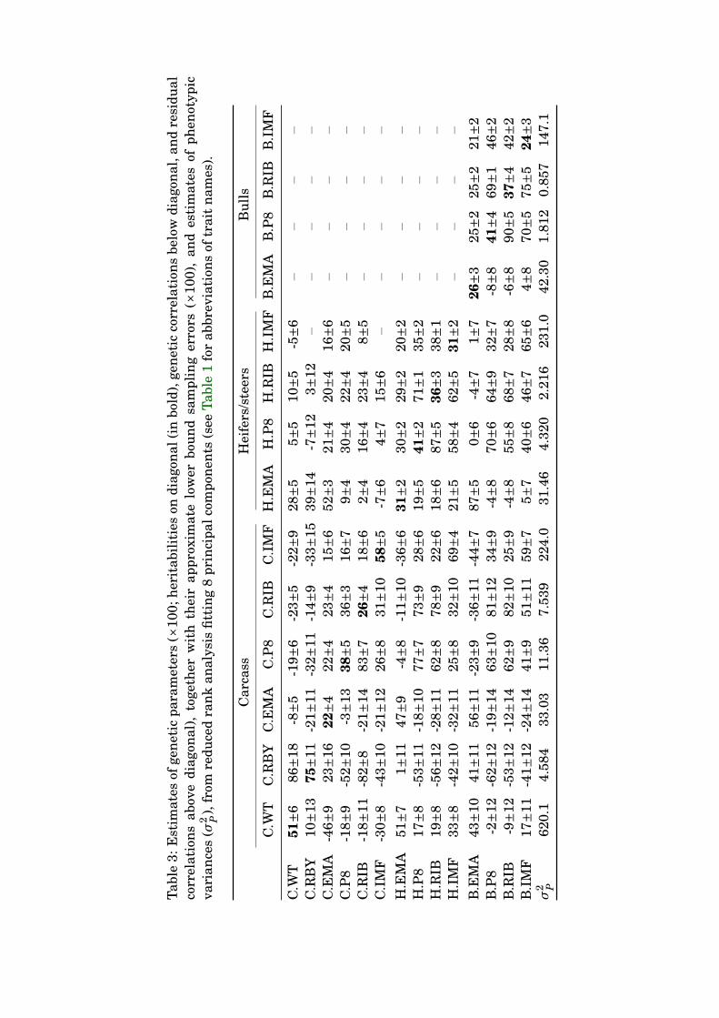
3.2 Estimates of variances and genetic parameters262

Changes in estimated genetic variances and heritabilities with increasing number of PCs263

(or factors) are displayed in Figure 3, together with estimates of their approximate lower264

bound sampling errors. Trends in estimates closely correspond to those in the estimates265

of genetic eigenvalues shown in Figure 1. Underestimates of eigenvalues and the total266

11


genetic variance when fitting too few PCs in reduced rank analyses are reflected in low267

estimates of variances and heritabilities, which gradually increase with the number of PCs268

considered. We expect a reduction in sampling variances when estimating less parameters.269

There is some indication of approximate sampling errors to increase from analyses F8 to270

F14 – where estimates have essentially reached a stable value – but effects are small and271

not completely consistent.272

The effect of the number of PCs considered on estimates of genetic correlations is illus-273

trated in Figure 4 for the three intra-muscular fat measures. If only one PC was fitted,274

all correlations would be forced a have an absolute value of unity. Fitting more and more275

PCs attenuates the correlations until they reach stable values. Hence, a considerable pro-276

portion of correlation estimates from analysis F4 were reduced in magnitude when fitting277

more PCs. As emphasized by the average squared deviation in correlations given in Ta-278

ble 1, there was little difference in estimates betwen analyses fitting 8 or more PCs.279

This is further illustrated in Figure 5, which contrasts estimates from analyses F8 and280

F14 for all genetic correlations and heritabilities and their approximate sampling errors.281

On the whole, there was close correspondence between estimates of parameters between282

the two analyses, with the largest difference for the correlation between C.IMF and B.IMF,283

which decreased from 0.59±0.11 (F8) to 0.46±0.18 (F14). Considering only 8 rather than284

all 14 PCs, estimates of sampling errors overall were reduced only by 0.01. However, as285

Figure 5 shows, values for the carcass traits tended to be lower for analysis F8, with a286

mean reduction of 0.02 and the maximum value of 0.09 for the estimate of the correlation287

between C.RBY and B.IMF, which was −0.41±0.11 and −0.52±0.20 for analyses F8 and288

F14, respectively. On the other hand, estimated sampling errors for some parameters were289

slightly increased for analysis F8. In part, this was explicable by an increase in magnitude.290

In addition, it should be borne in mind that values are estimates, based on large sample291

theory, and have been derived using linear approximations of non-linear functions (see292

Section A). Hence, some error in estimation is plausible.293

All estimates from analysis F8, together with their approximate sampling errors and es-294

timates of the phenotypic variance are summarised in Table 2. On the whole, estimates295

showed reasonable agreement with the results of Reverter et al. (2000) and previous esti-296

12


mates for scan traits based on about twice as much data for these traits (Meyer, 2005a).297

Obviously, with small numbers of records for the carcass traits, substantial fluctuations298

can occur when adding additional data, such as the progeny test records for C.WT, C.P8299

and C.RIB, altering the strategy to select data or changing the procedure of analysis. While300

some of the extreme estimates of Reverter et al. (2000) were moderated, others remained301

more or less unchanged. For instance, our estimates of genetic correlations between car-302

cass and heifer fat depths ranged from 0.6 to 0.8 while Reverter et al. (2000) reported303

values from 0.9 to unity. As fatness traits and EMA generally show little genetic associ-304

ation, our estimate of −0.24±0.14 for the genetic correlation between C.EMA and B.IMF305

seems more plausible than the value of −0.90±0.08 obtained in the former study. Notably,306

however, the estimated heritability for C.RBY remained very high (0.75±0.11 versus 0.68307

previously), and the estimate of a strong residual correlation with C.WT (0.86±0.18) was308

unchanged. Differences in heritability estimates for scan traits reported on different sexes309

were smaller than reported previously (Meyer and Graser, 1999; Meyer, 2005a). In partic-310

ular, heritabilities for fatness traits recorded on bulls were higher, which could be due to311

better than average recording practices in the small number of herds selected.312

3.3 Accuracy of genetic evaluation313

Table 4 shows the expected accuracy of genetic evaluation when considering reduced num-314

bers of principal components, for the example of a sire with 20 offspring of each sex with315

records for all 4 scan traits and 5 offspring with records for the 6 carcass traits. Values316

assuming estimates of covariances from the full rank analysis (F14) and from the reduced317

rank analysis with the lowest AICC (F8) are given. Mean accuracies from the simula-318

tion study agreed closely with expected values derived from the mixed model equations,319

differences being at most 0.02 except for index 2 where expected values were up to 0.06320

higher, and thus have been omitted. Similarly, results for 11, 12 and 13 PCs were virtually321

identical to those for 10 PCs, and are not shown.322

Values for individual carcass traits clearly reflect the weighting these receive in successive323

principal components. For instance, most information on C.WT, the trait with the highest324

variance, is supplied by the first PC, so that the accuracy of the corresponding EBV based325

13


only on PC1 is about 90% of that achieved when considering all PCs. Conversely, EBVs326

for C.EMA with low weightings in the first two PCs, did not achieve a reasonable accuracy327

until at least three PCs were taken into account. Only for C.RIB and C.P8 did it appear328

advantageous to fit more than 7 PCs.329

Most selection schemes consider a weighted combination of EBVs for individual traits.330

Hence, the effect of the number of PCs on sampling covariances as well as variances needs331

to be taken into account. This can be assessed by examining accuracies of indexes. Index332

1 comprised C.RBY, C.IMF, C.P8 and C.EMA with relative weights of 1, 2.661, 0.060, and333

−0.072, respectively, while Index 2 weighted C.RBY C.EMA and C.P8 in a ratio of 1 to 0.354334

to 0.208. These might represent indexes to select for an export market where high marbling335

is desirable and the domestic market (Barwick 2006; pers. comm.). Results suggest that,336

at the current estimates, at least 7 PCs need to be fitted so as not to compromise genetic337

progress.338

4 Discussion339

Results show that the genetic dispersion structure among the 14 carcass traits considered340

can be modelled parsimoniously by considering a subset of the genetic principal compo-341

nents. In contrast to other models which achieve parsimony by forcing estimates of covari-342

ance matrices to have a certain structure, no prior assumptions on the nature of covari-343

ances between variables are required. Whether a reduced rank of factor-analytic model344

is preferable depends on the circumstances. Both involve virtually the same calculations,345

relying on the identification of the leading PCs of a covariance matrix. Principal com-346

ponent analysis as such is merely concerned with identification of independent variables347

explaining the maximum amount of variation. In contrast, the underlying concept of factor348

analysis is to find the factors which explain the covariances between traits. This involves349

fitting a latent variable model with error variances equal to the specific variances. Thus,350

our reduced rank or ‘principal component’ analyses are equivalent to analyses fitting FA351

models where all specific variances are assumed to be zero.352

Allowing for non-zero specific variances in modelling the genetic covariance matrix re-353

14


duces the bias in estimates of the residual components when too few factors are considered.354

Hence, FA models tend to fit the data better than reduced rank models, in particular for355

small numbers of PCs, resulting in highly parsimonious models. The resulting estimates356

of covariance matrices are generally of full rank. Hence, FA models appear preferable to357

reduced rank analyses when our main objective is estimation of the covariance structure.358

Estimates from analyses assuming specific variances are zero have rank equal to the num-359

ber of factors fitted. Here, the assumption is that all important variation is captured by the360

subset of factors (or PCs) considered. This results in a set of mixed model equations of size361

proportional to the number of PCs rather than the number of traits. As computational re-362

quirements in mixed model analyses generally increase quadratically with the number of363

equations, even a small reduction in the number of PCs fitted can have a dramatic impact364

on the efficiency of analyses; see Meyer (2005a) for an example.365

In determining the number of factors to be fitted, there is a trade-off between bias, when366

omitting important PCs, and sampling variance, when fitting additional PCs which explain367

negligible variation. Simulations showed good agreement between the orders of fit selected368

on the basis of minimum BIC and the models yielding estimates of the genetic covariance369

with the smallest mean square errors (Meyer, 2005a,b). Corresponding estimates of ge-370

netic correlations from analysis F8 and from models with lowest BIC, a FA model with371

only 2 factors overall or a reduced rank model fitting 5 PCs when considering the latter372

models only, by and large had overlapping confidence regions. However, consistent and373

fairly substantial underestimates of the total genetic variation (see Table 2) and of genetic374

variances for individual traits (see Figure 3) were a concern. Hence, a conservative choice375

of ‘best’ model was made on the basis of AICC, which suggested that 8 PCs or 84 parame-376

ters were required to model the genetic covariance structure among the 14 traits. Selection377

index calculations indicated that the first 7 of these 8 PCs sufficed to account for genetic378

differences between animals in a genetic evaluation scheme. This implies that by adopting379

a parameterisation to estimate the leading genetic PC directly, the number of effects in a380

mixed model analysis of the 14 carcass traits could be halved.381

Individual estimates of genetic parameters were generally consistent with previous and382

literature results. Estimated sampling errors for correlations among carcass traits and383

correlations between carcass and scan traits, however, were fairly substantial. Clearly,384

15


more data for the carcass traits per se is required to obtain accurate estimates of their385

genetic relationships with the scan traits, and thus to ensure reliable estimates of breeding386

values based on these auxiliary traits.387

5 Conclusions388

Multivariate analyses fitting factor-analytic models for genetic covariance matrices are389

appealing, and can yield parsimonious models and more accurate estimates of genetic pa-390

rameters than ‘standard’ analyses considering matrices to be unstructured. Assuming391

specific variances to be zero gives reduced rank estimates which can be used to estimate392

the leading principal only, resulting in a dimension reduction and associated decrease in393

computational requirements of mixed model analyses.394

Acknowledgments395

This work was supported by grant BFGEN.100B of Meat and Livestock Australia Ltd396

(MLA).397

16


References398

Burnham, K. P., Anderson, D. R. (2004) Multimodel inference : Understanding AIC and399

BIC in model selection. Sociol. Meth. Res. 33:261–304. doi: 10.1177/0049124104268644.400

Graser, H. U., Tier, B., Johnston, D. J., Barwick, S. A. (2005) Genetic evaluation for the beef401

industry in Australia. Austr. J. Exp. Agric. 45. doi: 10.1071/EA05075.402

Henderson, C. R. (1975) Best linear unbiased estimation and prediction under a selection403

model. Biometrics 31:423–447.404

Kirkpatrick, M., Meyer, K. (2004) Simplified analysis of complex phenotypes : Direct es-405

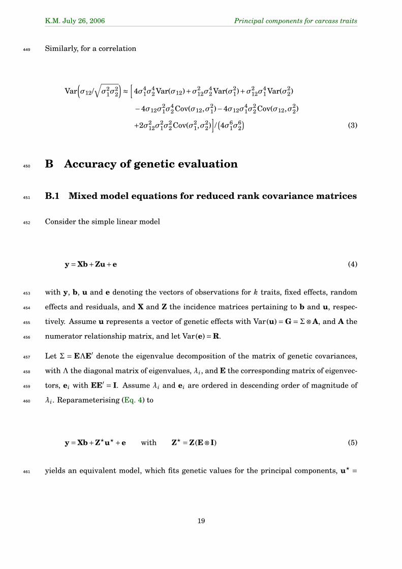
timation of genetic principal components. Genetics 168:2295–2306. doi: 10.1534/genet-406

ics.104.029181.407

Meyer, K. (2005a) Genetic principal components for live ultra-sound scan traits of Angus408

cattle. Anim. Sci. 81:337–345.409

Meyer, K. (2005b) Sampling behaviour of reduced rank estimates of genetic covariance410

functions. Proc. Ass. Advan. Anim. Breed. Genet. 16:286–289.411

Meyer, K. (2006a) PX x AI : algorithmics for better convergence in restricted maximum412

likelihood estimation. CD-ROM Eighth World Congr. Genet. Appl. Livest. Prod. Commu-413

nication No. 24–15.414

Meyer, K. (2006b) “WOMBAT” – digging deep for quantitative genetic analyses using re-415

stricted maximum likelihood. CD-ROM Eighth World Congr. Genet. Appl. Livest. Prod.416

Communication No. 27–14.417

Meyer, K., Graser, H. U. (1999) Estimates of parameters for scan records of Australian beef418

cattle treating records on males and females as different traits. Proc. Ass. Advan. Anim.419

Breed. Genet. 13:385–388.420

Meyer, K., Kirkpatrick, M. (2005a) Restricted maximum likelihood estimation of genetic421

principal components and smoothed covariance matrices. Genet. Select. Evol. 37:1–30.422

doi: 10.1051/gse:2004034.423

Meyer, K., Kirkpatrick, M. (2005b) Up hill, down dale : quantitative genetics of curvaceous424

traits. Phil. Trans. R. Soc. B 360:1443–1455. doi: 10.1098/rstb.2005.1681.425

Reverter, A., Johnston, D. J., Graser, H.-U., Wolcott, M. L., Upton, W. H. (2000) Genetic426

analyses of live-animal ultrasound and abattoir carcass traits in Australian Angus and427

Hereford cattle. J. Anim. Sci. 78:1786–1795.428

Thompson, R., Cullis, B. R., Smith, A. B., Gilmour, A. R. (2003) A sparse implementation of429

the Average Information algorithm for factor analytic and reduced rank variance models.430

Austr. New Zeal. J. Stat. 45:445–459. doi: 10.1111/1467-842X.00297.431

Wolfinger, R. D. (1993) Covariance structure selection in general mixed models. Comm.432

Stat. - Simul. Comp. 22:1079–1106.433

17

http://dx.doi.org/10.1177/0049124104268644

http://dx.doi.org/10.1071/EA05075

http://dx.doi.org/10.1534/genetics.104.029181



http://dx.doi.org/10.1051/gse:2004034

http://dx.doi.org/10.1098/rstb.2005.1681

http://dx.doi.org/10.1111/1467-842X.00297


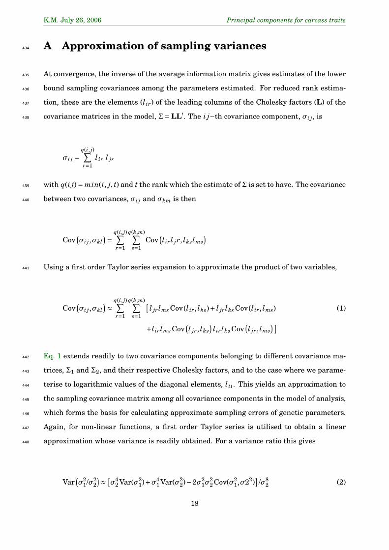
A Approximation of sampling variances434

At convergence, the inverse of the average information matrix gives estimates of the lower435

bound sampling covariances among the parameters estimated. For reduced rank estima-436

tion, these are the elements (l ir) of the leading columns of the Cholesky factors (L) of the437

covariance matrices in the model, Σ=LL′. The i j−th covariance component, σi j, is438

σi j =q(i, j)∑r=1

l ir l jr

with q(i j)= min(i, j, t) and t the rank which the estimate of Σ is set to have. The covariance439

between two covariances, σi j and σkm is then440

Cov(σi j,σkl

)= q(i, j)∑r=1

q(k,m)∑s=1

Cov(l ir l jr, lkslms

)Using a first order Taylor series expansion to approximate the product of two variables,441

Cov(σi j,σkl

)≈ q(i, j)∑r=1

q(k,m)∑s=1

[l jr lms Cov(l ir, lks)+ l jr lks Cov(l ir, lms) (1)

+l ir lms Cov(l jr, lks

)l ir lks Cov

(l jr, lms

)]Eq. 1 extends readily to two covariance components belonging to different covariance ma-442

trices, Σ1 and Σ2, and their respective Cholesky factors, and to the case where we parame-443

terise to logarithmic values of the diagonal elements, l ii. This yields an approximation to444

the sampling covariance matrix among all covariance components in the model of analysis,445

which forms the basis for calculating approximate sampling errors of genetic parameters.446

Again, for non-linear functions, a first order Taylor series is utilised to obtain a linear447

approximation whose variance is readily obtained. For a variance ratio this gives448

Var(σ2

1/σ22)≈ [

σ42 Var(σ2

1)+σ41 Var(σ2

2)−2σ21σ

22 Cov(σ2

1,σ22)]/σ8

2 (2)

18


Similarly, for a correlation449

Var(σ12/

√σ2

1σ22

)≈

[4σ4

1σ42 Var(σ12)+σ2

12σ42 Var(σ2

1)+σ212σ

41 Var(σ2

2)

−4σ12σ21σ

42 Cov(σ12,σ2

1)−4σ12σ41σ

22 Cov(σ12,σ2

2)

+2σ212σ

21σ

22 Cov(σ2

1,σ22)

]/(4σ6

1σ62)

(3)

B Accuracy of genetic evaluation450

B.1 Mixed model equations for reduced rank covariance matrices451

Consider the simple linear model452

y=Xb+Zu+e (4)

with y, b, u and e denoting the vectors of observations for k traits, fixed effects, random453

effects and residuals, and X and Z the incidence matrices pertaining to b and u, respec-454

tively. Assume u represents a vector of genetic effects with Var(u) = G = Σ⊗A, and A the455

numerator relationship matrix, and let Var(e)=R.456

Let Σ = EΛE′ denote the eigenvalue decomposition of the matrix of genetic covariances,457

with Λ the diagonal matrix of eigenvalues, λi, and E the corresponding matrix of eigenvec-458

tors, ei with EE′ = I. Assume λi and ei are ordered in descending order of magnitude of459

λi. Reparameterising (Eq. 4) to460

y=Xb+Z?u?+e with Z? =Z (E⊗I) (5)

yields an equivalent model, which fits genetic values for the principal components, u? =461

19


(E′⊗I

), instead of the original traits. The mixed model equations for (Eq. 5) are462

X′R−1X X′R−1Z?

Z?′R−1X Z?′R−1Z?+Λ−1 ⊗A−1

b

u?

= X′R−1y

Z?′R−1y

(6)

To consider only the leading m genetic principal components, replace E with Em, the k×m463

matrix comprising the first m columns of E, e1, . . ., em. This gives Z? with number of464

columns proportional to m rather than k. The number of equations in (Eq. 6) is reduced cor-465

respondingly (replacing Λ by its submatrix Λm consisting of the first m rows and columns),466

and u? contains m elements for each individual (Kirkpatrick and Meyer, 2004; Meyer and467

Kirkpatrick, 2005a). Genetic values for the k original traits can be obtained as simple468

linear combinations of the m genetic principal components,469

u= (Em ⊗I) u? (7)

Assuming that Σm = EmΛmE′m is the true genetic variance matrix, i.e. that λm+1, . . . ,λk470

are zero,471

Var(u?

)=Cov(u?,u?

)=Λm ⊗A−C (8)

Var(u)=Cov(u,u)=Σm ⊗A− (Em ⊗I)C(E′

m ⊗I)

(9)

where C is the part of the inverse of the coefficient matrix in (Eq. 6) pertaining to u?.472

Alternatively, we may have n ≤ k principal components with non-zero variance, but may473

want to examine sampling (co)variances of u resulting from considering the first m < n474

components only. In this case, we need to distinguish between true genetic covariances,475

G=EnΛnE′n ⊗A, and assumed values, G=Σm ⊗A, as outlined below (Section B.2).476

B.2 True and assumed genetic covariances are different477

In genetic evaluation via Best Linear Unbiased Prediction (BLUP), it is generally assumed478

that the values of covariance components due to random effects and residuals are known,479

20

i.e. are the population values. Under this assumption (e.g. Henderson, 1975),480

Var(u)=Cov(u,u)=G−C and Var(u−u)=C (10)

where u denotes a vector of genetic values with Var(u) = G, u represents its best linear481

unbiased predictor, and C is the part of the inverse of the coefficient matrix in the mixed482

model equations pertaining to u. If G 6= G is used in setting up the coefficient matrix,483

following the derivations of Henderson (1975), (co)variances in (Eq. 10) become484

Var(u)=G−CG−1G+ (I−CG−1)(I−GG−1)C (11)

Cov(u,u)=G−CG−1G (12)

Var(u−u)=C+C(I− G−1G

)G−1C (13)

Table 1: Characteristics of the data for traits measured on the carcass (C.WT : weight,C.EMA : eye muscle area, C.P8 : rump fat, C.RIB : rib fat, C.IMF : intra-muscular fat,and C.RBY : retail beef yield), and measured on live heifers or steers (H.EMA : eye musclearea, H.P8 rump fat, H.RIB rib fat, and H.IMF intra-muscular fat) and live bulls (B.EMA: eye muscle area, B.P8 : rump fat, B.RIB : rib fat, and B.IMF : intra-muscular fat).

Trait Number Mean Standard Mini- Maxi- Mean age Numberof records deviation mum mum (days) of CGa

C.WT (kg) 3 780 348.9 82.8 157 518 696.9 305C.RBY (%) 883 67.0 3.7 54 76 – 145C.EMA (cm2) 1 847 63.4 10.3 34 110 – 232C.P8 (mm) 3 385 15.34 8.57 1 36 – 291C.RIB (mm) 2 640 9.77 4.94 1 29 – 273C.IMF (%×10) 1 490 47.8 20.0 12 127 – 234H.EMA (cm2) 18 170 59.1 9.1 27 97 508.2 478H.P8 (mm) 18 362 6.34 3.15 1 25 507.5 481H.RIB (mm) 18 278 4.88 2.36 1 20 507.1 482H.IMF (%×10) 14 276 45.2 20.3 2 86 519.4 333B.EMA (cm2) 10 409 73.6 11.9 30 115 468.6 399B.P8 (mm) 10 313 3.79 1.81 1 21 469.0 395B.RIB (mm) 10 405 3.06 1.44 1 19 468.7 399B.IMF (%×10) 7 686 25.3 16.2 1 82 474.0 284

acontemporary groups

Table 2: Number of parameters (p) for different analyses (Fn : analysis fitting the leadingn principal components, Fn+ : analysis fitting a factor-analytic model with n factors), to-gether with the maximum log likelihood (logL ) values and Akaike (AICC) and Bayesian(BIC) information criteria (all scaled as deviation from the respective ‘best’ values), esti-mates of the total variation (

∑iλi) and measures of discrepancy to estimates from analysis

F14 (p∆r : square root of the average squared deviation of correlations, αi : angle between

estimates of the i−th eigenvectors).

p logL -½AICC -½BIC genetic residual∑iλi

p∆r α1 α2 α3

∑iλi

p∆r

F3 102 -407.3 -357.3 -244.7 386.6 0.273 37.3 37.0 61.2 953.3 0.044F4 113 -152.4 -113.5 -54.0 402.8 0.227 39.7 40.1 47.8 937.5 0.043F5 123 -82.2 -53.2 -42.1 471.3 0.190 29.0 28.9 70.4 874.3 0.054F6 132 -30.2 -10.3 -42.7 566.6 0.093 4.0 3.8 23.1 792.5 0.045F7 140 -14.0 -2.0 -73.1 588.2 0.068 1.7 2.0 20.6 772.9 0.020F8 147 -4.9 0 -104.9 593.1 0.035 0.8 1.5 23.6 768.2 0.009F9 153 -0.6 -1.7 -135.6 594.8 0.010 0.8 0.8 3.2 765.7 0.004F10 158 -0.1 -6.2 -164.3 592.9 0.005 0.2 0.2 1.1 767.0 0.001F11 162 0.0 -10.1 -187.5 592.6 0.001 0.1 0.1 0.7 767.2 0.000F14 168 -0.0 -16.2 -222.5 590.6 0 0 0 0 768.7 0F1+ 91 -276.7 -215.7 -49.9 440.7 0.232 89.3 0.0 0.0 886.2 0.054F2+ 104 -150.9 -103.0 0 494.1 0.183 18.4 27.5 0.0 843.6 0.043F3+ 116 -98.6 -62.6 -17.6 538.0 0.134 26.6 29.7 35.7 807.0 0.038F4+ 127 -53.8 -28.8 -37.1 546.0 0.117 30.9 31.9 22.1 805.2 0.046F5+ 137 -24.0 -9.1 -65.6 589.1 0.085 7.1 6.5 10.8 770.5 0.027F6+ 146 -10.6 -4.7 -104.7 597.0 0.046 1.2 1.7 12.1 764.6 0.022

Tabl

e3:

Est

imat

esof

gene

tic

para

met

ers

(×10

0;he

rita

bilit

ies

ondi

agon

al(i

nbo

ld),

gene

tic

corr

elat

ions

belo

wdi

agon

al,a

ndre

sidu

alco

rrel

atio

nsab

ove

diag

onal

),to

geth

erw

ith

thei

rap

prox

imat

elo

wer

boun

dsa

mpl

ing

erro

rs(×

100)

,an

des

tim

ates

ofph

enot

ypic

vari

ance

s(σ

2 P),

from

redu

ced

rank

anal

ysis

fitti

ng8

prin

cipa

lcom

pone

nts

(see

Tabl

e1

for

abbr

evia

tion

sof

trai

tna

mes

).

Car

cass

Hei

fers

/ste

ers

Bul

ls

C.W

TC

.RB

YC

.EM

AC

.P8

C.R

IBC

.IM

FH

.EM

AH

.P8

H.R

IBH

.IM

FB

.EM

AB

.P8

B.R

IBB

.IM

F

C.W

T51

±686

±18

-8±5

-19±

6-2

3±5

-22±

928

±55±

510

±5-5±6

––

––

C.R

BY

10±1

375

±11

-21±

11-3

2±11

-14±

9-3

3±15

39±1

4-7±1

23±

12–

––

––

C.E

MA

-46±

923

±16

22±4

22±4

23±4

15±6

52±3

21±4

20±4

16±6

––

––

C.P

8-1

8±9

-52±

10-3±1

338

±536

±316

±79±

430

±422

±420

±5–

––

–C

.RIB

-18±

11-8

2±8

-21±

1483

±726

±418

±62±

416

±423

±48±

5–

––

–C

.IM

F-3

0±8

-43±

10-2

1±12

26±8

31±1

058

±5-7±6

4±7

15±6

––

––

–H

.EM

A51

±71±

1147

±9-4±8

-11±

10-3

6±6

31±2

30±2

29±2

20±2

––

––

H.P

817

±8-5

3±11

-18±

1077

±773

±928

±619

±541

±271

±135

±2–

––

–H

.RIB

19±8

-56±

12-2

8±11

62±8

78±9

22±6

18±6

87±5

36±3

38±1

––

––

H.I

MF

33±8

-42±

10-3

2±11

25±8

32±1

069

±421

±558

±462

±531

±2–

––

–B

.EM

A43

±10

41±1

156

±11

-23±

9-3

6±11

-44±

787

±50±

6-4±7

1±7

26±3

25±2

25±2

21±2

B.P

8-2±1

2-6

2±12

-19±

1463

±10

81±1

234

±9-4±8

70±6

64±9

32±7

-8±8

41±4

69±1

46±2

B.R

IB-9±1

2-5

3±12

-12±

1462

±982

±10

25±9

-4±8

55±8

68±7

28±8

-6±8

90±5

37±4

42±2

B.I

MF

17±1

1-4

1±12

-24±

1441

±951

±11

59±7

5±7

40±6

46±7

65±6

4±8

70±5

75±5

24±3

σ2 P

620.

14.

584

33.0

311

.36

7.53

922

4.0

31.4

64.

320

2.21

623

1.0

42.3

01.

812

0.85

714

7.1

Table 4: Accuracy of genetic evaluation (E : expected value, se : empirical standard devi-ation from simulation) for carcass traits (see Table 1 for abbreviations) and two selectionindexes( IND1 and IND2) for a sire with 20 male and female progeny with records for the4 live scan traits each and 5 progeny with records for the 6 carcass traits, considering in-creasing numbers of genetic principal components and assuming estimates from analysisF14 or F8 are the population values.

No. PCs 1 2 3 4 5 6 7 8 9 10 14

Full rank analysis (F14)C.WT E 66.76 67.09 68.10 72.82 72.82 72.86 73.25 73.27 73.34 73.35 73.35

se 1.23 1.22 1.20 1.05 1.05 1.05 1.04 1.04 1.04 1.04 1.04C.RBY E 5.01 64.04 70.34 70.75 73.03 72.40 81.66 82.00 82.46 82.53 82.54

se 2.22 1.31 1.12 1.11 1.03 1.05 0.74 0.73 0.72 0.71 0.71C.EMA E 10.94 25.91 45.01 73.50 73.44 74.50 74.70 74.76 74.79 74.80 74.82

se 2.18 2.10 1.77 1.03 1.03 1.00 0.99 0.99 0.99 0.99 0.99C.IMF E 27.48 71.32 73.65 79.21 79.31 79.58 79.68 79.68 80.38 80.40 80.40

se 2.09 1.09 1.02 0.85 0.85 0.84 0.83 0.83 0.81 0.81 0.81C.P8 E 14.88 45.82 61.06 62.12 65.38 73.62 74.52 77.78 77.93 78.06 78.06

se 2.20 1.77 1.41 1.39 1.28 1.02 0.99 0.88 0.88 0.87 0.87C.RIB E 18.19 58.03 71.98 77.26 79.84 80.36 81.61 81.81 84.41 84.73 84.73

se 2.14 1.49 1.09 0.91 0.81 0.80 0.75 0.75 0.65 0.64 0.64IND1 E 24.63 26.32 47.04 62.75 67.66 68.19 72.92 73.12 75.30 75.30 75.30

se 2.10 2.05 1.74 1.36 1.21 1.19 1.04 1.04 0.96 0.96 0.96IND2 E 5.01 64.04 70.34 70.75 73.03 72.40 81.66 82.00 82.46 82.53 82.54

se 2.22 1.31 1.12 1.11 1.03 1.05 0.74 0.73 0.72 0.71 0.71Reduced rank analysis (F8)

C.WT E 67.63 68.27 71.08 73.60 73.61 73.55 74.14 74.16se 1.22 1.20 1.12 1.03 1.03 1.04 1.02 1.02

C.RBY E 6.49 57.09 59.97 62.34 70.23 71.32 82.21 82.49se 2.24 1.51 1.43 1.37 1.12 1.09 0.72 0.71

C.EMA E 11.69 22.62 59.73 73.06 73.59 74.33 74.49 74.58se 2.23 2.13 1.46 1.05 1.03 1.01 1.00 1.00

C.IMF E 27.82 76.63 76.07 82.51 84.06 84.22 84.29 84.29se 2.06 0.93 0.95 0.71 0.66 0.65 0.65 0.65

C.P8 E 16.06 45.74 62.33 67.27 71.51 73.33 76.57 80.28se 2.15 1.77 1.36 1.23 1.10 1.03 0.92 0.79

C.RIB E 19.31 58.38 71.69 82.68 87.78 87.67 88.26 88.67se 2.14 1.48 1.09 0.70 0.51 0.51 0.49 0.47

IND1 E 24.26 38.72 39.31 62.47 76.04 75.65 80.93 81.13se 2.11 1.92 1.91 1.36 0.95 0.96 0.78 0.77

IND2 E 6.49 57.09 59.97 62.34 70.23 71.32 82.21 82.49se 2.26 1.53 1.46 1.40 1.15 1.09 0.72 0.72

Figure 1: Estimates of the first 6 eigenvalues of genetic (•), residual (N) and phenotypic (�)covariance matrices from a full rank, multivariate analyses (F14), reduced rank analysesfitting increasing numbers of genetic principal components (F3 to F11) and analyses fittinga factor-analytic structure for the genetic covariance matrix with increasing numbers (F1+to F6+) of factors (Horizontal lines indicate values for analysis F14).

●

●

●●

● ●

● ●

●

●● ● ● ● ● ●

First

200

400

600

● ●

●

●

●●

●●

●

● ● ●● ● ● ●

Second

100

150

200

250

300

●●

●●

●●

● ●● ● ● ●

● ● ● ●

Third

050

100

150

200

● ●

●● ● ●

●●

● ● ● ● ● ● ●

Fourth

050

100

150

F1+

F2+

F3+

F4+

F5+

F6+ F

3

F4

F5

F6

F7

F8

F9

F10

F11

F14

● ●● ●

●

●

●

●● ● ● ● ● ●

Fifth

010

2030

4050

60

F1+

F2+

F3+

F4+

F5+

F6+ F

3

F4

F5

F6

F7

F8

F9

F10

F11

F14

●

●● ● ● ●

● ● ●

● ● ● ●

Sixth

010

2030

40

Figure 2: Estimates of weights for individual traits (see Table 1 for abbreviations) in thefirst 6 genetic principal components from a reduced rank analysis fitting 8 principal com-ponents (• : as estimated, and ◦ : divided by estimated genetic standard deviation andscaled by 6 for first and second and scaled by 3 otherwise), and a full rank analysis (×).

First

●

●

●

● ●

●●

●●●

●●

● ●

●

●●

● ●● ● ●● ● ●

●

●●

−.8

−.4

0

0.4

0.8

Second

●

● ●●

●

●● ●● ● ●

● ●●

●

● ● ● ●● ● ●● ● ●

●

●

●

Third

● ●

● ● ●

● ● ●●●

●

●

●●

●

●

●● ●

● ● ●● ● ●

●

●●

−.8

−.4

0

0.4

0.8

Fourth

●

●● ●

●

●

●

●●

●

●

●●

●

●●

● ●●

●

●●●

●●

●

●

●

C.W

T

C.R

BY

C.E

MA

C.P

8

C.R

IB

C.IM

F

H.E

MA

H.P

8

H.R

IB

H.IM

F

B.E

MA

B.P

8

B.R

IB

B.IM

F

Fifth

●

●

●

●

●

● ●

●

● ●

●

●

●

●●

●●

●

●

●●

●

●●

●

●

●

●

−.8

−.4

0

0.4

0.8

C.W

T

C.R

BY

C.E

MA

C.P

8

C.R

IB

C.IM

F

H.E

MA

H.P

8

H.R

IB

H.IM

F

B.E

MA

B.P

8

B.R

IB

B.IM

FSixth

●

●

●●

●

●

● ●●

●

●

●

●●

●

●

●

●

●

●

● ●●

●●

●

●

●

Figure 3: Estimates of genetic variances (•) and heritabilities (�) for selected traits (seeTable 1 for definition of abbreviations), together with their approximate lower bound sam-pling errors, from reduced rank analyses fitting increasing numbers of principal compo-nents (F3 to F11), a standard multivariate analysis (F14) and analyses fitting a factor-analytic model (F1+ to F6+).

5010

015

020

0

●

●●

● ● ● ● ● ● ●

●● ●

●●

●

C.IMF

5560

6570

7580

●●

● ● ● ● ● ● ● ●

●

● ●●

●

●

H.IMF

24

68

10

● ●

●

●

● ● ● ● ● ●

●

●

●

●

●

●

C.EMA

150

250

350

● ●

●

●● ● ● ● ● ●

●

●

●●

● ●

C.WT

12

34

5

●●

●

●

●

●● ● ● ●

● ● ● ● ● ●

C.RBY

2.5

3.0

3.5

4.0

4.5

5.0

●● ●

●

●

●● ● ● ●

●●

● ●● ●

C.P8

F1+

F2+

F3+

F4+

F5+

F6+ F

3F

4F

5F

6F

7F

8F

9F

10F

11F

14

0.2

0.3

0.4

0.5

0.6 C.WT

F1+

F2+

F3+

F4+

F5+

F6+ F

3F

4F

5F

6F

7F

8F

9F

10F

11F

14

0.3

0.5

0.7

0.9

C.RBY

F1+

F2+

F3+

F4+

F5+

F6+ F

3F

4F

5F

6F

7F

8F

9F

10F

11F

14

0.1

0.2

0.3

0.4

0.5 C.P8

Figure 4: Estimates of genetic correlations for intra-muscular fat content measured on thecarcass (left), on live heifers and steers (middle) or bulls (right) with all other traits (seeTable 1 for abbreviations), from analyses fitting 4 (H), 6 (•), 8 (N), and all 14 (�) geneticprincipal components.

−1

−.5

0

0.5

1

●●

●

●●

●

●

● ●

●

●

●●

●

Carcass

−1

−.5

0

0.5

1

●

●●

●

●

●

●

● ●

●

●

●●

●

Heifers

C.W

T

C.R

BY

C.E

MA

C.P

8

C.R

IB

C.IM

F

H.E

MA

H.P

8

H.R

IB

H.IM

F

B.E

MA

B.P

8

B.R

IB

B.IM

F

−1

−.5

0

0.5

1

●

● ●

● ●●

●

● ●

●

●

● ●

●Bulls

Figure 5: Estimates of genetic parameter (•) and their approximate lower bound samplingerrors (�) from a full rank analysis (F14) and a reduced rank analysis fitting 8 principalcomponents (F8); closed symbols pertain to parameters among the live scan traits only,open symbols pertain to estimates involving carcass traits.

F14

F8

−1.

0

−0.

5

0.0

0.5

1.0

−1.

0−

0.5

0.0

0.5

1.0

●

●

●

●

●

●

●

●●

●

●●●

●

●

●●

●●

●

●

●●●

●

●

●

●

●

●

●

●

●

●

●

●●

●

●

●

●●

●

●

●

●

●

●

●●

●

●●

●

●

●

●

●

●●

●

●

●

●

●●

●●

●

●●

●

●

●

●●●

●

●

●

●

●●●

●

●

●

●

●

●

●●

●

●

●

●

●●

●

●

●

●●

●

●

F14

0.00

0.05

0.10

0.15

0.20

0.00

0.05

0.10

0.15

0.20

multivariate analyses of carcass traits for angus cattle...

Documents