multivariable calculus - james cook's · pdf filemultivariable calculus james s. cook...
TRANSCRIPT

Multivariable Calculus
James S. CookLiberty University
Department of Mathematics
Fall 2011

2
preface
how to succeed in calculus
I do use the textbook, however, I follow these notes. You should use both. From past experienceI can tell you that the students who excelled in my course were those students who both studiedmy notes and read the text. They also came to every class and paid attention. I recommend thefollowing course of study:
1. submit yourself to learn, keep a positive attitude. This course is a lot of work. Yes, probablymore than 3 others for most people. Most people have a lot of work to do in getting up tospeed on real mathematical thinking. There is no substitute for time and effort. If you’recomplaining in your mind about the workload etc... then you’re wasting your time.
2. come to class, take notes, think.
3. read these notes.
4. attempt Problem Sets, you will likely find forming a study group is essential for success here.I ask some very hard questions. The majority of the hwk grade comes from Problem Sets.
format of my notes
These notes were prepared with LATEX. You’ll notice a number of standard conventions in my notes:
1. definitions are usually in green.
2. remarks are in red.
3. theorems, propositions, lemmas and corollaries are in blue.
4. proofs start with a Proof: and are concluded with a �.
5. often figures in these notes were prepared with Graph, a simple and free math graphingprogram, or Maple, or Mathematica. Or some online math tool, of which there are dozens.
By now the abbreviations below should be old news, but to be safe I replicate them here once more:

3
Finally, please be warned these notes are a work in progress. I look forward to your input on howthey can be improved, corrected and supplemented. This is my second set of notes for calculus III.I follow approximately the same LATEXformat as I used for the Calculus I and II notes of 2010-2011.The old handwritten calculus III notes are not bad, but I want to improve the theoretical aspectsof these notes. I have included most of the examples from the old notes and also a myriad ofhomework solutions in this version. There are far too many examples for lecture. My goal was togather the examples in a convenient format for the student.
Please understand that the definitions given in these notes are primary. I recommendStewart for additional examples, but not for definitions in this course. These notes takea different (and I hope clearer) path through the subject matter of multivariable calculus, I make noeffort to be consistent with the text’s development of concepts and I intend to add much detail onhow calculus III works in curvelinear coordinates (not in Stewart). It is my intent these notes are aself-contained treatment of differential multivariate calculus. However, you should understand thatI do assume you have a complete and working knowledge of Calculus I and II, basically Chapters

4
1-12 of Stewart, or take a look at my website for a breakdown of Math 131-132 as offered at LibertyUniversity.
At this juncture there are about 285 pages. I would like to add another 50 pictures, but, I’ll savethem for class. These notes only cover the material for the first two tests. I will probably transitionto the old notes after that point. However, I have more work to do on the last half of the course soI would kindly ask you refrain from printing the old notes on integration and vector calculus. It ishighly likely that I am going to edit them and add discussion, proofs and totally new calculations.I will let you know when I have notes beyond those found here1
The old notes and much more can be found at my calculus III webpage. Every so often I mentionthe existence of an animation on my webpage. I am opening a zoo of gif-files where you can go seeall sorts of mathematical creatures. If you create interesting creatures I will (with your permission)happily add them to my collection.
James Cook, August 21, 2011.version 2.0
1of course, if you’ve got money to burn and/or you just want to offend Al Gore by wasteful printing then go forit, I always respect those who wish to make Al Gore cry.

Contents
1 analytic geometry 9
1.1 vectors in euclidean space . . . . . . . . . . . . . . . . . . . . . . . . . . . . . . . . . 10
1.2 the cross product . . . . . . . . . . . . . . . . . . . . . . . . . . . . . . . . . . . . . . 29
1.3 lines and planes in R 3 . . . . . . . . . . . . . . . . . . . . . . . . . . . . . . . . . . . 40
1.3.1 parametrized lines and planes . . . . . . . . . . . . . . . . . . . . . . . . . . . 40
1.3.2 lines and planes as solution sets . . . . . . . . . . . . . . . . . . . . . . . . . . 42
1.3.3 lines and planes as graphs . . . . . . . . . . . . . . . . . . . . . . . . . . . . . 46
1.3.4 on projections onto a plane . . . . . . . . . . . . . . . . . . . . . . . . . . . . 47
1.3.5 additional examples . . . . . . . . . . . . . . . . . . . . . . . . . . . . . . . . 50
1.4 curves . . . . . . . . . . . . . . . . . . . . . . . . . . . . . . . . . . . . . . . . . . . . 54
1.4.1 curves in two-dimensional space . . . . . . . . . . . . . . . . . . . . . . . . . . 54
1.4.2 how can we find the Cartesian form for a given parametric curve? . . . . . . 62
1.4.3 curves in three dimensional space . . . . . . . . . . . . . . . . . . . . . . . . . 67
1.5 surfaces . . . . . . . . . . . . . . . . . . . . . . . . . . . . . . . . . . . . . . . . . . . 70
1.5.1 surfaces as graphs . . . . . . . . . . . . . . . . . . . . . . . . . . . . . . . . . 70
1.5.2 parametrized surfaces . . . . . . . . . . . . . . . . . . . . . . . . . . . . . . . 72
1.5.3 surfaces as level sets . . . . . . . . . . . . . . . . . . . . . . . . . . . . . . . . 75
1.5.4 combined concept examples . . . . . . . . . . . . . . . . . . . . . . . . . . . . 81
1.6 curvelinear coordinates . . . . . . . . . . . . . . . . . . . . . . . . . . . . . . . . . . . 83
1.6.1 polar coordinates . . . . . . . . . . . . . . . . . . . . . . . . . . . . . . . . . . 83
1.6.2 cylindrical coordinates . . . . . . . . . . . . . . . . . . . . . . . . . . . . . . . 84
1.6.3 spherical coordinates . . . . . . . . . . . . . . . . . . . . . . . . . . . . . . . . 87
2 calculus and geometry of curves 91
2.1 calculus for curves . . . . . . . . . . . . . . . . . . . . . . . . . . . . . . . . . . . . . 91
2.2 geometry of smooth oriented curves . . . . . . . . . . . . . . . . . . . . . . . . . . . . 103
2.2.1 arclength . . . . . . . . . . . . . . . . . . . . . . . . . . . . . . . . . . . . . . 103
2.2.2 vector fields along a path . . . . . . . . . . . . . . . . . . . . . . . . . . . . . 107
2.2.3 Frenet Serret equations . . . . . . . . . . . . . . . . . . . . . . . . . . . . . . 110
2.2.4 curvature . . . . . . . . . . . . . . . . . . . . . . . . . . . . . . . . . . . . . . 116
2.2.5 osculating plane and circle . . . . . . . . . . . . . . . . . . . . . . . . . . . . . 119
2.3 physics of motion . . . . . . . . . . . . . . . . . . . . . . . . . . . . . . . . . . . . . . 122
5

6 CONTENTS
2.3.1 position vs. displacement vs. distance traveled . . . . . . . . . . . . . . . . . 125
3 multivariate limits 133
3.1 open sets . . . . . . . . . . . . . . . . . . . . . . . . . . . . . . . . . . . . . . . . . . 133
3.2 the multivariate limit and continuity . . . . . . . . . . . . . . . . . . . . . . . . . . . 135
3.3 multivariate indeterminants . . . . . . . . . . . . . . . . . . . . . . . . . . . . . . . . 142
3.3.1 additional examples . . . . . . . . . . . . . . . . . . . . . . . . . . . . . . . . 147
4 differentiation 149
4.1 directional derivatives . . . . . . . . . . . . . . . . . . . . . . . . . . . . . . . . . . . 150
4.2 partial differentiation in R 2 . . . . . . . . . . . . . . . . . . . . . . . . . . . . . . . . 153
4.2.1 directional derivatives and the gradient in R 2 . . . . . . . . . . . . . . . . . . 161
4.2.2 gradient vector fields . . . . . . . . . . . . . . . . . . . . . . . . . . . . . . . . 167
4.2.3 contour plots . . . . . . . . . . . . . . . . . . . . . . . . . . . . . . . . . . . . 171
4.3 partial differentiation in R 3 and Rn . . . . . . . . . . . . . . . . . . . . . . . . . . . . 175
4.3.1 directional derivatives and the gradient in R 3 and Rn . . . . . . . . . . . . . 179
4.3.2 gradient vector fields in R 3 and Rn . . . . . . . . . . . . . . . . . . . . . . . . 183
4.4 the general derivative . . . . . . . . . . . . . . . . . . . . . . . . . . . . . . . . . . . 188
4.4.1 matrix of the derivative . . . . . . . . . . . . . . . . . . . . . . . . . . . . . . 188
4.4.2 tangent space as graph of linearization . . . . . . . . . . . . . . . . . . . . . . 190
4.4.3 existence and connections to directional differentiation . . . . . . . . . . . . . 192
4.4.4 properties of the derivative . . . . . . . . . . . . . . . . . . . . . . . . . . . . 200
4.5 chain rules . . . . . . . . . . . . . . . . . . . . . . . . . . . . . . . . . . . . . . . . . . 203
4.6 tangent spaces and the normal vector field . . . . . . . . . . . . . . . . . . . . . . . . 218
4.6.1 level surfaces and tangent space . . . . . . . . . . . . . . . . . . . . . . . . . . 219
4.6.2 parametrized surfaces and tangent space . . . . . . . . . . . . . . . . . . . . . 220
4.6.3 tangent plane to a graph . . . . . . . . . . . . . . . . . . . . . . . . . . . . . . 223
4.7 partial differentiation with side conditions . . . . . . . . . . . . . . . . . . . . . . . . 226
4.8 gradients in curvelinear coordinates . . . . . . . . . . . . . . . . . . . . . . . . . . . . 238
4.8.1 polar coordinates . . . . . . . . . . . . . . . . . . . . . . . . . . . . . . . . . . 238
4.8.2 cylindrical coordinates . . . . . . . . . . . . . . . . . . . . . . . . . . . . . . . 239
4.8.3 spherical coordinates . . . . . . . . . . . . . . . . . . . . . . . . . . . . . . . . 239
5 optimization 243
5.1 lagrange multipliers . . . . . . . . . . . . . . . . . . . . . . . . . . . . . . . . . . . . 244
5.1.1 proof of the method . . . . . . . . . . . . . . . . . . . . . . . . . . . . . . . . 244
5.1.2 examples of the method . . . . . . . . . . . . . . . . . . . . . . . . . . . . . . 245
5.1.3 extreme values of a quadratic form on a circle . . . . . . . . . . . . . . . . . . 258
5.1.4 quadratic forms in n-variables* . . . . . . . . . . . . . . . . . . . . . . . . . . 262
5.2 multivariate taylor series . . . . . . . . . . . . . . . . . . . . . . . . . . . . . . . . . . 263
5.2.1 taylor’s polynomial for one-variable . . . . . . . . . . . . . . . . . . . . . . . . 263
5.2.2 taylor’s multinomial for two-variables . . . . . . . . . . . . . . . . . . . . . . 264
5.2.3 taylor’s multinomial for many-variables . . . . . . . . . . . . . . . . . . . . . 267

CONTENTS 7
5.3 critical point analysis . . . . . . . . . . . . . . . . . . . . . . . . . . . . . . . . . . . . 2705.3.1 a view towards higher dimensional critical points* . . . . . . . . . . . . . . . 277
5.4 closed set method . . . . . . . . . . . . . . . . . . . . . . . . . . . . . . . . . . . . . . 279
6 integration 285
7 vector calculus 287

8 CONTENTS
Chapter 1
analytic geometry
Euclidean space is named for the ancient mathematician Euclid. In Euclid’s view geometry wasa formal system with axioms and constructions. For example, the fact two parallel lines neverinterect is called the parallel postulate. If you take the course in modern geometry then you’ll studymore of the history of Euclid. Fortunately for us the axiomatic/constructive approach was replacedby a far easier view about 400 years ago. Rene Descartes made popular the idea of using numbersto label points in space. In this new Cartesian geometry the fact two parallel lines in a plane neverintersect could be checked by some simple algebraic calculation. More than this, all sorts of curves,surfaces and even more fantastic objects became constructible in terms of a few simple algebraicequations. The idea of using numbers to label points and the resulting geometry governed by theanalysis of those numbers is called analytic geometry. We study the basics of analytic geometryin this chapter.
In your previous mathematical studies you have already dealt with analytic geometry in the plane.Trigonometry provided a natural framework to decipher all sorts of interesting facts about trian-gles. Moreover, the study of trigonometric functions in turn has allowed us solutions to otherwiseintractable integrals in calculus II. Trigonometric substitution is an example of where the geometryof triangles has allowed deeper analysis. It goes both ways. Geometry inspires analysis and analysisunravels geometry. These are two sides of something deeper.
In this course we need to tackel three dimensional problems. The proper notation which groupstogether concepts in the most efficient and clean manner is the vector notation. Historically, it waspredated by the quaternionic analysis of Hamilton, but for about 120 year the vector notation hasbeen the dominant framework for two and three dimensional analytic geometry1. In particular,the dot and cross products allow us to test for how parallel two lines are, or to project a line ontoa plane, or even to calculate the direction which is perpendicular to a pair of given directions.Engineering and basic everyday physics all written in this vector langauge.
1general geometries are more naturally understood in the language of differential forms and manifolds, but this iswhere we all must begin
9

10 CHAPTER 1. ANALYTIC GEOMETRY
We also continue our study of functions in this chapter. We have studied functions f : U ⊆ R→ Rin the first two semesters of calculus. One goal in this course is to extend the analysis to functionsof many variables. For example, f : R 2 → R with f(x, y) = x2 + y2. What can we say aboutthis function? What calculus is known to analyze the properties of f? Before we begin to answersuch questions in future chapters, we need to spend some time on the basic geometry of Rn andthen especially R 3. Naturally, we use R 3 to model the three spatial dimensions which frame oureveryday existence2.
In this chapter we are concerned with understanding how to analytically describe points, curvesand surfaces. We will examine what the solution set of z = f(x, y) looks like for various f . Or,what is the solution set of F (x, y) = k, or F (x, y, z) = k? We learn how think about mappingst 7→ 〈x(t), y(t), z(t)〉 or (u, v) 7→ 〈x(u, v), y(u, v), z(u, v)〉. What is the geometry of such mappings?These are questions we hope to answer, at least in part, in this chapter.
1.1 vectors in euclidean space
We denote the real numbers as R = R1. Naturally R is identified with a line as we are taught in ourprevious study of the number line. The Cartesian products of R with itself give us natural modelsfor the plane, 3 dimensional space and more abstractly n-dimensional space:
Definition 1.1.1. .
1. two-dimensional space: is the set of all ordered pairs of real numbers:
R 2 = R× R = {(x, y) | x, y ∈ R}
2. three-dimensional space: is the set of all ordered triples of real numbers:
R 3 = R× R× R = {(x, y, z) | x, y, z ∈ R}
3. n-dimensional space: is the set of all n-tuples of real numbers:
Rn = R× R× · · · × R︸ ︷︷ ︸n copies
= {(x1, x2, . . . , xn) | xj ∈ R for each j ∈ Nn}
The fact that the n-tuples above are ordered means that two n-tuples are equal iff each and everyentry in the n-tuple matches.
2I would not say we live in R 3, it’s just a model, it’s not reality. Respectable philosophers as recently as 200years ago labored under the delusion that euclidean space must be reality since that was all they could imagine asreasonable

1.1. VECTORS IN EUCLIDEAN SPACE 11
Definition 1.1.2. vector equality, components.
In particular, (v1, v2, . . . , vn) = (w1, w2, . . . , wn) iff v1 = w1, v2 = w2, . . . , vn = wn. Inthe context of R 2 we say a is the x-component of (a, b) whereas b is the y-componentof (a, b). In the context of R 3 we say a is the x-component of (a, b, c) whereas b is they-component of (a, b, c) and c is the z-component of (a, b, c). Generally, we say vj thej-th component of (v1, v2, . . . , vn).
The sometimes the term euclidean is added to emphasize that we suppose distance between pointsis measured in the usual manner. Recall that in the one-dimensional case the distance betweenx, y ∈ R is given by the absolute value function; d(x, y) = |y− x| =
√(y − x)2. We define distance
in n-dimensions by similar formulas:
Definition 1.1.3. euclidean distance.
1. distance in two-dimensional euclidean space: if p1 = (x1, y1), p2 = (x2, y2) ∈ R 2
then the distance between points p1 and p2 is
d(p1, p2) =√
(x2 − x1)2 + (y2 − y1)2.
2. distance in three-dimensional euclidean space: if p1 = (x1, y1, z1), p2 =(x2, y2, z2) ∈ R 3 then the distance between points p1 and p2 is
d(p1, p2) =√
(x2 − x1)2 + (y2 − y1)2 + (z2 − z1)2.
3. distance in n-dimensional euclidean space: if a, b ∈ Rn where a = (a1, a2, . . . , an)and b = (b1, b2, . . . , bn) then the distance between points a and point b is
d(a, b) =
√√√√ n∑j=1
(bj − aj)2 =√
(b1 − a1)2 + (b1 − a1)2 + · · ·+ (bn − an)2.
It is simple to verify that the definition above squares with our traditional ideas about distance fromprevious math courses. In particular, notice these follow from the Pythagorean theorem applied toappropriate triangles. The picture below shows the three dimensional distance formula is consistentwith the two dimensional formula.

12 CHAPTER 1. ANALYTIC GEOMETRY
Notice that there is a natural correspondance between points and directed line-segments from theorigin. We can view an n-tuple p as either representing the point (p1, p2, . . . , pn) or the directedline-segment from the origin (0, 0, . . . , 0) to the point (p1, p2, . . . , pn).
We will use the notation ~p for n-tuples throughout the remainder of these notes to emphasize thefact that ~p is a vector. Some texts use bold to denote vectors, but I prefer the over-arrow notationwhich is easily duplicated in hand-written work. The directed line-segment from point P to pointQ is naturally identified with the vector ~P − ~Q as illustrated below:

1.1. VECTORS IN EUCLIDEAN SPACE 13
This is consistent with the identification of points and vectors based at the origin. See how thevector ~a and ~b are connected by the vector ~b− ~a
We add vectors geometrically by the tip-to-tail method as illustrated below.
Also, we rescale them by shrinking or stretching their length by a scalar multiple:

14 CHAPTER 1. ANALYTIC GEOMETRY
More pictures usually help:
In the diagram below we illustrate the geometry behind the vector equation
~R = ~A+ ~B + ~C + ~D.
Continuiing in this way we can add any finite number of vectors in the same tip-2-tail fashion.
1.1. VECTORS IN EUCLIDEAN SPACE 15
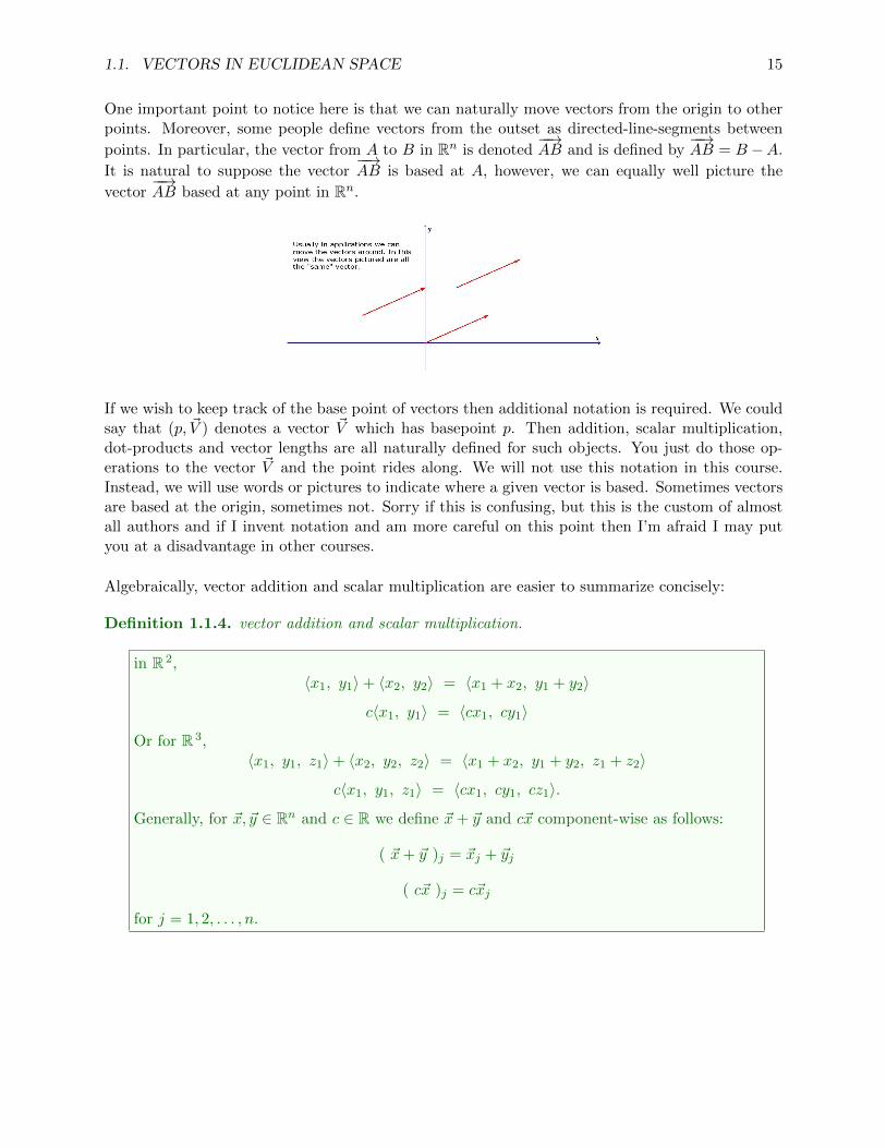
One important point to notice here is that we can naturally move vectors from the origin to otherpoints. Moreover, some people define vectors from the outset as directed-line-segments between
points. In particular, the vector from A to B in Rn is denoted−−→AB and is defined by
−−→AB = B −A.
It is natural to suppose the vector−−→AB is based at A, however, we can equally well picture the
vector−−→AB based at any point in Rn.
If we wish to keep track of the base point of vectors then additional notation is required. We couldsay that (p, ~V ) denotes a vector ~V which has basepoint p. Then addition, scalar multiplication,dot-products and vector lengths are all naturally defined for such objects. You just do those op-erations to the vector ~V and the point rides along. We will not use this notation in this course.Instead, we will use words or pictures to indicate where a given vector is based. Sometimes vectorsare based at the origin, sometimes not. Sorry if this is confusing, but this is the custom of almostall authors and if I invent notation and am more careful on this point then I’m afraid I may putyou at a disadvantage in other courses.
Algebraically, vector addition and scalar multiplication are easier to summarize concisely:
Definition 1.1.4. vector addition and scalar multiplication.
in R 2,〈x1, y1〉+ 〈x2, y2〉 = 〈x1 + x2, y1 + y2〉
c〈x1, y1〉 = 〈cx1, cy1〉
Or for R 3,〈x1, y1, z1〉+ 〈x2, y2, z2〉 = 〈x1 + x2, y1 + y2, z1 + z2〉
c〈x1, y1, z1〉 = 〈cx1, cy1, cz1〉.
Generally, for ~x, ~y ∈ Rn and c ∈ R we define ~x+ ~y and c~x component-wise as follows:
( ~x+ ~y )j = ~xj + ~yj
( c~x )j = c~xj
for j = 1, 2, . . . , n.

16 CHAPTER 1. ANALYTIC GEOMETRY
Given these definitions it is often convenient to break a vector down into its vector components.In particular, for R 2, define x = 〈1, 0〉 and y = 〈0, 1〉 hence:
〈a, b〉 = 〈a, 0〉+ 〈0, b〉= a〈1, 0〉+ b〈0, 1〉= a x+ b y (1.1)
Definition 1.1.5. vector and scalar components of two-vectors.
The vector component of 〈a, b〉 in the x-direction3 is simply a x whereas the vectorcomponent of 〈a, b〉 in the y-direction is simply b y. In contrast, a, b are the scalar com-ponents of 〈a, b〉 in the x, y-directions respective.
Scalar components are scalars whereas vector components are vectors. These are entirely differentobjects if n 6= 1, please keep clear this distinction in your mind. Notice that the vector componentsare what we use to reproduce a given vector by the tip-to-tail sum:
For R 3 we define the following notation: x = 〈1, 0, 0〉, y = 〈0, 1, 0〉, and z = 〈0, 0, 1〉 hence:
〈a, b, c〉 = 〈a, 0, 0〉+ 〈0, b, 0〉+ 〈0, 0, c〉= a〈1, 0, 0〉+ b〈0, 1, 0〉+ c〈0, 0, 1〉= a x+ b y + c z (1.2)
Definition 1.1.6. vector and scalar components of three-vectors.
The vector components of 〈a, b, c〉 are: a x in the x-direction4, b y in the y-direction andc z in the z-direction. In contrast, a, b, c are the scalar components of 〈a, b, c〉 in thex, y, z-directions respective.
Again, I emphasize that vector components are vectors whereas components or scalar componentsare by default scalars.

1.1. VECTORS IN EUCLIDEAN SPACE 17
The story for Rn is not much different. Define for j = 1, 2, . . . , n the vector xj = 〈0, 0, . . . , 1, . . . , 0〉where the 1 appears in the j-th entry, hence:
〈a1, a2, . . . , an〉 = 〈a1, 0, . . . , 0〉+ 〈0, a2, . . . , 0〉+ · · ·+ 〈0, 0, . . . , an〉= a1〈1, 0, . . . , 0〉+ a2〈0, 1, . . . , 0〉+ · · ·+ an〈0, 0, . . . , 1〉= a1 x1 + a2 x2 + · · ·+ an xn. (1.3)
Definition 1.1.7. vector and scalar components of n-vectors.
If ~v = 〈a1, a2, . . . , an〉 then aj xj is the vector component in the xj-direction of ~v whereasaj is the scalar component in the xj-direction of ~v.
Here’s an attempt at the picture for n > 3 (I use the linear algebra notation of e1 = x etc...):

18 CHAPTER 1. ANALYTIC GEOMETRY
Trigonometry is often useful in applied problems. It is not uncommon to be faced with vectorswhich are described by a length and a direction in the plane. In such a case we need to rely ontrigonometry to break-down the vector into it’s Cartesian components.
Definition 1.1.8. dot product.
The dot-product is a useful operation on vectors. In R 2 we define,
〈V1, V2〉 • 〈W1,W2〉 = V1W1 + V2W2.
In R 3 we define,
〈V1, V2, V3〉 • 〈W1,W2,W3〉 = V1W1 + V2W2 + V3W3.
In Rn we define, for ~V =∑n
j=1 Vj xj and ~W =∑n
j=1Wj xj
~V • ~W = V1W1 + V2W2 + · · ·+ VnWn.
It is important to notice that the dot-product takes in two vectors and outputs a scalar. It has anumber of interesting properties which we will often use:
Example 1.1.9. .
1.1. VECTORS IN EUCLIDEAN SPACE 19
Proposition 1.1.10. properties of the dot-product.
let ~A, ~B, ~C ∈ Rn be vectors and c ∈ R
1. commutative: ~A • ~B = ~B • ~A,
2. distributive: ~A • ( ~B + ~C) = ~A • ~B + ~A • ~C,
3. distributive: ( ~A+ ~B) • ~C = ~A • ~C + ~B • ~C,
4. scalars factor out: ~A • (c ~B) = (c ~A) • ~B = c ~A • ~B,
5. non-negative: ~A • ~A ≥ 0 ,
6. no null-vectors: ~A • ~A = 0 iff ~A = 0.
Proof: The proof of these properties is simple if we use the right notation. Observe
~A • ~B =
n∑j=1
AjBj =
n∑j=1
BjAj = ~B • ~A.
Thus the dot-product is commutative. Next, note that ( ~B + ~C)j = Bj + Cj hence,
~A • ( ~B + ~C) =n∑j=1
Aj(Bj + Cj) =n∑j=1
AjBj +n∑j=1
AjCj = ~A • ~B + ~A • ~C.
The proof of item (3.) actually follows from the commutative property and the right-distributiveproperty we just proved since
( ~A+ ~B) • ~C = ~C • ( ~A+ ~B) = ~C • ~A+ ~C • ~B = ~A • ~C + ~B • ~C.
The proof of (4.) is left to the reader. Continue to (5.), note that
~A • ~A =n∑j=1
AjAj = A21 +A2
2 + · · ·+A2n
hence it is clear that ~A • ~A is the sum of squares of real numbers and consequently ~A • ~A ≥ 0.Moreover, if ~A • ~A = 0 and ~A 6= 0 then there must exist at least one component, say Aj 6= 0 hence~A • ~A ≥ A2
j > 0 which is a contradiction. Therefore, (6.) follows. �
The length of a vector ~A is simply the distance from the origin to the point which the vector points.In particular, we denote the length of the vector ~A by || ~A|| and it’s clear from the formula in theproof for ~A • ~A that
|| ~A|| =√~A • ~A
this formula holds for Rn. Sometimes the length of the vector ~A is also called the norm of ~A.The norm also has interesting properties which are quite similar to those which are known for theabsolute value function on R (in fact, ||x|| = |x| for x ∈ R).

20 CHAPTER 1. ANALYTIC GEOMETRY
Proposition 1.1.11. properties of the norm (also known as length of vector).
Suppose ~A, ~B ∈ Rn and c ∈ R,
1. absolute value of scalar factors out: ||c ~A|| = |c||| ~A||,
2. triangle inequality: || ~A+ ~B|| ≤ || ~A||+ || ~B||,
3. Cauchy-Schwarz inequality: | ~A • ~B| ≤ || ~A|| || ~B||.
4. non-negative: || ~A|| ≥ 0 ,
5. only zero vector has zero length: || ~A|| = 0 iff ~A = 0.
Proof: The proof of (1.) is simple,
||c ~A|| =√
(c ~A) • (c ~A) =√c2 ~A • ~A =
√c2√~A • ~A = |c| || ~A||.
To prove the triangle Let ~x, ~y ∈ Rn,
||~x+ ~y||2 = |(~x+ ~y) • (~x+ ~y)| defn. of norm
= |~x • (~x+ ~y) + ~y • (~x+ ~y)| prop. of dot-product
= |~x • ~x+ ~x • ~y + ~y • ~x+ ~y • ~y| prop. of dot-product
= | ||~x||2 + 2~x • ~y + ||~y||2 | prop. of dot-product
≤ ||~x||2 + 2|~x • ~y|+ ||~y||2 triangle ineq. for R≤ ||~x||2 + 2||~x|| ||~y||+ ||~y||2 Cauchy-Schwarz ineq.
≤ (||~x||+ ||~y||)2 algebra
Notice that both ||~x+~y|| and ||~x||+||~y|| are nonnegative hence the inequality above yields ||~x+~y|| ≤||~x|| + ||~y||. Continue to item (3.). Let ~x, ~y ∈ Rn. If either ~x = 0 or ~y = 0 then the inequality isclearly true. Suppose then that both ~x and ~y are nonzero vectors. It follows that ||~x||, ||~y|| 6= 0and we can define vectors of unit-length; x = ~x
||~x|| and y = ~y||~y|| . Notice that x • x = ~x
||~x|| •~x||~x|| =
1||~x||2~x • ~x = ~x • ~x
~x • ~x = 1 and likewise y • y = 1. Consider,
0 ≤ ||x± y||2 = (x± y) • (x± y)
= x • x± 2(x • y) + y • y
= 2± 2(x • y)
⇒ −2 ≤ ±2(x • y)
⇒ ±x • y ≤ 1
⇒ |x • y| ≤ 1
Therefore, noting that ~x = ||~x||x and ~y = ||~y||y,
|~x • ~y| = | ||~x||x • ||~y||y | = ||~x|| ||~y|| |x • y| ≤ ||~x|| ||~y|| �.

1.1. VECTORS IN EUCLIDEAN SPACE 21
As I introduced in the proof above5, if a vector has a length of one then it is called a unit-vector.
Definition 1.1.12. unit vectors.
Any nonzero vector ~A defines a unit-vector in the same direction which is denoted A andis defined by:
A =1
|| ~A||~A.
I invite the reader to check that ||A|| = 1. Moreover, we should observe that any nonzero vectorcan be written as the product of its unit-vector A and its length || ~A||:
~A = || ~A||A
When it is convenient and unambiguous we use the notation || ~A|| = A and it follows
~A = AA.
We already used unit-vectors in the vector component discussion. Notice that
x • x = 1, y • y = 1, z • z = 1.
Example 1.1.13. .
In summary, we have that xi • xj = δij =
{1 i = j
0 i 6= j. This is a very interesting formula. It shows
that set of vectors { x1, x2, . . . , xn} are all of unit-length and distinct vectors are have dot-productswhich are zero.
5I happened to find this argument in Insel, Spence and Friedberg’s undergraduate linear algebra text.

22 CHAPTER 1. ANALYTIC GEOMETRY
Definition 1.1.14. orthogonal vectors.
We say ~A is orthogonal to ~B iff ~A • ~B = 0. A set of vectors which is both orthogonal andall of unit length is said to be an orthonormal set of vectors.
The interesting formula xi • xj = δij compactly expresses the orthonormality of the standard basis6
{ x1, x2, . . . , xn}.
Orthogonality makes for interesting formulas. Let ~V = 〈V1, V2〉 ∈ R 2 and calculate,
~V • x = (V1 x1 + V2 x2) • x1 = V1 x1 • x1 + V2 x2 • x1 = δ11V1 + δ12V2 = V1
~V • x2 = (V1 x1 + V2 x2) • x2 = V1 x1 • x2 + V2 x2 • x2 = δ12V1 + δ22V2 = V2
This means we can use the dot-product to select the scalar components of a given vector.
~V = 〈~V • x1, ~V • x2〉 =(~V • x1
)x1 +
(~V • x2
)x2.
Let’s pause to make a connection to the standard angle θ and the cartesian components.
Note that ~V = cos(θ) x+ sin(θ) y and ~V =(~V • x
)x+
(~V • y
)y. It follows that:
cos(θ) = ~V • x and sin(θ) = ~V • y.
You could use these equations to define the standard angle in retrospect. Naturally, the decompo-sition above equally well applies to Rn:
~V = 〈~V • x1, ~V • x2, . . . , ~V • xn〉 =n∑j=1
(~V • xj
)xj .
This is called an orthogonal decomposition of ~V because it gives ~V as a sum of vectors whichare pairwise orthogonal. Intuitively, I think of this as breaking the vector into it’s basic parts.So far, all of this is with respect to Cartesian coordinates. Perhaps we will also see how similardecompositions are possible for curvelinear coodinate systems or moving coordinate systems.
6a term which is studied in linear algebra
1.1. VECTORS IN EUCLIDEAN SPACE 23
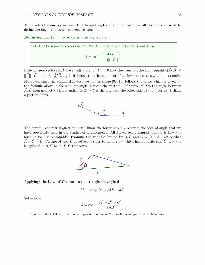
The study of geometry involves lengths and angles of shapes. We have all the tools we need todefine the angle θ between nonzero vectors
Definition 1.1.15. angle between a pair of vectors.
Let ~A, ~B be nonzero vectors in Rn. We define the angle between ~A and ~B by
θ = cos−1[ ~A • ~B
|| ~A|| || ~B||
].
Note nonzero vectors ~A, ~B have || ~A|| 6= 0 and || ~B|| 6= 0 thus the Cauchy-Schwarz inequality | ~A • ~B| ≤|| ~A|| || ~B|| implies
~A • ~B|| ~A|| || ~B||
≤ 1. It follows that the argument of the inverse cosine is within its domain.
Moreover, since the standard inverse cosine has range [0, π] it follows the angle which is given bythe formula above is the smallest angle between the vectors. Of course, if θ is the angle between~A, ~B then geometry clearly indicates 2π − θ is the angle on the other side of the θ vertex. I thinka picture helps:
The careful reader will question how I know the formula really recovers the idea of angle that wehave previously used in our studies of trigonometry. All I have really argued thus far is that theformula for θ is reasonable. Examine the triangle formed by ~A, ~B and ~C = ~B − ~A. Notice that~A + ~C = ~B. Picture ~A and ~B as adjacent sides to an angle θ which has opposite side ~C. Let thelengths of ~A, ~B, ~C be A,B,C respective.
Applying7 the Law of Cosines to the triangle above yields
C2 = A2 +B2 − 2AB cos(θ).
Solve for θ,
θ = cos−1[A2 +B2 − C2
2AB
]7if you had Math 131 with me then you proved the Law of Cosines in one of your first Problem Sets.

24 CHAPTER 1. ANALYTIC GEOMETRY
Is this consistent, does θ = θ ? Choose coordinates8 which place the vectors ~A, ~B, ~C are in thexy-plane and let ~A = 〈A1, A2〉, ~B = 〈B1, B2〉 hence ~C = 〈B1 −A1, B2 −A2〉 we calculate
C2 = (B1 −A1)2 + (B2 −A2)
2 = B21 − 2A1B1 +A2
1 +B22 − 2A2B2 +A2
2
Thus, C2 = A2 +B2 − 2 ~A • ~B and we find:
θ = cos−1[
2 ~A • ~B
2AB
]= cos−1
[ ~A • ~B
|| ~A|| || ~B||
]= θ.
Thus, we find the generalization of angle for Rn agrees with the two-dimensional concept we’veexplored in previous courses. Moreover, we discover a geometrically lucid formula for the dot-product:
~A • ~B = || ~A|| || ~B|| cos(θ)
or if we denote ~A = AA and ~B = BB then
~A • ~B = AB cos(θ).
The connection between this formula and the definition is nontrivial and is essentially equivalentto the Law of Cosines. This means that this is a powerful formula which allows deep calculation ofgeometrically non-obvious angles through the machinery of vectors. Notice:
If ~A, ~B are nonzero orthogonal vectors then the angle between them is π/2.
this observation is an immediate consequence of the the definition of orthogonal vectors and thefact cos(π/2) = 0. We find that orthogonal vectors are in fact perpendicular (which is a knownterm from geometry). In addition,
If ~A, ~B are parallel vectors then ~A • ~B = AB and θ = 0.
likewise,
If ~A, ~B are antiparallel vectors then ~A • ~B = −AB and θ = π.
The dot-product gives us a concrete method to test for whether two vectors point in the samedirection, opposite directions or are purely perpendiular.
8even in the context of Rn we can place ~A, ~B and ~B − ~A in a particular plane, this argument actually extends ton-dimensions provided you accept the Law of Cosines is known in any plane

1.1. VECTORS IN EUCLIDEAN SPACE 25
Example 1.1.16. .
Example 1.1.17. .
We can do more than just measure angles. We can also use the dot-product to project vectors tolines or even planes. In particular:
Definition 1.1.18. projection onto vector.
~A 6= 0 then Proj ~A( ~B) =(~B • A
)A defines the vector projection of ~B onto ~A. We also
define the orthogonal complement of ~B with respect to ~A by Orth ~A( ~B) = ~B − Proj ~A( ~B).
We’ve already seen the projection formula implicitly in the formula ~V = (~V • x) x + (~V • y) ynote that Proj x(~V ) = (~V • x) x since the unit vector of the unit vector x is just x. Likewise,Proj y(~V ) = (~V • y) y. Very well, you might not find this terribly interesting. However, if was toask where a perpendicular bisector of 〈2, 2, 1〉 intersects 〈3, 6, 9〉 then I doubt you could do it withgeometry alone. It’s simple with the projection formula:
Proj〈2,2,1〉(〈1, 2, 3〉
)=[〈1, 2, 3〉 • 〈23 ,
23 ,
13〉]〈23 ,
23 ,
13〉
=[23 + 4
3 + 33
]〈23 ,
23 ,
13〉
= 〈2, 2, 1〉.
26 CHAPTER 1. ANALYTIC GEOMETRY
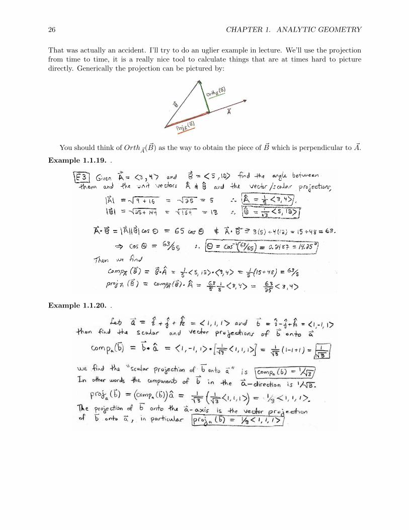
That was actually an accident. I’ll try to do an uglier example in lecture. We’ll use the projectionfrom time to time, it is a really nice tool to calculate things that are at times hard to picturedirectly. Generically the projection can be pictured by:
You should think of Orth ~A( ~B) as the way to obtain the piece of ~B which is perpendicular to ~A.
Example 1.1.19. .
Example 1.1.20. .

1.1. VECTORS IN EUCLIDEAN SPACE 27
Definition 1.1.21. projection and orthogonal complement with respect to a plane.
If ~A, ~B are non-parallel vectors in some plane S then ProjS(~R) =(~R • A
)A +
(~R • B
)B
defines the projection of ~R onto the plane S. The orthogonal projection of ~R off theplane S is given by OrthS(~R) = ~R− ProjS(~R).
The projections onto the coordinate planes are sometimes interesting. Clearly x, y fit in the xy-plane hence
Projxy−plane(〈v1, v2, v3〉) = ( x • 〈v1, v2, v3〉) x+ ( y • 〈v1, v2, v3〉) y = 〈v1, v2, 0〉.
Likewise, Projzx−plane(〈v1, v2, v3〉) = 〈v1, 0, v3〉 and Projyz−plane(〈v1, v2, v3〉) = 〈0, v2, v3〉.
Example 1.1.22. .
Perhaps this material belongs with the larger discussion of planes. I included it here simply toillustrate the utility of the dot-product.
28 CHAPTER 1. ANALYTIC GEOMETRY
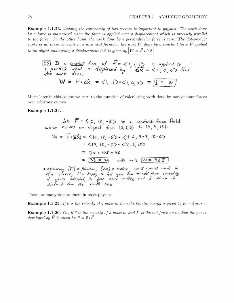
Example 1.1.23. Judging the colinearity of two vectors is important to physics. The work doneby a force is maximized when the force is applied over a displacement which is precisely parallelto the force. On the other hand, the work done by a perpendicular force is zero. The dot-productcaptures all these concepts in a nice neat formula: the work W done by a constant force ~F applied
to an object undergoing a displacement 4~x is given by W = ~F •4~x .
Much later in this course we turn to the question of calculating work done by nonconstant forcesover arbitrary curves.
Example 1.1.24. .
There are many dot-products in basic physics.
Example 1.1.25. If ~v is the velocity of a mass m then the kinetic energy is given by K = 12m~v •~v.
Example 1.1.26. Or, if ~v is the velocity of a mass m and ~F is the net-force on m then the powerdeveloped by ~F is given by P = ~v • ~F .

1.2. THE CROSS PRODUCT 29
1.2 the cross product
We saw that the dot-product gives us a natural way to check if a pair of vectors is orthogonal. Youshould remember: ~A, ~B are orthogonal iff ~A • ~B = 0. We turn to a slightly different goal in thissection: given a pair of nonzero, nonparallel vectors ~A, ~B how can we find another vector ~A × ~Bwhich is perpendicular to both ~A and ~B? Geometrically, in R 3 it’s not too hard to picture it:
My intent in this section is to motivate the standard formula for this product and to prove someof the standard properties of this cross product. These calculations are special to R 3.
Remark 1.2.1.
Forbidden jitzu ahead, In Rn the story is a bit more involved, we can calculate the orthogonalcomplement to span{ ~A, ~B} and this produces an (n − 2)-dimensional space of orthogonalvectors to ~A, ~B. If n = 4 this means there is a whole plane of vectors which we could choose.Only in the case n = 3 is the orthogonal complement simply a one-dimensional space, aline.
Therefore, suppose ~A, ~B are nonzero, nonparallel vectors in R 3. I’ll calculate conditions on ~A× ~Bwhich insure it is perpendicular to both ~A and ~B. Let’s denote ~A × ~B = ~C. We should expect ~Cis some function of the components of ~A and ~B. I’ll use ~A = 〈A1, A2, A3〉 and ~B = 〈B1, B2, B3〉whereas ~C = 〈C1, C2, C3〉
0 = ~C • ~A = C1A1 + C2A2 + C3A3
0 = ~C • ~B = C1B1 + C2B2 + C3B3
Suppose A1 6= 0, then we may solve 0 = ~C • ~A as follows,
C1 = −A2
A1C2 −
A3
A1C3
Suppose B1 6= 0, then we may solve 0 = ~C • ~B as follows,
C1 = −B2
B1C2 −
B3
B1C3
It follows, given the assumptions A1 6= 0 and B1 6= 0,
A2
A1C2 +
A3
A1C3 =
B2
B1C2 +
B3
B1C3

30 CHAPTER 1. ANALYTIC GEOMETRY
Multiply by A1B1 to obtain:
B1A2C2 +B1A3C3 = A1B2C2 +A1B3C3
Thus,(A1B2 −B1A2)C2 + (A1B3 −B1A3)C3 = 0
One solution is simply C2 = A1B3 − B1A3 and C3 = A1B2 − B1A2 and it follows that C1 =A2B3 −B2A3. Of course, generally we could have vectors which are nonzero and yet have A1 = 0or B1 = 0. The point of the calculation is not to provide a general derivation. Instead, my intentis simply to show you how you might be led to make the following definition:
Definition 1.2.2. cross product.
Let ~A, ~B be vectors in R 3. The vector ~A× ~B is called the cross product of ~A with ~B andis defined by
~A× ~B = 〈 A2B3 −A3B2, A3B1 −A1B3, A1B2 −A2B1 〉.
We say ~A cross ~B is ~A× ~B.
It is a simple exercise to verify that
~A • ( ~A× ~B) = 0 and ~B • ( ~A× ~B) = 0.
Both of these identities should be utilized to check your calculation of a given cross product. Let’sthink about the formula for the cross product a bit more. We have
~A× ~B = (A2B3 −A3B2) x1 + (A3B1 −A1B3) x2 + (A1B2 −A2B1) x3
distributing,
~A× ~B = A2B3 x1 −A3B2 x1 +A3B1 x2 −A1B3 x2 +A1B2 x3 −A2B1 x3
The pattern is clear. Each term has indices 1, 2, 3 without repeat and we can generate the signsvia the antisymmetric symbol εijk which is defined be zero if any indices are repeated and
ε123 = ε231 = ε312 = 1 whereas ε321 = ε213 = ε132 = −1.
With this convenient shorthand we find the nice formula for the cross product that follows:
~A× ~B =3∑
i,j,k=1
AiBjεijk xk
Interestingly the Cartesian unit-vectors x1, x2, x3 satisfy the simple relation:
xi × xj =
3∑k=1
εijk xk,

1.2. THE CROSS PRODUCT 31
which is just a fancy way of saying that
x× y = z, y × z = x, z × x = y
There are many popular mneumonics to remember these. The basic properties of the cross producttogether with these formula allow us to quickly calculate some cross products (see Example 1.2.7 )
Proposition 1.2.3. basic properties of the cross product.
Let ~A, ~B, ~C be vectors in R 3 and c ∈ R
1. anticommutative: ~A× ~B = − ~B × ~A,
2. distributive: ~A× ( ~B + ~C) = ~A× ~B + ~A× ~C,
3. distributive: ( ~A+ ~B)× ~C = ~A× ~C + ~B × ~C,
4. scalars factor out: ~A× (c ~B) = (c ~A)× ~B = c ~A× ~B,
Proof: once more, the proof is easy with the right notation. Begin with (1.),
~A× ~B =
3∑i,j,k=1
AiBjεijk xk = −3∑
i,j,k=1
AiBjεjik xk = −3∑
i,j,k=1
BjAiεjik xk = − ~B × ~A.
The key observation was that εijk = −εjik for all i, j, k. If you don’t care for this argument thenyou could also give the brute-force argument below:
~A× ~B = 〈 A2B3 −A3B2, A3B1 −A1B3, A1B2 −A2B1 〉= −〈 A3B2 −A2B3, A1B3 −A3B1, A2B1 −A1B2 〉= −〈 B2A3 −B3A2, B3A1 −B1A3, B1A2 −B2A1 〉= − ~B × ~A. (1.4)
Next, to prove (2.) we once more use the compact notation,
~A× ( ~B + ~C) =3∑
i,j,k=1
Ai(Bj + Cj)εijk xk
=3∑
i,j,k=1
(AiBjεijk xk +AiCjεijk xk)
=
3∑i,j,k=1
AiBjεijk xk +
3∑i,j,k=1
AiCjεijk xk
= ~A× ~B + ~A× ~C.

32 CHAPTER 1. ANALYTIC GEOMETRY
The proof of (3.) follows naturally from (1.) and (2.), note:
( ~A+ ~B)× ~C = −~C × ( ~A+ ~B) = −~C × ~A− ~C × ~B = ~A× ~C + ~B × ~C.
I leave the proof of (4.) to the reader. �
The properties above basically say that the cross product behaves the same as the usual additionand multiplication of numbers with the caveat that the order of factors matters. If we switch theorder then we must include a minus due to the anticommutivity of the cross product.
Example 1.2.4. .
There are a number of popular tricks to remember this rule. Let’s look at a particular example acouple different ways:
Example 1.2.5. .

1.2. THE CROSS PRODUCT 33
Example 1.2.6. .
Therefore,
Technically, this formula is not really a determinant since genuine determinants are formed frommatrices filled with objects of the same type. In the hybrid expression above we actually have onerow of vectors and two rows of scalars. That said, I include it hear since many people use it andI also have found it useful in past calculations. If nothing else at least it helps you learn what adeterminant is. That is a calculation which is worthwhile since determinants have application farbeyond mere cross products.

34 CHAPTER 1. ANALYTIC GEOMETRY
Example 1.2.7. .
The calculation above is probably not the quickest for the example at hand here, but it is fasterfor other computations. For example, suppose ~A = 〈1, 2, 3〉 and ~B = x then
~A× ~B = ( x+ 2 y + 3 z)× x = 2 y × x+ 3 z × x = −2 z + 3 y.
For me, this is quicker than the determinant formula.
Example 1.2.8. once more I contrast the calculational strategies:
1.2. THE CROSS PRODUCT 35
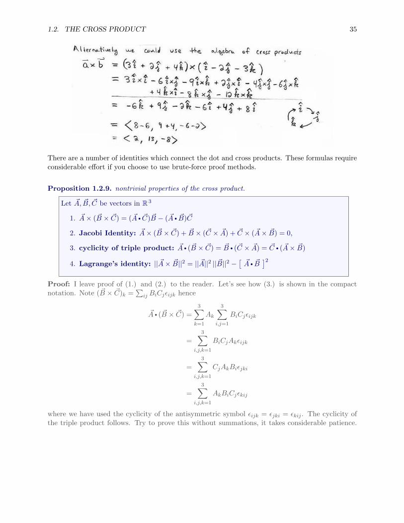
There are a number of identities which connect the dot and cross products. These formulas requireconsiderable effort if you choose to use brute-force proof methods.
Proposition 1.2.9. nontrivial properties of the cross product.
Let ~A, ~B, ~C be vectors in R 3
1. ~A× ( ~B × ~C) = ( ~A • ~C) ~B − ( ~A • ~B)~C
2. Jacobi Identity: ~A× ( ~B × ~C) + ~B × (~C × ~A) + ~C × ( ~A× ~B) = 0,
3. cyclicity of triple product: ~A • ( ~B × ~C) = ~B • (~C × ~A) = ~C • ( ~A× ~B)
4. Lagrange’s identity: || ~A× ~B||2 = || ~A||2 || ~B||2 −[~A • ~B
]2Proof: I leave proof of (1.) and (2.) to the reader. Let’s see how (3.) is shown in the compactnotation. Note ( ~B × ~C)k =
∑ij BiCjεijk hence
~A • ( ~B × ~C) =
3∑k=1
Ak
3∑i,j=1
BiCjεijk
=3∑
i,j,k=1
BiCjAkεijk
=
3∑i,j,k=1
CjAkBiεjki
=3∑
i,j,k=1
AkBiCjεkij
where we have used the cyclicity of the antisymmetric symbol εijk = εjki = εkij . The cyclicity ofthe triple product follows. Try to prove this without summations, it takes considerable patience.

36 CHAPTER 1. ANALYTIC GEOMETRY
Now we turn our attention to Lagrange’s identity. I begin by quoting a useful identity connectingthe antisymmetric symbol and the Kroenecker delta,
3∑k=1
εijkεlmk = δilδjm − δimδjl
Consider that,
|| ~A× ~B||2 =
3∑k=1
( ~A× ~B)2k
=3∑
k=1
( 3∑i,j=1
AiBjεijk
)( 3∑l,m=1
AlBmεlmk
)
=
3∑i,j,k,l,m=1
3∑k=1
AiAlBjBmεijkεlmk
=3∑
i,j,l,m=1
AiAlBjBm(δilδjm − δimδjl)
=3∑
i,j,l,m=1
AiAlδilBjBmδjm −3∑
i,j,l,m=1
AiBmδimBjAlδjl
=
3∑i,j=1
A2iB
2j −
3∑i,j=1
AiBiBjAj
=3∑i=1
A2i
3∑i=1
B2j −
3∑i=1
AiBi
3∑j=1
BjAj
= || ~A||2|| ~B||2 −[~A • ~B
]2.
I leave derivation of the crucial identity to the reader. �.
Use Lagrange’s identity together with ~A • ~B = AB cos(θ),
|| ~A× ~B||2 = A2B2 − [AB cos(θ)]2 = A2B2(1− cos2(θ)) = A2B2 sin2(θ)
It follows there exists some unit-vector n such that
~A× ~B = AB sin(θ)n

1.2. THE CROSS PRODUCT 37
The direction of the unit-vector n is conveniently indicated by the right-hand-rule. I typicallyperform the rule as follows:
1. point fingers of right hand in direction ~A
2. cross the fingers into thr direction of ~B
3. the direction your thumb points is the approximate direction of n
I say approximate because ~A× ~B is strictly perpendicular to both ~A and ~B whereas your thumb’sdirection is a little ambiguous. But, it does pick one side of the plane in which the vectors ~A and~B reside.
Example 1.2.10. .
Example 1.2.11. .

38 CHAPTER 1. ANALYTIC GEOMETRY
Example 1.2.12. .
Example 1.2.13. Another important application of the cross product to physics is the Lorentzforce law. If a charge q has velocity ~v and travels through a magnetic field ~B then the force due tothe electromagnetic interaction between q and the field is ~F = q~v × ~B.
Finally, we should investigate how the dot and cross product give nice formulas for the area of aparallelogram or the volume of a parallel piped. Suppose ~A, ~B give the sides of a parallelogram.
Area = || ~A× ~B ||
The picture below shows why the formula above is true,

1.2. THE CROSS PRODUCT 39
On the other hand, if ~A, ~B, ~C give the corner-edges of a parallelogram then
V olume =∣∣ ~A • ( ~B × ~C)
∣∣These formulas are connected by the following thought: the volume subtended by ~A, ~B and theunit-vector n from ~A× ~B = AB sin(θ)n is equal to the area of the parallelogram with sides ~A, ~B.Algebraically: ∣∣ n • ( ~A× ~B)
∣∣ =∣∣ n • (AB sin(θ)n)
∣∣ = |AB sin(θ)| = || ~A× ~B||.
The picture below shows why the triple product formula is valid.
Example 1.2.14. .
Moreover, given this geometric interpretation we find a new proof (up to a sign) for the cyclicproperty. By the symmetry of the edges it follows that | ~A • ( ~B × ~C) | = | ~B • (~C × ~A) | =| ~C • ( ~A× ~B) |. We should find the same volume no matter how we label width, depth and height.

40 CHAPTER 1. ANALYTIC GEOMETRY
1.3 lines and planes in R 3
There are two main viewpoints to describe lines and planes. The parametric viewpoint introducesparameters which label points on the object of interest. For a line we need one parameter, for aplane we need two parameters. On the other hand, we can view lines and planes just in terms ofthe solution sets of the cartesian coordinates x, y, z. In constrast, we need one equation to describea plane whereas we need two equations to fix a line. In between these two viewpoints is the conceptof a graph. A graph takes one or more of the Cartesian coordinates as parameter(s) and as such itcan easily be thought of as a parametrization. On the other hand, a graph is given by an equationinvolving only cartesian coordinates so it is easy to think of it as a solution set9. Connectingthese viewpoints and gaining a geometric appreciation for both is one of the main themes of thiscourse. Finally, I return to the projection to the plane and we examine the connection between thedot-product based projection and the normal to the plane.
1.3.1 parametrized lines and planes
The parametric equations10 for lines and planes are very natural if you have a proper understandingof vector addition.
Definition 1.3.1. parametrized line.
The line L which points in the ~v-direction and passes through some point ~ro has the naturalparametrization given by
~r(t) = ~ro + t~v
Definition 1.3.2. parametrized plane.
The plane S which contains the point ~ro and the vectors ~A, ~B has a natural parametrizationis given by
~r(u, v) = ~ro + u ~A+ v ~B.
9in later sections we will refer to the solution set formulation as a level set formulation10 I assume the reader has familarity with these terms from calculus II, although, I do provide general definitions
later in this chapter. These are the two most basic examples

1.3. LINES AND PLANES IN R 3 41
If you wish to select a subset of the line or plane above you can appropriately restrict the domainof the parameters. For example, one is often asked to find the parametrization of a line-segmentfrom a point P to a point Q. I recommend the following approach: for 0 ≤ t ≤ 1 let
~r(t) = P (1− t) + tQ.
It’s easy to calculate ~r(0) = P and ~r(1) = Q. This formula can also be written as
~r(t) = P + t(Q− P ) = P + t [−−→PQ].
If we let t go beyond the unit-interval then we trace out the line which contains the line-segment PQ.
Example 1.3.3. Find the parametrization of a line segment which goes from (1, 3) to(5, 2). We use the comment preceding this example and construct:
~r(t) = (1, 3) + t[(5, 2)− (1, 3)] = 〈1 + 4t, 3− t〉
On the other hand, if we wish to parametrize just the parallelogram in the plane with corners ~ro,~ro + ~A, ~ro + ~B and ~ro + ~A + ~B we may limit the values of the parameters u, v to the unit square[0, 1]× [0, 1]; that is, we demand 0 ≤ u ≤ 1 and 0 ≤ v ≤ 1.

42 CHAPTER 1. ANALYTIC GEOMETRY
Example 1.3.4. Find parametrization of plane containing the vectors〈1, 0, 0〉, 〈0, 1, 0〉 and the point (1, 2, 0). We use the natural parametrization:
~r(u, v) = (1, 2, 0) + u〈1, 0, 0〉+ v〈0, 1, 0〉 = (1 + u, 2 + v, 0).
If we allow (u, v) to trace out all of R 2 then we will find the parametrization above covers thexy-plane. Scalar equations which capture the same are x = 1 + u, y = 2 + v, z = 0. If we restrictthe parameters to 0 ≤ u, v ≤ v then the mapping ~r just covers [1, 2]× [2, 3]× {0}.
Example 1.3.5. Suppose ~r(u, v) = (1 + u + v, 2 − u, 3 + v) with (u, v) ∈ R 2 parametrizesa plane. Find the two vectors which lie in the plane and a point on its surface. Thesolution is to work backwards in comparison to the last example. We wish to rip apart the formulaso that we can identify ~ro and ~A, ~B for the given ~r.
~r(u, v) = (1 + u+ v, 2− u, 3 + v) = (1, 2, 3) + u(1,−1, 0) + v(1, 0, 1)
Identify the point (1, 2, 3) is on the plane, in fact it ~r(0, 0) = ~ro. Moreover, the vectors 〈1,−1, 0〉and 〈1, 0, 1〉 lie on the plane. You can verify that 〈1,−1, 0〉 connects ~r(0, 0) = (1, 2, 3) and ~r(1, 0) =(2, 1, 3) whereas 〈1, 1, 0〉 connects ~r(0, 0) = (1, 2, 3) and ~r(0, 1) = (2, 2, 4).
1.3.2 lines and planes as solution sets
Definition 1.3.6. vector equation of plane.
We say that S ⊂ R 3 is a plane with base point ~ro and normal vector ~n iff each ~r ∈ Ssatisfies
(~r − ~ro) •~n = 0. (vector equation of plane)
The geometric motivation for this definition is simple enough: the normal vector is a vector whichis perpendicular to all vectors in the plane. If we take the difference ~r−~ro then this will be a vectorwhich lies on the plane and consequently we must insist they are orthogonal. Here’s a picture ofwhy the definition is reasonable:
Note that the same set of points S can be given many different base points and many differentnormals. This reflects the fact that we can choose the base point anywhere on the plane and the
1.3. LINES AND PLANES IN R 3 43
normal either above or below the plane and can be given many different lengths.
Let ~r = 〈x, y, z〉 be an arbitrary point on the plane S with base point ~ro = 〈xo, yo, zo〉 and normal~n = 〈a, b, c〉 then we can write our plane equation explicitly:
(~r − ~ro) •~n = 0 ⇔ 〈x− xo, y − yo, z − zo〉 • 〈a, b, c〉 = 0
⇔ a(x− xo) + b(y − yo) + c(z − zo) = 0. (scalar equation of plane)
I expect you to know the vector and scalar equations for a plane. We will use both in concept andcalculation.
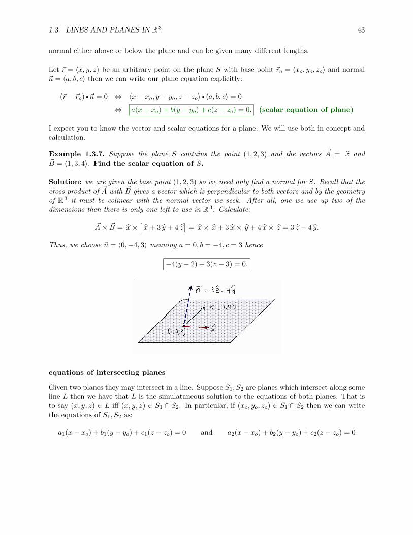
Example 1.3.7. Suppose the plane S contains the point (1, 2, 3) and the vectors ~A = x and~B = 〈1, 3, 4〉. Find the scalar equation of S.
Solution: we are given the base point (1, 2, 3) so we need only find a normal for S. Recall that thecross product of ~A with ~B gives a vector which is perpendicular to both vectors and by the geometryof R 3 it must be colinear with the normal vector we seek. After all, one we use up two of thedimensions then there is only one left to use in R 3. Calculate:
~A× ~B = x×[x+ 3 y + 4 z
]= x× x+ 3 x× y + 4 x× z = 3 z − 4 y.
Thus, we choose ~n = 〈0,−4, 3〉 meaning a = 0, b = −4, c = 3 hence
−4(y − 2) + 3(z − 3) = 0.
equations of intersecting planes
Given two planes they may intersect in a line. Suppose S1, S2 are planes which intersect along someline L then we have that L is the simulataneous solution to the equations of both planes. That isto say (x, y, z) ∈ L iff (x, y, z) ∈ S1 ∩ S2. In particular, if (xo, yo, zo) ∈ S1 ∩ S2 then we can writethe equations of S1, S2 as:
a1(x− xo) + b1(y − yo) + c1(z − zo) = 0 and a2(x− xo) + b2(y − yo) + c2(z − zo) = 0

44 CHAPTER 1. ANALYTIC GEOMETRY
We must solve both at once to find an equation for L. Generally there is no simple formula, howeverif a1, b1, c1, a2, b2, c2 6= 0 then we are free to divide by those constants. First to get the equationsto match divide both by the coefficient of their (z − zo) factor,
a1c1
(x− xo) +b1c1
(y − yo) + z − zo = 0 anda2c2
(x− xo) +b2c2
(y − yo) + z − zo = 0
Thus, solving both equations for z − zo we find,
a1c1
(x− xo) +b1c1
(y − yo) =a2c2
(x− xo) +b2c2
(y − yo)
Multiply by c1c2 and rearrange to find[a1c2 − a2c1
](x− xo) +
[b1c2 − b2c1
](y − yo) = 0
Consequently,x− xo
b1c2 − b2c1=
y − yoa2c1 − a1c2
? .
Following the same algebra we can equally well solve for x− xo,b1a1
(y − yo) +c1a1
(z − zo) =b2a2
(y − yo) +c2a2
(z − zo)
and multiply by a1a2 to find[b1a2 − b2a1
](y − yo) +
[c1a2 − c2a1
](z − zo) = 0
Hence,y − yo
c1a2 − c2a1=
z − zob2a1 − b1a2
? ?.
We combine ? and ?? to obtain the symmetric equations for the line L
x− xob1c2 − b2c1
=y − yo
c2a1 − c1a2=
z − zoc2a1 − c1a2
If we denote ~n1 = 〈a1, b1, c1〉 and ~n2 = 〈a2, b2, c2〉 then recognize that
~w = ~n1 × ~n2 = 〈b1c2 − b2c1, c2a1 − c1a2, c2a1 − c1a2〉
Therefore, with the notation ~w = 〈a, b, c〉, the symmetric equation is simply:
x− xoa
=y − yob
=z − zoc
.
We can use these equations to parametrize the line L. Let t = x−xoa hence x = xo + at is the
parametric equation for x, likewise, y = yo + bt and z = zo + ct. We identify that 〈a, b, c〉 isprecisely the direction-vector for the line L since we can group the scalar parametric equationsabove to obtatin the vector parametric equation below:
~r(t) = 〈xo + at, yo + bt, zo + ct〉 = 〈xo, yo, zo〉+ t〈a, b, c〉.
We find the following interesting geometric result:

1.3. LINES AND PLANES IN R 3 45
The line of intersection for two planes has a direction vector which is colinearwith the cross product of the normals of the intersected planes.
If we take a step back and analyze this by pure geometric visualization this is rediculously obvious.The line of intersection lies in both planes. Therefore, if ~v is the direction vector of L and ~n1 is thenormal of plane S1 and ~n2 is the normal of plane S2 then
1. ~v •~n1 = 0 because ~v lies on S1
2. ~v •~n2 = 0 because ~v lies on S2
3. if ~v is perpendicular to both ~n1 and ~n2 then it must be colinear with ~n1 × ~n2.
This is an example of how geometry is sometimes easier than algebra. In fact, that is often thecase, however, you must get used to both lines of logic in this course. This is the beauty of analyticgeometry.
Let’s examine how we can get from the parametric viewpoint to the symmetric equations. Supposewe are given the vector parametric equations for a line with base point ~ro = (xo, yo, zo) and directionvector ~v = 〈a, b, c〉 with a, b, c 6= 0:
~r(t) = ~ro + t~v = (xo + ta, yo + tb, zo + tc).
Further suppose we denote ~r = 〈x, y, z〉 then the scalar parametric equations for the line are:
x = xo + ta, y = yo + tb, z = zo + tc.
These can be solved for t,x− xoa
=y − yob
=z − zoc
.
and once more we find that the symmetric equations for a line reveal the direction of the line. Well,to be careful, we can multiply this equation by 1/k 6= 0 and we’d still have the same solution setbut a→ ka, b→ kb and c→ kc hence the direction naturally identified would be 〈ka, kb, kc〉. Thisis an ambiguity we always face with lines. The direction vector is not unique, unless we add furthercriteria. For example,
x
2=y
3=z
4

46 CHAPTER 1. ANALYTIC GEOMETRY
suggest the line has direction 〈2, 3, 4〉 whereas
x
−2=
y
−3=
z
−4
suggests the line has direction 〈−2,−3,−4〉.
Finally, recall that I insisted that the intersection of the planes was a line from the outset of thisdiscussion. There is another possibility. It could be that two planes are either parallel and haveno point of intersection, or they could simply be the same plane. In both of those cases the crossproduct of the normals is trivial since the normals of parallel planes are colinear.
1.3.3 lines and planes as graphs
Suppose S is the plane a(x− xo) + b(y− yo) + c(z− zo) = 0 then if c 6= 0 we can solve for z to find
z = zo −a
c(x− xo)−
b
c(y − yo).
If we define f(x, y) = zo − ac (x− xo)− b
c(y − yo) then we can write S as the graph z = f(x, y).
Definition 1.3.8. graphs of f(x, y), g(x, z) or h(y, z).
graph(f) = {(x, y, f(x, y)) | (x, y) ∈ dom(f)}
graph(g) = {(x, g(x, z), z) | (x, z) ∈ dom(g)}
graph(h) = {(h(y, z), y, z) | (y, z) ∈ dom(h)}
clearly S = graph(f) in this context. You could also write S as the graph y = g(x, z) or x = h(y, z)provided b 6= 0 and a 6= 0 respective. I hope you can find the formulas for g or h. These graphsprovide parametrizations as follows, once more consider the case c 6= 0, let
x = u, y = v, z = f(u, v)
Equivalently,
~r(u, v) = 〈u, v, f(u, v)〉.
In this way we find a natural parametrization of a graph. Likewise, if a 6= 0 or b 6= 0 then
~r(u, v) = 〈u, g(u, v), v)〉 or ~r(u, v) = 〈h(u, v), u, v〉
provide natural parametrizations. Parametrizations created in these ways are said to be inducedfrom the graphs g, h respective.
Writing the line as a graph requires us to solve the symmetric equations for two of the cartesiancoordinates in terms of the remaining coordinate. For example, solve for y, z in terms of x:
x− xoa
=y − yob
=z − zoc
⇒ a(y − yo) = b(x− xo) & a(z − zo) = c(x− xo).
1.3. LINES AND PLANES IN R 3 47
hence,
y = yo +b
a(x− xo)︸ ︷︷ ︸
let this be h(x)
& z = zo +c
a(x− xo)︸ ︷︷ ︸
let this be g(x)
Define f(x) = (h(x), g(x)) then graph(f) = {(x, f(x)) | x ∈ R} and it is clear that graph(f) = L.
We say f : R → R 2 is a R 2-valued function of a real variable. Some texts call such functionsmappings whereas they inist that functions are real-valued. I make no such restriction in thesenotes. In any event, there is a natural parametrization which is induced from the graph for L, usex = t hence11
~r(t) = 〈t, f(t)〉 = 〈t, g(t), h(t)〉
parametrizes L. We could also solve for y or z provided b 6= 0 or c 6= 0. I leave those to the reader.
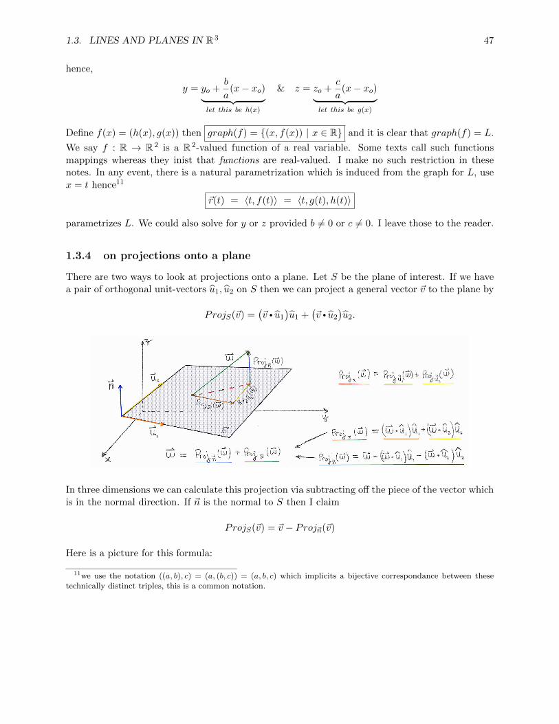
1.3.4 on projections onto a plane
There are two ways to look at projections onto a plane. Let S be the plane of interest. If we havea pair of orthogonal unit-vectors u1, u2 on S then we can project a general vector ~v to the plane by
ProjS(~v) =(~v • u1
)u1 +
(~v • u2
)u2.
In three dimensions we can calculate this projection via subtracting off the piece of the vector whichis in the normal direction. If ~n is the normal to S then I claim
ProjS(~v) = ~v − Proj~n(~v)
Here is a picture for this formula:
11we use the notation ((a, b), c) = (a, (b, c)) = (a, b, c) which implicits a bijective correspondance between thesetechnically distinct triples, this is a common notation.

48 CHAPTER 1. ANALYTIC GEOMETRY
Let’s see why in n = 3 these formulas are equivalent. Construct the normal corresponding to theunit vectors in the usual manner: ~n = u1 × u2. Orthogonality of the unit vectors implies θ = π
2hence ||u1 × u2|| = 1 and it follows ~n = n. Let us define
ProjS(~v) = ~v − (~v • n)n ?
Observe this formula produces a vector on the plane,
ProjS(~v) • n = ~v • n− (~v • n)n • n = ~v • n− ~v • n = 0.
Notice that n • u1 = 0 and n • u2 = 0. Take the dot-product of ? with u1 and u2 to obtain,
ProjS(~v) • u1 = ~v • u1 and ProjS(~v) • u2 = ~v • u2
It follows that ProjS(~v) =(~v • u1
)u1 +
(~v • u2
)u2. The formulas agree. They both produce the
same projection onto the plane. If we attach ~v to the plane at some point P ∈ S then ProjS(~v)attached to P will point to the point on the plane S which is closest to the end of the vector ~v.
Perhaps the example that follows will help you understand the discussion above.
Example 1.3.9. Let S be the plane through (0, 0, 1) with normal ~n = 〈1, 0, 1〉. Notice that ~u1 =〈1, 0,−1〉 and ~u2 = 〈0, 1, 0〉 are orthogonal as ~u1 • ~u2 = 0 and they are both on S as ~n • ~u1 = 0 and~n • ~u2 = 0. Normalize the vectors,
u1 =1√2〈1, 0,−1〉, u2 = 〈0, 1, 0〉 n =
1√2〈1, 0, 1〉
Let ~v = 〈a, b, c〉. Calculate,
ProjS(~v) =(~v • u1
)u1 +
(~v • u2
)u2
=1
2
(a− c
)〈1, 0,−1〉+ b〈0, 1, 0〉
= 〈 1
2(a− c), b, 1
2(c− a) 〉.

1.3. LINES AND PLANES IN R 3 49
On the other hand, the normal formula says,
ProjS(~v) = ~v − (~v • n)n
= 〈a, b, c〉 − 1
2(a+ c)〈1, 0, 1〉
= 〈a− 1
2(a+ c), b, c− 1
2(a+ c)〉
= 〈 1
2(a− c), b, 1
2(c− a) 〉.
We typically use the normal formulation of the projection since it’s easier to find a normal than it isto find a pair of orthonormal vectors on the plane. That said, the orthonormal projection formulanaturally generalizes to higher dimensional studies. We discuss applications of such formulas inlinear algebra. It is the math behind least squares data fitting and Fourier analysis.
Example 1.3.10. .

50 CHAPTER 1. ANALYTIC GEOMETRY
1.3.5 additional examples
Example 1.3.11. .
Example 1.3.12. .
Example 1.3.13. .
Example 1.3.14. .

1.3. LINES AND PLANES IN R 3 51
Example 1.3.15. .
Example 1.3.16. .

52 CHAPTER 1. ANALYTIC GEOMETRY
Example 1.3.17. .
Example 1.3.18. .

1.3. LINES AND PLANES IN R 3 53
Example 1.3.19. .
Example 1.3.20. .

54 CHAPTER 1. ANALYTIC GEOMETRY
1.4 curves
A curve is a one-dimensional subset of some space. There are at least three common, but distinct,ways to frame the mathematics of a curve. These viewpoints were already explored in the previoussection but I list them once more: we can describe a curve:
1. as a path, that is as a parametrized curve.
2. as a level curve, also known as a solution set.
3. as a graph.
I expect you master all three viewpoints in the two-dimensional context. However, for three or moredimensions we primarily use the parametric viewpoint in this course. Exceptions to this rule arefairly rare: the occasional homework problem where you are asked to find the curve of intersectionfor two surfaces, or the symmetric equations for a line. In contrast, the parametric decription ofa curve in three dimensions is far more natural. Do you want to describe a curve as where twosurfaces intersect or would you rather describe a curve as a set of points formed by pasting a copyof the real line through your space? I much prefer the parametric view.
Definition 1.4.1. vector-valued functions, curves and paths.
A vector valued function of a real variable is an assignment of a vector for each real numberin some domain. It’s a mapping t 7→ ~f(t) =
⟨f1(t), f2(t), . . . , fn(t)
⟩for each t ∈ J ⊂ R.
We say fj : J ⊆ R → R is the j-th component function of ~f . Let C = ~f(J) then C is said
to be a curve which is parametrized by ~f . We can also say that t 7→ ~f(t) is a path inRn. Equivalently, but not so usefully, we can write the scalar parametric equations for Cabove as
x1 = f1(t), x2 = f2(t), . . . , xn = fn(t)
for all t ∈ J .
When we define a parametrization of a curve it is important to give the formula for the path andthe domain of the parameter. Note that when I say the word curve I mean for us to think aboutsome set of points, whereas when I say the word path I mean to refer to the particular mappingwhose image is a curve. We may cover a particular curve with infinitely many different paths.
1.4.1 curves in two-dimensional space
We have several viewpoints to consider. Graphs, parametrized curves and level sets.
graphs in the plane
Let’s begin by reminding ourselves of the definition of a graph:
1.4. CURVES 55
Definition 1.4.2. Graph of a function.
Let f : dom(f)→ R be a function then
graph(f) = {(x, f(x)) | x ∈ dom(f)}.
We know this is quite restrictive. We must satisfy the vertical line test if we say our curve is thegraph of a function.
Example 1.4.3. To form a circle centered at the origin of radius R we need to glue together twographs. In particular we solve the equation x2 + y2 = R2 for y =
√R2 − x2 or y = −
√R2 − x2.
Let f(x) =√R2 − x2 and g(x) = −
√R2 − x2 then we find graph(f) ∪ graph(g) gives us the whole
circle.
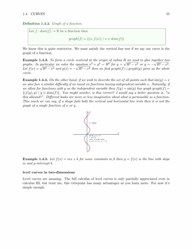
Example 1.4.4. On the other hand, if we wish to describe the set of all points such that sin(y) = xwe also face a similar difficulty if we insist on functions having independent variable x. Naturally, ifwe allow for functions with y as the independent variable then f(y) = sin(y) has graph graph(f) ={(f(y), y) | y ∈ dom(f)}. You might wonder, is this correct? I would say a better question is, ”isthis allowed?”. Different books are more or less imaginative about what is permissible as a function.This much we can say, if a shape fails both the vertical and horizontal line tests then it is not thegraph of a single function of x or y.
Example 1.4.5. Let f(x) = mx + b for some constants m, b then y = f(x) is the line with slopem and y-intercept b.
level curves in two-dimensions
Level curves are amazing. The full calculus of level curves is only partially appreciated even incalculus III, but trust me, this viewpoint has many advantages as you learn more. For now it’ssimple enough:

56 CHAPTER 1. ANALYTIC GEOMETRY
Definition 1.4.6. Level Curve.
A level curve is given by a function of two variables F : dom(F ) ⊆ R2 → R and a constantk. In particular, the set of all (x, y) ∈ R2 such that F (x, y) = k is called the level-set of F ,but more commonly we just say F (x, y) = k is a level curve.
In an algebra class you might have called this the ”graph of an equation”, but that terminologyis dead to us now. For us, it is a level curve. Moreover, for a particular set of points C ⊆ R2
we can find more than one function F which produces C as a level set. Unlike functions, for aparticular curve there is not just one function which returns that curve. This means that it mightbe important to give both the level-function F and the level k to specify a level curve F (x, y) = k.
Example 1.4.7. A circle of radius R centered at the origin is a level curve F (x, y) = R2 whereF (x, y) = x2 + y2. We call F the level function (of two variables).
Example 1.4.8. To describe sin(y) = x as a level curve we simply write sin(y)−x = 0 and identifythe level function is F (x, y) = sin(y)− x and in this case k = 0. Notice, we could just as well sayit is the level curve G(x, y) = 1 where G(x, y) = x− sin(y) + 1.
Note once more this type of ambiguity is one distinction of the level curve langauge, in constrast,the graph graph(f) of a function y = f(x) and the function f are interchangeable. Some mathe-maticians insist the rule x 7→ f(x) defines a function whereas others insist that a function is a setof pairs (x, f(x)). I prefer the mapping rule because it’s how I think about functions in generalwhereas the idea of a graph is much less useful in general.
Example 1.4.9. A line with slope m and y-intercept b can be described by F (x, y) = mx+b−y = 0.Alternatively, a line with x-intercept xo and y-intercept yo can be described as the level curveG(x, y) = x
xo+ y
yo= 1.
Example 1.4.10. Level curves need not be simple things. They can be lots of simple things gluedtogether in one grand equation:
F (x, y) = (x− y)(x2 + y2 − 1)(xy − 1)(y − tan(x)) = 0.
Solutions to the equation above include the line y = x, the unit circle x2+y2 = 1, the tilted-hyperbolaknown more commonly as the reciprocal function y = 1
x and finally the graph of the tangent. Someof these intersect, others are disconnected from each other.
It is sometimes helpful to use software to plot equations. However, we must be careful since theyare not as reliable as you might suppose. The example above is not too complicated but look whathappens with Graph:

1.4. CURVES 57
Theorem 1.4.11. any graph of a function can be wriiten as a level curve.
If y = f(x) is the graph of a function then we can write F (x, y) = f(x)− y = 0 hence thegraph y = f(x) is also a level curve.
Not much of a theorem. But, it’s true. The converse is not true without a lot of qualification. I’llstate that theorem (it’s called the implicit function theorem) in a future chapter after we’ve studiedpartial differentiation.
parametrized curves in two-dimensions
Example 1.4.12. Suppose a, b〉0 and h, k ∈ R. The parametrization
~r(t) = 〈h+ a cos(t), k + b sin(t)〉
for t ∈ [0, 2π] coveres and the ellipse
(x− h)2
a2+
(y − k)2
b2= 1.
Example 1.4.13. Suppose a, b〉0 and h, k ∈ R. The parametrization
~r1(t) = 〈h+ a cosh(t), k + b sinh(t)〉
for t ∈ R coveres one branch of the hyperbola
(x− h)2
a2− (y − k)2
b2= 1.
Note x = h+ a cosh(t) implies x−ha = cosh(t) ≥ 1 therefore it follows x ≥ h+ a. We’ve covered the
right branch. If we wish to cover the left branch of this hyperbola then use:
~r2(t) = 〈h− a cosh(t), k + b sinh(t)〉.

58 CHAPTER 1. ANALYTIC GEOMETRY
Example 1.4.14. A spiral can be thought of as a sort of circle with a variable radius. With thatin mind I write: for t ≥ 0,
~r(t) = 〈t cos(t), t sin(t)〉
to give a spiral whose ”radius” is proportional to the angle t subtended from t = 0.
Finding the parametric equations for a curve does require a certain amount of creativity. However,it’s almost always some slight twist on the examples I give in this section. The remaining examplesI also give in calculus II, I add some detail to emphasize how the parametrization matches thealready known identities of certain curves and I add pictures which emphasize the idea that theparametrization pastes a line into R 2.
Example 1.4.15. Let x = R cos(t) and y = R sin(t) for t ∈ [0, 2π]. This is a parametrization ofthe circle of radius R centered at the origin. We can check this by substituting the equations backinto our standard Cartesian equation for the circle:
x2 + y2 = (R cos(t))2 + (R sin(t))2 = R2(cos2(t) + sin2(t))
Recall that cos2(t) + sin2(t) = 1 therefore, x(t)2 + y(t)2 = R2 for each t ∈ [0, 2π]. This shows thatthe parametric equations do return the set of points which we call a circle of radius R. Moreover,we can identify the parameter in this case as the standard angle from standard polar coordinates.

1.4. CURVES 59
Example 1.4.16. Let x = R cos(et) and y = R sin(et) for t ∈ R. We again cover the circle at tvaries since it is still true that (R cos(et))2 + (R sin(et))2 = R2(cos2(et) + sin(et)) = R2. However,since range(et) = [1,∞) it is clear that we will actually wrap around the circle infinitly many times.The parametrizations from this example and the last do cover the same set, but they are radicallydifferent parametrizations: the last example winds around the circle just once whereas this examplewinds around the circle ∞-ly many times.
Example 1.4.17. Let x = R cos(−t) and y = R sin(−t) for t ∈ [0, 2π]. This is a parametrizationof the circle of radius R centered at the origin. We can check this by substituting the equations backinto our standard Cartesian equation for the circle:
x2 + y2 = (R cos(−t))2 + (R sin(−t))2 = R2(cos2(−t) + sin2(−t))
Recall that cos2(−t)+sin2(−t) = 1 therefore, x(t)2+y(t)2 = R2 for each t ∈ [0, 2π]. This shows thatthe parametric equations do return the set of points which we call a circle of radius R. Moreover,we can identify the parameter an angle measured CW12 from the positive x-axis. In contrast, thestandard polar coordinate angle is measured CCW from the postive x-axis. Note that in this examplewe cover the circle just once, but the direction of the curve is opposite that of Example 1.4.15.
12CW is an abbreviation for ClockWise,whereas CCW is an abbreviation for CounterClockWise.

60 CHAPTER 1. ANALYTIC GEOMETRY
The idea of directionality is not at all evident from Cartesian equations for a curve. Given a graphy = f(x) or a level-curve F (x, y) = k there is no intrinsic concept of direction ascribed to the curve.For example, if I ask you whether x2 + y2 = R2 goes CW or CCW then you ought not have ananswer. I suppose you could ad-hoc pick a direction, but it wouldn’t be natural. This means thatif we care about giving a direction to a curve we need the concept of the parametrized curve. Wecan use the ordering of the real line to induce an ordering on the curve.
Definition 1.4.18. oriented curve.
Suppose f, g : J ⊆ R → R are 1 − 1 functions. We say the set {(f(t), g(t)) | t ∈ J} is anoriented curve and say t→ (f(t), g(t)) is a consistently oriented path which covers C. IfJ = [a, b] and (f(a), g(a)) = p and (f(b), g(b)) = q then we can say that C is a curve fromto p to q.
I often illustrate the orientation of a curve by drawing little arrows along the curve to indicate thedirection. Furthermore, in my previous definition of parametrization I did not insist the parametricfunctions were 1 − 1, this means that those parametrizations could reverse direction and go backand forth along a given curve. What is meant by the terms ”path”, ”curve” and ”parametricequations” may differ from text to text so you have to keep a bit of an open mind and try to letcontext be your guide when ambguity occurs. I will try to be uniform in my langauge within thiscourse.
Example 1.4.19. The line y = 3x + 2 can be parametrized by x = t and y = 3t + 2 for t ∈ R.This induces an orientation which goes from left to right for the line. On the other hand, if weuse x = −λ and y = −3λ+ 2 then as λ increases we travel from right to left on the curve. So theλ-equations give the line the opposite orientation.

1.4. CURVES 61
To reverse orientation for x = f(t), y = g(t) for t ∈ J = [a, b] one may simply replace t by−t in the parametric equations, this gives new equations which will cover the same curve viax = f(−t), y = g(−t) for t ∈ [−a,−b].
Example 1.4.20. The line-segment from (0,−1) to (1, 2) can be parametrized by x = t and y =3t− 1 for 0 ≤ t ≤ 1. On the other hand, the line-segment from (1, 2) to (0,−1) is parametrized byx = −t, y = −3t− 1 for −1 ≤ t ≤ 0.
The other method to graph parametric curves is simply to start plugging in values for the parameterand assemble a table of values to plot. I have illustrated that in part by plotting the green dots inthe domain of the parameter together with their images on the curve. Those dots are the results ofplugging in the parameter to find corresponding values for x, y. I don’t find that is a very reliableapproach in the same way I find plugging in values to f(x) provides a very good plot of y = f(x).That sort of brute-force approach is more appropriate for a CAS system. There are many excellenttools for plotting parametric curves, hopefully I will have some posted on the course website. Inaddition, the possibility of animation gives us an even more exciting method for visualization of the
62 CHAPTER 1. ANALYTIC GEOMETRY
time-evolution of a parametric curve. In the next chapter we connect the parametric viewpoint withphysics and such an animation actually represents the physical motion of some object. My focusin the remainder of this chapter is almost purely algebraic, I could draw pictures to explain, but Iwanted the notes to show you that the pictures are not necessary when you understand the algebraicprocess. That said, the best approach is to do some combination of algebraic manipulation/figuringand graphical reasoning.
converting to and from the parametric viewpoint in 2D
Let’s change gears a bit, we’ve seen that parametric equations for curves give us a new methodto describe particular geometric concepts such as orientability or multiple covering. Without theintroduction of the parametric concept these geometric ideas are not so easy to describe. That said,I now turn to the question of how to connect parametric descriptions with Cartesian descriptionsof a curve. We’d like to understand how to go both ways if possible:
1. how can we find the Cartesian form for a given parametric curve?
2. how can we find a parametrization of a given Cartesian curve?
In case (2.) we mean to include the ideas of level curves and graphs. It turns out that bothquestions can be quite challenging for certain examples. However, in other cases, not so much: forexample any graph y = f(x) is easily recast as the set of parametric equations x = t and y = f(t)for t ∈ dom(f). For the standard graph of a function we use x as the parameter.
1.4.2 how can we find the Cartesian form for a given parametric curve?
Example 1.4.21. What curve has parametric equations x = t for y = t2 for t ∈ R? To findCartesian equation we eliminate the parameter (when possible)
t2 = x2 = y ⇒ y = x2
Thus the Cartesian form of the given parametrized curve is simply y = x2.
Example 1.4.22. Example 15.2.2: Find parametric equations to describe the graph y =√x+ 3
for 0 ≤ x < ∞. We can use x = t2 and y =√t2 + 3 for t ∈ R. Or, we could use x = λ and
y =√λ+ 3 for λ ∈ [0,∞).
Example 1.4.23. What curve has parametric equations x = t for y = t2 for t ∈ [0, 1]? To findCartesian equation we eliminate the parameter (when possible)
t2 = x2 = y ⇒ y = x2
Thus the Cartesian form of the given parametrized curve is simply y = x2, however, given that0 ≤ t ≤ 1 and x = t it follows we do not have the whole parabola, instead just y = x2 for 0 ≤ x ≤ 1.

1.4. CURVES 63
Example 1.4.24. Identify what curve has parametric equations x = tan−1(t) and y = tan−1(t) fort ∈ R. Recall that range(tan−1(t)) = (−π/2, π/2). It follows that −π/2 < x < π/2. Naturally wejust equate inverse tangent to obtain tan−1(t) = y = x. The curve is the open line-segment withequation y = x for −π/2 < x < π/2. This is an interesting parameterization, notice that as t→∞we approach the point (π/2, π/2), but we never quite get there.
Example 1.4.25. Consider x = ln(t) and y = et − 1 for t ≥ 1. We can solve both for t to obtain
t = ex = ln(y + 1) ⇒ y = −1 + exp(exp(x)).
The domain for the expression above is revealed by analyzing x = ln(t) for t ≥ 1, the image of[1,∞) under natural log is precisely [0,∞); ln[1,∞) = [0,∞).
Example 1.4.26. Suppose x = cosh(t)− 1 and y = 2 sinh(t) + 3 for t ∈ R. To eliminate t it helpsto take an indirect approach. We recall the most important identity for the hyperbolic sine andcosine: cosh2(t) − sinh2(t) = 1. Solve for hyperbolic cosine; cosh(t) = x + 1. Solve for hyperbolicsine; sinh(t) = y−3
2 . Now put these together via the identity:
cosh2(t)− sinh2(t) = 1 ⇒ (x+ 1)2 − (y − 3)2
4= 1.
Note that cosh(t) ≥ 1 hence x + 1 ≥ 1 thus x ≥ 0 for the curve described above. On the otherhand y is free to range over all of R since hyperbolic sine has range R. You should13 recognize theequation as a hyperbola centered at (−1, 3).
how can we find a parametrization of a given Cartesian curve?
I like this topic more, the preceding bunch of examples, while needed, are boring. The art ofparameterizing level curves is much more fun.
Example 1.4.27. Find parametric equations for the circle centered at (h, k) with radiusR.
To begin recall the equation for such a circle is (x − h)2 + (y − k)2 = R2. Our inspiration is theidentity cos( t) + sin2(t) = 1. Let x− h = R cos(t) and y − k = R sin(t) thus
x = h+R cos(t) and y = k +R sin(t).
I invite the reader to verify these do indeed parametrize the circle by explicitly plugging in theequations into the circle equation. Notice, if we want the whole circle then we simply choose anyinterval for t of length 2π or longer. On the other hand, if you want to select just a part of thecircle you need to think about where sine and cosine are positive and negative. For example, if Iwant to parametrize just the part of the circle for which x > h then I would choose t ∈ (−π
2 ,π2 ).
13many students need to review these at this point, we use circles, ellipses and hyperbolas as examples in thiscourse. I’ll give examples of each in this chapter.

64 CHAPTER 1. ANALYTIC GEOMETRY
The reason I choose that intuitively is that the parametrization given for the circle above is basicallybuilt from polar coordinates14 centered at (h, k). That said, to be sure about my choice of parameterdomain I like to actually plug in some of my proposed domain and make sure it matches thedesired criteria. I think about the graphs of sine and cosine to double check my logic. I know thatcos(−π
2 ,π2 ) = (0, 1] whereas sin(−π
2 ,π2 ) = (−1, 1), I see it in my mind. Then I think about the
parametric equations in view of those facts,
x = h+R cos(t) and y = k +R sin(t).
I see that x will range over (h, h+R] and y will range over (k −R, k +R). This is exactly what Ishould expect geometrically for half of the circle. Visualize that x = h is a vertical line which cutsour circle in half. These are the thoughts I think to make certain my creative leaps are correct. Iwould encourage you to think about these matters. Don’t try to just memorize everything, it willnot work for you, there are simply too many cases. It’s actually way easier to just understand theseas a consequence of trigonometry, algebra and analytic geometry.
14we will discuss further in a later section, but this should have been covered in at least your precalculus course.

1.4. CURVES 65
Example 1.4.28. Find parametric equations for the level curve x2 + 2x+ 14y
2 = 0 whichgive the ellipse a CW orientation.
To begin we complete the square to understand the equation:
x2 + 2x+1
4y2 = 0 ⇒ (x+ 1)2 +
1
4y2 = 1.
We identify this is an ellipse centered at (−1, 0). Again, I use the pythagorean trig. identity as myguide: I want (x+ 1)2 = cos2(t) and 1
4y2 = sin2(t) because that will force the parametric equations
to solve the ellipse equation. However, I would like for the equations to describe CW direction so Ireplace the t with −t and propose:
x = −1 + cos(−t) and y = 2 sin(−t)
If we choose t ∈ [0, 2π) then the whole ellipse will be covered. I could simplify cos(−t) = cos(t) andsin(−t) = − sin(t) but I have left the minus to emphasize the idea about reversing the orientation.In the preceding example we gave the circle a CCW orientation.
Example 1.4.29. Find parametric equations for the part of the level curve x2 − y2 = 1which is found in the first quadrant.
We recognize this is a hyperbola which opens horizontally since x = 0 gives us −y2 = 1 whichhas no real solutions. Hyperbolic trig. functions are built for a problem just such as this: recallcosh2(t) − sinh2(t) = 1 thus we choose x = cosh(t) and y = sinh(t). Furthermore, the hyperbolicsine function sinh(t) = 1
2
(et − e−t
)is everywhere increasing since it has derivative cosh(t) which
is everywhere positive. Moreover, since sinh(0) = 0 we see that sinh(t) ≥ 0 for t ≥ 0. Choosenon-negative t for the domain of the parametrization:
x = cosh(t), y = sinh(t), t ∈ [0,∞).
Example 1.4.30. Find parametric equations for the part of the level curve x2 − y2 = 1which is found in the third quadrant.
Based on our thinking from the last example we just need to modify the solution a bit:
x = − cosh(t), y = sinh(t), t ∈ (−∞, 0].
Note that if t ∈ (−∞, 0] then − cosh(t) ≤ −1 and sinh(t) ≤ 0, this puts us in the third quadrant. Itis also clear that these parametric equations to solve the hyperbola equation since
(− cosh(t))2 − (sinh(t))2 = cosh2(t)− sinh2(t) = 1.
The examples thus far are rather specialized, and in general there is no method to find parametricequations. This is why I said it is an art.

66 CHAPTER 1. ANALYTIC GEOMETRY
Example 1.4.31. Find parametric equations for the level curve x2y2 = x− 2.
This example is actually pretty easy because we can solve for y2 = x−2x2
hence y = ±√
x−2x2
. We can
choose x as parameter so the parametric equations are just
x = t and y =
√t− 2
t2
for t ≥ 2. Or, we could give parametric equations
x = t and y = −√t− 2
t2
for t ≥ 2. These parametrizations simply cover different parts of the same level curve.
Remark 1.4.32. but... what is t ?
If you are at all like me when I first learned about parametric curves you’re probablywondering what is t ? You probably, like me, suppose incorrectly that t should be justlike x or y. There is a crucial difference between x and y and t. The notations x and yare actually shorthands for the Cartesian coordinate maps x : R2 → R and y : R2 → Rwhere x(a, b) = a and y(a, b) = b. When I use the notaion x = 3 then you know whatI mean, you know that I’m focusing on the vertical line with first coordinate 3. On theother hand, if I say t = 3 and ask where is it? Then you should say, you question doesn’tmake sense. The concept of t is tied to the curve for which it is the parameter. There areinfinitely many geometric meanings for t. In other words, if you try to find t in the xy-plane without regard to a curve then you’ll never find an answer. It’s a meaningless question.
On the other hand if we are given a curve and ask what the meaning of t is for that curvethen we ask a meaningful question. There are two popular meanings.
1. the parameter s measures the arclength from some base point on the given curve.
2. the parameter t gives the time along the curve.
In case (1.) for an oriented curve this actually is uniquely specified if we have a startingpoint. Such a parameterization is called the arclength parametrization or unit-speedparametrization of a curve. These play a fundamental role in the study of the differentialgeometry of curves. In case (2.) we have in mind that the curve represents the physicaltrajectory of some object, as t increases, time goes on and the object moves. I tend touse (2.) as my conceptual backdrop. But, keep in mind that these are just applications ofparametric curves. In general, the parameter need not be time or arclength. It might justbe what is suggested by algebraic convenience.

1.4. CURVES 67
1.4.3 curves in three dimensional space
Other interesting curves can be obtained by feeding a simple curve like a circle into the parame-terization of a plane.
Example 1.4.33. Suppose ~R(u, v) = ~ro + u ~A+ v ~B is the parametrization of a plane S then if wecompose ~R with the path t 7→ ~γ(t) = 〈R cos(t), R sin(t)〉 we obtain an ellipse on the plane:
~r(t) = (~R ◦~γ)(t) = ~ro +R cos(t) ~A+R sin(t) ~B
Of course, we could also put a spiral on a plane through much the same device:
The idea of the last example can be used to create many interesting examples. These should sufficefor our purposes here. I really just want you to think about what a parametrization does. Moreover,I hope you can find it in your heart to regard the parametric viewpoint as primary. Notice that anycurves in three dimensions would require two independent equations in x, y, z. We saw how muchof a hassel this was for something as simple as a line. I’d rather not attempt a general treatmentof the purely cartesian description of the curves in this section15 I instead offer a pair of examplesto give you a flavor:
Example 1.4.34. Suppose x2 + y2 + z2 = 4 and x =√
2 then the solution set of this pair ofequations defines a curve in R 3. Substutiting x =
√3 into x2 + y2 + z2 = 4 gives y2 + z2 = 1. The
solution set is just a unit-circle in the yz-coordinates placed at x =√
3. We can parametrize it via:
~r(t) = 〈√
3, cos t, sin t〉.
Example 1.4.35. Suppose z = x2 − y2 and z = 2x. The solution set is once more a curve in R 3.We can substitute z = 2x into z = x2 − y2 to obtain x2 − y2 = 2x hence x2 − 2x − y2 = 0 andcompleting the square reveals (x − 1)2 − y2 = 1. This is the equation of a hyperbola. A naturalparametrization is given by x = 1+cosh t and y = sinh t then since z = 2x we have z = 2+2 cosh t.In total,
~r(t) = 〈1 + cosh t, sinh t, 2 + 2 cosh t〉
We’ll explain the geometry of these calculations in the next section. Basically the idea is justthat when two surfaces intersect in R 3 we may obtain a curve.
15which is not to say it hasn’t been done, in fact, viewing curves as solutions to equations is also a powerfultechnique, but we focus our efforts in the parametric setting.

68 CHAPTER 1. ANALYTIC GEOMETRY
Example 1.4.36. A helix of radius R which wraps around the z-axis and has a slope of m is givenby:
~r(t) = 〈R cos(t), R sin(t),mt〉
for t ∈ [0,∞).
Example 1.4.37. The curve parametrized by ~r(t) = 〈t, t2, t3 for t ≥ 0 has scalar parametricequations x = t, y = t2, z = t3 and a graph
Example 1.4.38. The curve parametrized by ~r(t) = 〈t, t2 cos(3t), t3 sin(3t)〉 for t ≥ 0 has scalarparametric equations x = t, y = t2 cos(t), z = t3 sin(t) and a graph
Example 1.4.39. The curve parametrized by ~r(t) = 〈t cos(3t), t2 sin(3t), t3〉 for t ≥ 0 has scalarparametric equations x = t cos(3t), y = t2 sin(3t), z = t3 and a graph

1.4. CURVES 69
We will explore the geometry of curves in the next chapter. We’ll find relatively simple calculationswhich allow us to test how a curve bends within it’s plane of motion and bend off it’s plane ofmotion. In other words, we’ll find a way to test if a curve lies in a plane and also how it curvesaway from it’s tangential direction. These quantities are called torsion and curvature. It turnsout that these two quantities often classify a curve upto congruence in the sense of high-schoolgeometry. In other words, there is just one circle of radius 1 and we can rotate it and translate itthroughout R 3. In this sense all circles in R 3 are the same. We’ve already seen in this section thatparametrization alone does not capture this concept. Why? Well there are many parametrizationsof a circle. Are those different circles? I would say not. I say there is a circle and there are manypictures of the circle, some CW, some CCW, but so long as those pictures cover the same curvethen they are merely differing perspectives on the same object. That said, these differing picturesare different. They are unique in their assignments of points to parameter values. The problemof the differential geometry of curves is to extract from this infinity of parametrizations someuniversal data. One seeks a few constants which invariantly characterize the curve independent ofthe perspective a particular geometer has used to capture it. More generally this is the problem ofgeometry. How can we classify spaces? What constants can we label a space with unambiguously?

70 CHAPTER 1. ANALYTIC GEOMETRY
1.5 surfaces
A surface in R 3 is a subset which usually looks two dimensional. There are three main viewpoints;graphs, parametrizations or patches, and level-surfaces. As usual, the parametric view naturallygeneralizes to surfaces in Rn for n > 3 with relatively little qualification. That said, we almostwithout exception focus on surfaces in R 3 in this course so I focus our efforts in that direction.This section is introductory in nature, basically this is just show and tell with a little algebra. Yourgoal should be to learn the names of these surfaces and more importantly to gain a conceptualfoothold on the different ways to look at two-dimensional subsets of R 3. Many of the diagrams inthis section were created with Maple, others perhaps Mathematica. Ask if interested.
1.5.1 surfaces as graphs
Given a function of two variables it is natural to graph such a function in three-dimensions. Inparticular, we define:
Definition 1.5.1. graph of a function of two variables.
Suppose f : dom(f) ⊆ R 2 → R is a function then the set of all (x, y, z) such that z = f(x, y)for some (x, y) ∈ dom(f) is called the graph of f . Moreover, we denote graph(f) ={(x, y, f(x, y)) | (x, y) ∈ dom(f)}.
Example 1.5.2. Let f(x, y) = xe−x2−y2. The graph looks something like:
Example 1.5.3. Let f(x, y) = −cosh(xy). The graph looks something like:

1.5. SURFACES 71
What is f? Well, many interpretations exist. For example, f could represent the temperature at(x, y). Or, f could represent the mass per unit area close to (x, y), this would make f a massdensity function. More generally, if you have a variable which depends by some single-valued ruleto another pair of variables then you can find a function in that application. Sometimes collegealgebra students will ask, but what is a function really? With a little imagination the answer ismost anything. It could be that f is the cost for making x widgets and y gadgets. Or, perhapsf(x, y) is the grade of a class as a function of x males and y females. Enough. Let’s get back tothe math, I’ll generally avoid cluttering these notes with these silly comments, however, you arefree to ask in office hours. Not all such discussion is without merit. Application is important, butis not at all necessary for good mathematics.
We can add, multiple and divide functions of two variables in the same way we did for functionsof one variable. Natural domains are also implicit within formulas and points are excluded formuch the same reason as in single-variable calculus; we cannot divide by zero, take an even rootof a negative number or take a logarithm of a non-positive quantity if we wish to maintain a realoutput16. A typical example is given below:
Example 1.5.4. .
16complex variables do give meaning to even roots and logarithms of negative numbers however, division by zeroand logarithm of zero continue to lack an arithmetical interpretation.

72 CHAPTER 1. ANALYTIC GEOMETRY
1.5.2 parametrized surfaces
Definition 1.5.5. vector-valued functions of two real variables, parametrized surfaces.
A vector valued function of a two real variables is an assignment of a vector for eachpair of real numbers in some domain D of R 2. It’s a mapping (u, v) 7→ ~F (u, v) =⟨F1(u, v), F2(u, v), . . . , Fn(u, v)
⟩for each (u, v) ∈ D ⊂ R 2. We say Fj : D ⊆ R 2 → R
is the j-th component function of ~F . Let S = ~F (D) then S is said to be a surfaceparametrized by ~F . Equivalently, but not so usefully, we can write the scalar parametricequations for S above as
x1 = F1(u, v), x2 = F2(u, v), . . . , xn = Fn(u, v)
for all (u, v) ∈ D. We call ~F a patch on S.
When we define a parametrization of a surface it is important to give the formula for the patch andthe domain D of the parameters. We call D the parameter space. Usually we are interested inthe case of a surface which is embedded in R 3 so I will focus the examples in that direction. Notehowever that the parametric equation for a plane actually embeds the plane in Rn for whatever nyou wish, there is nothing particular to three dimensions for the construction of the line or planeparametrizations.
Example 1.5.6. Suppose S = {(x, y, z) | z = f(x, y)} where f is a function. Naturally weparametrize this graph via the choice x = u, y = v,
~r(u, v) = 〈u, v, f(u, v)〉
for (u, v) ∈ dom(f).
As I discussed in the plane section, a graph is given in terms of cartesian coordinates. In the caseof surfaces in R 3 you’ll often encounter the presentation z = f(x, y) for some function f . This isan important class of examples, however, the criteria that f be a function is quite limiting.
Example 1.5.7. Let ~r(u, v) = 〈R cos(u) sin(v), R sin(u) sin(v), R cos(v)〉 for (u, v) ∈ [0, 2π]× [0, π].In this case we have scalar equations:
x = R cos(u) sin(v), y = R sin(u) sin(v), z = R cos(v).
It’s easy to show x2 + y2 + z2 = R2 and we should recognize that these are the parametric equationswhich force ~r(u, v) to land a distance of R away from the origin for each choice of (u, v). LetS = ~r(D) and recognize S is a sphere of radius R centered at the origin. If we restrict the domainof ~r to 0 ≤ u ≤ 3π
2 and 0 ≤ v ≤ π2 then we select just a portion of the sphere:
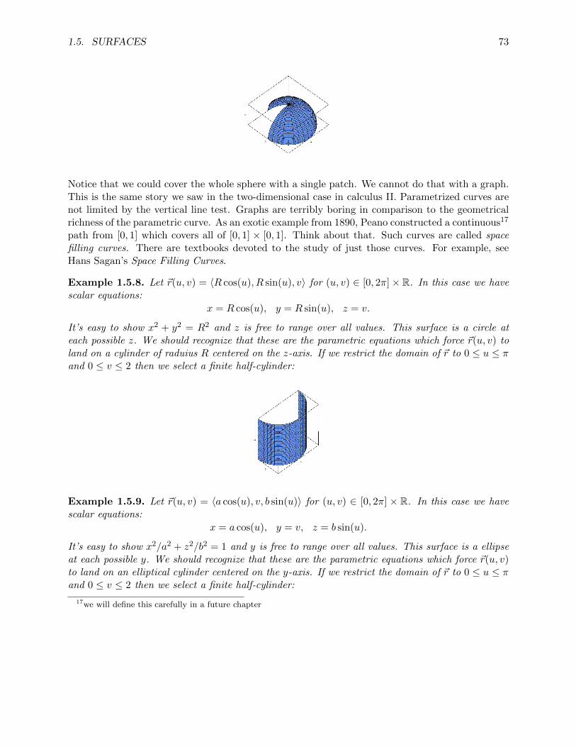
1.5. SURFACES 73
Notice that we could cover the whole sphere with a single patch. We cannot do that with a graph.This is the same story we saw in the two-dimensional case in calculus II. Parametrized curves arenot limited by the vertical line test. Graphs are terribly boring in comparison to the geometricalrichness of the parametric curve. As an exotic example from 1890, Peano constructed a continuous17
path from [0, 1] which covers all of [0, 1] × [0, 1]. Think about that. Such curves are called spacefilling curves. There are textbooks devoted to the study of just those curves. For example, seeHans Sagan’s Space Filling Curves.
Example 1.5.8. Let ~r(u, v) = 〈R cos(u), R sin(u), v〉 for (u, v) ∈ [0, 2π]× R. In this case we havescalar equations:
x = R cos(u), y = R sin(u), z = v.
It’s easy to show x2 + y2 = R2 and z is free to range over all values. This surface is a circle ateach possible z. We should recognize that these are the parametric equations which force ~r(u, v) toland on a cylinder of raduius R centered on the z-axis. If we restrict the domain of ~r to 0 ≤ u ≤ πand 0 ≤ v ≤ 2 then we select a finite half-cylinder:
Example 1.5.9. Let ~r(u, v) = 〈a cos(u), v, b sin(u)〉 for (u, v) ∈ [0, 2π] × R. In this case we havescalar equations:
x = a cos(u), y = v, z = b sin(u).
It’s easy to show x2/a2 + z2/b2 = 1 and y is free to range over all values. This surface is a ellipseat each possible y. We should recognize that these are the parametric equations which force ~r(u, v)to land on an elliptical cylinder centered on the y-axis. If we restrict the domain of ~r to 0 ≤ u ≤ πand 0 ≤ v ≤ 2 then we select a finite half-cylinder:
17we will define this carefully in a future chapter

74 CHAPTER 1. ANALYTIC GEOMETRY
Example 1.5.10. Let ~r(u, v) = 〈R cos(u) sinh(v), R sin(u) sinh(v), R cosh(v)〉 for (u, v) ∈ [0, 2π]×R. In this case we have scalar equations:
x = R cos(u) sinh(v), y = R sin(u) sinh(v), z = R cosh(v).
It’s easy to show −x2− y2 + z2 = R2. If we restrict the domain of ~r to 0 ≤ u ≤ 2π and −2 ≤ v ≤ 2then we select a portion of the upper branch:
The part of the lower branch which is graphed above is covered by the mapping Let ~r(u, v) =〈R cos(u) sinh(v), R sin(u) sinh(v),−R cosh(v)〉 for (u, v) ∈ [0, 2π]× [−2, 2]. The grey shape is wherethe parametrization will cover if we enlarge the domain of the parameterizations.
Example 1.5.11. Let ~r(u, v) = 〈R cosh(u) sin(v), R sinh(u) sin(v), R cos(v)〉 for (u, v) ∈ R×[0, 2π].In this case we have scalar equations:
x = R cosh(u) sin(v), y = R sinh(u) sin(v), z = R cos(v).
It’s easy to show x2− y2 + z2 = R2. I’ve plotted ~r with domain restricted to dom(~r) = [−1.3, 1.3]×[0, π] in blue and dom(~r) = [−1.3, 1.3]×[π, 2π] in green. The grey shape is where the parametrizationwill go if we enlarge the domain.

1.5. SURFACES 75
1.5.3 surfaces as level sets
Unlike curves, we do not need two equations to fix a surface in R 3. In three dimensional space18 ifwe have just one equation in x, y, z that should suffice to leave just two free variables. In a nutshellthat is what a surface is. It is a space which has two degrees of freedom. In the parametric set-upwe declare those freedoms explicitly from the outset by the construction of the patch in terms ofthe parameters. In the level set formulation we focus the attention on an equation which definesthe surface of interest. We already saw this for a plane; the solutions of ax+ by + cz = d fill out aplane with normal 〈a, b, c〉.
Definition 1.5.12. level surface in three dimensional space
Suppose F : dom(F ) ⊆ R 3 → R is a function. Let
S = {(x, y, z) | F (x, y, z) = k}.
We say that S is a level surface of level k with level function F . In other words, S =F−1{k} is a level surface.
A level surface is a fiber of a real-valued function on R 3.
Example 1.5.13. Let F (x, y, z) = a(x − xo) + b(y − yo) + c(z − zo). Recognize that the solutionset of F (x, y, z) = 0 is the plane with base-point (xo, yo, zo) and normal 〈a, b, c〉.
18to pick out a two-dimensional surface in R 4 it would take two equations in t, x, y, z, but, we really only careabout R 3 so, I’ll behave and stick with that case.

76 CHAPTER 1. ANALYTIC GEOMETRY
Example 1.5.14. some level surfaces I can plot without fancy CAS programs:
The example below is not such a case:
Example 1.5.15. This surface has four holes. I have an animation on my website, check it out.
In fact, I don’t think I want to parametrize this beast. Wait, I have students, isn’t this whathomework is for?
Example 1.5.16. Let F (x, y, z) = x2/a2 + y2/b2 + z2/c2. The solution set of F (x, y, z) = 1 iscalled an ellipsoid centered at the origin. In the special case a = b = c = R the ellipsoid is asphere of radius R. Here’s a special case, a = b = c = 1 the unit-sphere:
Example 1.5.17. Let F (x, y, z) = x2+y2−z2. The solution set of F (x, y, z) = 0 is called an conethrough the origin. However, the solution set of F (x, y, z) = k for k 6= 0 forms a hyperboloid of

1.5. SURFACES 77
one-sheet for k > 0 and a hyperboloid of two-sheets for k < 0. The hyperboloids approachthe cone as the distance from the origin grows. I plot a few representative cases:
There is an animation on my webage, take a look.
Some of the examples above fall under the general category of a quadratic surface. Suppose
Q(x, y, z) = ax2 + by2 + cz2 + dxy + exz + fyz + gx+ hy + iz.
For any particular nontrivial selection of constants a, b, . . . , h, i we say the solution of Q(x, y, z) = kis a quadratic surface. For future reference let me list the proper terminology. We’d like to getcomfortable with these terms.
1. a standard ellipsoid is the solution set of x2/a2 + y2/b2 + z2/c2 = 1. If a = b = c then wesay the ellipsoid is a sphere.
2. a standard elliptic paraboloid is the solution set of z/c = x2/a2 + y2/b2. If a = b then wesay the paraboloid is circular.

78 CHAPTER 1. ANALYTIC GEOMETRY
3. a standard hyperbolic paraboloids is the solution set of z/c = y2/b2 − x2/a2.
4. a standard elliptic cone is the solution set of z2/c2 = x2/a2 + y2/b2. If a = b then we saythe cone is circular.
5. a standard hyperboloid of one sheet is the solution set of x2/a2 + y2/b2 − z2/c2 = 1.
6. a standard hyperboloid of two sheets is the solution set of x2/a2 + y2/b2 − z2/c2 = −1.

1.5. SURFACES 79
If you study the formulas above you’ll notice the absense of certain terms in the general quadraticform: terms such as dxy, exz, fyz, gx, hy are absent. Inclusion of these terms will either shift orrotate the standard equations. However, we need linear algebra to properly construct the rotationsfrom the eigenvectors of the quadratic form. I leave that for Math 321 where we have more toys toplay with. You’ll have to be content with the standard examples for the majority of this course.
I’ve inserted the term standard because I don’t mean to say that every elliptic cone has the sameequation as I give. I expect you can translate the standard examples up to an interchange ofcoordinates, that ought not be too hard to understand. For example, y = x2 + 2z2 is clearly anelliptical cone. Or y = x2 − z2 is clearly a hyperbolic paraboloid. Or x2 + z2 − y2 = 1 is clearly ahyperboloid of one sheet whereas −x2 − z2 + y2 = 1 is a hyperboloid of two sheets. These are thepossibilities we ought to anticipate when faced with the level set of some quadratic form. I don’ttry to memorize all of these, I use the method sketched in the next pair of examples. Basically theidea is simply to slice the graph into planes where we find either circles, hyperbolas, lines, ellipsesor perhaps nothing at all. Then we take a few such slices and extrapolate the graph. Often theslices x = 0, y = 0 and z = 0 are very helpful.
Example 1.5.18. .
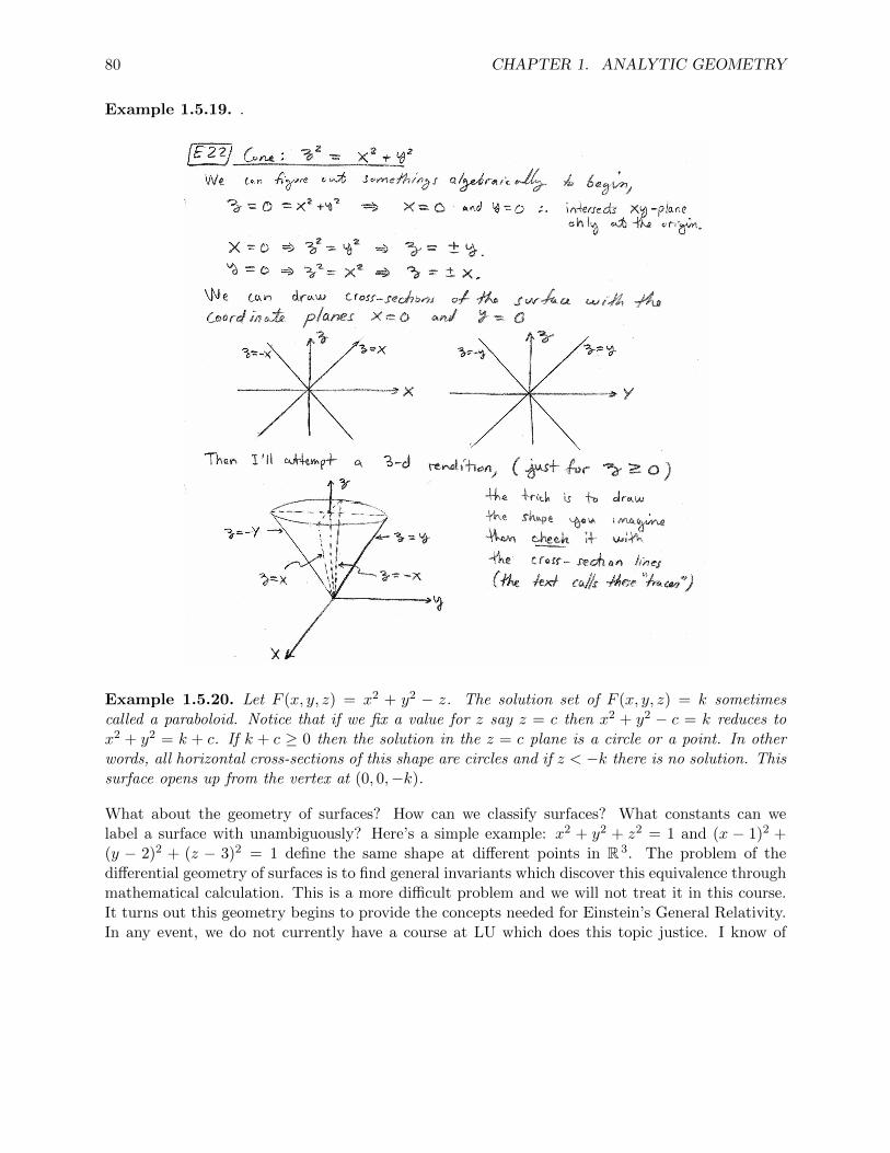
80 CHAPTER 1. ANALYTIC GEOMETRY
Example 1.5.19. .
Example 1.5.20. Let F (x, y, z) = x2 + y2 − z. The solution set of F (x, y, z) = k sometimescalled a paraboloid. Notice that if we fix a value for z say z = c then x2 + y2 − c = k reduces tox2 + y2 = k + c. If k + c ≥ 0 then the solution in the z = c plane is a circle or a point. In otherwords, all horizontal cross-sections of this shape are circles and if z < −k there is no solution. Thissurface opens up from the vertex at (0, 0,−k).
What about the geometry of surfaces? How can we classify surfaces? What constants can welabel a surface with unambiguously? Here’s a simple example: x2 + y2 + z2 = 1 and (x − 1)2 +(y − 2)2 + (z − 3)2 = 1 define the same shape at different points in R 3. The problem of thedifferential geometry of surfaces is to find general invariants which discover this equivalence throughmathematical calculation. This is a more difficult problem and we will not treat it in this course.It turns out this geometry begins to provide the concepts needed for Einstein’s General Relativity.In any event, we do not currently have a course at LU which does this topic justice. I know of
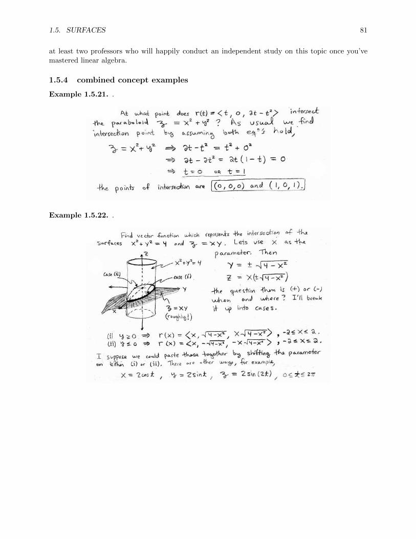
1.5. SURFACES 81
at least two professors who will happily conduct an independent study on this topic once you’vemastered linear algebra.
1.5.4 combined concept examples
Example 1.5.21. .
Example 1.5.22. .

82 CHAPTER 1. ANALYTIC GEOMETRY
Example 1.5.23. .
Example 1.5.24. .
Example 1.5.25. .

1.6. CURVELINEAR COORDINATES 83
1.6 curvelinear coordinates
Cartesian coordinates are a nice starting point, but they make many simple problems needlesslycomplex. If a two-dimensional problem has a quantity which only depends on distance from thecentral point then probably polar coordinates will simplify the equations of the problem. Similarly,if a three dimensional problem possesses a cylindrical symmetry then use cylindrical coordinates.If a three dimensional problem has spherical symmetry then use spherical coordinates.
A coordinate system is called right-handed if the unit-vectors which point in the direction ofincreasing coordinates at each point are related to each other by the right-hand-rule just like thexyz-coordinates. We call this set of unit-vectors the frame of the coordinate system. Generally aframe in Rn is just an assignment of n-vectors at each point in Rn. In linear-algebra langauge, aframe is an assignment of a basis at each point of Rn. Dimensions n = 2 and n = 3 suffice for ourpurposes. If y1, y2, y3 denote coordinates with unit-vectors u1, u2, u3 in the direction of increasingy1, y2, y3 respective then we say the coordinate system is right-handed iff
u1 × u2 = u3, u2 × u3 = u1, u3 × u1 = u2.
In contrast with the constant frame { x, y, z} the frame {u1, u2, u3} is usually point-dependent.An assignment of a vector to each point in some space is called a vector field. A frame is actuallya triple of vector fields which is given over a space. Enough terminology, the equations speak forthemselves soon enough.
1.6.1 polar coordinates
Polar coordinates (r, θ) are defined by
x = r cos θ, y = r sin θ
In quadrants I and IV (regions with x > 0) we also have
r2 = x2 + y2, θ = tan−1[y
x
].
In quadrants II and III (regions with x < 0) we have
r2 = x2 + y2, θ = π + tan−1[y
x
].
Geometrically it is clear that we can label any point in R 2 either by cartesian coordinates (x, y) orby polar coordinates (r, θ). We may view equations in cartesian or polar form.
Example 1.6.1. The circle x2 + y2 = R2 has polar equation r = R.
Typically in the polar context the angle plays the role of the independent variable. In the sameway it is usually customary to write y = f(x) for a graph we try to write r = f(θ).

84 CHAPTER 1. ANALYTIC GEOMETRY
Example 1.6.2. The line y = mx+ b has polar equation r sin θ = mr cos θ + b hence
r =b
sin θ −m cos θ.
Example 1.6.3. The polar equation θ = π/4 translates to y = x for x > 0. The reason is that
π
4= tan−1
[y
x
]⇒ tan
π
4=y
x⇒ 1 =
y
x⇒ y = x
and the ray with θ = π/4 is found in quadrant I where x > 0.
Let us denote unit vectors in the direction of increasing r, θ by r, θ respective. You can derive bygeometry alone that
r = cos(θ) x+ sin(θ) y
θ = − sin(θ) x+ cos(θ) y.(1.5)
We call {r, θ} the frame of polar coordinates. Notice that these are perpendicular at each point;r • θ = 0.
Example 1.6.4. If we want to assign a vector to each point on the unit circle such that the vectoris tangent and pointing in the counter-clockwise (CCW) direction then a natural choice is θ.
Example 1.6.5. If we want to assign a vector to each point on the unit circle such that the vectoris pointing radially out from the center then a natural choice is r.
Suppose you have a perfectly flat floor and you pour paint slowly in a perfect even stream then inprinciple you’d expect it would spread out on the floor in the r direction if we take the spill spotas the origin and the floor as the xy-plane.
1.6.2 cylindrical coordinates
Cylindrical coordinates (r, θ, z) are defined by
x = r cos θ, y = r sin θ, z = z
In quadrants I and IV (regions with x > 0) we also have
r2 = x2 + y2, θ = tan−1[y
x
].

1.6. CURVELINEAR COORDINATES 85
In quadrants II and III (regions with x < 0) we have
r2 = x2 + y2, θ = π + tan−1[y
x
].
Geometrically it is clear that we can label any point in R 3 either by cartesian coordinates (x, y, z)or by cylindrical coordinates (r, θ, z).
We may view equations in cartesian or cylindrical form.
Example 1.6.6. In cylindrical coordinates the equation r = 1 is a cylinder since the z-variable isfree. If we denote the unit-circle by S1 = {(x, y) | x2 + y2 = 1} then the solution set of r = 1 hasthe form S1 × R. At each z we get a copy of the circle S1.
Example 1.6.7. The equation θ = π/4 is a half-plane which has equation y = x subject to thecondition x > 0.
Let us denote unit vectors in the direction of increasing r, θ, z by r, θ, z respectively. You canderive by geometry alone that
r = cos(θ) x+ sin(θ) y
θ = − sin(θ) x+ cos(θ) yz = 〈0, 0, 1〉.
(1.6)
We call {r, θ, z} the unit-frame of cylindrical coordinates.

86 CHAPTER 1. ANALYTIC GEOMETRY
Example 1.6.8. Suppose we have a line of electric charge smeared along the z-axis with chargedensity λ. One can easily derive from Gauss’ Law that the electric field has the form:
~E =λ
2πεorr.
Example 1.6.9. If we have a uniform current I z flowing along the z-axis then the magnetic fieldcan be derived from Ampere’s Law and has the simple form:
~B =µoI
2πrθ
Trust me when I tell you that the formulas in terms of cartesian coordinates are not nearly as clean.
If we fix our attention to a particular point the cylindrical frame has the same structure as thecartesian fram { x, y, z}. In particular, we can show that
r • r = 1, θ • θ = 1, z • z = 1
θ • r = 0, θ • z = 0, z • r = 0.
We can also calculate either algebraically or geometrically that:
r × θ = z, θ × z = r, z × r = θ
Therefore, the cylindrical coordinate system (r, θ, z) is a right-handed coordinate system sinceit provides a right-handed basis of unit-vectors at each point. We can summarize these relationscompactly with the notation u1 = r, u2 = θ, u3 = z whence:
ui • uj = δij , ui × uj =3∑
k=1
εijkuk
this is the same pattern we saw for the cartesian unit vectors.

1.6. CURVELINEAR COORDINATES 87
1.6.3 spherical coordinates
Spherical coordinates19 (ρ, φ, θ) relate to Cartesian coordinates as follows
x = ρ cos(θ) sin(φ)y = ρ sin(θ) sin(φ)z = ρ cos(φ)
(1.7)
where ρ > 0 and 0 ≤ φ ≤ π and 0 ≤ θ ≤ 2π. We can derive,
ρ2 = x2 + y2 + z2
tan(φ) =√x2 + y2/z
tan(θ) = y/x.
(1.8)
It is clear that any point in R 3 is labeled both by cartesian coordinates (x, y, z) or sphericalcoordinates (ρ, φ, θ).
Also, it is important to distinguish between the geometry of the polar angle θ and the azmuthialangle φ
19I’ll use notation which is consistent with Stewart, but beware there is a better notation used in physics andengineering where the meaning of φ and θ are switched and the spherical radius ρ is instead denoted by r
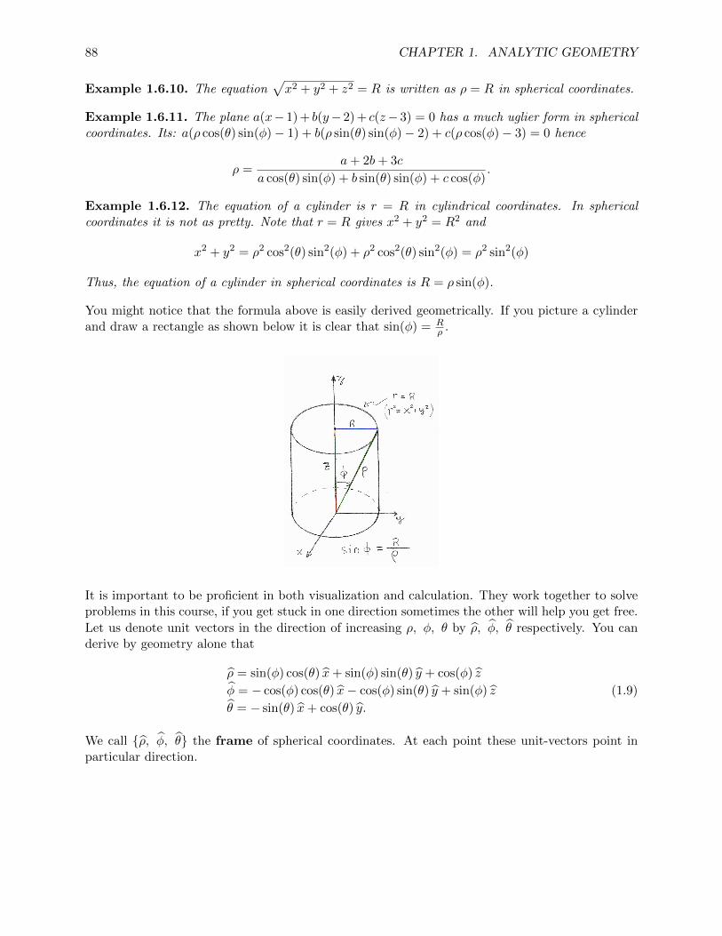
88 CHAPTER 1. ANALYTIC GEOMETRY
Example 1.6.10. The equation√x2 + y2 + z2 = R is written as ρ = R in spherical coordinates.
Example 1.6.11. The plane a(x− 1) + b(y− 2) + c(z− 3) = 0 has a much uglier form in sphericalcoordinates. Its: a(ρ cos(θ) sin(φ)− 1) + b(ρ sin(θ) sin(φ)− 2) + c(ρ cos(φ)− 3) = 0 hence
ρ =a+ 2b+ 3c
a cos(θ) sin(φ) + b sin(θ) sin(φ) + c cos(φ).
Example 1.6.12. The equation of a cylinder is r = R in cylindrical coordinates. In sphericalcoordinates it is not as pretty. Note that r = R gives x2 + y2 = R2 and
x2 + y2 = ρ2 cos2(θ) sin2(φ) + ρ2 cos2(θ) sin2(φ) = ρ2 sin2(φ)
Thus, the equation of a cylinder in spherical coordinates is R = ρ sin(φ).
You might notice that the formula above is easily derived geometrically. If you picture a cylinderand draw a rectangle as shown below it is clear that sin(φ) = R
ρ .
It is important to be proficient in both visualization and calculation. They work together to solveproblems in this course, if you get stuck in one direction sometimes the other will help you get free.
Let us denote unit vectors in the direction of increasing ρ, φ, θ by ρ, φ, θ respectively. You canderive by geometry alone that
ρ = sin(φ) cos(θ) x+ sin(φ) sin(θ) y + cos(φ) z
φ = − cos(φ) cos(θ) x− cos(φ) sin(θ) y + sin(φ) z
θ = − sin(θ) x+ cos(θ) y.
(1.9)
We call {ρ, φ, θ} the frame of spherical coordinates. At each point these unit-vectors point inparticular direction.

1.6. CURVELINEAR COORDINATES 89
In constrast to the cartesian frame which is constant20 over all of R 3.
Example 1.6.13. Suppose we a point charge q is placed at the origin then by Gauss’ Law we canderive
~E =q
4πεoρ2ρ.
This formula makes manifest the spherical direction of the electric field, the absence of the angularunit-vectors says the field has no angular dependence and hence its values depend only on thespherical radius ρ. This is called the Coulomb field or monopole field. Almost the same mathapplies to gravity. If M is placed at the origin then
~F =GmM
ρ2(−ρ).
gives the gravitational force ~F of M on m at distance ρ from the origin. The direction of thegravitational field is −ρ which simply says the field points radially inward.
The spherical frame gives us a basis of vectors to build vectors at each point in R 3. More thanthat, the spherical frame is an orthonormal frame since at any particular point the frame providesan orthonormal set of vectors. In particular, we can show that
ρ • ρ = 1, φ • φ = 1, θ • θ = 1
φ • ρ = 0, θ • ρ = 0, φ • θ = 0.
We can also calculate either algebraically or geometrically that:
θ × ρ = φ, ρ× φ = θ, φ× θ = ρ
20How do I know the cartesian frame is unchanging? It’s not complicated really; x = 〈1, 0, 0〉, y = 〈0, 1, 0〉 andz = 〈0, 0, 1〉.
90 CHAPTER 1. ANALYTIC GEOMETRY
Therefore, the spherical coordinate system (ρ, φ, θ) is a right-handed coordinate system since itprovides a right-handed basis of unit-vectors at each point. We can summarize these relationscompactly with the notation u1 = ρ, u2 = φ, u3 = θ whence:
ui • uj = δij , ui × uj =3∑
k=1
εijkuk
this is the same pattern we saw for the cartesian unit vectors.
We will return to the polar, cylindrical and spherical coordinate systems as the course progresses.Even now we could consider a multitude of problems based on the combination of the material cov-ered thus-far and it’s intersection with curvelinear coordinates. There are other curved coordinatesystems beyond these standard three, but I leave those to your imagination for the time being. I dodiscuss a more general concept of coordinate system in the advanced calculus course. In manifoldtheory the concept of a coordinate system is refined in considerable depth. We have no need ofsuch abstraction here so I’ll behave21.
21I’d guess most calculus text editors would say this whole paragraph is misbehaving, but I have no editor so ha.