multirate digital signal...
TRANSCRIPT
Multirate Digital SignalProcessing

2
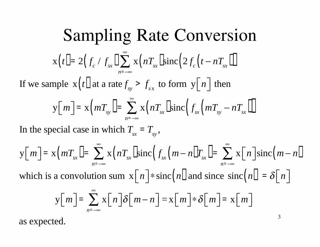
Sampling Rate ConversionIf a digital signal is formed by properly sampling an analog signal, it is possible in principle, to convert it back to analogform and re-sample it at a new sampling rate. But it would bebetter to directly change from one sampling rate to another without going through the analog form.
If a signal x n is formed by properly sampling x t( ) then
x t( ) = 2 fc
/ fsx( ) x n sinc 2 f
ct nT
sx( )( )n=
where fc is the corner frequency of a filter with impulse response
h t( ) = 2 fcT
sxsinc 2 f
ct( ) F
H f( ) = Tsx
1 , 0 < f < fc
0 , otherwise
3
Sampling Rate Conversion
x t( ) = 2 fc
/ fsx( ) x nT
sx( )sinc 2 fc
t nTsx( )( )
n=
If we sample x t( ) at a rate fsy
> fs x
to form y n then
y m = x mTsy( ) = x nT
sx( )sinc fsx
mTsy
nTsx( )( )
n=
In the special case in which Tsx
= Tsy
,
y m = x mTsx( ) = x nT
sx( )sinc fsx
m n( )Tsx( )n=
= x n sinc m n( )n=
which is a convolution sum x n sinc n( ) and since sinc n( ) = n
y m = x n m nn=
= x m m = x m
as expected.

4
Sampling Rate Conversion
In the general case Tsx
Tsy
,
y m = x nTsx( )sinc f
sxmT
synT
sx( )( )n=
, fsy
> fsx
or
y m = x nTsx( )sinc mT
sy/ T
sxn( )
n=
, fsy
> fsx
Now let mTsy
/ Tsx
= km
+m
where km
= mTsy
/ Tsx
and m
= mTsx
/ Tsy
km. Then
y m = x nTsx( )sinc k
m+
mn( )
n=
, fsy
> fsx
5
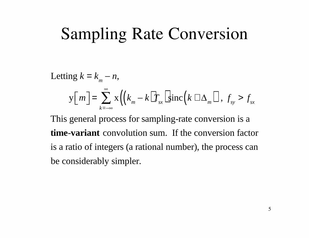
Sampling Rate Conversion
Letting k = km
n,
y m = x km
k( )Tsx( )sinc k +m( )
k=
, fsy
> fsx
This general process for sampling-rate conversion is a
time-variant convolution sum. If the conversion factor
is a ratio of integers (a rational number), the process can
be considerably simpler.

6
Sampling Rate ConversionDownsampling by a factor D
Sample a signal x n by multiplying
it by a periodic impulse
Dn = n mD
m=
to produce xs
n = x nD
n .
D = 4
7
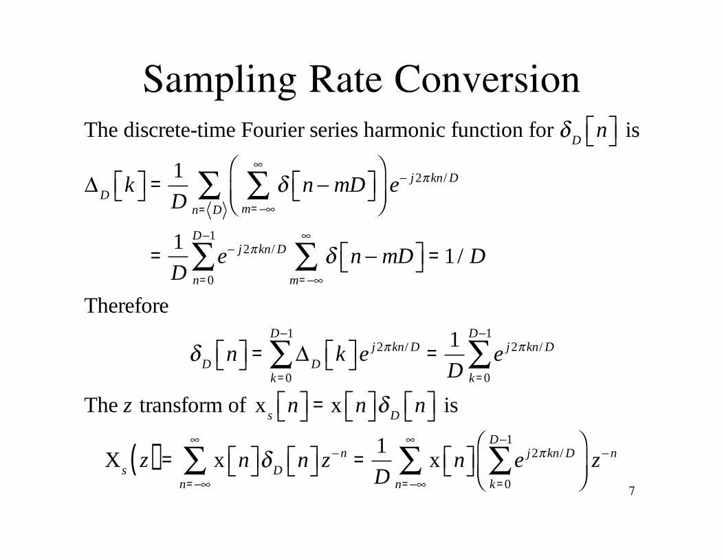
Sampling Rate Conversion
The discrete-time Fourier series harmonic function for D
n is
Dk =
1
Dn mD
m=
e j2 kn/ D
n= D
=1
De j2 kn/ D n mD
m=n=0
D 1
= 1/ D
Therefore
D
n =D
k e j2 kn/ D
k=0
D 1
=1
De j2 kn/ D
k=0
D 1
The z transform of xs
n = x nD
n is
Xs
z( ) = x nD
n z n
n=
=1
Dx n e j2 kn/ D
k=0
D 1
z n
n=

8
Sampling Rate Conversion
Xs
z( ) =1
Dx n e j2 kn/ Dz n
n=
=1
Dx n e j2 k / Dz 1( )
n
n=k=0
D 1
k=0
D 1
=1
DX ze j2 k / D( )
k=0
D 1
Xs
e j( ) =1
DX e j e j2 k / D( )
k=0
D 1
=1
DX e
j 2 k / D( )( )k=0
D 1

9
Sampling Rate Conversion
To reduce the number of samples, decimate the sampled signal
to form xd
n = xs
Dn . The z transform of xd
n is
Xd
z( ) = xd
n z n
n=
= xs
Dn z n
n=
. Let m = Dn.
Then Xd
z( ) = xs
m z m/ D
m=m/ D aninteger
= xs
m z m/ D
m=
= Xs
z1/ D( )
because all values of xs
m for m / D not an integer are zero( )
Combining this result with Xs
z( ) =1
DX ze j2 k / D( )
k=0
D 1
we get
Xd
z( ) =1
DX z1/ De j2 k / D( )
k=0
D 1
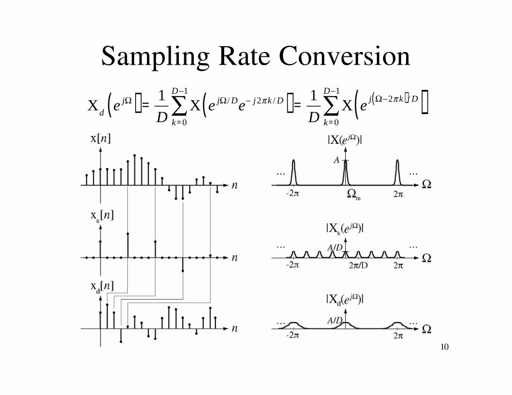
10
Sampling Rate Conversion
X
de j( ) =
1
DX e j / De j2 k / D( )
k=0
D 1
=1
DX e
j 2 k( )/ D( )k=0
D 1
11
Sampling Rate Conversion
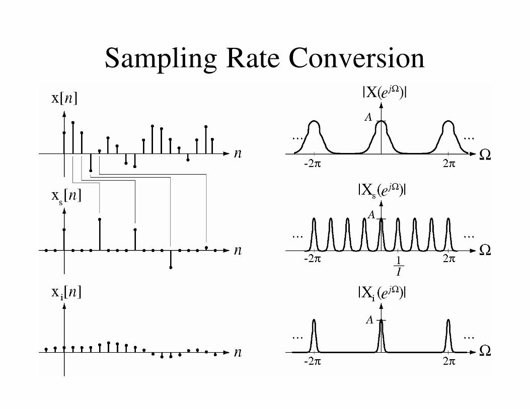
The opposite of downsampling is upsampling. If the original
signal is x n the upsampled signal is
xs
n =x n / I , n / I an integer
0 , otherwise

12
Sampling Rate Conversion
A discrete-time expansion by a factor of I corresponds to a
discrete-time-frequency compression by the same factor.
Xs
z( ) = X zI( ) X
se
j( ) = X ejI( )

13
Sampling Rate Conversion
An ideal lowpass filter with transfer function
H e j( ) = rect I 2 k( ) / 2( )k=
=1 , < / I
0 , / I < <
could be used to interpolate between sample values yielding
Xi
e j( ) = Xs
e j( ) rect I 2 k( ) / 2( )k=
which corresponds to xi
n = xs
n 1/ I( )sinc n / I( ) in the
time domain.
14
Sampling Rate Conversion

15
Polyphase Filters
The polyphase filter was developed for the efficient
implementation of sampling rate conversion. Any transfer
function is of the form
H z( ) = + h 0 + z1 h 1 + + z
k h k +
which can be regrouped and written as
H z( ) = + h 0 + zM h M +
z-1h 1 + z
M +1( )h M +1 +
z- M -1( )
h M -1 + z2 M 1( )
h 2M 1 +

16
Polyphase Filters
H z( ) = + h 0 + zM h M +
z-1 h 1 + z
M h M +1( ) +
z- M -1( )
h M -1 + zM h 2M 1( ) +
This can be written compactly as
H z( ) = z1 P
iz
M( )i=0
M 1
where Pi
z( ) = h nM + i( ) zn
n=
This is called the “M-component polyphase decomposition” of H z( )and the P
iz( ) 's are the polyphase components of H z( ).

17
Polyphase Filters

18
The Noble Identities
The relationships between a signal and a decimated version of
the signal was found to be X e j( ) = D Xd
e jD( ) , 0 < < / D.
It then follows that, in the z domain,
X z( ) = D Xd
z D( ) and Xd
z( ) = 1/ D( )X z1/ D( )for signals sampled according to the sampling theorem.
Consider a downsampler followed by a filter with input signal
x n and output signal y n and let the downsampler output
be y1
n .

19
The Noble Identities
Y1
z( ) = 1/ D( )X z1/ D( ) and Y z( ) = H z( )Y
1z( )
Therefore Y z( ) = 1/ D( )H z( )X z1/ D( ).
Now reverse the order of the downsampler and filter.
Y1
z( ) = H z( )X z( ) and Y z( ) = 1/ D( )Y1
z1/ D( )
Therefore Y z( ) = 1/ D( )H z1/ D( )X z
1/ D( ).The two output signals are not the same because the
downsampler is not an LTI system. But they would
be the same if z zD in H z( ) in the second system.

20
The Noble IdentitiesFor decimators
For interpolators
21
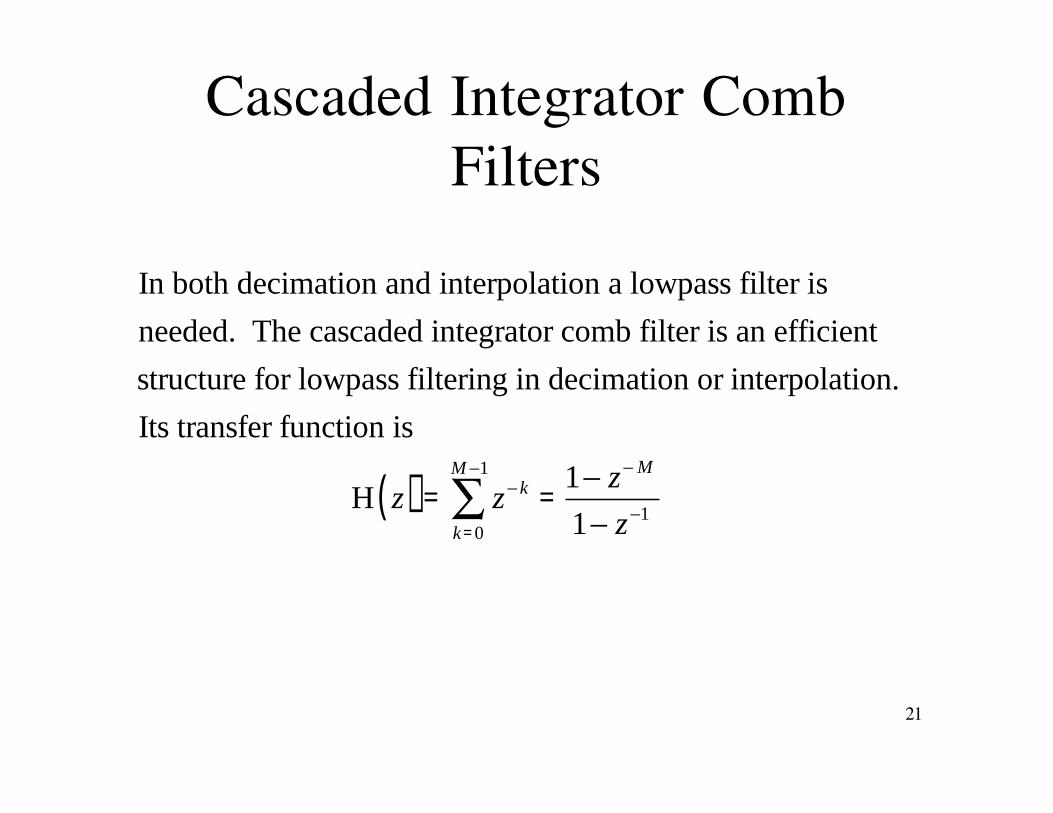
Cascaded Integrator CombFilters
In both decimation and interpolation a lowpass filter is
needed. The cascaded integrator comb filter is an efficient
structure for lowpass filtering in decimation or interpolation.
Its transfer function is
H z( ) = zk
k=0
M 1
=1 z
M
1 z1

22
Cascaded Integrator CombFilters
In decimation
In interpolation
23
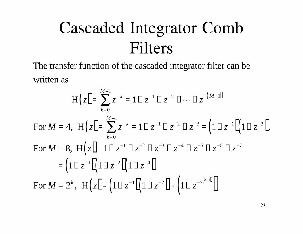
Cascaded Integrator CombFilters
The transfer function of the cascaded integrator filter can be
written as
H z( ) = zk
k=0
M 1
= 1+ z1+ z
2+ + z
M 1( )
For M = 4, H z( ) = zk
k=0
M 1
= 1+ z1+ z
2+ z
3= 1+ z
1( ) 1+ z2( ).
For M = 8, H z( ) = 1+ z1+ z
2+ z
3+ z
4+ z
5+ z
6+ z
7
= 1+ z1( ) 1+ z
2( ) 1+ z4( )
For M = 2k , H z( ) = 1+ z1( ) 1+ z
2( ) 1+ z2
k 1( )
( )

24
Cascaded Integrator CombFilters
H z( ) = 1+ z
1( ) 1+ z2( ) 1+ z
2k 1( )
( )

25
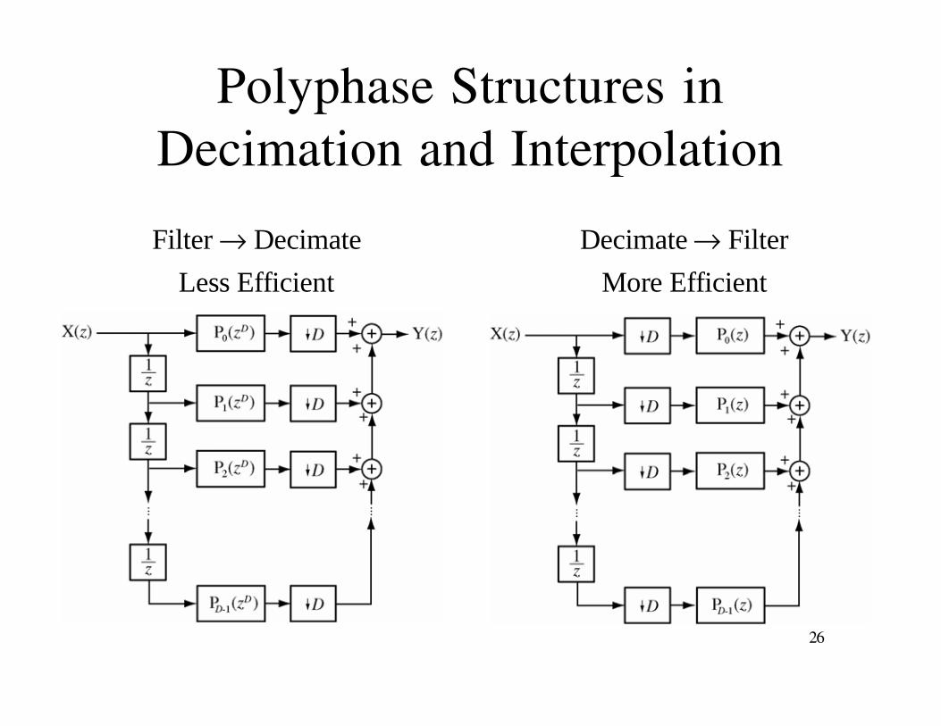
Polyphase Structures inDecimation and Interpolation
The basic decimator model is a lowpass filter followed bya downsampler.
One inefficiency is that the filtering computations are doneat the higher sampling rate but the results are only neededat the lower sampling rate. We can improve the efficiencyby using a polyphase structure.
26
Polyphase Structures inDecimation and Interpolation
Filter Decimate
Less Efficient
Decimate Filter
More Efficient
27
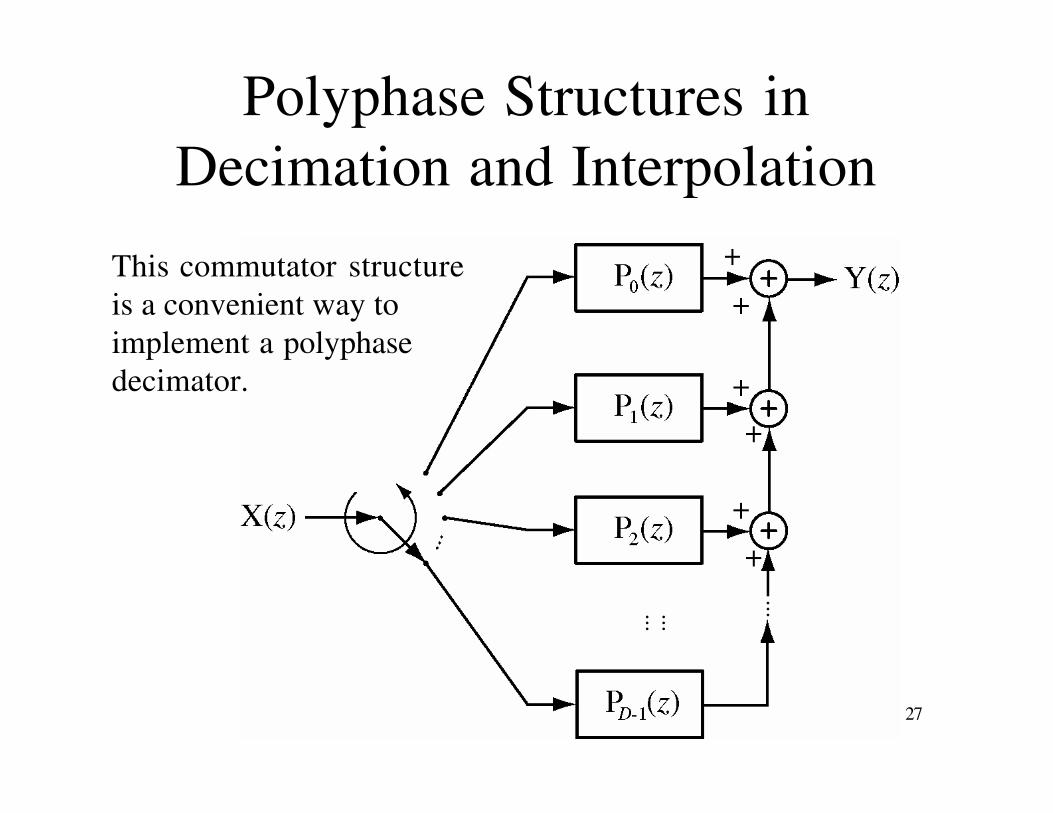
Polyphase Structures inDecimation and Interpolation
This commutator structureis a convenient way to implement a polyphasedecimator.

28
Polyphase Structures inDecimation and Interpolation
Interpolate Filter
Less Efficient
Filter Interpolate
More Efficient
29
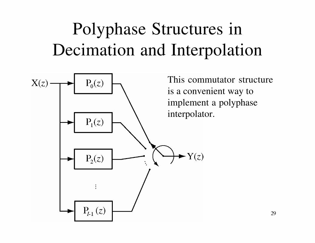
Polyphase Structures inDecimation and Interpolation
This commutator structureis a convenient way to implement a polyphaseinterpolator.
30
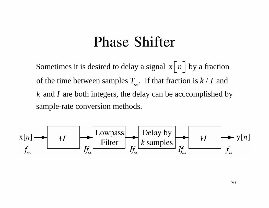
Phase Shifter
Sometimes it is desired to delay a signal x n by a fraction
of the time between samples Tsx
. If that fraction is k / I and
k and I are both integers, the delay can be acccomplished by
sample-rate conversion methods.
31
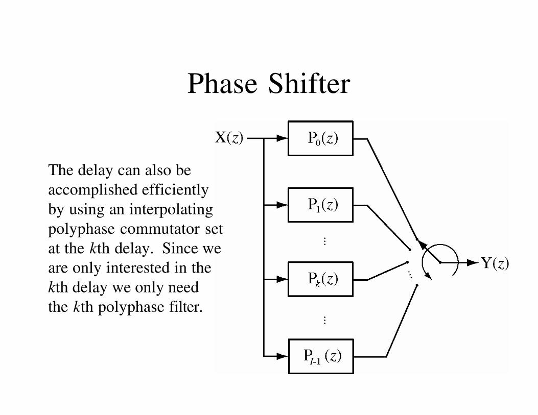
Phase Shifter
The delay can also be accomplished efficiently by using an interpolatingpolyphase commutator set at the kth delay. Since we are only interested in the kth delay we only need the kth polyphase filter.
32
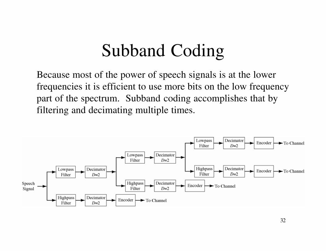
Subband CodingBecause most of the power of speech signals is at the lowerfrequencies it is efficient to use more bits on the low frequencypart of the spectrum. Subband coding accomplishes that byfiltering and decimating multiple times.

33
Subband Coding
The speech signal can be recovered by doing the opposite ofsubband coding.

34
Digital Filter Banks
An important type of analysis
filter bank is the DFT filter
bank. Let the lowpass filters
have impulse responses
h n[ ] = n m[ ]m=0
N 1
and
frequency response
H e j( ) = e j N 1( )/2 sin N / 2( )sin / 2( )

35
Digital Filter Banks
H e j( ) = e j N 1( )/2 sin N / 2( )sin / 2( )

36
Digital Filter BanksThe output signal from the kth filter would be
Yk e j( ) = X e j( ) 2 k / N( )( )e j N 1( )/2 sin N / 2( )sin / 2( )
Yk e j( ) = X e j 2 k / N( )( )e j N 1( )/2 sin N / 2( )sin / 2( )
or, in the time domain
yk n[ ] = x n[ ]e j2 kn / N( ) h n[ ] = x n m[ ]e j2 k n m( )/ N
m=n N 1( )
n
yk N 1[ ] = x q[ ]e j2 kq / N
q=0
N 1
which, at any time n, is X k[ ]
the kth harmonic value in the DFT of the last N values of n.

37
Digital Filter Banks
Since the filters are lowpass, the output signals can be
decimated by N . Without decimation they are
yk n[ ] = x n[ ]e j2 kn / N( ) h0 n[ ] = h0 n m[ ]x m[ ]e j2 km / N
m=n N 1( )
n
and with decimation they are
Xk m[ ] = h0 mN n[ ]x n[ ]e j2 kn / N
n=m N 1( )
m
where m is the discrete time at the output which is not the
same as n the discrete time at the input.

38
Digital Filter Banks
An analysis filterbank with decimation.
39
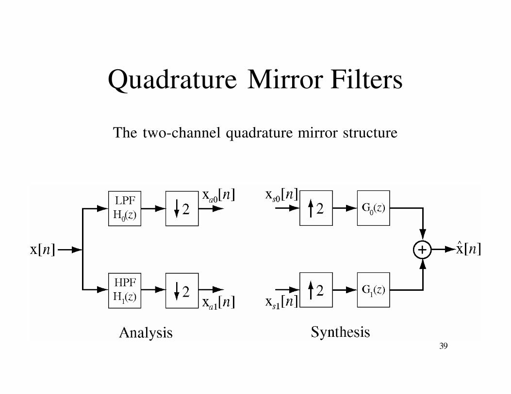
Quadrature Mirror Filters
The two-channel quadrature mirror structure

40
Quadrature Mirror FiltersThe Fourier transforms of the output signals from the analysis
section are
Xa0 e j( ) =1
2X e j /2( )H0 e j /2( ) + X e j 2( )/2( )H0 e j 2( )/2( )
and
Xa1 e j( ) =1
2X e j /2( )H1 e j /2( ) + X e j 2( )/2( )H1 e j 2( )/2( )
The Fourier transform of the output signal from the synthesis section is
X̂ e j( ) = Xs0 e j2( )G0 e j( ) + Xs1 e j2( )G1 e j( )
41
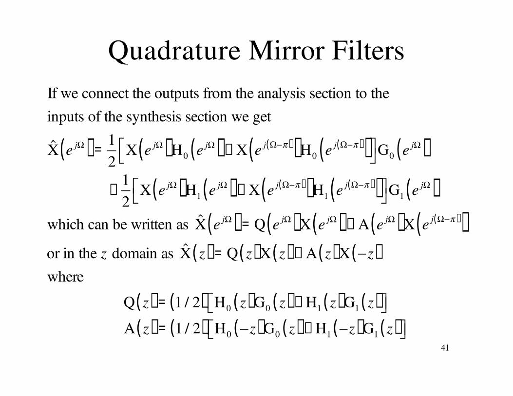
Quadrature Mirror FiltersIf we connect the outputs from the analysis section to the
inputs of the synthesis section we get
X̂ e j( ) =1
2X e j( )H0 e j( ) + X e j( )( )H0 e j( )( ) G0 e j( )
+1
2X e j( )H1 e j( ) + X e j( )( )H1 e j( )( ) G1 e j( )
which can be written as X̂ e j( ) = Q e j( )X e j( ) + A e j( )X e j( )( )or in the z domain as X̂ z( ) = Q z( )X z( ) + A z( )X z( )
where
Q z( ) = 1 / 2( ) H0 z( )G0 z( ) + H1 z( )G1 z( )
A z( ) = 1 / 2( ) H0 z( )G0 z( ) + H1 z( )G1 z( )

42
Quadrature Mirror Filters
The second term A z( )X z( ) is an undesirable alias. If we
set A z( ) = 0 we get
H0 z( )G0 z( ) + H1 z( )G1 z( ) = 0
H0 e j( )( )G0 e j( ) = H1 e j( )( )G1 e j( )Then if we set
G0 e j( ) = H1 e j( )( ) and G1 e j( ) = H0 e j( )( )we get
H0 e j( )( )H1 e j( )( ) = H1 e j( )( )H0 e j( )( )and A z( ) = 0.
43
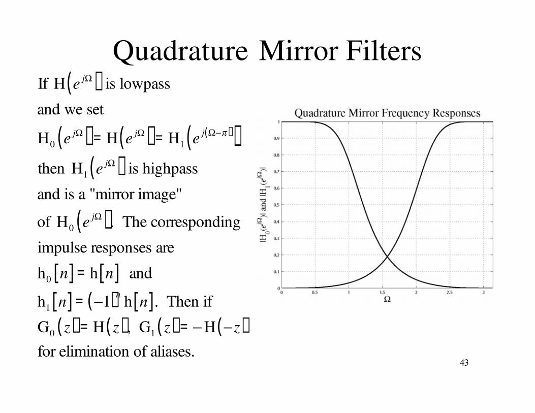
Quadrature Mirror FiltersIf H e j( ) is lowpass
and we set
H0 e j( ) = H e j( ) = H1 e j( )( )then H1 e j( ) is highpass
and is a "mirror image"
of H0 e j( ). The corresponding
impulse responses are
h0 n[ ] = h n[ ] and
h1 n[ ] = 1( )n
h n[ ]. Then if
G0 z( ) = H z( ), G1 z( ) = H z( )
for elimination of aliases.
44
Quadrature Mirror Filters
In summary, for elimination of aliases
H0 z( ) = H z( )
H1 z( ) = H z( )
G0 z( ) = H z( )
G1 z( ) = H z( )
45
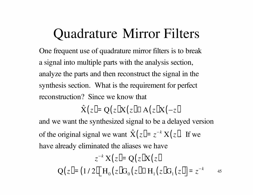
Quadrature Mirror FiltersOne frequent use of quadrature mirror filters is to break
a signal into multiple parts with the analysis section,
analyze the parts and then reconstruct the signal in the
synthesis section. What is the requirement for perfect
reconstruction? Since we know that
X̂ z( ) = Q z( )X z( ) + A z( )X z( )
and we want the synthesized signal to be a delayed version
of the original signal we want X̂ z( ) = z k X z( ). If we
have already eliminated the aliases we have
z k X z( ) = Q z( )X z( )
Q z( ) = 1 / 2( ) H0 z( )G0 z( ) + H1 z( )G1 z( ) = z k
46
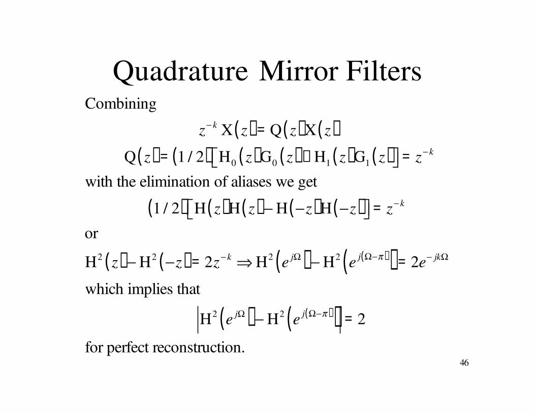
Quadrature Mirror FiltersCombining
z k X z( ) = Q z( )X z( )
Q z( ) = 1 / 2( ) H0 z( )G0 z( ) + H1 z( )G1 z( ) = z k
with the elimination of aliases we get
1 / 2( ) H z( )H z( ) H z( )H z( ) = z k
or
H2 z( ) H2 z( ) = 2z k H2 e j( ) H2 e j( )( ) = 2e jk
which implies that
H2 e j( ) H2 e j( )( ) = 2
for perfect reconstruction.

47
Polyphase Quadrature MirrorFilters
Let
H0 z( ) = P0 z2( ) + z 1P1 z2( ) H1 z( ) = P0 z2( ) z 1P1 z2( )Then
G0 z( ) = P0 z2( ) + z 1P1 z2( )
G1 z( ) = P0 z2( ) z 1P1 z2( )
48
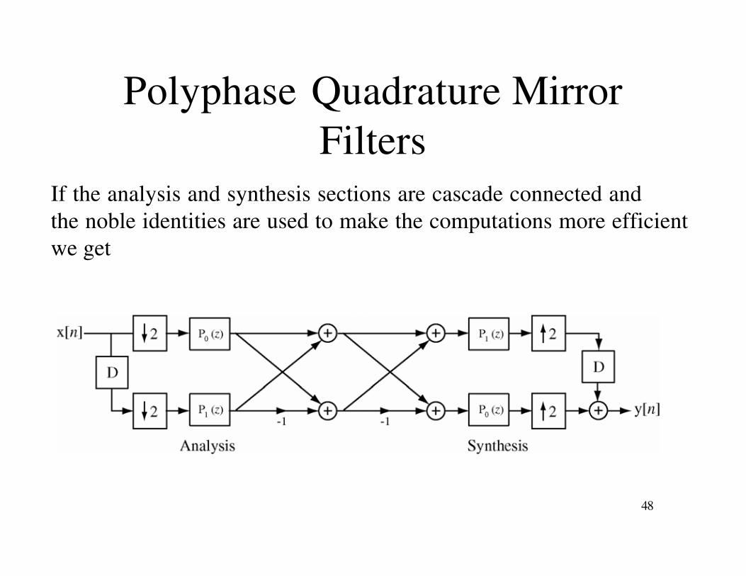
If the analysis and synthesis sections are cascade connected and the noble identities are used to make the computations more efficient we get
Polyphase Quadrature MirrorFilters

49
Perfect Reconstruction QMF
Perfect reconstruction of the input signal can be acheived by
an FIR half-band filter of length 2N 1. A half-band filter
is a zero-phase FIR filter whose impulse response b n[ ] satisfies
b 2n[ ] =constant , n = 0
0 , n 0
If it is zero-phase then b n[ ] = b n[ ]. The frequency response
is B e j( ) = b n[ ]e j n
n= K
K
where K is odd.

50
Perfect Reconstruction QMF
B e j( ) = b n[ ]e j n
n= K
K
= b 0[ ]+ 2 b n[ ]cos n( )n=1n odd
K
B e j( ) = b 0[ ]+ 2 b 2n +1[ ]cos 2n +1( )( )n=0
K 1( )/2
B e j( ) = b 0[ ]+ 2 b 1[ ]cos( ) + b 3[ ]cos 3( ) + + b K[ ]cos K( ){ }
B e j( )( ) = b 0[ ] 2 b 1[ ]cos( ) + b 3[ ]cos 3( ) + + b K[ ]cos K( ){ }
B e j( ) + B e j( )( ) = 2b 0[ ] a constant for all .

51
Perfect Reconstruction QMF
As an example let
b n[ ] =
,0,0, 1 / 7,0,1 / 5,0, 1 / 3,0,1,
2,1,0, 1 / 3,0,1 / 5,0, 1 / 7,0,0,
Then
B e j( ) =2
+ 2 cos( ) + cos 3( ) / 3 + cos 5( ) / 5{ }

52
Perfect Reconstruction QMF
The filter with impulse response b n[ ] is non-causal. It can be
made causal by delaying it by K samples. Also the frequency
response B e j( ) goes negative at some frequencies. If we add
a term B just large enough to make it non-negative at all
frequencies we get B+ e j( ) = B e j( ) + B . Since it is non-negative
it is possible to write it in the form
B+ e j( ) = H e j( )2
= H e j( )H e j( )
Since h n[ ] h n[ ] F H e j( )H e j( ) we can say that
the corresponding impulse response has a length N if b n[ ]has length 2N 1.

53
Perfect Reconstruction QMF
Now delay the original impulse response by N 1 samples
to make it causal and redefine it as
B+ e j( ) = H e j( )2e j N 1( )
= H e j( )H e j( )e j N 1( )
Using the fact that
B e j( ) = b 0[ ]+ 2b 1[ ]cos( ) + b 3[ ]cos 3( ) +
+ b K[ ]cos K( )
it follows that
B+ e j( ) = b 0[ ]+ 2b 1[ ]cos( ) + b 3[ ]cos 3( ) +
+ b K[ ]cos K( )+ B e j N 1( )
54
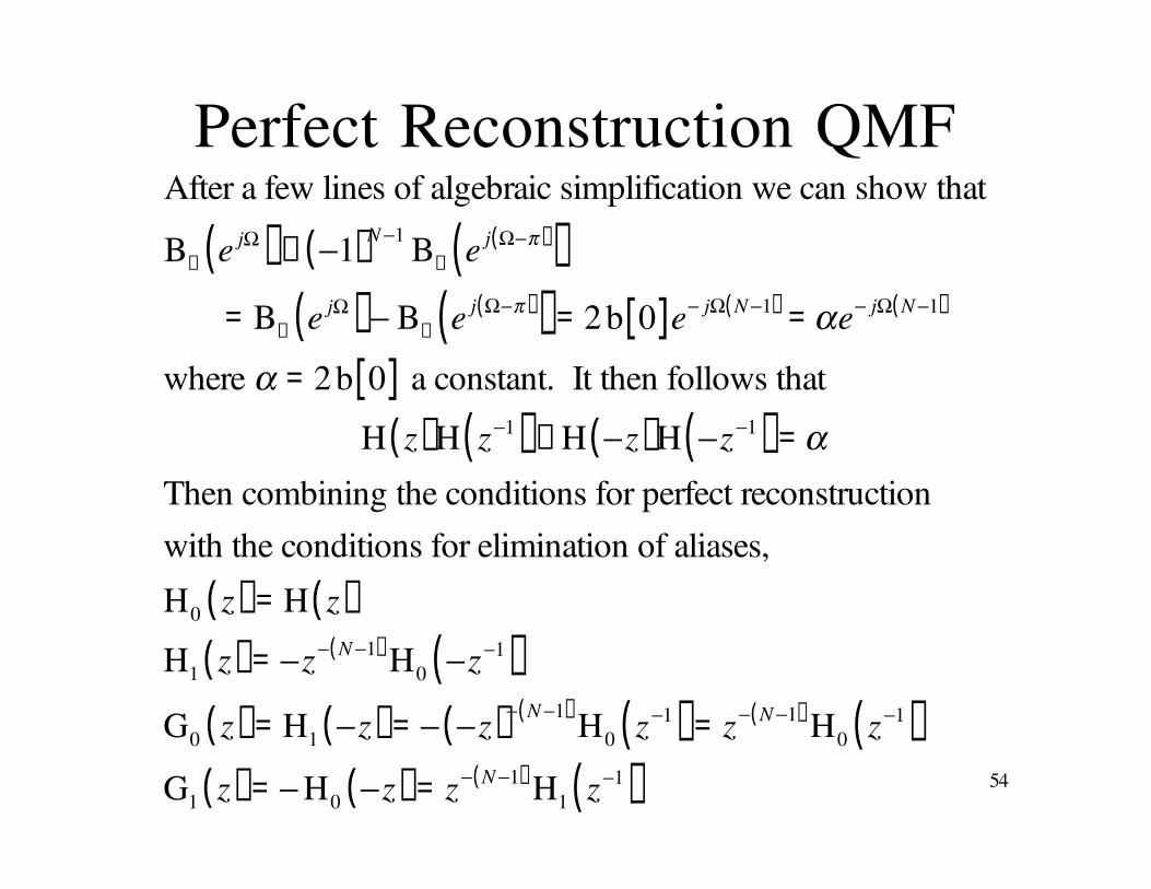
Perfect Reconstruction QMFAfter a few lines of algebraic simplification we can show that
B+ e j( ) + 1( )N 1
B+ e j( )( ) = B+ e j( ) B+ e j( )( ) = 2 b 0[ ]e j N 1( )
= e j N 1( )
where = 2b 0[ ] a constant. It then follows that
H z( )H z 1( ) + H z( )H z 1( ) =
Then combining the conditions for perfect reconstruction
with the conditions for elimination of aliases,
H0 z( ) = H z( )
H1 z( ) = z N 1( ) H0 z 1( )
G0 z( ) = H1 z( ) = z( )N 1( ) H0 z 1( ) = z N 1( ) H0 z 1( )
G1 z( ) = H0 z( ) = z N 1( ) H1 z 1( )

55
Perfect Reconstruction QMFAs an example let H0 z( ) = 1 / 2( ) 1+ z 1( ).Then the four filters in the perfect reconstruction QMF
analysis structure are
H0 z( ) = 1 / 2( ) 1+ z 1( ) H1 z( ) = 1 / 2( ) 1 z 1( )
G0 z( ) = 1 / 2( ) 1+ z 1( ) G1 z( ) = 1 / 2( ) 1 z 1( )

56
Perfect Reconstruction QMF
The four impulse responses are
h0 n[ ] = 1 / 2( ) n[ ]+ n 1[ ]( )
h1 n[ ] = 1 / 2( ) n[ ] n 1[ ]( )
g0 n[ ] = 1 / 2( ) n[ ]+ n 1[ ]( )
g1 n[ ] = 1 / 2( ) n[ ] n 1[ ]( )and the response to a random
excitation is a perfect reconstruction
except delayed and multiplied by two.