Multiproduct Firms and Price-Setting:

Theory and Evidence from U.S. Producer Prices∗

Saroj Bhattarai and Raphael Schoenle†

Pennsylvania State University and Brandeis University

October 2013(First version: Aug 2009. This version: October 2013)

Abstract

In this paper, we establish three new facts about price-setting by multi-product firms andcontribute a model that can explain our findings. Our findings have important implications forreal effects of nominal shocks and provide guidance for how to model pricing decisions of firms.On the empirical side, using micro-data on U.S. producer prices, we first show that firms sellingmore goods adjust their prices more frequently but on average by smaller amounts. Moreover,the higher the number of goods, the lower is the fraction of positive price changes and the moredispersed the distribution of price changes. Second, we document substantial synchronization ofprice changes within firms across goods and show that synchronization plays a dominant role inexplaining pricing dynamics. Third, we find that within-firm synchronization of price changesincreases as the number of goods increases. On the theoretical side, we present a state-dependentpricing model where multi-product firms face both aggregate and idiosyncratic shocks. When weallow for trend inflation and a menu-cost technology that is firm-specific and features economiesof scope, the model matches the empirical findings.

JEL Classification: E30; E31; L11.Keywords: Multi-product firms; Number of Goods; State-dependent pricing; U.S. Producer

prices.

∗We thank, without implicating, Fernando Alvarez, Jose Azar, Alan Blinder, Thomas Chaney, Gauti Eggertsson,Penny Goldberg, Oleg Itskhoki, Nobu Kiyotaki, Kalina Manova, Marc Melitz, Virgiliu Midrigan, Emi Nakamura,Woong Yong Park, Sam Schulhofer-Wohl, Kevin Sheedy, Chris Sims, Jon Steinsson, Mu-Jeung Yang and work-shop and conference participants at the Board of Governors of the Federal Reserve System, the CESifo Conferenceon Macroeconomics and Survey Data, the Midwest Macro Meetings, Recent Developments in Macroeconomics atZentrum fur Europaische Wirtschaftsforschung (ZEW) and Mannheim University, the New York Fed, Princeton Uni-versity, the Swiss National Bank, the Royal Economic Society Conference, and the XXXV Simposio de la AsociacionEspanola de Economıa for helpful suggestions and comments. This research was conducted with restricted access tothe Bureau of Labor Statistics (BLS) data. The views expressed here are those of the authors and do not necessarilyreflect the views of the BLS. We thank project coordinators, Ryan Ogden, and especially Kristen Reed, for substantialhelp and effort, as well as Greg Kelly and Rosi Ulicz for their help. We gratefully acknowledge financial support fromthe Center for Economic Policy Studies at Princeton University.†Contact: Saroj Bhattarai, The Pennsylvania State University, 615 Kern Building, University Park, PA 16802-

3306. Phone: +1-814-863-3794, email: sub31@psu.edu. Raphael Schoenle, Mail Stop 021, Brandeis University, P.O.Box 9110, 415 South Street, Waltham, MA 02454. Phone: +1-617-680-0114, email: schoenle@brandeis.edu.

1 Introduction

Using micro-data underlying the U.S. Producer Price Index (PPI), we provide new evidence on

several key statistics of price changes systematically varying with the number of goods produced

by multi-product firms. Our main empirical findings are that as firms produce more goods: the

frequency of price change is higher while the size of price changes is lower; the fraction of price

changes that are increases is lower; the fraction of small price changes and the dispersion of price

changes is higher; and the degree of synchronization of price changes within firms increases. As a

byproduct, we document a substantial degree of synchronization of price changes across products

within a firm, relative to synchronization with other firms in the same sector. We then present a

multi-product menu cost model that can match our key empirical facts.

Our findings are important because they can help us distinguish between competing models of

price adjustment, and in particular, gauge the extent of the so-called “selection effect” in menu cost

models. Making a distinction between models of price adjustment is of first-order importance in

macroeconomics: even small changes in assumptions about price setting can imply vastly different

real effects from nominal shocks. Our analysis of how the number of goods in a firm relates to pricing

decisions is moreover of independent interest: since approximately 98.55% of all prices in the PPI

are set by firms with more than one good, this fact contrasts with the standard macro-economic

assumption of price-setting by single-product firms.

To arrive at our results, our analysis exploits a particular feature of the micro data from the

Bureau of Labor Statistics (BLS) that underlie the calculation of the U.S. PPI. In these data, there

is substantial variation in the number of goods per firm, with a median number (std. deviation) of

4 (2.55) goods. This feature enables us to compute price change statistics according to the number

of goods per firm.

While doing so, we find that pricing behavior is systematically related to the number of goods

per firm. First, this holds true especially for the frequency and size distribution of price changes, two

key statistics that can discipline the real effect of monetary policy shocks. As is well-understood,

higher frequency of price changes leads to lower real effects on monetary shocks in models with

nominal rigidities. We find that the frequency of price adjustment increases monotonically and

2

substantially as the number of goods increases. For example, firms that have between 1 to 3 goods

on average during their time in the data have a median monthly frequency of price change of 15%.

Firms that have more than 7 goods have a median monthly frequency of 23%. At the same time,

the average magnitude of price changes, conditional on adjustment, monotonically decreases with

the number of goods. This result holds for both upwards and downwards price changes. The

magnitude of price changes ranges from 8.5% for firms with 1 to 3 goods to 6.5% for firms with

more than 7 goods.

Two other statistics – the fraction of small price changes and their kurtosis – are key moments

related to the importance of selection effects in menu cost models. We find that small price changes

are highly prevalent in the data, and become even more prevalent when the number of goods

increases. The fraction of small price changes is 38% for firms with 1 to 3 goods and increases to

55% for firms with more than 7 goods. We also find that there is substantial dispersion in the size

of price changes that increases with the number of goods. For example, the coefficient of variation

of absolute price changes and the kurtosis of price changes increase as the number of goods per

firm increases. The mean kurtosis for firms with 1 to 3 goods is 5, and 17 for firms with more than

7 goods.

In terms of macroeconomic implications, such evidence directly relates to the strength of the

“selection effect” in menu cost models: Firms that have prices that are far from their optimal prices

are much more likely to adjust prices given adjustment frictions, especially when a shock pushes

prices even further from their optimal levels. The stronger this effect, the more prices absorb shocks

and the smaller the real effect of nominal shocks, such as monetary policy shocks. In this context,

Golosov and Lucas Jr. (2007) have argued that a strong selection effect generates much smaller

amounts of monetary non-neutrality in menu cost models than in time-dependent pricing models.

Midrigan (2011) challenged this conclusion by showing that Golosov and Lucas’s model did not

match the fraction of price changes that are small as well as the excess kurtosis in the size of price

changes. He then showed that a menu cost model that matches these features could dramatically

decrease the strength of the selection effect, and thereby increase the degree of monetary non-

neutrality in menu cost models. In recent work, Alvarez and Lippi (2013) present a model that

3

features menu costs and multi-product firms with an arbitrary number of goods - a generalization

from the two goods in Midrigan (2011). In their model, the initial impact of a monetary shock

becomes smaller and impulse responses become more stretched out, leading to larger real effects,

as the number of goods increases. The broad evidence in this paper confirms the predictions for

several moments of the price distribution implied by Midrigan (2011) and Alvarez and Lippi (2013).

Second, our data provide strong evidence for synchronization of price adjustment decisions

within firms. The extent to which price changes in the economy are synchronized is again a highly

relevant statistic for monetary models because it informs us about the importance of strategic com-

plementarities for pricing decisions. As emphasized recently by Carvalho (2006) and Nakamura and

Steinsson (2008), strategic complementarities can amplify real effects of nominal shocks. To study

synchronization, we estimate a multinomial logit model to relate individual adjustment decisions

to the fraction of price changes of the same sign within a firm, within the same industry, and other

economic fundamentals.

We find that when the price of one good in a firm changes, there is a large increase in the prob-

ability that the price of another good in the firm changes in the same direction. A one-standard

deviation increase in the firm fraction of other goods changing price in the same direction is associ-

ated with a 14.75 percentage point higher probability of upwards and a 8.82 percentage point higher

probability of downwards price adjustment. Moreover, our results show that such synchronization

within the firm is much stronger than within the industry. We also document that the number

of goods and the degree of within-firm synchronization strongly interact in determining individual

price adjustment decisions. In particular, we find that the strength of within-firm synchronization

increases monotonically with the number of goods. Again, this result holds both for upwards and

downwards adjustment decisions. At the same time, we find that the strength of synchronization

within the same industry decreases monotonically as the number of goods increases. This finding

is complementary to the work of Boivin et al. (2009), as it locates the incidence of pricing decisions

at the level of multi-product firms relative to their industries.

Next, on the theoretical side, we develop a state-dependent pricing model of multi-product firms.

We find that varying only one parameter–the firm-specific menu cost– allows us to qualitatively

4

match all the trends observed in the data. Our modeling approach follows the recent literature, for

example Nakamura and Steinsson (2008), Gopinath et al. (2010), Gopinath and Itskhoki (2010),

and Neiman (2011). Firms in our model face idiosyncratic productivity shocks and an aggregate

inflation shock. The productivity shocks are correlated across goods produced by the same firm.

Moreover, there is a menu cost of changing prices which is firm-specific and there are economies of

scope in the menu cost technology.

The main theoretical results of the model are driven by economies of scope in the menu cost

technology: firms will change prices of some products even though prices of these products are not

very far out of line from the desired price because the prices of other products need to be changed,

and the firm might as well change the prices of all products since it is changing some already. As

the number of goods increases, this mechanism directly leads to a higher frequency of price changes

and a lower mean absolute, positive, and negative size of price changes. It also implies that the

fraction of small price changes is higher for multiproduct firms. Moreover, with trend inflation,

firms adjust downwards only when they receive substantial negative productivity shocks. Since the

firm adjusts prices when the desired price of one item is very far from its current price, a higher

fraction of downward price changes becomes sustainable.

The model also delivers synchronization of price changes: when we compare a 2-good to a 3-

good firm, the model predicts that both positive and negative adjustment decisions become more

synchronized within the firm. This effect is again due to the underlying economies of scope in

the menu cost technology: they increase the probability of simultaneous adjustment decisions. In

particular, positive adjustment decisions become more synchronized than negative ones due to

shocks from upward trend inflation as the number of goods increases. Finally, correlation of shocks

among goods within a firm amplifies the synchronization of adjustment decisions.

Our empirical work is related to the recent literature that has analyzed micro-data underlying

aggregate price indices.1 Our paper contributes the first account of price-setting dynamics from

the perspective of the firm. Two other recent papers have also used the same data to uncover

interesting patterns. Nakamura and Steinsson (2008) show that there is substantial heterogeneity

1For a survey of this literature, see Klenow and Malin (2010). Most of this literature has focused on the U.S. orthe Euro Area. For an analysis of emerging markets, see Gagnon (2009).

5

across sectors in the PPI in the frequency of price changes. Matching groups between CPI and

PPI data, they also find that the correlation in the frequency of price changes between the groups

is quite high. Goldberg and Hellerstein (2009) document that price rigidity in finished producer

goods is roughly the same as in consumer prices including sales and that large firms change prices

more frequently and by smaller amounts compared to small firms. Our results are complementary

to theirs. Neither of these papers however, contain a systematic analysis from the perspective of

the firm, and in particular, how price-setting dynamics differ according to the number of goods

produced by firms. Our empirical results are also related to findings from papers that use analyze

pricing behavior by retail or grocery stores, such as Lach and Tsiddon (1996), Fisher and Konieczny

(2000) or Lach and Tsiddon (2007). Moreover, Midrigan (2011) provides some empirical support

for his model based on scanner data from a chain of grocery stores in Chicago (Dominick’s). One

contribution of our paper is to provide much more broad-based empirical evidence supporting

exactly the types of modeling features that Midrigan (2011) emphasized.

On the theoretical side, our model is related to work by Sheshinski and Weiss (1992), Midrigan

(2011), and Alvarez and Lippi (2013). Our main contribution relative to the Sheshinski and Weiss

(1992) and Midrigan (2011) is to consider and systematically analyze price-setting as we vary the

number of goods produced by firms, from 1 to 3 goods, going beyond the case of a 2-good firm.

Thus, we are able to study trends in some price setting statistics like synchronization by considering

2-good vs. 3-good firms which is not possible by only comparing 1-good and 2-good firms.

Alvarez and Lippi (2013) use stochastic control methods to characterize the price setting solution

of a multi-product firm producing an arbitrary number of goods. They analytically show that

given firm-specific menu costs, frequency of price change increases, absolute size decreases, and

the dispersion increases as the number of goods produced increases. We show these same trends

numerically in a slightly different environment. Our relative contribution is that we solve a model

with stochastic inflation and also allow idiosyncratic shocks across goods produced by the same

firm to be correlated. Importantly, we can also generate additional predictions for the direction

and synchronization of price changes. We then match all the empirical trends in these moments

qualitatively using a calibrated model.

6

2 U.S. Producer Price Data and Multi-Product Firms

We use monthly producer price micro-data from the dataset that is normally used to compute the

PPI by the BLS. While we refer the reader for details to the appendix and the existing descriptions

of the PPI data in Nakamura and Steinsson (2008) and Goldberg and Hellerstein (2009), we describe

a key feature of the data in the next subsection that is relevant to our analysis of pricing by multi-

product firms: there is substantial variation in the number of goods across more than 28, 000 firms.

This allows us to study how key pricing statistics vary with the number of goods.

We also note that we use PPI instead of CPI micro data mainly since we have in mind a model

where actual producing firms, not retailers such as supermarkets or grocery stores, set prices. A

similar analysis of producer pricing decisions is not feasible with CPI data since the CPI sampling

procedure does not map to the production structure of the economy. Instead, it maps to stores,

so-called “outlets,” which may sell goods from any number of firms, including imports. This makes

pricing a complicated web of decisions that involves the whole distribution network. Moreover, it

is generally also not possible to identify the producing firms for specific CPI items. The CPI data

only sometimes record the manufacturer of a good. On a technical level, there is also too little

variation in the number of goods in the CPI data to perform an analysis like for the PPI as we

discuss below.

2.1 Identifying and Grouping Multi-Product Firms

We pin down the multi-product dimension of firms by using firm identifiers, and then simply

computing the average number of goods from a firm over the time periods when the firm has at

least one good in the data. We find that the median (mean) number of goods per firm is 4 (4.13)

with a standard deviation of 2.55 goods. The minimum number of goods is 1, the maximum is

77 goods. We use this variation to group firms into four bins according to the average number of

goods that firms have while in the data: a) bin 1: firms with 1 to 3 goods, b) bin 2: firms with

more than 3 to 5 goods, c) bin 3: firms with more than 5 to 7 goods, and d) bin 4: firms with

more than 7 goods. Thus, firms in higher bins sell a greater number of goods than firms in lower

bins. A similar strategy of binning has also been used in Gopinath and Itskhoki (2010), who look

7

at the relationship between frequency of price changes and exchange rate pass-through. Note that

we have many firms who have non-integer numbers of goods due to the averaging of the monthly

number of goods for each firm. This is another reason to have bins.

We summarize the variation in the number of goods in our data in more detail in Table 1. The

median (mean) number of goods per firm across by bins is 2 (2.2), 4.0 (4.0), 6.0 (6.1), and 8.0 (10.3)

respectively. The dispersion in the number of goods is higher in bin 4, with for example, a standard

error of 0.11. The table also shows that while the majority of firms, around 80%, fall in bins 1

and 2, there are a substantial number of firms in bins 3 and 4 as well. In fact, since firms in bins

3 and 4 set more prices per firm, they account for a much larger share of all prices in the data.

Firms in bins 3 and 4 set around 40% of all prices in our data. We verify that the distribution of

the number of goods is not systematically driven by firm size: there is no clear trend in terms of

median employment per good across these different bins as Table 1 shows.2

While the number of goods per firm in the data due to sampling does not map one to one into

the actual number of goods priced by firms, it is important to emphasize that there is a monotonic

relationship between the number of goods in our data and the actual number of goods per firm.

On the one hand, this is due to the BLS sampling procedure. The BLS sampling design in the

“disaggregation” stage is such that all the economically important products tend to be sampled

with probability proportional to their sales.3 In addition, the BLS pays special attention to cover all

distinct product categories if they exist in a firm allowing some discretion in sampling when there

are many products in a firm. Thus, if a firm has more products, more products will be sampled on

average.

On the other hand, our strategy of binning goods into the ranges leaves some room for potential

errors of sampling into the “wrong” bin and allows us to average out such errors when we calculate

our statistics of interest. When at the cut-off to an adjacent bin, the BLS might randomly sample

one good more or less than is representative according to the sampling scheme. As long as this

2We include detailed controls for firm size later in the paper to check the robustness of our results.3We know from Bernard et al. (2010) and Goldberg et al. (2008)’s Table 4 that large firms are multi-product

firms with substantial value of sales concentrated in a few goods. We present an analogous table for our dataset inAPPENDIX C. Results suggest that sampling is likely to monotonically capture the actual number of economicallyimportant goods. Please see the appendix for details.

8

happens randomly, our statistics of interest should still be representative of firms with more goods

as we move to higher bins. Our empirical results also validate our approach of binning: our choice

of binning leads to results that our theoretical model in all cases predicts would be indeed identified

with an increasing number of goods per firm.

Finally, it is worth noting at the outset that sales prices are not prevalent in the PPI unlike in

the CPI data, as documented by Nakamura and Steinsson (2008). Therefore, our analysis does not

distinguish between sale and non-sale prices. However, we do check for the importance of product

substitutions. We can identify product replacement by changes in the so-called “base price” which

contains the price at resampling of a good. When this base price changes within a price time series,

but the data show no change in the actual price series, we set our product substitution dummy to

one. Results remain the same when taking product replacement into consideration. Therefore, all

our results reported below exclude substitutions.

3 Pricing Behavior of Multiproduct Firms

In this section, we show how pricing by multi-product firms does not resemble at all pricing of

multiple single-product firms considered as one unit. This has important consequences for modeling

price setting in macroeconomic models with menu costs, as argued by Midrigan (2011) and Alvarez

and Lippi (2013). We show this result by documenting how key price change statistics have clear

trends in the number of goods per firm. We also show that there is substantial synchronization of

price changes within a firm. Related to work by Boivin et al. (2009), this has important implications

for locating the incidence of shocks and for thinking about strategic complementarities in pricing.

3.1 Aggregate Price Change Statistics

Frequency of price changes

One key statistic of price setting that turns out to be a function of the number of goods is the

frequency of price changes. It is an important statistic because it reflects the extent of nominal

frictions, which are one essential ingredient for generating real effects in New-Keynesian models. It

is also an important calibration target in multi-product menu cost models such as Midrigan (2011)

9

or Alvarez and Lippi (2013).

We compute the frequency of price changes separately for each bin. This allows us to trace

out how it is a function of the number of goods per firm. We compute the frequency in each bin

as the fraction of price changes for a representative good of a representative firm. That is, after

computing the fraction of all monthly price changes over the life-time of a single good, we calculate

the median frequency over all goods within a firm. This gives us one number per firm. Then, we

report the mean, median, and standard error of frequencies across firms in a given bin. We use this

standard error to compute 95% confidence intervals throughout the paper.4 We compute upper

and lower bounds of the bands as ±1.96 ∗ std. error.

We find strong evidence that the frequency of price changes is a function of the number of goods

per firm. Figures 1 and 2 show this graphically: the mean (median) frequency of monthly price

changes increases with the number of goods per firm. The mean frequency increases from 20% in

bin 1 to 29% in bin 4 while the median frequency increases from 15% to 23%. The relationship is

monotonic across bins except for the mean frequency of price changes for bins 1 and 2.5 Clearly,

these trends show that multi-product firms are not the same as an aggregate of multiple single-

product firms. Finding a large fraction of negative price changes also reaffirms the result from

the literature in Golosov and Lucas Jr. (2007), Nakamura and Steinsson (2008) and Klenow and

Kryvtsov (2008) that models that rely on only aggregate shocks, and hence predict predominantly

positive price changes with modest inflation, are inconsistent with micro data.

Size and distribution of price changes

Further, as Midrigan (2011) and Alvarez and Lippi (2013) argue, a distinction between multi-

and single-product firms matters because the selection effect works differently for multi-product

firms and changes the distribution of price changes in response to shocks. We observe exactly this

4In this exercise, we do not count the first observation as a price change and assume that a price has not changed ifa value is missing, following Nakamura and Steinsson (2008). We have also verified that left-censoring of price-spellsis not a problem, and that our trends are the same when we take means across goods at the firm level.

5One can interpret the frequency not only as the monthly probability of a price change, but also in terms of theduration of price spells. Inverting these frequency estimates implies that the mean duration of a price spell decreasesfrom 5 months in bin 1 to 3.4 months in bin 4 while the median duration decreases from 6.7 months to 4.3 months.These results are similar to those found for example by Goldberg and Hellerstein (2009). We also note that 64%of these changes are positive price changes in bin 1 going down to 61% in bin 4, as one would expect under trendinflation, and as summarized in Figure 3.

10

relationship between various measures of the distribution of price changes and the number of goods

in our data: firms with more goods change their prices by smaller amounts, price changes are more

dispersed and there are more small price changes.

First, we consider the absolute size of log price changes as a measure of the magnitude of price

changes, conditional on adjustment. When we aggregate from the good to the firm to the bin

level as before, we find that the absolute size of price changes decreases with the number of goods

produced by firms as it goes down monotonically from 8.5% in bin 1 to 6.6% in bin 4. Figure 4

shows this graphically. This trend is a key moment for the calibration of the menu cost model later

in our paper, and in Alvarez and Lippi (2013).

This relationship holds even when we separate out the price changes into positive and negative

price changes, conditional on adjustment. Figure 5 shows that the size of positive price changes

decreases with the number of goods while the size of negative price changes increases with the

number of goods. Thus, in general, firms with a greater number of goods adjust their prices by

smaller amounts, both upwards and downwards.

Second, we consider two other statistics that describe the distribution of price changes and that

are key to the selection results in Midrigan (2011) and Alvarez and Lippi (2013): the fraction of

“small” price changes and the kurtosis of the distribution. We define a price change as small if

|∆pi,j,t| ≤ κ|∆pi,t|, where i is a good in firm j, and κ = 0.5, following Midrigan (2011). That is,

a price change is small if it is less in absolute terms than a specified fraction of the mean absolute

price change in a firm. After creating an indicator variable, we report the fraction of small price

changes for each bin.

We find – just as menu cost models of Midrigan (2011) and Alvarez and Lippi (2013) that

generate large real effects of monetary shocks predict – that small price changes are quite prevalent.

Figure 6 shows that the fraction of small price changes increases from 38% in bin 1 to 55% in bin

4. Thus, small price changes also become more prevalent when firms produce many goods. Our

empirical findings mirror the results in Klenow and Kryvtsov (2008) who report that 40% of price

changes in the U.S. CPI data are smaller in absolute terms than 5%.

Our analysis also provides broad-based empirical evidence consistent with a leptokurtic distri-

11

bution of shocks that can generate large real effects of monetary shocks as posited by Midrigan

(2011) and Alvarez and Lippi (2013). We provide such evidence by computing the kurtosis of price

changes, which is the ratio of the fourth moment about the mean and the variance squared:

K =µ4σ4

where µ4 =1

T − 1

n∑i

Ti∑t=1

(∆pi,j,t −∆pj)4 (1)

where in a given firm j with n goods, ∆pi,t denotes the log price change of good i, ∆p the mean

price change and σ4 is the square of the usual variance estimate. We find strong evidence that price

changes are leptokurtically distributed. Again, the extent of this is a function of the multi-product

nature of firms. Figure 7 shows that the mean kurtosis of price changes increases with the number

of goods produced by firms as it goes up from 5.3 in bin 1 to 16.8 in bin 4. It is worthwhile noting

that the model in Midrigan (2011) generates large real effects exactly when there is excess kurtosis,

that is, kurtosis larger than 3. Consistently with a more dispersed price change distribution for

multi product firms, we also document in Figure 8 that both the 1st and the 99th percentiles of

price changes take more extreme values as the number of goods increases.

Finally, the work by Alvarez and Lippi (2013) makes clear predictions for the coefficient of

variation of absolute price changes as the number of goods increases. Again, we find broad-based

support for the prediction of their multi-product menu cost model. There are strong trends in the

coefficient of variation suggesting that multi-product firms price differently than an aggregate of

single-product firms. To compute the coefficient, we pool our data at the firm level. Then, we

compute the ratio of the standard deviation to the mean of absolute price changes for an item,

take the mean across items in a firm, and then means across firms in a bin. Table 2 shows that

the coefficient of variation monotonically increases with the number of goods, from 1.02 in bin 1 to

1.55 in bin 4.

Robustness

Our aggregate results above are completely robust to controlling for various factors that might

lead to trends across bins. In particular, we show that it is not heterogeneity in terms of firm

size, substitutability or sectoral characteristics that drives our trends. It is also not the case that

12

the large fraction of small price changes is an artifact of the data, as argued by Eichenbaum et al.

(2013). All the results in this section can be found in the online Appendix A.

First, we show that the different goods bins are not picking up effects of differential firm size.

We demonstrate this for the sake of conciseness only for the frequency and size of price changes.

When we control linearly for the size of firms in a regression, using the total number of employees

per firm as a measure of size, we find that our trends across bins continue to hold. Figures A.1 and

A.2 show this result for the frequency and size of price changes.

Next, we show in several steps that various kinds of heterogeneity across bins does not affect our

results. As a first pass, we present the distribution of firms across bins and industries at the 2-digit

NAICS level. We find that no particular industry substantially dominates a bin, as summarized

in Table A.1. Most firms belong to the manufacturing sector, and typically bins 1 and 2 contain

the vast majority of firms. Notable exceptions are NAICS 22 (utilities) which contains a very high

proportion of firms that fall in bin 4, and NAICS 62 (health care and social assistance) where

almost half the firms are in bins 3 and 4. This broadly flat composition across industries also holds

at more disaggregated levels, as shown in Tables A.2 and A.3.

As a more rigorous test of whether heterogeneity is the driving force of our results, we show

that the same price-setting trends across bins hold even after controlling for industry fixed effects

at 2-, 3-, and 4-digit NAICS sectoral levels. Figures A.3 and A.4 summarize these results. Since

a majority of firms are in manufacturing, it is also natural to wonder if our results are valid only

for these sectors. This is not the case as we show in Figures A.5 to A.8. The trends in frequency

and size remain whether we take out manufacturing sectors or whether we compute these statistics

separately for each two-digit manufacturing sector.

As a final step to account for the effect of heterogeneity through regression, we explicitly use

a set of detailed fixed effects as a filter. That is, we filter out month-, product-, and firm-level

fixed effects from price changes, with product-level fixed effects defined at the 4-, 6- and 8-digit

PPI product codes. Then, we ask how much in the variation these fixed effects can explain. We

13

estimate the following specification regarding variation in |∆p|, the absolute size of price changes:

|∆p|i,f,p,t = α0{DMonth m}m=12m=1 + α1D

Producti,f,p,t + α2D

Firmi,f,p + εi,f,p,t (2)

where i denotes an item, f a firm, p a product at the 4-, 6-, and 8-digit level, and t time. Dummies

are for months, products, and firms. This is a standard decomposition similar to the one performed

in Midrigan (2011). We show in Table A.4 that the variation in price changes explained by these

fixed effects is at most 29%.

Importantly, trends across bins are also not due to a particular kind of heterogeneity: varying

elasticities of demand or degrees of substitution. We find that the positive relationship between

frequency of price changes and number of goods, and the negative relationship between size of price

changes and number of goods continue to hold even when we tightly control for varying elasticities

of demand or substitution. We verify this by first picking firms that sell goods in a narrow product

code provided by the BLS at the 6-digit level, excluding firms which sell in multiple product codes.

Then, we compute the median fraction of price changes, the absolute size of price changes, and

the number of goods sold by the firms at a point in time. Third, we run two regressions: first,

we regress the frequency of price changes on the number of goods and second, the absolute size of

price changes on the number of goods. We take the median of the estimated coefficients across all

product codes, and then report summary statistics of these medians over time. Tables A.5 and A.6

present our results.

Finally, we verify in detail that our results on small price changes are robust to various alter-

native definitions, as well as the concerns brought forward in recent work by Eichenbaum et al.

(2013). This is particularly relevant for the aggregate theoretical results of Midrigan (2011) and

Alvarez and Lippi (2013). Recall that in our baseline results, we defined small price change as

|∆pi,j,t| ≤ κ|∆pi,t| where i is a good of firm j and κ = 0.5. In Table A.7 we show that our results

continue to hold for κ = 0.10, 0.25, and 0.33. Our results also continue to hold if we define a price

change as small relative to the industry mean, or relative to the good level mean. Table A.7 also

shows that our results are strongly robust if we define small price changes in terms of absolute

values. That is, price changes that are less than 0.25%, or 0.5%, or 1%.

14

Our findings are robust to the recent concerns brought forward by Eichenbaum et al. (2013):

measurement error, for example induced by bundling or uncontrolled forms of quality changes,

could falsely generate many small price changes. However, we find that this is not a problem for

our PPI data. When we exclude the six-digit NAICS sectors that likely encompass the problematic

ELIs from the CPI identified by Eichenbaum et al. (2013), our overall, estimated fraction of small

price changes remains essentially unchanged across definitions. The reason is that many of the

ELIs that may be problematic in the CPI are not in the set of manufactured producer goods which

are the bulk of our data. Additionally, we try focusing only on price changes that are bigger than

one penny, or larger than 0.01%, or 0.1%. This leaves our results mostly unchanged even though

the overall fraction somewhat falls by up to 3.5%.

3.2 Adjustment Decisions and Synchronization

To further improve our understanding of individual pricing decisions, we go beyond providing ag-

gregate statistics, and estimate a discrete choice model of pricing decisions. We find some important

results: First, there is substantial synchronization of price changes within a firm which suggests

a vital role played by strategic complementarities in price-setting. Second, there is substantial

synchronization of individual adjustment decisions at the firm level relative to the industry, with

strong trends as the number of goods increases. This finding confirms that multi-product firms

do not behave like a collection of single-product firms, while it is also complementary to the work

of Boivin et al. (2009) in locating the incidence of individual pricing decisions. Third, we find

evidence for elements of state-dependent pricing in response to fundamental economic variables.

First, results show substantial synchronization of individual adjustment decisions at the firm

level and especially relative to the industry, with strong trends as the number of goods increases.

To arrive at this result, we estimate a multinomial logic model of the following form:

Pr(Yi,j,t = 1, 0,−1|Xi,j,t = x) = Φ(βXi,j,t) (3)

where Yi,j,t is an indicator variable for upwards, no, or downwards price changes of good i produced

by firm j at time t, with 0 as the base category. We use estimates of β to report marginal effects on

15

the change in the probability of adjustment, given one-standard-deviation changes around the mean

of Xi,j,t. We focus on estimation separately by bins which distills out trends of how multi-product

firms are different from single-product firms. However, since the results for the PPI as a whole are

of independent interest, we estimate the model on pooled data across all good bins as well.

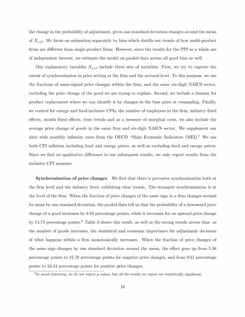
Our explanatory variables Xi,j,t include three sets of variables: First, we try to capture the

extent of synchronization in price setting at the firm and the sectoral level. To this purpose, we use

the fractions of same-signed price changes within the firm, and the same six-digit NAICS sector,

excluding the price change of the good we are trying to explain. Second, we include a dummy for

product replacement where we can identify it by changes in the base price at resampling. Finally,

we control for energy and food-inclusive CPIs, the number of employees in the firm, industry fixed

effects, month fixed effects, time trends and as a measure of marginal costs, we also include the

average price change of goods in the same firm and six-digit NAICS sector. We supplement our

data with monthly inflation rates from the OECD “Main Economic Indicators (MEI).” We use

both CPI inflation including food and energy prices, as well as excluding food and energy prices.

Since we find no qualitative difference in our subsequent results, we only report results from the

inclusive CPI measure.

Synchronization of price changes We find that there is pervasive synchronization both at

the firm level and the industry level, exhibiting clear trends. The strongest synchronization is at

the level of the firm: When the fraction of price changes of the same sign in a firm changes around

its mean by one standard deviation, the pooled data tell us that the probability of a downward price

change of a good increases by 8.82 percentage points, while it increases for an upward price change

by 14.73 percentage points.6 Table 3 shows this result, as well as the strong trends across bins: as

the number of goods increases, the statistical and economic importance for adjustment decisions

of what happens within a firm monotonically increases. When the fraction of price changes of

the same sign changes by one standard deviation around the mean, the effect goes up from 5.38

percentage points to 15.78 percentage points for negative price changes, and from 9.61 percentage

points to 24.24 percentage points for positive price changes.

6To avoid cluttering, we do not report p-values, but all the results we report are statistically significant.

16

These large complementarities in adjustment decisions within firms plus the strong trends un-

derline our message that multi-product firms price differently than a collection of single-product

firms. The trends also suggest that the importance of firm-specific shocks becomes more important

as the number of goods increases. This is related to work by Boivin et al. (2009). Comparing the

explanatory power from a regression with and without firm-specific variables also emphasizes their

importance: when we omit the firm-specific fraction and the average price change of goods from

an otherwise unchanged regression, R2 goes down from 48% to 30%. Curiously, the R2 also shows

a positive trend with the number of goods.

The importance of the multi-product dimension for pricing is further reinforced when we con-

sider synchronization with decisions in the industry: There, we find that synchronization is much

weaker, especially as the number of goods increases. On average, the probability of a downward

price change of a good increases by 1.32 percentage points, while the probability of an upward

price change of a good increases by 2.27 percentage points when the industry-level fraction of price

changes of the same sign moves around the mean by one standard deviation. As the number of

goods increases, the effect goes down from 3.07 percentage points to 0.21 percentage points for

positive price changes, and from 2.10 percentage points to −1.51 percentage points for negative

price changes.

Here, it is important to emphasize that our synchronization results are not due to a purely

“statistical” effect. One could think that the variance of the fraction of price changes of the same

sign in a firm decreases as the number of goods increases. This could imply a larger estimated

synchronization coefficient. However, there is no such trend in the data for the variance of fractions.

In fact, the opposite holds true.

State-dependent response to inflation It is a long-debated and important question in

monetary economics whether price setting is time-dependent or state-dependent. We contribute

some evidence by explicitly considering the role played by inflation, an important aggregate shock,

for pricing decisions. We find what one would expect from a model where firms adjust prices in

a state-dependent fashion. As Table 3 shows, the likelihood of a price decrease decreases with

higher CPI inflation while the likelihood of a price increase increases. When CPI inflation changes

17

by one standard deviation around the mean, the probability of a negative price change of a good

decreases by 0.21 percentage points, while the probability of a positive price change increases by

0.17 percentage points. The effects are both statistically and economically significant.

Robustness We conduct a battery of robustness tests for these good-level regressions. First,

we consider different levels of aggregation for our definition of the industry variable. In conducting

this extension, in addition to checking for robustness, we are motivated by the theoretical results

in Bhaskar (2002) that synchronization is likely to be higher within groups with higher elasticity of

substitution among goods, that is, at a more disaggregated industry level. Table A.8 in Appendix

A presents results using an industry classification at the 2-digit NAICS level. It shows that at this

higher level of aggregation, prices in the pooled data specification are much less synchronized at the

industry level, compared to Table 3. Table A.8 also shows results for the four good bins separately.

The general result of higher firm level synchronization and lower industry level synchronization as

we move to higher good bins is robust to this alternate definition of industry.7 Compared to Table

3 and as predicted by Bhaskar (2002), however, we see the significant extent to which the industry

level synchronization has decreased across all bins.

Second, we check that clustering standard errors at the industry level do not affect out findings.

Third, we use a polynomial function for the size of firms to control for non-linear size effects in the

regressions. Our results do not change due to this modification. Fourth, we use a CPI measure

that excludes food and energy prices. Finally, we estimate the multinomial logit model only for the

adjustment decisions for the largest sales-value item of each firm. Again, our results do not change

due to this modification, in particular, with respect to synchronization.8

7This result is similar to that of Cornille and Dossche (2008) and Dhyne and Konieczny (2007) who use the BelgianPPI and the CPI respectively. They use the Fisher-Konieczny measure of synchronization and find that prices tendto be more synchronized at a more disaggregated industry level. Neither of these papers look at the level of the firm,however, which is the focus of our paper, and also the factor that quantitatively matters most in our data.

8The results mentioned in the second robustness paragraph are available upon request from the authors.

18

4 Theory

Compared to the existing literature, our main theoretical challenge is to explain the various trends

we observe in price setting as we vary the number of goods per firm, an analysis that has not been

undertaken before. We do so by developing a model of pricing by state-dependent multi-product

firms. We find that varying only one parameter – the firm-specific menu cost of price adjustment –

allows us to match the trends in the data. Since the mapping from the good bins that we construct

in the empirical section to the number of goods in the model is not direct, we view our exercise in

this section as qualitative in nature. Nonetheless, the results from simulations of our model allow

us to validate modeling features that are needed to explain the empirical trends.

4.1 Model

We use a partial equilibrium setting of a firm that decides each period whether to update the

prices of its n goods indexed by i ∈ (1, 2, 3), and what prices to charge if it updates. Our model

is similar to the ones in Sheshinski and Weiss (1992), Midrigan (2011), and Alvarez and Lippi

(2013). The main difference is that compared to Sheshinski and Weiss (1992) and Alvarez and

Lippi (2013) we allow for a stochastic aggregate shock and correlated idiosyncratic shocks across

goods produced by a firm, while compared to Midrigan (2011), we solve for equilibrium as we vary

n. In particular, the latter variation allows us to make two important contributions. First, we can

solve for trends in price-setting behavior with respect to how many goods firms produce. Second,

we can compute trends in synchronization of price-setting by comparing 2-good and 3-good firms.

Since no measures of synchronization can be computed in the one-good case, the comparison of

2-good and 3-good firms is necessary to model trends in synchronization of adjustment decisions.

This focus on synchronization also additionally distinguishes our model from the aforementioned

papers.

Production technology and demand

In our model, the firm produces output ci,t of good i using a technology that is linear in labor

li,t:

ci,t = Ai,t li,t

19

where Ai,t is a good-specific productivity shock that follows an exogenous process:

lnAi,t = ρiA lnAi,t−1 + εiA,t

where E[εiA,t] = 0 and cov(Ai,t, Aj,t) = σ2A for i = j and σ2Ai,Ajfor i 6= j. That is, as in Midrigan

(2011) we allow the productivity shock across goods produced by the same firm to be correlated.

The firm’s product i is subject to the following demand:

ci,t =

(pi,tPt

)−θCt i = 1, 2, ..., n

where Ct is aggregate consumption, Pt is the aggregate price level, pi,t is the price of good i, and

θ is the elasticity of substitution across goods. In this partial equilibrium setting, we normalize

Ct = C. We also assume that the price level Pt exogenously follows a random walk with a drift:

lnPt = µP + lnPt−1 + εP,t

where E[εP,t] = 0 and var(εP,t) = (σP )2. Given our assumption about technology, the real marginal

cost of the firm for good i, MCi,t, is therefore given by: MCi,t = WtAi,tPt

, where Wt is the nominal

wage. We normalize WtPt

= w.

Given this setup, the firm maximizes the expected discounted sum of profits from selling all of

its goods. Total period gross profits are given by:

πt =n∑i

(pi,tPt− w

Ai,t

)(pi,tPt

)−θC.

The problem of the firm is to choose whether to update all prices in a given period, and if so, by

how much. Whenever it updates prices, it has to pay a menu cost K, which we discuss next.

Menu cost technology

In particular, this “menu cost” comes in the form of a constant, firm-specific cost K(n) > 0 for

adjusting one, or more than one, of its prices. This assumption of firm-specificity directly implies

that the firm will either adjust all its prices at the same time or adjust none at all. In our dataset,

20

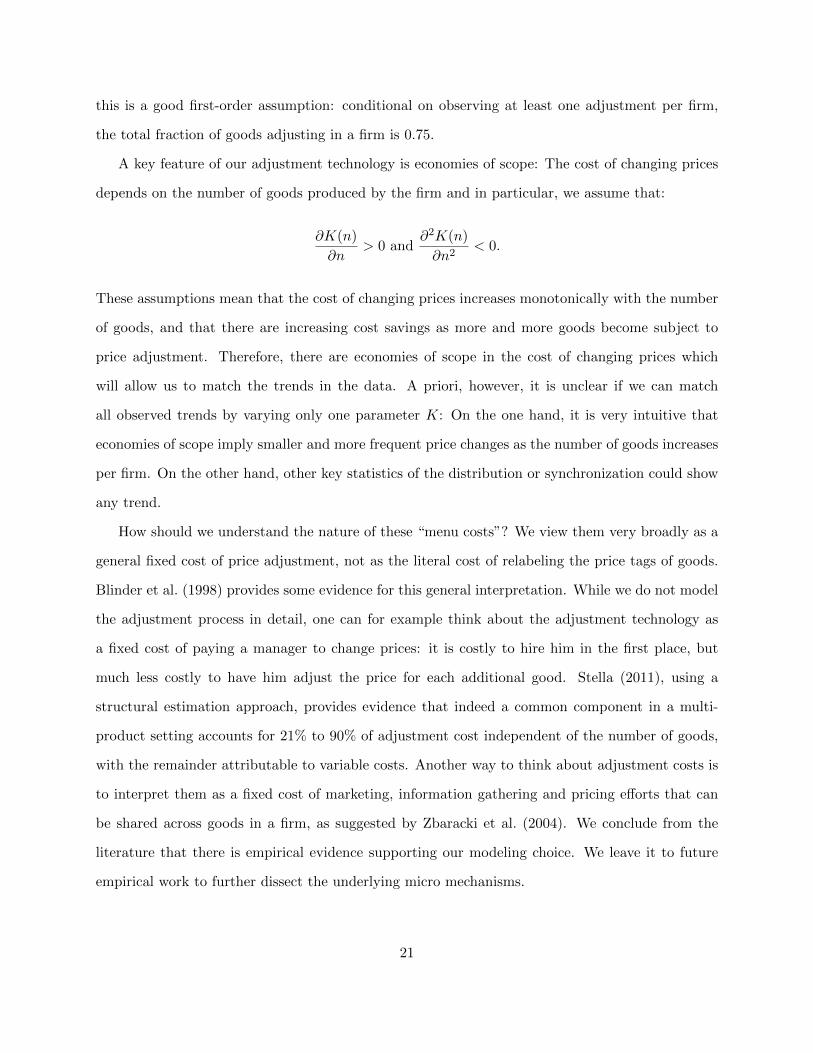
this is a good first-order assumption: conditional on observing at least one adjustment per firm,

the total fraction of goods adjusting in a firm is 0.75.

A key feature of our adjustment technology is economies of scope: The cost of changing prices

depends on the number of goods produced by the firm and in particular, we assume that:

∂K(n)

∂n> 0 and

∂2K(n)

∂n2< 0.

These assumptions mean that the cost of changing prices increases monotonically with the number

of goods, and that there are increasing cost savings as more and more goods become subject to

price adjustment. Therefore, there are economies of scope in the cost of changing prices which

will allow us to match the trends in the data. A priori, however, it is unclear if we can match

all observed trends by varying only one parameter K: On the one hand, it is very intuitive that

economies of scope imply smaller and more frequent price changes as the number of goods increases

per firm. On the other hand, other key statistics of the distribution or synchronization could show

any trend.

How should we understand the nature of these “menu costs”? We view them very broadly as a

general fixed cost of price adjustment, not as the literal cost of relabeling the price tags of goods.

Blinder et al. (1998) provides some evidence for this general interpretation. While we do not model

the adjustment process in detail, one can for example think about the adjustment technology as

a fixed cost of paying a manager to change prices: it is costly to hire him in the first place, but

much less costly to have him adjust the price for each additional good. Stella (2011), using a

structural estimation approach, provides evidence that indeed a common component in a multi-

product setting accounts for 21% to 90% of adjustment cost independent of the number of goods,

with the remainder attributable to variable costs. Another way to think about adjustment costs is

to interpret them as a fixed cost of marketing, information gathering and pricing efforts that can

be shared across goods in a firm, as suggested by Zbaracki et al. (2004). We conclude from the

literature that there is empirical evidence supporting our modeling choice. We leave it to future

empirical work to further dissect the underlying micro mechanisms.

21

4.2 Results

4.2.1 Computation

We solve the given problem for a firm that produces n = 1, 2, and 3 goods. First, we employ

collocation methods to find the policy functions of the firm. Second, given the policy functions, we

simulate time series of shocks and corresponding adjustment decisions for many periods. Finally,

we compute statistics of interest for each simulation and good, and across simulations. We also

estimate a multi-nomial logit model of adjustment decisions using the simulated data to compare

our theoretical results with the empirical findings. Appendix B provides further details about

computation and analysis.

We mostly follow the literature in our choice of parameters. Since our model is monthly, we

choose a discount rate β of (0.96)112 . We choose θ to be 4, which implies a markup of 33%. To

parametrize the aggregate exogenous processes, we set the trend in aggregate inflation µP to be

a monthly increase of 0.21% and the standard deviation σP to be 0.32%. These values are taken

from Nakamura and Steinsson (2008). To parametrize the idiosyncratic productivity shock, we

use the NBER productivity database covering 459 sectors from 1984 − 1996 and compute for our

productivity process an estimate of ρ = 0.96 for the AR(1) parameter and σA = 2% for the

standard deviation.9 For the firms with 2 and 3 goods, we use the same values for the persistence

and variance of the all idiosyncratic productivity shocks, but following Midrigan (2011), we allow

for a correlation of 0.65 among the good-specific productivity shocks. Finally, we use a value of

K such that menu costs are a 0.40% of steady-state revenues for the 1-good firm, 0.70% for a 2-good

firm, and 0.80% for a 3-good firm. These choices for K allow us to replicate, as shown below, the

trends across the good bins that we document empirically.

4.2.2 Findings

We find that the model predicts clear and systematic trends in the key price-setting statistics as we

increase the number of goods from 1 to 3. The trends align, qualitatively, with our empirical finding

9A persistent productivity process is a common specification in the literature. For example, Midrigan (2011) usesa random walk process for idiosyncratic productivity shocks.

22

that multi-product firms behave systematically different from a collection of multiple single-product

firms. We present the main results from our simulations in Table 4.

First, we find that the frequency of price changes goes up from 13.89% to 20.21% while the mean

absolute size of price changes goes down from 5.42% to 4.18% as we increase the number of goods.

Second, the decrease in the absolute size of price changes also holds for both positive and negative

prices changes: they go down from 5.53% to 4.34% and from −5.24% to −3.95% respectively. Third,

the fraction of small price changes increases from 2.29%, barely none, to 19.54%. Thus, while firms

with more goods change prices more frequently, they do so by smaller amounts on average. Fourth,

we also see that the fraction of positive price changes decreases from 62.63% to 60.31%. Thus, as

in the data, firms with more goods adjust downwards more frequently. Finally, the model predicts

that kurtosis increases from 1.45 to 2.03, again consistent with our empirical findings.

What is the mechanism behind our results? For simplicity, compare a 1-good firm with a 2-good

firm. For the case of a 2-good firm, when the firm decides to pay the firm-specific menu cost to

adjust one of the prices, it also gets to change the price of the other good for free. This leads to

a higher average frequency of price changes. At the same time, for the 2-good firm, since a lot of

price changes happen even when the desired price is not very different from the current price of

the good, the mean absolute size of price changes is lower. This smaller mean also implies that the

fraction of “small” price changes is higher for the 2-good firm. In fact, for the 1-good firm, which

is the standard menu cost model, the fraction of small price changes is negligible because in that

case, the firm adjusts prices only when the desired price is very different from the current price.

What causes the decrease in the fraction of positive price changes? With trend inflation, firms

adjust downwards only when they receive very big negative productivity shocks. With firm-specific

menu costs, since the firm adjusts both prices when the desired price of one good is very far from

its current price, it is now more sustainable to have a higher fraction of downward price changes.

Finally, kurtosis increases as we go from one good to two goods because of a higher fraction of price

changes in the middle of the distribution.

Next, we address trends in synchronization of individual good-level price changes. Using sim-

ulated data, we run the same multinominal logit regression as in the empirical section given by

23

specification (3). Our explanatory variables now include the fraction of same-signed adjustment

decisions at time t within the firm and Πt is the inflation rate at time t. It is important to emphasize

here the need to go beyond the 2-good case in Midrigan (2011) or Sheshinski and Weiss (1992), and

consider a 3-good case. Otherwise, we cannot check if the model predicts trends in synchronization

of price changes that are consistent with the empirical findings.

We find from our simulations that the strength of synchronization, that is the coefficient estimate

in the logit regressions for the fraction of other goods of the firm changing in the same direction,

increases as we go from a 2-good firm to a 3-good firm. Table 4 shows this. This effect is first simply

due to the underlying economies of scope: they increase the probability of simultaneous adjustment

decisions in a firm as the number of goods increases. Second, correlated shocks in our model also

play a role for synchronization since, as is intuitive with correlated shocks across goods, desired

prices of goods within the firm become more likely to move in the same direction. Importantly, as

is the case empirically, this is also the case with both upwards and downwards price changes.

In addition, our simulation results make clear that the simulations predict that positive price

adjustment decisions are more synchronized than negative adjustment decisions since the synchro-

nization coefficient for upwards price adjustment decisions is always higher than the coefficient for

downwards adjustment decisions. This difference in synchronization probabilities is due to positive

trend inflation. If we omit positive trend inflation from the model, the difference disappears. The

model thus matches our findings on synchronization established in the empirical section.

4.2.3 Robustness

In this section, we discuss alternative modeling mechanisms to economies of scope in menu costs.

Our main finding is that each alternative mechanism can match some of the trends, but it usually

also fails in matching some other trends. This validates the choice of our main, parsimonious model

while suggesting which other mechanisms may be important depending on other modeling interests.

All detailed results, if not in Appendix B, are available on request.

First, we investigate whether correlated shocks are the most important feature of the model as

opposed to economies of scope in menu costs. When we shut down correlation of productivity shocks

24

by setting σAi,Aj = 0, in fact we can still match qualitatively all of our trends in pricing statistics.10

We summarize this experiment in Table B.1 in Appendix B. Moreover, we have also simulated a

model with correlation of the productivity shocks but without complementarities in menu costs.

Table B.2 summarizes this modification, showing that correlation alone cannot generate the trends

found in the data. Thus, economies of scope in menu costs are critical to generate the trends in

the model. In particular, just firm-specific menu costs, without economies of scope and absent

correlation, are not enough to replicate the trends from our empirical section. Table B.3 shows the

results from a model specification where menu costs are firm-specific, but the per-good menu cost

is the same across firms with 1, 2, or 3 goods.

Second, we investigate the possibility that perhaps our results are driven by the fact that firms

that produce more goods also produce more substitutable goods. We simulate a specification of 2-

good and 3-good firms with no economies of scope in the cost of adjusting prices and no correlation

of productivity shocks but with an elasticity of substitution among goods that is higher than that

of the 1 good firm. While matching the trends in frequency, size, and fraction of positive price

changes, we generally find that this specification fails to match trends in the fraction of small price

changes, kurtosis, and synchronization as we increase the number of goods.

Third, there might be concern that our synchronization results could be due to purely mechan-

ical, statistical reasons. To investigate this possibility, we perform two tests. In the first, we run a

Monte-Carlo exercise based on a simple statistical model of price changes. We model price changes

as i.i.d. Bernoulli trials with a fixed probability of success. Using simulated time series for an ar-

bitrary number of goods, we estimate our synchronization equation. We find no mechanical trend

in synchronization. In the second test, we use the single-good firm from our simulation exercise

and model a multi-product firm as a collection of multiple, independent single-product firms. That

is, a 2-good firm now is simply a collection of two single-good firms, with no economies of scope

in cost of adjusting prices and no correlated shocks. Similarly, a 3-good firm is a collection of

three independent single-good firms. When we run our synchronization test with simulated data

from these specifications, we find that the model cannot produce synchronization results that are

10It is still worthwhile to include this feature in the baseline model since it is intuitive, has been used frequently inthe literature, and does generate higher synchronization of price changes.

25

consistent with the empirical findings. For example, the synchronization coefficients estimated us-

ing simulated data become smaller as we move from two single-good to three single-good firms.

Incidentally, this specification of multiproduct firms as multiple single-good firms fails to match

any of our aggregate trends in price-setting, such as the frequency of price changes. We summarize

results in Table B.4 in Appendix B. These results highlight the need to model a multi-product firm

as distinctly different from an aggregate of multiple single-product firms.

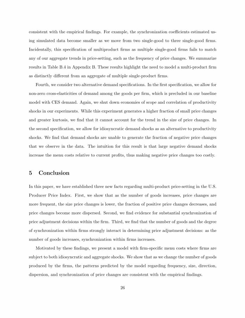
Fourth, we consider two alternative demand specifications. In the first specification, we allow for

non-zero cross-elasticities of demand among the goods per firm, which is precluded in our baseline

model with CES demand. Again, we shut down economies of scope and correlation of productivity

shocks in our experiments. While this experiment generates a higher fraction of small price changes

and greater kurtosis, we find that it cannot account for the trend in the size of price changes. In

the second specification, we allow for idiosyncratic demand shocks as an alternative to productivity

shocks. We find that demand shocks are unable to generate the fraction of negative price changes

that we observe in the data. The intuition for this result is that large negative demand shocks

increase the menu costs relative to current profits, thus making negative price changes too costly.

5 Conclusion

In this paper, we have established three new facts regarding multi-product price-setting in the U.S.

Producer Price Index. First, we show that as the number of goods increases, price changes are

more frequent, the size price changes is lower, the fraction of positive price changes decreases, and

price changes become more dispersed. Second, we find evidence for substantial synchronization of

price adjustment decisions within the firm. Third, we find that the number of goods and the degree

of synchronization within firms strongly interact in determining price adjustment decisions: as the

number of goods increases, synchronization within firms increases.

Motivated by these findings, we present a model with firm-specific menu costs where firms are

subject to both idiosyncratic and aggregate shocks. We show that as we change the number of goods

produced by the firms, the patterns predicted by the model regarding frequency, size, direction,

dispersion, and synchronization of price changes are consistent with the empirical findings.

26

References

Alvarez, F. and F. Lippi (2013): “Price Setting with Menu Cost for Multi-Product Firms,”Forthcoming, Econometrica.

Bernard, A., S. Redding, and P. Schott (2010): “Multi-Product Firms and Product Switch-ing,” American Economic Review, 100, 70–97.

Bhaskar, V. (2002): “On Endogenously Staggered Prices,” Review of Economic Studies, 69,97–116.

Blinder, A. S., E. R. D. Canetti, D. E. Lebow, and J. B. Rudd (1998): Asking AboutPrices: A New Approach to Understanding Price Stickiness, Russell Sage Foundation, New York,N.Y.

Boivin, J., M. P. Giannoni, and I. Mihov (2009): “Sticky Prices and Monetary Policy: Evi-dence from Disaggregated US Data,” American Economic Review, 99, 350–84.

Carvalho, C. (2006): “Heterogeneity in Price Stickiness and the Real Effects of MonetaryShocks,” The BE Journal of Macroeconomics (Frontiers), 2.

Cornille, D. and M. Dossche (2008): “Some Evidence on the Adjustment of Producer Prices,”Scandinavian Journal of Economics, 110, 489–518.

Dhyne, E. and J. Konieczny (2007): “Temporal Distribution of Price Changes : Staggeringin the Large and Synchronization in the Small,” Research series 200706-02, National Bank ofBelgium.

Eichenbaum, M. S., N. Jaimovich, S. Rebelo, and J. Smith (2013): “How Frequent AreSmall Price Changes?” Forthcoming, American Economic Journal: Macroeconomics.

Fisher, T. C. G. and J. D. Konieczny (2000): “Synchronization of Price Changes by Multi-product Firms: Evidence from Canadian Newspaper Prices,” Economics Letters, 68, 271–277.

Gagnon, E. (2009): “Price Setting During Low and High Inflation: Evidence from Mexico,” TheQuarterly Journal of Economics, 124, 1221–1263.

Goldberg, P. and R. Hellerstein (2009): “How Rigid Are Producer Prices?” Federal ReserveBank of New York Staff Reports.

Goldberg, P., A. Khandelwal, N. Pavcnik, and P. Topalova (2008): “Multi-Product Firmsand Product Turnover in the Developing World: Evidence from India,” Review of Economics andStatistics forthcoming.

Golosov, M. and R. E. Lucas Jr. (2007): “Menu Costs and Phillips Curves,” Journal ofPolitical Economy, 115, 171–199.

Gopinath, G. and O. Itskhoki (2010): “Frequency of Price Adjustment and Pass-Through,”The Quarterly Journal of Economics, 125, 675–727.

Gopinath, G., O. Itskhoki, and R. Rigobon (2010): “Currency Choice and Exchange RatePass-Through,” American Economic Review, 100, 304–36.

27

Klenow, P. J. and O. Kryvtsov (2008): “State-Dependent or Time-Dependent Pricing: DoesIt Matter for Recent U.S. Inflation?” The Quarterly Journal of Economics, 123, 863–904.

Klenow, P. J. and B. A. Malin (2010): “Microeconomic Evidence on Price-Setting,” inHandbook of Monetary Economics, ed. by B. M. Friedman and M. Woodford, Elsevier, vol. 3 ofHandbook of Monetary Economics, chap. 6, 231–284.

Lach, S. and D. Tsiddon (1996): “Staggering and Synchronization in Price-Setting: Evidencefrom Multiproduct Firms,” American Economic Review, 86, 1175–96.

——— (2007): “Small Price Changes and Menu Costs,” Managerial and Decision Economics, 28,649–656.

Midrigan, V. (2011): “Menu Costs, Multi-Product Firms, and Aggregate Fluctuations,”Econometrica, 79.

Miranda, M. J. and P. L. Fackler (2002): Applied Computational Economics and Finance,MIT Press.

Nakamura, E. and J. Steinsson (2008): “Five Facts about Prices: A Reevaluation of MenuCost Models,” Quarterly Journal of Economics, 123, 1415–1464.

Neiman, B. (2011): “A State-Dependent Model of Intermediate Goods Pricing,” Journal ofInternational Economics, 85, 1–13.

Sheshinski, E. and Y. Weiss (1992): “Staggered and Synchronized Price Policies under Inflation:The Multiproduct Monopoly Case,” Review of Economic Studies, 59, 331–59.

Stella, A. (2011): “The Magnitude of Menu Costs: A Structural Estimation,” Working paper,Federal Reserve Board.

Zbaracki, M. J., M. Ritson, D. Levy, S. Dutta, and M. Bergen (2004): “Managerial andCustomer Costs of Price Adjustment: Direct Evidence from Industrial Markets,” The Review ofEconomics and Statistics, 86, 514–533.

28

6 Tables

Table 1: Summary Statistics by Number of Goods

Number of Goods1-3 3-5 5-7 >7

Mean Employment 2996 1427 1132 1016Median Employment 427 155 195 296

% of Prices 17.15 43.53 18.16 21.16

Mean # of Goods 2.21 4.05 6.06 10.26Std. Error # Goods 0.01 0.00 0.01 0.11Std. Dev. # Goods 0.77 0.34 0.40 4.88Minimum # of Goods 1 3.01 5.01 7.02Maximum # of Goods 3 5 7 7725% Percentile # Goods 1.78 3.94 5.91 7.98Median # Goods 2 4 6 875% Percentile # Goods 3 4 6 11.77

Number of Firms 9111 13577 3532 2160

We compute statistics from the PPI data according the number ofgoods. We calculate mean and median employment by taking meansand medians of the number of employees per good across firms in abin/overall category. % of Prices denotes the fraction of prices in thePPI set by firms in each bin.

Table 2: Coefficient of Variation of Price Changes

Number of Goods1-3 3-5 5-7 >7

Firm-Based 1.02 1.15 1.30 1.55(0.01) (0.01) (0.02) (0.02)

Good-Based 0.96 1.00 1.10 1.24(0.01) (0.01) (0.02) (0.02)

For the first column, we compute the coefficient of vari-ation at the level of the firm pooling all price changes.Then, we take medians across firms, bin by bin. For thesecond column, we compute the coefficient of variation foreach good, take the median across goods within the firmand then medians across firms.

29

Table 3: Marginal Effects by Number of Goods, ± 1/2 Std. Dev.

1-3 Goods 3-5 Goods 5-7 Goods >7 Goods All Goods All Goods†Negative Change

Fraction Industry 2.10% 1.41% 0.89% -1.51% 1.32% 6%Fraction Firm 5.38% 6.52% 9.92% 15.78% 8.82% -πCPI -0.08% -0.14% -0.17% -0.54% -0.21% -0.25%

Positive Change

Fraction Industry 3.07% 2.12% 1.55% 0.21% 2.27% 10.29%Fraction Firm 9.61% 11.46% 15.94% 24.24% 14.74% -πCPI 0.17% 0.10% 0.14% 0.35% 0.17% 0.16%

R2 42.85% 47.93% 48.33% 49.10% 47.56% 29.33%

The table shows the bin-specific marginal effects in percentage points of a one-standard deviation change in theexplanators around the mean on the probability of adjusting prices upwards or downwards. Marginal effects arecalculated for a model estimated for each bin separately as well as on the pooled data. All reported effects arestatistically significantly different from zero. †Results from omitting firm-specific variables are shown in the lastcolumn.

Table 4: Results of Simulation

1 Good 2 Goods 3 Goods

Frequency of price changes 13.89% 17.85% 20.21%Size of absolute price changes 5.42% 4.60% 4.18%Size of positive price changes 5.53% 4.66% 4.34%Size of negative price changes -5.26% -4.52% -3.95%Fraction of positive price changes 62.92% 62.03% 60.31%Fraction of small price changes 2.41% 15.92% 19.54%Kurtosis 1.45 1.72 2.031st Percentile -7.24% -7.94% -8.68%99th Percentile 7.45% 8.36% 9.04%

Synchronization measures:Fraction, Upwards Adjustments - 31.29 38.65Fraction, Downwards Adjustments - 30.72 37.72

Correlation coefficient - 0.65 0.65Menu Cost 0.40% 0.70% 0.80%

We perform stochastic simulation of our model in the 1-good, 2-good and 3-goodcases and record price adjustment decisions in each case, allowing for correlation ofthe productivity shocks Ai,t in the multi-good cases. Then, we calculate statisticsfor each case as described in the text. In the 2-good and the 3-good cases, we reportthe mean of the good-specific statistics. We obtain the synchronization measurefrom a multinomial logit regression analogous to the empirical multinomial logitregression. We control for inflation. Menu costs are given as a percentage of steadystate revenues.

30

7 Graphs

Figure 1: Mean Frequency of Price Changes with 95% Bands

15%

17%

19%

21%

23%

25%

27%

29%

31%

1-3 3-5 5-7 >7

Fre

qu

ency

of

pri

ce c

han

ges

Number of goods

Mean Frequency of Price Changes with 95% Bands

Based on the PPI data we group firms by the number of goods. We compute the mean frequency of price changes

in these groups in the following way. First, we compute the frequency of price change at the good level. Then,

we compute the median frequency of price changes across goods at the firm level. Finally, we report the mean

across firms in a given group. We compute upper and lower bounds of the error bands as ± 1.96 * std. error

across firms.

31

Figure 2: Median Frequency of Price Changes

10%

12%

14%

16%

18%

20%

22%

24%

1-3 3-5 5-7 >7

Med

ian

fre

qu

ency

of

pri

ce c

han

ges

Number of goods

Median Frequency of Price Changes

Based on the PPI data we group firms by the number of goods. We compute the median frequency of price

changes in these groups in the following way. First, we compute the frequency of price change at the good level.

Then, we compute the median frequency of price changes across goods at the firm level. Finally, we report the

median across firms in a given group.

32

Figure 3: Mean Fraction of Positive Price Changes with 95% Bands

61%

61%

62%

62%

63%

63%

64%

64%

65%

65%

66%

1-3 3-5 5-7 >7

Frac

tion

of p

ositi

ve p

rice

cha

nges

Number of Goods

Mean Frequency of Positive Price Changes with 95% Bands

Based on the PPI data we group firms by the number of goods. We compute the mean fraction of positive price

changes in these groups in the following way. First, we compute the number of strictly positive good level price

changes over all zero and non-zero price changes for a given firm. Then, we report the mean across firms in a

given group. We compute upper and lower bounds of the error bands as ± 1.96 * std. error across firms.

33

Figure 4: Mean Absolute Size of Price Changes with 95% Bands

6.00%

6.50%

7.00%

7.50%

8.00%

8.50%

9.00%

1-3 3-5 5-7 >7

Ab

solu

te s

ize

of

pri

ce c

han

ges

Number of goods

Mean Absolute Size of Price Changes with 95% Bands

Based on the PPI data we group firms by the number of goods. We compute the mean absolute size of price

changes in these groups in the following way. First, we compute the percentage change to last observed price

at the good level. Then, we compute the median size of price changes across goods at the firm level. Then, we

report the mean across firms in a given group. We compute upper and lower bounds of the error bands as ± 1.96

* std. error across firms.

34

Figure 5: Mean Size of Positive and Negative Price Changes with 95% Bands

Based on the PPI data we group firms by the number of goods. We compute the mean size of positive price

changes in these groups in the following way. First, we compute the percentage change to last observed price

at the good level. Then, we compute the median size of price changes across goods at the firm level. Then, we

report the mean across firms in a given group. We compute upper and lower bounds of the error bands as ± 1.96

* std. error across firms. 35

Figure 6: Mean Fraction of Small Price Changes with 95% Bands

30%

35%

40%

45%

50%

55%

60%

1-3 3-5 5-7 >7

Fra

ctio

n o

f sm

all

pri

ce c

han

ges

Number of goods

Mean Fraction of Small Price Changes with 95% Bands

Based on the PPI data we group firms by the number of goods. We compute the mean fraction of small price

changes in these groups in the following way. First, we compute the fraction of price changes that are smaller

than 0.5 times the mean absolute percentage size of price changes across all goods in a firm. Then, we report

the mean across firms in a given group. We compute upper and lower bounds of the error bands as ± 1.96 * std.

error across firms.

36

Figure 7: Mean Kurtosis of Price Changes with 95% Bands

4

6

8

10

12

14

16

18

20

1-3 3-5 5-7 >7

Ku

rto

sis

of

pri

ce c

han

ges

Number of goods

Mean Kurtosis of Price Changes with 95% Bands

Based on the PPI data we group firms by the number of goods. We compute the mean kurtosis of price changes

in these groups in the following way. First, we compute the kurtosis of price changes at the firm level, defined as

the ratio of the fourth moment about the mean and the variance squared of percentage price changes. Then, we

report the mean across firms in a given group. We compute upper and lower bounds of the error bands as ± 1.96

* std. error across firms.

37

Figure 8: Mean First and 99th Percentile of Price Changes with 95% Bands

Based on the PPI data we group firms by the number of goods. We compute the mean size of positive price

changes in these groups in the following way. First, we compute the percentage change to last observed price

at the good level. Then, we compute the median size of price changes across goods at the firm level. Then, we

report the mean across firms in a given group. We compute upper and lower bounds of the error bands as ± 1.96

* std. error across firms.

38

APPENDIX A

This appendix contains empirical robustness results to which we make reference in the text.

Table A.1: Distribution of Firms across Sectors and Bins

Sector Bin 1 Bin 2 Bin 3 Bin 4 Total

11 58.1% 30.95% 5.24% 5.71% 100%1.36% 0.5% 0.32% 0.58% 0.77%

21 74.48% 19.84% 3.6% 2.09% 100%7.17% 1.32% 0.91% 0.87% 3.15%

22 19.11% 9.95% 10.73% 60.21% 100%0.82% 0.29% 1.21% 11.16% 1.4%

23 48.25% 51.75% 0% 0% 100%3.08% 2.29% 0% 0% 2.09%

31 28.01% 49.92% 15.05% 7.02% 100%12% 14.79% 16.96% 13.05% 14.02%

32 34.17% 47.73% 13.33% 4.77% 100%18.82% 18.17% 19.31% 11.4% 18.01%

33 28.72% 52.85% 13.32% 5.11% 100%28.76% 36.59% 35.1% 22.22% 32.76%

42 27.23% 61.95% 7.33% 3.49% 100%1.74% 2.74% 1.23% 0.97% 2.09%

44 35.28% 47.18% 7.93% 9.6% 100%3.78% 3.49% 2.23% 4.46% 3.5%

45 28.12% 50.94% 7.5% 13.44% 100%1.01% 1.26% 0.71% 2.09% 1.17%

48 36.74% 48.17% 6.55% 8.54% 100%2.69% 2.44% 1.26% 2.72% 2.4%

49 45.03% 38.6% 8.19% 8.19% 100%0.86% 0.51% 0.41% 0.68% 0.63%

51 30.79% 48.31% 8.85% 12.05% 100%3.65% 3.96% 2.76% 6.21% 3.88%

52 28.07% 31.65% 20.45% 19.83% 100%4.03% 3.14% 7.73% 12.37% 4.7%

53 59.56% 33.81% 2.37% 4.27% 100%4.21% 1.65% 0.44% 1.31% 2.31%

54 37.34% 53.32% 8.51% 0.83% 100%2.01% 1.99% 1.21% 0.19% 1.76%

56 29.81% 35.82% 29.09% 5.29% 100%1.39% 1.15% 3.56% 1.07% 1.52%

62 21.06% 38.89% 17.44% 22.61% 100%1.82% 2.33% 3.97% 8.49% 2.83%

71 26.87% 62.69% 10.45% 0% 100%

Continued on next page

1

Table A.1 – continued from previous pageSector Bin 1 Bin 2 Bin 3 Bin 4 Total

0.2% 0.32% 0.21% 0% 0.24%72 25% 65.87% 7.69% 1.44% 100%

0.58% 1.06% 0.47% 0.15% 0.76%

Total 32.71% 47.32% 12.44% 7.53% 100%100% 100% 100% 100% 100%

The table shows the percentage of firms in the PPI that belong to a bin in a giventwo-digit NAICS category (each first line per industry) and the percentage in anindustry given a bin (each second line). Bin 1 groups firms with 1 to 3 goods, bin 2firms with 3 to 5 goods, bin 3 firms with 5 to 7 goods and bin 4 firms with more than7 goods

Table A.2: Distribution of Firms across Sectors and Bins

Sector Bin 1 Bin 2 Bin 3 Bin 4 Total

111 72.73% 19.32% 3.41% 4.55% 100%0.72% 0.13% 0.09% 0.19% 0.32%

112 30% 35% 15% 20% 100%0.07% 0.05% 0.09% 0.19% 0.07%

113 50% 45.45% 4.55% 0% 100%0.49% 0.31% 0.12% 0% 0.32%

114 57.14% 7.14% 7.14% 28.57% 100%0.09% 0.01% 0.03% 0.19% 0.05%

211 25.3% 45.78% 15.66% 13.25% 100%0.23% 0.29% 0.38% 0.53% 0.3%

212 81.33% 15.59% 2.16% 0.93% 100%5.89% 0.78% 0.41% 0.29% 2.37%

213 71.76% 24.43% 3.05% 0.76% 100%1.05% 0.25% 0.12% 0.05% 0.48%

221 19.11% 9.95% 10.73% 60.21% 100%0.82% 0.29% 1.21% 11.16% 1.4%

236 48.25% 51.75% 0% 0% 100%3.08% 2.29% 0% 0% 2.09%

311 24.47% 46.58% 18.93% 10.02% 100%5.43% 7.15% 11.05% 9.66% 7.26%

312 31.62% 38.14% 21.65% 8.59% 100%1.03% 0.86% 1.85% 1.21% 1.06%

313 27.15% 62.37% 8.06% 2.42% 100%1.13% 1.79% 0.88% 0.44% 1.36%

314 25.53% 65.77% 5.71% 3% 100%0.95% 1.69% 0.56% 0.49% 1.22%

Continued on next page

2

Table A.2 – continued from previous pageSector Bin 1 Bin 2 Bin 3 Bin 4 Total

315 34.63% 52.03% 9.92% 3.41% 100%2.38% 2.47% 1.79% 1.02% 2.25%

316 40.93% 45.15% 11.81% 2.11% 100%1.08% 0.83% 0.82% 0.24% 0.87%

321 36.64% 53.75% 7.21% 2.4% 100%2.73% 2.77% 1.41% 0.78% 2.43%

322 29.45% 57.45% 10% 3.09% 100%1.81% 2.44% 1.62% 0.82% 2.01%

323 24.08% 47.35% 27.55% 1.02% 100%1.32% 1.79% 3.97% 0.24% 1.79%

324 63.48% 30% 0.87% 5.65% 100%1.63% 0.53% 0.06% 0.63% 0.84%

325 29.09% 41.82% 20.78% 8.31% 100%3.75% 3.73% 7.05% 4.66% 4.22%

326 24.11% 54.1% 11.75% 10.05% 100%1.74% 2.7% 2.23% 3.15% 2.37%

327 43.87% 45.71% 8.49% 1.93% 100%5.83% 4.2% 2.97% 1.12% 4.35%

331 35.74% 46.55% 13.79% 3.92% 100%3.77% 3.39% 3.82% 1.8% 3.45%

332 32.08% 54.82% 9.69% 3.4% 100%6.21% 7.34% 4.94% 2.86% 6.33%

333 24.21% 52.86% 17.26% 5.67% 100%5.25% 7.93% 9.85% 5.34% 7.1%

334 29.14% 52.04% 12.88% 5.93% 100%3.18% 3.93% 3.7% 2.81% 3.58%

335 27.93% 50.27% 13.56% 8.24% 100%2.35% 2.92% 3% 3.01% 2.75%

336 30.99% 51.15% 13.24% 4.61% 100%3.45% 3.94% 3.88% 2.23% 3.64%

337 21.9% 57.14% 16.82% 4.14% 100%1.83% 3.31% 3.7% 1.5% 2.74%

339 27.96% 57.08% 8.63% 6.33% 100%2.72% 3.83% 2.2% 2.67% 3.18%

421 36.97% 54.62% 5.04% 3.36% 100%0.49% 0.5% 0.18% 0.19% 0.44%

423 24.9% 64.66% 8.03% 2.41% 100%0.69% 1.24% 0.59% 0.29% 0.91%

424 25.29% 60% 8.82% 5.88% 100%0.48% 0.79% 0.44% 0.49% 0.62%

425 20% 77.14% 2.86% 0% 100%0.08% 0.21% 0.03% 0% 0.13%

441 41.24% 41.24% 5.15% 12.37% 100%

Continued on next page

3

Table A.2 – continued from previous pageSector Bin 1 Bin 2 Bin 3 Bin 4 Total

0.45% 0.31% 0.15% 0.58% 0.35%442 79.07% 19.77% 1.16% 0% 100%

0.76% 0.13% 0.03% 0% 0.31%443 67.39% 28.26% 3.26% 1.09% 100%

0.69% 0.2% 0.09% 0.05% 0.34%444 27.03% 67.57% 4.73% 0.68% 100%

0.45% 0.77% 0.21% 0.05% 0.54%445 13.41% 60.15% 12.64% 13.79% 100%

0.39% 1.21% 0.97% 1.75% 0.95%446 7.25% 62.32% 5.8% 24.64% 100%

0.06% 0.33% 0.12% 0.82% 0.25%447 41.67% 45.24% 3.57% 9.52% 100%

0.39% 0.29% 0.09% 0.39% 0.31%448 43.8% 25.62% 16.53% 14.05% 100%

0.59% 0.24% 0.59% 0.82% 0.44%451 33.33% 34.85% 7.58% 24.24% 100%

0.25% 0.18% 0.15% 0.78% 0.24%452 50.7% 22.54% 7.04% 19.72% 100%

0.4% 0.12% 0.15% 0.68% 0.26%453 14.49% 65.22% 5.8% 14.49% 100%

0.11% 0.35% 0.12% 0.49% 0.25%454 19.3% 69.3% 8.77% 2.63% 100%

0.25% 0.61% 0.29% 0.15% 0.42%481 44.44% 20.83% 9.72% 25% 100%

0.36% 0.12% 0.21% 0.87% 0.26%482 15.15% 21.21% 27.27% 36.36% 100%

0.06% 0.05% 0.26% 0.58% 0.12%483 47.14% 32.86% 12.86% 7.14% 100%

0.37% 0.18% 0.26% 0.24% 0.26%484 28.39% 61.44% 3.39% 6.78% 100%

0.75% 1.12% 0.24% 0.78% 0.86%486 12.77% 82.98% 4.26% 0% 100%

0.07% 0.3% 0.06% 0% 0.17%488 49.49% 43.94% 4.04% 2.53% 100%

1.1% 0.67% 0.24% 0.24% 0.72%491 0% 0% 0% 100% 100%

0% 0% 0% 0.05% 0%492 21.67% 51.67% 5% 21.67% 100%

0.15% 0.24% 0.09% 0.63% 0.22%493 58.18% 31.82% 10% 0% 100%

0.72% 0.27% 0.32% 0% 0.4%511 31.49% 55.25% 6.14% 7.13% 100%

1.78% 2.16% 0.91% 1.75% 1.85%

Continued on next page

4

Table A.2 – continued from previous pageSector Bin 1 Bin 2 Bin 3 Bin 4 Total

515 30.05% 62.3% 7.65% 0% 100%0.61% 0.88% 0.41% 0% 0.67%

517 14.48% 23.53% 20.36% 41.63% 100%0.36% 0.4% 1.32% 4.46% 0.81%

518 52.94% 44.44% 2.61% 0% 100%0.91% 0.53% 0.12% 0% 0.56%

522 54.48% 36.94% 6.34% 2.24% 100%1.63% 0.76% 0.5% 0.29% 0.98%

523 42.86% 43.88% 4.08% 9.18% 100%0.94% 0.66% 0.24% 0.87% 0.72%

524 15.94% 27.01% 28.95% 28.1% 100%1.46% 1.72% 7% 11.21% 3%

531 71.55% 25.1% 1.67% 1.67% 100%3.82% 0.93% 0.24% 0.39% 1.75%

532 22.58% 60.65% 4.52% 12.26% 100%0.39% 0.73% 0.21% 0.92% 0.57%

541 37.34% 53.32% 8.51% 0.83% 100%2.01% 1.99% 1.21% 0.19% 1.76%

561 29.8% 34.98% 29.8% 5.42% 100%1.35% 1.1% 3.56% 1.07% 1.48%

562 30% 70% 0% 0% 100%0.03% 0.05% 0% 0% 0.04%

621 22.49% 60.55% 8.65% 8.3% 100%0.73% 1.35% 0.73% 1.16% 1.06%

622 7.21% 11.91% 34.48% 46.39% 100%0.26% 0.29% 3.23% 7.18% 1.17%

623 45.18% 53.01% 0% 1.81% 100%0.84% 0.68% 0% 0.15% 0.61%

713 26.87% 62.69% 10.45% 0% 100%0.2% 0.32% 0.21% 0% 0.24%

721 25% 65.87% 7.69% 1.44% 100%0.58% 1.06% 0.47% 0.15% 0.76%

Total 32.71% 47.32% 12.44% 7.53% 100%100% 100% 100% 100% 100%

The table shows the percentage of firms in the PPI that belong to a bin in a giventhree-digit NAICS category (each first line per industry) and the percentage in anindustry given a bin (each second line). Bin 1 groups firms with 1 to 3 goods, bin 2firms with 3 to 5 goods, bin 3 firms with 5 to 7 goods and bin 4 firms with more than7 goods.

5

Table A.3: Distribution of Firms across Sectors and Bins

Sector Bin 1 Bin 2 Bin 3 Bin 4 Total

1111 66.67% 19.05% 9.52% 4.76% 100%0.16% 0.03% 0.06% 0.05% 0.08%

1112 70.97% 22.58% 0% 6.45% 100%0.25% 0.05% 0% 0.1% 0.11%

1113 77.42% 16.13% 3.23% 3.23% 100%0.27% 0.04% 0.03% 0.05% 0.11%

1119 80% 20% 0% 0% 100%0.04% 0.01% 0% 0% 0.02%

1121 60% 0% 0% 40% 100%0.03% 0% 0% 0.1% 0.02%

1122 50% 0% 50% 0% 100%0.01% 0% 0.03% 0% 0.01%

1123 18.18% 54.55% 9.09% 18.18% 100%0.02% 0.05% 0.03% 0.1% 0.04%

1124 0% 50% 50% 0% 100%0% 0.01% 0.03% 0% 0.01%

1133 50% 45.45% 4.55% 0% 100%0.49% 0.31% 0.12% 0% 0.32%

1141 57.14% 7.14% 7.14% 28.57% 100%0.09% 0.01% 0.03% 0.19% 0.05%

2111 25.3% 45.78% 15.66% 13.25% 100%0.23% 0.29% 0.38% 0.53% 0.3%

2121 74.19% 21.77% 4.03% 0% 100%1.03% 0.21% 0.15% 0% 0.45%

2122 93.94% 6.06% 0% 0% 100%0.35% 0.02% 0% 0% 0.12%

2123 82.28% 14.66% 1.83% 1.22% 100%4.51% 0.56% 0.26% 0.29% 1.79%

2131 71.76% 24.43% 3.05% 0.76% 100%1.05% 0.25% 0.12% 0.05% 0.48%

2211 22.56% 12.78% 12.41% 52.26% 100%0.67% 0.26% 0.97% 6.74% 0.97%

2212 11.21% 3.45% 6.9% 78.45% 100%0.15% 0.03% 0.24% 4.42% 0.42%

2362 48.25% 51.75% 0% 0% 100%3.08% 2.29% 0% 0% 2.09%

3111 20.57% 49.28% 16.75% 13.4% 100%0.48% 0.8% 1.03% 1.36% 0.76%

3112 23.03% 44.94% 19.1% 12.92% 100%0.46% 0.62% 1% 1.12% 0.65%

3113 45.76% 19.49% 27.97% 6.78% 100%

Continued on next page

6

Table A.3 – continued from previous pageSector Bin 1 Bin 2 Bin 3 Bin 4 Total

0.6% 0.18% 0.97% 0.39% 0.43%3114 29.15% 46.86% 13.65% 10.33% 100%

0.88% 0.98% 1.09% 1.36% 0.99%3115 16.12% 38.79% 31.23% 13.85% 100%

0.72% 1.19% 3.64% 2.67% 1.45%3116 19.72% 55.63% 18.66% 5.99% 100%

0.63% 1.22% 1.56% 0.82% 1.04%3117 65.71% 20% 10.48% 3.81% 100%

0.77% 0.16% 0.32% 0.19% 0.38%3118 17.73% 54.09% 14.09% 14.09% 100%

0.44% 0.92% 0.91% 1.5% 0.8%3119 20.1% 68.63% 8.82% 2.45% 100%

0.46% 1.08% 0.53% 0.24% 0.75%3121 27.32% 40.49% 22.44% 9.76% 100%

0.63% 0.64% 1.35% 0.97% 0.75%3122 41.86% 32.56% 19.77% 5.81% 100%

0.4% 0.22% 0.5% 0.24% 0.31%3131 29.23% 56.92% 10.77% 3.08% 100%

0.21% 0.29% 0.21% 0.1% 0.24%3132 31.22% 59.92% 6.75% 2.11% 100%

0.83% 1.1% 0.47% 0.24% 0.87%3133 11.43% 75.71% 10% 2.86% 100%

0.09% 0.41% 0.21% 0.1% 0.26%3141 23.33% 61.33% 9.33% 6% 100%

0.39% 0.71% 0.41% 0.44% 0.55%3149 27.32% 69.4% 2.73% 0.55% 100%

0.56% 0.98% 0.15% 0.05% 0.67%3151 17.7% 53.98% 23.01% 5.31% 100%

0.22% 0.47% 0.76% 0.29% 0.41%3152 44.3% 45.57% 7.09% 3.04% 100%

1.96% 1.39% 0.82% 0.58% 1.44%3159 16.82% 73.83% 6.54% 2.8% 100%

0.2% 0.61% 0.21% 0.15% 0.39%3161 30.88% 57.35% 4.41% 7.35% 100%

0.23% 0.3% 0.09% 0.24% 0.25%3162 27.78% 44.44% 27.78% 0% 100%

0.17% 0.19% 0.44% 0% 0.2%3169 53.04% 38.26% 8.7% 0% 100%

0.68% 0.34% 0.29% 0% 0.42%3211 13.41% 67.07% 13.41% 6.1% 100%

0.25% 0.85% 0.65% 0.49% 0.6%3212 61.61% 28.91% 6.64% 2.84% 100%

1.45% 0.47% 0.41% 0.29% 0.77%

Continued on next page

7

Table A.3 – continued from previous pageSector Bin 1 Bin 2 Bin 3 Bin 4 Total

3219 31.62% 64.26% 4.12% 0% 100%1.03% 1.44% 0.35% 0% 1.06%

3221 37.5% 28.12% 25% 9.38% 100%0.27% 0.14% 0.47% 0.29% 0.23%

3222 28.4% 61.32% 8.02% 2.26% 100%1.54% 2.3% 1.15% 0.53% 1.78%

3231 24.08% 47.35% 27.55% 1.02% 100%1.32% 1.79% 3.97% 0.24% 1.79%

3241 63.48% 30% 0.87% 5.65% 100%1.63% 0.53% 0.06% 0.63% 0.84%

3251 35.05% 45.33% 16.36% 3.27% 100%0.84% 0.75% 1.03% 0.34% 0.78%

3252 33.08% 34.59% 22.56% 9.77% 100%0.49% 0.36% 0.88% 0.63% 0.49%

3253 31.4% 53.49% 12.79% 2.33% 100%0.3% 0.36% 0.32% 0.1% 0.31%

3254 38.12% 25.25% 18.32% 18.32% 100%0.86% 0.39% 1.09% 1.8% 0.74%

3255 16.37% 51.46% 25.15% 7.02% 100%0.31% 0.68% 1.26% 0.58% 0.63%

3256 17.9% 31.48% 40.74% 9.88% 100%0.32% 0.39% 1.94% 0.78% 0.59%

3259 29.95% 55.61% 9.63% 4.81% 100%0.63% 0.8% 0.53% 0.44% 0.68%

3261 27.2% 60.2% 7.05% 5.54% 100%1.21% 1.85% 0.82% 1.07% 1.45%

3262 19.2% 44.4% 19.2% 17.2% 100%0.54% 0.86% 1.41% 2.09% 0.91%

3271 29.59% 57.53% 10.41% 2.47% 100%1.21% 1.62% 1.12% 0.44% 1.33%

3272 34.36% 52.86% 10.13% 2.64% 100%0.87% 0.93% 0.68% 0.29% 0.83%

3273 56.84% 37% 4.83% 1.34% 100%2.37% 1.07% 0.53% 0.24% 1.36%

3274 38% 50% 12% 0% 100%0.21% 0.19% 0.18% 0% 0.18%

3279 60% 29.14% 9.14% 1.71% 100%1.17% 0.39% 0.47% 0.15% 0.64%

3311 25.74% 23.76% 36.63% 13.86% 100%0.29% 0.19% 1.09% 0.68% 0.37%

3312 30.23% 49.42% 18.6% 1.74% 100%0.58% 0.66% 0.94% 0.15% 0.63%

3313 41.27% 42.06% 9.52% 7.14% 100%

Continued on next page

8

Table A.3 – continued from previous pageSector Bin 1 Bin 2 Bin 3 Bin 4 Total

0.58% 0.41% 0.35% 0.44% 0.46%3314 49.74% 39.49% 8.21% 2.56% 100%

1.08% 0.59% 0.47% 0.24% 0.71%3315 31.52% 57.31% 9.46% 1.72% 100%

1.23% 1.55% 0.97% 0.29% 1.28%3321 50.79% 46.03% 1.59% 1.59% 100%

0.72% 0.45% 0.06% 0.1% 0.46%3322 23.85% 43.85% 31.54% 0.77% 100%

0.35% 0.44% 1.21% 0.05% 0.48%3323 34.84% 60.37% 3.19% 1.6% 100%

1.46% 1.75% 0.35% 0.29% 1.37%3324 30.95% 49.21% 13.49% 6.35% 100%

0.44% 0.48% 0.5% 0.39% 0.46%3325 25% 47.5% 25% 2.5% 100%

0.22% 0.29% 0.59% 0.1% 0.29%3326 32.17% 66.09% 1.74% 0% 100%

0.41% 0.59% 0.06% 0% 0.42%3327 25.95% 70.89% 3.16% 0% 100%

0.46% 0.87% 0.15% 0% 0.58%3328 36.07% 61.2% 2.73% 0% 100%

0.74% 0.87% 0.15% 0% 0.67%3329 28.93% 47.38% 14.58% 9.11% 100%

1.42% 1.61% 1.88% 1.94% 1.6%3331 15.51% 46.12% 22.86% 15.51% 100%

0.42% 0.87% 1.65% 1.84% 0.9%3332 33.82% 53.06% 11.08% 2.04% 100%

1.3% 1.41% 1.12% 0.34% 1.25%3333 23.74% 57.55% 15.83% 2.88% 100%

0.37% 0.62% 0.65% 0.19% 0.51%3334 20.32% 60.43% 18.18% 1.07% 100%

0.42% 0.87% 1% 0.1% 0.68%3335 29.89% 62.36% 5.54% 2.21% 100%

0.91% 1.31% 0.44% 0.29% 0.99%3336 22.16% 52.1% 18.56% 7.19% 100%

0.41% 0.67% 0.91% 0.58% 0.61%3339 21.56% 47.88% 23.6% 6.96% 100%

1.42% 2.18% 4.09% 1.99% 2.15%3341 42.48% 37.17% 12.39% 7.96% 100%

0.54% 0.32% 0.41% 0.44% 0.41%3342 22.73% 62.5% 11.36% 3.41% 100%

0.22% 0.42% 0.29% 0.15% 0.32%3343 35% 55% 10% 0% 100%

0.08% 0.08% 0.06% 0% 0.07%

Continued on next page

9

Table A.3 – continued from previous pageSector Bin 1 Bin 2 Bin 3 Bin 4 Total

3344 25.86% 52.02% 14.33% 7.79% 100%0.93% 1.29% 1.35% 1.21% 1.17%

3345 28.35% 53.92% 13.16% 4.56% 100%1.25% 1.65% 1.53% 0.87% 1.44%

3346 36.59% 51.22% 4.88% 7.32% 100%0.17% 0.16% 0.06% 0.15% 0.15%

3351 46.28% 40.43% 11.17% 2.13% 100%0.97% 0.59% 0.62% 0.19% 0.69%

3352 20.55% 45.21% 26.03% 8.22% 100%0.17% 0.25% 0.56% 0.29% 0.27%

3353 24.37% 56.3% 10.92% 8.4% 100%0.65% 1.04% 0.76% 0.97% 0.87%

3359 19.76% 53.36% 14.23% 12.65% 100%0.56% 1.04% 1.06% 1.55% 0.92%

3361 25% 53.12% 9.38% 12.5% 100%0.09% 0.13% 0.09% 0.19% 0.12%

3362 36.9% 50.8% 10.7% 1.6% 100%0.77% 0.73% 0.59% 0.15% 0.68%

3363 16.32% 60.14% 17.48% 6.06% 100%0.78% 1.99% 2.2% 1.26% 1.57%

3364 38.97% 50% 6.62% 4.41% 100%0.59% 0.53% 0.26% 0.29% 0.5%

3365 24.32% 64.86% 10.81% 0% 100%0.1% 0.19% 0.12% 0% 0.14%

3366 62.59% 25.9% 7.91% 3.6% 100%0.97% 0.28% 0.32% 0.24% 0.51%

3369 35.14% 32.43% 27.03% 5.41% 100%0.15% 0.09% 0.29% 0.1% 0.14%

3371 22.66% 59.05% 15.31% 2.98% 100%1.27% 2.29% 2.26% 0.73% 1.84%

3372 20% 58.18% 12.12% 9.7% 100%0.37% 0.74% 0.59% 0.78% 0.6%

3379 20.99% 43.21% 35.8% 0% 100%0.19% 0.27% 0.85% 0% 0.3%

3391 22.53% 55.97% 11.6% 9.9% 100%0.74% 1.27% 1% 1.41% 1.07%

3399 30.73% 57.64% 7.12% 4.51% 100%1.98% 2.56% 1.21% 1.26% 2.11%

4219 36.97% 54.62% 5.04% 3.36% 100%0.49% 0.5% 0.18% 0.19% 0.44%

4230 24.9% 64.66% 8.03% 2.41% 100%0.69% 1.24% 0.59% 0.29% 0.91%

4240 25.29% 60% 8.82% 5.88% 100%

Continued on next page

10

Table A.3 – continued from previous pageSector Bin 1 Bin 2 Bin 3 Bin 4 Total

0.48% 0.79% 0.44% 0.49% 0.62%4251 20% 77.14% 2.86% 0% 100%

0.08% 0.21% 0.03% 0% 0.13%4411 52.38% 4.76% 14.29% 28.57% 100%

0.12% 0.01% 0.09% 0.29% 0.08%4412 47.92% 47.92% 0% 4.17% 100%

0.26% 0.18% 0% 0.1% 0.18%4413 21.43% 57.14% 7.14% 14.29% 100%

0.07% 0.12% 0.06% 0.19% 0.1%4421 84.75% 13.56% 1.69% 0% 100%

0.56% 0.06% 0.03% 0% 0.22%4422 66.67% 33.33% 0% 0% 100%

0.2% 0.07% 0% 0% 0.1%4431 67.39% 28.26% 3.26% 1.09% 100%

0.69% 0.2% 0.09% 0.05% 0.34%4441 26.89% 68.07% 4.2% 0.84% 100%

0.36% 0.63% 0.15% 0.05% 0.44%4442 27.59% 65.52% 6.9% 0% 100%

0.09% 0.15% 0.06% 0% 0.11%4451 4.72% 44.34% 25.47% 25.47% 100%

0.06% 0.36% 0.79% 1.31% 0.39%4452 21.21% 68.94% 4.55% 5.3% 100%

0.31% 0.7% 0.18% 0.34% 0.48%4453 8.7% 82.61% 0% 8.7% 100%

0.02% 0.15% 0% 0.1% 0.08%4461 7.25% 62.32% 5.8% 24.64% 100%

0.06% 0.33% 0.12% 0.82% 0.25%4471 41.67% 45.24% 3.57% 9.52% 100%

0.39% 0.29% 0.09% 0.39% 0.31%4481 55.07% 20.29% 18.84% 5.8% 100%

0.42% 0.11% 0.38% 0.19% 0.25%4482 60% 15% 5% 20% 100%

0.13% 0.02% 0.03% 0.19% 0.07%4483 9.38% 43.75% 18.75% 28.12% 100%

0.03% 0.11% 0.18% 0.44% 0.12%4511 12.2% 43.9% 12.2% 31.71% 100%

0.06% 0.14% 0.15% 0.63% 0.15%4512 68% 20% 0% 12% 100%

0.19% 0.04% 0% 0.15% 0.09%4521 50% 25% 10% 15% 100%

0.22% 0.08% 0.12% 0.29% 0.15%4529 51.61% 19.35% 3.23% 25.81% 100%

0.18% 0.05% 0.03% 0.39% 0.11%

Continued on next page

11

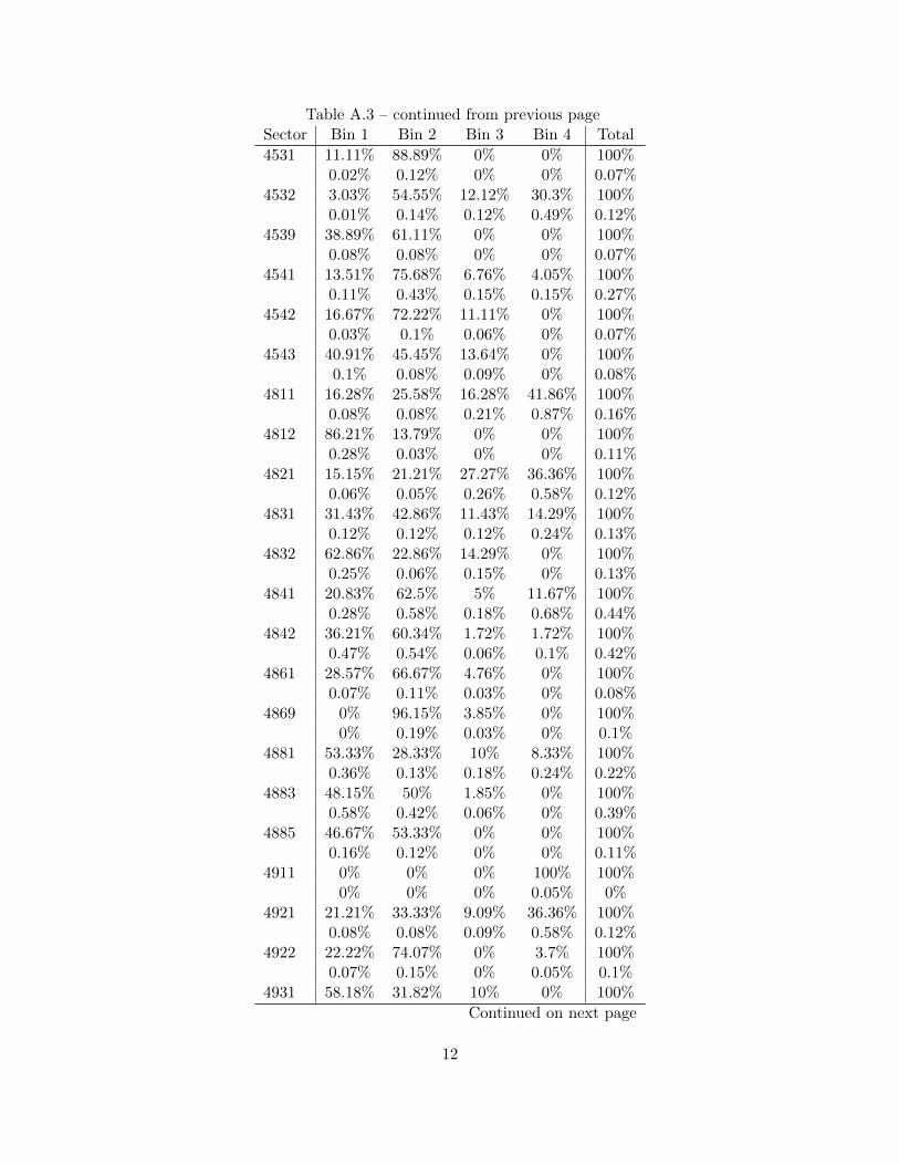
Table A.3 – continued from previous pageSector Bin 1 Bin 2 Bin 3 Bin 4 Total

4531 11.11% 88.89% 0% 0% 100%0.02% 0.12% 0% 0% 0.07%

4532 3.03% 54.55% 12.12% 30.3% 100%0.01% 0.14% 0.12% 0.49% 0.12%

4539 38.89% 61.11% 0% 0% 100%0.08% 0.08% 0% 0% 0.07%

4541 13.51% 75.68% 6.76% 4.05% 100%0.11% 0.43% 0.15% 0.15% 0.27%

4542 16.67% 72.22% 11.11% 0% 100%0.03% 0.1% 0.06% 0% 0.07%

4543 40.91% 45.45% 13.64% 0% 100%0.1% 0.08% 0.09% 0% 0.08%

4811 16.28% 25.58% 16.28% 41.86% 100%0.08% 0.08% 0.21% 0.87% 0.16%

4812 86.21% 13.79% 0% 0% 100%0.28% 0.03% 0% 0% 0.11%

4821 15.15% 21.21% 27.27% 36.36% 100%0.06% 0.05% 0.26% 0.58% 0.12%

4831 31.43% 42.86% 11.43% 14.29% 100%0.12% 0.12% 0.12% 0.24% 0.13%

4832 62.86% 22.86% 14.29% 0% 100%0.25% 0.06% 0.15% 0% 0.13%

4841 20.83% 62.5% 5% 11.67% 100%0.28% 0.58% 0.18% 0.68% 0.44%

4842 36.21% 60.34% 1.72% 1.72% 100%0.47% 0.54% 0.06% 0.1% 0.42%

4861 28.57% 66.67% 4.76% 0% 100%0.07% 0.11% 0.03% 0% 0.08%

4869 0% 96.15% 3.85% 0% 100%0% 0.19% 0.03% 0% 0.1%

4881 53.33% 28.33% 10% 8.33% 100%0.36% 0.13% 0.18% 0.24% 0.22%

4883 48.15% 50% 1.85% 0% 100%0.58% 0.42% 0.06% 0% 0.39%

4885 46.67% 53.33% 0% 0% 100%0.16% 0.12% 0% 0% 0.11%

4911 0% 0% 0% 100% 100%0% 0% 0% 0.05% 0%

4921 21.21% 33.33% 9.09% 36.36% 100%0.08% 0.08% 0.09% 0.58% 0.12%

4922 22.22% 74.07% 0% 3.7% 100%0.07% 0.15% 0% 0.05% 0.1%

4931 58.18% 31.82% 10% 0% 100%

Continued on next page

12

Table A.3 – continued from previous pageSector Bin 1 Bin 2 Bin 3 Bin 4 Total

0.72% 0.27% 0.32% 0% 0.4%5111 24.01% 60.64% 6.93% 8.42% 100%

1.08% 1.89% 0.82% 1.65% 1.48%5112 61.39% 33.66% 2.97% 1.98% 100%

0.69% 0.26% 0.09% 0.1% 0.37%5151 30.06% 62.58% 7.36% 0% 100%

0.55% 0.79% 0.35% 0% 0.6%5152 30% 60% 10% 0% 100%

0.07% 0.09% 0.06% 0% 0.07%5171 0% 3.37% 13.48% 83.15% 100%

0% 0.02% 0.35% 3.59% 0.33%5172 55% 5% 10% 30% 100%

0.12% 0.01% 0.06% 0.29% 0.07%5175 18.75% 42.86% 27.68% 10.71% 100%

0.23% 0.37% 0.91% 0.58% 0.41%5181 52.44% 42.68% 4.88% 0% 100%

0.48% 0.27% 0.12% 0% 0.3%5182 53.52% 46.48% 0% 0% 100%

0.42% 0.25% 0% 0% 0.26%5221 54.48% 36.94% 6.34% 2.24% 100%

1.63% 0.76% 0.5% 0.29% 0.98%5231 45.71% 40.95% 4.76% 8.57% 100%

0.54% 0.33% 0.15% 0.44% 0.38%5239 39.56% 47.25% 3.3% 9.89% 100%

0.4% 0.33% 0.09% 0.44% 0.33%5241 13.77% 21.81% 31.56% 32.86% 100%

1.07% 1.17% 6.47% 11.11% 2.55%5242 28% 56% 14.4% 1.6% 100%

0.39% 0.54% 0.53% 0.1% 0.46%5311 94.6% 5.04% 0% 0.36% 100%

2.94% 0.11% 0% 0.05% 1.02%5312 38.24% 51.96% 5.88% 3.92% 100%

0.44% 0.41% 0.18% 0.19% 0.37%5313 40.82% 54.08% 2.04% 3.06% 100%

0.45% 0.41% 0.06% 0.15% 0.36%5321 28.95% 43.42% 2.63% 25% 100%

0.25% 0.25% 0.06% 0.92% 0.28%5324 16.46% 77.22% 6.33% 0% 100%

0.15% 0.47% 0.15% 0% 0.29%5411 28.43% 59.31% 10.29% 1.96% 100%

0.65% 0.93% 0.62% 0.19% 0.75%5412 48.67% 46.02% 5.31% 0% 100%

0.61% 0.4% 0.18% 0% 0.41%

Continued on next page

13

Table A.3 – continued from previous pageSector Bin 1 Bin 2 Bin 3 Bin 4 Total

5413 52.63% 33.33% 14.04% 0% 100%0.34% 0.15% 0.24% 0% 0.21%

5416 33.87% 61.29% 4.84% 0% 100%0.23% 0.29% 0.09% 0% 0.23%

5418 34.78% 58.7% 6.52% 0% 100%0.18% 0.21% 0.09% 0% 0.17%

5613 23.38% 44.81% 24.68% 7.14% 100%0.4% 0.53% 1.12% 0.53% 0.56%

5615 24.07% 25.93% 48.15% 1.85% 100%0.15% 0.11% 0.76% 0.05% 0.2%

5616 35.53% 18.42% 42.11% 3.95% 100%0.3% 0.11% 0.94% 0.15% 0.28%

5617 36.89% 36.89% 20.49% 5.74% 100%0.5% 0.35% 0.73% 0.34% 0.45%

5621 30% 70% 0% 0% 100%0.03% 0.05% 0% 0% 0.04%

6211 20.13% 54.55% 13.64% 11.69% 100%0.35% 0.65% 0.62% 0.87% 0.56%

6216 25.19% 67.41% 2.96% 4.44% 100%0.38% 0.7% 0.12% 0.29% 0.49%

6221 7.38% 11.07% 27.31% 54.24% 100%0.22% 0.23% 2.18% 7.13% 0.99%

6222 7.32% 19.51% 73.17% 0% 100%0.03% 0.06% 0.88% 0% 0.15%

6223 0% 0% 85.71% 14.29% 100%0% 0% 0.18% 0.05% 0.03%

6231 43.31% 54.78% 0% 1.91% 100%0.76% 0.66% 0% 0.15% 0.57%

6232 77.78% 22.22% 0% 0% 100%0.08% 0.02% 0% 0% 0.03%

7131 0% 88.89% 11.11% 0% 100%0% 0.06% 0.03% 0% 0.03%

7139 31.03% 58.62% 10.34% 0% 100%0.2% 0.26% 0.18% 0% 0.21%

7211 25% 65.87% 7.69% 1.44% 100%0.58% 1.06% 0.47% 0.15% 0.76%

Total 32.71% 47.32% 12.44% 7.53% 100%100% 100% 100% 100% 100%

The table shows the percentage of firms in the PPI that belong to a bin in a givenfour-digit NAICS category (each first line per industry) and the percentage in anindustry given a bin (each second line). Bin 1 groups firms with 1 to 3 goods, bin 2firms with 3 to 5 goods, bin 3 firms with 5 to 7 goods and bin 4 firms with more than7 goods.

14

Table A.4: Variation Explained by Fixed Effects

Products at four-digit level Products at six-digit level Products at eight-digit level

R2 3.20% 10.39% 26.95% 3.20% 13.56% 27.64% 3.20% 15.68% 28.54%Adjusted R2 3.20% 10.39% 25.31% 3.20% 13.47% 25.80% 3.20% 15.48% 26.41%

Month FEs Yes Yes Yes Yes Yes Yes Yes Yes YesProduct FEs No Yes Yes No Yes Yes No Yes YesFirm FEs No No Yes No No Yes No No Yes

We estimate the following specification regarding variation in |∆p|, the absolute size of price changes: |∆p|i,f,p,t =α0{DMonth m}m=12

m=1 +α1DProducti,f,p,t +α2D

Firmi,f,p + εi,f,p,t where i denotes a good, f a firm, p a product at the 4-, 6-, and 8-digit level,

and t time. Dummies are for months, products, and firms.

Table A.5: Relation of Frequency and Number of Goods, Six-Digit Level

Estimated Coefficient

Mean 1.22(0.12)

Median 1.3225% Percentile 0.5975% Percentile 1.80

We estimate the following specification: fj,p =β0,p + β1,pnj,p + εj,p, where fj,p denotes the fre-quency of firm j in a six-digit product categoryp and nj,p the number of goods of that firm. Weestimate the specification at each date, take themedian of β1,p across all products at that date andreport the mean, median and quartiles of medianβ1,p over time.

15

Table A.6: Relation of Absolute Size of Price Changes and Number of Goods, Six-Digit Level

Estimated Coefficient

Mean -0.38(0.026)

Median -0.35825% Percentile -0.52175% Percentile -0.0315

We estimate the following specification: |∆p|j,p =β0,p + β1,pnj,p + εj,p, where |∆p|j,p denotes themean absolute size of price changes of firm j in asix-digit product category p and nj,p the numberof goods of that firm. We estimate the specifi-cation at each date, take the mean of β1,p acrossall products at that date and report the mean,median and quartiles of median β1,p over time.

Table A.7: Fraction of Small Price Changes According to Different Definitions

Number

of Goods |dp| < 12 |dp| |dp| <

13 |dp| |dp| <

14 |dp| |dp| <

110 |dp| |dp| < 1% |dp| < 0.5% |dp| < 0.25%

1-3 39.46% 31.70% 27.28% 17.95% 32.74% 25.78% 20.19%(0.32%) (0.32%) (0.31%) (0.29%) (0.39%) (0.37%) (0.34%)

3-5 44.61% 36.52% 31.74% 21.53% 35.98% 28.81% 22.86%(0.31%) (0.32%) (0.32%) (0.31%) (0.4%) (0.38%) (0.36%)

5-7 47.45% 39.20% 34.80% 23.69% 37.53% 30.15% 23.75%(0.54%) (0.58%) (0.59%) (0.58%) (0.73%) (0.71%) (0.66%)

> 7 50.22% 42.41% 37.56% 26.41% 40.97% 33.40% 26.77%(0.61%) (0.69%) (0.73%) (0.76%) (0.94%) (0.94%) (0.89%)

Pooled 42.93% 34.98% 30.40% 20.44% 34.98% 27.86% 21.98%(0.2%) (0.2%) (0.2%) (0.19%) (0.25%) (0.24%) (0.23%)

The fraction of small price changes is computed in the following way: First, we compute a cut-off that defines a small price change.This is either a fraction of the mean absolute size of price changes |dp| for a given firm, as indicated in the columns, or an absolutepercentage number. Second, we compute the fraction of absolute price changes falling below the cut-off. Third, we summarizemeans across firms within each bin.

16

Table A.8: Marginal Effects for Two-Digit Industries, ± 1/2 Std. Dev., Multinomial Logit

Pooled 1-3 Goods 3-5 Goods 5-7 Goods >7 Goods

Negative Changes

Fraction Industry -0.30% 1.11% 0.68% -0.58% -3.59%Fraction Firm 9.83% 8.13% 8.02% 11.53% 16.22%

Positive Changes

Fraction Industry 0.01% 0.97% 0.25% -1.10% -3.09%Fraction Firm 15.84% 13.57% 13.61% 17.79% 25.73%

The table shows the marginal effects in percentage points of a one-standard deviation change in the explanators

around the mean on the probability of adjusting prices upwards or downwards. Marginal effects are calculated for

the model described in the main text but for each bin separately and with a fraction of same-signed industry-level

price changes defined at the two-digit level. Estimation, given by the separate columns, is for the pooled data and

each bin separately. All reported effects are statistically significantly different from zero.

17

Figure A.1: Mean Frequency Size of Price Changes and Number of Goods, Controlling for Size

19.00%

20.00%

21.00%

22.00%

23.00%

24.00%

25.00%

26.00%

27.00%

28.00%

1-3 3-5 5-7 >7

Mo

nth

ly F

req

uen

cy o

f P

rice

Ch

an

ges

Number of Goods

Monthly Frequency of Price Changes and Number of Goods, Controlling for Firm Size

To obtain the frequency value shown, we estimate the following specification: fi = β0employmenti +∑

k βkDk,i + εi where fi

is the median frequency of price adjustment for a firm i, employment the number of employees of the firm and Dk,i a dummy

for bin k that the firm is in. We then graph βk.

18

Figure A.2: Mean Absolute Size of Price Changes and Number of Goods, Controlling for Size

6.15%

6.65%

7.15%

7.65%

8.15%

8.65%

1-3 3-5 5-7 >7

Mean

Ab

solu

te S

ize o

f P

rice

Ch

an

ges

Number of Goods

Mean Absolute Size of Price Changes and Number of Goods, Controlling for Size

To obtain the mean absolute size of price change values shown, we estimate the following specification: |∆pi| = β0employmenti+∑k βkDk,i + εi where |∆pi| is the median absolute size of price changes for a firm i, employment the number of employees of

the firm and Dk,i a dummy for bin k that the firm is in. We then show βk.

19

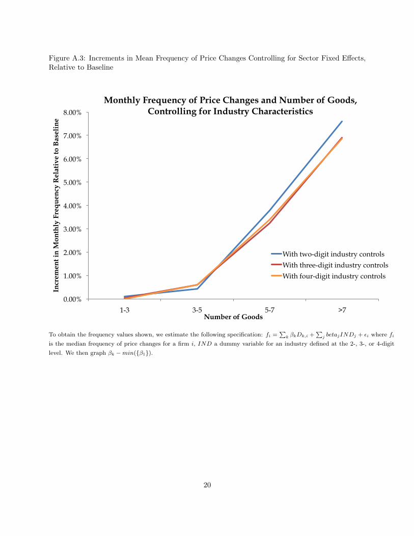
Figure A.3: Increments in Mean Frequency of Price Changes Controlling for Sector Fixed Effects,Relative to Baseline

0.00%

1.00%

2.00%

3.00%

4.00%

5.00%

6.00%

7.00%

8.00%

1-3 3-5 5-7 >7

Incr

em

en

t in

Mo

nth

ly F

req

uen

cy R

ela

tiv

e t

o B

ase

lin

e

Number of Goods

Monthly Frequency of Price Changes and Number of Goods, Controlling for Industry Characteristics

With two-digit industry controls

With three-digit industry controls

With four-digit industry controls

To obtain the frequency values shown, we estimate the following specification: fi =∑

k βkDk,i +∑

j betajINDj + εi where fi

is the median frequency of price changes for a firm i, IND a dummy variable for an industry defined at the 2-, 3-, or 4-digit

level. We then graph βk −min({β1}).

20

Figure A.4: Increments in Mean Absolute Size of Price Changes Controlling for Sector Fixed Effects,Relative to Baseline

0

0.005

0.01

0.015

0.02

0.025

0.03

1-3 3-5 5-7 >7

Mean

Ab

solu

te R

ela

tiv

e S

ize o

f P

rice

Ch

an

ges

Number of Goods

Mean Absolute Size of Price Changes and Number of Goods, Relative to Baseline

With two-digit industry controls

With three-digit industry controls

With four-digit industry controls

To obtain the frequency values shown, we estimate the following specification: |∆pi| =∑

k βkDk,i +∑

j betajINDj + εi where

|∆pi| is the median absolute size of price changes for a firm i, IND a dummy variable for an industry defined at the 2-, 3-, or

4-digit level. We then graph βk −min({β4}).

21

Figure A.5: Mean Frequency of Price Changes and Sectoral Decomposition

10.00%

20.00%

30.00%

40.00%

1-3 3-5 5-7 >7

Mo

nth

ly F

req

uen

cy o

f P

rice

Ch

an

ges

Number of Goods

Monthly Frequency of Price Changes

Sectors 31, 32 ,33

Not sectors 31, 32, 33

We compute the frequency of price changes in exactly the same way as for Figure 1 but with one change: in the last step of

aggregating firm frequencies, we take means for bin-sector group combinations as shown. The two relevant sector groupings are

the two-digit NAICS manufacturing sectors, and all others.

22

Figure A.6: Mean Frequency of Price Changes and Manufacturing Sectors 31, 32, 33

10.00%

20.00%

30.00%

40.00%

1-3 3-5 5-7 >7

Mo

nth

ly F

req

uen

cy o

f P

rice

Ch

an

ges

Number of Goods

Monthly Frequency of Price Changes

Sector 31

Sector 32

Sector 33

We compute the frequency of price changes in exactly the same way as for Figure 1 but with one change: in the last step of

aggregating firm frequencies, we take means for bin-sector combinations as shown. The relevant sectors are the two-digit NAICS

manufacturing sectors 31, 32 and 33.

23

Figure A.7: Mean Absolute Size of Price Changes and Manufacturing Sectors 31, 32, 33

5.00%

6.00%

7.00%

8.00%

9.00%

10.00%

11.00%

1-3 3-5 5-7 >7

Ab

solu

te S

ize o

f P

rice

Ch

an

ges

Number of Goods

Absolute Size of Price Changes

Sectors 31, 32 ,33

Not sectors 31, 32, 33

We compute the absolute size of price changes in exactly the same way as for Figure 4 but with one change: in the last step of

aggregating firm size of price change measures, we take means for bin-sector group combinations as shown. The two relevant

sector groupings are the two-digit NAICS manufacturing sectors, and all others.

24

Figure A.8: Mean Absolute Size of Price Changes and Manufacturing Sectors 31, 32, 33

4.50%

5.50%

6.50%

7.50%

1-3 3-5 5-7 >7

Ab

solu

te S

ize o

f P

rice

Ch

an

ges

Number of Goods

Absolute Size of Price Changes

Sector 31

Sector 32

Sector 33

We compute the absolute size of price changes in exactly the same way as for Figure 4 but with one change: in the last step of

aggregating firm size of price change measures, we take means for bin-sector combinations as shown. The relevant sectors are

the two-digit NAICS manufacturing sectors 31, 32 and 33.

25

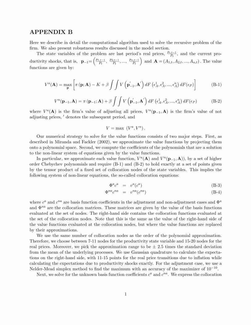
APPENDIX B

Here we describe in detail the computational algorithm used to solve the recursive problem of thefirm. We also present robustness results discussed in the model section.

The state variables of the problem are last period’s real prices,pi,t−1

Pt, and the current pro-

ductivity shocks, that is, p−1=(p1,t−1

Pt,p2,t−1

Pt, ...,

pn,t−1

Pt

)and A = (A1,t, A2,t, ..., An,t) . The value

functions are given by:

V a(A) = maxp

[π (p; A)−K + β

∫ ∫V(p′−1,A

′)dF(ε1A, ε

2A, ..., ε

nA

)dF (εP )

](B-1)

V n(p−1,A) = π (p−1; A) + β

∫ ∫V(p′−1,A

′)dF(ε1A, ε

2A, ..., ε

nA

)dF (εP ) (B-2)

where V a(A) is the firm’s value of adjusting all prices, V n(p−1,A) is the firm’s value of notadjusting prices, ′ denotes the subsequent period, and

V = max (V a, V n) .

Our numerical strategy to solve for the value functions consists of two major steps. First, asdescribed in Miranda and Fackler (2002), we approximate the value functions by projecting themonto a polynomial space. Second, we compute the coefficients of the polynomials that are a solutionto the non-linear system of equations given by the value functions.

In particular, we approximate each value function, V a(A) and V n(p−1,A)), by a set of higherorder Chebychev polynomials and require (B-1) and (B-2) to hold exactly at a set of points givenby the tensor product of a fixed set of collocation nodes of the state variables. This implies thefollowing system of non-linear equations, the so-called collocation equations:

Φaca = va(ca) (B-3)

Φnacna = vna(cna) (B-4)

where ca and cna are basis function coefficients in the adjustment and non-adjustment cases and Φa

and Φna are the collocation matrices. These matrices are given by the value of the basis functionsevaluated at the set of nodes. The right-hand side contains the collocation functions evaluated atthe set of the collocation nodes. Note that this is the same as the value of the right-hand side ofthe value functions evaluated at the collocation nodes, but where the value functions are replacedby their approximations.

We use the same number of collocation nodes as the order of the polynomial approximation.Therefore, we choose between 7-11 nodes for the productivity state variable and 15-20 nodes for thereal prices. Moreover, we pick the approximation range to be ± 2.5 times the standard deviationfrom the mean of the underlying processes. We use Gaussian quadrature to calculate the expecta-tions on the right-hand side, with 11-15 points for the real price transitions due to inflation whilecalculating the expectations due to productivity shocks exactly. For the adjustment case, we use aNelder-Mead simplex method to find the maximum with an accuracy of the maximizer of 10−10.

Next, we solve for the unknown basis function coefficients ca and cna. We express the collocation

1

equations as two fixed-point problems:

ca = Φa−1va(ca) (B-5)

cna = Φna−1vna(cna) (B-6)

and iteratively update the coefficients until the collocation equations are satisfied exactly.Our solution method is standard in the relevant literature for example as in Midrigan (2011).

We still conduct two sensitivity analyses. First, given that zero menu costs imply flex-pricing, weverify that the approximate solution is “good” given the known analytical solution. Figure B.1shows that optimal price policies and the price policies obtained by the approximation line up a45-degree line in this case where we know the exact solution. The norm of the error is of order10−9 and errors are equi-oscillatory, as is a usual property of approximations based on Chebychevpolynomials. Second, we conduct standard stochastic simulations and find that the errors betweenthe left- and right-hand sides of (B-1) and (B-2) at points other than the collocation nodes are onaverage of the order of 10−5 or less.

Figure B.1: Analytical and Numerical Optimal Flex Price

We compute the numerical solution for optimal adjustment prices given productivity shocks and

zero menu costs. We compare to the analytical solution known in the flex price case. Errors are of

the order of 10−9.

2

Table B.1: Results of Simulation: No Correlation, Economies of Scope

1 Good 2 Goods 3 Goods

Frequency of price changes 13.89% 19.16% 20.22%Size of absolute price changes 5.42% 4.37% 4.02%Size of positive price changes 5.53% 4.53% 4.26%Size of negative price changes -5.26% -4.12% -3.66%Fraction of positive price changes 62.92% 60.46% 59.33%Fraction of small price changes 2.41% 20.62% 23.77%Kurtosis 1.45 1.75 1.991st Percentile -7.24% -7.84% -8.34%99th Percentile 7.45% 8.16% 8.96%

Synchronization measures:Fraction, Upwards Adjustments - 30.22 38.05Fraction, Downwards Adjustments - 29.39 37.04

Correlation coefficient - 0 0Menu cost 0.40% 0.70% 0.80%

We perform stochastic simulation of our model in the 1-good, 2-good and 3-goodcases and record price adjustment decisions in each case. Then, we calculatestatistics for each case as described in the text. In the 2-good and the 3-goodcases, we report the mean of the good-specific statistics. We obtain the synchro-nization measure from a multinomial logit regression analogous to the empiricalmultinomial logit regression. We control for inflation. Menu costs are given as apercentage of steady state revenues.

3

Table B.2: Results of Simulation: Correlation, No Economies of Scope

1 Good 2 Goods 3 Goods

Frequency of price changes 13.89% 17.70% 13.93%Size of absolute price changes 5.42% 4.54% 4.87%Size of positive price changes 5.53% 4.71% 5.21%Size of negative price changes -5.26% -4.30% -4.35%Fraction of positive price changes 62.92% 61.11% 61.36%Fraction of small price changes 2.41% 21.38% 24.11%Kurtosis 1.45 1.77 2.031st Percentile -7.24% -8.11% -9.79%99th Percentile 7.45% 8.64% 10.37%

Synchronization measures:Fraction, Upwards Adjustments - 31.44 39.16Fraction, Downwards Adjustments - 30.83 38.16

Correlation coefficient - 0.65 0.65Menu cost 0.40% 0.80% 1.20%

We perform stochastic simulation of our model in the 1-good, 2-good and 3-goodcases and record price adjustment decisions in each case. Then, we calculatestatistics for each case as described in the text. In the 2-good and the 3-goodcases, we report the mean of the good-specific statistics. We obtain the synchro-nization measure from a multinomial logit regression analogous to the empiricalmultinomial logit regression. We control for inflation. Menu costs are given as apercentage of steady state revenues.

4

Table B.3: Results of Simulation: No Correlation, No Economies of Scope

1 Good 2 Goods 3 Goods

Frequency of price changes 13.89% 16.25% 13.93%Size of absolute price changes 5.42% 4.49% 4.87%Size of positive price changes 5.53% 4.66% 5.21%Size of negative price changes -5.26% -4.23% -4.35%Fraction of positive price changes 62.92% 61.86% 61.36%Fraction of small price changes 2.41% 21.13% 24.11%Kurtosis 1.45 1.81 2.031st Percentile -7.24% -8.01% -9.79%99th Percentile 7.45% 8.54% 10.37%

Synchronization measures:Fraction, Upwards Adjustments - 30.33 38.40Fraction, Downwards Adjustments - 29.43 37.11

Correlation coefficient - 0 0Menu cost 0.40% 0.80% 1.20%

We perform stochastic simulation of our model in the 1-good, 2-good and 3-goodcases and record price adjustment decisions in each case. Then, we calculatestatistics for each case as described in the text. In the 2-good and the 3-goodcases, we report the mean of the good-specific statistics. We obtain the synchro-nization measure from a multinomial logit regression analogous to the empiricalmultinomial logit regression. We control for inflation. Menu costs are given as apercentage of steady state revenues.

5

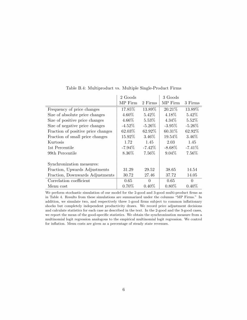
Table B.4: Multiproduct vs. Multiple Single-Product Firms

2 Goods 3 GoodsMP Firm 2 Firms MP Firm 3 Firms

Frequency of price changes 17.85% 13.89% 20.21% 13.89%Size of absolute price changes 4.60% 5.42% 4.18% 5.42%Size of positive price changes 4.66% 5.53% 4.34% 5.52%Size of negative price changes -4.52% -5.26% -3.95% -5.26%Fraction of positive price changes 62.03% 62.92% 60.31% 62.92%Fraction of small price changes 15.92% 3.46% 19.54% 3.46%Kurtosis 1.72 1.45 2.03 1.451st Percentile -7.94% -7.42% -8.68% -7.41%99th Percentile 8.36% 7.56% 9.04% 7.56%

Synchronization measures:Fraction, Upwards Adjustments 31.29 29.52 38.65 14.54Fraction, Downwards Adjustments 30.72 27.46 37.72 14.05

Correlation coefficient 0.65 0 0.65 0Menu cost 0.70% 0.40% 0.80% 0.40%

We perform stochastic simulation of our model for the 2-good and 3-good multi-product firms asin Table 4. Results from these simulations are summarized under the columns “MP Firms.” Inaddition, we simulate two, and respectively three 1-good firms subject to common inflationaryshocks but completely independent productivity draws. We record price adjustment decisionsand calculate statistics for each case as described in the text. In the 2-good and the 3-good cases,we report the mean of the good-specific statistics. We obtain the synchronization measure from amultinomial logit regression analogous to the empirical multinomial logit regression. We controlfor inflation. Menu costs are given as a percentage of steady state revenues.

6

APPENDIX C

In this appendix, we describe in further detail the sampling procedure of the BLS which impliesa monotonic relationship between the actual and sampled number of goods produced by multi-product firms. First, we document that firms with more goods have larger total sales. More goodswill therefore be sampled in total from large firms. Second, we show that sales shift to goods withlower sales rank in firms with more goods. Therefore, standard survey design implies that not onlymore, but different goods will be sampled from larger firms. Finally, we also summarize the fractionof joint price changes in firms.

Sales ValuesFirst, we document that firms with more goods have larger total sales in the data. Because total

sales value determines the sampling probabilities of firms in the sampling selection procedure,11

this implies that on average more goods will therefore be sampled from large firms.We compute our measure of total sales value for each n-good-type firm in the following way.

First, we compute the total dollar-value sales in a given month, year, and firm by aggregating upthe item dollar-value of sales from the last time the item was re-sampled. Second, we count thenumber of goods for each firm in a given month and year. Third, we compute the unweighted andweighted median total sales value across all firms for a given n-good type of firm and month andyear. Fourth, we calculate the mean and median sales value for an n-good type of firm

We find that firms with more goods have larger total sales: there is a strong empirical, monotonicrelationship between the number of goods and the natural logarithm of the total sales. Figure C.1summarizes this relationship. Because total sales value determines the sampling probabilities offirms in the BLS sampling selection procedure, on average a higher number of goods will be collectedfrom large firms.

Within-Firm Sales SharesSecond, we show that sales shift to goods with lower sales rank in firms with more goods.

Therefore, standard survey design such as sampling proportional to size implies that not onlymore, but different goods will likely be sampled from larger firms.

We compute within-firm sales shares and sales ranks in the following way. First, we compute thetotal dollar-value sales for a given month, year, and firm by aggregating up the dollar-value of salesof the good from the last time the item was re-sampled. Second, we calculate the good-specific salesshares for each firm in a given month and year. Third, we rank the goods in each firm according tothese sales shares. Fourth, we count the number of goods for each firm in a given month and year.Fifth, we compute the mean sales shares for an r-ranked good in an n-good firm in a given monthand year, across all firms. Sixth, we compute the sales-weighted mean for an r-ranked good inan n-good firm over time. These calculations give us the sales share representative of an r-rankedgood in a firm with n goods.12

We find that sales shift to goods with lower sales rank in firms with more goods. For example,the representative sales share of the best-selling good in a two-good firm is 63% while it is 45%for the second good. For a three-good firm, the sales shares are 45%, 35%, and 30%. Table C.1

11Employment is another measure of firm size. The exact same results hold for employment: firms with more goodshave a larger number of employees.

12Note that these shares do not have to sum up to 100% in an n-good firm by way of computation.

1

summarizes sales shares by the number of goods and rank of the goods. The table covers firmswith up to 11 goods which account for more than 98% of all prices in the data. Under standardsurvey designs such as sampling proportional to size and a fixed survey budget not only more, butdifferent goods are more likely to be sampled when firms produce more goods.

16

16.5

17

17.5

18

18.5

19

19.5

20

20.5

21

1 2 3 4 5 6 7 8 9 10 11

Lo

g M

ean

Sal

es V

alu

e

Number of Goods

Log Mean Firm Sales Value by Number of Goods

Figure C.1: Log Mean Firm Sales Value by Number of Goods

2

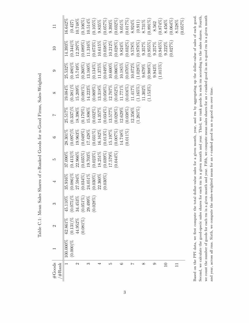
Tab

leC

.1:

Mea

nS

ales

Sh

ares

ofr-

Ran

ked

Good

sfo

rn

-Good

Fir

ms,

Sal

es-W

eigh

ted

#G

ood

s1

23

45

67

89

1011

/#

Ran

k 110

0.0

00%

62.8

61%

45.

110%

35.9

16%

37.0

90%

28.3

01%

25.5

17%

19.0

84%

25.5

32%

14.3

93%

16.6

42%

(0.0

00)

%(0

.131

)%(0

.075

)%(0

.086

)%(0

.413

)%(0

.097

)%(0

.337

)%(0

.381

)%(0

.480

)%(0

.344

)%(0

.427

)2

44.9

52%

34.

453%

27.5

94%

22.9

66%

19.9

63%

18.3

96%

15.2

09%

15.7

49%

12.2

97%

10.7

48%

(0.0

81%

)(0

.051

%)

(0.0

34%

)(0

.035

%)

(0.0

49%

)(0

.170

%)

(0.0

91%

)(0

.260

%)

(0.0

89%

)(0

.106

%)

329

.499

%24

.051

%19

.703

%17

.428

%15

.896

%14

.223

%13

.160

%11

.316

%10

.514

%(0

.028

%)

(0.0

30%

)(0

.023

%)

(0.0

31%

)(0

.032

%)

(0.0

69%

)(0

.134

%)

(0.0

73%

)(0

.105

%)

422

.360

%18

.251

%16

.162

%14

.357

%13

.318

%11

.375

%10

.615

%9.

835%

(0.0

30%

)(0

.039

%)

(0.0

13%

)(0

.034

%)

(0.0

50%

)(0

.049

%)

(0.0

38%

)(0

.057

%)

517

.579

%15

.197

%13

.577

%12

.707

%10

.600

%10

.212

%9.

393%

(0.0

44%

)(0

.007

%)

(0.0

28%

)(0

.052

%)

(0.0

66%

)(0

.028

%)

(0.0

32%

)6

14.7

48%

12.6

29%

11.7

71%

10.1

85%

9.82

4%9.

051%

(0.0

11%

)(0

.038

%)

(0.0

16%

)(0

.070

%)

(0.0

32%

)(0

.017

%)

712

.356

%11

.417

%10

.072

%9.

578%

8.92

4%(1

.261

%)

(1.1

65%

)(1

.028

%)

(0.9

78%

)(0

.911

)8

11.3

02%

9.67

9%9.

357%

8.73

1%(1

.153

%)

(0.9

88%

)(0

.955

%)

(0.8

91%

)9

9.94

3%9.

257%

8.56

2(1

.015

%)

(0.9

45%

)(0

.874

%)

109.

222%

8.45

6%(0

.027

%)

(0.0

64%

)11

8.52

8%(0

.057

%)

Base

don

the

PP

Idata

,w

efirs

tco

mpute

the

tota

ldollar-

valu

esa

les

for

agiv

enm

onth

,yea

r,and

rmby

aggre

gati

ng

up

the

dollar-

valu

eof

sale

sof

each

good.

Sec

ond,

we

calc

ula

teth

egood-s

pec

icsa

les

share

sfo

rea

chrm

ina

giv

enm

onth

and

yea

r.T

hir

d,

we

rank

goods

inea

chrm

acc

ord

ing

toth

esa

les

share

s.F

ourt

h,

we

count

the

num

ber

of

goods

for

each

rmin

agiv

enm

onth

and

yea

r.F

ifth

,w

eco

mpute

mea

nsa

les

share

sfo

ranr-

ranked

good

inann

-good

rmin

agiv

enm

onth

and

yea

r,acr

oss

all

rms.

Six

th,

we

com

pute

the

sale

s-w

eighte

dm

ean

for

anr-

ranked

good

inann

-good

rmov

erti

me.

3