multiprocessor scheduling with communication delays · multiprocessor scheduling with communication...
TRANSCRIPT

Multiprocessor scheduling with communication delays
Veltman, B.
DOI:10.6100/IR396672
Published: 01/01/1993
Document VersionPublisher’s PDF, also known as Version of Record (includes final page, issue and volume numbers)
Please check the document version of this publication:
• A submitted manuscript is the author's version of the article upon submission and before peer-review. There can be important differencesbetween the submitted version and the official published version of record. People interested in the research are advised to contact theauthor for the final version of the publication, or visit the DOI to the publisher's website.• The final author version and the galley proof are versions of the publication after peer review.• The final published version features the final layout of the paper including the volume, issue and page numbers.
Link to publication
General rightsCopyright and moral rights for the publications made accessible in the public portal are retained by the authors and/or other copyright ownersand it is a condition of accessing publications that users recognise and abide by the legal requirements associated with these rights.
• Users may download and print one copy of any publication from the public portal for the purpose of private study or research. • You may not further distribute the material or use it for any profit-making activity or commercial gain • You may freely distribute the URL identifying the publication in the public portal ?
Take down policyIf you believe that this document breaches copyright please contact us providing details, and we will remove access to the work immediatelyand investigate your claim.
Download date: 24. Jul. 2018

MULTIPROCESSOR SCHEDULING WITH
COMMUNICATION DELAYS
Bart Veltman

MULTIPROCESSOR SCHEDULING WITH
COMMUNICATION DELAYS

MULTIPROCESSOR SCHEDULING WITH
COMMUNICATION DELAYS
Proefschrift ter verkrijging van de graad van doctor aan de
Technische Universiteit Eindhoven, op gezag van de Rector Magnificos, prof. dr. J.H. van Lint, voor een commissie aangewezen door bet College van
Dekanen in bet openbaar te verdedigen op dinsdag 18 mei 1993 te 16.00 uur
door
Bart Veltman
geboren te Reinheim (BRD)
1993 CWI, Amsterdam

Dit proefschrift is goedgekeurd door de promotor:
prof. dr. J. K. Lenstra.

Acknowledgements
The work presented here has been carried out at the CWI in Amsterdam as part of the ScheduLink subproject within the Par Tool project. The ParTool project is partially supported by SPIN, a Dutch computer science stimulation program.
I am truly grateful to my supervisor, Jan Karel Lenstra, and my other coauthors, Han Hoogeveen, Ben Lageweg, Steef van de Velde en Marinus Veldhorst. I have learned a lot from their expertise. Working together has been a great pleasure.
Bart Veltman

Voor Hanna, Rob, Dirkje en Dineke

Table of contents

Multiprocessor scheduling with communication delays
1. Introduction 1
2. A general model for parallel processor scheduling 7 2.1. The processor model 8 2.2. The program model 8 2.3. Communication 10 2.4. Task duplication 11 2.5. Classification and notation 12
2.5.1. Processor environment 12 2.5.2. Task characteristics 13 2.5.3. Optimality criterion 14
2.6. Literature review 14 2.6.1. Single-processor tasks and communication delays 15 2.6.2. Multiprocessor tasks 20
3. Communication delays 27 3 .1. The restricted variant 29 3.2. The unrestricted variant 32 3.3. A dynamic programming formulation 36 3.4. Trees 38 3.5. Two open problems 40
4. Task duplication 43 4.1. The potential profit 44
5. Multiprocessor tasks with prespecified processor allocations 47 5.1.Makespan 48
5 .1.1. Three processors and the block constraint 49 5.1.2. Strong NP-hardness for the general3-processor problem 52 5 .1.3. Unit execution times, release dates, and precedence constraints 54
5.2. Sum of completion times 57 5.2.1. NP-hardness for the 2-processor problem 58 5 .2.2. Strong NP-hardness for the general3-processor problem 61 5.2.3. Unit execution times and precedence constraints 61
6. Chains oflength 1, or the two-stage flow shop 6.1. Ordinary NP,.hardness 6.2. Strong NP-hardness
63 65 66

Table of contents
7. Tosca: methodology 69 7 .1. The problem type 70 7 .2. The solution method 71 7.3. Priority rules, evaluation rule, and lower bound rule 7 4 7 .4. Lower bounds on the makespan 77
8. Tosca: implementation 79 8.1. Input and output specification 80 8.2. User interface and functional description 82
8.2.1. The main menu 83 8.2.2. The schedule menu 83 8.2.3. The task priority menu 84 8.2.4. The processor priority menu 84 8.2.5. The evaluation rule menu 85 8.2.6. The lower bound rule menu 85 8.2. 7. The view menu 85 8.2.8. The problem menu 85 8.2.9. The last schedule menu 85 8.2.10. The best schedule menu 86 8.2.11. The previous schedule menu 86 8.2.12. The lower bounds menu 86 8.2.13.Thesavemenu 86 8.2.14. The preempt menu 86 8.2.15.Theresumemenu 86
8.3. Four problem generators 86 8.3.1. The generator for layered precedence relations 87 8.3.2. The generator for series-parallel precedence relations 88 8.3.3. The generator for arbitrary precedence relations 89 8.3.4. The generator for prespecified precedence relations 89
8.4. Computational results 90 8.4.1. List scheduling 92 8.4.2. Searching with d =t =u =2 96 8.4.3. Searching with d=t=u =3 97
9. Tosca: an example 99
References 105
Samenvatting 111

1. Introduction

2 Multiprocessor scheduling with communication delays
From the late fifties onwards, many architectures for parallel computers have been proposed. Some models are useful from a theoretical point of view, but their realization is generally not feasible due to physical limitations; their main purpose is to help to design and analyze parallel algorithms. Others are more realistic and exist or are being built. Unfortunately, multiprocessors strongly differ from each other and, accordingly, there exists no general model that effectively describes the broad spectrum of feasible parallel architectures. Different classification schemes have been proposed, based on processor autonomy [Flynn, 1966], interprocessor communication [Schwartz, 1980], and mode of operation [Treleaven, Brownbridge, and Hopkins, 1982]. The diversity of models and existing architectures causes a series of problems when one wishes to take advantage of the computing power that multiprocessors offer. These problems can be summarized as follows. Important for programming a parallel computer is to preserve an algorithm's intrinsic parallelism when formalized in a programming language, to properly partition a program into tasks, and to assign the tasks to processors while respecting the information dependencies in between the tasks.
This thesis concerns the latter aspect: the new allocation and scheduling problems that have to be solved. These problems differ from the problems of classical sequencing and scheduling theory mainly in that interprocessor communication delays have to be taken into account.
In the literature, we distinguish two basically different approaches to handle communication delays. The first approach formulates the problem in graph theoretic terms; one speaks of the mapping problem (Bokhari, 1981]. The program graph is regarded as an undirected graph, where the vertices correspond to tasks and an (undirected) edge indicates that the adjacent tasks interact, that is, communicate with each other. The multiprocessor architecture is also regarded as an undirected graph, with nodes corresponding to processors. Processors are assigned to tasks. A mapping aims at reducing the total interprocessor communication time and balancing the workload of the processors, thus attempting to find an allocation that minimizes the overall completion time.
The second approach considers the allocation problem as a pure scheduling problem. It regards the program graph as an acyclic directed graph. Again, the vertices represent the tasks, but a (directed) arc indicates a one-way communication between a predecessor task and a successor task. A schedule is an allocation of each task to a time interval on one or more processors such that, among others, precedence constraints and communication delays are taken into account. It aims at minimizing the maximum or the average task

1. Introduction 3
completion time. We will take this second approach. Eventually, it may be desirable to combine the mapping approach and the
scheduling approach when allocating a parallel program to a multiprocessor. In that case, the combined approach would first schedule the tasks on a virtual architecture graph and next find a mapping of the virtual architecture graph onto the physical architecture of the multiprocessor [Kim, 1988].
Following the second approach, we address the allocation problems in the context of deterministic machine scheduling theory. Scheduling theory in general is concerned with the optimal allocation of scarce resources (processors) to activities (tasks) over time. The problems we consider are deterministic in the sense that all the information that defines an instance is known with certainty in advance. A complete formulation of the problem type to be considered in this thesis is given in Chapter 2.
Deterministic scheduling theory is part of the area of combinatorial optimization. Combinatorial optimization involves problems in which we have to choose the best from a discrete and often finite set of alternatives. The finiteness suggests the brute-force approach of complete enumeration to be effective: simply generate all feasible solutions, examine their costs, and select the best one. However, for realistic problems the time requirements of this method are prohibitive and we have to search for faster algorithms. The fundamental question is whether there exists an algorithm that solves a given problem to optimality in polynomial time. Algorithms that run in polynomial time are considered to be 'fast', and problems for which such an algorithm exists are said to be 'well-solved'. For other problems it has been shown that the existence of a polynomial-time algorithm is highly unlikely; these are the NP-hard problems. Complexity theory provides a mathematical framework in which computational problems can be classified as being solvable in polynomial time or NP-hard. The reader is referred to the textbook by Garey and Johnson [1979] for a detailed treatment of the subject. The complexity of many scheduling problems that come up in the context of programming a parallel computer is dealt with in Chapters 3-6. We will now give an overview ofthese chapters.
As indicated before, interprocessor communication delays form a major problem when one is programming a multiprocessor. Each task of a parallel program produces information which is in whole or in part required by one or more other tasks. The transmittal of information may induce several sorts of communication delays, depending on the amount of the information that is transferred. In Chapter 3, we study the simplest model that allows for communication delays: a set of unit-time tasks has to be processed subject to

4 Multiprocessor scheduling with communication delays
precedence constraints and unit-time communication delays. We consider two cases, in which the number of processors is restricted and unrestricted, respectively. For either case, we investigate the question whether there exists a schedule of length at most equal to a given threshold value. We also show that dynamic programming gives a polynomial-time algorithm in case the width of the precedence relation is fixed, i.e., part of the problem type. Finally, we show NP-hardness for the case that the precedence relation can be represented by a directed tree.
Communication delays may be reduced or even avoided by task duplication, that is, the creation of copies of a task. In Chapter 4, we investigate the trade-off between the optimal makespan of schedules with and without duplicated tasks. In general, task duplication can decrease the schedule length by a factor at most equal to the number of processors, even for tree-type precedence relations. However, in case of unit-time processing requirements and unit-time communication delays task duplication can help a factor of two, but no more.
Another aspect of multiprocessor scheduling is that a task may require more than one processor for its execution. Such tasks are referred to as multiprocessor tasks. In Chapter 5 we investigate the computational complexity of scheduling multiprocessor tasks with prespecified processor allocations. Moreover, we investigate the complexity when various additional task characteristics are involved, such as precedence constraints and release dates.
In Chapter 6 we explore a hybrid variant, in which some tasks are to be allocated to either of two processors and others have a prespecified allocation to a single processor. The multiprocessor architecture is a two-stage pipeline, where the first stage consists of two independent identical processors and the second stage consists of a single processor. This problem can be viewed as an extension of the classical two-stage flow shop problem. We establish its NPhardness in the strong sense.
The general model described in Chapter 2 involves multiprocessor tasks, possibly with prespecified processor allocations, and allows for communication delays and task duplication. From the analyses of Chapters 3-6, we may conclude that it is unlikely that fast algorithms exist that solve the scheduling problem in its most general form to optimality. One is confined to take an approximative approach. Tosca, our tunable off-line scheduling algorithm, embodies such an approach. It has been developed as a tool to support the scheduling of parallel programs on distributed memory architectures. Tosca' s purpose is to assist in the design and analysis of schedules of a given

1. Introduction 5
computation graph on a given processor model, allowing for communication delays. Tosca can be used to obtain performance predictions with respect to a program under development; given a decomposition of such a program, a schedule measures its quality.
Tosca constructs schedules for instances that may consist of multiprocessor tasks, possibly with prespecified processor allocations. It allows for communication delays, but does not apply task duplication. Tasks may be grouped into families. Tasks that belong to the same family must be executed by the same collection of processors. Tosca tries to find a reasonable solution in a reasonable amount of time by bounded enumeration. In principle, a schedule can be constructed by iteratively selecting the next task to schedule, allocating a collection of processors to it, and starting the task as early as possible on that collection. The various possible choices can be represented by an enumeration tree. The process of bounded enumeration considers only part of this enumeration tree. It consists of a number of stages. At each stage a task and a processor allocation for that task are selected. In order to select this task and allocation, Tosca generates a subtree of the enumeration tree. The subtree is determined by three parameters (which control the width and the depth of the subtree), two priority rules (for choosing good tasks and allocations), and a lower bound rule (in order to eliminate unpromising branches). The leaves of the subtree are evaluated according to an evaluation rule. A task-allocation pair that leads to a leaf of minimum value is selected. Tosca is tunable, since it enables the user to control the speed of the solution method and the quality of the schedules produced. First, by adjusting the three parameters the user influences the size of the subtree that is computed. Second, the user has to define two priority rules; one for selecting tasks and another for selecting processors. These rules may be part of a given set of rules or are of the user's making. Third, the user has to specify a lower bound rule and an evaluation rule. A detailed description of Tosca' s methodology is given in Chapter 7.
Tosca is equipped with a simple user interface. All the information is presented in alphanumerical manner. The man-machine interaction is menu driven, so that at any moment all feasible commands are visible. Tosca's implementation is described in Sections 8.1 and 8.2. Together with Section 7.3, these sections can be seen as a manual for the use of Tosca. Tosca has been tested on four classes of problem instances: layered precedence relations, series parallel precedence relations, arbitrary precedence relations, and two precedence relations from practice. In addition to the precedence relations, we generated data sets, processing times, and task sizes. The corresponding four problem generators are described in Section 8.3. For the instances that were

6 Multiprocessor scheduling with communication delays
generated, we applied list scheduling with a number of different priority rules to construct initial schedules. Next we tried to build better schedules by use of bounded enumeration with a more restricted number of priority rules. In Section 8.4 we report on these experiments.
As an illustration of the models and methodology described in this thesis, especially those concerning Tosca, we present a small example in Chapter 9. Amongst others, it illustrates the aspects of communication delays, multiprocessor tasks, list scheduling and bounded enumeration.
Chapter 2 is a substantial revision and extension of: B. Veltman, B.J. Lageweg, J.K. Lenstra (1990). Multiprocessor scheduling
with communication delays. Parallel Comput.J6, 173-182.
Chapter 3 is based on: J.A. Hoogeveen, J.K. Lenstra, B. Veltman (1992). Three,four, five, six, or the
complexity of scheduling with communication delays, Report BS-R9229, CWI, Amsterdam;
J.K. Lenstra, M. Veldhorst, B. Veltman (1993). The complexity of scheduling trees with communication delays, in preparation.
Chapter 5 is based on: J.A. Hoogeveen, S.L. van de Velde, B. Veltman (1993). C?mplexity of
scheduling multiprocessor tasks with prespecified processor allocations. Discrete Appl. Math., to appear.
Chapter 6 is based on: J.A. Hoogeveen, J.K. Lenstra, B. Veltman (1993). Minimizing makespan in a
multiprocessor flow shop is strongly NP-hard, in preparation.
Chapters 7 through 8 are based on: B. Veltman, B.J. Lageweg, J.K. Lenstra (1993). Tosca: a tunable off-line
scheduling algorithm, in preparation.

2. A general model for parallel processor scheduling

8 2. A general model for parallel processor scheduling
As indicated in Chapter 1, the subject of this thesis is the study of the allocation of program modules or tasks to parallel processors in the context of deterministic machine scheduling theory. A multiprocessor architecture can be represented by an undirected graph. Tasks can be processed on various subgraphs of the multiprocessor graph. Data dependencies define a precedence relation on the task set. The transmittal of data may induce several sorts of communication delays. These delays may be reduced or even avoided by task duplication. We search for an allocation of tasks to processors that minimizes the maximum or total completion time.
In this chapter, we formulate our scheduling model, we propose a classification that extends the scheme of Graham, Lawler, Lenstra and Rinnooy Kan [1979], and we review the available literature.
2.1. The processor model The multiprocessor chosen consists of a collection of m processors, each provided with a local memory and mutually connected by an intercommunication network. The multiprocessor architecture can be represented by an undirected graph. Several examples are given in Figure 2.1; cf. Kindervater and Lenstra [1988]. The nodes of such a graph correspond to the processors of the architecture it represents. Transmitting data from one processor to another is considered as an independent event, which does not influence the availability of the processors on the transmittal path. In case of a shared memory, the assumption of having local memory only overestimates the communication delays.
2.2. The program model A parallel program is represented by means of an acyclic directed graph. The nodes of this program graph correspond to the modules in which the program is decomposed; they are called tasks. Each task produces information, which is in whole or in part required by one or more other tasks. These data dependencies impose a precedence relation on the task set; that is, whenever a task requires information, it has to succeed the tasks that deliver this information. The arcs of the graph represent these precedence constraints. The transmittal of information may induce several sorts of communication delays, which will be discussed in the next section. Task duplication, that is, the creation of copies of a task, might reduce such communication delays. Task duplication is discussed in Section 2.4.
The task set is partitioned into a number of families. Each task belongs to exactly one family. A task can be processed on various subgraphs of the

2.2. The program model
(i) Complete network. (ii) Mesh connected network
(iii) Perfect shuffle network
( iv) Cube connected ( v) Cube connected cycles network. network.
(vi) Master-slave network
(vii) Binary trees network
Figure 2.1. Seven interconnection networks.
9
multiprocessor graph. Tasks that belong to the same family have to be executed by the same subgraph of the multiprocessor graph. We assume that for each family a collection of subgraphs on which its tasks can be processed is specified, and that for each task in that family and each of its subgraphs a corresponding processing time is given. If the processors of the architecture are identical, then for each ta.<;k the processing times related to isomorphic subgraphs are equal. For instance, one may think of a collection of

10 2. A general model for parallel processor scheduling
subhypercubes of a hypercube system of processors, or a collection of submeshes of a mesh connected system. Another possibility occurs when each task can be processed on any sub graph of a given family-dependent size.
If preemption is allowed, then the processing of any operation may be interrupted and resumed at a later time. Although task splitting may induce communication delays, it may also decrease the cost of a schedule with respect to one or more criteria. We will not explore the aspect of communication delays that are induced by preemption in detail, but concentrate on communication delays between precedence-related tasks.
2.3. Communication The information a task needs (or produces) has to be (or becomes) available on all the processors handling this task. The size of this data determines the communication times.
If two tasks Jk and 11 both succeed a task Jj, then they might partly use the same information from task Jj. Under the condition that the memory capacity of a processor is adequate, only one transmission of this common information is needed if Jk and 11 are scheduled on the same subgraph of the multiprocessor graph. It is therefore important to determine the data set a task needs from each of its predecessors. The transfer of data between Jj and h can be represented by associating a data set with the arc (Jj,Jk) of the transitive closure of the program graph. This would generally lead to the specification of 8(n2) sets, if there are n tasks. Another possibility is to associate two sets Ij and Oi with each task Jj, representing the data that this task requires and delivers, respectively. This requires 8(n) sets. The intersection 0/1/k gives the data dependency of tasks Jj and Jk.
Each information set has a weight, which is specified by a function c : 2D ~N. where D is the set containing all information. This function gives the time needed to transmit data from one processor to another, regarded as independent of the processors involved. Let Ue 2D be a data set and let { U 1, U 2 , ••• , U u } be a partition of U. We assume that U can be transmitted in such a way that uf=1 Ui is available when a time period of length at most c(u~=I Ui) has elapsed, for each t with l~t~u. We also assume that c(0)=0 and that c (U) ~ c (W) for all U c We 2D. These conditions state that a data set U can be transmitted in such a way that a subset of U becomes available no later than when this subset would be transmitted on its own.

2.4. Task duplication 11
Jk I h P(k, 2) U(2, l,k) c(U(2, l,k))
h {a,b} {2} {a,b} 2
J3 I
{a,c} {2,3} { a,b,c} 5
Mzb @EJ Mt 1
------0 2 4 7
Figure 2.2. Communication delays.
Interprocessor communication occurs when a task Jk needs information from a predecessor Ji and makes use of at least one processor that is not used by Ji. Let Mi be such a processor. Let F (j) denote the set of successors of Ji and, given a schedule, let P (k, i) denote the set of tasks scheduled on M1 before and including Jk. Prior to the execution of Jb the data set U(i,j,k)=UleF(j)rJ'(k,i)(Ojf'llt) has to be transmitted to Mi, since not only Jk but also each successor of Ji that precedes Jk on Mi requires its own data set. The time gap in between the completion of Ji (at time Cj) and the start of Jk (at time Sk) has to allow for the transmission of U(i,j,k), as illustrated in Figure 2.2. The communication time is given by c(U(i,j,k)). For feasibility it is required that Sk- Ci ~c (U (i,j,k)). At the risk of laboring the obvious, let it be mentioned that the communication time is schedule-dependent.
Sometimes one wishes to disregard the data sets and simply to associate a communication delay with each pair of tasks. That is, a (predecessor, successor) pair of tasks (Jj,Jk) assigned to different processors needs a communication time of a given duration cik· The communication time is of length ci* if it depends on the broadcasting task only, it is of length c*k if it depends on the receiving task only. Finally, it may be of constant length c, independent of the tasks.
2.4. Task duplication If one manages to execute all predecessors of a task on all of the processors handling that task, then one may reduce or even avoid communication delays. This can be done by task duplication, that is, the creation of copies of a task.
Consider the example given in Figure 2.2. An optimal schedule for these three tasks without duplication takes six time units, whereas an optimal

12 2. A general model for parallel processor scheduling
M2[TI. 1 2
Mt~ 0 2 4 6 0 2 4 6
Figure 2.3. Task duplication.
schedule with task duplication is of length four, as illustrated in Figure 2.3. In the latter, task J 1 is executed twice: once by processor M 1 and once by processor M 2 • This enables tasks J 2 and J 3 to be executed without any form of communication delay; task J 2 receives its information from the copy of task J 1
that is executed by M 2 and J 3 receives its information from the copy of J 1 that is processed by M 1 •
Let Jj and Jk be such that lr~Jk. In a feasible schedule each copy of Jk has to receive the information it needs for processing in time, that is, there has to be a copy of Jj such that the time gap between the completion of this copy of Jj and the start of the copy of Jk allows for the transmission of the required information.
2.5. Classification In general, m processors Mi ( i == 1, ... , m) have to process n tasks Jj ( j == 1, ... , n ). A schedule is an allocation of (each copy of) a task to a time interval on one or more processors. A schedule is feasible if no two of these time intervals on the same processor overlap and if, in addition, it meets a number of specific requirements concerning the processor environment and the task characteristics (e.g., precedence constraints and communication delays). A schedule is optimal if it minimizes a given optimality criterion. The processor environment, the task characteristics and the optimality criterion that together define a problem type, are specified in terms of a three-field classification a I ~I y, which is specified below. Let o denote the empty symbol.
2.5 .1. Processor environment The first field a== a 1 a 2 specifies the processor environment. The characterization a 1 =P indicates that the processors are identical parallel processors. The characterization P indicates that, in addition, the number of processors is not restricted; e.g., m ~ n is sufficient in case of single-processor tasks.
If a2 is a positive integer, then m is a constant, equal to a2 ; it is specified as

2.5. Classification 13
part of the problem type. If az = o, then m is a variable, the value of which is specified as part of the problem instance.
2.5.2. Task characteristics The second field ~ c { ~ 1 , ••. , ~8 } indicates a number of task characteristics, which are defined as follows. 1. ~1 E {prec,tree,chain, o }.
~~ =prec: A precedence relation ~is imposed on the task set due to data dependencies. It is denoted by an acyclic directed graph G with vertex set { 1, ... , n}. If G contains a directed path from j to k, then we write Jj~h and require that Jj has been completed before J k can start. ~ 1 =tree: G is a rooted tree with either outdegree at most one for each vertex or indegree at most one for each vertex. ~1 chain: G is a collection of vertex-disjoint chains. ~ 1 o: No data dependencies occur, so that the precedence relation is empty.
2. ~2 E {com,cjk•cj*•c*k•c,c=l,o} This characteristic concerns the communication delays that occur due to data dependencies. To indicate this, one has to write ~ directly after ~ 1 •
~ =com: Communication delays are derived from given data sets and a given weight function, as described in Section 2.3. In all the other cases, the communication delays are explicitly specified. ~2 = cjk: Whenever Jj~h and Jj and Jk are assigned to different processors, a communication delay of a given duration cjk occurs. ~ The communication delays depend on the broadcasting task only. ~ = c*k: The communication delays depend on the receiving task only. ~2 = c: The communication delays are equal. ~2 Each communication delay takes unit time. ~2 =o: No communication delays occur (which does not imply that no data dependencies occur).
3. ~3 E {dup, o }.
~3 = dup: Task duplication is allowed. ~3 = o: Task duplication is not allowed.
4. ~4 E {Jam, o}. ~4 =Jam: The number of distinct families is strictly less than the number of tasks. ~4 = o: Each family consists of a single task.
5. ~5 E {any,set,size,cube,mesh,fix, o }.
~5 =any: The tasks of each family can be processed on any subgraph of the multiprocessor graph.

14 2. A general model for parallel processor scheduling
~5 =set: Each family has its own collection of subgraphs of the multiprocessor graph on which its tasks can be processed. ~5 =size: The tasks of each family can be processed on any subgraph of a given family-dependent size. ~5 =cube: The tasks of each family can be processed on a subhypercube of given family-dependent dimension. ~5 =mesh: The tasks of each family can be processed on a submesh of given family-dependent size. ~5 =fix: The tasks of each family can be processed on exactly one subgraph. ~5 =o: Each task can be processed on any single processor.
6. ~6 E {o,pj=l}. ~6 = o: For each task and each subgraph on which it can be processed, a processing time is specified. ~6 = p r 1: Each task has a unit processing requirement.
7. ~7 E {pmtn, o}.
~7 = pmtn: Preemption of tasks is allowed. ~7 =o: Preemption is not allowed.
8. ~g E {c,c=l,o}. This characteristic concerns the communication delays that occur due to preemption. To indicate this, one has to write ~8 directly after~. ~8 = c: When a task is preempted and resumed on a different processor, a communication delay of constant length occurs. ~8 = c = 1: Each communication delay caused by preemption takes unit time. ~ = o: Preemption causes no communication delays.
2.5.3. Optimality criterion The third field yrefers to the optimality criterion. In any schedule, each task Ji has a completion time Ci. A traditional optimality criterion involves the minimization of the maximum completion time or makespan C max =max 1-::;j s;n Cj. Another popular criterion is the total completion time
ICriJ=lcj· The optimal value ofywill be denoted by y*, and the value produced by an
(approximation) algorithm A by y(A ). If y(A) ~ py* for all instances of a problem, then we say that A is a p-approximation algorithm for the problem.
2.6. Literature review Practical experience makes it clear that some computational problems are easier to solve than others. Complexity theory provides a mathematical framework in which computational problems can be classified as being solvable in

2.6. Literature review 15
polynomial time or NP-hard. The reader is referred to the book by Garey and Johnson [1979] for a detailed treatment of the subject. In reviewing the literature, we will assume that the reader is familiar with the basic concepts of complexity theory. As a general reference on sequencing and scheduling, we mention the survey of deterministic machine scheduling theory by Lawler, Lenstra, Rinnooy Kan and Shmoys [1989], which updates the previous survey by Graham, Lawler, Lenstra and Rinnooy Kan [1979]. An earlier review of the literature on scheduling multiprocessor tasks with communication delays was given by Veltman, Lageweg, and Lenstra [ 1990].
2.6.1. Single-processor tasks and communication delays The first NP-hardness proof for P lprec,c =1 ,pj=ll C max is due to RaywardSmith [ 1987 A]. Hoogeveen, Lenstra and Veltman [ 1992] show by a reduction from Clique that even the problem of deciding if there exists a feasible schedule of length at most 4 is NP-complete; see also Section 3.1. This result implies that, for P lprec,c=l,pj=IICmax• there is no polynomial papproximation algorithm for any p<5/4, unless P=NP. Their reduction also implies that P lprec,c=l,pj=11I:Cj is NP-hard. Picouleau [1991A] shows that the problem of deciding whether an instance has a schedule of length at most 3 is solvable in polynomial time; see also Section 3.1.
Hoogeveen, Lenstra and Veltman [1992] also study the variant P lprec,c=1,pj=11 Cmax for which the number of processors is not restrictively small; see also Section 3.2. By use of an integer programming formulation, they show that the problem of deciding if there exists a feasible schedule of length at most 5 is solvable in polynomial time. A reduction from 3-Satisfiability shows that the problem of deciding if there exists a feasible schedule oflength at most 6 is NP-complete. As a consequence, there exists no e_olynomial-time algorithm with performance bound smaller than 7/6 for P lprec,c =l,pj=ll C max, unless P=NP.
Rayward-Smith [1987A] analyzes the quality of greedy schedules (G) for problem instances of the type P lprec,c=l,pj=ll Cmax· A schedule is said to be greedy if no processor remains idle if there is a task available; list scheduling, for example, produces greedy schedules. It is proved that Cmax(G)/C~ax '5:3-2/m. To this end, various concepts are introduced. As indicated in Section 2.2, a directed graph or digraph represents the precedence relation. The nodes of this graph correspond to the tasks. The depth of a node is defined as the number of nodes on a longest path from any source to that node. A layer of a digraph comprises all nodes of equal depth. A digraph is layered if every node that is not a source has all of its parents in the same layer.

16 2. A general model for parallel processor scheduling
A layered digraph is (n, m )-layered if it has n layers, all terminal nodes are in the nth layer, and m layers are such that all of their nodes have more than one parent. A precedence relation is (n,m)-layered if the corresponding directed graph is (n,m)-layered. It takes at least time n+m to schedule tasks with (n,m )-layered precedence constraints. Given a greedy schedule, lett be a point in time when one or more processors are idle. The tasks processed after t have at least one predecessor processed at t-1 or t. Moreover, if all processors are idle at t, then every task processed after t must have at least two predecessors processed at t -1. Therefore, from a greedy schedule, a layered digraph can be extracted. Some computatio!:s then yield the above result. Note that for problem instances of the type P lprec,c=l,pi=ll Cmax it is trivial to see that C max(G)/C~ax S2-lld holds, where dis defined as the number of nodes on a longest path from any source to any sink.
We have seen that P lprec,c=l,pi=ll C max is NP-hard. It is an open question whether this remains true for any constant value of m ;;:1. The problem is well solved, however, if the width of the precedence graph is fixed; see Section 3.3. Two elements j,ke Vof an acyclic directed graph G=(V,A) are said to be incomparable if neither {j,k) E A nor (k,j) EA. The width of G is the largest number of pairwise incomparable elements of G.
Hu [1961] shows that critical path scheduling constructs optimal schedules in polynomial time for PI tree,pi=ll Cmax. Surprisingly, P ltree,c=l,pi=liCmax is NP-hard, as Lenstra, Veldhorst, and Veltman [1993] show by a reduction from Satisfiability; see also Section 3.4. By use of dynamic programming, V arvarigou, Roychowdhury, and Kailath [1992] show that Pm I tree,c==1,p1=11 C max is solvable in _polynomial time. The case of an unrestrictively large number of processors, PI tree,c=l,pi=ll C max• is solvable in 0 (n) time [Chretienne, 1989].
Picouleau [1992] gives a polynomial-time algorithm to solve P lprec,c==l,prllCmax if the precedence relation is of the interval-type. Each task is associated with an interval of a linearly ordered universe. Task Ji precedes task Jk, i.e. lr71k, if and only if the interval associated with Ji is entirely to the ~ft of the interval associated with Jk.
The variant P in which the number of processors is not restrictively small has been well studied. Chretienne [1992] shows NP-hardness for P lprec,c I C max with send-receive-type precedence relations; see Figure 2.4. !_akoby and Reischuk [1992] show by a reduction from Exact-3-Cover that PI tree,c,pi=ll C max is NP-hard, even for intrees where each task has indegree at most 2. In addition, they study two classes for which the precedence relation can be represented by a binary tree. In a binary tree, each task is either

2.6. Literature review 17
Figure 2.4. A send-receive and a harpoon-type precedence relation.
~ leaf or has indegree (or outdegree) equal to 2. It is shown that PI tree,cJbPrll C max• where the tree is of the binary-type,_!s NP-hard by a reduction from Exact-3-cover. Picouleau [1992] shows that PI tree,cJk I C max
is solvable in 0 (nlog n) time for trees of depth 1. Together, Chretienne and Picouleau [1991] show NP-hardness for PI tree,cJk I C max with harpoon-type precedence relations, as illustrated in Figure 2.4.
An important characteristic of parallel algorithms is the relative cost of communication and computing. If the interprocessor communication is time consuming, then algorithms need to have a high computation/communication ratio to be efficient; we speak of coarse-grained parallelism. In case of fine
grained parallelism, the interprocessor communication time is usually in the order of an arithmetic operation.
Independently, Gerasoulis and Yang [1992], and Picouleau [1991B] study P lprec,cJk I C max for coarse-grained instances. The granularity g of an instance is defined by g=min1p11max(i,k)cJk· An instance models a coarsegrained algorithm if g ~1. Picouleau _£roves that the problem of deciding whether an instance of the subclass Plprec,c,g~IICmax with c:::;I has a schedule of length at most 5+ 3c is NP-hard. This result can be improved upon using the techniques of Section 3.2: even the problem of deciding whether an instance has a schedule of length at most 6c is NP-hard. In both papers a 1 + 1 I g -approximation algorithm is given for instances of the general problem type. Chretienne [1989] and Anger, Hwang, and Chow [1990] note that PI tree,cJbg ~II C max is solvable in O(n) time.
Chretienne and Picouleau [1991] use a less restrictive definition of granularity. The grain g(k) of a task Jk is defined by g(k)=
minJEP(k)P/maxJEP(k)cJb where P (k) is the set of predecessors of Jk. An instance models a coarse-grained algorithm if g U) ~1 for all j =I, ... , n. lfthe precedence relation is of the bipartite-type or the series-parallel-type, then P lprec,c1bg U)~ll C max is solvable in polynomial time.

18 2. A general model for parallel processor scheduling
Duplication of tasks can be used to reduce or even avoid communication delays. The NP-hardness proof of P jprec,c=l,pj=ll Cmax [Hoogeveen, Lenstra, and Veltman, 1992] implies that the problem of deciding whether an instance of P jprec,c=l,dup,pi=ll Cmax has a schedule of length at most 4 is NP-complete, too. As a consequence, neither of these problems has a polynomial approximation scheme, unless P=NP.
Papadimitriou and Yannakakis [1990] prove that the unrestricted variant P lprec,c,dup,pi=ll C max is NP-hard. In addition they derive a 2-~proximation algorithm for the more general problem P jprec,cik•dup I Cmax· The algorithm determines a set of tasks Ti and computes a lower bound bi on the starting time, for each task Ji. It is shown that if the task set Tj is assigned to the same processor as Ji, and its tasks and Ji are started as early as possible, then Ji starts no later than 2b i. The computation of the lower bounds and the task sets is as follows. Zero lower bounds and empty task sets are assigned to tasks without predecessors. For any task Jk other than a source task, consider its predecessors. For each predecessor Ji of Jh define fi by fi=bi+Pi+cik· Sort the predecessor set in decreasing order of J, that is fi
1 ~ • • • ~hq. Given an integer y satisfying fj, ~Y~/ii+!, define task set Tk( y) by
Tk(y)+{Ji,, ... ,Jj,} and consider the following single-processor scheduling problem with release dates on i tasks L 1, ••• , Li. The release date of a task is the point in time at which it becomes available for processing. Task L1
(l = 1, ... , i) corresponds to task Jj,, that is, it has processing time p1=p j, and release date r1=bi,. Let C max ( y) denote the minimum makes pan of this single-processor scheduling problem. Define bk as the least integer y such that y~Cmax(y), and define task set Tk by Tk=Tk(bd. Now, each task Jj is assigned to a distinct processor and is preceded by (copies of) the tasks that belong to Ti. The tasks are scheduled in the order in which they become available, given the precedence constraints and the communication delays. This 2-approximation algorithm takes O(n 2(e+nlogn)) time, where e denotes the number of precedence constraints.
Colin and Chretienne [1990] observe that this method generates optimal schedules in 0 (n 2) time for coarse-grained problem instances. Their essential argument is the following: if the task grains g (k) are such that g (k) ~ 1 for all k = 1, ... , n, then each task set Tk consists of at most one predecessor task Ji. The precedence constraints lr~l b where { Ji} = Tk, form a spanning forest of outtrees. It is observed that the assignment of each path, from a root to a leaf, to a single processor determines an optimal schedule.
For P lprec,c,dup I Cmax, dynamic programming gives an O(nc+l) time algorithm [Jung, Kirousis, and Spirakis, 1989].

2. 6. Literature review 19
Rayw3rd-Smith [1987B] allows preemption at integer points in time and studies P I pmtn, c I C max. He observes that the communication delays increase C~ax by at most c-1. Thus, P lpmtn;c=liCmax is solvable in polynomial time by McNaughton's wrap-around rule [McNaughton, 1959]. Surprisingly, for any fixed c~2, the problem is NP-hard, which is proved by a reduction from 3-Partition. For the special case that all processing times are at most C~ax- c, the wrap-around algorithm will also yield a valid c-delay schedule.
Finally, we will give an overview of some related models. Picouleau [1992] studies a variant of PI tree,cjk I C max where the pre
cedence relation can be represented by a tree of depth 1 and a distance function is specified. Given a pair of processors Mh, Mi> their distance dhi is defined by dhi= I h-i 1. A communication delay of duration cjkdhi occurs if Mh and Mi execute Jj and Jk> respectively. The problem is shown to be NP-hard by a reduction from Partition.
El-Rewini and Lewis [1990] consider a variant of P lprec,cj/c>dup I Cmax· Again, a distance is given for each pair of processors and contention (leading to message-routing problems) is taken into account. Contention is the event that two or more data transshipments simultaneously have to pass a single communication channel. The level of a task is defined as the longest path in the precedence graph from this task to a sink, taking into account processing times and communication delays. They propose an algorithm that lexicographically orders the tasks according to their level and number of successors. It recursively chooses among the available tasks one with highest order. In essence, it is a priority based scheduling algorithm. A tool for scheduling parallel programs is introduced, called Task Grapher.lt implements a number of priority based scheduling algorithms. The deliverables of Task Grapher are Gantt charts, performance charts, simulation animations, and critical path analysis.
Kim [1988] studies P lprec,cjk I C max. His approach starts by reducing the program graph, by merging nodes with high internode communication cost through the iterative use of a critical path algorithm. This (undirected) graph is then mapped to a multiprocessor graph. Numerical results are given.
Sarkar [1989] defines a graphical representation for parallel programs and a cost model for multiprocessors. Together with frequency information obtained from execution profiles, these models give rise to a scheme for compile-time cost assignment of execution times and communication sizes in a program. Most attention is paid to the partitioning of a parallel program, which is outside the scope of this thesis.

20 2. A general model for parallel processor scheduling
Kruatrachue and Lewis [1988] treat the problem P lprec,cik>dup I Cmax·
Most attention is paid to the grain size problem: how to partition a parallel program into concurrent modules in order to obtain the shortest possible schedule length. A scheduling algorithm allowing for duplication is used to schedule fine-grained instances. Coarse-grained instance are formed by packing nodes located contiguously on the same processor. Then an operating system scheduler can be used to construct a schedule at runtime.
Papadimitriou and Ullman [1987] attempt to minimize the communication overhead for problem instances of the type P lprec,c=l,dup,pi=ll C max•
where the precedence relation is of grid-type. They show that any schedule that computes all tasks of an nxn grid or diamond graph has a total communication overhead of C and takes time T, where ( C + n )T = Q(n 3 ).
2.6.2. Multiprocessor tasks The problems and algorithms mentioned above deal with tasks that are processed on a single processor and focus on communication delays. The papers discussed below disregard the notion of communication and concentrate on tasks that may require more than one processor at the same time.
Examples of such tasks are the pairwise tests that processors may perform in order to prevent a partial or total failure of the multiprocessor system. Each of the tests can be viewed as a biprocessor task with a prespecified processor allocation. In order to execute the diagnosis as fast as possible, one has to solve a problem of the type P lfix,pi=11 C max where each task is a biprocessor task. Krawczyk and Kubale [1985] show that this problem is NP-hard by a reduction from Chromatic Index. Hoogeveen, Van de Velde, and Veltman [1992] do not restrict themselves to biprocessor tasks. They show that even the problem of deciding whether an instance has a schedule of length at most 3 is NP-complete. As a consequence, there exists no polynomial-time algorithm with performance bound smaller than 4/3 for P I fix,p i= 1 I C max, unless P=NP. If the number of processors m is fixed, i.e., Pm I fix, pi= 11 C max, then the problem is solvable in polynomial time through an integer programming formulation with a fixed number of variables [Hoogeveen, Van de Velde, and Veltman, 1992].
It is easy to see that P21fix I C max is solvable in polynomial time. However, Blazewicz, Dell'Olmo, Drozdowski, and Speranza [1992] show that P 31fix I C max is strongly NP-hard. Hoogeveen; Van de Velde, and Veltman [1992] consider a block-constraint, which decrees that all biprocessor tasks that require the same processors are scheduled consecutively. They show that P31fix I C max subject to this block-constraint is solvable in pseudopolynomial

2.6. Literature review 21
time. Under a stronger version of the block-constraint, where all tasks of the same type are scheduled consecutively, there exists a 4/3 -approximation algorithm [Blazewicz, Dell'Olmo, Drozdowski, and Speranza, 1992].
Hoogeveen, Van de Velde, and Veltman [1992] also show that P21chain,fix,pj=11Cmax is NP-hard even for single-processor tasks only. This leaves little hope of finding polynomial-time optimization algorithms if precedence constraints are imposed, although P21prec,fix,pj=11 Cmax is solvable in 0 (nlogn) time in case of single-processor tasks and a precedence relation ofthe interval-type [Kellerer and Woeginger, 1992].
The introduction of release dates has a similar inconvenient effect on the problem's complexity. The problem P2lfix,rj I Cmax is NP-hard in the strong sense. The complexity of the case of unit processing times, that is, Pm lfix,rj,pj=ll C max• is still open. However, if the number of distinct release dates is fixed, then the problem is solvable in polynomial time through an integer programming formulation with a fixed number of variables. All these results are due to Hoogeveen, Van de Velde, and Veltman [1992]; see also Section 5.1.
Two branch and bound approaches for P lfix I Cmax have been proposed. Bozoki and Richard [1970] concentrate on incompatibility; two tasks are incompatible if they have at least one processor in common. Lower bounds for the optimal makespan are the maximum amount of processing time that is required by a single processor, and the maximum amount of processing time required by tasks that are mutually incompatible. Upper bounds are obtained by list scheduling according to priority rules such as shortest processing time (SPT) and maximum degree of competition (MDC). The degree of competition of a task represents the number of tasks incompatible with it. MDC gives tasks with large degree of competition priority . over tasks with low degree, breaking ties by use of SPT. In branching, an acceptable subset of tasks that yield smallest lower bounds is selected at each decision moment t. A set of tasks is acceptable if the tasks are mutually compatible, each task of the set is compatible with each task that is in process at time t, and each task is incompatible with at least one task terminating at t. Bianco, Dell'Olmo, and Speranza [1991] follow a graph-theoretical approach. In addition to proposing a branch and bound algorithm, they determine a class of polynomially solvable instances that corresponds to the class of comparability graphs. A comparability graph is an undirected graph that is transitively orientable.
Krawczyk and Kubale [ 1985] present an approximation algorithm for P I .fix I C max with biprocessor tasks only, which has worst case bound 4( d -1 )/ d, where dis the maximum degree of competition.

22 2. A general model for parallel processor scheduling
Hoogeveen, Van de Velde, and Veltman [1992] consider a second criterion: minimizing the sum of the task completion times; see also Section 5.2. This objective function is often interpreted as a measure of the average time a task is in the multiprocessor system. In general, this criterion leads to severe computational difficulties.
Their main result is establishing NP-hardness in the ordinary sense for P21fix I I:.Ci. The question whether this problem is solvable in pseudopolynomial time or NP-hard in the strong sense still has to be resolved. The weighted version, however, is shown to be NP-hard in the strong sense. The problem P31fix I I:.Ci is also NP-hard in the strong sense. The problem with unit-time processing times is NP-hard in the strong sense if the number of processors is part of the problem instance, but the complexity is still open in case of a fixed number of processors. As could be expected, the introduction of precedence constraints does not simplify the computational complexity. It is shown that even the mildest non-trivial problem of this type, with two processors, unit processing times, and chain-type precedence constraints, is NP-hard in the strong sense. As for the introduction of release dates, Lenstra, Rinnooy Kan, and Brucker [1977] show that even the single-processor problem 11 ri I I:.Ci is strongly NP-hard.
Dobson and Karmarkar [1989] develop integer programming formulations for P I fix I I:.wiCi. They apply Langrangian relaxation to obtain lower bounds and an approximation algorithm. The relaxation has a nice intuitive interpretation. Every task Ji that is to execute on more than one processor is split into subtasks, one for each processor it is executed on, and the task weights are divided among the subtasks. For a fixed multiplier, the remaining minimization problem is simply m single-processor minimum weighted flow time problems. These can be solved in O(mnlogn) time [Conway, Maxwell, and Miller, 1967]. Next, the multipliers are adjusted in order to move the subtasks to a common starting time.
Li and Cheng [1990] study the scheduling of tasks on a mesh-connected network of processors; cf. Figure 2.1. Due to the relationship with 2-dimensional bin packing, P I mesh,pi=ll C max has no polynomial-time 2-approximation algorithm, unless P=NP. A 5 +4p/(8q -p) -approximation algorithm for scheduling tasks on a mesh of size pxq, with q-5.p-5.8q, is given. A 5-approximation algorithm results if each task requires a square submesh. If the size aixbi of the submesh required by Ji (j=l, ... , n) is restricted to ai sp/k and bisq/k, where k~3. then these bounds can be reduced to 2+2/(k-2) and 2+(2k-1)/(k-1P ,respectively.

2.6. Literature review 23
Several papers are devoted to the cube connected network of processors; cf. Figure 2.1. Chen and Lai [1988A1 give a worst-case analysis of largest dimension, longest processing time list scheduling (WLPn for P I cube I C max. TheyshowthatCmax(WLPT)/C~ax :::::;2-1/m.WLPTschedulingisanextension of Graham's longest processing time scheduling algorithm (LPT) [Graham, 19661. It considers the given tasks one at a time in lexicographical order of nonincreasing dimension of the subcubes and processing times, with each task assigned to a subcube that is earliest available.
For the preemptive problem P lcube,pmtn I Cmax• Chen andLai [1988B1 give an 0 (n 2) algorithm that produces a schedule in which each task meets a given deadline, if such a schedule exists. The algorithm considers the tasks one at a time in order of nonincreasing dimension. It builds up a stair/ike schedule. A schedule is stairlike if a nonincreasing function f: { 1, ... , m } -?N exists such that each processor M; is busy up to time f (i) and idle afterwards. The number of preemptions is at most n (n -1 )/2. By binary search over the deadline values, an optimal schedule is obtained in 0 (n 2 (log n +log max jP j)) time.
Ahuja and Zhu [19901 also study P lcube,pmtn ICmax and present an 0 (nlog n) algorithm to decide whether the tasks can be completed by a given deadline T. Instead of building up stairlike schedules, this algorithm produces pseudostairlike schedules. Given a schedule, lett; be such that processor Mt is busy for [O,td and free for [ti,T1. A schedule is pseudostairlike if t1<th<T implies h <i, for any two processors Mh and Mi. Again, the tasks are ordered according to nonincreasing dimension. Dealing with Jj, the algorithm recursively searches for the highest i such that pj>T -ti.lt schedules Jj on processors M;-c2dLI)• ... ,M;. in the time slot [t;,T], and onMi+l• ... ,M;+2dj_1 in the time slot [ti+I ,pr(T -t;)]. By a combination of this algorithm and binary search, C~ax can be determined in O(nlognlog(n+maxJpj)) time. Furthermore, since each task except the first is preempted at most once, the algorithm creates no more than n -1 preemptions, and this bound is tight.
Shen and Reingold [1991] perform some preprocessing in the sense that the tasks are lexicographically ordered according to nonincreasing dimension of the subcubes and nondecreasing processing times (LDSPn. They also build up pseudostairlike schedules, but their algorithm to construct optimal schedules has 0 (m 2n 2) time complexity.
Sometimes one wishes to disregard the multiprocessor architecture and simply associate a size with each task to indicate that a task can be processed on any sub graph of that size. Du and Leung [ 19891 show that P 51 size I C max with
24 2. A general model for parallel processor scheduling
sizes belonging to {l, 2, 3} is strongly NP-hard. Blazewicz, Drabowski and Weglarz [1986] pay attention to unit-length tasks. They present an O(n) algorithm for solving P I size,p1=11 C max, where the tasks require either one or k processors. After calculating the optimal makespan, it schedules the kprocessor tasks first and the single-processor tasks next. For the problem with sizes belonging to { 1,2, ... ,k }, an integer programming formulation leads to the observation that for fixed k the problem is solvable in polynomial time. However, if k is specified as part of the problem instance, then the problem remains strongly NP-hard.
For the preemptive case, Blazewicz, Weglarz and Drabowski [1984] propose an O(nlogn) algorithm for solving the special case of P I size,pmtn I C max in which the tasks require either one or two processors for processing. An initial step computes C~ without giving an optimal schedule. Subsequently, the biprocessor tasks are scheduled using McNaughton's wrap-around rule [McNaughton, 1959]. A modification of this rule schedules the single-processor tasks one at a time in order of nonincreasing processing times. In Blazewicz, Drabowski and Weglarz [1986] this result is extended to an O(nlogn) time algorithm for the special case of P I size ,pmtn I C max in which the tasks require either one or k processors. A linear programming formulation shows that for any fixed number of processors the problem Pm I size,pmtn I C max with sizes belonging to { 1,2, ... , k} is solvable in polynomial time.
When precedence constraints are imposed, a reduction from 3-Partition shows that P2lchain,size ICmax is strongly NP-hard [Du and Leung, 1989]. For the case of unit-length tasks and only two processors, P2!prec,size,pi=11 C max• Lloyd [1981] presents a polynomial-time algorithm. He also proves that the three-processor variant is NP-hard and that list scheduling leads to an approximation algorithm for P !prec,size,pr11 Cmax
with performance bound (2m-smax)l(m-smax+1), where smax is the maximum task size.
Blazewicz, Drozdowski, Schmidt, and de Werra [1992] study scheduling problems for a multiprocessor built up of uniform k-tuples of identical parallel processors; the processing time of JJ is the ratio p/qi, where qi is the speed of the slowest processor that executes JJ. They show that this problem is solvable in polynomial time if the sizes si (sj=l, ... ,n) are such that sJE {1, ... ,k}, and si ':2sk implies s/sk e z+. For a fixed number of processors, a linear programming formulation leads to the observation that the problem is solvable in polynomial time if the task sizes are restricted to 1, ... , k. These results extend those ofBlazewicz, Drozdowski, Schmidt, and de Werra [1990] for k=2.

2.6. Literature review 25
The most general case, in which each task can be processed on any subgraph of the multiprocessor graph, is studied by Du and Leung [1989]. A dynamic programming approach leads to the observation that P 21 any I C max and P 31 any I C max are solvable in pseudopolynornial time. Arbitrary schedules for instances of these problems can be transformed into so called canonical schedules. A canonical schedule on two processors is one that first processes the tasks using both processors. It is completely determined by three numbers: the total execution times of the single-processor tasks on processor M 1 and M 2 respectively, and the total execution time of the biprocessor tasks. For the case of three processors, similar observations are made. These characterizations are the basis for the development of the pseudopolynornial algorithms. The problem P 41 any I C max remains open; no pseudopolynornial algorithm is given. For the preemptive case, they prove that P I any,pmtn I C max is strongly NP-complete by a reduction from 3-Partition. With restriction to two processors, P21any,pmtn ICmax is still NP-complete, as is shown by a reduction from Partition. Using a result of Blazewicz, Drabowski and Weglarz [1986], Du and Leung show that for any fixed number of processors Pm I any,pmtn I C max is also solvable in pseudopolynomial time. The basic idea of the algorithm is as follows. For each schedule S of Pm lany,pmtn ICmax• there is a corresponding instance of Pm I size ,pmtn I C max with sizes belonging to { 1, ... , k}, in which a task Jj is an [-processor task if it uses l processors with respect to S. An optimal schedule for the latter problem can be found in polynomial time. All that is needed is to generate optimal schedules for all instances of Pm lsize,pmtn ICmax that correspond to schedules of Pm lany,pmtn ICmax, and choose the shortest among alL It is shown by a dynamic programming approach that the number of schedules generated can be bounded from above by a pseudopolynomial function of the size of Pm I any,pmtn I C max.
Finally, a few words on scheduling problems of the type P I set I C max restricted to single-processor tasks of unit length. Chang and Lee [ 1988] use matching techniques to construct optimal solutions in O(n 2m 2
) time. Chen and Chin [1989] construct optimal solutions in 0 (rnin('.!n,m )nmlog n) time by use of a network flow formulation.
Kellerer and Woeginger [1992] impose precedence constraints on the task set. After establishing NP-hardness for P21prec,set,pj=11 Cmax with singleprocessor tasks, they concentrate on precedence relations of the interval-type. For these, they show that P21prec,set,pj=11 C max is solvable in 0 (n 2 '.!n) time, and that P lprec,set,pj=11 C max is solvable in 0 (nlog n) time in case for

26 2. A general model far parallel processor scheduling
each task Ji a processor Mij is given such that Ji can be executed by any processor of the set {Mi, ... ,Mml· The complexity of the general problem
J
P lprec,set,pi=ll C max for single-processor tasks with a precedence relation of the interval-type is still open.

3. Communication delays

28 3. Communication delays
In this chapter we study the simplest model that allows for communication delays. A set of unit-time tasks has to be processed on identical parallel processors subject to precedence constraints and unit-time communication delays. We are interested in the minimization of the makespan. There are two variants of the problem, depending on whether the number of processors is restricted or not. Using the three-field notation scheme we denote the first ~ariant by P iprec,c = l,pi = 11 C max and the second variant by P lprec,c = l,pj = 11 C max·
The P lprec,c = l,pj =II C max problem was first addressed by RaywardSmith [1987], who established NP-hardness and showed that the length of an active schedule is at most equal to 3-2/m times the optimal makespan. A schedule is active if no task can start earlier without increasing the start time of another task.
Picouleau [1991B] also considered P lprec,c=l,pi=liCmax and showed that the problem of deciding whether an instance has a schedule of length at most 3 is decidable in polynomial time. For the case of an unrestricted number of processors, he established NP-completeness for the problem of deciding whether an instance has a schedule oflength at most 8 [Picouleau, 1991A].
In the first two sections we study the same type of questions as investigated by Picouleau: for what deadline b can one determine in polynomial time if a schedule of length at most b exists? In Section 3.1, we give our own version of the proof that the restricted variant of the problem is polynomially solvable if b~3 and show NP-completeness if b ~4. In Section 3.2, we show for the unrestricted variant that the problem is polynomially solvable if b ~ 5 and NP-complete if b ~6. These results are due to Hoogeveen, Lenstra, and Veltman [1992].
As a consequence, there exists no polynomial-time algorithm with performance bound smaller than 5/4 for P lprec,c=l,pi=ll Cmax and no ~lynomial-time algorithm with performance bound smaller than 7/6 for P iprec,c=l,prll C max• unless P=NP. Thus, neither of these problems has a polynomial approximation scheme, unless P=NP.
In Sections 3.3 and 3.4 we study special types of precedence relations. First, we show that dynamic programming results in a polynomial-time algorithm in case the width of the precedence relation is fixed, i.e., part of the problem type. Second, we show thatP I tree,c=l,pi=ll C max is NP-hard.
A few open problems remain. The complexity of Pm lprec,c=l,pi=ll C max
is unknown to us, even for m = 2, and it is a challenging open problem to approximate an optimal schedule for P lprec,c=l,pi=ll C max appreciably better that a factor of 3 in polynomial time. Variations on list scheduling that

3. 1. The restricted variant 29
construct active schedules may not help, as is shown by an example due to Hurkens [1992]; see Section 3.5.
3.1. The restricted variant In this section, we start by showing that the problem of deciding whether an instance has a schedule of length at most 3 is decidable in polynomial time. This problem was already solved by Picouleau [1991B]. Next, we prove NPcompleteness of the problem of deciding whether an instance has a schedule of length at most 4, even for the special case that the precedence relation has the form of a bipartite graph.
Theorem 3.1. The problem of deciding whether an instance of P I prec, c = 1 ,p j = 11 C max has a schedule of length at most 3 is solvable in polynomial time.
Proof. Given an instance of P I prec,c = 1 ,p j 11 C max, we first check whether some trivial necessary constraints for the existence of a feasible schedule of length at most 3 are satisfied. These are the constraints that there are no paths in the graph of length more than 3, that there are no more than 3m tasks, and that no two paths oflength 3 interfere or share a task. Subsequently, we delete the isolated tasks from the instance; they will be dealt with later.
Our approach to check the existence of a feasible schedule of length at most 3 consists of two steps. We first assign the tasks to time slots. Then the tasks are assigned to the processors by which they have to be executed. The first step proceeds in such a way that the number of processors needed in the second step is minimized.
We first deal with the paths oflength 3. The tasks in a path oflength 3 are entirely assigned to a single processor. As no two paths of length 3 interfere, the second task in a chain has only one predecessor and only one successor. The first task in a path of length 3 may be succeeded by several tasks without successors; these tasks are assigned to the third time slot. The third task in a path oflength 3 may be preceded by several tasks without predecessors; these tasks are assigned to the first time slot. Furthermore, we assign the tasks with two or more successors to the first time slot and the tasks with two or more predecessors to the third time slot.
The tasks that still have to be assigned either belong to isolated chains of length 2 or are the leaves of a rooted intree or outtree with depth at most equal to 2. In case of a chain of length 2, the tasks can be assigned either to the time slots 1 and 2, or to the time slots 2 and 3, or to the time slots 1 and 3; if a task is

30 3. Communication delays
assigned to the second time slot, then the other task in the chain has to be executed by the same processor. In case of a rooted intree, at most one of the tasks can be assigned to time slot 2 and all other tasks (except the root) must be assigned to time slot 1, whereas in case of a rooted outtree at most one task can be assigned to time slot 2 and all other tasks (except the root) must be assigned to time slot 3. A straightforward approach finds an assignment of the tasks belonging to chains and trees to time slots such that the maximum number of tasks assigned to a single time slot is minimized. If this number exceeds the number of available processors, then clearly the instance has no schedule of length at most 3.
Given an assignment of tasks to· time slots, a feasible schedule is constructed in the following way. First assign each taskthat is to be processed in the second time slot to a processor and assign its predecessor or successor to the same processor. The remaining tasks can be scheduled on arbitrary processors according to the time slot assignment. Finally, the isolated tasks can be used to fill the empty slots. D
Theorem 3.2. The problem of deciding whether an instance of P lprec,c = l,pj = 11 C max has a schedule of length at most 4 is NP-complete, even for bipartite precedence relations.
Proof. Our proof is based on a reduction from the NP-complete problem Clique and extends the proof by Lenstra and Rinnooy Kan [1978] for the variant without communication delays, P lprec,pj=11 Cmax· The Clique problem is defined as follows:
Clique Given a graph G = (V,E) and an integer k, does G have a complete subgraph on kvertices?
Given an instance of Clique, define the number of edges in a clique of size k by 1=k(k-1)/2anddefinem=max{ IVI+l k, IE 1-1 }. Weconstructthefollowing instance of P lprec,c 1,pi 11 C max· There are m =2(m+l) processors, which have to process 4m tasks. Each vertex v E V corresponds to a pair of vertex tasks lv and Kv, and each edge e E E corresponds to an edge task Le; we introduce precedence constraints lv-+Kv, and lv-+Le if vis incident to e. In addition, we define 4m-21 V 1-1 E I dummy tasks: there are m -k tasks of type W, m -I V I of type X, m -I V I +k -l of type Y, and m -IE I +l of type Z. The precedence constraints between these dummy tasks are such that all W

3. 1. The restricted variant 31
tasks should precede all Y and Z tasks, and all X tasks should precede all Z tasks.
Suppose that G contains a clique of size k. Then a schedule of length at most 4 is obtained by scheduling the tasks according to the pattern given in Figure · 3.1. Here J, K, and L stand for the tasks of type lv, Kv. and Le, respectively, J clique (Kclique) denotes the set of tasks of type J (K) corresponding to the clique vertices, and Lclique denotes the set of tasks of type L corresponding to the clique edges.
m
w X y z ................... ...... IV l+l-k . ..................
! Lclique I lVI El-l
m
k J-Jclique K-Kclique
L-Lclique
J clique Kclique Lclique
0 1 2 3 4
Figure 3.1. Schedule of length 4.
~
Conversely, suppose that there exists a feasible schedule a oflength at most 4. We will show that in any such schedule the non-dummy tasks processed in time slot 1 correspond to the vertices of a clique of size k. The W tasks are processed in time slot 1 in a, since they must precede all of the tasks of types Y and Z, of which there are at least m +2. A similar argument shows that the Z tasks are processed in time slot 4 in a. It follows immediately from these observations that the tasks of types X and Y are processed in a in the time periods [0,2] and [2,4], respectively.
As the number of tasks is exactly equal to 4m, a does not contain any idle time; hence, next to the tasks of type Wand X, exactly k+ IV I vertex tasks must be processed in time period [0,2]. As the vertex tasks of type J have to precede the corresponding vertex tasks of type K, we know that no more than I V I vertex tasks are processed in time slot 2 in a. This observation, combined with the observation that all X tasks are processed in time period [0, 2], implies that a processes all X tasks in time slot 2, that k vertex tasks of type J are processed in time slot 1, and that the corresponding vertex tasks of type K and the remaining vertex tasks of type J are processed in time slot 2. The set of tasks that are processed in time slot 3 consists of Y tasks, edge tasks L that have both predecessors processed in time slot 1, vertex tasks of type K, and L tasks with

32 3. Communication delays
one predecessor in time slot l and one predecessor in time slot 2; the total number of these tasks is equal to m, as cr contains no idle time. Note that both the K tasks and the L tasks with one predecessor in time slot 2 must be scheduled immediately after their preceding task of type J, implying that the number of these tasks is at most I V 1-k. Hence, there are at least I edge tasks with both predecessors processed in time slot 1, implying that the k vertices corresponding to the k vertex tasks that are processed in time slot 1 induce a complete subgraph of G. D
Corollary 3.1. For P lprec,c=l,pj=ll Cmax there exists no polynomial-time algorithm with performance bound smaller than 5/4, unless P=NP. D
3.2. The unrestricted variant This section concerns the variant for which the number of processors is not restrictively small. We first show that the problem of deciding whether an instance has a schedule of length at most 5 is solvable in polynomial time. Next we show that the problem of deciding whether an instance has a schedule of length at most 6 is NP-complete.
!heorem 3.3. The problem of deciding whether an instance of P lprec,c = l,pi =II C max has a schedule of length at most 5 is solvable in polynomial time.
Proof. Given an arbitrary instance of the problem P lprec,c = l,pi = 11 C max• we first check whether some obviously necessary constraints hold. These are that the graph contains no path of length more than 5 and that there are no two interfering paths oflength 5. Suppose that these constraints are satisfied. Then it is easy to see that each task that does not belong to a path of length 4 can be assigned to a processor and time slot without violating any constraint. We now present a polynomial-time algorithm that checks whether a given set of paths oflength 4 fits into a feasible schedule oflength at most 5.
Let J 1 ~J 2~1 3 ~J 4 denote a path of length 4. Without loss of generality, J 1 and J 4 can be processed in the first and last time slot, respectively. We develop an algorithm to check in polynomial time whether there exists a feasible assignment of the middle tasks J 2 and J 3 to time slots, while observing the constraint that two dependent tasks that are assigned to two consecutive time slots must be performed by the same processor. We distinguish a number of cases.
Suppose that J 2 has at least two predecessors, implying that J 2 cannot start

3.2. The unrestricted variant 33
(3.2a)
(3.2b)
X2=0
(3.2c)
(3.2d)
Figure 3.2. The four cases.
before time 2; then we have to assign J 2 , J 3, and J 4 to the last three time slots and they have to be performed by the same processor. Similarly, if h has at least two successors, then it has to be executed in time slot 3 and 1 1 and J 2 have to be executed by the same processor in the first and second time slot, respectively.
The other cases require a more intricate procedure. From now on, J 2 has one predecessor and J 3 has one successor. For each unscheduled task Ji, we define

34 3. Communication delays
the depth di as the number of tasks, in a path of length 4, that precede this task; thus d 2 1 and d 3 = 2. As Ji starts at time di or di+ 1 in any feasible schedule oflength at most 5, we have that Sr=di +xi, with xi E {0, 1 }. The problem of assigning feasible start times to the tasks Ji can thus be formulated as a problem of assigning feasible binary values to the variables xi.
Consider the case depicted in Figure 3.2a. Let V denote the set of immediate successors of J 1 that belong to a path of length 4; in this case we have V = { J 2 ,J 2a ,J 2b}. As at most one of the tasks in V can be executed in time slot 2, the x variables corresponding to the tasks in V must satisfy the constraint LjE vxj ~I V 1-1.
Three other cases we distinguish are illustrated in Figures 3.2b-d. Analogous observations lead to similar constraints for each case; these constraints are shown next to the graph. Note that in case 3.2b we have already assigned lz to time slot 2, and that in case 3.2c task h has already been assigned to time slot 4. If two dependent tasks J 2 and J 3 have not yet been assigned to time slots, then we have to add the constraint x 3 - x 2 :=:: 0 to ensure consistency. Note that each binary solution that satisfies all constraints derived for the cases 3.2a through 3.2d induces a feasible schedule of length at most 5; let Ax ~b denote the set of constraints.
It is easily verified that every column of A contains at most one + l and at most one -1 entry, implying that A is a network matrix [Schrijver, 1986]. Hence, if we add the inequalities 0 ~xi ~ 1, then the constraint matrix remains totally unimodular and the polyhedron {x IO~x ~ 1;Ax ~b} is integral. As we can decide in polynomial time whether the polyhedron is empty, the problem whether a given instance of P lprec,c = l,pi = 11 Cmax has a schedule of length at most 5 is decidable in polynomial time. D
!heorem 3.4. The problem of deciding whether an instance of P lprec,c=l,pi=ll Cmax has a schedule of length at most6 is NP-complete.
Proof. Our proof is based on a reduction from the NP-oomplete problem 3-Satisfiability.
3-Satisfiability Given a set U of variables and a collection C of clauses over U such that each clause c E C has I c I = 3, does there exist a truth assignment for C?
Given an ii!_Stance ( U, C) of 3-Satisfiability, we construct the following instance of P lprec,c = l,pi =II C max· For each variable x we introduce six

3.2. The unrestricted variant
variablex:
clause c =(xc,Yc,Zc): '" /
'" '"
Figure3.3. Variable tasks and clause tasks.
35
tasks: x 1, x 2 , x 3 , x, x, and x 6; the precedence constraints between these tasks are given in Figure 3.3. For each clause c=(x6 yc,Zc), where the literals Xc, Yeo and Zc are occurrences of negated or unnegated variables, we introduce thir
teen tasks: Xc, Yc• Zc· Xco Xc, Yc· Yc· Zc, 'Zc, XcYc· XcZc, YcZc, and c; the precedence constraints between these tasks are also given in Figure 3.3. We further introduce precedence constraints between the variable tasks and the clause tasks. If the occurrence of variable x in c is unnegated, then Xc precedes the variable task x and Xc precedes the variable taskx, as illustrated in Figure 3.3. If the occurrence of variable x in c is negated, then Xc precedes the variable task x and Xc precedes the variable task x. Thus, Xc represents the occurrence of variable x in clause c; it precedes the corresponding variable task.
We start by making two essential observations. First; note that in a schedule of length at most 6 there are exactly two ways to schedule the tasks corresponding to a variable x, depending upon. whether variable task x is scheduled in time slot 4 and variable task x in time slot 5 or the other way around. In both cases, the tasks x 1, x 2, and x 3 have to be performed by the same processor as the variable taskthat is scheduled in time slot 4and the task

36 3. Communication delays
x 6 has to be performed by the same processor as the variable task scheduled in time slot 5. Second, note that in order to schedule the clause tasks corresponding to clause c = (xc,YcoZc) within six time units at least one of the tasks Xc, Yc·
and Zc must be scheduled in time slot 2. Suppose that a truth assignment for C exists. Then a schedule of length at
most 6 is obtained by scheduling the variable task x in time slot 4 if variable x is true and in time slot 5 otherwise. If the literal x occurring in clause cis true, then Xc is scheduled in time slot 2 on the same processor as Xc, and Xc is scheduled in time slot 3; if the literal x in c is false, then the task Xc is scheduled in time slot 3 and Xc in time slot 2. The other tasks are scheduled in a greedy manner. As every clause c contains at least one true literal, each clause task c will be completed by time 6.
Conversely, suppose that there exists a schedule oflength at most 6. We will show that there exists a truth assignment for the instance of 3-Satisfiability. Define a variable x as true if the corresponding variable task x is processed in time slot 4, and false otherwise. Without loss of generality, suppose that variable task x is executed in time slot 4. Each unnegated occurrence of x must be scheduled in time slot 2 and each negated occurrence of x in slot 3, implying that all literals are assigned values consistently. As each clause task c has been completed at time 6, we know that each clause contains at least one true literal. 0
Corollary 3.2. For P lprec,c =I ,prll C max there exists no polynomial-time algorithm with performance bound smaller than 7/6, unless P=NP. D
3.3. A dynamic programming formulation Given a precedence relation, let G = (V,A) be a directed graph that represents the transitive closure of the relation. Two elements Jj,Jk e V are said to be incomparable if neither (Jj,Jd E A nor (Jk>J) EA. The width w of the precedence relation is the largest number of pairwise incomparable elements of the graph G. Mohring [1989] showed that P lprec,prliCmax with a precedence relation of fixed width is solvable in polynomial time by dynamic programming. This result can be extended for problems of the type P lprec,c =1 ,pj=ll C max with a precedence relation of fixed width, in the following manner.
A subset I!";;;;; Vis an order ideal if Jk e I and lr-..:;Jk imply that lj e I. The number of order ideals of G is bounded by 0 (n w); this bound is tight if G consists of w parallel chains. A feasible schedule cr of length C max ( cr) can be viewed as a sequence of C max ( cr) columns. Every initial part of cr with in its

3.3. A dynamic programming formulation 37
last column a task set T 1 corresponds to an order ideal I 1. Adding a next column to the part of the schedule associated with (It, T t) results in an (order ideal, column) pair (/2, T 2) with I 1 ~I2 and T 2 =I2-I 1. This implies that the construction of a feasible schedule can be viewed as following a path in the digraph D associated with the states (/, T). The vertices of D correspond to the states and the arcs represent possible transitions. An arc (I 1 , T 1) -7 (I 2, T 2) occurs if and only if the transition it represents satisfies the following conditions. First, it always has to respect the constraints I 1 ~I 2 and T 2 =I 2- I 1 .
Second, if T 1 = 0, then it also has to respect the constraints
(1) 1 :::; I T 2 I :::; m, and (2) the elements ofT 2 are pairwise incomparable.
If T 1 :t:0, then the transition either has to respect the constraint I 2 =I 1 , or the previously mentioned constraints (1) and (2) as well as the constraints
(3) for each IjE T 1 there is at most one Ike T 2 such that Ij-?h, and (4) for each Ike T 2 there is at most one Ije T 1 such thatlj-?Ik.
Any path from (0,0) to any state (l,T) corresponds to a schedule for the induced suborder on I with the tasks of Tin its last column. The digraph D can be used for a recursive computation of an optimal schedule. It fulfills the recursion property
C~ax (/2,T2) =min { 1 + C~ax (/ 1, Tt) I (/ 1 ,T 1)-?(/2,T2) is an arc of D },
where C~ax (/, T) denotes the optimal value associated with the pair (/, T).
Thus, the globally optimal solution can be computed along with the transition graph D. It follows that this dynamic programming procedure takes at most as many steps as there are arcs in D.
Each state (I 2, T 2) corresponds to a pair of ideals (It ,I 2 ), because T2 =I2- I 1 . From the above observations we conclude that there are O(n2w)
states. Each transition corresponds to a choice of a task set out of at most w tasks. Thus, given an initial state there are at most 2w transitions to another state. It follows that the dynamic programming algorithm takes 0 (2w n 2w)
time. We have proven the following theorem.
Theorem 3.5. Given an instance of P lprec,c=1,pj=ll C max with a fixedwidth precedence relation, one can construct an optimal schedule in polynomial time. D

38 3. Communication delays
3.4. Trees Hu [1961] gave an O(n) time algorithm to solve P ltree,pi=11Cmax· It is a critical path scheduling algorithm: the next task chosen is one that heads the longest current chain of unexecuted tasks. Lenstra, Veldhorst, and Veltman [1993] apply list scheduling in order to construct optimal schedules for instances of the type P21 tree,c=1,pi=11 Cmax in O(n) time. They also show that P I tree,c=l,pi=ll C max is NP-hard. The last result is presented below.
Q // I tl
11 I ( I
~~,' ~/
I I
~I I
Figure 3.4. Variable tasks and clause tasks corresponding to a Satisfiability instance with c 1 = (x,y) and c 2 = (x,y ).
Theorem 3.6. The PI tree,c=l,pj=11 C max problem is NP-hard.
Proof. The proof is based on a reduction from the NP-complete problem Satisfiability.
Satisfiability Given a set U of variables and a collection C of clauses over U, does there exist a truth assignment for C?

3.4. Trees 39
Given an instance (U,C) of Satisfiability, define a threshold value b as b = 21 C I +4 and let the number of processors be given by m =21 U l+~ceC lc 1+1.
For each variable x we introduce a task .X and two variable chains consisting of b-2 tasks each; one of these chains corresponds to the literal x and the other corresponds to the literal x. Both chains precede .X, as illustrated in Figure 3.4. Let c 1, ••• , c 1 c 1 be an arbitrary ordering of the clauses in C. For each clause c; (i = 1, ... , I C I) we introduce led clause chains consisting of 2i -1 tasks each; there is a one-to-one correspondence between these chains and the literals that constitute c;. We introduce precedence constraints between the variable tasks and the clause tasks, as follows. If the occurrence of variable x in ci is unnegated, then the last task (xc) of the clause chain corresponding to this occurrence has to precede the last task of the variable chain corresponding to the literal x. If the occurrence of x inc; is negated, then Xc, has to precede the last task of the variable chain corresponding to x. For an illustration see the dashed lines in Figure 3.4.
Finally, we introduce a total of b+l U 1+~};1 1 {lei l(b-2i-3)+1} dummy tasks, which form a number of chains. First, there is a single chain oflength b. Second, there are I U I unit length chains, each consisting of a single task. Third, for each clause ci there are I c; I chains of dummy tasks; one is oflength b-2i-2 and the other chains are of length b-2i For each dummy chain of length l, l < b, its last task has to precede the (l +2)nd task of the dummy chain of length b. Hence, in a feasible schedule of length b each dummy chain is scheduled on a single processor, the first task of such a chain is executed in time slot 1, and the execution of the chain is without interruption.
Suppose that a truth assignment for the Satisfiability instance (U,C) exists. Given such a truth assignment, one can construct a schedule oflength bas follows. If variable xis true, then the variable task xis performed in time slot b -1 on the same processor as .X and the variable task x is performed in time slot b-2. If variable xis false, then the variable task xis performed in time slot b -1 on the same processor as .X and the variable task x is performed in time slot b -2. lfxc, is an unnegated occurrence of x in ci and variable xis true, then Xc, is performed in time slot b-3. Now, the tasks corresponding to clause c i are executed by the same processors that execute dummy chains of length b-2i-2 and b-2i-3. Thus, given the assignment of the variable tasks one can easily construct a feasible schedule of length b; for an illustration see Figure 3.5.
Conversely, suppose that there exists a feasible schedule oflength at most b. The dummy tasks impose a structure on such a schedule, as illustrated in Figure 3.5 by the black dots. At most I U I non-dummy tasks can be processed in

40 3. Communication delays
Mm • • • • • • • • 0 0 0 0 0
A
• X X
0 0 0 0 0 X
0 0 0 0 0 A
• y y
0 0 0 0 0 y --------
• • • • Xcl --- ---
M3 • • • Yc 1 - --- - ..... ---
M2 • • 0 0 Yc2 -- ..... - -------
MI • 0 0 Xc2
0 2 b-3 b
Figure 3.5. A schedule of length b.
time slot 1. Given a variable x, at least one of the two chains corresponding to x has to begin its execution at 0. Thus, for each variable x exactly one of its chains is processed in time period [O,b -2], and exactly one of its chains is processed in time period [1,b-1]. The .latter chain is executed by the same processor as .X; the literal corresponding to this chain is regarded to be true. Given a clause ci, the corresponding clause chains can only be executed by processors that execute dummy chains of length at most b -2i -2. It follows that the clause chains of ci are executed by the processor that executes a dummy chain of length b -2i -2 and the I c; 1-1 processors that each execute a dummy chain of length b-2i -3. At least one of these clause chains completes in time slot b-3; it has to precede a true literal, since otherwise the schedule would not be feasible. Hence, from the schedule we can derive a truth assignment for the corresponding Satisfiability instance. 0
3.5. Two open problems As indicated in the introduction of this chapter, Rayward-Smith [1987] showed that the length of an active schedule is at most 3-2/m times the optimal makespan. It is a challenging open problem to approximate an optimal solution appreciably better than a factor of 3 in polynomial time. Critical path scheduling, for instance, does not improve upon this bound. Critical path scheduling is a special form oflist scheduling: it gives priority to the task

3.5. Two open problems 41
that precedes the longest chain of other tasks. The following example, due to Hurkens [1992], shows that critical path scheduling is, asymptotically, a 3-approximation algorithm and thereby no better than Rayward-Smith's algorithm.
A total of n=(m+2)q tasks have to be processed by m processors. The precedence constraints are such that task Jik precedes task J (j+l)b for j=1, ... ,q-1 and k=1, ... ,m+2, and task Ji 1 precedes tasks Ju+t)k• for j =1, ... , q -1 and k=2, ... , m +2; cf. Figure 3.6. Critical path scheduling may generate a schedule oflength C max( CP) = (3q -1 )m, whereas the optimal makespan is C~ax =(m+2)(q-1)+2m-1. It follows that Cmax(CP)/C:ru.x =3m/(m+2).
Figure 3.6. A bad example for critical path scheduling.
Another open problem is the compixity of Pm lprec,c=l,pj=11Cmax• even form= 2. In case of no communication delays, P 21prec,pj=11 C max is solvable in polynomial time [Fujii, Kasami, and Ninomiya, 1969, 1971], but the complexity of P 31prec,pj=11 C max is not yet determined.

4. Task duplication

44 4. Taskduplication
In this brief chapter we study scheduling problems of the type P lprec,cjhdup I C max in their most general form. As indicated in Section 2.4, the duplication of tasks may reduce or avoid communication delays that would occur otherwise. We are interested in the possible profit task duplication offers compared to the case that it is not allowed. In general, task duplication can decrease the schedule length by a factor of at most m, even for treetype precedence relations. However, in case of unit-time processing requirements and unit-time communication delays, task duplication can help a factor of two, but no more. Note that from the proof of Theorem 3.2 it follows that P [prec,c =l,dup,pj=ll C max is NP-hard.
4.1. The potential profit From a computational point of view, P I intree,cjk I C max and P I outtree,cik I C max are the same; one speaks of the problem type P I tree,cik I C max. This is no longer the case if duplication is allowed. In case of precedence relations of the intree-type, duplication will not help. Thus, for P lintree.Cjhdup ICmax it holds that c*;c; I, where c; is the optimal makespan allowing for task duplication and C * is the optimal makespan without duplication. In case of outtrees duplication can be very profitable.
Theorem 4.1. For P lprec,cihdup I Cmax duplication can help a factor of at most m. This bound is tight for P I outtree,c,dup,pi=ll C max and PI outtree,c=l,dup I Cmax. For P [prec,c=l,dup,prll Cmax duplication can help a factor of at most 2.
Proof. Given an instance of P lprec,cjhdup [Cmax• notice that c;?:.!,pjlm and c* <5.:!.pi. It follows that C * ;c; <5.:m. The examples below show that this bound is tight, even for subclasses of the problem type.
Given an instance of P lprec,c=l,dup,pj=ll Cmax• one can transform an optimal schedule with duplication into a schedule of length 2c;-1 without duplication by inserting c; -1 idle periods and deleting the duplicates. It followsthatc*;c;<5.:2. D
PI outtree,c,dup,pj=ll Cmax A root Jr precedes m chains of k tasks each, as illustrated in Figure 4.1 form =3 and k = 4. The communication delay c is such that c ?:. km. An optimal schedule allowing for duplication is of length k+l, whereas an optimal schedule without duplication has length mk+l. Thus, c* ;c; =(mk+l)/(k+l).

4. 1. The potential profit 45
Figure 4.1. An instance of PI outtree,c,dup,pj=ll Crnax·
P louttree,c=I,dup ICrnax A root lr precedes m mutually independent tasks, as illustrated in Figure 4.2 for m=3. The root has processing requirement 0 and each of the remaining tasks has processing requirement lim. An optimal schedule without duplication executes all tasks on a single processor and is of length I, whereas an optimal schedule with duplication is of length I /m. Thus, C * 1c; = m.
Figure 4.2. An instance of PI outtree,c=I,dup I Crnax·
PI outtree,c=l,dup,pj=II Crnax Let there be m = 2d processors, where dis a positive integer. The precedence relation is represented by means of a full binary tree on 2m -1 nodes, as illustrated in Figure 4.3 for m=4. An optimal schedule with duplication is of length I + logm, whereas an optimal schedule without duplication has makespan I + 2logm. Thus, C *I c; = 2- l !log2m.

46 4. Taskduplication
Figure 4.3. An instance of PI outtree,c=l,dup,pi=ll Cmax·

5. Multiprocessor tasks with prespeci'fied processor allocations

48 5. Multiprocessor tasks with prespecified processor allocations
The problems and algorithms mentioned in the previous chapters deal with tasks that are processed on a single processor and focus on communication delays. The following chapter disregards the notion of communication and concentrates on tasks that may require more than one processor. We assume that for each task a single subgraph is specified on which it has to be processed and we investigate the computational complexity of allocating tasks to time intervals. We are interested in two objectives: the minimization of the maximum and the total completion time.
We will investigate the complexity of two classes of problems denoted by P lfixiCmax and P lfix II:Cj, respectively. We refer to Section 2.5.2 for a literature review. The outline of this chapter is as follows.
Section 5.1 deals with the makespan criterion. The general problem with a fixed number m of processors is polynomially solvable if m =2, but NP-hard in the strong sense form ;;::: 3. There are two well-solvable cases. The first one concerns the case of unit processing times; the problem is then solvable in polynomial time through an integer programming formulation with a fixed number of variables. The second one concerns the three-processor problem in which all multiprocessor tasks of the same type are decreed to be executed consecutively, the so-called block-constraint; this problem is solvable in O(n:Epj) time. If the number of processors is part of the problem instance, then the problem with unit processing times is already NP-hard in the strong sense. In general, the introduction of precedence constraints or release dates leads to strong NP-hardness, with one exception: the problem with unit processing times in which both the number of processors and the number of distinct release dates are fixed is solvable in polynomial time through an integer programming formulation with a fixed number of variables. The computational complexity of the problemPm lfix,rj,p/=11 Cmax is still open.
Section 5.2 deals with the total completion time criterion. In general, this criterion leads to severe computational difficulties. The problem is NP-hard in the ordinary sense for m=2 and in the strong sense for m=3. The weighted version and the problem with precedence constraints are already NP-hard in the strong sense form =2. The problem with unit time processing times is NP-hard in the strong sense if the number of processors is part of the problem instance, but still open in case of a fixed number of processors. Another open problem is Pm lfix,rj,prll!:Cj.
5.1. Makespan In this section, we investigate the computational complexity of minimizing the makespan. If no precedence relation is specified, then we may discard the

5.1. Makespan 49
tasks that need all the processors for execution, since they can be scheduled ahead of the other ones. Hence, the two-processor problem without precedence constraints is simply solved by scheduling each single-processor task on its processor without causing idle time.
5.1.1. Three processors and the block-constraint
The block-constraint decrees that all biprocessortasks of the same type are scheduled consecutively. As this boils down to the case that there is at most one biprocessor task of each type, we replace all biprocessor tasks of the same type by one task of this type with processing time equal to the sum of the individual processing times. The biprocessor task that requires M 2 and M 3 is named a task of type A and its processing time is denoted by PA. Correspondingly, the biprocessor task that requires M 1 and M 3 and the biprocessor task that requires M 1 and M 2 are said to be of type B and C, respectively; their processing times are denoted by p8 andpc.
Figure 5.1. A schedule satisfying the block-constraint.
Theorem 5.1. The problem P 31 fix I C max subject to the block-constraint is
NP-hard in the ordinary sense.
Proof. We will show that P 31fix I C max subject to the block-constraint is NPhard by a reduction from the NP-complete problem Partition.
Partition Given a multiset N = {a 1 , •.• , an } of n integers, is it possible to partition N
into two disjoint subsets that have equal sum b ="LjENa/2?
Given an instance of Partition, define for each j EN a task Jj that requires M 1
for execution and has processing time pj=aj. In addition, we introduce five separation tasks that create two time slots of length b on M 1 • The tasks J A, J 8 ,
and Jc, each with processing time b, are of the type A, B, and C, respectively. The two single-processor tasks ln+l and ln+2 , each with processing time 2b, have to be executed by M 2 and M 3 , respectively.
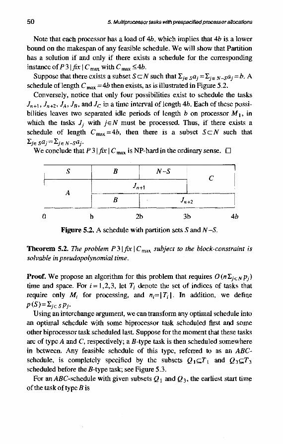
50 5. Multiprocessor tasks with prespecified processor allocations
Note that each processor has a load of 4b, which implies that 4b is a lower bound on the makespan of any feasible schedule. We will show that Partition has a solution if and only if there exists a schedule for the corresponding instance of P31fix I Cmax with Cmax ~4b.
Suppose that there exists a subset SeN such that Lje sai =Lje N-saj =b. A schedule oflength C max =4b then exists, as is illustrated in Figure 5.2.
Conversely, notice that only four possibilities exist to schedule the tasks ln+1, ln+2• JA, JB, and lc in a time interval of length 4b. Each of these possibilities leaves two separated idle periods of length b on processor M 1 , in which the tasks Ji with jEN must be processed. Thus, if there exists a schedule of length Cmax =4b, then there is a subset SeN such that
Lje saj =Lje N-saj. We conclude that P 31 fix I C max is NP-hard in the ordinary sense. D
s B I N-S i I c
ln+1 I A
I B I ln+2
0 b 2b 3b 4b
Figure 5.2. A schedule with partition sets S and N -S.
Theorem 5.2. The problem P31fix I Cmax subject to the block-constraint is solvable in pseudopolynomial time.
Proof. We propose an algorithm for this problem that requires O(nLjeNPi) time and space. For i = 1, 2, 3, let Ti denote the set of indices of tasks that require only Mi for processing, and ni= I Ti 1. In addition, we define p(S)=Lje SPj·
Using an interchange argument, we can transform any optimal schedule into an optimal schedule with some biprocessor task scheduled first and some other biprocessor task scheduled last. Suppose for the moment that these tasks are of type A and C, respectively; a B-type task is then scheduled somewhere in between. Any feasible schedule of this type, referred to as an ABC
schedule, is completely specified by the subsets Q 1 r;;;;.T 1 and Q 3 r;;;;.T 3
scheduled before theB-type task; see Figure 5.3. For an ABC-schedule with given subsets Q 1 and Q 3, the earliest start time
of the task of type B is

5.1. Makespan 51
Ql I E I Tl-Ql c T2
A Q3 I E I TrQ3
Figure 5.3. Structure of an ABC schedule.
The earliest start time of the task of type Cis then
Sc(Q 1 ,Q3)=max{SB(Q1 ,Q3)+pB +p(TI-Q 1), PA +p(T2) }.
The minimal length of such a schedule is therefore
0) C max(Q t.Q3) =max {Sc(Q 1 ,Q3)+ PC• SB(Q 1 ,Q3)+ PB + P (T rQ3)}.
Hence, the minimal length of an ABC-schedule is determined by p (Q 1) and p (Q 3 ). In other words, the length of an optimal ABC-schedule is equal to the minimum of C max (Q 1, Q 3) over all possible values of p (Q 1) and p (Q 3 ). Due to symmetry, we can transform any ABC-schedule into an CEA-schedule of the same length. The only other types of schedules of interest to us are therefore the EAC and ACE-schedules. Similar arguments show that the length of an optimal EAC-schedule is equal to the minimum of C max(Q 2,Q 3) over all possible values of p (Q 2) and p (Q 3), and that the length of an optimal ACEschedule is equal to the minimum of C max(Q 1 ,Q 2) over all possible values of p(Q1)andp(Q2).
Fori 1,2,3, we compute all possible values that p(Q;) can assume in 0 (n;p (T;)) time and space by a standard dynamic programming algorithm of the type also used for the knapsack and the subset-sum problems; see e.g. Martello and Toth [1990]. If these values are put in sorted lists, then all possible values that S B(Q t. Q 3) can assume are computed in 0 (p (Q 1 )+p (Q 3)) time and space. The minimum of C max (Q I, Q 3) over p (Q J) and p (Q 3) is then determined by evaluating expression (1) for each possible combination of p(Q I) andp (Q 3); this takes 0 (p(T 1)+p (T3)) time.
The lengths of the optimal EAC and ACE-schedules are determined similarly. The overall minimum then follows immediately, and an optimal schedule is determined by backtracing. Since n; -:;nand p(Ti)-:;J:,JeN Pi for each i, it takes 0 (nl:,JeNPJ) time and space to find an optimal schedule. D

52 5. Multiprocessor tasks with prespecified processor allocations
5.1.2. Strong NP-hardnessfor the genera/3-processor problem
Theorem 5.3. The problem P 31fix I C max is NP-hard in the strong sense.
Proof. The proof is based upon a reduction from the strongly NP-complete problem 3-Partition. It is similar to an earlier proof by Blazewicz, Dell'Olmo, Drozdowski, and Speranza [1992].
3-Partition Given an integer b and a multiset N = {a 1 , ... , a 3n} of 3n positive integers with b/4 < ai < b/2 and 'L}=t ai =nb, is there a partition of N into n mutually disjoint subsets N 1, .•. , Nn such that the elements in Ni add up to b, for j = 1, ... ,n?
number allocation processing time
n M2 &M3 (typeA) PA n Mt &M3 (typeB) PB n M 1 &M2 (type C) Pc
1 Mt PA+b n-1 Mt PA+b+pz
n Mt Py
n-1 M2 Pz n M2 PB+b+py
1 M3 Pc+Py n-1 I M3 Pc+py+Pz
Table 5.1. Separation tasks for P 31fix I C max.
Given an instance of 3-Partition, we construct the following instance of P 31fix I C max. There are 3n single-processor tasks Ji that correspond to the elements of 3-Partition; these tasks have to be executed by M 3 and their processing time is equal to ai, for j = 1, ... , 3n. In addition, there are 3n biprocessor separation tasks and 5n -1 single-processor separation tasks; there processing times and processing requirements are defined in Table 5.1. Here we define
PB=(n+1)b,
Py = (n + 1 )(b+p8 ),

5.1. Makespan 53
Pz =(n+l)(b+pn+Py),
Pc (n+l)(b+pn+Py+Pz),
PA (n+l)(b+ps+Py+Pz+pc).
Note that each processor has a processing load equal to "(=n(pA+Pn+Pc+Py+Pz+b)-pz, which implies that yis a lower bound on the makespan of any schedule. We will show that 3-Partition has an affirmative answer if and only if there exists a schedule with makes pan at most "( for the corresponding instance of P 3 I fix I C max.
If 3-Partition has an affirmative answer, then a schedule with makespan C max~ y exists, as is illustrated in Figure 5.4.
PA+b+pz
Pz
0
.... PA+b+pz I B I Py c c
.... Pz Ps+b+py
I Pc+Py+Pz A
b I B I Pc+Py
Figure 5.4. Structure for P31fix I Cmax: ABCAB · · · CABC.
Conversely, suppose that c;:ax ~y. Note that a schedule with makespan "( has no idle time. To avoid idle time at the start of a biprocessor task, both processors on which it has to be executed must have equal load. Hence, at the start of a task of type A, there exist a set T c N and integers Kt , K2 , K4 , Ks , 1C() , K7 E { 0, ... , n } K3 E { 0, ... , n -1 } , and K8 E { 0, 1 } , such that
(2) KtPA +K2Pc+K3Pz+K4(ps+b+py) = KsPA+lC(ips+K?(pc+Py+pz)+Kg(pc+py)+:EjeTPj·
Due to the choice of the processing times of the separation tasks, we draw the following conclusions:
- the sum TPj is a multiple of b, since PA, p8 ,pc.Py• andpz are multiples ofb,

54 5. Multiprocessor tasks with prespecified processor allocations
- ~je r Pi= 14b, since all other terms are multiples of (n +I )b, - Kt =Ks,sincepA>n(pc+Pz+Py+PB+b), - K2 =K7+Kg, sincepc>n(pz+Py+PB+b), - K3 =K7, sincepz>n(py+PB+b),
- 14 = K7+Kg, since Py>n (PB+b ), and - 14 =%,since ~jeTPj=14b.
It follows that
(3) Kt =Ks, K2=14 K6=K7+Kg, K3=K7, 14b=~jeTPj·
Analogous computations lead to similar relations that should hold at the start of a task of type Band C, respectively.
We will make extensive use of these relations in our analysis of the form that a schedule with makespan yshould have. Using an interchange argument, we see that there exists an optimal schedule in which a biprocessor task starts at time 0. We analyze the case that the first biprocessor task is of type B and that the next biprocessor task of another type is of type A; this case will be denoted as case BA. Hence, we have that no tasks of type A and C and at least one task of type B have been executed at the start of the first task of type A: K1 =K2 =K5 =0 and %~1. Expression (3), however, decrees that K2 =K5,
which yields a contradiction. Therefore, case BA cannot occur. A continued application of this argument shows that any schedule with makespan 'Y should have the form as displayed in Figure 5.4, or its mirror image. A schedule with this structure determines n separate periods of length b on processor M 3 , in which the remaining single-processor tasks have to be scheduled. These tasks correspond to the 3n elements of 3-Partition. We conclude that, if a schedule oflength yexists, then a solution to 3-Partition is obtained by taking the partition of N as defined by the schedule. We conclude that P 31fix I C max is NPhard in the strong sense. 0
5.1.3. Unit execution times, release dates, and precedence constraints
In this section, we show that the Pm lfix,pj=ll C max problem is solvable in polynomial time by providing an integer linear programming formulation with a fixed number of variables; a problem that allows such a formulation is solvable in polynomial time [H.W. Lenstra, Jr., 1983]. A similar approach is given by Blazewicz, Drabowski and Weglarz [ 1986].
Consider an arbitrary instance of the problem. There are at most M =2m -1 tasks of a different type; let these types be numbered 1, ... , M. We can denote the instance by a vector b=(b 1, ••• ,bM) in which component bi indicates the number of tasks of type j. A collection of tasks is called compatible if all these

5. 1. Makespan 55
tasks can be executed in parallel; hence, a compatible collection of tasks contains at most one task of each type. A compatible collection is denoted by a {0, 1 }-vector c of length M with cj = 1 if the collection contains a task of type j and zero otherwise. There are at most K =2M-I different compatible collections; this number is fixed, as M is fixed. Let the collections be numbered 1, ... , K; let the vectors indicating the collections be denoted by c 1 , ••• , c K.
The problem of finding a schedule of minimal length is then equivalent to the problem of finding a decomposition of this instance into a minimum number of compatible collections. Formally, we wish to minimize l:f=1xj subject to l:f=1 CjXj =b, Xj integer and nonnegative. As the number of variables in this integer linear programming formulation is fixed, we have proven the following theorem.
Theorem 5.4. The Pm lfix,pj=liCmax problem is solvable in polynomial time.
If the number of processors is specified as part of the problem type, implying that this number is no longer fixed, then things get worse from a complexity point of view. This is stated in the following theorem.
Theorem 5.5. The problem of deciding whether an instance of P lfix,pj = 11 Cmax has a schedule of length at most 3 is NP-hard in the strong sense.
Proof. The proof is based upon a reduction from the strongly NP-complete problem Graph 3-Colorability. A similar approach is used by Blazewicz, Lenstra, and Rinnooy Kan [1983].
Graph 3-Colorability Given a graph G=(V,E), does there exist a 3-coloring, that is, a function f :V -+{ 1,2,3} such that/ (u}:t:.f (v) whenever {u, v }E E?
Given an arbitrary instance G=(V,E) of Graph 3-Colorability, we construct the following instance of p I fix,p j= 11 c max. There are I v I tasks J 1' ... 'J I v I and I E I processors M 1 , ... 'M IE I . A task J u has to be processed by Me if u E e. We claim that there exists a 3-coloring forG if and only if there exists a schedule of length at most 3. Suppose that a 3-coloring of G exists. Since no two nodes u and v wit.lt the same color are adjacent, the corresponding tasks lu and lv require different processors. Hence, all tasks that correspond to

56 5. Multiprocessor tasks with prespecified processor allocations
identically colored nodes can be executed in parallel. This generates a schedule with length no more than 3. Conversely, in a schedule with length at most 3 we have that the nodes corresponding to tasks scheduled in time period t (t = 1,2,3) are independent; therefore, these nodes can be given the same color. This leads to a 3-coloril)g of G. Thus, P I fix ,pj = 11 C max is NP-hard in the strong sense. 0
Corollary S.l.For P lfix,pj = 11 Cmax• there exists no polynomial approximation algorithm with peiformance ratio smaller than 4/3, unless P = NP. 0
The introduction of precedence constraints leaves little hope of finding polynomial-time optimization algorithms. Even the two-processor problem with unit execution times and the simplest possible precedence relation structure, a collection of vertex-disjoint chains, is already NP-hard in the strong sense.
Theorem 5.6. The P21chain,fix,pj=liCmax problem is NP-hard in the strong sense.
Proof. The proof is based upon a reduction from 3-Partition and follows an approach of Blazewicz, Lenstra, and Rinnooy Kan [1983]. Given an arbitrary instance of 3-Partition, we construct the following instance of P 21 chain,fix,p j = 1 I C max. Each element a i corresponds to a chain Ki of 2a i tasks; the first part consists of ai tasks that have to be executed by M 1 and the second part also consists of a i tasks that have to be executed by M 2 • In addition, there is a chain L of 2nb tasks; groups of b tasks have to be alternately executed by M 2 and M 1 .
Suppose that there exists a partition of N into N 1, ••• , Nn that yields an affirmative answer to 3-Partition. A feasible schedule with makespan no more than 2nb is then obtained as follows. The chain Lis scheduled according to its requirements; the execution of L is completed at time 2nb. Now M 1 and M 2
are idle in the intervals [2(i-l)b, (2i-l)b] and [(2i-1)b, 2ib] (i=l, ... ,n), respectively. For each i E { 1, ... , n} it is now possible to schedule the three chains corresponding to the elements of Ni in [2(i-1)b, (2i-1)b] and [(2i-1)b, 2ib].
Conversely, suppose that there exists a feasible schedule with makespan no more than 2nb. It is clear that this schedule contains no idle time. Let N; be the index set of the chains Kj that are completed in the interval [ (2i -1 )b, 2ib]. It is impossible that 'f.jeN, aj > b due to the definition of N 1• The case 'f.jeN, aj<b

5.2. Sum of completion times 57
cannot occur either, since this would lead to idle time in [b, 2b ]. Therefore, we must have that L.jEN
1 ai =b. Through a repetition of this argument, it can be
easily proven that N 1, ••. , Nn constitutes a solution to 3-Partition. 0
The introduction of release dates has a similar inconvenient effect on the computational complexity.
Theorem 5.7. The P 21fix,ri I C max problem is NP-hard in the strong sense.
Proof. The proof is again based upon a reduction from 3-Partition. Given an arbitrary instance of 3-Partition, we construct the following instance of P 21 fix, ri I C max. For each element ai, we define a task Ji with Pi= ai and ri = 0 that has to be executed by M 1 • Furthermore, there are n tasks Ki with processing time band release date ri=(i-l)(b+£), for j= 1, ... ,n and E
sufficiently small; these tasks have to be executed by M 2. Finally, there are n -1 biprocessor tasks Li with processing time E and release date ri = jb +(i -1 )E, for 1=1, ... , n -1. It is easy to see that 3-Partition has an affirmative answer if and only if there exists a feasible schedule for P2lfix,rj I C max with C max :s;nb+(n-1)£. 0
Consider the case Pm lfix,ri,Pi = 11 C max where the number s of distinct release dates is fixed. Analogously to our analysis of Pm lfix,pi = 11 C max• we can transform any instance of Pm I fix ,ri,Pi = 11 C max into an integer linear programming problem with a fixed number of variables. We have proven the following theorem.
Theorem 5.8. The Pm lfix,rj,pj=ll C max problem with a fixed number of distinct release dates is solvable in polynomial time. 0
5 .2. Sum of completion times In this section, we investigate the computational complexity of our type of scheduling problems when we wish to minimize total completion time. Our main result is establishing NP-hardness in the ordinary sense for P21fix IL.Ci. The question whether this problem is solvable in pseudopolynomial time or NP-hard in the strong sense still has to be resolved. The weighted version, however, is NP-hard in the strong sense. We start with an easy observation. Given an instance, let the maximum processing time be denoted by
Pmax =maXjPj·

58 5. Multiprocessor tasks with prespecified processor allocations
Proposition 5.1. There is an optimal schedule for P I .fix I tCj in which the
tasks that require all processors for execution during Pmax time are scheduled
last, if they exist. D
Proof. Consider a schedule cr for P I .fix I tCj in which the task J that needs all processors for execution during time Pmax is not scheduled last. The interchange illustrated in Figure 5.5 generates a schedule cr* with tCj(cr*) $ tCj(cr) + p(B) fp(B)IPmaxlPmax $ tCj(cr), where p (B)= r,JjE BPj. D
B A B J
cr cr*
Figure 5.5. The interchange.
5.2.1. NP-hardness for the 2-processor problem.
Theorem 5.9. The P2l.fix I tCj problem is NP-hard in the ordinary sense.
Proof. Our proof is based upon a reduction from the NP-complete problem Even-Odd Partition.
Even-Odd Partition Given a multi set of 2n positive integers A = {a 1 , ••• , a 2n } such that a; < a; +I
(i = 1, ... , 2n -1), is there a partition of N into two disjoint subsets A 1 and A 2 with equal sum b = t~1 aJ2 and such that A 1 contains exactly one of {a2i-l ,a2;}, for each i = 1, ... , n?
Given an instance of Even-Odd Partition, define p = (n 2 + 1 )b, q=n 2(n 2+1)(n+l)p, and r=t}=1(n+j-1)(a 2j-t+a2j)+n 2(n+l)b. We construct the following instance of P 21.fix I tCj. Each element a j corresponds to a partition task Jj with processing time Pi =nb+aj that has to be executed by M 1• In addition, we define n 2+3 extra tasks. There are n 2 identical tasks Q;
( i = 1, ... , n 2) with processing time 2p (n + 1) that have to be executed by M 2, a task K with processing time p that has to be executed by M 2, a biprocessor task L with processing time p, and a task P with processing time 2p (n + 1) that has to be executed by M 1• We will show that Even-Odd Partition is answered affirmatively if and only if there exists a schedule for the corresponding instance of P 21.fix I tCj with total completion time no more than the threshold

5.2. Sum of completion times 59
y =(2n 2+4n+8)p+q+r.
Suppose that there exist subsets A 1 and A 2 that lead to an affirmative answer to Even-Odd Partition. Then there exists a schedule cr* with total completion time no more than y, as is illustrated in Figure 5.6: the completion times of the extra tasks add up to (2n 2+2n+8)p+q, the sum of the completion times of the partition tasks is equal to 2np +r.
A1 Az I p I L
K Q1
•
·······
0 p 2p 3p (2n+4)p
Figure 5.6. The schedule cr* with partition sets A 1 and A 2 .
Conversely, suppose that there exists a schedule cr with total completion time no more than y. We first show that the extra tasks in cr must be scheduled according to the pattern of Figure 5.6.
A straightforward computation shows that task P and the Q-tasks must be completed after all other tasks in cr. Suppose that task L precedes task K, and that m partition tasks are completed before L starts. Note that m ~ n; otherwise, task K could be scheduled parallel to the m partition tasks, without increasing the completion time of any other job. If we compare this schedule with cr*, then task L turns out to be the only task with smaller completion time; this gain is more than offset by the increase of completion time of task K. Hence, in order to satisfy the threshold, the extra jobs must be scheduled according to the pattern of Figure 5.6.
We now show that, if I:.Ci ( cr) ~ y, then the partition tasks must constitute an affirmative answer to Even-Odd Partition. First, suppose that the partition tasks before L in cr have total processing time smaller than p, implying that at most n partition tasks are scheduled before L. Then the total completion time of the partition jobs amounts to at least r+2np, the total completion time of the Q-tasks, task K, and task Lis equal to the total completion time of these tasks in cr*, and the completion time of task Pis greaterthan 3p+(2n+2)p, implying that the threshold is exceeded. Hence, the total processing time of the partition tasks before task L amounts to at least p.
Now suppose that m partition tasks with total processing time p+x precede task L. Comparing cr with cr* shows that the total completion time of the extra jobs in cr isx(n 2+1) greater and that the difference in total completion time of the partition tasks is no more than 2p (n -m )+x (2n -m) in favor of cr. If m = n,

60 5. Multiprocessor tasks with prespecified processor allocations
then the difference in total completion time between cr* and a is at least equal to x (n 2+ 1)-xn in favor of a*; x > 0 then clearly implies that the threshold will be exceeded. In case m > n, we wish to show that x(n 2+1) > 2p(n-m)+x(2n-m), which boils down to showing that x(n 2+1-2n+m) > 2p(n-m). As the left-hand-side of the inequality is positive and the right-hand-side negative, we have that the case m > n leads to an excess of the threshold. Hence, exactly n partition tasks with total processing time equal top must precede task Lin cr. The total completion time of the partition tasks is equal to 2np + n (p [l ]1 +p [1]2) + · · · + (p [n Jl +p [n 12), where p [i] 1
and p [il2 denote the processing time of the [i ]th partition task before L and after L, respectively. It is easy to see that the threshold can only be met if {p £i]1 ,p [il2} = {P2H ,p2;}, for i = 1, ... , n. Define A I and A 2 as the set of partition tasks before L and after L in a, respectively. As the total processing time of the tasks in A 1 amounts to n 2b+:EA
1ai =p =(n 2+1)b, we have that the
corresponding subset of partition elements has sum equal to b. Furthermore, A I contains exactly one element from every pair {a 2i -I , a 2i } ; hence, the subsets A 1 andA 2 lead an affirmative answer to Even-Odd Partition. D
Theorem 5.10. The P 21fix I:EwiCi problem is NP-hard in the strong sense.
Proof. The proof is based upon a reduction from 3-Partition. Given an arbitrary instance of 3-Partition, we construct the following instance of P21fix l:EwiCi. Each elementai corresponds to a taskli with processing time ai and unit weight that has to be executed by M I· In addition, there are n tasks Ki with processing time b and weight 2(j +a-1 )~ that have to be executed by M 2 , and nL biprocessor tasks Li with processing time band weight (2j-1)~, where a= 3n (2n -1 ), ~ = ab, and nL = a+n -1.
Suppose that there exists a partition of N into N I, ... , Nn that yields an affirmative answer to 3-Partition. A feasible schedule with sum of weighted completion times no more than
y = ~.:Ek=1 wk(2(n -k)+1)b+.:Ef=I Wz(2n +a-l)b+:E7~+1 wz(2n -2(1-a))b
is then obtained by scheduling the tasks as illustrated in Figure 5. 7. Conversely, suppose that there exists a schedule a with sum of weighted
completion times no more than y. Straightforward computations show that the K-tasks and the L-tasks have to be scheduled as indicated in Figure 5.7 and that the tasks Ji have to be scheduled in the time slots parallel to the K-tasks. Let Ni denote the set of ]-tasks that are scheduled parallel to Ki; the sets N 1, ••• , Nn constitute a solution to 3-Partition. D

5.2. Sum of completion times 61
Nn Nn-1
Kn LnL
Kn-1 Lnc1
N1 La. La.-1
K1 •••••••[] 0 b 2b 2nb
Figure 5.7. A schedule for P 21fix I I.wiCi with I.wiCi ~y.
5.2.2. Strong NP-hardnessfor the general3-processor problem
Theorem 5.11. The P 31fix I I.Cj problem is NP-hard in the strong sense.
Proof. The proof is based upon a reduction from the decision version of the P 31 fix I C max problem, which was shown to be NP-complete in Section 2.2. The decision version of P 3 I fix I C max is defined as the following question: given an instance of P 31fix I C max and a threshold b, does there exist a schedule cr with makespan no more than b?
Given an arbitrary instance of P 31 fix I C max and a threshold b, we construct the decision instance of P 3 I fix I I.Cj by adding nb + 1 identical triprocessor tasks Ki with processing time p max. The corresponding threshold is equal to y =nb+I.;:~T1 (b+kPmax).
Application of Proposition 5.1 shows that there is an optimal schedule with the K-tasks executed last. The number of K-tasks is such that the threshold will be exceeded if the first K-task starts later than b. Hence, the decision variant of P 31fix I I.Cj has an affirmative answer if and only if the decision variant of P 31 fix I C max has an affirmative answer.
Note that, the number of tasks needed in our reduction is pseudopolynomially bounded. We conclude that P 31fix I I.Cj is NP-hard in the strong sense. D
5.2.3. Unit execution times and precedence constraints
In this section, we address the complexity of minimizing total completion time in case of unit processing times. We show that P I fix ,pi= 11 I.Cj is NPhard in the strong sense; the complexity of this problem with a fixed number of processors is still open.
Theorem 5.12. The P I fix ,pi= 11 I.Cj problem is NP-hard in the strong
sense.

62 5. Multiprocessor tasks with prespecified processor allocations
Proof. The proof of this theorem is based upon a reduction from PI fix ,pi= 11 Cmax; it proceeds along the same lines as the proof of the previous theorem. Given an instance of P !fix ,pi= 11 C max• we add w tasks that require all processors for execution; application of Proposition 5.1 shows that these tasks can be assumed to be executed after all other tasks. By choosing w suitably large, we obtain the situation that the threshold of P I fix ·Pi= 11 r.ci is exceeded if and only if the threshold of P I fix ,pi II C max is exceeded. As the decision variant of P !fix ,pi= 11 C max is NP-complete in the strong sense and as w is polynomially bounded, we conclude that P !fix ,pi= 11 r.ci is NPhard in the strong sense.
As could be expected, the addition of precedence constraints does not have a positive effect on the computational complexity. We show that even the mildest non-trivial problem of this type, with two processors and chain-type precedence constraints, is NP-hard in the strong sense.
Theorem 5.13. The P 21 chain,fix,prl! r.cj problem is NP-hard in the strong sense.
Proof. The proof is based upon the same reduction as used in the proof of Theorem 5.6, only the threshold differs. As the number of tasks is equal to 2nb, and as each task has unit processing time, an obvious lower bound on the total completion time is equal to y = 2nb (2nb + 1 ); this bound can only be attained by a schedule without idle time in which both processors execute nb tasks. Hence, there exists a schedule with total completion time no more than y if and only if there exists a schedule with makespan no more than b. We conclude that P 21 chain,fix,pi=ll r.cj is NP-hard in the strong sense. D

6. Chains of length 1, or the two-stage flow shop

64 6. Chains of length 1, or the two-stage flow shop
In the previous chapter we dealt with prespecified processor allocations. In general, an instance may consist of tasks that still have to be allocated as well as tasks with a prespecified allocation. An example of such a situation occurs in a two-stage pipeline, where the first stage consists of two independent identical processors and the second stage is built up of a single processor. This model is described more precisely as follows.
A set of 2n tasks has to be processed by three processors. Each of the first n tasks Jj is to be executed by one of the first two processors M 1 and M 2 . The remaining n tasks Kj belong to a single family, which is entirely executed by the third processor M 3 • The tasks are related through a precedence relation that consists of a collection of chains of length l; Ji precedes Kj for j = 1, ... , n. Preemption of tasks is allowed, which means that the processing of a task may be interrupted and resumed at the same time on a different processor or at a different time on the same or a different processor. However, each task can be active on only one processor at a time. The objective is to minimize makespan.
The problem described above belongs to the class P31chain,Jam,set,pmtn ICmax· It is a special case of the class of two-stage flow shop scheduling problem, where each stage is executed by a number of processors. Related nonpreemptive problem types have been addressed by several researchers. Salvador [ 1970] investigates the problem of finding a permutation schedule of minimal length in an m-stage no-wait flow shop environment with an arbitrary number of parallel processors in every stage. Buteo and Shen [1973] propose two heuristics for the two-stage problem with an arbitrary number of parallel processors in each stage and analyze their worst-case behavior, whereas Arthanri [1974] designs a branch-and-bound algorithm for the same problem.
We consider the problem from a complexity point of view. The problem can be seen as an immediate generalization of the preemptive version of the classical two-stage flow shop problem, which has a single processor at each stage, and the problem of minimizing makespan on two parallel processors allowing for preemption, p 21pmtn I c max. For the classical two-stage flow shop problem, Johnson [1954] derived an O(nlogn) time algorithm; it also constructs optimal schedules for the preemptive version, since preemption does not help. Mc-Naughton's [1959] wrap-around rule solves P lpmtn I Cmax in O(n) time. However P 211 C max is NP-hard, so that the nonpreemptive problem P 31 chain,fam,set I C max is NP-hard as well. In this chapter, we show that the preemptive problem described above is NP-hard in the strong sense.
The organization of this brief chapter is as follows. We first show that the

6. 1. Ordinary NP-hardness 65
problem P 31 chain,fam,set,pmtn I C max is NP-hard in the ordinary sense in Section 6.1. In Section 6.2, we use the basic idea of that proof to obtain the more general result that the problem is NP-hard in the strong sense.
6.1. Ordinary NP-hardness In this section, we show ordinary NP-hardness of the problem P 31 chain,fam,set,pmtn I C max by a reduction from Partition. This reduction will provide the insight needed to establish NP-hardness in the strong sense.
Partition Given a multiset N = {a 1 , ..• , an} of n integers, is it possible to partition N into two disjoint subsets that have equal sum b='LjENajl2?
Given an instance of Partition, construct the following instance of P 31 chain,fam,set,pmtn I C max with a precedence relation consisting of chains of length 1. For each j e N we define two partition tasks Jj and Kj; Ji has processing time aai and Ki has processing time aj, where a> 1. In addition, we define eight separation tasks, which have to create time slots of equal length for the execution of the partition tasks. The processing times of the separation tasks are given in Table 6.1. The precedence constraints are such that lr-?Kj, for j = 1, ... , n +4. The tasks of type J can be performed by processors M 1 and M 2 ; the tasks of type K have to be performed by M 3. Note that 2( ab +b) is a lower bound on the makes pan and that a schedule with C max = 2( ab +b) contains no processor idle time.
j n+1 n+2 n+3 n+4
Jj 0 ab+b ab+2b b
Ki ab ab 0 0
Table 6.1. Processing times of the separation tasks.
SupposeS is a subset of N with sum equal to b. We construct the following schedule oflength 2(ab+b). The processing ofthe set of J-tasks corresponding to the elements of S starts at time 0 on M 1 • These tasks are executed consecutively and their execution takes ab time. The processing of the set of Ktasks corresponding to S starts at time ab; it is preceded by the execution of task Kn+l· Task ln+2 starts at time 0 and is executed without interruption by M 2 • Its successor Kn+2 is processed without any delay. The execution of the set of remaining partition tasks of type J starts at time ab + b and the execution

66 6. Chains oflength 1, or the two-stage flow shop
of the set of their successors starts at 2ah+b following Kn+Z· Finally, the remaining two separation tasks are added to complete the schedule; for an illustration see Figure 6.1.
0 ah ah+b 2ab+b 2(ah+b)
Figure 6.1. A schedule with partition sets S and N- S.
Conversely, suppose that a schedule cr exists with makespan 2(ah+b). Without loss of generality, we may assume that the K-type tasks are executed without preemption in order of completion time of their predecessors. Since cr contains no processor idle time and In+ I is the only task of type J with processing time equal to 0, task Kn+l completes at time ah. For similar reasons, tasks 1n+3 and 1n+4 complete at time 2(ab+b). Let ln+Z complete at time ah +b+Ll, with Ll ~ 0. Processor M 3 should perform partition tasks of type K from time ah to time ah +b +Ll. Their predecessors have to be performed by M 1 and M 2 before ln+Z and 1n+3 start; the execution of these partition tasks takes at least time a(b+Ll). The amount of time available is ah+Ll. From a(b+Ll):S;ab+Ll and a> 1, it follows that Ll=O and the total processing time of the partition tasks of type J that are processed before 1n+3 is started is equal to ah. Hence, such a schedule cr gives a certificate of the affirmative answer to Partition.
By now, we have proven the following theorem.
Theorem 6.1. The problem P 31 chain,fam,set,pmtn I C max is NP-hard, even with a precedence relation consisting of a collection of chains of length 1.
6.2. Strong NP-hardness In this section, the above described problem, P 31 chain,fam,set,pmtn I C max,
is shown to be NP-hard in the strong sense. We use the 3-Partition problem for our reduction.

6.2. Strong NP-hardness 67
3-Partition Given an integer b and a multiset N = {a 1 , ... , a 3n } of 3n positive integers with b/4 < aj < b/2 and :r.J~ 1 aj =nb, is there a partition of N into n mutually disjoint subsets N 1, ••• , Nn such that the elements in Nj add up to b, for j 1, ... ,n?
j 6n+1 6n+2 6n+3 ?n 7n+l 7n+2
Jj 0 ah+b ah+2b ab+2b ah+2b b Kj ah ah ah ah 0 0
Table 6.2. Processing times of the separation tasks.
Given an instance of 3-partition, we construct the following instance of P 31 chain,fam,set,pmtn I C max with a precedence relation consisting of chains of length 1. As in Section 6.1, for each j e N we define two partition tasks Jj and Kj; Jj has processing time aa j and Kj has processing time a j, where a>l. In addition, we define 2(n+2) separation tasks; their processing times are given in Table 6.2. These tasks have to create time slots. The precedence constraints are such that lr~Kj, for j = 1, ... , 7n+2. The tasks of type J can be performed by processors M 1 and M 2 ; the tasks of type K have to be performed by M 3• Note that n ( ah +b) is a lower bound on the makespan and that a schedule with C max = n ( ah +b) contains no processor idle time.
Proposition 6.l.If 3-partition has an affirmative answer, then the instance defined above has a schedule of length n ( ah +b).
Proof. Let N t. ... , N n constitute a yes-answer for the 3-Partition instance. Consider the schedule given in Figure 6.2. Straightforward computations show that the makespan of this schedule is equal ton ( ah +b). 0
In order to show the converse implication, that is, that 3-Partition has an affirmative answer if the instance P 31 chain,fam,set,pmtn I C max has a schedule of length n ( ah +b), we need the following propositions. The proofs follow from the same arguments as used in the proof of Theorem 6.1 and are therefore omitted.
Proposition 6.2. There exists an optimal schedule such that Jj and Kj are completed no later than Jj+l and Kj+l> respectively, for j =6n+1, ... , 7n+2.

68 6. Chains of length 1, or the two-stage flow shop
·I K7n-l
0 (ab+b) 2(ab+b) n(ab+b)
Figure 6.2. A schedule with partition sets N 1, ••• , Nn.
Proposition 6.3. A schedule of length n ( fJ.b +b) satisfies the following properties: - it contains no processor idle time, - Jj completes at time U-6n-l)(fJ.b +b ),for j =6n+l, ... , 7n+l, - Kj starts immediately after Jj is completed, for j =6n+1, ... , 7n+2. D
Proposition 6.4. Let cr be an optimal schedule of length n(fJ.b +b) that satisfies Proposition 6.2. Then cr certifies that the 3-Partition instance is a yes-instance. D
Since the above reduction requires polynomial time, we have now proven the following theorem.
Theorem 6.2. The problem P 31 chain,fam,set,pmtn I C max is NP-hard in the strong sense, even for a precedence relation consisting of a set of chains of length 1. D
Corollary 6.1. The problem P31chain,fam,set I C max is NP-hard in the strong sense, even for a precedence relation consisting of a set of chains of length 1. 0

7. Tosca: methodology

70 7. Tasca: methodology
From the analyses of the previous chapters, we may conclude that it is unlikely that fast algorithms exist that solve the scheduling problem in its most general form to optimality. One is confined to take an approximative approach. In the remaining chapters of this thesis we describe such an approach. We introduce Tosca, our tunable off-line scheduling algorithm, which produces approximate answers to instances of a special case of the problem type P lprec,com,fam,set I C max described in Section 7.1. Tosca has been developed as a tool to support the scheduling of parallel programs on distributed memory architectures.
Tosca is an algorithm that tries to find a reasonable solution in a reasonable amount of time by bounded enumeration, as will be described in Section 7 .2. Only a part of the solution space is taken into consideration, and the user is given the facility to determine the size of this part.
Tosca is tunable in the sense that it enables the user to control the speed of the solution method and the quality of the schedules produced. First of all, the size of the part of the solution space considered influences both quality and speed. Moreover, the user has to define priority rules for the selection of tasks and processors, a lower bound rule for truncating the enumeration process, as well as an evaluation rule for the evaluation of partial schedules. A number of predefined rules are incorporated in Tosca, but the user has the opportunity to· define new rules, as described in Section 7 .3.
Lower bounds on the makespan of an optimal schedule also provide the user with a measure of the quality of the schedules produced by Tosca. The lower bounds are based on the total amount of work that has to be done and on the structure of the precedence relation. They are described in Section 7 .4.
7 .1. The problem type A collection of m identical parallel processors Mi (i =1, ... , m) has to process a set of n tasks Ji (j=l, ... ,n). The task set is partitioned into a number of families. Each task belongs to a single family. Tasks that belong to the same family F have to be executed by the same processors. Each task in F can be performed by any collection of processors of a given family-dependent size sp, unless F has a nonempty collection of processors specified as part of the problem instance. In the latter case, each task in F is fixed to this prespecified collection of processors. The processing of task Ji takes pi time. Let Fi denote the family Ji belongs to.
With each task Ji two data sets li and Oi are associated, representing the data that this task requires and delivers, respectively. The data dependency between two tasks Ji and Jk is defined as follows. The tasks are independent if

7.2. The solution method 71
0/"'lh=Oknli=0. If 0/1h::t0 and Oknlj=0, then we write lr~h and require that Jj has been completed before Jk can start. Conversely, if Oknlj * 0 and 0/1/k = 0, then we write Jk~Jj and require that h has been completed before Jj can start. The case that 0 in/ k ::t 0 and Oknlj ::t 0 should not occur, since it would represent a loop in the parallel program. Thus, the data dependencies impose a precedence relation on the task set. It is denoted by an acyclic directed graph G with vertex set { 1, ... , n } and an arc U, k)
whenever Ji~h. Let Pi= {h lh~lj} and Qj= {h llj~Jd denote the sets of predecessors and successors of Jj, respectively.
Communication delays due to these data dependencies are modelled as follows; see also Section 2.3. Let D be the set containing all information: D =u}=t oj. Each data item aE D has a given integer weight Wa, and the weight of a data set U c D is defined by w ( U ) = I:aE u w a. The communication cost function c specifies the time needed to transmit a data set of a given weight from one processor to another. It is assumed to be of the form c (x) = c 1 +c zl x/c 31 +c l x/c 512 and is therefore defined by the integral constants c 1 , ... , c 5 . lnterprocessor communication occurs when a task h needs information from a predecessor Jj and makes use of at least one processor that is not used by Jj. Let Mi be such a processor and let P(k,i) denote the set of tasks scheduled on Mi before and including Jk· Prior to the execution of h, the data set U(i,j,k)=u1E Q/•P(k,i)(0/1/1) has to be transmitted to Mi, since not only h but also each successor of Jj that precedes h on Mi requires its own data set. The time gap in between the completion of Jj (at time Cj) and the start of Jk (at time Sk) has to allow for the transmission of U (i,j,k). The communication time is given by c (w (U (i,j,k))). For feasibility it is required that Sk~Ci ~c (w (U(i,j,k))).
A schedule is an allocation of each task Jj to a time interval of length Pi on sy processors such that no two of these time intervals on the same processor
J
overlap. A schedule is feasible if it meets the requirements concerning the pro-cessor environment and the task characteristics as described above. A feasible schedule is active if no task can be moved forward in time without delaying some other task or violating the constraints. Tosca aims to minimize the length of a schedule.
7 .2. The solution method An active schedule can be constructed by iteratively selecting the next task to schedule, allocating a collection of processors to it, and starting it as early as possible. We can visualize the various possible choices by an enumeration tree, as shown in Figure 7 .1. In Figure 7.1 a we present an instance consisting

72 7. T osca: methodology
of two processors, four tasks, and four families. The enumeration tree for this instance is given in Figure 7.lb, where the root represents the empty schedule, each 0-node represents the selection of a task, and each D-node represents the allocation of a task to a collection of processors. Hence, each D-node corresponds to a partial schedule of the tasks selected so far, and the leaves of the enumeration tree correspond to all complete schedules.
The process of bounded enumeration consists of n stages. At each stage an available task and a collection of processors for that task is selected. A task is said to be available if all of its predecessors have been scheduled. In order to select a task and a processor collection, Tosca generates a subtree of the enumeration tree, as shown by the double boxes and circles in Figure 7.1b. In total, n subtrees have to be generated until a complete schedule has been constructed.
The subtree is determined by three parameters d, t, u, two priority rules, and a lower bounding procedure. The parameter d defines the depth of the subtree. At each of the d levels, Tosca applies the first priority rule to select t of the available tasks and, for each chosen task, Tosca applies the second priority rule to select u of the processor collections that can execute the task. For each partial schedule that is generated, Tosca computes a lower bound on the optimal makespan of schedules that are extensions of the partial schedule. If this lower bound exceeds a given upper bound, then the branch determined by the partial schedule is eliminated and will not be examined further. The parameters d, t, u, and the lower bounding procedure determine the size of the subtree that is rooted at the current partial schedule.
The leaves of the subtree are partial schedules, which are evaluated according to an evaluation rule. Each task-collection pair chosen at the first level determines a branch of the subtree; each branch contains a number of leaves, each with its own value. A task-collection pair that leads to a leaf of minimal value is chosen and a new partial schedule is constructed, as shown by the bold boxes in Figure 7.1 b. A new stage has been reached.
As said before, Tosca is tunable in the sense that it allows the user to control the speed of the solution method and the quality of the schedules produced. First, by adjusting the three parameters d, t, and u, the user influences the size of the partial tree that is computed and chooses from a range of possibilities in between list scheduling and complete enumeration. Second, the user has to define two priority rules: one for selecting a task and another for selecting a collection of processors. And finally, the user has to specify a lower bound rule for the bounding procedure and an evaluation rule for partial schedules.

7.2. The solution method
m=2 n=4 s 1 =2, s 2 = 1, s 3 =2, s4 =2
Figure 7.1a. An instance of P lprec,com,fam,set I Cmax·
Figure 7.lb. Enumeration tree. Double boxes and circles indicate a subtree for d = 3, t = 2, and u = 1. The bold circle and the bold box adjacent to it indicate a chosen task and processor allocation; the other bold box is the 'best' leaf in the partial tree. The current partial schedule is the empty schedule.
73
Given a problem,·Tosca starts with priority scheduling. An evaluation rule and two priority rules are chosen and the parameters d, t and u are set to 1.

74 7. Tasca: methodology
Repeatedly a task of high priority among the available tasks is selected and allocated to a processor collection of high priority. The makespan of the resulting schedule is the initial upper bound on the optimal makespan.
Lower bounds on the makespan of an optimal schedule are computed at the start of Tosca. These lower bounds provide the user with a measure of the quality of the schedules produced by Tosca. A description of these lower bounds is given in Section 7.4.
attribute name value forJj
static number of processors m m number of tasks n n processing time pj Pi
size sF SFi
cardinality of the indata set #in IIi I cardinality of the outdata set #out !Oil
weight of the in data set win w(lj) weight of the outdata set wout w(Oj) number of predecessors #pre IPil
number of successors #sue IQil list index list j
longest preceding path head longest succeeding path tail
Papadimitriou-Y annakakis PapYan dynamic first in first out fifo
minimal starting time start
Table 7.1. Task attributes.
7.3. Priority rules, evaluation rule, and lower bound rule A priority rule for the selection of tasks depends on one or more task attributes. A task attribute is static if it can be computed on the basis of the data that defines a problem instance. It is dynamic if schedule information is required for its computation. The various task attributes are listed in Table 7 .1.
Given a task Ji, the attribute head is the length of a longest path from a source node to Ji and the attribute tail is the length of a longest path from Ji to a terminal node. The attribute Pap Van is a lower bound on the starting time of Ji. It is computed similarly to head, but communication delays are taken into account; cf. Section 7.4. The attribute fifo assigns to a task its rank with

7.3. Priority rules, evaluation rule, and lower bound rule 75
respect to the point in time at which it becomes available. Given a partial schedule, the earliest starting time can be computed for any available task; start assigns this value to each available task.
The predefined priority rules that are incorporated in Tosca determine an order in which the tasks are considered with respect to a given attribute. The predefined priority rules are min-sF, max-sF, max-#suc, min-list, maxhead, min-tail, min-PapYan, min-fifo, and min-start. If the tasks are considered in order of nondecreasing attribute value, then the prefix min is used in the name of the priority rule. The prefix max is used if the tasks are considered in order of nonincreasing attribute value. The predefined priority rule min-sF, for example, gives high priority to the tasks of small size, whereas the priority rule max-sF gives high priority to the tasks oflarge size.
priority rule for tasks: lexico(expression, ... , expression) expression
expression:
tenn:
expression+ term expression- term max {expression, term} min (expression, term} term
term I primary term *primary primary
primary: number -primary attribute ( expression )
Figure 7.2. Grammar for priority rules.
The user is given the facility to build a priority rule for the selection of tasks based upon the task attributes. This may involve the construction of new attributes on the basis of old ones. The grammar for a user defined priority rule that is accepted by Tosca is given in Figure 7 .2. In words, a user defined priority rule consists of a single expression or the operator lexico applied to several expressions. The basic units of an expression are numbers, task attributes, and

76 7. T osca: methodology
the operators *,/,max, min,+, and- (both unary and binary). An expression assigns a value to each task, which is then a new, user defined, task attribute. The tasks are considered in order of nondecreasing value with respect to each expression. Thus, the predefined priority rule max-tail leads to the same outcome as the user defined priority rule that consists of the expression -tail.
A priority rule for the selection of collections of processors depends on the static and dynamic processor attributes given in Table 7 .2. As said in Section 7 .2, Tosca applies a task priority rule to select a number of available tasks and, for each chosen task Jj, Tosca applies a processor priority rule to select a number of the processor collections that can execute the task. The attributes #pre and data depend on the available task (Jj) under consideration. The attribute data determines the point in time that Ii can be available on Mi, for i=l, ... ,m. The predefined priority rules are all based on dynamic attributes; they are min-fut, min-load, max-#pre, and min-data. Again, the user is enabled to construct a new priority rule. The grammar that is accepted by Tosca is the same as the grammar for user defined task-priority rules given in Figure7.2.
attribute name valueforMi
static number of processors m m number of tasks n n
dynamic future fut maxJjonMiCi load load LJionM,Pj
number of predecessors #pre IPin{JkllkonMd I data available data
Table 7.2. Processor attributes.
Static attributes used in a priority rule are computed before the (bounded) generation of the enumeration tree. Dynamic attributes are computed during the generation of the enumeration tree.
An evaluation rule assigns values to partial schedules. The following evaluation rules are available:
- makespan: the length of the partial schedule is computed; - completion plus tail: for each taskJi, the length of a longest path starting at
Ji is added to its completion time and the maximum of these values is taken; - partial plus Pap Van: an adaptation of an algorithm of Papadimitriou and
Yannakakis [1990] applied to the partial schedule yields lower bounds on

7.4. Lower bounds on the makespan 77
the completion times of the tasks and the maximum of these values is used; see also Section 7 .4.
A lower bound rule is used to eliminate branches of the enumeration tree that will surely not lead to improvements. The user is enabled to chose from the following two rules:
makespan: the length of the partial schedule is used as lower bound; - partial plus Pap Van: an adaptation of an algorithm of Papadimitriou and
Y annakakis [ 1990] applied to the partial schedule yields a lower bound on the makespan.
7.4. Lower bounds on the makespan Tosca computes three lower bounds on the makes pan of an optimal schedule. For ease of use, we define c(j,k)=c(w(O/Ift)) and Sj as the (family dependent) number of processors Jj requires for execution. The lower bound work load is defined as "L}=I (pjsj)lm. The lower bound longest path is the length of a longest path with respect to the precedence relation; if J 1 ---7 · • • ---711 is a path, then the length of this path is "L1.,jgpj+Lt::;;j::;;l-1,sj<s
1+
1c(j,j+l). The
third lower bound is based on an algorithm of Papadimitriou and Y annakakis [ 1990]. A modification of this algorithm leads to a lower bound that dominates longest path. It is described below.
First, the procedure computes a lower bound bj on the starting time of each task Jj. Zero lower bounds are assigned to tasks without predecessors. For any task Jk other than such a source task, consider its predecessors. For each predecessor Jj of Jk, define .{j as .{j =bj+pj+c (j,k). In any schedule, a communication delay occurs in between any (predecessor, successor) pair of tasks Jj,Jk satisfying sj< sk. Definebl as bl=max {.{j ljePk andsj< sk }.
Sort the predecessor subset { Jj I JjE P k and s j ;:::: sk } in decreasing order of J, that is, .{j,;:::: · · · ;:::_{jq. Given an integer y satisfying_{j,;:::y;:::_{j,+,, consider the following single-processor scheduling problem with release dates on i tasks (L 1, ... , Li). The release date of a task is the point in time at which it becomes available for processing. Task L1 corresponds to task Jj
1, that is, it has process
ing time p1 = Pj1
and release date r1 = b j,. Let C max ( y) denote the minimal makespan of this single-processor scheduling problem. Define bt as the least integer y such thaty;::: Cmax(y).
The lower bound bk on the starting time of Jk is now defined as the maximumofbl andbt. ThelowerboundPapYanisgiven bymaxj { bj+Pj }.
Given a feasible schedule, let Jk be scheduled at time Sk and let all of its predecessors be scheduled at or after their lower bounds. Clearly, for

78 7. Tasca: methodology
feasibility it is required that sk;::: b}. Each predecessor Jj that satisfies Sj;::: Sk and .{j>Sh has to be executed by (at least) the same processors that execute h to prevent communication delays that would occur otherwise. Therefore, the corresponding single-processor scheduling problem mentioned above has makespan C~ax 5.Sk. Since b~ is the least integer satisfying such constraints, we may conclude that bk 5, Sk. It follows that PapYan is indeed a lower bound on the schedule length.
Due to the analyses of Papadimitriou and Y annakakis [ 1990] and Colin and Chretienne [1991], one may expect the lower bound PapYan to be tighter for problem instances with a relatively large number of processors, and for problems where the communication delays are small with respect to the processing times.

8. Tasca: implementation

80 8. Tosca: implementation
The methodology of Tosca as described in the previous chapter has been implemented using the computer language GNU C++. The overall organization of Tosca and the results of experiments with Tosca are reported in this chapter. Together, Sections 7.3, 8.1, and 8.2 form a manual for the use of Tosca.
At the start of Tosca, a problem instance is read from a file that is specified by the user. The user can also specify a file to save Tosca's results, such as a schedule and a parameter setting with a corresponding makespan. The input and output specification is given in Section 8.1.
We developed a user interface that supports the presentation of problem instances and solutions. The man-machine interaction is menu driven, in such a way that at any moment all feasible commands are visible. The user interface and the functional properties ofTosca are described in Section 8.2.
Tosca has been tested on four classes of problem instances. The first class contains instances where the precedence relation has a layered structure, the instances of the second class have a series parallel precedence relation, and the third class consists of instances with arbitrary precedence relations. With respect to the fourth class, two precedence relations from practice were at our disposal; we generated data sets, processing times, and task sizes to obtain new instances. The four problem generators are given in Section 8.3.
In Section 8.4 the results of the tests are tabulated and analyzed.
name m n W~t···•WIDI
PI ·I · f/,1 lJ ' .•• 'lJ
1 jO,j OJ, .•. ,OJ FI
Pn ·I .j/, I ln' •.. 'l n
1 JO.I Om ... ,On Fn
SJ MI •... ,M'i'
sf M}, ... ,Mf C1 c2 C3 c4 cs
Table 8.1. Format of an input file.
8.1. Input and output specification A problem instance is read from a file that is provided by the user. The instance has to belong to the problem class described in Section 7.1. The format of the input file is specified in more detail in Table 8.1. First of all, the problem name, the number of processors and the number of tasks are given.

8. 1. Input and output specification 81
Next the weights of the individual data items are specified. Tosca then requires the following data for each task Jj: processing time, the data set Ij that is required for execution, the data set Oj that is delivered after completion of the task, and the index Fj of the family Jj belongs to. Following the task characteristics Tosca requires for each family the number of processors each of its tasks has to be executed by, and the possible prespecified processor allocations for families. Finally, the integer constants that define the communication cost function have to be given. The I sign is used as a separator.
problem name m
evaluation rule task priority
processor priority
Cmax
St
n d t u
M l • ..SFn F ,. •· ,MF n n
Table 8.2a. Format of an output file: schedule.
problem name task priority
processor priority evaluation rule
lower bound rule d t u
number of processors cpu running time
make span
Table 8.2b. Format of an output file: parameter setting.
As for the output, a schedule is basically an allocation of each task to a time interval on one or more processors. The user can specify a file to save the problem name, the number of processors, the number of tasks, the evaluation and priority rules, the parameter setting, the makespan, and the corresponding

82 8. Tasca: implementation
starting times and processors allocations of the tasks. The schedule information is written in a format as specified in Table 8.2a.
During the use ofTosca, the user generally will specify a number of distinct parameter settings. One is enabled to specify a file to save these settings. For each parameter setting this file contains the information listed in Table 8.2b.
Tosca problem name
n m IDI upper bound lower bound
parameters current best so far previous
d t u
task priority processor priority \
evaluation rule lower bound rule
architecture
makes pan
menus and feedback
command line
Figure 8.1. Division of the screen.
8.2. User interface and functional description The screen is divided into three fixed regions: problem and schedule information, menus and feedback, and a command line, as in Figure 8.1. The first region specifies the problem characteristics n, m, and the cardinality of the data set D. It also gives the initial upper bound and the lower bound on the optimum. The column current shows the parameter values specified last. The column best so far specifies the best makespan so far and the parameter values used to construct the corresponding schedule. The column previous specifies the makespan and parameter values used to construct the one but last schedule. The second region presents menus and information about the process of bounded enumeration. It also allows for the specification of user

8.2. User interface and functional description 83
defined priority rules, input files, and output files. Finally, the third region will show the line 'hit any key to continue' in certain situations. All information is presented in an alphanumerical manner.
The user starts by giving the command: tosca ffile name]. The specification of a file that contains a problem instance is optional. If a file is given, then Tosca will execute the corresponding problem first. Otherwise the main menu appears; cf. Section 8.2.1.
The commands are divided over menus. At each point in time during the execution ofTosca at most one menu is presented to the user. The commands within a menu are numbered. Typing a number starts the execution of the corresponding command. Some commands activate a new menu. If a new menu is activated, the old menu disappears. In general, the command continue will activate the previous menu. The relations between the menus are given in Figure 8.2.
8.2.1. The main menu The primary menu main appears at the start. With the aid of the command load problem a problem is read from an input file. The user is asked to give a file name that contains a problem instance. Immediately after loading a problem, Tosca performs priority scheduling to obtain an initial upper bound, as described in Section 7 .2. It uses max-tail and min-data as task priority rule and processor priority rule, respectively. The commands schedule, view, and save activate new menus. By exitTosca is stopped.
8.2.2. The schedule menu This menu concerns the parameter setting and scheduling. The commands task priority, processor priority, evaluation rule, and lower bound rule activate new menus. At the commands depth, tasks, and collections the user is asked to specify the numbers d, t, and u, respectively. One can adjust the upper bound by choosing upper bound; the user is asked to type a new value. If the user is interested in scheduling an instance on a different multiprocessor architecture, then the user can specify a new number of processors by the command architecture. Finally, the command run of schedule starts the scheduling procedure. It uses the last defined parameters @Ild evaluation and priority rules. These parameters and rules are displayed on the screen. During the scheduling the number of tasks scheduled so far is returned. If the sum d +t +u exceeds 4, then the number of partial schedules evaluated so far is returned, too. After completion, the makes pan of the schedule is presented and the menu schedule is activated again.

84 B. Tasca: implementation
task priority
processor priority
schedule
evaluation rule
lower bound rule
problem
last schedule main
view best schedule
previous schedule
lower bounds
save
~---p_re_e_m_p_t __ ~~L ____ re_s_u_m_e ____ ~
Figure 8.2. Relations between the menus.
8.2.3. The task priority menu The menu task priority lists the predefined task priority rules and the command user defined priority rule. The user can either choose a task priority rule or, by user defined priority rule, build a new one. In order to build a new rule, numbers, attributes and operators have to be typed, according to the grammar specified in Section 7 .3. The attributes and operators are listed.
8.2.4. The processor priority menu The menu processor priority lists the predefined processor priority rules and

8.2. User interface and functional description 85
the command user defined priority rule. The user can either choose a processor priority rule or, by user defined priority rule, build a new one. In order to build a new rule, numbers, attributes and operators have to be typed, according to the grammar specified in Section 7 .3. The attributes and operators are listed.
8.2.5. The evaluation rule menu The menu evaluation rule allows the user to select from the three evaluation procedures given in Section 7.3.
8.2.6. The lower bound rule menu The menu lower bound rule allows the user to select from the two lower bound procedures for truncating the enumeration tree mentioned in Section 7.2.
8.2.7. The view menu The menu view contains commands to show alphanumerical information on the lower bounds, the schedules, and the parameter settings. Problem, last schedule, best schedule, previous schedule, and lower bounds activate new menus. At the command history previous parameter settings and the corresponding makespans and execution times are listed.
8.2.8. The problem menu In problem, the command tasks presents for each task the index, the processing time, the size, and the family the task belongs to. The command precedence relation gives for each task the index, the set of predecessors, and the set of successors. At problem constants the number of tasks, the number of processors, the cardinality of the data set D, and the constants of the communication function are given. Finally, at the command problem all previously mentioned data is listed and, in addition, the indata sets Ij and outdata sets Oj are presented.
8.2.9. The last schedule menu After scheduling, last schedule allows the user to investigate the schedule. The command tasks shows for each task the index, the starting time, the completion time, and the collection of processors that executes the task. The command processors displays for each processor the index, the processor completion time, the work load, its idle time (i.e., the makespan minus its work load), and the processor completion time minus its work load.

86 8. Tosca: implementation
8.2.10. The best schedule menu The first schedule with the best makespan is shown, in a manner similar to the menu last schedule.
8.2.11. The previous schedule menu The one but last schedule (if it exists) is presented, in a manner similar to the menu last schedule.
8.2.12. The lower bounds menu In lower bounds, the command make span shows the lower bounds work load, longest path, and PapYan, as defined in Section 7.4. The command starting times shows the lower bounds on the starting times of the individual tasks.
8.2.13. Thesavemenu The user of Tosca is enabled to save the last schedule, the previous schedule, the best schedule, or the current and previous parameter settings with corresponding makespans. At each of the commands listed in the menu, the user is asked to specify a file. The output is saved on the file that is specified by the user. It is written in a format as specified in Section 8.1.
8.2.14. Thepreemptmenu During the execution of the scheduling procedure within Tosca, the preempt command Ctr-C will interrupt the scheduling and activate the preempt menu. It contains two commands: at the command stop the scheduling is terminated and the menu schedule is reactivated, at the command new parameters the user is enabled to specify new parameters by use of the resume menu and the scheduling will be resumed with respect to this new parameter setting.
8.2.15. The resume menu The resume menu contains a subset of the commands of schedule. They are: task priority, processor priority, evaluation rule, lower bound rule, depth, tasks, collections, upper bound, and run. As in schedule, these commands allow the user to specify (new) parameters. After the specification, the running will be resumed using the new setting.
8.3. Four problem generators Four problem generators were developed to construct instances for testing Tosca. The first one generates instances with a layered precedence relation, that is, given an instance there exists an integer 't such that consecutively 't

8.3. Four problem generators 87
tasks are mutually independent; see Figure 8.3. The second generator constructs instances with series-parallel precedence graphs; see Figure 8.4. A directed graph is said to be series-parallel if it is a single node, or it is a chain of series-parallel graphs, or it consists of a number of mutually independent series-parallel graphs preceded by a series-parallel graph and succeeded by another series-parallel graph. The third generator constructs instances with arbitrary precedence relations. Finally, two precedence relations from practice were at our disposal. We used the fourth generator to construct problem instances based on these two precedence relations.
None of the test problems has prespecified processor allocations, and each of the families within an instance consists of a single task.
Figure 8.3. A layered precedence graph for 't = 3.
8.3.1. The generator Jor layered precedence relations The data dependencies that define the precedence graph are determined by the indata sets and outdata sets. The construction of these data sets is described below.
Since each data item is created exactly once, we may assume that the outdata sets form a partition of the data set D. The outdata set of task Ji is defined by Oi = { lO(j-1)+1, ... , lOj }, for j=1, ... , n. The cardinality of the data set is ID l=lOn.
Given two integers u and p, the indata sets are defined such that the predecessors of Ji form a subset of { Ji -1)-p, ... , Ji -u-l } . Thus, at least 'U tasks are unrelated with Ji and at most p tasks precede Ji. Formally, in order to determine the indata sets we introduce n dummy tasks -(n -1 ), ... , 0 with outdata sets as defined above. For each task Ji that is not a dummy,. an integer oi is drawn from the uniform distribution [1, 10]. Next, Oj data items are drawn uniformly from the outdata sets oj-u-p• ... , oj-1)-l• The dummy tasks and the data items of the data sets associated with these dummies are then regarded as nonexistent. The remaining data items with respect to Ji determine the indata set li. Note that the cardinality IIi I is at most oi. The data dependency

88 8. Tosoa: implementation
Oinlk-:;:. 0 defines the precedence constraint Jr~Jk. The weights of the data items are drawn from the uniform distribution [1, 5],
the processing times are drawn from the uniform distribution [1, 10], and the task sizes are drawn from the uniform distribution [1,3]. The constants of the communication cost function are c 1=1, c 2=1, c 3=3, c4=0, and c 5=1. Thus, the communication cost function is given by c (x) = 1 + r x/~.
r-------3i>\ 9
Figure 8.4. A series-parallel precedence graph.
8.3.2. The generator for series-parallel precedence relations In contrast to the previous generator, the precedence relation is now constructed prior to the data sets. There are two basic operations in constructing a series-parallel graph out of a given number of series-parallel graphs. The first one is to build a chain of the series-parallel graphs; it is called the series composition. The second one is the parallel composition: one series-parallel graphs precedes and another series-parallel graph succeeds all of the remaining series-parallel graphs.
Let a list of series-parallel graphs been given. The generator randomly chooses between the two operations. If the series composition is chosen, then an integer cr is drawn from the uniform distribution [1,2] and the first cr series-parallel graphs of the list are used to construct a new one, as follows. The sink of the ith series parallel graph precedes the source of the i +1st graph, for i = 1, ... , cr-1. If the parallel composition is applied, then an integer 1t is drawn from the uniform distribution [4,6] and a new series-parallel graph is constructed out of the first 1t graphs of the list, as follows. The sink of the first graph precedes the sources of the next x-2 graphs; the sinks of the latter graphs precede the source of the last graph. The chosen graphs are removed from the beginning of the list and the new series-parallel graph is added at the end. The initial1ist consists of the individual tasks. The procedure is repeated until the list contains exactly one series-parallel graph.

8.3. Four problem generators 89
Again, the outdata sets form a partition of the data set D. They are defined by OJ= {5(j-1)+1, ... ,5j}, for j=1, ... ,n. Thus, the cardinality of the data set is I D I= 5n. For each task Jk an integer ok is drawn from the uniform distribution [1, 10]. Next, for each predecessor JJ of Jk> ok data items are drawn uniformly from the outdata set OJ. These data items determine the indata set /k. Note that the cardinality I hI is at most I Pk I ok.
The weights of the data items are drawn from the uniform distribution [ 1, 4], the processing times are drawn from the uniform distribution [1,10], and the task sizes are drawn from the uniform distribution [1,3]. The constants ofthe communication cost function are c 1=1, c 3=3, c 4=0, and c 5=1. Thus, the communication cost function is given by c (x) = 1 +fx/31.
8.3.3. The generator for arbitrary precedence relations Again the precedence relation is constructed prior to the data sets. Let a. be a positive integer. The generator chooses a. times a pair of tasks J1,Jk from the set of not yet chosen task pairs. Each time, if lr~lk or Jk--7JJ is part of the transitive closure of the current set of constraints, then it is added to the set of constraints and otherwise, if neither JJ--7Jk nor Jk--7JJ is part of the transitive closure of the current set of constraints, the generator randomly chooses between these two possibilities. The outdata sets and indata sets are constructed in a similar way as for the instances with a series-parallel precedence relation.
The weights of the data items are drawn from the uniform distribution [1,10], the processing times are drawn from the uniform distribution [1, 10] for instances with n = 30, the processing times are drawn from the uniform distribution [ 1,15] for instances with n = 100, and the task sizes are drawn from the uniform distribution [1,3]. The constants of the communication cost function are c 1=1, c 2=1, c 3=3, c 4=0, and c 5=1. Thus, the communication cost function is given by c (x) = 1 +f xljj.
8.3.4. The generator for prespecified precedence relations In addition to the generated problems, two precedence relations from practice were at our disposal. These originated from the program Parasol, which is a parallel sparse matrix system solver that has been developed by Lin and Sips [1991] within the ParTool project. The two precedence relations reflect the structure of the program for two different matrix systems. The graphs associated with the first and second relation consist of 74 and 388 nodes, respectively. Since only the precedence relations were made available to us, we used unit processing times and unit task sizes.

90 8. Tosoa: implementation
The data sets associated with the precedence relation on 74 nodes were generated in the following way. As before, the outdata sets form a partition of the data set D. They are defined by Oi= {lO(j-1)+1, ... , lOj}, for j=l, ... ,n. Thus, the cardinality ofthe data set is I D I= IOn. For each task Jk an integer c)k
is drawn from the uniform distribution [1,3]. Next, for each predecessor Ji of Jh c)k data items are drawn uniformly from the outdata set Oi. These data items determine the indata set h- Note that the cardinality I hI is at most I Pkl c5k.
The data sets associated with the precedence relation on 388 nodes were generated in the following way. The outdata sets are defined by Oi = {j}, for j = 1, ... , n. Thus, the cardinality of the data set is I D I= n. For each predecessor Ji of Jh data item j is an element of the indata seth. Note that the cardinality I h I is equal to I Pk 1.
Three classes of communication delays were generated with respect to each of the two precedence relations: one without communication delays, one with unit time communication delays, and one with the communication cost function c (x) = 1 + x. For each class, the experiments were performed with m ranging from 5 to 25.
n
30 30 30 30
100 100 100
L(U,p) min-list min-start min-sF max-tail
m \l p fut data fut data fut data . fut data
5 3 5 - 2 5 15 - 10 12 10 3 5 13 - 14 - I 2 4 5 10 3 2 2 11 19 - 2
10 10 3 6 8 6 21 - - 2 5 10 5 - - 5 23 - - - -
10 10 5 2 6 - 19 - - - -15 10 5 - 3 - 15 - 9
Table 8.3. Each cell contains the number of times (out of 25) that the corresponding combination of task and processor priority rule performed at least as well as the other given combinations. The column opt specifies the number of times (out of 25) that at least one of the priority combinations resulted in a schedule of length equal to the lower bound.
8.4. Computational results
I
opt
10 -
--
i
I
Tosca has been coded in the computer language GNU C++; the experiments were conducted on a Sun Spare Station 1. The class of problem instances with layered precedence relations, constructed as described in Section 8.3.1 with

8.4. Computational results 91
parameters u and p, will be denoted by L(u,p). The class of problem instances with series parallel precedence relations will be denoted by SP. We denote the class of problem instances with arbitrary precedence relations that consist of a constraints by A (a). Computational experiments for these three classes were performed with n ranging from 30 to 100 and m ranging from 5 to 15. Finally, the class of problem instances that have a prespecified precedence relation will be denoted by Parasol. Computational experiments for this class were performed with m ranging from 5 to 25.
n
IOO IOO IOO 100 100 IOO
n
30 30 30 30
100 100 100 100 100 100
n
30 30
100 100
• 100
L(u,p) min- min- min- max- min- min- max-
m u p list start sF tail PapYan fifo succ
5 5 25 I 24 - - - -10 5 25 4 13 - 7 - I -15 5 25 2 5 1 22 3 - -5 25 25 - 25 - - - -
10 25 25 - 25 - - - -15 25 25 2 22 - 3 4 -
A(a) min- min- min- max- min- min- max-
m (X list start sF tail PapYan fifo succ
5 60 - 8 - 14 2 2 -10 60 2 3 2 24 1 1 -5 90 - 9 - 13 7 3 2
10 90 5 7 6 21 6 4 6 5 300 - 7 - l7 1 - -
10 300 - I 24 - - -15 300 - I - 24 - - -5 1000 1 4 - 18 I 2 -
10 1000 - I 1 22 2 - -15 1000 - I 2 22 1 - -
SP min- min- min- max- min- min- max-
m list start sF tail PapYan fifo succ
5 - 10 4 8 8 1 -10 - 7 11 13 6 2 -5 - 13 - 9 5 - -
10 - I2 - 13 3 - -15 - 5 7 12 4 - -
Table 8.4. Each cell contains the number of times (out of 25) that the corresponding task priority rule performed at least as well as the other priority rules. The column opt states the number of times (out of 25) that at least one of the task priorities resulted ht a schedule with makespan equal to the lower bound.
opt
-
-
opt
12 4
16 -5
7
3 3
opt
3

92 8. Tosca: implementation
8.4.1. List scheduling For a start, the parameters d, t, and u, as described in Section 7 .2, were set to 1 and list scheduling was performed for a number of different combinations of task and processor priority rules. A description of the priority rules can be found in Section 7.3. The results are given in Table 8.3 throughout Table 8.7.
i n
100 100 100 100 100 100
n
30 30 30 30
100 100 100 100 100 100
n
30 30
100 100
1100
L(t>,p) min- min- min- max- min- min- max-
m "\) p list start sF tail PapYan fifo SllCC
s s 2S 267 251 314 273 273 270 327 10 s 2S 139 136 1S3 138 142 141 176 IS s 2S 120 120 122 116 121 122 133 s 25 25 267 243 303 270 267 268 312
10 25 25 124 117 135 124 124 123 156 IS 25 25 82 79 90 83 82 82 107
A(a.) min- min- min- max- min- min- max-
m a list start sF tail PapYan fifo succ
5 60 159 127 137 116 159 127 137 10 60 130 103 127 101 131 103 126 5 90 141 136 146 135 137 138 144
10 90 129 127 128 126 128 129 130 5 300 622 523 622 517 544 559 614
10 300 473 448 456 426 453 466 474 IS 300 455 442 442 423 444 457 462 5 1000 784 749 775 740 749 757 786
10 1000 735 725 724 710 725 734 736 15 1000 735 725 724 710 725 734 736
SP min- min- min- max- min- min- max-
m list start sF tail PapYan fifo SllCC
5 136 U3 130 124 124 127 137 10 115 Ill Ill 110 111 113 117
5 451 372 434 374 379 383 441 .
10 345 301 330 302 307 311 339 15 314 294 304 293 297 301 313
Table 8.5. Each cell contains the average makespan over 25 instances. The column lb states the average lower bounds. Bold figures indicate the lowest average makes pans.
lb
224 liS 112 224 112 75
lb
96 96
124 124 418 417 417 701 701 701
lb
105 105 281 280 280
In Table 8.3 we report on the results obtained with four task priority rules and two processor priority rules on problem instances of the class L ( u, p ). The task priority rules are list, min-start, min-sF, and max-tail. The processor priority rules are min-fut and min-data. For each combination of n, m, u, and p we considered 25 instances. The processor priority rule min-data clearly

8.4. Computational results 93
outperforms the processor priority rule min-fut, which is probably explained by the fact that it gives way to processors that enable a task to start as early as possible. A similar difference in behavior can be reported for min-data with respect to the other processor priority rules described in Section 7.3. Given this information, the processor priority rule was fixed to min-data for all of the remaining experiments, although this priority rule is more time consuming than the other ones.
n
100
100
100
100
100
100
n
30
30
30
30
100
100
100
100
100
100
n
30
30
100
100
100
L(u,p) min- min- min- max- min- min-
m \) p list start sF tail PapYan fifo
5 5 25 7 13 7 8 8 8 10 5 25 8 20 8 8 8 9
15 5 25 9 27 9 9 9 9
5 25 25 7 17 7 7 7 7
10 25 25 8 29 7 8 8 8 15 25 25 8 45 8 8 8 9
A(a) n- min max- min- min-
m a "· start sF tail PapYan fifo
5 60 <1 1 1 l l 1 lO 60 <I I I I I I 5 90 1 1 1 1 l l
10 90 I 2 I 1 2 I
5 300 8 ll 8 8 8 8
10 300 9 15 9 9 10 10
15 300 10 19 10 lO 11 11
5 1000 1:03 1:39 1:05 1:05 1:07 1:07
10 1000 1:14 2:01 1:14 1:15 1:18 1:18
15 1000 1:20 2:17 1:22 1:24 1:26 1:26
SP min- min- min- max- min- min-
m list start sF tail PapYan fifo
5 <1 I <I <1 <1 <1
10 <1 I <1 <1 <1 <I
5 4 4 4 4 4 4
10 4 6 4 4 4 4
15 4 7 4 4 4 4
Table 8.6. Each cell contains the average cpu-time in minutes and seconds over 25 instances.
max-
succ
8 8
9 7
8 8
max-
succ
<l
I
1
2
8
10
11 1:08
1:20
1:29
max-
succ
<I
<I 4
4
4
In Table 8.4 we investigated seven task priority rules on problem instances of the classes L (u, p ), A (a), and SP. For each problem specification, we considered 25 instances.
The priority rule min-start gives good results when the precedence relation

94 B. Tasca: implementation
is regular and the number of machines is severely restrictive, i.e., for problem instances of the class L(u,p) and m=5. For a sufficiently large number of machines and less regular precedence relations the priority rule max-tail gives the best results.
A measure of the quality of the schedules produced by the seven task priority rules can be found in Table 8.5. Again, we conclude.that the priority rules min-start and max-tail outperform the other predefined task priority rules.
The time requirements of the priority rules are mutually comparable, with the exception of the more time consuming priority rule min-start. Table 8.6 lists the average cpu-times in minutes and seconds on a Sun Spare Station 1.
The results for the instances associated with the two precedence relations that originated from the program Parasol, as described in Section 8.3.4, are given in Table 8.7. Each specification of the parameters n, m, and c(x) corresponds to a unique instance. Each time, the best upper bound is printed in bold. Again, the priority rules min-start and max-tail are the best.
n
74 74 74 74 74 74 74 74 74
388 388 388 388 388 388 388 388 388
Parasol min- min- min- max- min- min- max- I m c(x) list start sF tail PapYan fifo succ .
5 0 25 23 25 21 24 23 26 10 0 20 20 20 19 20 20 20 25 0 19 19 19 19 19 19 19 5 1 29 27 29 26 31 32 29
10 1 26 26 26 25 28 31 26 25 1 25 26 25 25 27 29 26 5 1+x 62 54 62 71 69 70 72
10 l+x 62 54 62 68 69 70 72
25 1+x 62 54 62 68 69 70 72
5 0 89 90 89 84 96 89 104 10 0 64 59 64 53 62 59 67 25 0 48 48 48 46 48 48 48 5 1 101 102 101 91 106 105 123
10 1 80 73 80 68 85 83 85 25 1 62 65 62 65 75 75 66 5 l+x 122 Ill 122 105 121 119 141
10 l+x 96 83 96 84 102 105 107 25 l+x 80 81 80 75 97 101 90
Table 8.7. Each cell gives the length of the schedule with respect to the task priority rule. The column lb specifies the value of the lower bound.
lb
19 19 19 24 24 24 27 27 27 78 46 46 78 59 59 78 59 59

8.4. Computational results 95
L(u,p) n m u p lb C(l) C(2) C(3) 1 30 15 10 3 29 30 29 29 2 30 15 10 3 33 34 33 33 3 30 15 10 3 29 30 29 -4 30 15 10 3 32 33 - 32 5 30 15 10 3 24 25 24 6 30 15 10 3 29 30 29 29 7 100 15 5 25 114 ll8 117 -8 100 15 5 25 101 104 101 102 9 100 15 5 25 120 121 120 120
A(a) n m a lb C(l) C(2) C(3) 10 30 5 60 103 114 109 Ill 11 30 5 60 77 95 93 90 12 30 5 60 92 119 - 110 13 30 5 60 89 107 104 -14 30 5 60 84 104 99 100 15 30 10 60 103 107 103 -16 30 10 60 74 78 - 77 17 30 5 90 107 116 115 -18 30 5 90 112 128 125 127 19 30 5 90 117 133 131 122 20 30 5 90 133 146 145 -21 100 5 1000 614 692 686 670 22 100 5 1000 584 617 - 614 23 100 5 1000 757 799 796 24 100 5 1000 706 731 721 25 100 5 1000 729 776 764 754 26 100 10 1000 784 796 792 792 27 100 10 1000 614 638 633 633 28 100 10 1000 757 769 - 767 29 100 10 1000 706 722 - 717 30 100 10 1000 729 741 - 738 31 100 15 1000 784 796 792 792 32 100 15 1000 614 638 633 633 33 100 15 1000 757 769 - 767 34 100 15 1000 706 722 - 717 35 100 15 1000 729 741 - 738
SP n m lb C(1) C(2) C(3) 36 30 5 94 124 121 -37 30 5 99 124 123 123 38 30 5 99 115 114 39 30 5 109 120 - 119 40 30 10 100 103 100 -41 30 10 99 100 99 -42 100 5 309 391 - 388 43 100 10 309 327 - 324 44 100 15 309 317 316 -45 100 15 312 329 - 326
Parasol n m c(x) lb C(1) C(2) C(3) 46 388 25 1 59 62 61 61
Table 8.8. Improvements.

96 8. Tosca: implementation
8.4.2. Searching with d = t = u = 2 From the instances mentioned in the previous section, we chose 225 instances for bounded enumeration. From the class L(u,p) we chose seven problem types, from the class A (a) we chose nine problem types and from the class SP we chose five problem types. For each problem type we selected ten instances for bounded enumeration. The remaining fifteen instances were those of the class Parasol for which no optimal solutions were found by list scheduling. The parameters d, t, and u were set to 2 and the same seven task priority rules as in the previous section were tested. The processor priority rule remained fixed to min-data. For each instance, the upper bound was specified as the length of the best schedule found during list scheduling. Tosca searched for an improvement.
n
30
100
100
100
100
100
1 100
n
30
30
30
100
100
100
100
100
100
n
30
30
100
100 100
L(u,p) min- min- min- max· min· min-
m 'I) p list start sF tail PapYan fifo
15 10 3 9 20 5 6 5 4
5 5 25 1:52 2:16 1:43 1:52 1:53 1:52
10 5 25 1:01 1:38 58 1:12 1:14 1:10
15 5 25 56 1:46 36 1:31 41 43
5 25 25 !
1:51 2:17 1:43 1:53 1:54 1:52
10 25 25 1:44 2:57 1:39 1:51 1:52 1:50
15 25 25 1:35 3:19 1:31 1:45 1:42 1:45
A(U) min- min- min- max- min- min-
m a list start sF tail PapYan fifo
5 60 5 7 5 5 5 5 10 60 7 7 5 7 6 6
5 90 8 9 8 8 8 7
5 300 1:02 1:37 1:16 1:24 1:22 1:24
10 300 28 41 41 54 41 32
15 300 48 57 57 1:10 52 53
5 1000 5:57 7:41 6:52 6:05 7:06 6:01
10 1000 5:09 6:58 5:39 5:09 6:27 4:54
15 1000 5:30 6:58 5:30 5:09 6:17 5:11
SP min- min- min- max- min- min-
m list start sF tail PapYan fifo
5 3 4 3 3 3 3
10 3 3 2 2 2 2 5 34 44 37 41 42 40
10 28 45 37 35 35 33 15 31 51 37 37 40 31
Table 8.9. Each cell gives the average cpu-time in seconds over 10 instances.
max-
succ
4
1:43
60
45
1:41
1:36
1:30
max-
succ
5 6
7
1:16
31
48
6:341 4:54 '
5:14 I
max-
succ
3
2
37
32
35

8.4. Computational results 97
In total, bounded enumeration with parameters d, t, and u equal to 2 yielded a bettermakespan than list scheduling for29 instances outof210. In Table 8.8 these makespans are reported in column C (2); they are the best over all priority rules. The column lb gives the lower bound for the corresponding problem instance and the column C ( 1) specifies themakespan of the best schedule generated by list scheduling.
I
I I
The average cpu-times are listed in Table 8.9.
L('U,p) min- max-
n m '\) p start tail
30 15 10 3 8:18. 3;20
100 5 5 25 1:22:44 1:12:08 100 10 5 25 55:25 43:27
100 15 5 25 53:52 50:15
100 5 25 25 1:27:45 1:17:01
100 10 25 25 1:32:04 1:11:53
100 15 25 25 1:31:23 1:06:30
A (ex) min- max-
n m (X start tail
30 5 60 2:22 2:22
30 10 60 2:15 2:43
30 5 90 2:06 1:59
100 5 300 44:59 41:16
100 10 300 18:59 21:11 100 15 300 30:8 31:12
100 5 1000 2:10:03 2:03:55
100 10 1000 1:26:33 1:13:22
100 15 1000 1:27:27 1:12:43
SP min- max-
n m start tail
30 5 1:12 1:07
30 10 1:05 56
100 5 18:29 18:10
100 10 16:31 14:23
100 15 16:52 15:55
Table 8.10. Each cell gives the average cpu-time in seconds over 10 instances.
8.4.3. Searching with d = t = u = 3 The 225 instances mentioned in Section 8.4.2 were also subjected to bounded enumeration with parameters d, t, and u set to 3. For each instance, the two

98 B. Tosca: implementation
task priority rules min-start and max-tail were used to improve the best schedule generated by list scheduling. Thus the initial upper bound was specified as the length of the best schedule found during list scheduling. As before, the processor priority rule remained fixed to min-data. In total, bounded enumeration with parameters d, t, and u equal to 3 yielded a better makespan than list scheduling for 35 instances. In Table.8.8 these mak:espans are reported in column C (3).
The average cpu-times are listed in Table 8.10. List scheduling turns out to be rather effective. It generates good schedules
for problem instances with a sufficiently large number of processors; cf. Table 8.5. The process of bounded enumeration is time consuming and for only 46 out of 225 instances a better schedule was constructed. Most of the improvements are minor. This may be due to the choice of test problems, although we tried to reduce this factor by constructing instances with the aid of four different types of generators.
As mentioned in Section 7 .4, the lower bound is tighter for problem instances with a relatively large number of processors, and for problems where the communication delays are small with respect to the processing times; cf. Table 8.5 and 8.7. The lower bound remains valid if task duplication is allowed. Task duplication may be of little help in practice, since the lower bound is often tight even if duplication is not allowed.

9. Tasca: an example

100 9. Tasca: an example
As an illustration of the models and methodology described in the previous chapters, we will now give an example of the application of Tosca to a problem instance of the typeP lprec,com,fam,set I C max.· Its data is given in Table 9.1 in the format of an input file required by Tosca; cf. Table 8.1.
example I 2 I 9 I 3, 3, l, 2, 2, 4 I
2 I I l I l I 2 I I 2 I 2 I l I l, 2 I 3 I 3 I 2 I 3 I I 3 I l I 3 I 4 I 4
I 2 I 4 I 5 I 5 I I 5 I 6 I 6 I 3 I 5 I I 7 I 4 I 6 I I 8 I
l I I l I I l I 2 I 2 I I I I I 2 I I l I I 2 I I
0 l 1 0 1
Table 9.1. The input file.
In total, nine tasks have to be executed by two processors. The data set D consists of six data items with integer weights 3, 3, 1, 2, 2, and 4, respectively. For each task Jj, the processing time Pj and the number of processors sj it requires are given in Table 9.2. The tasks J 3 and J 4 belong to the same family F 3 . The tasks of this family have to be executed by processor M 2 • The remaining tasks still have to be allocated. Note that for each of the tasks J 5, J 7, and J 9 there is a unique feasible processor allocation; each one has to be executed by both processors simultaneously.
The data dependencies impose a precedence relation on the task set. It is represented by means of the directed graph given in Figure 9.1; the nodes of the graph correspond to the tasks and the arcs represent the constraints. The constants of the communication cost function are c 1 =0, c 2 = 1, q 1, c4 :::::::0, and c 5 = 1. These constants define the communication cost function c (x) = x.

9. Tosca: an example 101
Jj 1 2 3 4 5 6 7 8 9
Pj 2 2 1 2 1 2 1 3 4
Sj 1 1 1 1 2 1 2 1 2
Table 9.2. Task characteristics.
The total amount of work is r.],1pjsj =24 time units. Since there are two processors, we have that C~ax ;;:: 12.
The length of a longest path with respect to the precedence relation yields another lower bound. For the precedence relation of the example we have that C~ax ;;::pt+P3+c(w(3))+p5+P6+c(w(5))+p1+P9 = 14. Here, the communication delay in between J 3 and J 5 is taken into account; this delay cannot be avoided since s 3 < s 5 • The data set that has to be transmitted is { 3}. The weight of this set is equal to w 3 = 1. Thus, the delay in between J 3 and J 5 takes c(l)= 1 unit of time. A similar computation can be made for the communication delay in between J 6 and J 7 • This approach also generates lower bounds on the starting times of the individual tasks. These lower bounds are given in Table 9.3 by the name longest path.
If the tasks J 1 and J 2 are allocated to distinct processors, then the starting time of task J 3 is at least equal to S 3 ;;:: 5. However, if the predecessors of J 3
are assigned to a single processor, then S 3 ;;::4. Since these are the only possible allocations of J 1 and J 2 , it follows that S 3 ;;:: 4. This value is computed by the lower bound Pap Y an as described in Section 7 .4. The lower bounds for the individual tasks are listed in Table 9.3 by the name Pap Yan.
Figure 9.1. The precedence relation.
The lower bounds and an initial upper bound are computed at the start of Tosca. Tosca is started by giving the command tosca example. The upper bound is the length of the initial schedule. The first screen that is presented will look like Figure 9 .2. This figure also specifies the priority rules and the parameters that were used to construct the initial schedule. The schedule itself is given in Figure 9.3a; it is of length 21. The dotted line represents the lower bound Pap Y an on the makespan.
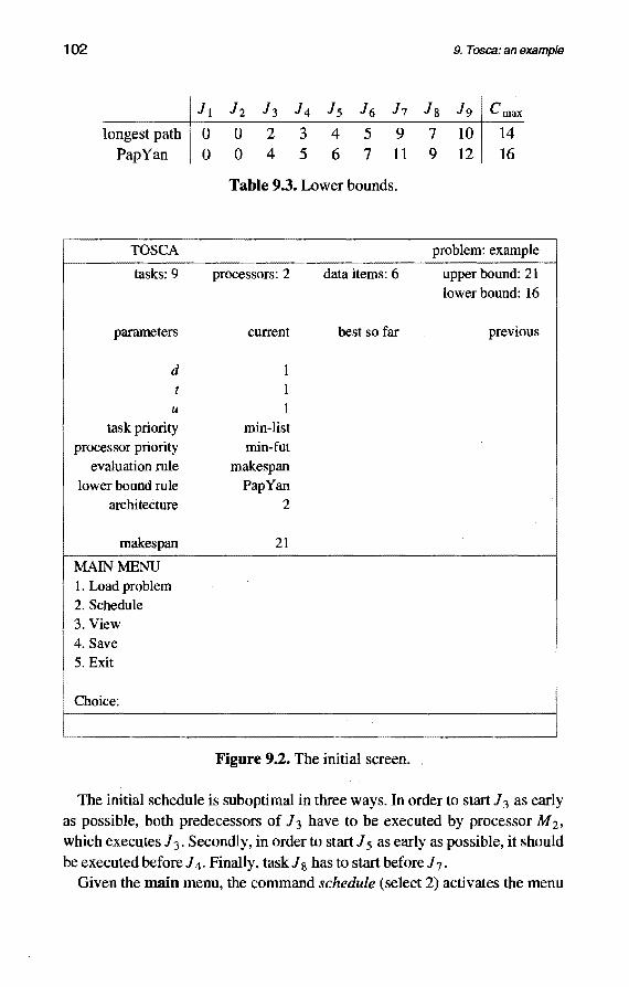
102
longest path PapYan
TOSCA
tasks: 9
parameters
d t
u task priority
processor priority evaluation rule
lower bound rule architecture
makes pan
MAIN MENU 1. Load problem 2. Schedule 3. View 4.Save 5.Exit
Jl
0 0
h h ]4 ls ]6 h 0 2 3 4 5 9 0 4 5 6 7 11
Table 9.3. Lower bounds.
processors: 2
current
1 1 1
min-list min-fut
makespan PapYan
2
21
data items: 6
best so far
Figure 9.2. The initial screen.
9. T osca: an example
ls ]9 Cmax
7 10 14 9 12 16
problem: example
upper bound: 21 lower bound: 16
previous
The initial schedule is suboptimal in three ways. In order to start J 3 as early as possible, both predecessors of J 3 have to be executed by processor M 2 ,
which executes J 3 . Secondly, in order to start J 5 as early as possible, it should be executed before J 4 • Finally, task J 8 has to start before J 7 •
Given the main menu, the command schedule (select 2) activates the menu

9. Tosca: an example 103
that allows for new choices of priority rules and evaluation rules. Changing the processor priority rule into, for instance, min-data and the evaluation rule into, for instance, PapYan will not help to construct a better schedule.
:~1 ~: 1 ==== 1'
31 '4 1,5 1-~-~---~n--;8--1- ,9 t--o 2 4 6 8 10 12 14 16 18 20 22
Figure 9.3a. List scheduling: initial schedule.
Figure 9.3b. List scheduling: max-tail, min-data.
:~1 113
1 1'51 ---------
1'71 t====== J2 J4
J9 Jl h I
Jg
0 2 4 6 8 10 12 14 16 18 20 22
Figure 9.3c. List scheduling: min-start, min-data.
Figure 9.3d. List scheduling: user defined priority rule.
Since the amount of work that has to be done after completion of J 5 is more than the work following J 4 , the choice of task priority rule max-tail will generate a schedule of length 20, as given in Figure 9.3b. Note that J 5 is executed beforeJ4 •
The choice of task priority rule min-start will execute J 8 before J 7 , because J 8 can start immediately following the completion of task J 6 . However, tasks J 4 and J 5 are placed in the wrong order again. The resulting schedule has make span 19 and is given in Figure 9 .3c.

104 9. Tosca: an example
If one searches for a better task priority rule, then one has to construct such a rule manually; the predefined priority rules will not help anymore. Such a user priority rule has to choose J 5 before J 4 and J 8 before J 7 • The user rule -(list-4)*(1ist-16/3)*(1ist-7) is such a priority rule. It considers the tasks in the order 2, 1, 3, 5, 4, 6, 8, 7, 9 and generates the schedule of length 18, given in Figure 9.3d.
Figure 9.3e. Bounded enumeration: d=3, t=2, and u=l.
Figure 9.3f. Bounded enumeration: d=3, t=2, and u
A schedule of length 18 can also be constructed by bounded enumeration with parameters d =3, t =2, and u = 1, and task priority rule max-tail, processor priority min-data, and evaluation rule PapYan; it is given in Figure 9.3e.
Finally, bounded enumeration with parameters d=3, t=2, and u=2 will yield a schedule of length 17; see Figure 9.3f. It is optimal since hand J 8
cannot be scheduled in parallel. An optimal schedule cannot be constructed by use of list scheduling. It is impossible to construct a processor priority rule that schedules tasks J 1 and J 2 on processor M 2 •

References

106 References
A.V. Aho, J.E. Hopcroft, J.D. Ullman (1988). Data structures and algorithms, Addison Wesley, Reading, MA.
M. Ahuja, Y. Zhu (1990). An O(nlogn) feasibility algorithm for preemptive scheduling of n jobs on a hypercube. Inform. Process. Lett. 35, 7-11.
F.D. Anger, J. Hwang, Y. Chow (1990). Scheduling with sufficiently loosely coupled processors. J. Parallel Distributed Comput. 9, 87-92.
T.S. Arthanri (1974). On some problems of sequencing and grouping, Dissertation, Indian Statistical Institute, Calcutta.
L. Bianco, P. Dell'Olmo, J. Blazewicz (1992). Scheduling multiprocessor independent tasks with dedicated processors and additional resources. Presentation, EURO XII- TIMS XXXI, Helsinki, 1992.
L. Bianco, P. Dell'Olmo, M.G. Speranza (1991). On scheduling independent tasks with dedicated resources. Presentation, 14th Int. Symp. Math. Programming, Amsterdam, August 5-9, 1991.
J. Blazewicz, P. Dell'Olmo, M. Drozdowski, M.G. Speranza (1992). Scheduling multiprocessor tasks on three dedicated processors. Inform. Process. Lett. 41,275-280.
J. Blazewicz, M. Drabowski, J. Weglarz (1986). Scheduling multiprocessor tasks to minimize schedule length. IEEE Trans. Comput. C-35, 389-393.
J. Blazewicz, M. Drozdowski, G. Schmidt, D. de Werra (1990). Scheduling independent two processor tasks on a uniform duo-processor system. Discrete Appl. Math. 28, 11-20.
J. Blazewicz, M. Drozdowski, G. Schmidt, D. de Werra (1992). Scheduling independent multiprocessor tasks on a uniform k-processor system, Report R30-92, Instytut Informatyki, Politechnika Poznanska, Poznan.
J. Blazewicz, G. Finke, R. Haupt, G Schmidt (1988). New trends in machine scheduling. European]. OperRes. 37,303-317.
J. Blazewicz, J.K. Lenstra, A.H.G. Rinnooy Kan (1983). Scheduling subject to resource constraints: classification and complexity. Discrete Appl. Math. 5, 11-24.
J. Blazewicz, J. Weglarz, M. Drabowski (1984). Scheduling independent 2-processor tasks to minimize schedule length. Inform. Process. Lett. 18, 267-273.
S.H. Bokhari (1981). On the mapping problem. IEEE Trans. Comput. C-30, 207-214.
G. Bozoki, J.P. Richard (1970). A branch-and-bound algorithm for the continuous-process task shop scheduling problem. AilE Trans. 2, 246-252.
R.E. Buten, V. Y. Shen ( 1973). A scheduling model for computer systems with two classes of processors, Proc. 1973 Sagamore Comput. Conference

References 107
Parallel Processing, 130-138. R.S. Chang, R.C.T. Lee (1988). On a scheduling problem where a job can be
executed only by a limited number of processors. Comput. Oper. Res. 15, 471-478.
Y.L. Chen, Y.H. Chin (1989). Scheduling unit-time jobs on processors with different capabilities. Comput. Oper. Res. 16, 409-417.
G.l. Chen, T.H. Lai (1988A). Scheduling independent jobs on hypercubes. Proc. Conf Theoretical Aspects of Computer Science, 273-280.
G.l. Chen, T.H.Lai (1988B). Preemptive scheduling of independent jobs on a hypercube.Infonn. Process. Lett. 28,201-206.
G.I. Chen, T.H. Lai (1991). Scheduling independent jobs on partitionable hypercubes. J. ParallelDistributed Comput.]2, 74-78.
P. Chretienne (1989) . .A polynomial algorithm to opti1llally schedule tasks on a virtual distributed system under tree-like precedence constraints. European J. Oper. Res. 43, 225-230.
P. Chretienne (1992). Task scheduling with interprocessor communication delays. European J. Oper. Res. 57, 348-354.
P. Chretienne, C. Picouleau (1991). The basic scheduling problem with interprocessor communication delays. RP9116, MASI, Institut Blaise Pascal, Universite Paris VI, Paris.
J.Y. Colin, P. Chretienne (1993). C.P.M. scheduling with small communication delays and task duplication. Oper. Res., to appear.
R.W. Conway, W.L. Maxwell, L.W. Miller (1967); Theory of scheduling, Addison-Wesley, Reading, MA.
G. Dobson, U.S. Karmarkar (1989). Simultaneous resource scheduling to minimize weighted flow times. Oper. Res. 37, 592-600.
J. Du, J. Y-T. Leung (1989). Complexity of scheduling parallel task systems. SIAM J. Discrete Math .. 2, 473-487.
H. El-Rewini, T.G. Lewis (1990). Scheduling parallel program tasks onto arbitrary target machines. J. parallel Distributed Com put. 9,.138-153.
M.J. Flynn (1966). Very high-speed computing systems. Proc. IEEE 54, 1901-1909.
M. Fujii, T. Kas!l@i, K. Ninomiya (1969, 1971). Optimal sequencing of two equivalent processors. SIAM J. Appl. Math. 17, 784-789; Erratum. SIAM J.
Appl. Math. 20,141. M.R. Garey, D.S. Johnson (1979). Computers and intractability: a guide to
the theory of NP-completeness, Freeman; San Francisco. A. Gerasoulis, T. Yang (1990, revision 1992). On the granularity and cluster
ing of directed acyclic task graphs. Report TR-153, Dept. Comput. ScL,

108 References
Rutgers University. M.C. Golumbic (1980). Algorithmic graph theory and perfect graphs,
Academic Press, New York. R.L. Graham ( 1966). Bounds for certain multiprocessing anomalies. Bell Sys
tem Tech. J. 45, 1563-1581. R.L. Graham, E.L. Lawler, J.K. Lenstra, A.H.G. Rinnooy Kan (1979). Optim
ization and approximation in deterministic sequencing and scheduling: a survey.Ann. Discrete Math. 5, 287-326.
J.A. Hoogeveen, J.K. Lenstra, B. Veltman (1992).1hree,four,five, six, or the complexity of scheduling with communication delays, Report BS-R9229, CWI, Amsterdam.
J.A. Hoogeveen, J.K. Lenstra, B. Veltman (1993). Minimizing makespan in a multiprocessor flow shop is strongly NP-hard, in preparation.
J.A. Hoogeveen, S.L. van de Velde, B. Veltman (1993). Complexity of scheduling multiprocessor tasks with prespecified processor allocations. Discrete Appl. Math., to appear.
T.C. Hu (1961). Parallel sequencing and assembly line problems. Oper. Res. 9, 841-848.
C.A.J. Hurkens (1992). Private communication. J.J. Hwang, Y.C. Chow, F.D. Anger, C.Y. Lee (1989). Scheduling precedence
graphs in systems with interprocessor communication times. SIAM J ~Comput.18, 244-257.
A. Jakoby, R. Reischuk (1992). The complexity of scheduling problems with communication delays for trees. Proc. Skandinavian Workshop on Algorithmic Theory 3, 165-177.
S.M. Johnson (1954). Optimal two- and three-stage production schedules with set -up times included. Nav. Res. Logist. Quart. 1, 61-68.
H. Jung, L. Kirousis, P. Spirakis (1989). Lower bounds and efficient algorithms for multiprocessor scheduling of dags with communication delays. Proc. ACM Symp. Parallel Algorithms and Architectures, 254-264.
H. Kellerer, G.J. Woeginger (1992). UET-Scheduling with constrained processor allocations. Comput. Oper. Res.19, 1-8.
S.J. Kim (1988). A general approach to multiprocessor scheduling, Report TR-88-04, Dept. Comput. Sci., University of Texas, Austin.
G.A.P. Kindervater, J.K. Lenstra (1988). Parallel computing in combinatorial optimization. Ann. Oper. Res. 14,245-289.
H. Krawczyk, M. Kubale (1985). An approximation algorithm for diagnostic test scheduling in multiprocessor systems. IEEE Trans. Comp. C-34, 869-872.
References 109
B. Kruatrachue, T. Lewis (1988). Grain size determination for parallel processing. IEEE Software, 23-32.
M. Kubale (1987). The complexity of scheduling independent two-processor tasks on dedicated processors. Inform. Process. Lett. 24, 141-147.
E.L. Lawler, J.K. Lenstra, A.H.G. Rinnooy Kan, D.B. Shmoys (1993). Sequencing and scheduling: algorithms and complexity. Handbooks in Operations Research and Management Science, Volume 4: Logistics of Production and Inventory, edited by S.C. Graves, A.H.G. Rinnooy Kan and P. Zipkin, North-Holland, Amsterdam.
C.Y. Lee, J.J. Hwang, Y.C. Chow, F.D. Anger (1988). Multiprocessor scheduling with interprocessor communication delays. Oper. Res. Lett. 7, 141-147.
H.W. Lenstra, Jr. (1983). Integer programming with a fixed number of variables. Math. Oper. Res. 8, 538-548.
J.K. Lenstra, A.H.G. Rinnooy Kan, P. Brucker (1977). Complexity of machine scheduling problems. Ann. Discrete Math. 1, 343-362.
J.K. Lenstra, M. Veldhorst, B. Veltman (1993). The complexity of scheduling trees with communication delays, in preparation.
K. Li, K.H. Cheng (1990). Static job scheduling in partitionable mesh con.;. nected systems. J. Parallel Distributed Comput. 10, 152-159.
H.X.Lin, H.J. Sips (1991).A distributed direct solver for the Diana finite elements system, ReportWP 1.4, Genesis, Esprit project.
E.L. Lloyd (1981). Concurrenttask systems; Oper; Res. 29, 189-201. S. Martello, P.Toth (1990). Knapsack problems: algorithms ami computer
implementations, Wiley, Chichester. R. McNaughton (1959). Scheduling with deadlines and loss functions.
Management Sci. 6, 1-12. R.H. Mohring (1989). Computationally tractable classes of ordered sets. I.
Rival (ed.) (1989). Algorithms and Order, Kluwer Academic, Dordrecht, 105-193.
C.H. Papadimitriou, J.D. Ullman (1987). A communication~time tradeoff.· SIAM J. Comput. 16, 639-646.
C.H. Papadimitriou, M. Yannakakis (1990). Towards an architectureindependent analysis of parallel algorithms. SIAM J. Comput. 19, 322-328.
C. Picouleau (1991A). Ordonnancement de taches de duree unitaire avec des delais de communication unitaires sur m processeurs. Report RP91/64, MASI, Institut Blaise Pascal, UniversiteParis VI, Paris.
C. Picouleau (1991B). Two new NP-complete scheduling problems with communication delays and unlimited number of processors. Report RP91/24,

110 References
MAS I, lnstitut Blaise Pascal, Universite Paris VI, Paris. C. Picouleau (1992). Etude de problemes d'optimisation dans les systemes
distribues. These de doctoral, Universite'Paris VI. V.J. Rayward-Smith (1987 A). UET scheduling with unit interprocessor com
munication delays. Discrete Appl. Math. 18, 55-71. V.J. Rayward-Smith (1987B). The complexity of preemptive scheduling
given interprocessor communication delays . . Inform. Process. Lett. 25, 123-125.
M.S. Salvador (1970). A solution to a special class of flow shop scheduling problems, Proc. Symp. Theory of Scheduling and its Applications. In S.E. Elmaghraby (ed.) (1973). Lecture Notes in Economics and Mathematical Systems 86, Springer, Berlin, 83-91.
V. Sarkar (1989). Partitioning and scheduling parallel programs for multiprocessors, Pitman, London.
A. Schrijver (1986). Theory of linear and integer programming, Wiley, Chichester.
J.T. Schwartz (1980). Ultracomputers. ACM Trans. Programming lAnguages and Systems 2, 484-521.
X. Shen, E.M. Reingold (1991). Scheduling on a hypercube. Inform. Process. Lett. 40, 323-328.
P,C. Treleaven, D.R. Brownbridge, R.P. Hopkins (1982). Data-driven and demand-driven computer architecture. Comput. Surveys 14, 93-143.
T.A. Varvarigou, V.P. Roychowdhury, T. Kailath (1992). Unpublished manuscript.
B. Veltman, B.J. Lageweg, J.K. Lenstra (1990). Multiprocessor scheduling with communication delays. Parallel Comput. 16, 173-182.
B. Veltman, B.J. Lageweg, J.K. Lenstra (1993). Tosca: a tunable off-line scheduling algorithm, in preparation.
Y. Zhu, M Ahuja (1990A). Preemptive job scheduling on a hypercube. Proc. Int. Conf Parallel Process., 301-304.
Y. Zhu, M Ahuja (1990B). Job scheduling on a hypercube. Proc. Int. Conf. Distributed Comput. Systems, 510-517.

Samenvatting

112 Multiprocessor scheduling with communication delays
Vele processoren maken Iicht werk moet het motto geweest zijn om parallelle computers te gaan ontwerpen en bouwen. Een processor is een rekenmachine die slechts een operatie tegelijkertijd kan uitvoeren. Een parallelle computer of multiprocessor is opgebouwd uit verscheidene processoren en kan dus een aantal taken tegelijkertijd verwerken.
De taken die een parallelle computer te verwerken krijgt zijn de modules waarin een parallel programma gepartitioneerd is. Tussen zulke taken bestaan in het algemeen informatie-afhankelijkheden, zodat zij niet zonder meer in iedere willekeurige volgorde verwerkt kunnen worden. Een schedule bepaalt voor elke taak het tijdstip waarop en de processoren waardoor deze uitgevoerd zal worden. Het streven is een snelle verwerking van de taken te garanderen.
In principe kan men een optimaal schedule vinden door te kiezen uit de aftelbare en vaak eindige verzameling van altematieven. Dit suggereert dat botweg compleet aftellen effectief zou zijn: genereer aile mogelijke oplossingen, bepaal hun kosten en kies een beste. Helaas is het aantal oplossingen vaak zo groot dat deze methode in de praktijk te veel tijd vergt. Men is gedwongen te zoeken naar snellere algoritrnen. De fundamentele vraag is of er een algoritrne bestaat dat een gegeven schedulingprobleem optimaal oplost in polynomiale tijd. Als dit het geval is dan beschouwen we zo'n algoritrne als 'snel' en is het probleem 'goed oplosbaar'. Voor andere problemen kan men aantonen dat het zeer onwaarschijnlijk is dat zo'n algoritrne bestaat; dit zijn de NP-lastige problemen. In de hoofdstukken 3-6 van dit proefschrift behandelen we de complexiteit van een aantal schedulingproblemen die optreden bij het gebruik maken van een multiprocessor. Deze problemen verschillen van hun klassieke varianten op een aantal punten. Wij hebben theoretisch onderzoek gedaan naar deze verschillen en hun consequenties.
Ten eerste dient men bij multiprocessorscheduling rekening te houden met communicatievertragingen. De informatie-atbankelijkheden leiden op natuurlijke wijze tot een precedentiestructuur op de taakverzameling; de verwerking van een taak kan pas beginnen als zijn voorgangers verwerkt zijn en als aile informatie aanwezig is op de processoren die de desbetreffende taak uit zullen voeren. In Hoofdstuk 3 bestuderen we het meest eenvoudige model met communicatievertragingen: elke taak vergt slechts ten processor voor executie en zowel verwerkingen als communicatievertragingen nemen een tijdseenheid in beslag. In het algemeen geldt dat zelfs dit eenvoudige model met communicatievertragingen al NP-lastig is.
Door middel van taakduplicatie kan men communicatievertragingen verkleinen of zelfs vermijden. Hoofdstuk 4 laat zien dat duplicatie een optimaal schedule kan verkorten met een factor gelijk aan ten hoogste het aantal

Samenvatting 113
processoren waaruit de multiprocessor bestaat. In bet voornoemde geval van verwerkingstijden en communicatievertragingen van een tijdseenheid lengte kan duplicatie slechts een factor twee helpen.
Een derde aspect betreft problemen waarbij bet mogelijk is dat een taak verscheidene processoren vergt voor executie. Zulke taken noemen we multiprocessortaken. Hoofdstuk 5 behandelt de complexiteit van bet toewijzen van starttijden aan multiprocessortaken, waarbij voor elke taak een van tevoren vastgestelde verzameling processoren is bepaald. Communicatie wordt nu buiten beschouwing gelaten. In bet algemeen geldt dat zelfs bet vinden van alleen starttijden een NP-lastig probleem is.
In Hoofdstuk 6 beschouwen we, evenals in de hoofdstukken 3-4, taken die slechts een processor voor executie vergen. De informatie-afhankelijkheden zijn zodanig dat de precedentiestructuur nit losse ketens van elk twee taken bestaat. De taken zonder voorgangers kunnen door twee processoreri verwerkt worden, maar de taken met voorgangers worden allen door een en dezelfde processor uitgevoerd. Het vinden van een schedule dat de maximale voltooiingstijd minimaliseert is een NP-lastig probleem, ook als menpreemptie toestaat. Preemptie is bet onderbreken van de executie van een taak om deze op een eventueellater tijdstip op dezelfde of een andere processor voort te zetten. Dit probleem is een variant van bet klassieke flow shop schedulingprobleem.
Uit de analyses van hoofdstukken 3-6 concluderen we dat bet onwaarschijnlijk is dat er een snel algoritme bestaat om bet algemene schedulingprobleem, met communicatievertragingen en multiprocessortaken, op te lossen. Men is genocidzaakt een benaderend algoritme te gebruiken. Tosca, een 'tunable off-line scheduling algorithm', belichaamt zo'n methode. Tosca is ontworpen om bet verwerken van parallelle programma's op gedistribueerde systemen te ondersteunen. Tosca kan gebruikt worden om prestaties van een programma in ontwikkeling te voorspellen; de kwaliteit van een schedule is een maat voor de kwaliteit van een gegeven decompositie van zo' n programma.
Hoofdstuk 7 geeft een beschrijving van de methodiek van Tosca. Tosca tracht een goed schedule te construeren binnen een aanvaardbaar tijdsbestek door middel van begrensde aftelling. In principe kan men een schedule construeren door de taken een voor een te voorzien van een starttijd en een processortoewijzing. De verschillende keuzemogelijkheden kunnen gerepresenteerd worden door middel van een aftellingsboom. Het proces van begrensde aftelling beschouwt, in tegenstelling tot complete aftelling, slechts een deel van deze boom. Het proces bestaat nit een aantal stappen. Per stap worden een taak en een processortoewijzing bepaald. Om deze te kunnen bepalen wordt een

114 Multiprocessor scheduling with communication delays
deelboom berekend. Drie parameters, twee prioriteitsregels en een ondergrensregel bepalen de vorm van deze deelboom. De bladeren van de deelboom worden geevalueerd met behulp van een evaluatieregel. Een taakprocessortoewijzing combinatie die een tak vastlegt waarin een blad van minimale waarde zit, wordt gekozen. Met behulp van de drie parameters geeft men een bovengrens aan de diepte en de breedte van de deelboom. Ben van de twee prioriteitsregels betreft de keuze van taken, de ander betreft de keuze van processortoewijzingen. Deze regels kunnen gekozen worden uit een gegeven verzameling of zijn door de gebruiker gemaakt. De gebruiker moet daarnaast een ondergrensregel en een evaluatieregel kiezen. Tosca is regelbaar daar bet de gebruiker zeggenschap geeft over de snelheid van de oplossingsmethode en de kwaliteit van de geproduceerde schedules.
Tosca is voorzien van een eenvoudige gebruikersinterface. Informatie wordt gepresenteerd op alfanumerieke wijze en de mens-machine interactie verloopt met behulp van menu's. We hebben Tosca getest op vier typen probleeminstanties: gelaagde precedentierelaties, serie-parallelle precedentierelaties, willekeurige precedentierelaties en twee precedentierelaties uit de praktijk. Bij de precedentierelaties genereerden we verwerkingstijden en informatie-afhankelijkheden. Hoofdstuk 8 beschrijft de gebruikersinterface, de probleemgeneratoren en de testresultaten.
Uit de testresultaten blijkt dat in bet algemeen list scheduling, waarbij in elke stap precies e'en taak en een processor toewijzing bekeken wordt, tamelijk goed werkt. Geavanceerdere vormen van begrensde aftelling nemen a1 vlug veel tijd in beslag en vinden slechts marginate verbeteringen. Het vinden van een optimaal schedule is, behalve voor kleine probleeminstanties, een hopeloze zaak.
Ofwel, bet is niet eenvoudig om vele processoren Iicht werk te Iaten maken.

Curriculum vitae
Bart Veltman werd geboren op 14 december 1963 te Reinheim (BRD). In 1982 behaalde hij het VWO-diploma aan het Elzendaalcollege te Boxmeer. Hij studeerde vanaf 1982 wiskunde aan de Katholieke Universiteit Nijmegen en voltooide deze studie met bet doctoraal diploma in 1987. Hij trad aansluitend als onderzoeker in opleiding in dienst van de Stichting Mathematisch Centrum en was tot december 1992 werkzaam bij bet Centrum voor Wiskunde en Informatica te Amsterdam. Hij was in de periode 1989-1991 tevens verbonden aan de Nederlandse Organisatie voor Toegepast Natuurwetenschappelijk Onderzoek te Delft en betrokken bij bet ParTool project aldaar. Sinds december 1992 is Bart als universitair docent in dienst van de Technische Universiteit Eindhoven.

STELLING EN
behorende bij h_et proefschrift
Multiprocessor scheduling with communication delays
van
Bart Veltman

I
Beschouw het cooperatieve spel (N, v ), met spelersverzameling N = { 1, ... , n} en waardefunctie v : 2N -'tlR, dat voldoet aan
(1) v({j})=O voor alle j EN, (2) v is superadditief, en (3) v(S)=!.reSht v(T)vooralleSE 2N.
Hier is 1t een permutatie van de spelersverzameling N en Sin de verzameling van componenten vanS onder deze permutatie. Voor zo'n cooperatief spel kan men de uitbetalingsregel ~: N -'tR definieren door
~(j) = 1h(v (Pju{j}) v(Pj)+v (Fju{j}) -v(Fj)) voor j EN.
Hier zijn Pi en Fi respectievelijk de voorgangers en opvolgers van j onder n. Deze uitbetalingsregel garandeert de stabiliteit van de grote coalitie N, zodat bet spel (N, v) gebalanceerd is.
I.J. Curiel, J.A.M. Potters, V. Rajendra Prasad, S.H. Tijs, B. Veltman (1993). Sequencing and cooperation. Oper. Res., te verschijnen.
II
Picouleau [1992] presenteert reducties om de NP-lastigheid aan te tonen van de volgende problemen:
(1) P lprec,c=1,pj=ll Cmax: een verzameling van n taken moet worden verwerkt door m processoren rekening houdend met informatie-afhankelijkheden en zowel verwerkingstijden als communicatievertragingen van een tijdseenheid lengte; bepaal een rooster zodanig dat de maximale voltooiingstijd wordt geminimaliseerd;
(2) P lprec,c=1,dup,pj=ll C max: de variant waarbij duplicatie is toegestaan; (3) P21prec,c=l,fix,pi=IICmax: de variant waarbij de taken verdeeld zijn over tw~ processoren;
(4) PI tree,c I C max: de variant waarbij informatie-afhank:elijkheden leiden tot een precedentierelatie in de vorm van een boom, met een onbeperkt aantal processoren, constante communicatievertragingen en willekeurige verwerkingstijden.
Zijn eerste drie reducties zijn niet polynomiaal; zijn vierde reductic is incorrect om een andere reden.
C. Picouleau (1992). Etude de proble'mes d'optimisation dans les systemes distribues. These de doctorat, Universite Paris VI, Paris.

m
De in stelling II genoemde problemen zijn NP-lastig.
J.A. Hoogeveen, J.K. Lenstra, B. Veltman (1992). Three, four, five, six, or the complexity of scheduling with communication delays, Report BS-R9229, CWI, Amsterdam.
J.A. Hoogeveen, S.L. van de Velde, B. Veltman (1993). Complexity of scheduling multiprocessor tasks with prespecified processor allocations. Discrete Appl. Math., te verschijnen.
A. Jakoby, R. Reischuk (1992). The complexity of scheduling problems with communication delays for trees. Proc. Skandinavian Workshop on Algorithmic Theory 3, 165-177.
IV
Het flow shop schedulingprobleem met twee fasen en in de tweede fase twee identieke parallelle machines,F2(l,P2) II Cmax• en de variant waarbij preemptie is toegestaan, F2(l,P 2) lpmtn I C max• zijn sterk NP-lastig.
J.A. Hoogeveen, J.K. Lenstra, B. Veltman (1993). Minimizing makespan in a multiprocessor flow shop is strongly NP-hard, in voorbereiding.
B. Veltman (1993). Dit proefschrift, hoofdstuk 6.
v
Schedulingtheorie Ievert een goed raamwerk voor bet analyseren van een parallel programma, rnits bet model waarmee zo'n programma beschreven wordt in hoge mate architectuuronafuankelijk is.
VI
Het dupliceren van taken kan in theorie een schedule sterk verkorten maar zal in praktijk meestal weinig effect hebben.

VII
Het is onmogelijk om met bebulp van een rondbreinaald een naadloze Mobiusband te breien. Wei kunnen er draaiingen in bet breiwerk optreden, maar door goed op te
passen is dit te voorkomen.
VIII
Cultuur is bet gebeel aan vormen waarin een object zicb tot de omgeving, de natuur, verboudt. Natuur is de omgeving waarbinnen cultuurvormen aanwezig zijn of gecultiveerd worden. Natuur en cultuur bestaan niet los van elkaar. Wat voor de een cultuur is, is voor de ander natuur. Cultuur is niet typiscb menselijk.
IX
Veel motorrijders zullen de eerste keer dat zij met een leeg zijspan een bocbt naar · recbts maken verrast worden door bet omhoogkomende bakje.