multiprocessor scheduling i: partitioned schedulingls12-€¦ · multiprocessor scheduling i:...
TRANSCRIPT

Multiprocessor Scheduling I:Partitioned Scheduling
Prof. Dr. Jian-Jia Chen
LS 12, TU Dortmund
22/23, June, 2015
Prof. Dr. Jian-Jia Chen (LS 12, TU Dortmund) 1 / 47

Outline
Introduction to Multiprocessor Scheduling
Partitioned Scheduling for Implicit-Deadline EDF Scheduling
Partitioned Scheduling for Implicit-Deadline RM Scheduling
Partitioned Scheduling for Constrained-Deadline DMScheduling
Partitioned Scheduling for Arbitrary-Deadline EDF Scheduling
Prof. Dr. Jian-Jia Chen (LS 12, TU Dortmund) 2 / 47

Multiprocessor Models
• Identical (Homogeneous): All the processors have the samecharacteristics, i.e., the execution time of a job is independent onthe processor it is executed.
• Uniform: Each processor has its own speed, i.e., the execution timeof a job on a processor is proportional to the speed of the processor.
• A faster processor always executes a job faster than slowprocessors do.
• For example, multiprocessors with the same instruction set butwith different supply voltages/frequencies.
• Unrelated (Heterogeneous): Each job has its own execution time ona specified processor
• A job might be executed faster on a processor, but other jobsmight be slower on that processor.
• For example, multiprocessors with different instruction sets.
Prof. Dr. Jian-Jia Chen (LS 12, TU Dortmund) 3 / 47

Scheduling Models
• Partitioned Scheduling:• Each task is assigned on a dedicated processor.• Schedulability is done individually on each processor.• It requires no additional on-line overhead.
• Global Scheduling:• A job may execute on any processor.• The system maintains a global ready queue.• Execute the M highest-priority jobs in the ready queue, where
M is the number of processors.• It requires high on-line overhead.
• Semi-Partitioned Scheduling:• Adopt task partitioning first and reserve time slots
(bandwidths) for tasks that allow migration.• It requires some on-line overhead.
Prof. Dr. Jian-Jia Chen (LS 12, TU Dortmund) 4 / 47

Course Material
• Ronald L. Graham: Bounds for certain multiprocessing anomalies.in Bell System Technical Journal (1966).
• Ronald L. Graham: Bounds on Multiprocessing Timing Anomalies.SIAM Journal of Applied Mathematics 17(2): 416-429 (1969)
• Dorit S. Hochbaum, David B. Shmoys: Using dual approximationalgorithms for scheduling problems theoretical and practical results.J. ACM 34(1): 144-162 (1987) (in textbook ApproximationAlgorithms by Vijay Vazirani, Chapter 10, not covered)
• Sanjoy K. Baruah, Nathan Fisher: The Partitioned MultiprocessorScheduling of Sporadic Task Systems. RTSS 2005: 321-329
• Jian-Jia Chen: Partitioned Multiprocessor Fixed-Priority Schedulingof Sporadic Real-Time Tasks. CoRR abs/1505.04693 (2015)
Prof. Dr. Jian-Jia Chen (LS 12, TU Dortmund) 5 / 47

Terminologies Used in Scheduling Theory
Graham’s Scheduling Algorithm Classification
• Classification: a|b|c• a: machine environment
(e.g., uniprocessor, multiprocessor, distributed, . . .)• b: task and resource characteristics
(e.g., preemptive, independent, synchronous, . . .)• c : performance metric and objectives
(e.g., Lmax, sum of finish times, . . .)
• Makespan problem:• M||Cmax
• The course material mainly comes from the traditionalmakespan scheduling in the context of minimizing themaximum utilization. (The paper by Baruah and Fisher inRTSS 2005 is an exception.)
• Imagine that the goal is to minimize the maximum utilizationafter task partitioning.
Prof. Dr. Jian-Jia Chen (LS 12, TU Dortmund) 6 / 47

Bin Packing Problem
• Given a bin size b, and a set of items with individual sizes, theobjective is to assign each item to a bin without violating thebin size constraint such that the number of allocated bins isminimized.
Prof. Dr. Jian-Jia Chen (LS 12, TU Dortmund) 7 / 47

Outline
Introduction to Multiprocessor Scheduling
Partitioned Scheduling for Implicit-Deadline EDF Scheduling
Partitioned Scheduling for Implicit-Deadline RM Scheduling
Partitioned Scheduling for Constrained-Deadline DMScheduling
Partitioned Scheduling for Arbitrary-Deadline EDF Scheduling
Prof. Dr. Jian-Jia Chen (LS 12, TU Dortmund) 8 / 47

Problem Definition
Partitioned Scheduling
Given a set T of tasks with implicit deadlines, i.e., ∀τi ∈ T,Ti = Di , the objective is to decide a feasible task assignment ontoM processors such that all the tasks meet their timing constraints,where Cim is the execution time of task τi on processor m.
• For identical multiprocessors: Ci = Ci1 = Ci2 = · · · = CiM .
• For uniform multiprocessors: each processor m has a speedsm, in which Cimsm is a constant.
• For unrelated multiprocessors: Cim is an independent variable.
Prof. Dr. Jian-Jia Chen (LS 12, TU Dortmund) 9 / 47

Hardness and Approximation of Partitioned Scheduling
NP-complete
Deciding whether there exists a feasible task assignment isNP-complete in the strong sense.
Proof
Reduced from the makespan or the bin packing problem.
• Approximations are possible, but what do we approximatewhen only binary decisions (Yes or No) have to be made?• Deadline relaxation: requires modifications of task specification• Period relaxation: requires modifications of task specification• Resource augmentation by speeding up: requires a faster
platform• Resource augmentation by allocating more processors: requires
a better platform
Prof. Dr. Jian-Jia Chen (LS 12, TU Dortmund) 10 / 47

Approximation Algorithms
An algorithm A is called an η-approximation algorithm (for aminimization problem) if it guarantees to derive a feasible solutionfor any input instance I with at most η times of the objectivefunction of an optimal solution. That is,
A(I ) ≤ ηOPT (I ),
where OPT (I ) is the objective function of an optimal solution.
Prof. Dr. Jian-Jia Chen (LS 12, TU Dortmund) 11 / 47

Largest-Utilization-First (LUF) - for EDF Scheduling
Input: T,M;1: re-index (sort) tasks such that Ci
Ti≥ Cj
Tjfor i < j ;
2: Ti ← ∅,Ui ← 0,∀m = 1, 2, . . . ,M;3: for i = 1 to N, where N = |T| do4: find m∗ with the minimum utilization, i.e., Um∗ = minm≤M Um;5: if Um∗ + Ci
Ti> 1 then
6: return ”The task assignment fails”;7: else8: assign task τi onto processor m∗, where
Um∗ ← Um∗ + Ci
Ti,Ti ← Ti ∪ {τi};
9: return feasible task assignment T1,T2, . . . ,TM ;
Properties
• The time complexity is O((N + M) log(N + M))
• If a solution is derived, the task assignment is feasible by using EDF.
Prof. Dr. Jian-Jia Chen (LS 12, TU Dortmund) 12 / 47
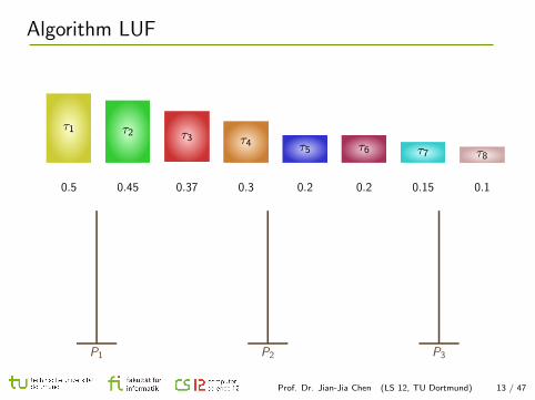
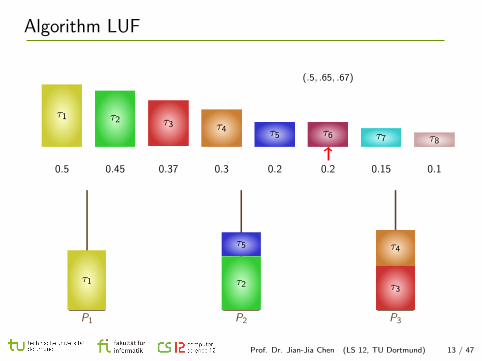
Algorithm LUF
τ1
0.5
τ2
0.45
τ3
0.37
τ4
0.3
τ5
0.2
τ6
0.2
τ7
0.15
τ8
0.1
(0, 0, 0) (.5, 0, 0) (.5, .45, 0) (.5, .45, .37) (.5, .45, .67) (.5, .65, .67) (.7, .65, .67) (.7, .8, .67)
P1 P2 P3
Prof. Dr. Jian-Jia Chen (LS 12, TU Dortmund) 13 / 47

Algorithm LUF
τ1
0.5
τ2
0.45
τ3
0.37
τ4
0.3
τ5
0.2
τ6
0.2
τ7
0.15
τ8
0.1
(0, 0, 0)
(.5, 0, 0) (.5, .45, 0) (.5, .45, .37) (.5, .45, .67) (.5, .65, .67) (.7, .65, .67) (.7, .8, .67)
P1 P2 P3
Prof. Dr. Jian-Jia Chen (LS 12, TU Dortmund) 13 / 47

Algorithm LUF
τ1
0.5
τ2
0.45
τ3
0.37
τ4
0.3
τ5
0.2
τ6
0.2
τ7
0.15
τ8
0.1
(0, 0, 0)
(.5, 0, 0)
(.5, .45, 0) (.5, .45, .37) (.5, .45, .67) (.5, .65, .67) (.7, .65, .67) (.7, .8, .67)
P1
τ1
P2 P3
Prof. Dr. Jian-Jia Chen (LS 12, TU Dortmund) 13 / 47

Algorithm LUF
τ1
0.5
τ2
0.45
τ3
0.37
τ4
0.3
τ5
0.2
τ6
0.2
τ7
0.15
τ8
0.1
(0, 0, 0) (.5, 0, 0)
(.5, .45, 0)
(.5, .45, .37) (.5, .45, .67) (.5, .65, .67) (.7, .65, .67) (.7, .8, .67)
P1
τ1
P2
τ2
P3
Prof. Dr. Jian-Jia Chen (LS 12, TU Dortmund) 13 / 47

Algorithm LUF
τ1
0.5
τ2
0.45
τ3
0.37
τ4
0.3
τ5
0.2
τ6
0.2
τ7
0.15
τ8
0.1
(0, 0, 0) (.5, 0, 0) (.5, .45, 0)
(.5, .45, .37)
(.5, .45, .67) (.5, .65, .67) (.7, .65, .67) (.7, .8, .67)
P1
τ1
P2
τ2
P3
τ3
Prof. Dr. Jian-Jia Chen (LS 12, TU Dortmund) 13 / 47

Algorithm LUF
τ1
0.5
τ2
0.45
τ3
0.37
τ4
0.3
τ5
0.2
τ6
0.2
τ7
0.15
τ8
0.1
(0, 0, 0) (.5, 0, 0) (.5, .45, 0) (.5, .45, .37)
(.5, .45, .67)
(.5, .65, .67) (.7, .65, .67) (.7, .8, .67)
P1
τ1
P2
τ2
P3
τ3
τ4
Prof. Dr. Jian-Jia Chen (LS 12, TU Dortmund) 13 / 47
Algorithm LUF
τ1
0.5
τ2
0.45
τ3
0.37
τ4
0.3
τ5
0.2
τ6
0.2
τ7
0.15
τ8
0.1
(0, 0, 0) (.5, 0, 0) (.5, .45, 0) (.5, .45, .37) (.5, .45, .67)
(.5, .65, .67)
(.7, .65, .67) (.7, .8, .67)
P1
τ1
P2
τ2
τ5
P3
τ3
τ4
Prof. Dr. Jian-Jia Chen (LS 12, TU Dortmund) 13 / 47

Algorithm LUF
τ1
0.5
τ2
0.45
τ3
0.37
τ4
0.3
τ5
0.2
τ6
0.2
τ7
0.15
τ8
0.1
(0, 0, 0) (.5, 0, 0) (.5, .45, 0) (.5, .45, .37) (.5, .45, .67) (.5, .65, .67)
(.7, .65, .67)
(.7, .8, .67)
P1
τ1
τ6
P2
τ2
τ5
P3
τ3
τ4
Prof. Dr. Jian-Jia Chen (LS 12, TU Dortmund) 13 / 47

Algorithm LUF
τ1
0.5
τ2
0.45
τ3
0.37
τ4
0.3
τ5
0.2
τ6
0.2
τ7
0.15
τ8
0.1
(0, 0, 0) (.5, 0, 0) (.5, .45, 0) (.5, .45, .37) (.5, .45, .67) (.5, .65, .67) (.7, .65, .67)
(.7, .8, .67)
P1
τ1
τ6
P2
τ2
τ5
τ7
P3
τ3
τ4
Prof. Dr. Jian-Jia Chen (LS 12, TU Dortmund) 13 / 47

Algorithm LUF
τ1
0.5
τ2
0.45
τ3
0.37
τ4
0.3
τ5
0.2
τ6
0.2
τ7
0.15
τ8
0.1
(0, 0, 0) (.5, 0, 0) (.5, .45, 0) (.5, .45, .37) (.5, .45, .67) (.5, .65, .67) (.7, .65, .67) (.7, .8, .67)
P1
τ1
τ6
U = 0.7
P2
τ2
τ5
τ7
U = 0.8
P3
τ3
τ4
τ8
U = 0.77
Prof. Dr. Jian-Jia Chen (LS 12, TU Dortmund) 13 / 47

Optimality of Algorithm LUF
Theorem
If an optimal assignment for minimizing the maximal utilization re-sults in at most two tasks on any processor, LUF is optimal.
Proof
The proof is omitted. If you are interested, you can take the proofas an exercise. The proof can be found from Graham’s paper.
Prof. Dr. Jian-Jia Chen (LS 12, TU Dortmund) 14 / 47

What Happens if Algorithm LUF Fails?
Assume that there exists a feasible task partition on M processors(for providing the analysis of resource augmentation).
• Suppose that Algorithm LUF fails when assigning task τj and Um form = 1, 2, . . . ,M is the utilization of processor m before assigning τj .
• Let Uopt be the utilization of the optimal assignment for minimizing themaximal utilization for tasks {τ1, τ2, . . . , τj}.
• By definition, 1 ≥ Uopt ≥∑j
i=1Ci/TiM
.
• Cj
Tj≤ 1
3Uopt : otherwise, there will be at most two tasks on any processors
in the optimal solution. ⇒ this contradicts the assumption thatAlgorithm LUF fails as it is optimal.
• Since Um∗ ≤ Um, we know that Um∗ ≤∑M
m=1UmM
=∑j−1
i=1Ci/TiM
.
• Therefore,
Cj
Tj+ Um∗ ≤
Cj
Tj(1− 1
M) +
j∑i=1
Ci/Ti
M≤(
4
3− 1
3M
)Uopt ≤
(4
3− 1
3M
).
Prof. Dr. Jian-Jia Chen (LS 12, TU Dortmund) 15 / 47

Algorithm LUF ∗: Resource Augmentation
Input: T,M;1: re-index (sort) tasks such that Ci
Ti≥ Cj
Tjfor i < j ;
2: Ti ← ∅,Ui ← 0,∀m = 1, 2, . . . ,M;3: for i = 1 to N, where N = |T| do4: find the processor m∗ with the minimum task utilization, i.e.,
Um∗ = minm Um;5: assign task τi onto processor m∗, where
Ui ← Ui + Ci
Ti,Ti ← Ti ∪ {τi};
6: return task assignment T1,T2, . . . ,TM with a speedup factormax{1,Um};
Prof. Dr. Jian-Jia Chen (LS 12, TU Dortmund) 16 / 47

Properties of LUF ∗
Theorem
If the input task set can be feasibly scheduled, Algorithm LUF ∗ de-rives a feasible task assignment/schedule by running the processorsat a speedup factor by at most 4
3 −1
3M .
Theorem
If the input task set cannot be feasibly scheduled by Algorithm LUF ,the task set is not schedulable by running at a slow-down factor
143− 1
3M
.
Prof. Dr. Jian-Jia Chen (LS 12, TU Dortmund) 17 / 47

Algorithm LUF+: Resource Augmentation on Processors
Input: T;1: re-index (sort) tasks such that Ci
Ti≥ Cj
Tjfor i < j ;
2: T1 ← ∅,U1 ← 0, M̂ ← 1;3: for i = 1 to N, where N = |T| do4: find a processor m∗ with Um∗ + Ci
Ti≤ 1;
5: if no such a processor exists then6: M̂ ← M̂ + 1,TM̂ ← ∅,UM̂ ← 0;
7: m∗ ← M̂;8: assign task τi onto processor m∗, where
Ui ← Ui + Ci
Ti,Ti ← Ti ∪ {τi};
9: return task assignment T1,T2, . . . ,TM̂ ;
Properties
• The time complexity is O(N logN) or O(N2), depending onthe fitting approaches.
• The resulting solution is feasible on M̂ processors.
Prof. Dr. Jian-Jia Chen (LS 12, TU Dortmund) 18 / 47

Different Fitting Approaches
4: find a processor m∗ with Um∗ + Ci
Ti≤ 1;
Fitting Strategies
• First-Fit: choose the feasible one with the smallest index
• Last-Fit: choose the feasible one with the largest index
• Best-Fit: choose the feasible one with the maximal utilization
• Worst-Fit: choose the feasible one with the minimal utilization
Suppose that we want to assign a task with utilization equal to 0.1.
P1 P2 P3 P4
0.6 0.70.5 0.65
First Fit Last FitBest FitWorst Fit
Prof. Dr. Jian-Jia Chen (LS 12, TU Dortmund) 19 / 47

Different Fitting Approaches
4: find a processor m∗ with Um∗ + Ci
Ti≤ 1;
Fitting Strategies
• First-Fit: choose the feasible one with the smallest index
• Last-Fit: choose the feasible one with the largest index
• Best-Fit: choose the feasible one with the maximal utilization
• Worst-Fit: choose the feasible one with the minimal utilization
Suppose that we want to assign a task with utilization equal to 0.1.
P1 P2 P3 P4
0.6 0.70.5 0.65First Fit
Last FitBest FitWorst Fit
Prof. Dr. Jian-Jia Chen (LS 12, TU Dortmund) 19 / 47

Different Fitting Approaches
4: find a processor m∗ with Um∗ + Ci
Ti≤ 1;
Fitting Strategies
• First-Fit: choose the feasible one with the smallest index
• Last-Fit: choose the feasible one with the largest index
• Best-Fit: choose the feasible one with the maximal utilization
• Worst-Fit: choose the feasible one with the minimal utilization
Suppose that we want to assign a task with utilization equal to 0.1.
P1 P2 P3 P4
0.6 0.70.5 0.65First Fit Last Fit
Best FitWorst Fit
Prof. Dr. Jian-Jia Chen (LS 12, TU Dortmund) 19 / 47

Different Fitting Approaches
4: find a processor m∗ with Um∗ + Ci
Ti≤ 1;
Fitting Strategies
• First-Fit: choose the feasible one with the smallest index
• Last-Fit: choose the feasible one with the largest index
• Best-Fit: choose the feasible one with the maximal utilization
• Worst-Fit: choose the feasible one with the minimal utilization
Suppose that we want to assign a task with utilization equal to 0.1.
P1 P2 P3 P4
0.6 0.70.5 0.65First Fit Last FitBest Fit
Worst Fit
Prof. Dr. Jian-Jia Chen (LS 12, TU Dortmund) 19 / 47

Algorithm LUF+: How Many Processors?
• Suppose that the processor used by Algorithm LUF+ is M̂ ≥ 2.
• Let m∗ be the processor with the minimum utilization.
• By the fitting algorithm, we know that Um + Um∗ > 1 and Um ≥ Um∗ forall the other processors ms.
• If Um∗ ≤ 0.5, by Um > 1− Um∗ , we know that
∑τi∈T
Ci
Ti≥ Um∗+
M̂∑m=1,m 6=m∗
Um ≥ M̂−1−(M̂−2)Um∗ = (M̂−2)(1−Um∗)+1 ≥ M̂
2.
• If Um∗ > 0.5, by Um ≥ Um∗ , we know that
∑τi∈T
Ci
Ti≥ Um∗ +
M̂∑m=1,m 6=m∗
Um ≥M̂
2.
Theorem
Algorithm LUF+ is a 2-approximation algorithm.
Prof. Dr. Jian-Jia Chen (LS 12, TU Dortmund) 20 / 47

Algorithm LUF Revisit: Upper and Lower Bounds
• Let m∗ be the processor with the maximum utilization among Mprocessors.
• Let τk be the last task that is added to m∗.
• Therefore, we know that Um ≥ Um∗ − Ck
Tkfor any other processor m.
• The lower bound of the maximum utilization to map T on Mprocessor is
LB ≥ max
{maxτi∈T
Ci
Ti,
∑τi∈T
Ci
Ti
M
}
⇒Um∗ ≤ Um +Ck
Tk≤∑M
m=1 Um
M+
Ck
Tk=
∑τi∈T
Ci
Ti
M+
Ck
Tk≤ 2LB.
• Therefore, we reach that
max
{maxτi∈T
Ci
Ti,
∑τi∈T
Ci
Ti
M
}= LB ≤ Um∗ ≤ 2LB.
Prof. Dr. Jian-Jia Chen (LS 12, TU Dortmund) 21 / 47

Outline
Introduction to Multiprocessor Scheduling
Partitioned Scheduling for Implicit-Deadline EDF Scheduling
Partitioned Scheduling for Implicit-Deadline RM Scheduling
Partitioned Scheduling for Constrained-Deadline DMScheduling
Partitioned Scheduling for Arbitrary-Deadline EDF Scheduling
Prof. Dr. Jian-Jia Chen (LS 12, TU Dortmund) 22 / 47
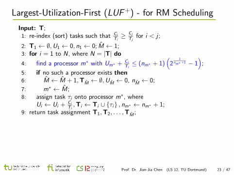
Largest-Utilization-First (LUF+) - for RM Scheduling
Input: T;1: re-index (sort) tasks such that Ci
Ti≥ Cj
Tjfor i < j ;
2: T1 ← ∅,U1 ← 0, n1 ← 0; M̂ ← 1;3: for i = 1 to N, where N = |T| do4: find a processor m∗ with Um∗ + Ci
Ti≤ (nm∗ + 1)
(2
1nm∗+1 − 1
);
5: if no such a processor exists then6: M̂ ← M̂ + 1,TM̂ ← ∅,UM̂ ← 0, nM̂ ← 0;
7: m∗ ← M̂;8: assign task τi onto processor m∗, where
Ui ← Ui + Ci
Ti,Ti ← Ti ∪ {τi} , nm∗ ← nm∗ + 1;
9: return task assignment T1,T2, . . . ,TM̂ ;
Properties
• The time complexity is O((N + M) log(N + M))
• If a solution is derived, the task assignment is feasible by using RM.
Prof. Dr. Jian-Jia Chen (LS 12, TU Dortmund) 23 / 47

A Simple Analysis
• The schedulability test Um∗ + CiTi≤ (nm∗ + 1)
(2
1nm∗+1 − 1
)is
upper bounded by 69.3%.
• According to the above analysis for EDF, we can also
conclude that the utilization is at least 0.693M̂2 .
• Therefore, the approximation factor of LUF+ is 20.693 ≈ 2.887.
Prof. Dr. Jian-Jia Chen (LS 12, TU Dortmund) 24 / 47

A More Precise Analysis
• If M̂ is 1, we know that∑τi∈T
CiTi≤ N(2
1N − 1).
• Suppose that the processor used by Algorithm LUF+ is M̂ ≥ 2.
• Let k be the index of the task, at which processor M̂ is allocated whenrunning LUF+. We only look at the iteration when i is k. Therefore,
Uk +∑τi∈Tm
Ui > (nm + 1)(
21
nm+1 − 1), ∀m = 1, . . . , M̂ − 1.
• By the sorting of the tasks, we also know that Ui ≥ Uk for any i ≤ k.
This also implies that∑τi∈Tm
Ui > nm
(2
1nm+1 − 1
).
• x(
21
x+1 − 1)
is an increasing function of x when x ≥ 1.
• Let q be the minimum number of tasks assigned on a processor beforetask τk , i.e., 1 ≤ q ≤ nm, ∀m = 1, . . . , M̂ − 1. The approximation factoris√
2 + 1 since
Uk +k−1∑i=1
Ui > (1 + (M̂ − 1)q)(
21
q+1 − 1)≥ M̂(
√2− 1) ≈ 0.414M̂.
Prof. Dr. Jian-Jia Chen (LS 12, TU Dortmund) 25 / 47

Remarks (Augmenting the Number of Processors)
Survey by Davis and Burns (ACM Computing Surveys, 2011):
Prof. Dr. Jian-Jia Chen (LS 12, TU Dortmund) 26 / 47

Outline
Introduction to Multiprocessor Scheduling
Partitioned Scheduling for Implicit-Deadline EDF Scheduling
Partitioned Scheduling for Implicit-Deadline RM Scheduling
Partitioned Scheduling for Constrained-Deadline DMScheduling
Partitioned Scheduling for Arbitrary-Deadline EDF Scheduling
Prof. Dr. Jian-Jia Chen (LS 12, TU Dortmund) 27 / 47

Definition and Theorem Recalled
For a task set, we say that the task set is with
• constrained deadline when the relative deadline Di is no morethan the period Ti , i.e., Di ≤ Ti , for every task τi , or
• arbitrary deadline when the relative deadline Di could belarger than the period Ti for some task τi .
Theorem
A task set T of independent, preemptable, periodic tasks can befeasibly scheduled (under EDF) on one processor if and only if
∀t ≥ 0,n∑
i=1
max
{0,
⌊t + Ti − Di
Ti
⌋}Ci ≤ t.
Prof. Dr. Jian-Jia Chen (LS 12, TU Dortmund) 28 / 47

Problem Definition
Partitioned Scheduling
Given a set T of tasks with arbitrary deadlines, the objective is todecide a feasible task assignment onto M processors such that allthe tasks meet their timing constraints, where Ci is the executiontime of task τi on any processor m.
I will only focus on speed-up (resource augmentation) factors forthe rest of the slides.
Prof. Dr. Jian-Jia Chen (LS 12, TU Dortmund) 29 / 47
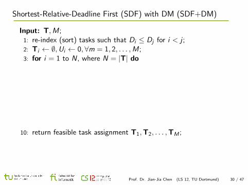
Shortest-Relative-Deadline First (SDF) with DM (SDF+DM)
Input: T,M;1: re-index (sort) tasks such that Di ≤ Dj for i < j ;2: Ti ← ∅,Ui ← 0, ∀m = 1, 2, . . . ,M;3: for i = 1 to N, where N = |T| do
4: for m = 1 to M do5: if task τi can be feasibly scheduled with Tm under DM
scheduling then6: assign task τi onto processor m and Tm ← Tm ∪ {τi};7: break;8: if τi is not assigned then9: return ”The task assignment fails”;
10: return feasible task assignment T1,T2, . . . ,TM ;
The used test can be an exact test (by using TDA) or autilization-based analysis.
Prof. Dr. Jian-Jia Chen (LS 12, TU Dortmund) 30 / 47

Shortest-Relative-Deadline First (SDF) with DM (SDF+DM)
Input: T,M;1: re-index (sort) tasks such that Di ≤ Dj for i < j ;2: Ti ← ∅,Ui ← 0, ∀m = 1, 2, . . . ,M;3: for i = 1 to N, where N = |T| do4: for m = 1 to M do5: if task τi can be feasibly scheduled with Tm under DM
scheduling then6: assign task τi onto processor m and Tm ← Tm ∪ {τi};7: break;
8: if τi is not assigned then9: return ”The task assignment fails”;
10: return feasible task assignment T1,T2, . . . ,TM ;
The used test can be an exact test (by using TDA) or autilization-based analysis.
Prof. Dr. Jian-Jia Chen (LS 12, TU Dortmund) 30 / 47

Shortest-Relative-Deadline First (SDF) with DM (SDF+DM)
Input: T,M;1: re-index (sort) tasks such that Di ≤ Dj for i < j ;2: Ti ← ∅,Ui ← 0, ∀m = 1, 2, . . . ,M;3: for i = 1 to N, where N = |T| do4: for m = 1 to M do5: if task τi can be feasibly scheduled with Tm under DM
scheduling then6: assign task τi onto processor m and Tm ← Tm ∪ {τi};7: break;8: if τi is not assigned then9: return ”The task assignment fails”;
10: return feasible task assignment T1,T2, . . . ,TM ;
The used test can be an exact test (by using TDA) or autilization-based analysis.
Prof. Dr. Jian-Jia Chen (LS 12, TU Dortmund) 30 / 47

Shortest-Relative-Deadline First (SDF) with DM (SDF+DM)
Input: T,M;1: re-index (sort) tasks such that Di ≤ Dj for i < j ;2: Ti ← ∅,Ui ← 0, ∀m = 1, 2, . . . ,M;3: for i = 1 to N, where N = |T| do4: for m = 1 to M do5: if task τi can be feasibly scheduled with Tm under DM
scheduling then6: assign task τi onto processor m and Tm ← Tm ∪ {τi};7: break;8: if τi is not assigned then9: return ”The task assignment fails”;
10: return feasible task assignment T1,T2, . . . ,TM ;
The used test can be an exact test (by using TDA) or autilization-based analysis.
Prof. Dr. Jian-Jia Chen (LS 12, TU Dortmund) 30 / 47

Constrained-Deadline: Failure when Using TDA
• Suppose that task τk is the first task that fails to be assigned on any ofthe M processors.
• Let T∗ be the set {τ1, τ2, . . . , τk−1}. Therefore,
∀m,∀t, with 0 < t ≤ Dk , Ck +∑τi∈Tm
⌈t
Ti
⌉Ci > t.
By taking a summation of all the m = 1, 2, . . . ,M inequalities with respect toany t, we have
∀t with 0 < t ≤ Dk , MCk +∑τi∈T∗
⌈t
Ti
⌉Ci > Mt.
By taking the negation, we know that if
∃t with 0 < t ≤ Dk , and Ck +∑τi∈T∗
⌈tTi
⌉Ci
M≤ t, (1)
then the SDF+DM by using TDA should succeed to assign task τk on one ofthe M processors.
Prof. Dr. Jian-Jia Chen (LS 12, TU Dortmund) 31 / 47

Constrained-Deadline: Schedulability Test for TDA
This is basically very similar to TDA with a minor difference by dividing thehigher-priority workload by M. Testing the schedulability condition of task τkcan be done by using the same strategy used in the k2U framework.We classify the k − 1 tasks in T∗ into two subsets.
• T∗1 consists of the tasks in T∗ with period smaller than Dk .
• T∗2 consists of the tasks in T∗ with period larger than or equal to Dk .
Let C ′k be defined as follows:
C ′k = Ck +∑τi∈T∗2
Ci
M.
Now, we can rewrite the condition as follows: if
∃t with 0 < t ≤ Dk and C ′k +∑τi∈T∗1
⌈tTi
⌉Ci
M≤ t,
then SDF+DM by using TDA should succeed to assign task τk on one of theM processors.
Prof. Dr. Jian-Jia Chen (LS 12, TU Dortmund) 32 / 47
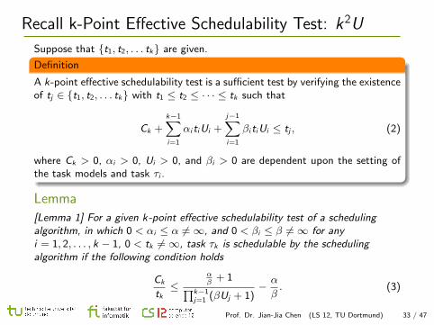
Recall k-Point Effective Schedulability Test: k2U
Suppose that {t1, t2, . . . tk} are given.
Definition
A k-point effective schedulability test is a sufficient test by verifying the existenceof tj ∈ {t1, t2, . . . tk} with t1 ≤ t2 ≤ · · · ≤ tk such that
Ck +k−1∑i=1
αi tiUi +
j−1∑i=1
βi tiUi ≤ tj , (2)
where Ck > 0, αi > 0, Ui > 0, and βi > 0 are dependent upon the setting ofthe task models and task τi .
Lemma[Lemma 1] For a given k-point effective schedulability test of a schedulingalgorithm, in which 0 < αi ≤ α 6=∞, and 0 < βi ≤ β 6=∞ for anyi = 1, 2, . . . , k − 1, 0 < tk 6=∞, task τk is schedulable by the schedulingalgorithm if the following condition holds
Ck
tk≤
αβ
+ 1∏k−1j=1 (βUj + 1)
− α
β. (3)
Prof. Dr. Jian-Jia Chen (LS 12, TU Dortmund) 33 / 47

Constrained-Deadline: Utilization-Base Test for TDA
TheoremIf ∏
τi∈T∗1(1 +
Ui
M) ≤ 2
1 +C ′k
Dk
,
then a constrained-deadline task τk is schedulable under SDF+DM by usingTDA.
Proof
• Let ti be⌊
TkTi
⌋Ti for τi ∈ T∗1.
• When using the k2U framework, we can reach the conclusion that
• αi = 1M , and 0 < βi ≤ 1
M
• tk is Dk and Ck (in the previous lemma) is C ′k .
• By adopting the above lemma, we reach the conclusion.
Prof. Dr. Jian-Jia Chen (LS 12, TU Dortmund) 34 / 47

Using Utilization-Based Test in SDF+DM
Instead of using the exact test, we can also use theutilization-based test (in the hyperbolic form) fordeadline-monotonic scheduling (see slide 30 in 11-k2u.pdf).Surprisingly, the result is the same as the case by using TDAanalysis.
• One of your exercise assignments is for the special case byusing the hyperbolic form in the schedulability test for RM.
Prof. Dr. Jian-Jia Chen (LS 12, TU Dortmund) 35 / 47

Summary of Existing Results
implicit deadlines constrained deadlines arbitrary deadlines
partitioned with EDF43− 1
3M(Graham
1969)3− 1
M(Baruah/Fisher 2006) 4− 2
M(Baruah/Fisher 2005)
(1 + ε)(Hochbaum/Shmoys1987)
2.6322 − 1M
(Chen/Chakraborty 2011)3− 1
M(Chen/Chakraborty 2011)
partitioned with DM(bin-packing) 7
4(Bur-
chard et al. 1995)3 − 1
M(Baker/Fisher/Baruah
2009)4− 2
M(Baker/Fisher/Baruah 2009)
(bin-packing) 1.5(Rothvoß2009)
2.84306 (Chen 2015) 3− 1M
(Chen 2015)
The above factors are for speed-up factors, except the two results in partitionedRM scheduling.
Prof. Dr. Jian-Jia Chen (LS 12, TU Dortmund) 36 / 47

Outline
Introduction to Multiprocessor Scheduling
Partitioned Scheduling for Implicit-Deadline EDF Scheduling
Partitioned Scheduling for Implicit-Deadline RM Scheduling
Partitioned Scheduling for Constrained-Deadline DMScheduling
Partitioned Scheduling for Arbitrary-Deadline EDF Scheduling
Prof. Dr. Jian-Jia Chen (LS 12, TU Dortmund) 37 / 47

Demand Bound Function Revisit for EDF
Define demand bound function dbf (τi , t) as
dbf (τi , t) = max
{0,
⌊t + Ti − Di
Ti
⌋}Ci = max
{0,
⌊t − Di
Ti
⌋+ 1
}Ci .
We need approximation to enforce polynomial-time schedulabilitytest.
dbf ∗(τi , t) =
{0 if t < Di
( t−DiTi
+ 1)Ci otherwise.
t0 1 2 3 4 5 6 7 8 9 10 11 12
dbf (τi , t)
Prof. Dr. Jian-Jia Chen (LS 12, TU Dortmund) 38 / 47

Demand Bound Function Revisit for EDF
Define demand bound function dbf (τi , t) as
dbf (τi , t) = max
{0,
⌊t + Ti − Di
Ti
⌋}Ci = max
{0,
⌊t − Di
Ti
⌋+ 1
}Ci .
We need approximation to enforce polynomial-time schedulabilitytest.
dbf ∗(τi , t) =
{0 if t < Di
( t−DiTi
+ 1)Ci otherwise.
t0 1 2 3 4 5 6 7 8 9 10 11 12
dbf (τi , t)
dbf ∗(τi , t)
Prof. Dr. Jian-Jia Chen (LS 12, TU Dortmund) 38 / 47
dbf (τi , t) ≤ dbf ∗(τi , t) ≤ 2dbf (τi , t)

Shortest Relative-Deadline First (SDF+EDF)
Input: T,M;1: re-index (sort) tasks such that Di ≤ Dj for i < j ;2: Ti ← ∅,Ui ← 0, ∀m = 1, 2, . . . ,M;3: for i = 1 to N, where N = |T| do
4: for m = 1 to M do5: if Ci
Ti+∑
τj∈Tm
Cj
Tj≤ 1 and
Ci +∑
τj∈Tmdbf ∗(τj ,Di ) ≤ Di then
6: assign task τi onto processor m and Tm ← Tm ∪ {τi};7: break;8: if τi is not assigned then9: return ”The task assignment fails”;
10: return feasible task assignment T1,T2, . . . ,TM ;
Prof. Dr. Jian-Jia Chen (LS 12, TU Dortmund) 39 / 47

Shortest Relative-Deadline First (SDF+EDF)
Input: T,M;1: re-index (sort) tasks such that Di ≤ Dj for i < j ;2: Ti ← ∅,Ui ← 0, ∀m = 1, 2, . . . ,M;3: for i = 1 to N, where N = |T| do4: for m = 1 to M do5: if Ci
Ti+∑
τj∈Tm
Cj
Tj≤ 1 and
Ci +∑
τj∈Tmdbf ∗(τj ,Di ) ≤ Di then
6: assign task τi onto processor m and Tm ← Tm ∪ {τi};7: break;
8: if τi is not assigned then9: return ”The task assignment fails”;
10: return feasible task assignment T1,T2, . . . ,TM ;
Prof. Dr. Jian-Jia Chen (LS 12, TU Dortmund) 39 / 47

Shortest Relative-Deadline First (SDF+EDF)
Input: T,M;1: re-index (sort) tasks such that Di ≤ Dj for i < j ;2: Ti ← ∅,Ui ← 0, ∀m = 1, 2, . . . ,M;3: for i = 1 to N, where N = |T| do4: for m = 1 to M do5: if Ci
Ti+∑
τj∈Tm
Cj
Tj≤ 1 and
Ci +∑
τj∈Tmdbf ∗(τj ,Di ) ≤ Di then
6: assign task τi onto processor m and Tm ← Tm ∪ {τi};7: break;8: if τi is not assigned then9: return ”The task assignment fails”;
10: return feasible task assignment T1,T2, . . . ,TM ;
Prof. Dr. Jian-Jia Chen (LS 12, TU Dortmund) 39 / 47

Feasibility
Theorem
If the tasks are partitioned successfully by using SDF+EDF Partition,EDF can feasibly schedule the tasks.
This is due to the feasibility analysis of the linear approximation ofthe demand bound functions.
Prof. Dr. Jian-Jia Chen (LS 12, TU Dortmund) 40 / 47

When Is SDF+EDF Always Successful?
Define that
• δmax is the maximum density, i.e., maxτi∈TCiDi
.
• µmax is the maximum utilization, i.e., maxτi∈TCiTi
.
• δmax and µmax are both less than or equal to 1.
• δsum is the maximum total dbf density, i.e.,maxt>0
∑τi∈T
dbf (τi ,t)t .
• µsum is the total utilization, i.e.,∑
τi∈TCiTi
.
Theorem
Any sporadic task set is successfully scheduled by SDF+EDF on Midentical processors, when
M ≥ 2δsum − δmax
1− δmax+µsum − µmax
1− µmax.
Prof. Dr. Jian-Jia Chen (LS 12, TU Dortmund) 41 / 47

Proof of Schedulability
Suppose that τk is not able to be assigned on any processor by SDF+EDF.
• Either CkTk
+∑τj∈T′m
Cj
Tj> 1 or Ck +
∑τj∈T′m
dbf ∗(τj ,Dk) > Dk .
• Suppose that among M processors, there are M1 processors, denoted byset M1, with Ck +
∑τj∈T′m
dbf ∗(τj ,Dk) > Dk .
• Therefore, by summing the inequalities together, we have
M1Ck +∑
τj∈T′m and m∈M1
dbf ∗(τj ,Dk ) > M1Dk .
⇒∑
τj∈T\{τk}2dbf (τj ,Dk ) > M1(Dk − Ck )
⇒∑τj∈T
2dbf (τj ,Dk ) > M1(Dk − Ck ) + Ck
divided by Dk ⇒
∑τj∈T
2dbf (τj ,Dk )
Dk
> M1Dk − Ck
Dk
+Ck
Dk
⇒2δsum > M1Dk − Ck
Dk
+Ck
Dk
• By above, we know that M1 <2δsum−
CkDk
1− CkDk
.
Prof. Dr. Jian-Jia Chen (LS 12, TU Dortmund) 42 / 47
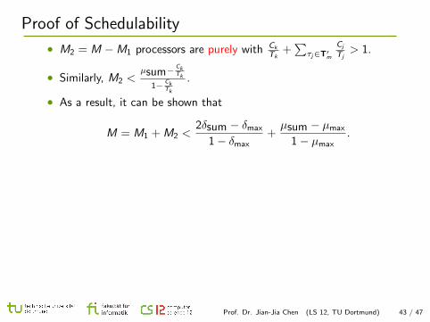
Proof of Schedulability
• M2 = M −M1 processors are purely with Ck
Tk+∑
τj∈T′mCj
Tj> 1.
• Similarly, M2 <µsum−
CkTk
1− CkTk
.
• As a result, it can be shown that
M = M1 + M2 <2δsum − δmax
1− δmax+µsum − µmax
1− µmax.
Prof. Dr. Jian-Jia Chen (LS 12, TU Dortmund) 43 / 47

Resource Augmentation
Theorem
If a sporadic task set is schedulable on M identical processors,SDF+EDF will successfully partition this task set upon a platformcomprised of M processors that are each (4 − 2
M ) times as fast asthe original.
Proof
The necessary condition to be schedulable on M identical processors is
δmax ≤ 1, µmax ≤ 1, µsum ≤ M, and δsum ≤ M.
If speeding up by 1γ satisfies M ≥ 2δsum−δmax
1−δmax+
µsum−µmax
1−µmax, it is feasible
by applying SDF+EDF. Therefore,
2δsum − δmax
1− δmax+µsum − µmax
1− µmax≤ 2Mγ − γ
1− γ+
Mγ − γ1− γ
=3Mγ − 2γ
1− γ
If M ≥ 3Mγ−2γ1−γ , the schedulability is enforced. ⇒ 4− 2
M ≤1γ .
Prof. Dr. Jian-Jia Chen (LS 12, TU Dortmund) 44 / 47

SDF+EDF for Constrained Deadlines
Theorem
Any sporadic task set with constrained deadlines is successfullyscheduled by SDF+EDF on M identical processors, when
M ≥ 2δsum − δmax
1− δmax.
Theorem
If a sporadic task set with constrained deadlines is schedulable on Midentical processors, SDF+EDF will successfully partition this taskset upon a platform comprised of M processors that are each (3− 1
M )times as fast as the original.
Main difference: Condition CiTi
+∑
τj∈T′mCj
Tj≤ 1 in Step 5 is always
enforced when Ci +∑
τj∈Tmdbf ∗(τj ,Di ) ≤ Di holds. ( ⇒ M2 is
always 0).
Prof. Dr. Jian-Jia Chen (LS 12, TU Dortmund) 45 / 47

Feasibility
Theorem
[Fisher and Baruah, RTSS 2005] The resource augmentation factorfor SDF+EDF has
• a 4− 2M resource augmentation factor for tasks with arbitrary
deadlines
• a 3− 1M resource augmentation factor for tasks with
constrained deadlines
Prof. Dr. Jian-Jia Chen (LS 12, TU Dortmund) 46 / 47

Feasibility
Theorem
[Fisher and Baruah, RTSS 2005] The resource augmentation factorfor SDF+EDF has
• a 4− 2M resource augmentation factor for tasks with arbitrary
deadlines
• a 3− 1M resource augmentation factor for tasks with
constrained deadlines
Theorem
[Chen and Chakraborty, RTSS 2011] The SDF+EDF has
• a 3− 1M resource augmentation factor for tasks with arbitrary
deadlines
• a 3e−1e − 1
M ≈ 2.6322− 1M resource augmentation factor for
tasks with constrained deadlines
Prof. Dr. Jian-Jia Chen (LS 12, TU Dortmund) 46 / 47

Summary of Existing Results
implicit deadlines constrained deadlines arbitrary deadlines
partitioned with EDF43− 1
3M(Graham
1969)3− 1
M(Baruah/Fisher 2006) 4− 2
M(Baruah/Fisher 2005)
(1 + ε)(Hochbaum/Shmoys1987)
2.6322 − 1M
(Chen/Chakraborty 2011)3− 1
M(Chen/Chakraborty 2011)
partitioned with DM(bin-packing) 7
4(Bur-
chard et al. 1995)3 − 1
M(Baker/Fisher/Baruah
2009)4− 2
M(Baker/Fisher/Baruah 2009)
(bin-packing) 1.5(Rothvoß2009)
2.84306 (Chen 2015) 3− 1M
(Chen 2015)
The above factors are for speed-up factors, except the two results in partitionedRM scheduling.
Prof. Dr. Jian-Jia Chen (LS 12, TU Dortmund) 47 / 47