Multiple Votes, Ballot Truncation and the Two-partySystem: An Experiment

September 2008

Abstract

Countries that elect their policy-makers by means of Plurality Voting tend to havea two-party system. We conduct laboratory experiments to study whether alternativevoting procedures yield a two-party system as well. Plurality Voting is compared withApproval Voting and Dual Voting, both of which allow voters to vote for multiplecandidates, but differ in whether voters are required to cast all their votes. We findthat both Plurality and Approval Voting yield a two-party system, whereas DualVoting may yield a multi-party system due to strategic voting. Voters’ ability totruncate ballots (not cast all their votes) is essential for maintaining the two-partysystem under Approval Voting.

Keywords: Strategic voting; Approval Voting; Ballot truncation; Duverger’s law.JEL Classification: C72, C9, D72.

Arnaud Dellis∗

Universite Laval and CIRPEEE-mail: arnaud.dellis@ecn.ulaval.ca

Sean D’Evelyn∗ and Katerina Sherstyuk∗

University of Hawai‘i - ManoaE-mail: sdevelyn@hawaii.edu, katyas@hawaii.edu

∗Financial support by the University of Hawaii Social Science Research Institute is gratefullyacknowledged. We would like to thank Thomas Palfrey, Thomas Rietz, Theodore Turocy, and theparticipants of the 2007 ESA North American Regional Meetings, the 2008 International Meetingof the Society for Social Choice and Welfare, and the 2008 ESA International Meetings for valuablecomments and discussion.

1

1 Introduction

Constitutional rules have a significant impact on economic policy-making. Empirical studies have

shown that a relationship exists between the effective number of parties and macro-economic

variables such as the levels of public deficit and income inequality or the composition of public

spending (Lizzeri and Persico, 2001; Persson and Tabellini, 2003). This paper contributes to

understanding how voting procedures affect the political party system. Using a laboratory setting,

we compare the effect several widely-discussed voting procedures have on the number of parties.

Countries that elect their policy-makers by means of Plurality Voting—i.e., the voting proce-

dure where every voter votes for one candidate—tend to have a two-party system. This empirical

regularity is known as Duverger’s law, which states that “the simple-majority single-ballot system

[i.e., Plurality Voting] favors the two-party system” (Duverger 1954; 217). This is certainly true

in the U.S., with the Democratic and Republican parties.1

Some political activists and scholars advocate replacing Plurality Voting with other voting

procedures that would allow or force people to vote for more than one candidate. Such electoral

reforms have been passed in several countries and municipalities (e.g. New Zealand, San Francisco)

and have recently been the object of referenda in two Canadian provinces (British Columbia and

Ontario). Electoral reforms are also advocated by several citizens associations (e.g. Citizens for

Approval Voting). The argument in support of such an electoral reform is based on the following

wasting-the-vote effect of Plurality Voting. In Plurality Voting elections, a voter whose most-

preferred candidate has no chance of winning the election would waste her vote by casting it for

that candidate. Such a voter has therefore an incentive to vote for another candidate that she

may like less but whose electoral prospects are better. This wasting-the-vote effect of Plurality

Voting is said to create a barrier to third-party candidates given that voters tend to anticipate

that third-party candidates have no chance of winning the election.2 The argument then goes that

if voters were given several votes to cast for the different candidates, they would no longer fear

wasting a vote on a third-party candidate, which would therefore help such a candidate.

Others advise against letting people vote for multiple candidates. They warn that lifting

the barriers to third-party candidates would trigger a proliferation of parties and the dangers

of multipartism. For example, multipartism could give rise to coalition governments and the

inefficiencies that are often associated with this form of government, e.g. Roubini and Sachs

(1989). Since candidates can be elected with less votes in a multi-party system than in a two-party1There are a few exceptions however. For example, Canada has a multiparty system despite holding its

political elections under Plurality Voting. Riker (1982) explains the Canadian exception by the geographicconcentration of third-party voters.

2For theoretical contributions explaining Duverger’s law by the wasting-the-vote effect of PluralityVoting, see e.g. Palfrey 1989; Feddersen 1992; Myerson and Weber 1993; Fey 1997.

2

system, inequality could then be on the rise. This is because candidates would have an incentive

to target electoral promises to smaller groups of voters, e.g. Lizzeri and Persico (2005).

This paper contributes to the debate whether letting people vote for multiple candidates would

obliterate the two-party system. We say that there is a two-party system if no more than two

parties get their candidate elected with positive probability. Another common formal interpretation

of Duverger’s law is that in Plurality Voting elections, only two parties receive votes; e.g. Palfrey

(1989), Feddersen (1992), Myerson and Weber (1993). As Myatt (2007) points out however, it is

rare to observe a full concentration of votes on only two candidates; trailing candidates usually

receive a non-negligible share of the votes. This is confirmed by Hirano and Snyder (2007) who

provide empirical evidence that in Plurality Voting elections third-party candidates receive votes.

Our definition of a two-party system relies on the latter observation, and focuses on the upper-

bound on the number of viable competitors.

Contrary to conventional wisdom, the theoretical results in Dellis (2007) suggest that letting

people vote for multiple candidates need not obliterate the two-party system that characterizes

Plurality Voting elections. Dellis studies scoring rules, a large class of commonly used and studied

voting procedures (e.g. Cox 1987; Myerson 2002) that include Plurality Voting and many of its

frequently-discussed alternatives. Under a scoring rule, every voter has a set of scores to cast for

the different candidates and the candidate whose total score is the highest wins the election. All

scoring rules differ only in the type of ballot a voter can cast.3 Dellis identifies two classes of

scoring rules which, under standard assumptions on voter preferences, yield a two-party system.

One class includes all the scoring rules under which every voter has a unique maximal top-score

vote to cast; Plurality Voting belongs to this class.4 The other class of scoring rules that yield

a two-party system consists of all the scoring rules that admit truncated ballots, that is, do not

force voters to cast all their scores.5 An example of such scoring rule is Approval Voting, under

which a voter can vote for as many candidates as she wishes. Finally, all scoring rules that belong

to neither of these two classes risk the breakdown of the two party system. Examples are: Dual

Voting, under which a voter must vote for exactly two candidates; and Negative Voting, under

which a voter must vote for all except one of the candidates.

This paper reports the results of a laboratory experiment that compares three distinct scoring3Part of the appeal of the scoring rules for study purposes is related to the way a voting procedure is

defined. More specifically, a voting procedure is defined by three elements: (1) the ballot structure, i.e.,the type of ballot a voter can cast; (2) the allocation rule, i.e., the way it transforms votes into seats; and(3) the district magnitude, i.e., the number of seats in a district. By comparing scoring rules we can isolatethe effect of the ballot structure since scoring rules differ only in this variable.

4Other examples of such scoring rules are the Borda Count and Cumulative Voting. We do not considerthese rules in the present study.

5Ballot truncation is often referred to in the literature as partial absention.

3

rules in their effect on the two-party system: Plurality Voting, Approval Voting and Dual Voting.

Plurality Voting is chosen as a benchmark; it is also an example of a scoring rule that requires

unique maximal top-score vote to cast and thus belongs to the first class identified by Dellis (2007).

Approval Voting is chosen as one of the most often discussed alternatives to Plurality Voting (e.g.,

Brams 2007; Forsythe et al. 1996; Laslier and Van der Straeten 2008);6 it is also a scoring rule

that admits truncated ballots and thus belongs to the second class of scoring rules yielding a two-

party system as identified by Dellis (2007). Finally, Dual Voting is chosen as a scoring rule that

belongs to neither class and thus may lead to a multi-party system. It is also identical to Approval

Voting in the three-candidate setting that we study, except it does not admit truncated ballots.

This allows us to test whether Dual Voting may lead to a different number of winning parties as

compared to Approval Voting, and thus consider the role of ballot truncation in Approval Voting

procedure.

Most experimental work on voting in elections focuses on Plurality Voting, and studies voter

behavior under incomplete information and the informational or coordinating role of past elections

(e.g., Collier et al. 1987; Forsythe et al. 1993), pre-election polls, ballot position, campaign

contributions (e.g., Forsythe et al. 1993; Rietz et al. 1998) or sequential voting (e.g., Morton and

Williams 1999; Battaglini et al. 2007).7 Several studies compare voting rules in multi-candidate

elections; see Rietz (2003) and Palfrey (2006) for comprehensive surveys. Rapoport et al. (1991)

study sincere and strategic voting under Plurality and Approval Voting; they report that both types

of voting are common in their experiments. Forsythe et al. (1996) compare vote coordination in

three-candidate elections under Plurality Voting, Approval Voting and the Borda Count. They

find that three-way ties among candidates occur more frequently under Approval Voting and the

Borda Count than under Plurality Voting. Unlike Forsythe et al. (1996), our analysis considers

situations where all voters’ utility functions are concave over the policy space.8

The present paper yields several interesting results. First, we clearly observe that the voting

procedures differ in their effect on the two-party system. In our experiment both Plurality and

Approval Voting gave rise to a two-party system: in almost all elections at most two candidates

tied for the first place, and three-way ties among candidates occurred very rarely. By contrast,6Approval Voting is currently used by several academic and professional associations to elect their

officers.7Our focus here is on voting behavior in elections; we therefore do not review many other important

contributions to experimental political science such as candidate spatial competition, committee decisionmaking, information aggregation in juries, or voter turnout and participation; see, e.g., Palfrey (2006).

8Blais et al. (2008) study strategic voting behavior in five-candidate elections under Plurality Voting,Plurality Runoff, Approval Voting and Single Transferable Vote. They conclude that voters tend to behavestrategically provided strategic computations are not too involved, as when the election is held underPlurality Voting or Approval Voting. Unlike Blais et al. (2008), our analysis considers how the possibilityto truncate one’s ballot affects voters’ strategic behavior and, in turn, the party structure.

4

Dual Voting gave rise to multipartism: three-way ties occurred in a significant number of elections.

We also observe that, under Plurality and Approval Voting elections, the same two candidates

were repeatedly among those who had a positive chance of winning elections; the third candidate

was almost never in the winning set. At the same time, all three candidates had a positive and

significant chance of being in the winning set when the elections were held under Dual Voting.

This gives additional evidence for the two-party system under Plurality and Approval Voting, and

the multiparty system under Dual Voting.

We further show that the breakdown of the two-party system in Dual Voting elections is the

result of strategic voting behavior. Dellis attributes the possibility of multipartism in Dual Voting

elections to the fact that those voters who decide to vote cannot truncate their ballots and are

thus forced to vote for two candidates. The voters who prefer a three-way tie to the outright

election of their second most-preferred candidate are then led to cast one of their two votes for

their most-preferred candidate and dump their second vote on their least-preferred candidate; thus,

an equilibrium that involves a three-way tie among candidates may exist. By contrast, such vote

dumping should not occur in Plurality and Approval Voting elections because here voters can

truncate their ballots and therefore are not forced to vote for more than one candidate. Consistent

with this argument, we find strong evidence of strategic vote dumping in Dual Voting elections,

but not in Plurality and Approval Voting elections. This establishes that the voters’ ability to

truncate ballots is essential for maintaining the two-party system under Approval Voting.

Our experiments also yield some unanticipated results. Notable among these is a strong pres-

ence of the middle candidate–i.e., the candidate whose platform lies between the platforms of the

other two candidates–among winners under all three voting procedures. Due to multiplicity of

equilibria, this focal effect of the middle candidate is not anticipated (even though it is not ruled

out either) by the Nash Equilibrium theory, even if the voters are assumed not to use weakly

dominated voting strategies. Interestingly, theories of boundedly rational behavior, such as the

Quantal Response Equilibrium and level-k reasoning, do not explain the overwhelming precedence

of the middle candidate in the winning sets for our setting either.

Finally, we gain some insights into individual voting behavior and voter ability to understand

different voting rules. A common practice in the formal voting literature is to assume that people

do not cast weakly dominated ballots, that is, ballots that can never affect the electoral outcome

in the person’s favor compared to some other ballot. Consistent with previous experiments (e.g.

Rapoport et al., 1991; Forsythe et al., 1996), we find strong evidence in support of this assumption

in the case of Plurality Voting. However, we find that sizeable numbers of weakly dominated

ballots were cast in Dual and Approval Voting elections. Moreover, consistent with Rapoport

et al. (1991), we find that this phenomenon was rather widespread and persistent with subject

5

experience in the case of Approval Voting. This contrasts with Laslier and Van der Straeten (2008),

who report, based on a field experiment in France, that the principle of Approval Voting was easily

understood and accepted by French voters. Our findings suggest that Approval Voting may be

more complex than it seems. Further, such evidence puts in question a common practice in the

formal comparative voting literature, the practice of imposing the weak undominance refinement

indiscriminately across all voting procedures.

As any study, this work has some limitations. First, we establish that in some cases the two-

party system may break down under voting procedures that do not admit truncated ballots, such as

Dual Voting. We do not address the question of how likely multipartism is to take place under Dual

Voting under a wide range of voter distributions and possible candidate positions. Our objective,

however, is to demonstrate that a single feature of a voting rule, such as admissibility of truncated

ballots, may have a large effect on the two-party system in some cases; thus, voters’ ability to

truncate ballots is essential for maintaining the two-party system under Approval Voting. Second,

we focus on voter behavior and not candidate behavior. Adding the candidate competition aspect

in comparing different voting procedures is important but is left for further research.9 Third, we

are looking at experimental elections with a relatively small number of voters. The implications of

our results for large elections are discussed in Section 5 at the end. Fourth, we assume all voters

have complete information about the candidates’ and other voters’ positions, and do not consider

a more realistic setting with incomplete information. All these issues are important but we feel

that an experimental test in a simple setting, such as the one we consider in this study, is essential

before one could move on to more complex and realistic settings.

The remainder of the paper is organized as follows. Section 2 outlines the theoretical model

that forms the basis for our experiment. Section 3 describes the experimental design. Section 4

presents the results. Section 5 concludes.

2 Model

A community of N citizens must elect a representative to implement a policy such as a tax rate or

the level of public spending. The set of policy alternatives X is a non-empty interval on R.10 We

assume that citizen �’s policy preferences can be represented by a strictly concave utility function

u� (·), and we define x� ≡ arg maxx∈X

u� (x) as citizen �’s (unique) ideal policy. All citizens are expected

utility maximizers.9A number of theoretical contributions explain Duverger’s law by the strategic behavior of par-

ties/candidates: e.g. Palfrey, 1984; Weber, 1992 and 1998; Morelli, 2004; Callander, 2005; Fey, 2007.10Empirical works have shown that citizens’ preferences over the different issues tend to be strongly

correlated. It has therefore been suggested that assuming a unidimensional policy space need not berestrictive, e.g. Cox (1990), Poole and Rosenthal (1991) and Hinich and Munger (1994).

6

Let C be a non-empty set of candidates, and let xi denote candidate i’s platform, i.e., the

policy that candidate i is committed to implement if elected. We assume that each candidate is

put on the ballot by a different party.

The citizens vote for candidates simultaneously. The election is held under a scoring rule,

where each citizen is given a set of point-scores {s1, ..., sC} to cast for the different candidates,

with s1 ≥ s2 ≥ ... ≥ sC . The candidate who receives the most points wins the election. If

several candidates tie for first place, each of these candidates is elected with an equal probability.

We denote citizen �’s (pure) voting strategy by α� (C) =(α�

1 (C) , ..., α�C (C)

), where α�

i (C) is the

point-score that citizen � casts for candidate i. In this paper we consider three scoring rules: (1)

Plurality Voting (hereafter PV), under which a feasible ballot is any permutation of the vector

(1, 0, ..., 0); (2) Dual Voting (hereafter DV), under which a feasible ballot is any permutation of

the vector (1, 1, 0, ..., 0); and (3) Approval Voting (hereafter AV), under which a feasible ballot is

any permutation of any one of the following vectors (1, 0, ..., 0), (1, 1, 0, ..., 0), ..., (1, ..., 1). Citizens

can also abstain from voting, in which case the ballot is the null vector.11

Since in our model each candidate is identified with a different party, we say that a voting

procedure yields a two-party system if in any Nash equilibrium, defined in the usual way, at most

two candidates (parties) tie for first place. The following proposition, which follows from Dellis

(2007), identifies sufficient conditions for a scoring rule to yield a two-party system.

Proposition 1 Consider a non-empty set of candidates. A scoring rule yields a two-party system

if the voter

1. has a unique top-score vote to cast, i.e., s1 �= s2; or

2. can truncate his ballot, i.e., a ballot is feasible if it is a permutation of any of the following

vectors (0, ..., 0), (s1, 0, ..., 0), (s1, s2, 0, ..., 0), ..., (s1, ..., sC).‖

PV (AV) satisfies the first (second) condition of Proposition 1 and, therefore, yields a two-

party system. By contrast, DV satisfies none of the conditions of Proposition 1 and may yield

multipartism, as illustrated next. Consider an example displayed in Figure 1. There are three

candidates located on the interval [1, 10]. One candidate is located at 1 (labeled “Green”), another

one at 3 (labeled “Orange”) and the third one at 9 (labeled “Blue”). There are six voters whose

ideal points are indicated by crosses on the figure. There are two voters with ideal point 2, two

voters with ideal point 6, and two voters with ideal point 10. The voters at 2 are indifferent

between Green and Orange, and prefer these candidates to Blue; the voters at 6 are indifferent11Observe that under AV, voting for all candidates – i.e., the ballot (1, ..., 1) – is equivalent to abstaining

from voting.

7

between Orange and Blue, and prefer them to Green; and the voters at 10 prefer Blue to Orange

to Green.

INSERT FIGURE 1 ABOUT HERE

It is straightforward to check that in any Nash equilibrium under Plurality or Approval Voting,

at most two candidates tie for first place, implying a two-party system. In contrast, under Dual

Voting, an equilibrium exists where all three candidates tie for first place, implying multipartism.

This equilibrium under Dual Voting may occur due to strategic behavior on the part of the voters

located at 10. To see this, note that the voters at 2 and 6 cannot benefit from misrepresenting their

preferences and, therefore, should vote for the two candidates who are closest to their position;

this generates two votes for Green, four votes for Orange, and two votes for Blue. Voter at 10 may

vote for Blue and Orange, in which case Orange wins outright. Or, each voter at 10 may vote for

Blue and Green, in which case all three candidates tie for first place. For a payoff structure as

in Table 1, voters at position 10 get a higher expected payoff from the three-way tie than from

Orange winning outright and, therefore, have an incentive to cast one of their votes for Blue, their

most-preferred candidate, and “dump” their other vote on Green, their least preferred candidate.

Note that this incentive does not exist under Plurality and Approval Voting since neither of these

two voting rules forces people to vote for multiple candidates.

While this example appears specific, it is illustrative of the general properties of the voting

rules we study. Below, we describe an experiment that was designed to test the above predictions.

3 Experimental design

Experimental subjects in the roles of voters participated in sequences of experimental elections

over three candidates. There were three experimental treatments corresponding to three voting

procedures: Plurality Voting (vote for exactly one candidate), Dual Voting (vote for exactly two

candidates) and Approval Voting (vote for as many of the candidates as wished). The motivation

for the choice of these voting procedures is explained in detail in Sections 1 and 2 above. Under

all three voting procedures, voters were also given the option to abstain from voting.12

12We gave this option to ensure symmetry across all three voting procedures. Indeed, without thisoption, participants could have abstained from voting under Approval Voting, but not under Pluralityand Dual Voting. This is because under Approval Voting, voting for all candidates is equivalent to voteabstention. In fact, our participants seldomly abstained, which suggests that our results would have beensimilar had we not allowed participants to abstain from voting. In PV sessions abstention was chosenin only 9 out of 1,440 voting decisions. In AV sessions abstention was chosen in 3 out of 1,392 votingdecisions while voting for all three candidates–a voting behavior which, as noted above, is equivalent tovote abstention–was chosen 68 times. Finally, in DV sessions abstention was chosen in 62 out of 1,392voting decisions.

8

There were twelve experimental sessions, with four independent sessions held under each of

the three voting procedures. The voting procedure was held constant within a session. There were

twelve subjects in each session. A session consisted of seven or eight voting series, with four election

periods per series.13 The division of a session into series was meant to provide some opportunity

for convergence within a series, while limiting dynamic strategic behavior. At the beginning of each

series of election periods, the participants were randomly matched into two groups of six voters

each. Within each group, the participants’ ideal points were randomly assigned among the voters’

locations as described in Figure 1. The colors associated with the candidates (Green, Orange and

Blue) were also randomly assigned among the candidates’ locations described in the figure.14 The

locations of the candidates and of the different participants in the group were common knowledge.

However, the identity and the individual voting history of the other participants in the group was

not revealed. The instructions (included in Appendix A) used a neutral terminology with the

candidates referred to as “alternatives”.

In each election period, an independent election was held within each group. Participants

placed votes for the candidates according to the given voting procedure. The candidate who

received the most votes in the group won the election. Ties were broken randomly. After all par-

ticipants had placed their votes, each participant’s screen reported the vote totals of the candidates,

the winning candidate in their group, and the participant’s payoff from the election.

Table 1 reports the payoffs that a participant received from the election depending on his

location and on the location of the elected candidate.

INSERT TABLE 1 ABOUT HERE

The payoff matrix was constructed from strictly concave distance utility functions. Further,

the payoffs of a participant at 10 were constructed so that her expected payoff was larger when

all three candidates tied for first place than when Orange won outright; this was necessary for a

three-way-tie equilibrium to exist under DV. In addition, to address possible concerns for ‘equity’

across participants, affine transformations of the payoffs were taken so that at each position the13The first session under DV and AV and the first two sessions under PV had eight series of four election

periods. As it became obvious that there were no significant differences between the seventh and the eighthseries, we shortened all subsequent sessions to seven series of election periods so that no session lasts morethan two hours. We include in our analysis the data from these eighth series of election periods. Ourresults are not sensitive to this inclusion.

14During each session we also alternated the line-up described in Figure 1 with a line-up symmetric tothis, where candidates were located at 2, 8 and 10, and participants were located at 1, 5 and 9. Thetwo line-ups were used to keep the participants from getting accustomed to the same setting, and also tocheck whether the results are different depending on whether the line-up involved a left extremist (i.e.,a candidate located at 1) or a right extremist (i.e., a candidate located at 10). The data indicate nodifference in participants’ behavior across the two settings. We will therefore pool the data and presentthe results in the context of the line-up described in Figure 1.

9

payoffs over all three candidates summed up to a similar number.15 The payoff matrix was common

knowledge to all participants.

The Nash equilibrium predictions for each treatment are summarized in Table 2.

INSERT TABLE 2 ABOUT HERE

The outcome of a Nash equilibrium where candidate x wins outright is denoted by {x}; the

outcome of a Nash equilibrium where candidates x and y tie for first place, and thus each is elected

with probability one-half, is denoted by {x, y}. Notice that under Plurality and Approval Voting

no Nash equilibrium exists where all three candidates are tying for first place. In fact, if we further

restrict attention to equilibria in weakly undominated voting strategies, only Orange and Blue are

elected with a positive probability.16 This contrasts with DV where an equilibrium exists with all

three candidates, {Green, Orange, Blue}, tying for first place (and no equilibrium exists where two

candidates are tying for first place).17

The experiment was computerized using the software z-tree (Fischbacher 2007). Figure 4 in

Appendix B reports the participant screen. It contained: (1) a representation of the locations,

as in Figure 1; (2) a payoff matrix, as in Table 1; (3) a test outcome calculator; (4) a ballot; (5)

a history that contained, for the current series of election periods, the distribution of vote totals

across the three candidates; and (6) the cumulative payoff of the participant.

Procedures Experimental participants were recruited among students at the University of

Hawai‘i at Manoa. Upon their arrival, participants were seated at computer terminals. Once all

twelve participants were seated, a hard copy of the instructions and an optional record sheet were

handed out and instructions were read aloud. Participants were invited to ask questions, which

were answered in public. After the instruction phase, participants were walked through a tutorial,

followed by two trial, unpaid elections.18 Paid elections then started. To minimize last period

effects participants were not told the number of election periods in the session.15The actual payoff sums are 193 for a participant at 2, 194 for a participant at 6 and 192 for a participant

at 10. We noticed that a few participants did compute these sums.16Under PV, a voting strategy is weakly undominated if the voter votes for a candidate other than his

least-preferred candidate. Under AV, a voting strategy is weakly undominated if the voter votes for all hismost-preferred candidates and does not vote for any of his least-preferred candidates. Finally, under DVa voting strategy is weakly undominated if the voter votes for all his most-preferred candidates.

17Note that under PV {Orange}, {Blue} and {Orange, Blue} are all supported by equilibria that surviveiterated deletion of weakly dominated voting strategies. By contrast, under AV (DV) only {Orange, Blue}({Green, Orange, Blue}) is supported by an equilibrium that survives iterated deletion of weakly dominatedstrategies.

18In each session participants were offered the option of two additional trial elections; participants neveravailed themselves of this option.

10

Each session lasted for around two hours including instruction. At the end of the session, each

participant was paid, in cash, the sum of his realized payoffs over all 28 or 32 election periods,

at the exchange rate of 1 U.S. dollar per 100 experimental tokens, plus a 5 dollar show-up fee.

Payments ranged from 16 to 33 dollars, with an average of 24.58 dollars and a standard deviation

of 2.70 dollars.

4 Results

A total of 144 subjects participated in the experiment, with about equal numbers of men and

women. Twelve independent sessions were held in total, with four sessions per each voting pro-

cedure, and twelve participants per session. There were a total of 240 elections and 1,440 voting

decisions in the PV treatment, and a total of 232 elections and 1,392 voting decisions in each of

the DV and AV treatments.

We shall proceed in two parts, examining election outcomes first, followed by individual voting

behavior. The results aggregated by voting rule are presented in Tables 3-8 in the main text.

Tables 11-14 with more detailed statistics by session are included in Appendix C. Unless stated

otherwise, we use session averages as independent units of observation for statistical tests. To trace

possible learning effects, we sometimes compare the data for early election periods (periods 1-12)

and late election periods (periods 13-28 or 13-32, depending on the session duration).

4.1 Election outcomes

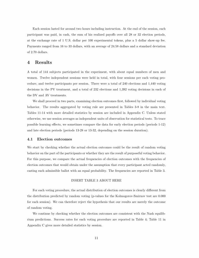
We start by checking whether the actual election outcomes could be the result of random voting

behavior on the part of the participants or whether they are the result of purposeful voting behavior.

For this purpose, we compare the actual frequencies of election outcomes with the frequencies of

election outcomes that would obtain under the assumption that every participant acted randomly,

casting each admissible ballot with an equal probability. The frequencies are reported in Table 3.

INSERT TABLE 3 ABOUT HERE

For each voting procedure, the actual distribution of election outcomes is clearly different from

the distribution predicted by random voting (p-values for the Kolmogorov-Smirnov test are 0.000

for each session). We can therefore reject the hypothesis that our results are merely the outcome

of random voting.

We continue by checking whether the election outcomes are consistent with the Nash equilib-

rium predictions. Success rates for each voting procedure are reported in Table 4; Table 11 in

Appendix C gives more detailed statistics by session.

11

INSERT TABLE 4 ABOUT HERE

We find that under PV, 99.6% of election outcomes are consistent with the outcome of a Nash

equilibrium; the corresponding percentages are 95.7% and 90.5% for AV and DV, respectively.

These numbers are even higher if one considers late election periods. Indeed, under PV 99.3% of

late election outcomes (or 143 out of 144) are consistent with Nash equilibrium predictions, and

under both AV and DV 96.3% of late election outcomes (or 131 out of 136) are consistent with

Nash equilibrium predictions.

The predictive power of Nash equilibrium is still very strong if one restricts attention to Nash

equilibria in weakly undominated voting strategies (WUNE). A ballot is said to be weakly dom-

inated if there exists another ballot that never makes the participant worse off and makes him

sometimes strictly better off.19 As Table 4 further reports, under PV 99.6% of election outcomes

are consistent with the outcome of a Nash equilibrium in weakly undominated voting strategies;

the corresponding percentages are 68.1% and 77.6% for AV and DV, respectively. These numbers

are even higher for late election periods: 99.3% for PV, 75% for AV, and 84.5% for DV.

Conclusion 1 summarizes these results.

Conclusion 1 For each voting procedure the actual distribution of election outcomes is signif-

icantly different from the distribution of election outcomes that corresponds to random voting.

Almost all election outcomes are consistent with (pure-strategy) Nash equilibrium predictions. An

overwhelming majority of election outcomes are also consistent with Nash equilibrium in weakly

undominated (pure) voting strategies. ‖

We now investigate the existence of a two-party system under each of the three voting proce-

dures. In Section 2 above we said that a voting procedure yields a two-party system if in every

equilibrium no more than two candidates are tying for first place. It is obvious that even in a

tightly controlled laboratory experiment it is virtually impossible that it happens in all of the 232

or 240 elections that were conducted under each voting procedure; one would expect to see some

learning and experimentation on the part of participants under any voting rule.

INSERT TABLE 5 ABOUT HERE

Table 5 reports the frequencies of three-way ties under each voting procedure (see also Table 12

in Appendix C). Three-way ties occurred in 0.4% of elections held under PV, in 3% of elections held19Given our design, the following ballots are weakly dominated. Under PV, a ballot is weakly dominated

for a participant if and only if he abstains from voting or votes for his least-preferred candidate. UnderAV, a ballot is weakly dominated for a participant if and only if he abstains from voting, does not vote forall his most-preferred candidates, or casts a vote for his least-preferred candidate. Under DV, a ballot isweakly dominated for a participant if and only if he does not vote for his most-preferred candidate(s).

12

under AV, and in 13.8% of elections held under DV. Thus, three-way ties virtually never happened

in PV elections. Further, the frequency of three-way ties in AV elections is not statistically different

from the frequency of three-way ties in PV elections (p=0.1814 for a Wilcoxon Mann-Whitney rank

order test using session averages as units of observation). By contrast, the frequency of three-way

ties in DV elections is both statistically different from zero and statistically different from the

frequency of three-way ties in PV and AV elections at conventional significance levels (p=0.0286).

Based on these observations we cannot reject the hypothesis that PV and AV yield a two-party

system. At the same time, we can reject the hypothesis that DV yields a two-party system.

These conclusions are even stronger if one takes participants’ learning into account. From

Table 5, we observe no difference between early and late election periods for both PV and AV. In

the case of PV, three-way ties occurred in zero elections out of 96 in the early periods as compared

to one election out of 144 in the late periods. In the case of AV, three-way ties occurred in 3 out

of 96 early elections as compared to 4 out of 136 late elections. By contrast, under DV, three-way

ties occurred much more often in late elections than in early elections: 5.2% or 5 out of 96 early

elections, as compared to 19.9% or 27 out of 136 late elections.

These results are summarized in Conclusion 2.20,21

Conclusion 2 The frequencies of three-way ties in Plurality Voting and Approval Voting elections

are both negligible, and are not statistically different from each other. By contrast, the frequency

of three-way ties in Dual Voting elections is significantly above the frequencies of three-way ties

in Plurality Voting and Approval Voting elections. Thus, we can reject the hypothesis that Dual

Voting yields a two-party system, but we cannot reject the hypothesis that either Plurality Voting

or Approval Voting yields a two-party system. ‖20Because we only re-assigned participants’ positions every four election periods, there is a chance that

we are catching some of the dynamic aspects of the game rather than the equilibrium results from a one-shot game. To help mitigate these elements, we separately looked at the results from the first election ofeach series of four election periods. The above results are even stronger in this context.

21In their experimental test of Duverger’s law Forsythe et al. (1996) use the average difference betweenthe vote totals of the second- and the third-placed candidates. There are several reasons why their test isnot adequate for our purposes. First, Forsythe et al. seek to test the concentration of votes on exactly twocandidates, while our purpose is to test the existence of at most two viable competitors. The second reasonwhy the average second to third place spread is not adequate here is most easily understood in the contextof PV elections. There are (at least) two cases where the spread is equal to zero: (1) a three-way tie; and(2) a unanimous vote for Orange. While the latter case is consistent with PV yielding a two-party system,the former case is not. The third reason why the average second to third place spread is not adequatehere follows from our comparative purposes. By letting or forcing voters to vote for more than one ofthe candidates, the spread is necessarily smaller under Approval and Dual Voting than under PV. Withthe above caveats in mind, we report the vote spreads under each voting procedure. The average secondto third place spread is equal to 31.9% under PV, 16.4% under AV, and 9.2% under DV. Moreover, thespread in each PV session is higher than the spreads in any AV session, and the spread in each AV sessionis higher than the spreads in any DV sessions; the differences in spreads among any two voting proceduresare statistically significant. Based on this test, the support for a two-party system is the strongest underPV, followed in order by AV and DV.

13

So far our results are consistent with the prediction that Plurality and Approval Voting yield a

two-party system in the sense that in each election at most two candidates are tying for first place.

One may wonder however if across elections more than two candidates are viable. In other words,

one may ask whether the same one or two candidates are repeatedly in the winning set (i.e., the

set of candidates who are tying for first place) or whether each of the three candidates is regularly

in the winning set.

INSERT TABLE 6 ABOUT HERE

Table 6 reports, for every voting procedure, the frequency with which each candidate is in the

winning set (see also Table 13 in Appendix C). Orange, the middle candidate, is almost always

in the winning set: in 85.4% of the elections held under PV, 72% of the elections held under AV,

and 86.2% of the elections held under DV. Hence, Orange, the candidate located at 3, appears

focal. Blue, the candidate at 9, is often in the winning set as well – in 39.2%, 50.9% and 30.2%

of the elections held under PV, AV and DV, respectively. By contrast, Green, the candidate at 1,

is (almost) never in the winning set under PV (0.4% of the times), is rarely there under AV (in

only 4.3% of elections), but is frequently in the winning set under DV (in 20.7% of elections).22

The percentage of times Green is in the winning set is significantly higher under DV than under

either PV or AV (p=0.0286 for a Wilcoxon Mann-Whitney test). At the same time, the frequencies

with which Green is in the winning set under PV and under AV are not different at conventional

significance levels (p=0.1814).23 In late periods, Green is even less often in the winning set under

AV (3.7% of late election periods), and more often under DV (25% of late election periods). Thus,

we cannot reject the hypothesis that under both PV and AV only two candidates are viable across

elections. However, we can reject this hypothesis for DV.

These results are summarized in Conclusion 3.

Conclusion 3 Under both Plurality Voting and Approval Voting, only two out of three candidates

are viable across elections: their probability of being in the winning set is strictly positive. By

contrast, under Dual Voting, all three candidates are viable across elections. The middle candidate

is the candidate who is the most frequently in the winning set under all three voting procedures. ‖22Observe that Orange and Blue are both Condorcet winners (i.e., candidates who defeat every other

candidate in a pairwise contest) while Green is a Condorcet loser (i.e., a candidate who is defeated by everyother candidate in a pairwise contest). Thus, the Condorcet loser is almost never elected under Pluralityand Approval Voting, but is regularly in the winning set under DV. However, this feature is design-specificand need not hold in general.

23A matched pairs test using sessions as units of observation shows that Green appears in the winningset less frequently than Blue (p=0.0625 for both PV and AV). This is the best significance level we canget with only four independent observations (sessions) under each voting procedure. In contrast, underDV, the frequencies with which Green and Blue are in the winning set are not statistically different atconventional significance levels (p=0.125).

14

Thus, Conclusion 3 extends across elections the within-election result stated in Conclusion 2.

4.2 Individual voting behavior

In this section, we look at behavioral regularities behind the election outcomes described above.

We start by considering whether the observed multipartism under DV may be attributed to random

factors, or if it is due to strategic voting. We say that a vote is strategic if it is neither sincere nor

weakly dominated; a vote is said to be sincere if whenever the voter votes for a candidate, he also

votes for all the candidates he prefers to that candidate.24

Recall, from Section 2, that in our experimental setting, an equilibrium with a three-way tie

occurs under DV only if the voters located at 10 behave strategically, casting one vote for their

most-preferred candidate, Blue, and dumping their second vote on their least-preferred candidate,

Green. (If, instead, they vote sincerely for the two candidates they most prefer, Blue and Orange,

then Orange wins outright.) By contrast, the same voters have no incentive to cast a vote for

Green if the election is held under PV or AV. Furthermore, casting a vote for Green is weakly

dominated for the voters located at 10 if the election is held under Plurality or Approval Voting.

We now investigate the voting behavior of our participants when they are located at 10.

INSERT TABLE 7 ABOUT HERE

Table 7 reports the frequencies with which each ballot was cast by the participants at 10 (see

also Table 14 in Appendix C).25 There are several things worth pointing out. First, among all

voting decisions made by the participants at 10, only 1.67% (8 out of 480) of the voting decisions

under PV, and only 8.41% (39 out of 464) of the voting decisions under AV, included a vote for

Green. By contrast, under DV, 50.44% of the voting decisions made by the participants in this

position (234 voting decisions out of 464) included a vote for Green. This number is significantly

higher than the numbers obtained under PV and AV. Second, the strategic ballot consisting of

a vote for Green and a vote for Blue was cast 43.97% of the times under DV, whereas the same

ballot was cast only 4.31% of the times under AV. Moreover, under DV, this ballot was cast

much more frequently in late election periods than in early election periods (39.06% of the times

in early periods compared to 47.43% in late periods), whereas under AV the frequency was left24For PV, this means that a voter votes sincerely if he votes for (one of) his most-preferred candidate(s).

For DV, this means that a voter votes sincerely if he votes for the two candidates he prefers. Finally, forAV, this means that a voter votes sincerely if he votes either for his most-preferred candidate, or for thetwo candidates he prefers (or for all three candidates). This definition of sincere voting corresponds to theone proposed by Brams and Fishburn (1978).

25For each voting procedure, Table 7 also indicates which ballots are strategic, and which are weaklydominated. One may notice that none of the ballots are marked as strategic under AV. This is becausewith three voting alternatives, every weakly undominated ballot under AV is sincere (Brams and Fishburn1978, Theorem 3).

15

virtually unchanged (4.17% in early periods compared to 4.41% in late periods). Figure 2 further

demonstrates that in late DV elections many of the participants chose to cast the strategic ballot

each time they were located at 10.

FIGURE 2 ABOUT HERE.

Finally, note that in DV elections the strategic ballot (Green, Blue) was cast more often than

the sincere ballot (Orange, Blue) – 43.97% as compared to 41.38%. This difference is even more

pronounced if one takes participants’ learning into account; the corresponding percentages for

late election periods are 47.43% for the strategic ballot as compared to 38.97% for the sincere

ballot. This observation is quite remarkable since casting the sincere ballot (Orange, Blue) and

casting the strategic ballot (Green, Blue) are both equilibrium strategies for the voters at 10 under

DV; the sincere ballot is part of the Nash equilibrium where Orange wins outright, whereas the

strategic ballot is part of the three-way-tie equilibrium (both equilibria are in weakly undominated

strategies). However, the voters at 10 may prefer the three-way-tie equilibrium because of a higher

expected payoff.

These results are summarized in Conclusion 4.

Conclusion 4 Multipartism in the Dual Voting experimental elections emerged because of strategic

voting behavior on the part of participants. Voters in position 10 voted strategically almost half of

the time, casting one vote for their most-preferred candidate (Blue), and dumping their other vote

on their least-preferred candidate (Green). In contrast, under both Plurality Voting and Approval

Voting, participants at 10 cast very few votes for their least-preferred candidate (Green), yielding

a two-party system. ‖

We next consider how often our participants cast weakly dominated ballots. The casting

of only few weakly dominated ballots would provide evidence of sophistication on the part of

participants and their ability to understand the voting procedure. By contrast, the casting of

many weakly dominated ballots would suggest that the participants did not fully understand the

voting procedure.

INSERT TABLE 8 ABOUT HERE

The frequencies with which weakly dominated ballots were cast are reported in the first three

columns of Table 8. Weakly dominated ballots were rarely cast under PV (only 2.8% of ballots

overall), whereas a significant fraction of the ballots cast under DV (12.5%) and an extremely

high fraction of the ballots cast under AV (36.2%) were weakly dominated. For any two voting

16

procedures, the frequencies with which weakly dominated ballots were cast are statistically different

(p=0.0286 for a Wilcoxon Mann-Whitney test in all cases). Table 8 also shows that the percentage

of elections in which at least one participant cast a weakly dominated ballot was the highest under

AV (93.5% of all elections), followed by DV (54.7% of elections), followed by PV (15.4% of all

elections). Again, the differences between any two voting rules are all significant (p =0.0286).

It is possible that weakly dominated ballots were mostly cast in early elections with the partic-

ipants learning not to cast weakly dominated ballots as the sessions progressed. Table 8 indicates

that some learning seem to have taken place under DV; the share of weakly dominated ballots cast

under DV dropped from 15.1% in early election periods to 10.7% in late periods. By contrast,

the share of weakly dominated ballots under both PV and AV remained rather stable: under PV,

3.5% in early election periods as compared to 2.4% in late periods; and under AV, 36.5% in early

election periods as compared to 36% in late periods.

We further checked for the presence of learning by testing for each voting procedure and for

each voter position, whether the election period was a good predictor of the likelihood that a

weakly dominated ballot was cast. We found that DV was the only voting rule among the three

studied here where the likelihood of casting a weakly dominated ballot decreased significantly as

periods progressed. For the other two voting rules, the election period was not a good predictor

of the likelihood with which a weakly dominated ballot was cast.

Conclusion 5 summarizes the above observations.

Conclusion 5 Among the three voting procedures, Plurality Voting had the smallest share of

weakly dominated ballots, followed in order by Dual Voting and Approval Voting. Under Plu-

rality Voting, weakly dominated ballots were rarely cast, whereas under Approval Voting every third

ballot cast was weakly dominated. Under Approval Voting there was little learning on the part of

the participants to avoid casting weakly dominated ballots. By contrast, some learning took place

under Dual Voting. ‖

The widespread and persistent use of dominated strategies by experimental subjects under

AV but not under PV is consistent with Rapoport et al.’s (1991) findings, who attribute this

phenomenon, in part, to the novelty and complexity of AV as compared to PV. If we use the

frequency of weakly dominated ballots cast as an empirical measure of a voting rule complexity,

then, based on our data, PV appears the simplest, and AV appears the most complex, among the

three voting procedures that we study.

Finally, we look at subject heterogeneity among participants.

INSERT FIGURE 3 ABOUT HERE.

17

Figure 3 illustrates the distribution of weakly dominated ballots among participants. While many

participants rarely cast weakly dominated ballots, a few did cast weakly dominated ballots almost

every period. We reject the hypothesis that there was no individual heterogeneity using the

Kolmogorov-Smirnov one-sample test under all three voting rules (p-value = .000). A similar

result applies with regards to the casting of the strategic ballot in DV elections; see Figure 2,

above. Some participants were systematically casting the strategic ballot each time they were

located at position 10, starting early on in the session. By contrast, others chose never to cast the

strategic ballot. Again, these differences are highly significant (p-value = .000). We conclude:

Conclusion 6 Participants were heterogeneous both in their propensity to cast weakly dominated

ballots and in their propensity to cast the strategic ballot under Dual Voting. ‖

Interestingly, we observe that individuals casting weakly dominated ballots did not always

affect aggregate voting outcomes. Weakly dominated votes were cast by individual voters in many

elections (see Table 8); yet, most of the election outcomes were consistent with the outcome of

a Nash equilibrium in weakly undominated strategies (Conclusion 1 in Section 4.1 above). The

starkest example is AV, where 93.5% of (or 217 out of 232) elections included at least one weakly

dominated ballot, but 68.1% of electoral outcomes (or 158 out of 232) were still consistent with

Nash equilibria in weakly undominated strategies (Tables 4 and 8). This suggests that in aggregate,

people’s ‘mistakes’ largely canceled each other out, thereby yielding the same outcomes as if all

the ballots cast were weakly undominated.26 In contrast to “mistakes”, participants’ purposeful

(strategic) behavior often did have an effect on electoral outcomes: many outcomes under DV

corresponded to the Nash equilibrium under strategic voting (Conclusions 2 and 4).

4.3 Bounded Rationality

We now consider whether models of bounded rationality may add to explaining the participant

behavior in our experiment. We consider two popular models: Quantal Response Equilibrium and

level-k reasoning.

Quantal Response Equilibrium (QRE) is a model of bounded rationality first developed by

McKelvey and Palfrey (1995). In QRE, subjects’ beliefs of their expected payoffs, while correct on26The experimental evidence that outcomes of many institutions, especially markets, are robust to in-

dividual errors, has been used by experimental economists to justify the rationality approach to socialsciences. Charles Plott writes: “Claims about the irrelevance of models of rational choice and the con-sequent irrelevance of economics are not uncommon... If one looks at experimental markets for evidence,the pessimism is not justified. Market models based on rational choice principles... do a pretty good jobof capturing the essence of very complicated phenomena” (1986, p. S325). Colin Camerer also notes that“... better models of individual decision making may not improve market level predictions; whether theydo so is fundamentally an empirical question that economic experiments help answer...” (Camerer, 1995,p. 589).

18

average, are subject to random error. In the most common form of QRE, logit QRE, the stochastic

error term is assumed to be drawn from a logit distribution. Because the error term can be any

real number, all strategies are chosen with positive probability, but strategies with higher true

expected payoff are played with higher frequency than strategies with lower expected payoffs.27 Of

particular importance in the QRE model, is the parameter λ, which is inversely proportional to

the spread of the stochastic error term. When the subjects’ expected payoffs are subject to very

large error terms, (i.e., λ is very low), subjects tend to randomize more with λ → 0 converging

to perfectly random strategy mixing. Conversely, as λ → ∞, subjects’ plays converge to a Nash

equilibrium. The predicted probabilities for select strategies given different levels of λ are expressed

in Figures 5 - 7 in Appendix D.28

Two observations regarding the QRE predictions are of particular interest for our experimental

results. First, even as the error term decreases to zero (i.e., λ → ∞), the limit strategies for QRE

equilibrium still contain weakly dominated strategies. This further suggests that assuming subjects

do not cast weakly dominated ballots may be an overly restrictive assumption. Second, under Dual

Voting, for voters in position 10 the only strategy that is consistent with the QRE limiting strategy

is the strategic vote (Green, Blue).29 Thus, the limit of the QRE model as λ → ∞ predicts that,

under Dual Voting, participants in position 10 should always vote strategically.

The maximum likelihood estimations for λ for each of the three voting rules, along with the

corresponding QRE predictions on different types of strategies used, are summarized in Table 9,

below.30

INSERT TABLE 9 ABOUT HERE

The QRE estimations make some correct qualitative predictions about the data. In general, as

per QRE predictions, subjects did cast many weakly dominated ballots, but they tended to cast

higher expected payoff ballots more frequently than low expected payoff ballots. For example, a27Specifically, the probability player i plays strategy sij ∈ Si, denoted σi (sij) is given by σi(sij) =

eλEPi(sij)

∑sik∈Si

eλEP (sik) , where EP (sij) is the equilibrium expected payoff from choosing strategy sij .28To our knowledge, Figure 7 features the first publicized game where the primary QRE branch contains

a backward bending section. Many thanks to Ted Turocy for his insight into QRE and for helping us verifythe stability of the ‘forward-moving’ branches.

29The following Nash equilibrium strategies are the limit strategies for QRE equilibrium, as λ approachesinfinity: For PV, voters at 2 vote for Orange; voters at 9 vote for Blue; and voters at 6 vote for Orange, orBlue or abstain; thus Orange or Blue may win. For AV, voters at 2 vote for Orange, or Green and Orange;voters at 6 vote for Orange, or Blue, or Orange and Blue; and voters at 10 vote for Blue; thus Orange orBlue may win. For DV, voters at 2 vote for Green and Orange; voters at 6 vote for Orange and Blue; andvoters at 9 vote for Green and Blue; thus a three-way tie occurs, and Green or Orange or Blue may win.

30The table reports the frequencies of sincere, weakly dominated, and, when applicable, strategic ballots.The QRE predicted frequencies of weakly dominated ballots are especially high for the participants inposition six. This is because the payoffs for each of the three candidates winning are very similar, makingplayers in position six largely indifferent between all their available strategies.

19

substantial number of subjects in position 2 under AV (23.3%) cast ballots only for their preferred

alternative that had a reasonable chance of being in the winning set (Orange), despite the fact

that voting for both Orange and Green weakly dominated it. QRE also provides us with another

indication that there was little to no learning under either PV or AV, but that there was substan-

tial learning under DV.31 However, QRE drastically overpredicts the number of weakly dominated

ballots cast. This suggests that while our subjects may not have been rational enough to exclu-

sively cast weakly undominated ballots, they were sophisticated enough to do it fairly often. One

possible reason why QRE may have produced substantial estimation errors is because the baseline

QRE model assumes that all subjects are homogeneous.32 Since our experimental participants

were highly heterogeneous both in their propensity to cast weakly dominated ballots as well as

their propensity to vote strategically (Conclusion 6, above), we next turn to a model of bounded

rationality that can take subject differences into consideration.

Starting with Nagel (1995), many studies have attempted to explain subjects’ choices based

on the ‘depth of reasoning’ made for their experimental choices. Following Costa-Gomez and

Crawford (2006), level-k reasoning model categorizes subjects into different types or ‘levels’. A

level 0 subject is one that perfectly randomizes among all available alternatives. A level k subject,

meanwhile, assumes that all other subjects are level (k−1) and best respond most of the time, but

randomize their play with some finite probability. This randomization is assumed known by all

higher-level players. While not all players follow this typing exactly, the above papers and other

suggest that a large fraction of subjects do. Thus, it is not necessary to try to assign types to all of

our subjects, but instead we simply note the implications of having a large fraction of our subjects

be level-k reasoners. Table 10, below, summarizes the preferred ballots of level-k subjects. Note

that under all voting rules and for all positions, the preferred ballots for all subjects level 2 and

above are identical. Thus the table only reports on levels 1 and 2.

TABLE 10 ABOUT HERE.

One particularly appealing aspect of using level-k reasoning for this experiment is that it

gives a clear explanation for why some subjects cast predominantly sincere ballots while others31This is done by estimating λ separately for early and late periods under each voting rule. To the

extent that QRE’s λ parameter measures the degree of randomness of subjects’ voting, a higher λ couldbe correlated with a higher degree of sophistication. Although MLE λ values increased from early to lateperiods under both PV and AV (from .120 to .133 and from .128 to .130 respectively), the increase wasmuch more pronounced under DV where it increased from .185 to .321.

32Camerer et al. (2008) provide a framework for a heterogeneous QRE model that also encompasses thelevel-k reasoning model presented below. However, just as regular QRE requires parametric assumptionsto provide explanatory power (see Haile et al. 2008), so too does a heterogeneous QRE model. Here weuse a more computationally developed homogeneous QRE model.

20

cast predominantly strategic ballots when in the strategic position under DV. Specifically, level-

1 subjects cast sincere ballots because they fear Green winning outright, while level-2 subjects

cast strategic ballots because they believe that Orange will win outright otherwise. Furthermore,

unlike QRE, level-k reasoning is able to correctly predict the large frequency of weakly undominated

ballots under AV.

However, there are several drawbacks to using level-k reasoning to analyze the current data.

Aside from the theoretical issues with using it for repeated games, the limited strategy space of

this game makes it very difficult to distinguish between types, especially under AV where all types

have the same preferred ballot for each position. Further, level-k reasoning predicts a large number

of votes cast for Blue under PV, something that is not observed empirically.33 Instead, all sessions

had a very strong centrist effect, where the central candidate (Orange) received a lion’s share of

the votes.

Conclusion 7, below, summarizes our findings on the above two models of bounded rationality.

Conclusion 7 Quantal Response Equilibrium correctly predicts that voters tend to cast higher

expected payoff ballots more frequently than low expected payoff ballots, and that voters under Dual

Voting often vote strategically. At the same time, QRE drastically overpredicts the shares of weakly

dominated ballots cast. Level-k reasoning allows to explain a degree of observed subject heterogeneity

as well as a large share of weakly undominated ballots. At the same time, it fails to predict the

prevalence of ballots cast for the centrist candidate under Plurality Voting. ‖

5 Discussion and conclusion

Duverger’s law states that countries where policymakers are elected under Plurality Voting tend

to have a two-party system. This empirical regularity has been explained by the wasting-the-vote

effect of Plurality Voting: fearing to waste their vote on an underdog, voters are led to behave

strategically and vote for the serious contender they prefer (instead of voting sincerely for the

contender they most prefer). Such strategic behavior on the part of voters triggers a desertion

of the trailing candidates and a concentration of the votes on only two candidates. Dellis (2007)

shows that this Duvergerian logic generalizes to some voting procedures other than Plurality Voting.

Approval Voting, in particular, is predicted to yield a two-party system as well. The key feature of

Approval Voting that allows to sustain the two-party system is admissibility of truncated ballots:

voters are allowed, but not forced to vote for multiple candidates. Forcing the voters to vote for33Specifically, level-1 subjects in position 6 are indifferent between voting for Orange and Blue, and are

generally assumed to randomize between the two. Level-2 subjects and higher, meanwhile, exclusively votefor Blue. Therefore, if any subjects are level-2 or higher, then we should expect a larger share of subjectscasting ballots for Blue. Most studies predict at least 50% of subjects are level-2 or above.

21

more than one candidate, as under Dual Voting, may generate incentives for strategic vote dumping

that may give rise to multipartism.

Our experimental results provide evidence that is in line with the above predictions. In the

overwhelming majority of our Plurality Voting and Approval Voting elections, either one candidate

won the election outright, or two candidates tied for first place. In contrast, the Dual Voting

elections often resulted in three-way ties among the candidates, due to strategic voting in the form

of vote dumping by certain voters. We thus provide evidence that voters’ ability to truncate ballots

is essential for maintaining the two-party system under Approval Voting.

Our results help ease fears raised by many scholars – including the supporters of Approval

Voting – that using Approval Voting for (U.S.) political elections would obliterate the two-party

system. This fear was best captured by Cox (1997; 95) when he wrote: “... many believe that

[Approval Voting] would lead to multipartism, although there is no empirical evidence on this

score.” Notice that the emergence of a two-party system under Approval Voting is here the more

remarkable that our participants were unfamiliar with Approval Voting and that no education

effort had been undertaken prior the experiment.

We also observe some features of the individual voting behavior that have implications for

the implementability of Approval Voting and Dual Voting. One reasonable (and rather minimal)

requirement for a voting procedure to be implementable is that people understand it well enough

that they do not cast weakly dominated ballots. Our results suggest that contrary to Plurality

Voting, neither Approval Voting nor Dual Voting meet this requirement, even in a setting as simple

as in our experiment. Even more troublesome for Approval Voting is that people may not learn

over time to avoid casting weakly dominated ballots. This raises doubts on the claim made by the

supporters of Approval Voting that Approval Voting is simple for voters to understand. Despite

this conclusion, there is some hope that the problem would not be that serious if Approval Voting

was used for political elections. Indeed, party elites and media – two actors that are absent from

our experiment – may undertake an education effort toward the citizens. Also, political parties

may make suggestions to their supporters on how to vote in the election.34 If political parties

and interest groups guide the voters, then strategic voting behavior that was observed in our small

experimental elections may, under certain circumstances, also be encouraged and observed in larger

scale elections.34This is done for example in Australia, where legislative elections are held under Single Transferable

Vote (a voting rule which is much more complex than any of those we have considered here). In LowerHouse elections, it takes the form of voting cards that parties distribute to voters when they enter thepolling station and that suggest voters a specific ballot to cast. In Senate elections, it takes the form ofpolitical parties submitting beforehand a ballot and voters having the option to tick a box on the ballotpaper to select the ballot submitted by that party. For more details on the Australian electoral systemand the coordination role by political parties, see chapters 3 and 6 in Farrell (2001).

22

Another implication of our results concerns the usefulness of the weak undominance refinement

in the theoretical voting literature. If people are frequently casting weakly dominated ballots (as

was the case here in Approval Voting elections and, to a lesser extent, in Dual Voting elections),

then restricting attention to equilibria in weakly undominated voting strategies may yield mislead-

ing predictions. Moreover, if the frequency of weakly dominated ballots varies from one voting

procedure to another (as we have observed here), one may question the desirability of using this

refinement for comparing alternative voting procedures – a standard practice in the formal voting

literature. It is important to note, however, that despite the prevalence of participants casting

weakly dominated ballots under both Approval Voting and Dual Voting, most of our experimen-

tal elections delivered an outcome that was consistent with the outcome of a Nash equilibrium

in weakly undominated voting strategies. This suggests that in aggregate people ‘mistakes’ may

cancel each other out, thereby yielding the same electoral outcomes as if all the ballots cast were

weakly undominated.

As a word of caution, we emphasize that we see our results as preliminary evidence on the

effect of the three voting rules on the two-party system. Many robustness checks with varying

numbers and locations of voters and candidates are needed. Further, to make the setting more

realistic, it is important to incorporate strategic candidacy decisions into the analysis. Another

issue to consider is that of path dependence in electoral reforms. The current experiment shows

that multipartism may arise under Dual Voting, but it is silent about whether multipartism is

likely to occur following an electoral reform where Plurality Voting is replaced with Dual Voting.

More generally, in the presence of multiple equilibria – as is the case in our setting – we would

like to know which of them will become focal following the replacement of Plurality Voting with

another voting procedure. Our present evidence indicates that an equilibrium with the middle

candidate in the winning set might be focal. We are currently working on these questions.

23

Appendix A: Experimental Instructions

Experimental Instructions (PV)

Introduction

You are about to participate in an experiment in the economics of decision making in which you

will earn money based on the decisions you make. All earnings you make are yours to keep and will

be paid to you IN CASH at the end of the experiment. During the experiment all units of account

will be in experimental dollars. Upon concluding the experiment the amount of experimental

dollars you earn will be converted into dollars at the conversion rate of 1 U.S. dollar per 100

experimental dollars. Your earnings plus a lump sum amount of 5 U.S. dollars will be paid to

you in private.

Do not communicate with the other participants except according to the specific rules of the

experiment. If you have a question, feel free to raise your hand. An experimenter will come over

to you and answer your question in private.

In this experiment you are going to participate in a decision process along with 11 other

participants. From now on, you will be referred to by your ID number. Your ID number will be

assigned to you by the computer.

Periods and Groups

Decisions in this experiments will occur in a sequence of independent decision periods. At the

beginning of the the first decision period, you will be assigned to a decision group with 5 other

participant(s). You will not be told which of the other participants are in your decision group.

What happens in your group has no effect on the participants in other groups and vice versa. The

group composition will stay the same for 4 periods, but will change afterwards.

Decisions and Outcomes

During each period, you will be asked to choose, or vote for, one of the three alternatives, Green,

Orange, and Blue. All participants in your group will make their decisions at the same time,

without knowing the choices of others. The computer will then select as an outcome for your group

the alternative that most of the participants in your group voted for. If two or more alternatives

get the same highest number of votes, then an alternative among those with the highest number

of votes will be selected as an outcome randomly.

Example 1 Suppose the number of votes for each alternative in your group are: 1 vote for

Green, 2 votes for Orange, and 3 votes for Blue, then Blue will be the outcome for your group.

24

Example 2 Now suppose there are 3 votes for Green, 3 votes for Orange, and 0 votes for Blue.

Then the outcome will be chosen randomly between Green and Orange.

Voting Rules

In each period, you will be asked to choose (vote for) EXACTLY ONE of the alternatives. You

may also choose to vote for NONE, but if you decide to vote for any, then you must vote for exactly

one. The voting rule will stay the same for the whole experiment.

Payoffs

The value of decisions to you (your payoffs from each alternative) will be given to you by the

computer before you make your choices. (You will also know the payoffs of other participants in

your group before you make your decisions.) In order to understand how your payoffs depend on

the alternative chosen, suppose that the alternatives have positions on a number line, and you (as

well as other participants in your group) have your most preferred, or ideal position, on this line.

For example, the picture below indicates that Orange, Green and Blue correspond to positions 3,

6, and 9, respectively. The participant’s ideal positions, or locations, are marked with ”X” on the

graph, with your ideal position highlighted in red.

For example, on this picture your ideal position is at 5. The picture indicates that there is

another participant located at the same position, two other participants are located at 8, and the

other two participants are located at 10.

The amount of payoff you receive in a given period depends on how close the selected alterna-

tive, or the outcome for the period, is to your ideal position. The closer the outcome is to your

ideal position, the higher is your payoff. For example, the picture above indicates that Green and

Orange are closer to your position than Blue, and therefore they will correspond to a higher payoff

for you than Blue.

25

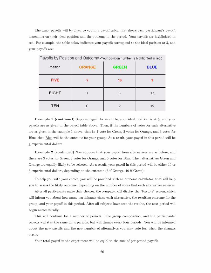
The exact payoffs will be given to you in a payoff table, that shows each participant’s payoff,

depending on their ideal position and the outcome in the period. Your payoffs are highlighted in

red. For example, the table below indicates your payoffs correspond to the ideal position at 5, and

your payoffs are:

Example 1 (continued) Suppose, again for example, your ideal position is at 5, and your

payoffs are as given in the payoff table above. Then, if the numbers of votes for each alternative

are as given in the example 1 above, that is: 1 vote for Green, 2 votes for Orange, and 3 votes for

Blue, then Blue will be the outcome for your group. As a result, your payoff in this period will be

1 experimental dollars.

Example 2 (continued) Now suppose that your payoff from alternatives are as before, and

there are 3 votes for Green, 3 votes for Orange, and 0 votes for Blue. Then alternatives Green and

Orange are equally likely to be selected. As a result, your payoff in this period will be either 10 or

5 experimental dollars, depending on the outcome (5 if Orange, 10 if Green).

To help you with your choice, you will be provided with an outcome calculator, that will help

you to assess the likely outcome, depending on the number of votes that each alternative receives.

After all participants make their choices, the computer will display the “Results” screen, which

will inform you about how many participants chose each alternative, the resulting outcome for the

group, and your payoff in this period. After all subjects have seen the results, the next period will

begin automatically.

This will continue for a number of periods. The group composition, and the participants’

payoffs will stay the same for 4 periods, but will change every four periods. You will be informed

about the new payoffs and the new number of alternatives you may vote for, when the changes

occur.

Your total payoff in the experiment will be equal to the sum of per period payoffs.

26

The first two periods in the experiment will be trial periods. They will not count toward your

earnings.

ARE THERE ANY QUESTIONS?

If you have a question during the experiment, please raise your hand and I will come by to

answer your question.

Exercises

Exercise 1 Suppose that your payoff from Green is 11, your payoff from Orange is 13, and your

payoff from Blue is 8 experimental dollars. Given the choices of the participants listed below, fill

in the alternative(s) that may selected and your corresponding payoff(s):

Number of votes for Green: 5

Number of votes for Orange: 4

Number of votes for Blue: 2

Can Green be selected? 2 yes 2 no

Can Orange be selected? 2 yes 2 no

Can Blue be selected? 2 yes 2 no

Your payoff will be:

Exercise 2 Now suppose the numbers of votes for each alternative are as listed below. Fill in

the alternative(s) that may selected and your corresponding payoff(s) for this period (assume that

your payoffs are the same as in Exercise 1 above):

Number of votes for Green: 4

Number of votes for Orange: 4

Number of votes for Blue: 4

Can Green be selected? 2 yes 2 no

Can Orange be selected? 2 yes 2 no

Can Blue be selected? 2 yes 2 no

Your payoff will be:

ARE THERE ANY QUESTIONS?

27

Appendix B: Subject Computer Screenshot

FIGURE 4 HERE

Appendix C: Additional Tables

TABLES 11-14 HERE

Appendix D: Additional Figures

FIGURES 5 - 7 HERE

28

References

[1] Battaglini, M., Morton, R., Palfrey, T., 2007. Efficiency, equity, and timing of voting mecha-

nisms. American Political Science Review 101, 409-424.

[2] Blais, A., Laslier, J-F., Sauger, N., Van der Straeten, K., 2008. Sincere, Strategic, and Heuris-

tic Voting under Four Election Rules: An Experimental Study. Mimeo.

[3] Brams, S., 2007. Mathematics and Democracy. Princeton University Press, Princeton, NJ.

[4] Brams, S., Fishburn, P., 1978. Approval voting. American Political Science Review 72, 831-

847.

[5] Callander, S., 2005. Electoral competition in heterogeneous districts. Journal of Political Econ-

omy 113, 1116-1145.

[6] Camerer, C., 1995. Individual decision making. In: Handbook of Experimental Economics, J.

Kagel and A. Roth (eds), Princeton University Press, Princeton, NJ, 587-704.

[7] Camerer, C., Palfrey, T., Rogers, B., 2008. Heterogeneous Quantal Response Equilibrium and

Cognitive Hierarchies. Mimeo.

[8] Collier, K., McKelvey, R., Ordeshook, P., Williams, K., 1987. Retrospective voting: An ex-

perimental study. Public Choice 53, 101- 30.

[9] Costa-Gomez, M., Crawford, V., 2006. Cognition and behavior in two person guessing games:

an experimental study. American Economic Review 96, 1737-1768.

[10] Cox, G., 1987. Electoral equilibrium under alternative voting institutions. American Journal

of Political Science 31, 82-108.

[11] Cox, G., 1990. Centripetal and centrifugal incentives in electoral systems. American Journal

of Political Science 34, 903-935.

[12] Cox, G., 1997. Making Votes Count. Cambridge University Press, Cambridge.

[13] Dellis, A., 2007. The Two-Party System under Alternative Voting Procedures. Mimeo.

[14] Duverger, M., 1954. Political Parties. Wiley, New York, NY.

[15] Farrell, D., 2001. Electoral Systems. A Comparative Introduction. Palgrave, New York, NY.

[16] Feddersen, T., 1992. A voting model implying Duverger’s law and positive turnout. American

Journal of Political Science 36, 938-962.

[17] Fey, M., 1997. Stability and coordination in Duverger’s law: A formal model of preelection

polls and strategic voting. American Political Science Review 91, 135-147.

29

[18] Fey, M., 2007. Duverger’s Law without Strategic Voting. Mimeo.

[19] Fischbacher, U., 2007. z-Tree: Zurich Toolbox for Ready-made Economic Experiments. Ex-

perimental Economics 10, 171-178.

[20] Forsythe, R., Myerson, R., Rietz, T., Weber, R., 1993. An experiment on coordination in

multi-candidate elections: The importance of polls and election histories. Social Choice and

Welfare 10, 223-247.

[21] Forsythe, R., Rietz, T., Myerson, R., Weber, R., 1996. An experimental study of voting rules

and polls in three-candidate elections. International Journal of Game Theory 25, 355-383.

[22] Haile, P., Hortacsu, A., Kosenok, G., 2008. On the emprical value of Quantal Response

Equilibrium. American Economic Review 98, 180-200.

[23] Hinich, M., Munger, M., 1994. Ideology and the Theory of Political Choice. The University of

Michigan Press, Ann Arbor, MI.

[24] Hirano, S., Snyder, J., 2007. The decline of third party voting in the United States. Journal

of Politics 69, 1-16.

[25] Laslier, J-F., Van Der Straeten, K., 2008. A live experiment on approval voting. Experimental

Economics 11, 97-105.

[26] Lizzeri, A., Persico, N., 2001. The provision of public goods under alternative electoral incen-

tives. American Economic Review 91, 225-239.

[27] Lizzeri, A., Persico, N., 2005. A drawback of electoral competition. Journal of the European

Economic Association 3, 1318-1348.

[28] McKelvey, R., Palfrey, T., 1995. Quantal response equilibria for normal form games. Games

and Economic Behavior 10, 6-38.

[29] Morelli, M., 2004. Party formation and policy outcomes under different electoral systems.

Review of Economic Studies 71, 829-853.

[30] Morton, R., Williams K., 1999. Information asymmetries and simultaneous versus sequential

voting. American Political Science Review 93, 51-67.

[31] Myatt, D., 2007. On the theory of strategic voting. Review of Economic Studies 74, 255-281.

[32] Myerson, R., 2002. Comparison of scoring rules in Poisson voting games. Journal of Economic

Theory 103, 219-251.

30

[33] Myerson, R., Weber, R., 1993. A theory of voting equilibria. American Political Science Review

87, 102-114.

[34] Nagel, R., 1995. Unravelling in guessing games: an experimental study. American Economic

Review 85, 1313-1326.

[35] Palfrey, T., 1984. Spatial equilibrium with entry. Review of Economic Studies 51, 139-156.

[36] Palfrey, T., 1989. A mathematical proof of Duverger’s law. In: Models of Strategic Choice in

Politics, P. Ordeshook (ed.), University of Michigan Press, Ann Arbor, MI.

[37] Palfrey, T., 2006. Laboratory experiments. In: The Oxford Handbook of Political Economy,

B. Weingast and D. Wittman (eds), Oxford University Press, Oxford, 915-936.

[38] Persson, T., Tabellini, G., 2003. The Economic Effects of Constitutions. MIT Press, Cam-

bridge, MA.

[39] Plott, C., 1986. Rational choice in experimental markets. Journal of Business 59, S301-S327.

[40] Poole, K., Rosenthal, H., 1991. Patterns of congressional voting. American Journal of Political

Science 35, 228-278.

[41] Rapoport, A., Felsenthal, D., Maoz, Z., 1991. Sincere versus strategic voting behavior in

small groups. In: Laboratory Research in Political Economy, T. Palfrey (ed.), The University

of Michigan Press, Ann Arbor, MI, 201-235.

[42] Rietz, T., 2003. Three-Way Experimental Election Results: Strategic Voting, Coordinated

Outcomes and Duverger’s Law. Mimeo.

[43] Rietz, T., Myerson, R., Weber, R., 1998. Campaign finance levels as coordinating signals in

three-way, experimental elections. Economics and Politics 10, 185-217.

[44] Riker, W., 1982. The two-party system and Duverger’s law: An essay on the history of political

science. American Political Science Review 76, 753-766.

[45] Roubini, N., Sachs, J., 1989. Political and economic determinants of budget deficits in the

industrial democracies. European Economic Review 33, 903-938.

[46] Weber, S., 1992. On hierarchical spatial competition. Review of Economic Studies 59, 407-425.

[47] Weber, S., 1998. Entry deterrence in electoral spatial competition. Social Choice and Welfare

15, 31-56.

31

List of Tables

1. Experimental Design: Payoff Matrix

2. Equilibria

3. Frequency of Outcomes, by Voting Rule and Session

4. Nash and Weak Undominance Nash Equilibrium Outcomes by Voting Rule

5. Share of Three-Way Ties in Election Outcomes

6. Frequencies of Each Alternative Appearing in the Winning Set, by Voting Rule

7. Ballots Cast by Participants in Position 10, percent

8. Weakly Dominated Votes

9. Actual and Predicted Frequencies Under Quantal Response Equilibrium, by Position and

Voting Rule

10. Preferred Ballots Under Level-k Reasoning

11. Nash and Weak Undominance Nash Equilibria, by Voting Rule and Session

12. Share of Three-Way Ties in Election Outcomes, by Session

13. Frequencies of Each Alternative Appearing in the Winning Set, by Session

14. Ballots Cast by Participants in Position 10, by Session, percent

List of Figures

1. Experimental Design: Number Line Representation

2. Distribution of Strategic Votes among Voters in Position 10 Under Dual Voting

3. Distribution of Weakly Dominated Votes among Voters, by Voting Rule

4. Subject Computer Screenshot

5. Plurality Voting: QRE Predicted Strategies’ Frequencies vs. Observed Frequencies

6. Approval Voting: QRE Predicted Strategies’ Frequencies vs. Observed Frequencies

7. Dual Voting: QRE Predicted Strategies’ Frequencies vs. Observed Frequencies

32

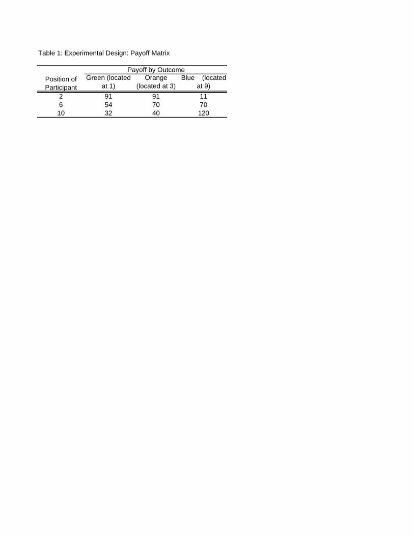
Table 1: Experimental Design: Payoff Matrix

Position of Participant

Payoff by OutcomeGreen (located

at 1)Orange

(located at 3)Blue (located

at 9)2 91 91 116 54 70 7010 32 40 120

Table 2: Equilibria

Voting Rule Equilibrium Outcome Supporting Strategy Profiles**PV {G} All weakly dominated***

{O}* {G,G,O,O,O,O}{G,O,O,O,O,O}{G,O,O,O,O,B}{G,O,O,B,O,O}{G,O,O,O,B,B}{O,O,O,O,O,O}{O,O,O,O,O,B}{O,O,O,B,O,O}{O,O,O,O,B,B}

{B}* {G,G,O,B,B,B}{G,G,B,B,O,B}{G,G,B,B,B,B}{G,O,B,B,B,B}{O,O,B,B,B,B}

{O,B}* {O,O,O,B,B,B}

AV {G} All weakly dominated***{O}* {(G,O),(G,O),(O,B),(O,B),(O,B),(O,B)}{B} All weakly dominated***{O,B}* {(G,O),(G,O),(O,B),(O,B),B,B}

DV {G} All weakly dominated***{O}* {(G,O),(G,O),(O,B),(O,B),(O,B),(O,B)}{B} All weakly dominated***{G,O,B}* {(G,O),(G,O),(O,B),(O,B),(G,B),(G,B)}

The colored alternatives are located at: (G)reen -- 1, (O)range -- 3, (B)lue -- 9

* Indicates the outcome is a WUNE (Nash Equilibrium in Weakly Undomainted Strategies).** Only those not containing weakly dominated strategies are listed. The first two entries list the ballot cast by the participants in position 2, the second two by those in position 6, and the last two by those in position 10.*** All supporting strategy profiles include weakly dominated strategies

Table 3: Frequency of Outcomes, by Voting Rule and Session

Session Green Orange Blue Green and Orange Green and Blue Orange and Blue Three-way tiePV-random 0.24 0.24 0.24 0.08 0.08 0.08 0.05PV-actual -- all 0.00* 0.61** 0.15** 0.00 0.00 0.24** 0.00PV1 0.00 0.73 0.03 0.00 0.00 0.23 0.00PV2 0.00 0.53 0.28 0.00 0.00 0.19 0.00PV3 0.00 0.52 0.16 0.00 0.00 0.30 0.02PV4 0.00 0.64 0.11 0.00 0.00 0.25 0.00

AV-random 0.23 0.23 0.23 0.08 0.08 0.08 0.06AV-actual -- all 0.00* 0.48** 0.28* 0.01 0.00 0.20** 0.03AV1 0.00 0.64 0.22 0.00 0.00 0.14 0.00AV2 0.00 0.43 0.23 0.02 0.00 0.29 0.04AV3 0.00 0.50 0.25 0.00 0.02 0.18 0.05AV4 0.00 0.34 0.41 0.02 0.00 0.20 0.04

DV-random 0.22 0.22 0.22 0.10 0.10 0.10 0.05DV-actual -- all 0.04* 0.64** 0.09* 0.02 0.01 0.07 0.14**DV1 0.02 0.53 0.14 0.00 0.02 0.09 0.20DV2 0.05 0.59 0.09 0.05 0.00 0.07 0.14DV3 0.04 0.80 0.04 0.00 0.00 0.00 0.13DV4 0.07 0.64 0.07 0.02 0.02 0.11 0.07The rows that are marked "-random" show the frequency of each outcome if participants voted randomly.The colored alternatives are located at: Green -- 1, Orange -- 3, Blue -- 9* Consistent with Nash Equilibrium outcome** Consistent with WUNE (Nash Equilibrium in Weakly Undomainted Strategies) outcome

Table 4: Nash and Weak Undominance Nash Equilibrium Outcomes by Voting Rule

NE Outcomes, share WUNE Outcomes, shareall early late all early late

PV 0.996 1.000 0.993 0.996 1.000 0.993(0.004) (0.000) (0.007) (0.004) (0.000) (0.069)

AV 0.957 0.948 0.963 0.681 0.583 0.750(0.013) (0.023) (0.016) (0.031) (0.050) (0.037)

DV 0.905 0.823 0.963 0.776 0.677 0.846(0.019) (0.045) (0.016) (0.027) (0.048) (0.031)

Numbers in parenthesis are the standard errors

Table 5: Share of Three Way Ties in Election Outcomes

Three-way ties, shareall early late

PV 0.004 0.000 0.007(0.004) (0.000) (0.007)

AV 0.030 0.031 0.029(0.011) (0.018) (0.014)

DV 0.138 0.052 0.199(0.023) (0.023) (0.034)

Numbers in parenthesis are the standard errors

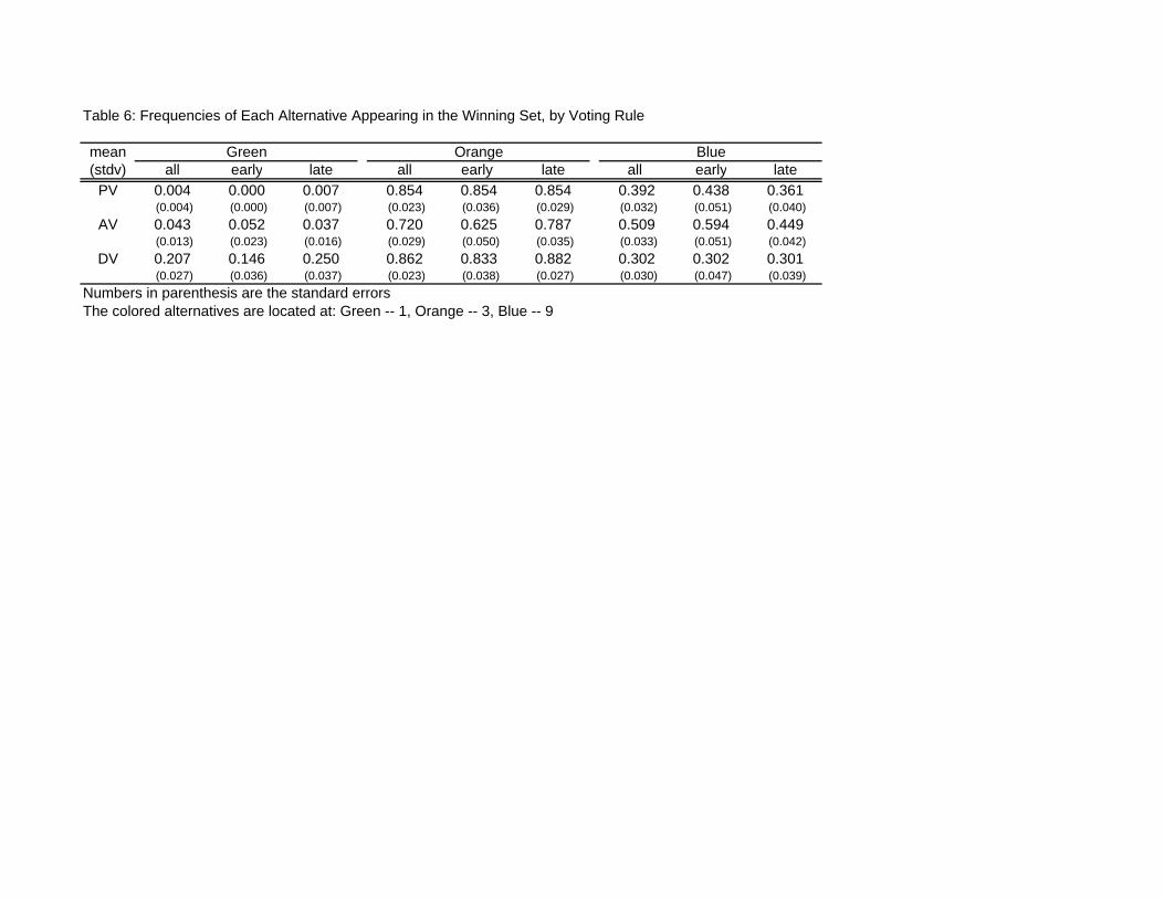
Table 6: Frequencies of Each Alternative Appearing in the Winning Set, by Voting Rule

mean Green Orange Blue(stdv) all early late all early late all early late

PV 0.004 0.000 0.007 0.854 0.854 0.854 0.392 0.438 0.361(0.004) (0.000) (0.007) (0.023) (0.036) (0.029) (0.032) (0.051) (0.040)

AV 0.043 0.052 0.037 0.720 0.625 0.787 0.509 0.594 0.449(0.013) (0.023) (0.016) (0.029) (0.050) (0.035) (0.033) (0.051) (0.042)

DV 0.207 0.146 0.250 0.862 0.833 0.882 0.302 0.302 0.301(0.027) (0.036) (0.037) (0.023) (0.038) (0.027) (0.030) (0.047) (0.039)

Numbers in parenthesis are the standard errorsThe colored alternatives are located at: Green -- 1, Orange -- 3, Blue -- 9

Table 7: Ballots Cast by Participants in Position 10, percent

PV AV DVBallot All Early Late All Early Late All Early Late

Green only 1.67* 2.08* 1.39* 3.02* 1.04* 4.41* -- -- --Orange only 14.38** 16.15** 13.19** 4.31* 2.60* 5.51* -- -- --Blue only 82.50 79.69 84.38 73.92 77.08 71.69 -- -- --Green and Orange -- -- -- 1.08* 1.04* 1.10* 6.47* 6.25* 6.62*Green and Blue -- -- -- 4.31* 4.17* 4.41* 43.97** 39.06** 47.43**Orange and Blue -- -- -- 10.78 13.54 8.82 41.38 44.79 38.97All Three -- -- -- 2.37* 0.52* 3.68* -- -- --Abstain 1.46* 2.08* 1.04* 0.22* 0.00* 0.37* 8.19* 9.90* 6.99*Total 100.0 100.0 100.0 100.0 100.0 100.0 100.0 100.0 100.0The colored alternatives are located at: Green -- 1, Orange -- 3, Blue -- 9* The ballot is weakly dominated.** The ballot is strategic.

Table 8: Weakly Dominated Votes, percent

Votes Elections*Rule & Session All Early Late All Early LatePV 2.8 3.5 2.4 15.4 17.7 13.9PV1 1.8 2.1 1.7 9.4 12.5 7.5PV2 3.6 4.9 2.9 21.9 29.2 17.5PV3 2.1 4.2 0.5 8.9 16.7 3.1PV4 3.9 2.8 4.7 21.4 12.5 28.1

AV 36.2 36.5 36.0 93.5 96.9 91.2AV1 42.7 50.7 37.9 98.4 100.0 97.5AV2 34.8 31.9 37.0 92.9 95.8 90.6AV3 28.9 31.9 26.6 82.1 91.7 75.0AV4 37.5 31.3 42.2 100.0 100.0 100.0

DV 12.5 15.1 10.7 54.7 61.5 50.0DV1 8.9 18.8 2.9 37.5 70.8 17.5DV2 16.4 16.7 16.1 67.9 70.8 65.6DV3 8.9 6.3 10.9 48.2 37.5 56.3DV4 16.4 18.8 14.6 67.9 66.7 68.8* These columns measure the percent of elections where at least one participant cast a weakly dominated vote.

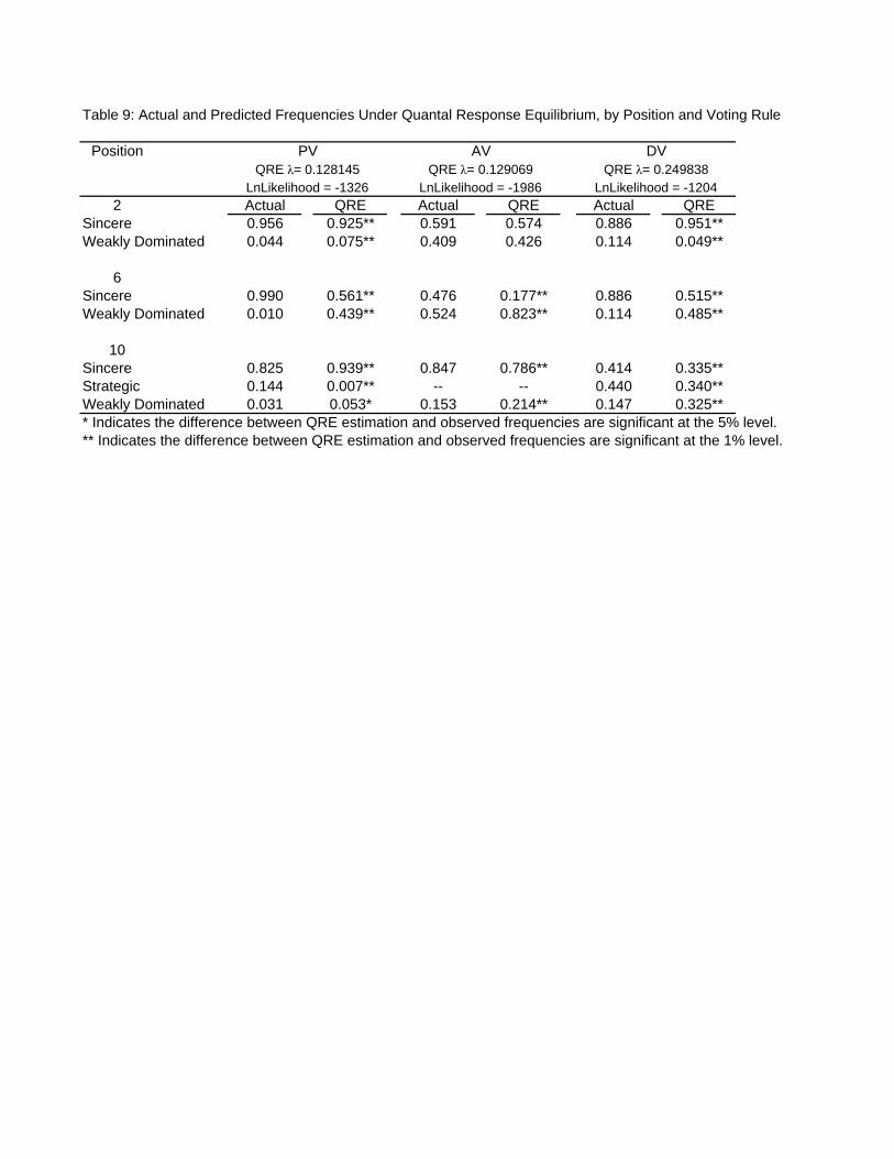
Table 9: Actual and Predicted Frequencies Under Quantal Response Equilibrium, by Position and Voting Rule

Position PV AV DVQRE λ= 0.128145 QRE λ= 0.129069 QRE λ= 0.249838

LnLikelihood = -1326 LnLikelihood = -1986 LnLikelihood = -12042 Actual QRE Actual QRE Actual QRE

Sincere 0.956 0.925** 0.591 0.574 0.886 0.951**Weakly Dominated 0.044 0.075** 0.409 0.426 0.114 0.049**

6Sincere 0.990 0.561** 0.476 0.177** 0.886 0.515**Weakly Dominated 0.010 0.439** 0.524 0.823** 0.114 0.485**

10Sincere 0.825 0.939** 0.847 0.786** 0.414 0.335**Strategic 0.144 0.007** -- -- 0.440 0.340**Weakly Dominated 0.031 0.053* 0.153 0.214** 0.147 0.325*** Indicates the difference between QRE estimation and observed frequencies are significant at the 5% level.** Indicates the difference between QRE estimation and observed frequencies are significant at the 1% level.

Table 10: Preferred Strategies Under Level-k Reasoning

Position PV AV DVLevel 1 Level 2+ Level 1 Level 2+ Level 1 Level 2+

2 G or O O G and O G and O G and O G and O6 O or B B O and B O and B O and B O and B10 B B B B O and B G and B

The colored alternatives are located at: (G)reen -- 1, (O)range -- 3, (B)lue -- 9

Table 11: Nash and Weak Undominance Nash Equilibria, by Voting Rule and Session

all early late all early latePV 0.996 1.000 0.993 0.996 1.000 0.993

(0.004) (0.000) (0.007) (0.004) (0.000) (0.069)

PV1 1.000 1.000 1.000 1.000 1.000 1.000(0.000) (0.000) (0.000) (0.000) (0.000) (0.000)

PV2 1.000 1.000 1.000 1.000 1.000 1.000(0.000) (0.000) (0.000) (0.000) (0.000) (0.000)

PV3 0.982 1.000 0.969 0.982 1.000 0.969(0.018) (0.000) (0.033) (0.018) (0.000) (0.033)

PV4 1.000 1.000 1.000 1.000 1.000 1.000(0.000) (0.000) (0.000) (0.000) (0.000) (0.000)

AV 0.957 0.948 0.963 0.681 0.583 0.750(0.013) (0.023) (0.016) (0.031) (0.050) (0.037)

AV1 1.000 1.000 1.000 0.781 0.583 0.900(0.000) (0.000) (0.000) (0.052) (0.101) (0.048)

AV2 0.946 0.875 1.000 0.714 0.708 0.719(0.030) (0.068) (0.000) (0.060) (0.093) (0.085)

AV3 0.929 0.917 0.938 0.679 0.542 0.781(0.034) (0.056) (0.046) (0.063) (0.102) (0.078)

AV4 0.946 1.000 0.906 0.536 0.500 0.563(0.030) (0.000) (0.055) (0.067) (0.102) (0.094)

DV 0.905 0.823 0.963 0.776 0.677 0.846(0.019) (0.045) (0.016) (0.027) (0.048) (0.031)

DV1 0.891 0.708 1.000 0.734 0.542 0.850(0.039) (0.093) (0.000) (0.055) (0.102) (0.057)

DV2 0.875 0.792 0.938 0.732 0.625 0.813(0.044) (0.083) (0.043) (0.059) (0.099) (0.074)

DV3 1.000 1.000 1.000 0.929 0.958 0.906(0.000) (0.000) (0.000) (0.034) (0.041) (0.055)

DV4 0.857 0.792 0.906 0.714 0.583 0.813(0.047) (0.083) (0.052) (0.060) (0.101) (0.074)

Numbers in parenthesis are the standard errors

% NE Outcomes % WUNE Outcomes

Table 12: Share of Three Way Ties in Election Outcomes, by Session

Three-way ties, shareall early late

PV 0.004 0.000 0.007(0.004) (0.000) (0.007)

PV1 0.000 0.000 0.000(0.000) (0.000) (0.000)

PV2 0.000 0.000 0.000(0.000) (0.000) (0.000)

PV3 0.018 0.000 0.031(0.018) (0.000) (0.033)

PV4 0.000 0.000 0.000(0.000) (0.000) (0.000)

AV 0.030 0.031 0.029(0.011) (0.018) (0.014)

AV1 0.000 0.000 0.000(0.000) (0.000) (0.000)

AV2 0.036 0.083 0.000(0.025) (0.057) (0.000)

AV3 0.054 0.042 0.063(0.030) (0.041) (0.046)

AV4 0.036 0.000 0.063(0.025) (0.000) (0.046)

DV 0.138 0.052 0.199(0.023) (0.023) (0.034)

DV1 0.203 0.083 0.275(0.050) (0.057) (0.071)

DV2 0.143 0.083 0.188(0.047) (0.057) (0.074)

DV3 0.125 0.000 0.219(0.044) (0.000) (0.078)

DV4 0.071 0.042 0.094(0.034) (0.041) (0.055)

Numbers in parenthesis are the standard errors

Table 13: Frequencies of Each Alternative Appearing in the Winning Set, by Session

mean Green Orange Blue(stdv) all early late all early late all early late

PV 0.004 0.000 0.007 0.854 0.854 0.854 0.392 0.438 0.361(0.004) (0.000) (0.007) (0.023) (0.036) (0.029) (0.032) (0.051) (0.040)

PV1 0.000 0.000 0.000 0.969 1.000 0.950 0.266 0.250 0.275(0.000) (0.000) (0.000) (0.022) (0.000) (0.035) (0.055) (0.089) (0.071)

PV2 0.000 0.000 0.000 0.719 0.625 0.775 0.469 0.583 0.400(0.000) (0.000) (0.000) (0.056) (0.099) (0.066) (0.062) (0.101) (0.078)

PV3 0.018 0.000 0.031 0.839 0.875 0.813 0.482 0.417 0.531(0.018) (0.000) (0.031) (0.049) (0.068) (0.069) (0.067) (0.101) (0.088)

PV4 0.000 0.000 0.000 0.893 0.917 0.875 0.357 0.500 0.250(0.000) (0.000) (0.000) (0.041) (0.057) (0.059) (0.064) (0.102) (0.077)

AV 0.043 0.052 0.037 0.720 0.625 0.787 0.509 0.594 0.449(0.013) (0.023) (0.016) (0.029) (0.050) (0.035) (0.033) (0.051) (0.042)

AV1 0.000 0.000 0.000 0.781 0.583 0.900 0.359 0.458 0.300(0.000) (0.000) (0.000) (0.052) (0.101) (0.048) (0.060) (0.102) (0.073)

AV2 0.054 0.125 0.000 0.768 0.833 0.719 0.554 0.500 0.594(0.030) (0.068) (0.000) (0.057) (0.076) (0.080) (0.067) (0.102) (0.087)

AV3 0.071 0.083 0.063 0.732 0.583 0.844 0.500 0.625 0.406(0.034) (0.057) (0.043) (0.059) (0.101) (0.064) (0.067) (0.099) (0.087)

AV4 (0.054) (0.000) (0.094) (0.589) (0.500) (0.656) (0.643) (0.792) (0.531)(0.030) (0.000) (0.052) (0.066) (0.102) (0.084) (0.064) (0.083) (0.088)

DV 0.207 0.146 0.250 0.862 0.833 0.882 0.302 0.302 0.301(0.027) (0.036) (0.037) (0.023) (0.038) (0.027) (0.030) (0.047) (0.039)

DV1 0.234 0.125 0.300 0.828 0.792 0.850 0.453 0.542 0.400(0.053) (0.068) (0.073) (0.047) (0.083) (0.057) (0.062) (0.102) (0.078)

DV2 0.250 0.250 0.250 0.857 0.833 0.875 0.304 0.292 0.313(0.058) (0.089) (0.077) (0.047) (0.076) (0.059) (0.062) (0.093) (0.082)

DV3 0.161 0.000 0.281 0.929 0.958 0.906 0.161 0.042 0.250(0.049) (0.000) (0.080) (0.034) (0.041) (0.052) (0.049) (0.041) (0.077)

DV4 0.179 0.208 0.156 0.839 0.750 0.906 0.268 0.333 0.219(0.051) (0.083) (0.064) (0.049) (0.089) (0.052) (0.059) (0.097) (0.073)

Numbers in parenthesis are the standard errorsThe colored alternatives are located at: Green -- 1, Orange -- 3, Blue -- 9

Table 14: Ballots Cast by Participants in Position 10,by Session, percent

PV1 AV1 DV1Ballot All Early Late All Early Late All Early Late

Green only 2.34* 2.08* 2.50* 5.47* 2.08* 7.50* -- -- --Orange only 14.06** 18.75** 11.25** 10.94* 6.25* 13.75* -- -- --Blue only 81.25 75.00 85.00 64.84 62.50 66.25 -- -- --Green and Orange -- -- -- 2.34* 4.17* 1.25* 3.13* 6.25* 1.25*Green and Blue -- -- -- 2.34* 0.00* 3.75* 60.16** 50.00** 66.25**Orange and Blue -- -- -- 14.06 25.00 7.50 31.25 29.17 32.50All Three -- -- -- 0.00* 0.00* 0.00* -- -- --Abstain 2.34* 4.17* 1.25* 0.00* 0.00* 0.00* 5.47* 14.58* 0.00*Total 100.0 100.0 100.0 100.0 100.0 100.0 100.0 100.0 100.0

PV2 AV2 DV2Ballot All Early Late All Early Late All Early Late

Green only 0.00* 0.00* 0.00* 0.89* 0.00* 1.56* -- -- --Orange only 22.66** 16.67** 26.25** 0.89* 2.08* 0.00* -- -- --Blue only 76.56 81.25 73.75 86.61 83.33 89.06 -- -- --Green and Orange -- -- -- 0.00* 0.00* 0.00* 14.29* 8.33* 18.75*Green and Blue -- -- -- 8.93* 12.50* 6.25* 41.96** 41.67** 42.19**Orange and Blue -- -- -- 2.68 2.08 3.13 33.93 39.58 29.69All three -- -- -- 0.00* 0.00* 0.00* -- -- --Abstain 0.78* 2.08* 0.00* 0.00* 0.00* 0.00* 9.82* 10.42* 9.38*Total 100.0 100.0 100.0 100.0 100.0 100.0 100.0 100.0 100.0

PV3 AV3 DV3Ballot All Early Late All Early Late All Early Late

Green only 1.79* 4.17* 0.00* 0.89* 0.00* 1.56* -- -- --Orange only 8.93** 18.75** 1.56** 4.46* 2.08* 6.25* -- -- --Blue only 89.29 77.08 98.44 75.00 79.17 71.88 -- -- --Green and Orange -- -- -- 0.00* 0.00* 0.00* 5.36* 8.33* 3.13*Green and Blue -- -- -- 0.00* 0.00* 0.00* 38.39** 27.08** 46.88**Orange and Blue -- -- -- 17.86 18.75 17.19 45.54 58.33 35.94All Three -- -- -- 0.89* 0.00* 1.56* -- -- --Abstain 0.00* 0.00* 0.00* 0.89* 0.00* 1.56* 10.71* 6.25* 14.06*Total 100.0 100.0 100.0 100.0 100.0 100.0 100.0 100.0 100.0

PV4 AV4 DV4Ballot All Early Late All Early Late All Early Late

Green only 2.68* 2.08* 3.13* 4.46* 2.08* 6.25* -- -- --Orange only 10.71** 10.42** 10.94** 0.00* 0.00* 0.00* -- -- --Blue only 83.93 85.42 82.81 70.54 83.33 60.94 -- -- --Green and Orange -- -- -- 1.79* 0.00* 3.13* 3.57* 2.08* 4.69*Green and Blue -- -- -- 6.25* 4.17* 7.81* 33.04** 37.50** 29.69**Orange and Blue -- -- -- 8.04 8.33 7.81 56.25 52.08 59.38All Three -- -- -- 8.93* 2.08* 14.06* -- -- --Abstain 2.68* 2.08* 3.13* 0.00* 0.00* 0.00* 7.14* 8.33* 6.25*Total 100.0 100.0 100.0 100.0 100.0 100.0 100.0 100.0 100.0The colored alternatives are located at: Green -- 1, Orange -- 3, Blue -- 9* Indicates the ballot is weakly dominated.** Indicates the ballot is strategic.

Figure 1: Experimental Design: Number Line Representation

green orange blue

1 2 3 4 5 6 7 8 9 10X X XX X X

Figure 2: Distribution of Strategic Votes among Voters in Position 10 Under Dual Voting

0

2

4

6

8

10

12

14

0.0 0.1-20.0 20.1-40.0 40.1-60.0 60.1-80.0 80.1-100.0Percent Strategic Votes

Num

ber o

f Par

ticip

ants

Early

Late

Figure 3: Distribution of Weakly Dominated Votes among Voters, by Voting Rule

Plurality Voting

05

10152025303540

0.0 0.1-20.0 20.1-40.0 40.1-60.0 60.1-80.0 80.1-100.0Percent Weakly Dominated Votes

Num

ber o

f Par

ticip

ants

EarlyLate

Approval Voting

05

10152025303540

0.0 0.1-20.0 20.1-40.0 40.1-60.0 60.1-80.0 80.1-100.0Percent Weakly Dominated Votes

Num

ber o

f Pa

rtic

ipan

ts

EarlyLate

Dual Voting

0

5

10

15

20

25

30

35

40

0.0 0.1-20.0 20.1-40.0 40.1-60.0 60.1-80.0 80.1-100.0

Percent Weakly Dominated Votes

Num

ber o

f Par

ticip

ants

EarlyLate

Figure 5: Plurality Voting: QRE Predicted Strategies' Frequencies vs. Observed Frequencies

PV- Position 2

0

0.2

0.4

0.6

0.8

1

1.2

0.0001 0.001 0.01 0.1 1 10

Lambda

Prob

abili

ty

Green

G: Actual

Orange

O: Actual

Blue

B: Actual

Abstain

Abs: Actual

PV- Position 6

0

0.1

0.2

0.3

0.4

0.5

0.6

0.7

0.8

0.0001 0.001 0.01 0.1 1 10

Lambda

Prob

abili

ty

Green

G: Actual

Orange

O: Actual

Blue

B: Actual

Abstain

Abs: Actual

PV- Position 10

0

0.2

0.4

0.6

0.8

1

1.2

0.0001 0.001 0.01 0.1 1 10

Lambda

Prob

abili

ty

Green

G: Actual

Orange

O: Actual

Blue

B: Actual

Abstain

Abs: Actual

Figure 6: Approval Voting: QRE Predicted Strategies' Frequencies vs. Observed Frequencies

AV - Position 2

00.10.20.30.40.50.60.70.80.9

0.0001 0.001 0.01 0.1 1 10

Lambda

Prob

abili

ty

Green

G: Actual

Orange

O: Actual

Blue

B: Actual

Green & Orange

G&O: Actual

Green & Blue

G&B: Actual

Orange & Blue

O&B: Actual

All Three

All3: Actual

Abstain

AV - Position 6

00.050.1

0.150.2

0.250.3

0.350.4

0.450.5

0.0001 0.001 0.01 0.1 1 10

Lambda

Prob

abili

ty

Green

G: Actual

Orange

O: Actual

Blue

B: Actual

Green & Orange

G&O: Actual

Green & Blue

G&B: Actual

Orange & Blue

O&B: Actual

All Three

All3: Actual

Abstain

Abs: Actual

AV - Position 10

0

0.2

0.4

0.6

0.8

1

1.2

0.0001 0.001 0.01 0.1 1 10

Lambda

Prob

abili

ty

Green

G: Actual

Orange

O: Actual

Blue

B: Actual

Green & Orange

G&O: Actual

Green & Blue

G&B: Actual

Orange & Blue

O&B: Actual

All Three

All3: Actual

Abstain

Abs: Actual

Figure 7: Dual Voting: QRE Predicted Strategies' Frequencies vs. Observed Frequencies

DV - Position 2

0

0.2

0.4

0.6

0.8

1

1.2

0.0001 0.001 0.01 0.1 1 10

Lambda

Prob

abili

ty

Green & Orange

G&O: Actual

Green & Blue

G&B: Actual

Orange & Blue

O&B: Actual

Abstain

Abs: Actual

DV - Position 6

0

0.2

0.4

0.6

0.8

1

1.2

0.0001 0.001 0.01 0.1 1 10

Lambda

Prob

abili

ty

Green & Orange

G&O: Actual

Green & Blue

G&B: Actual

Orange & Blue

O&B: Actual

Abstain

Abs: Actual

DV - Position 10

0

0.2

0.4

0.6

0.8

1

1.2

0.0001 0.001 0.01 0.1 1 10

Lambda

Prob

abili

ty

Green & Orange

G&O: Actual

Green & Blue

G&B: Actual

Orange & Blue

O&B: Actual

Abstain

Abs: Actual