multiple tests, multivariable decision rules, and prognostic tests michael a. kohn, md, mpp...
TRANSCRIPT

Multiple Tests, Multivariable Decision Rules, and Prognostic
Tests
Michael A. Kohn, MD, MPP
10/25/2007
Chapter 8 – Multiple Tests and Multivariable Decision Rules
Chapter 7 – Prognostic and Genetic Tests

Digression: Screening
Merenstein, “Winners and Losers,” about his experience being sued in 2002 by a man with incurable prostate cancer for not obtaining a prostate-specific antigen (PSA) test in 1999 when the man was 53 years old.
Hard copy handed out last week and posted on course website.
Discuss in section today?

Outline of Topics• Combining Tests
– Importance of test non-independence– Recursive Partitioning– Logistic Regression– Variable (Test) Selection– Importance of validation separate from derivation
• Prognostic tests– Differences from diagnostic tests and risk factors– Quantifying prediction: calibration and discrimination – Value of prognostic information– Common problems with studies of prognostic tests

Combining TestsExample
Prenatal sonographic Nuchal Translucency (NT) and Nasal Bone Exam (NBE) as dichotomous tests for Trisomy 21*
*Cicero, S., G. Rembouskos, et al. (2004). "Likelihood ratio for trisomy 21 in fetuses with absent nasal bone at the 11-14-week scan." Ultrasound Obstet Gynecol 23(3): 218-23.

If NT ≥ 3.5 mm Positive for Trisomy 21*
*What’s wrong with this definition?

>95th Perc.37.9%, 88.6%
> 3.5 mm9.2%, 63.7%
> 4.5 mm3.5%, 43.5%
> 5.5 mm1.9%, 31.2%
0%
10%
20%
30%
40%
50%
60%
70%
80%
90%
100%
0% 10% 20% 30% 40% 50% 60% 70% 80% 90% 100%
1 - Specificity
Sen
siti
vity
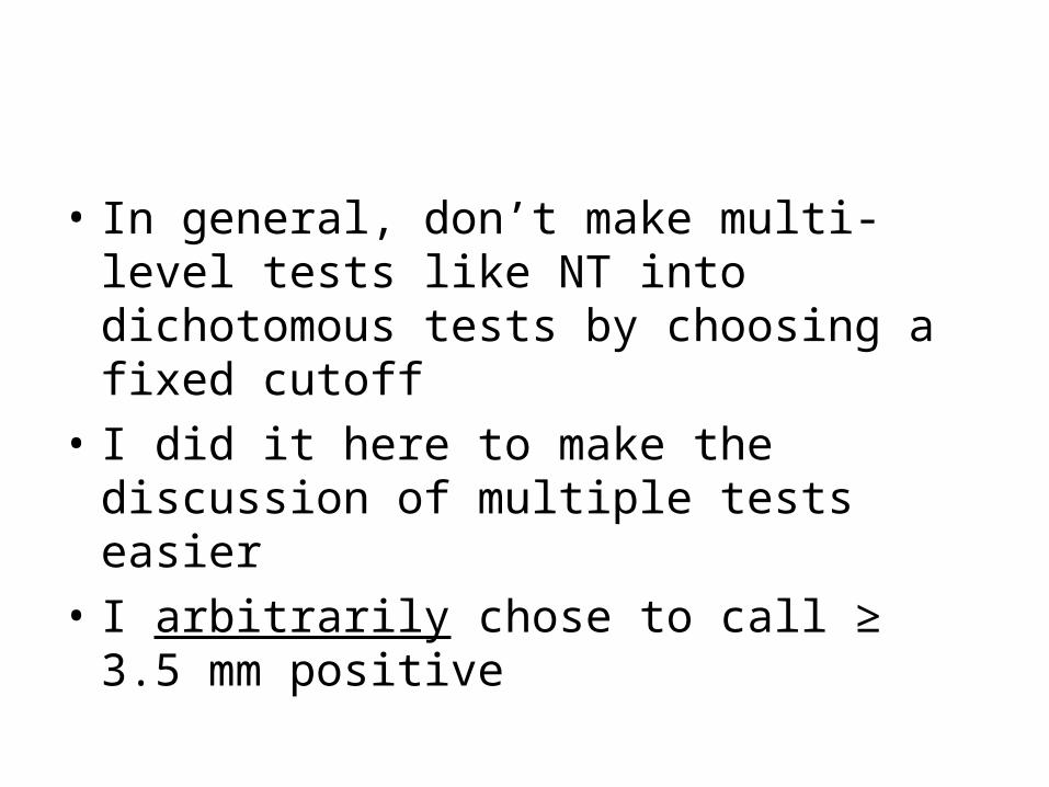
• In general, don’t make multi-level tests like NT into dichotomous tests by choosing a fixed cutoff
• I did it here to make the discussion of multiple tests easier
• I arbitrarily chose to call ≥ 3.5 mm positive

One Dichotomous Test
Trisomy 21
Nuchal D+ D- LR
Translucency
≥ 3.5 mm 212 478 7.0
< 3.5 mm 121 4745 0.4
Total 333 5223
Do you see that this is (212/333)/(478/5223)?
Review of Chapter 3: What are the sensitivity, specificity, PPV, and NPV of this test? (Be careful.)

Nuchal Translucency
• Sensitivity = 212/333 = 64%
• Specificity = 4745/5223 = 91%
• Prevalence = 333/(333+5223) = 6%
(Study population: pregnant women about to under go CVS, so high prevalence of Trisomy 21)
PPV = 212/(212 + 478) = 31%
NPV = 4745/(121 + 4745) = 97.5%** Not that great; prior to test P(D-) = 94%

Clinical Scenario – One TestPre-Test Probability of Down’s = 6%
NT Positive
Pre-test prob: 0.06
Pre-test odds: 0.06/0.94 = 0.064
LR(+) = 7.0
Post-Test Odds = Pre-Test Odds x LR(+)
= 0.064 x 7.0 = 0.44
Post-Test prob = 0.44/(0.44 + 1) = 0.31
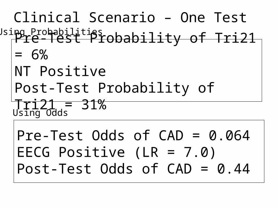
Pre-Test Probability of Tri21 = 6%NT PositivePost-Test Probability of Tri21 = 31%
Clinical Scenario – One Test
Pre-Test Odds of CAD = 0.064EECG Positive (LR = 7.0)Post-Test Odds of CAD = 0.44
Using Probabilities
Using Odds

Clinical Scenario – One TestPre-Test Probability of Tri21 = 6%
NT Positive
NT + (LR = 7.0) |--------------->
+-------------------------X---------------X------------------------------+ | | | | | | | Log(Odds) 2 -1.5 -1 -0.5 0 0.5 1 Odds 1:100 1:33 1:10 1:3 1:1 3:1 10:1 Prob 0.01 0.03 0.09 0.25 0.5 0.75 0.91
Odds = 0.064Prob = 0.06
Odds = 0.44Prob = 0.31

Nasal Bone SeenNBE Negativefor Trisomy 21
Nasal Bone AbsentNBE Positive
for Trisomy 21

Second Dichotomous Test
Nasal Bone Tri21+ Tri21- LR
Absent 229 129 27.8
Present 104 5094 0.32
Total 333 5223
Do you see that this is (229/333)/(129/5223)?

Pre-Test Probability of Trisomy 21 = 6%NT Positive for Trisomy 21 (≥ 3.5 mm)Post-NT Probability of Trisomy 21 = 31%NBE Positive for Trisomy 21 (no bone seen)Post-NBE Probability of Trisomy 21 = ?
Clinical Scenario –Two Tests
Using Probabilities

Clinical Scenario – Two Tests
Pre-Test Odds of Tri21 = 0.064NT Positive (LR = 7.0)Post-Test Odds of Tri21 = 0.44NBE Positive (LR = 27.8?)Post-Test Odds of Tri21 = .44 x 27.8?
= 12.4? (P = 12.4/(1+12.4) = 92.5%?)
Using Odds

Clinical Scenario – Two TestsPre-Test Probability of Trisomy 21 = 6%NT ≥ 3.5 mm AND Nasal Bone Absent
Odds = 0.064Prob = 0.06
Odds = 0.44Prob = 0.31
NT + (LR = 7.0) |---------------> NBE + (LR = 27.8) |---------------------------> NT + NBE + Can we do this? |--------------->|---------------------------> NT + and NBE + +---------------X----------------X----------------------------X-+ | | | | | | | Log(Odds) 2 -1.5 -1 -0.5 0 0.5 1 Odds 1:100 1:33 1:10 1:3 1:1 3:1 10:1 Prob 0.01 0.03 0.09 0.25 0.5 0.75 0.91
Odds = 12.4Prob = 0.925

Question
Can we use the post-test odds after a positive Nuchal Translucency as the pre-test odds for the positive Nasal Bone Examination?
i.e., can we combine the positive results by multiplying their LRs?
LR(NT+, NBE +) = LR(NT +) x LR(NBE +) ? = 7.0 x 27.8 ? = 194 ?

Answer = No
NT NBE
Trisomy 21
+ %
Trisomy 21
- % LR
Pos Pos 158 47% 36 0.7% 69
Pos Neg 54 16% 442 8.5% 1.9
Neg Pos 71 21% 93 1.8% 12
Neg Neg 50 15% 4652 89% 0.2
Total Total 333 100% 5223 100%
Not 194
158/(158 + 36) = 81%, not 92.5%

Non-Independence
Absence of the nasal bone does not tell you as much if you already know that the nuchal translucency is ≥ 3.5 mm.

Clinical Scenario
Pre-Test Odds of Tri21 = 0.064NT+/NBE + (LR =68.8)Post-Test Odds = 0.064 x 68.8
= 4.40 (P = 4.40/(1+4.40) = 81%, not 92.5%)
Using Odds
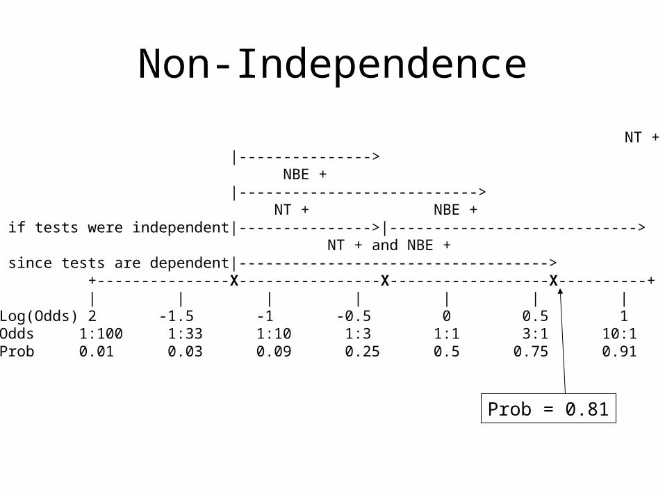
Non-Independence
NT + |---------------> NBE + |---------------------------> NT + NBE + if tests were independent|--------------->|----------------------------> NT + and NBE + since tests are dependent|-----------------------------------> +---------------X----------------X------------------X----------+ | | | | | | | Log(Odds) 2 -1.5 -1 -0.5 0 0.5 1 Odds 1:100 1:33 1:10 1:3 1:1 3:1 10:1 Prob 0.01 0.03 0.09 0.25 0.5 0.75 0.91
Prob = 0.81

Non-Independence of NT and NBE
Apparently, even in chromosomally normal fetuses, enlarged NT and absence of the nasal bone are associated. A false positive on the NT makes a false positive on the NBE more likely. Of normal (D-) fetuses with NT < 3.5 mm only 2.0% had nasal bone absent. Of normal (D-) fetuses with NT ≥ 3.5 mm, 7.5% had nasal bone absent.
Some (but not all) of this may have to do with ethnicity. In this London study, chromosomally normal fetuses of “Afro-Caribbean” ethnicity had both larger NTs and more frequent absence of the nasal bone.
In Trisomy 21 (D+) fetuses, normal NT was associated with the presence of the nasal bone, so a false negative on the NT was associated with a false negative on the NBE.

Non-Independence
Instead of looking for the nasal bone, what if the second test were just a repeat measurement of the nuchal translucency?
A second positive NT would do little to increase your certainty of Trisomy 21. If it was false positive the first time around, it is likely to be false positive the second time.
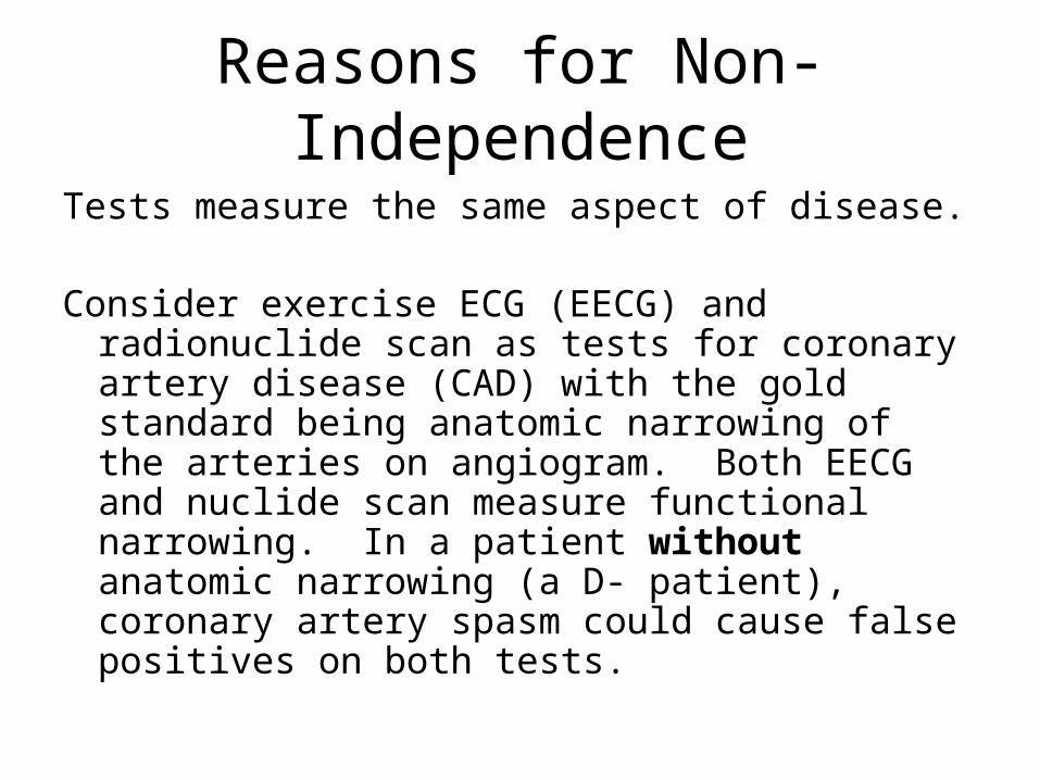
Reasons for Non-Independence
Tests measure the same aspect of disease.
Consider exercise ECG (EECG) and radionuclide scan as tests for coronary artery disease (CAD) with the gold standard being anatomic narrowing of the arteries on angiogram. Both EECG and nuclide scan measure functional narrowing. In a patient without anatomic narrowing (a D- patient), coronary artery spasm could cause false positives on both tests.
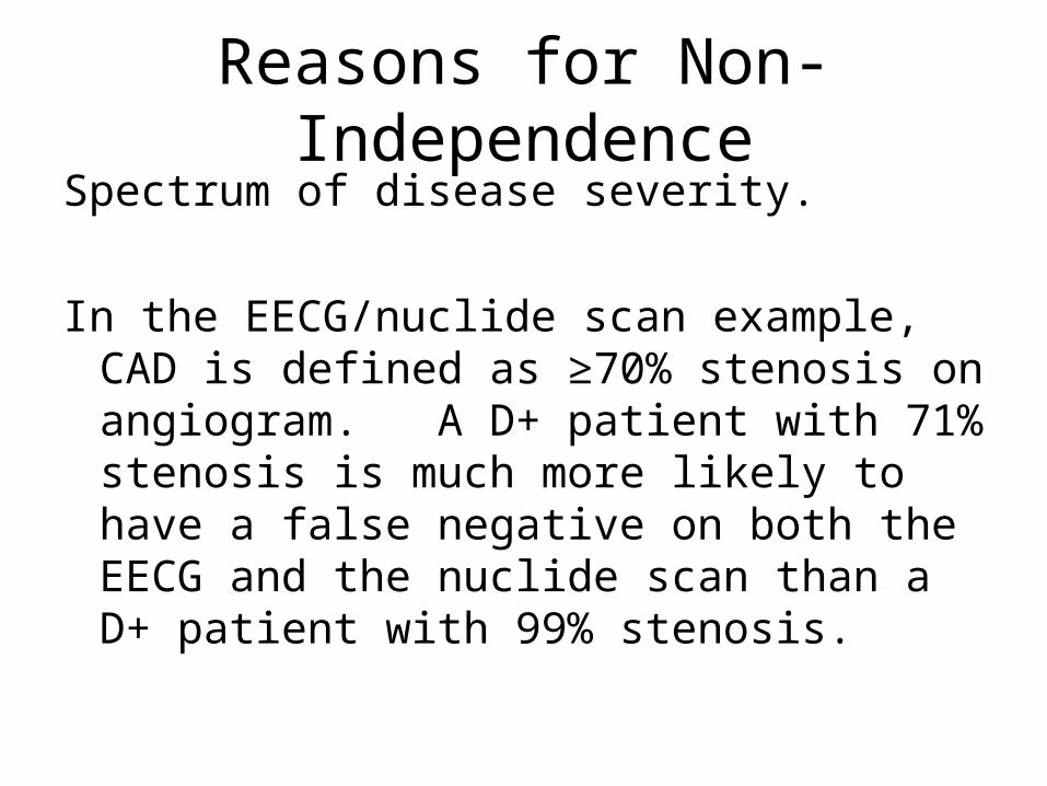
Reasons for Non-IndependenceSpectrum of disease severity.
In the EECG/nuclide scan example, CAD is defined as ≥70% stenosis on angiogram. A D+ patient with 71% stenosis is much more likely to have a false negative on both the EECG and the nuclide scan than a D+ patient with 99% stenosis.

Reasons for Non-IndependenceSpectrum of non-disease severity.
In this example, CAD is defined as ≥70% stenosis on angiogram. A D- patient with 69% stenosis is much more likely to have a false positive on both the EECG and the nuclide scan than a D- patient with 33% stenosis.

Counterexamples: Possibly Independent Tests
For Venous Thromboembolism:
• CT Angiogram of Lungs and Doppler Ultrasound of Leg Veins
• Alveolar Dead Space and D-Dimer
• MRA of Lungs and MRV of leg veins

Unless tests are independent, we can’t combine results by
multiplying LRs

Ways to Combine Multiple TestsOn a group of patients (derivation set),
perform the multiple tests and (independently*) determine true disease status (apply the gold standard)
• Measure LR for each possible combination of results
• Recursive Partitioning
• Logistic Regression
*Beware of incorporation bias

Determine LR for Each Result Combination
NT NBE Tri21+ % Tri21- % LRPost Test
Prob*
Pos Pos 158 47% 36 0.7% 69 81%
Pos Neg 54 16% 442 8.5% 1.9 11%
Neg Pos 71 21% 93 1.8% 12 43%
Neg Neg 50 15% 4652 89.1% 0.2 1%
Total Total 333 100% 5223 100%
*Assumes pre-test prob = 6%

Determine LR for Each Result Combination
2 dichotomous tests: 4 combinations
3 dichotomous tests: 8 combinations
4 dichotomous tests: 16 combinations
Etc.
2 3-level tests: 9 combinations
3 3-level tests: 27 combinations
Etc.

Determine LR for Each Result Combination
How do you handle continuous tests?
Not practical for most groups of tests.

Recursive PartitioningMeasure NT First
Nuchal Translucency
Nasal Bone
< 3.5 mm ≥ 3.5 mm
31%2.5%
Present
1 %
Suspected Trisomy 21 (P = 6%)
43 %
Nasal Bone
Absent Present
11 %
Absent
81 %
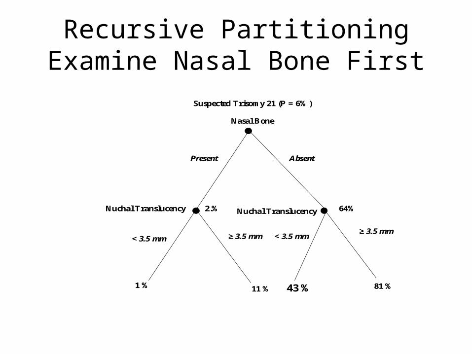
Recursive PartitioningExamine Nasal Bone First
Nasal Bone
Nuchal Translucency
< 3.5 mm≥ 3.5 mm
64%2.%
Present
1 %
Suspected Trisomy 21 (P = 6%)
11 % 43 %
Absent
81 %
< 3.5 mm≥ 3.5 mm
Nuchal Translucency

Recursive PartitioningExamine Nasal Bone FirstCVS if P(Trisomy 21 > 5%)
Nasal Bone
Nuchal Translucency
< 3.5 mm≥ 3.5 mm
64%2%
Present
1 %
Suspected Trisomy 21 (P = 6%)
11 % 43 %
Absent
81 %
< 3.5 mm≥ 3.5 mm
Nuchal Translucency
No NT, CVS
CVSNo CVS

Recursive PartitioningExamine Nasal Bone FirstCVS if P(Trisomy 21 > 5%)
Nasal Bone
Nuchal Translucency
< 3.5 mm
64%2%
Present
1 %
Suspected Trisomy 21 (P = 6% )
11 %
Absent
≥ 3.5 mmCVS
CVSNo CVS

Recursive Partioning
• Same as Classification and Regression Trees (CART)
• Don’t have to work out probabilities (or LRs) for all possible combinations of tests, because of “tree pruning”

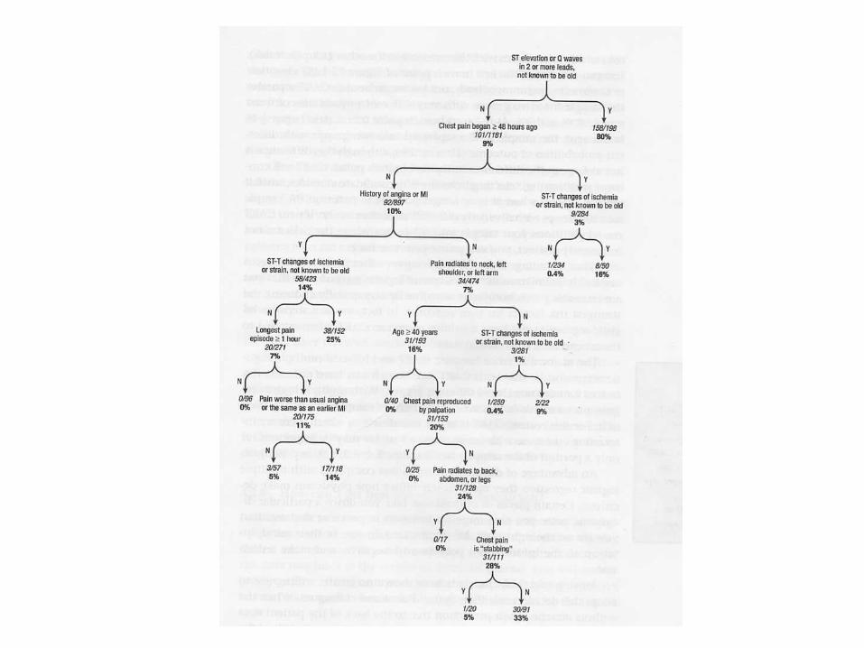
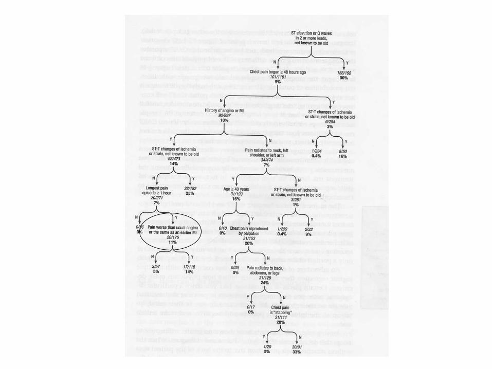
Tree Pruning: Goldman Rule*
8 “Tests” for Acute MI in ER Chest Pain Patient :1. ST Elevation on ECG; 2. CP < 48 hours; 3. ST-T changes on ECG; 4. Hx of MI; 5. Radiation of Pain to Neck/LUE; 6. Longest pain > 1 hour; 7. Age > 40 years; 8. CP not reproduced by palpation.
*Goldman L, Cook EF, Brand DA, et al. A computer protocol to predict myocardial infarction in emergency department patients with chest pain. N Engl J Med. 1988;318(13):797-803.

ST Elevation
CP < 48 hrs No Yes
14%No
9 %
10 %
YesNo
Yes
80 %CP < 48 hrs
No Yes No YesHx of ACI Hx of ACI Hx of ACI Hx of ACI
YesST Changes
No7% 25 %
CP > 1 hr CP > 1 hr
No NoYes Yes0% 11%
No YesNo Yes
8 tests 28 = 256 Combinations

Recursive Partitioning
• Does not deal well with continuous test results*
*when there is a monotonic relationship between the test result and the probability of disease

Logistic Regression
Ln(Odds(D+)) =
a + bNTNT+ bNBENBE + binteract(NT)(NBE)
“+” = 1
“-” = 0
More on this later in ATCR!

Why does logistic regression model log-odds instead of probability?
Related to why the LR Slide Rule’s log-odds scale helps us visualize combining test results.

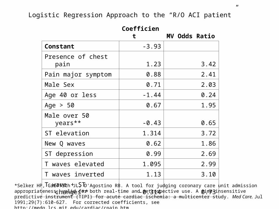
Logistic Regression Approach to the “R/O ACI patient”
*Selker HP, Griffith JL, D'Agostino RB. A tool for judging coronary care unit admission appropriateness, valid for both real-time and retrospective use. A time-insensitive predictive instrument (TIPI) for acute cardiac ischemia: a multicenter study. Med Care. Jul 1991;29(7):610-627. For corrected coefficients, see http://medg.lcs.mit.edu/cardiac/cpain.htm
Coefficient MV Odds Ratio
Constant -3.93
Presence of chest pain 1.23 3.42
Pain major symptom 0.88 2.41
Male Sex 0.71 2.03
Age 40 or less -1.44 0.24
Age > 50 0.67 1.95
Male over 50 years** -0.43 0.65
ST elevation 1.314 3.72
New Q waves 0.62 1.86
ST depression 0.99 2.69
T waves elevated 1.095 2.99
T waves inverted 1.13 3.10
T wave + ST changes** -0.314 0.73

Clinical Scenario*
71 y/o man with 2.5 hours of CP, substernal, non-radiating, described as “bloating.” Cannot say if same as prior MI or worse than prior angina.
Hx of CAD, s/p CABG 10 yrs prior, stenting 3 years and 1 year ago. DM on Avandia.
ECG: RBBB, Qs inferiorly. No ischemic ST-T changes.
*Real patient seen by MAK 1 am 10/12/04

Coefficient Clinical Scenario
Constant -3.93 Result -3.93
Presence of chest pain 1.23 1 1.23
Pain major symptom 0.88 1 0.88
Sex 0.71 1 0.71
Age 40 or less -1.44 0 0
Age > 50 0.67 1 0.67
Male over 50 years -0.43 1 -0.43
ST elevation 1.314 0 0
New Q waves 0.62 0 0
ST depression 0.99 0 0
T waves elevated 1.095 0 0
T waves inverted 1.13 0 0
T wave + ST changes -0.314 0 0
-0.87
Odds of ACI 0.418952
Probability of ACI 30%
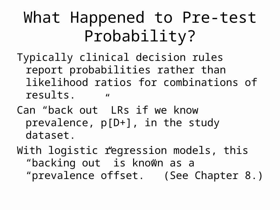
What Happened to Pre-test Probability?
Typically clinical decision rules report probabilities rather than likelihood ratios for combinations of results.
Can “back out” LRs if we know prevalence, p[D+], in the study dataset.
With logistic regression models, this “backing out” is known as a “prevalence offset.” (See Chapter 8.)
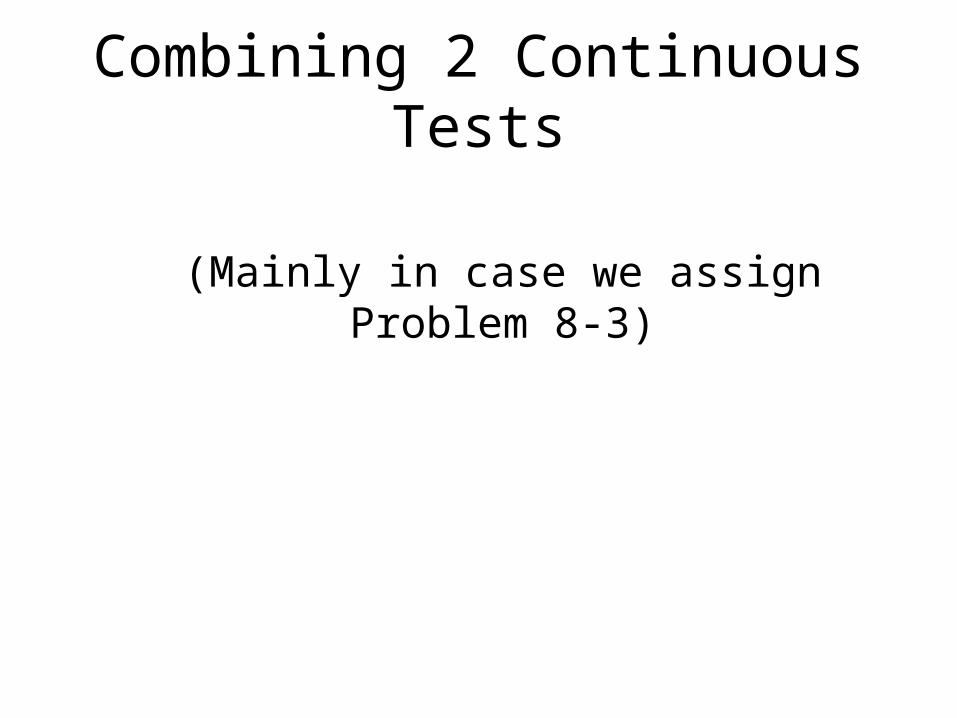
Combining 2 Continuous Tests
(Mainly in case we assign Problem 8-3)

Optimal Cutoff Line for Two Continuous Tests

Optimal Cutoff for a Single Continuous Test
Depends on
1) Pre-test Probability of Disease
2) ROC Curve (Likelihood Ratios)
3) Relative Misclassification Costs
Cannot choose an optimal cutoff with just the ROC curve.

Effect of Prevalence
0500
100015002000250030003500
35 36 37 38 39 40
Gestational Age (weeks)
Bir
th W
eig
ht
(gra
ms)
Prevalence = 4.6% Prevalence = 2%
Low Risk
High Risk

Choosing Which Tests to Include in the Decision Rule
Have focused on how to combine results of two or more tests, not on which of several tests to include in a decision rule.
Variable Selection Options include:
• Recursive partitioning
• Automated stepwise logistic regression
Choice of variables in derivation data set requires confirmation in a separate validation data set.
Variable Selection
• Especially susceptible to overfitting

Need for Validation: Example*Study of clinical predictors of bacterial diarrhea.Evaluated 34 historical items and 16 physical
examination questions. 3 questions (abrupt onset, > 4 stools/day, and
absence of vomiting) best predicted a positive stool culture (sensitivity 86%; specificity 60% for all 3).
Would these 3 be the best predictors in a new dataset? Would they have the same sensitivity and specificity?
*DeWitt TG, Humphrey KF, McCarthy P. Clinical predictors of acute bacterial diarrhea in young children. Pediatrics. Oct 1985;76(4):551-556.

Need for ValidationDevelop prediction rule by choosing a few
tests and findings from a large number of possibilities.
Takes advantage of chance variations* in the data.
Predictive ability of rule will probably disappear when you try to validate on a new dataset.
Can be referred to as “overfitting.”
e.g., low serum calcium in 12 children with hemolytic uremic syndrome and bad outcomes

VALIDATION
No matter what technique (CART or logistic regression) is used, the tests included in a “rule” and the way in which their results are combined must be tested on a data set different from the one used to derive the rule.
Beware of studies that use a “validation set” to “tweak” the rule. This is really just a second derivation step.

Prognostic Tests
Chapter 7

Assessment of Prognostic Tests
• Difference from diagnostic tests and risk factors
• Quantifying accuracy (calibration and discrimination)
• Value of prognostic information
• Common problems with studies of prognostic tests

Potential confusion: “cross-sectional” means 2 things
• Cross-sectional sampling means sampling does not depend on either the predictor variable or the outcome variable. (E.g., as opposed to case-control sampling)
• Cross-sectional time dimension means that predictor and outcome are measured at the same time -- opposite of longitudinal

Cohort Studies Start with a Cross-Sectional Study
(Substitute “Outcome” for “Disease”)
Eliminate subjects who already have disease

Difference from Diagnostic Tests
• Longitudinal rather than cross-sectional time dimension
• Incidence rather than prevalence• Sensitivity, specificity, prior probability confusing• Time to an event may be important• Harder to quantify accuracy in individuals
– Exceptions: short time course, continuous outcomes

Difference from Risk Factors
• Causality not important
• Absolute risk very important– Sampling scheme makes a much bigger
difference because absolute risks are less generalizable than relative risks
– Can be informative even if no bad outcomes!

• How accurate are the predicted probabilities?– Break the population into groups– Compare actual and predicted probabilities
for each group
• Calibration is important for decision making and giving information to patients
Quantifying Prediction 1: Calibration

• How well can the test separate subjects in the population from the mean probability to values closer to zero or 1?
• May be more generalizable
• Often measured with C-statistic
Quantifying Prediction 2: Discrimination

Illustrations
• Perfect calibration, no discrimination:– Predicted = actual 5-year mortality = 45% (for
everyone)
• Perfect discrimination, poor calibration– Overall predicted mortality* is 15%, but every
patient who dies has a predicted mortality > 20% and every patient who survives has a predicted mortality of < 20%
* ∑Pi(mortality) / N
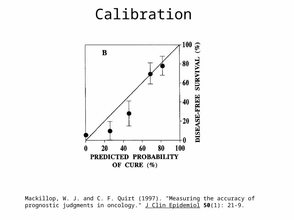
Calibration
Mackillop, W. J. and C. F. Quirt (1997). "Measuring the accuracy of prognostic judgments in oncology." J Clin Epidemiol 50(1): 21-9.

Calibration
Glare, P., K. Virik, et al. (2003). "A systematic review of physicians' survival predictions in terminally ill cancer patients." Bmj 327(7408): 195-8.

Quantifying Discrimination:
• Dichotomize outcome at time t
• Then can calculate– Sensitivity and specificity– Likelihood ratios– ROC curves, c-statistic– Can provide these for multiple time points. In
each case, probabilities are for an event on or before time t.

Discrimination
Mackillop, W. J. and C. F. Quirt (1997). "Measuring the accuracy of prognostic judgments in oncology." J Clin Epidemiol 50(1): 21-9.
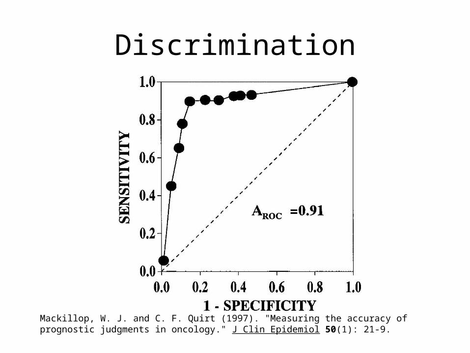
Discrimination
Mackillop, W. J. and C. F. Quirt (1997). "Measuring the accuracy of prognostic judgments in oncology." J Clin Epidemiol 50(1): 21-9.
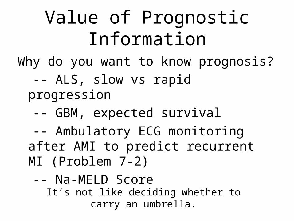
Value of Prognostic Information
Why do you want to know prognosis?
-- ALS, slow vs rapid progression
-- GBM, expected survival
-- Ambulatory ECG monitoring after AMI to predict recurrent MI (Problem 7-2)
-- Na-MELD Score
It’s not like deciding whether to carry an umbrella.

Value of Prognostic Information
• To inform treatment or other clinical decisions
• To inform (prepare) patients and their families
• To stratify by disease severity in clinical trials
Altman, D. G. and P. Royston (2000). "What do we mean by validating a prognostic model?" Stat Med 19(4): 453-73.

• Doctors and patients like prognostic information
• But hard to assess its value• Most objective approach is decision-
analytic. Consider: – What decision is to be made– Costs of errors– Cost of test
Value of Prognostic Information

• DECISION: Treat with more aggressive regimen
• BEFORE test: 5-year mortality = 25%• AFTER test: 5-year mortality either 10% or 50%• BUT: do we know how bad it is:
– To treat patient with 10% mortality with more aggressive regimen?
– To treat patient with 50% mortality with less aggressive regimen?
Example

Common Problems with Studies of Prognostic Tests- 1
• Referral/selection bias – e.g. too many studies from tertiary centers
• Poorly defined cohort; heterogeneous inclusion criteria – (See Problem 7-1 about predicting neurologic and audiologic sequelae in congenital CMV infection.)
• Effects of prognosis on treatment and effects of treatment on prognosis– Effective treatments blunt relationships– End-of-life decisions may accentuate relationships

Common Problems with Studies of Prognostic Tests- 2
• Multiple and composite outcomes– If multiple outcomes collected, is the one best
predicted highlighted?– If a study combines multiple outcomes, will the
composite outcome be dominated by the most frequent?
More on composite outcomes in Chapter 9 (next week)

Common Problems with Studies of Prognostic Tests- 3
• Loss to follow-up
• Blinding
Next week

Common Problems with Studies of Prognostic Tests- 4
• Overfitting – Already discussed– Which variables are included– How they are combined
• Inadequate sample size– Small sample size results in imprecise absolute risk estimates.
• Quantifying effect size– Watch for comparison of 1st and 5th quintiles, units for hazard or
odds ratios– How much NEW information?
• Frequently assessed with multivariable techniques
• Publication bias

Example: A multigene assay to predict recurrence of tamoxifen-treated, node-
negative breast cancer* • 10-year distant recurrence risk in low, medium,
high risk: 6.8%, 14.3%, and 30.5%• Hazard ratio 3.21 per 50 point change
– 51% had scores <12– Age, tumor size dichotomized– Tumor grade reproducibility only fair (κ=0.34-0.37)
• Authors of paper patented the test ($3500 charge)
*Paik et al. N Engl J Med 2004;351(27):2817-26.
Additional Slides
Prognostic Test Accuracy
Calibration and Discrimination
Should I carry an umbrella tomorrow?
Watch the weather man on TV tonight

Good Weather ManPredicted Chance of
RainDays
Expected Rainy Days
Actual Rainy Days
Actual Percent
Actual - Expected
0% 120 0 0 0% 0%
10% 91 9.1 1 1% -9%
20% 49 9.8 4 8% -12%
30% 20 6 7 35% 5%
40% 22 8.8 12 55% 15%
50% 21 10.5 14 67% 17%
60% 19 11.4 14 74% 14%
70% 14 9.8 12 86% 16%
80% 5 4 5 100% 20%
90% 3 2.7 3 100% 10%
100% 1 1 1 100% 0%
365 73.1 73

Calibration
0%
10%
20%
30%
40%
50%
60%
70%
80%
90%
100%
0% 10%
20%
30%
40%
50%
60%
70%
80%
90%
100%
Predicted Chance of Rain
Act
ual
Per
cen
t R
ain
y
Perfect Calibration
Good Weatherman
Calibration
-15%
-10%
-5%
0%
5%
10%
15%
20%
25%
0% 10%
20%
30%
40%
50%
60%
70%
80%
90%
100%
Predicted
Act
ual
- P
red
icte
d

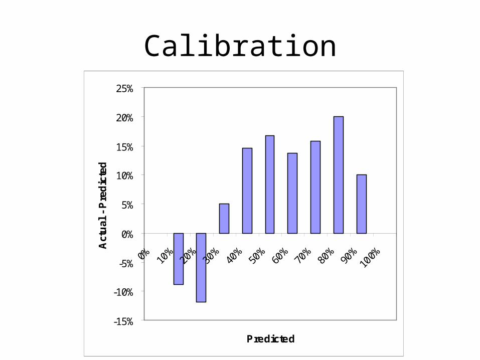
Bad Weather ManPredicted Chance of
RainDays
Expected Rainy Days
Actual Rainy Days
Actual Percent
Actual - Expected
0% 0 0 0
10% 100 10 10 10% 0%
20% 250 50 50 20% 0%
30% 0 0 0
40% 0 0 0
50% 0 0 0
60% 0 0 0
70% 0 0 0
80% 0 0 0
90% 15 13.5 13 87% -3%
100% 0 0 0
365 73.5 73

Calibration
0%
10%
20%
30%
40%
50%
60%
70%
80%
90%
100%
0% 10% 20% 30% 40% 50% 60% 70% 80% 90% 100%
Perfect Calibration
Actual

Calibration
-15%
-10%
-5%
0%
5%
10%
15%
20%
25%
0% 10%
20%
30%
40%
50%
60%
70%
80%
90%
100%
Predicted
Act
ual
- P
red
icte
d

Good Weather Man
0
0.1
0.2
0.3
0.4
0.5
0% 10%
20%
30%
40%
50%
60%
70%
80%
90%
100%
Predicted Chance of Rain
Fre
qu
en
cy Actual Rainy Days
Didn't Rain

Same Discrimination, Poor Calibration
0
0.1
0.2
0.3
0.4
0.5
50% 55% 60% 65% 70% 75% 80% 85% 90% 95% 100%
Predicted Chance of Rain
Fre
qu
ency
Actual Rainy DaysDidn't Rain
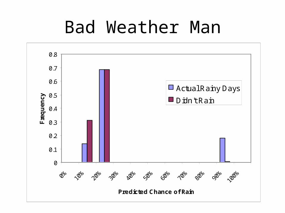
Bad Weather Man
0
0.1
0.2
0.3
0.4
0.5
0.6
0.7
0.8
0% 10%
20%
30%
40%
50%
60%
70%
80%
90%
100%
Predicted Chance of Rain
Fre
qu
ency
Actual Rainy Days
Didn't Rain

Compare Weathermen
0
0.1
0.2
0.3
0.4
0.5
0.6
0.7
0.8
0.9
1
0 0.1 0.2 0.3 0.4 0.5 0.6 0.7 0.8 0.9 1
False Positive Rate
Tru
e P
os
itiv
e R
ate
Good Weatherman
Bad Weatherman

Compare Weather Men
Failing to carry an umbrella on rainy day (“Wet”) just as bad as carrying an umbrella on a sunny day (“Tired”). Cutoff = 50% chance of rain
Good Weatherman: Wet = 24, Tired = 14, Total = 38
Bad Weatherman: Wet = 60, Tired = 2, Total = 62

Compare Weather Men
Failing to carry an umbrella on rainy day (“Wet”) 4X as bad as carrying an umbrella on a sunny day (“Tired”). Cutoff = 20% chance of rain.
Good Weatherman: Wet = 1, Tired = 82, Total = 1 × 4 + 82 = 86
Bad Weatherman: Wet = 10, Tired = 202, Total = 10 × 4 + 202 = 242