multiple modal biometricssnmrec.fau.edu/sites/default/files/research/theses/dt-10...biometrics is...
TRANSCRIPT

AUTOMATED BIOMETRICS OF AUDIO-VISUAL MULTIPLE MODALS
By
Lin Huang
A Dissertation Submitted to the Faculty of
The College of Engineering and Computer Science
in Fulfillment of the Requirements for the Degree of
Doctor of Philosophy
Florida Atlantic University
Boca Raton, FL
05/10/2010

ii
Copyright by Lin Huang 2010


iv
ACKNOWLEDGEMENTS
The author wishes to express her sincere thanks and love to her husband, son,
sisters, brother and parents for their support and encouragement throughout the writing of
this manuscript. The author is grateful to the committee members for providing their
superior supervision.

v
ABSTRACT
Author: Lin Huang
Title: Automated Biometrics of Audio-Visual Multiple Modals
Institution: Florida Atlantic University
Dissertation Advisor: Dr. Hanqi Zhuang
Degree: Doctor of Philosophy
Year: 2010
Biometrics is the science and technology of measuring and analyzing biological
data for authentication purposes. Its progress has brought in a large number of civilian
and government applications. The candidate modalities used in biometrics include
retinas, fingerprints, signatures, audio, faces, etc.
There are two types of biometric system: single modal systems and multiple modal
systems. Single modal systems perform person recognition based on a single biometric
modality and are affected by problems like noisy sensor data, intra-class variations,
distinctiveness and non-universality. Applying multiple modal systems that consolidate
evidence from multiple biometric modalities can alleviate those problems of single modal
ones.
Integration of evidence obtained from multiple cues, also known as fusion, is a
critical part in multiple modal systems, and it may be consolidated at several levels like
feature fusion level, matching score fusion level and decision fusion level.

vi
Among biometric modalities, both audio and face modalities are easy to use and
generally acceptable by users. Furthermore, the increasing availability and the low cost of
audio and visual instruments make it feasible to apply such Audio-Visual (AV) systems
for security applications. Therefore, this dissertation proposes an algorithm of face
recognition. In addition, it has developed some novel algorithms of fusion in different
levels for multiple modal biometrics, which have been tested by a virtual database and
proved to be more reliable and robust than systems that rely on a single modality.
vii
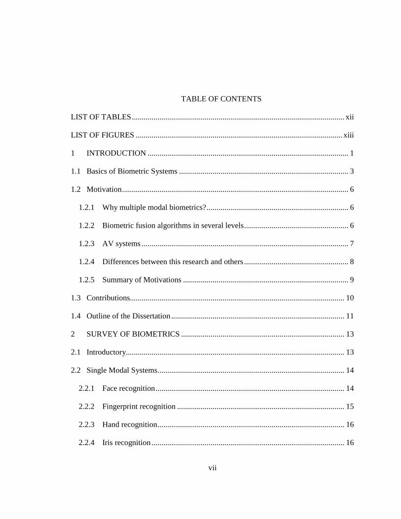
TABLE OF CONTENTS
LIST OF TABLES ............................................................................................................ xii
LIST OF FIGURES ......................................................................................................... xiii
1 INTRODUCTION ...................................................................................................... 1
1.1 Basics of Biometric Systems ...................................................................................... 3
1.2 Motivation ................................................................................................................... 6
1.2.1 Why multiple modal biometrics? ........................................................................ 6
1.2.2 Biometric fusion algorithms in several levels ..................................................... 6
1.2.3 AV systems ......................................................................................................... 7
1.2.4 Differences between this research and others ..................................................... 8
1.2.5 Summary of Motivations .................................................................................... 9
1.3 Contributions............................................................................................................. 10
1.4 Outline of the Dissertation ........................................................................................ 11
2 SURVEY OF BIOMETRICS ................................................................................... 13
2.1 Introductory............................................................................................................... 13
2.2 Single Modal Systems............................................................................................... 14
2.2.1 Face recognition ................................................................................................ 14
2.2.2 Fingerprint recognition ..................................................................................... 15
2.2.3 Hand recognition ............................................................................................... 16
2.2.4 Iris recognition .................................................................................................. 16

viii
2.2.5 Retina recognition ............................................................................................. 17
2.2.6 Signature recognition ........................................................................................ 17
2.2.7 Voice recognition .............................................................................................. 17
2.2.8 DNA .................................................................................................................. 18
2.2.9 Summary of single modal systems ................................................................... 18
2.3 Multiple Modal Systems ........................................................................................... 21
2.3.1 Multiple modal biometrics vs. single modal biometrics ................................... 21
2.3.2 Multiple modal biometric fusions ..................................................................... 24
2.3.3 Literature review ............................................................................................... 24
3 FACE RECOGNITION ............................................................................................ 31
3.1 Introduction ............................................................................................................... 31
3.2 Eigenface................................................................................................................... 35
3.3 Pyramidal Gabor Wavelets ....................................................................................... 37
3.4 PGE algorithm and analysis ...................................................................................... 40
3.4.1 PGE Algorithm ................................................................................................. 40
3.4.2 Algorithm Analysis ........................................................................................... 42
3.5 Experiment ................................................................................................................ 44
3.6 Summary ................................................................................................................... 48
4 VOICE RECOGNITION .......................................................................................... 49
4.1 Introduction ............................................................................................................... 49
4.2 Text-independent Speaker Recognition .................................................................... 51
4.2.1 Audio Feature Extraction .................................................................................. 52
4.2.2 Vector Quantization .......................................................................................... 54

ix
4.2.3 Gaussian Mixture Model................................................................................... 55
4.3 Experiment ................................................................................................................ 57
4.4 Summary ................................................................................................................... 58
5 BIOMETRICS FUSION ........................................................................................... 59
5.1 Introduction ............................................................................................................... 59
5.2 Information Fusion.................................................................................................... 60
5.3 Summary ................................................................................................................... 65
6 FUSION BY SYNCHRONIZATION OF FEATURE STREAMS .......................... 67
6.1 Introduction ............................................................................................................... 67
6.2 Feature Extraction of AVTI system .......................................................................... 69
6.2.1 Audio feature extraction ................................................................................... 69
6.2.2 Visual feature extraction ................................................................................... 70
6.3 Feature fusion............................................................................................................ 71
6.4 Experiments .............................................................................................................. 75
6.4.1 Experimental setup............................................................................................ 75
6.4.2 Results for the proposed method....................................................................... 76
6.5 Conclusion ................................................................................................................ 79
7 FUSION BY LINK MATRIX ALGORITHM AT FEATURE LEVEL .................. 80
7.1 Introduction ............................................................................................................... 80
7.2 Preliminaries ............................................................................................................. 82
7.3 A method to fuse features ......................................................................................... 83
7.4 Case Studies .............................................................................................................. 87
7.5 Proposed Classification Method ............................................................................... 90

x
7.5.1 AV identification based on least-squares algorithm ......................................... 90
7.5.2 AV identification based on analyzing pdfs ....................................................... 90
7.6 Experimental studies ................................................................................................. 92
7.6.1 Experiment setup .............................................................................................. 92
7.6.2 LS vs. RBF-liked classification ........................................................................ 92
7.6.3 Robustness of the proposed method ................................................................. 93
7.7 Conclusion ................................................................................................................ 95
8 FUSION BY GENETIC ALGORITHM AT FEATURE LEVEL ........................... 96
8.1 Introduction ............................................................................................................... 96
8.2 Proposed GA fusion method ..................................................................................... 98
8.3 AV Case Studies ..................................................................................................... 104
8.4 Conclusion .............................................................................................................. 108
9 FUSION BY SIMULATED ANNEALING AT FEATURE LEVEL .................... 109
9.1 Introduction ............................................................................................................. 109
9.2 Fusion based on simulated annealing ..................................................................... 110
9.2.1 Fusions ............................................................................................................ 110
9.2.2 Proposed model of biometric fusion ............................................................... 111
9.2.3 SA regulation algorithm .................................................................................. 112
9.3 A case study: audio-visual biometric system .......................................................... 119
9.3.1 AV feature extraction ...................................................................................... 119
9.3.2 Experiment ...................................................................................................... 120
9.4 Conclusions ............................................................................................................. 124
10 FUSION AT SCORE LEVEL ................................................................................ 125

xi
10.1 Introduction ............................................................................................................. 125
10.2 Proposed Methods ................................................................................................... 127
10.2.1 Golden Ratio Basics .................................................................................... 129
10.2.2 Proposed golden ratio method .................................................................... 130
10.3 Case Study: Audio-visual Biometric System .......................................................... 131
10.3.1 AV feature extraction .................................................................................. 131
10.3.2 Experiment .................................................................................................. 132
10.4 Conclusion .............................................................................................................. 134
11 CONCLUSION ....................................................................................................... 136
12 APPENDIX ............................................................................................................. 138
13 REFERENCE .......................................................................................................... 157

xii
LIST OF TABLES
Table 1.1 General advantages/disadvantages of biometrics ............................................ 4
Table 2.1 Comparison of Various Biometrics ............................................................... 19
Table 2.2 Comparison of single modal system (continued) .......................................... 20
Table 2.3 Comparison of single modal systems (continued) ......................................... 21
Table 2.4 Review of multiple modal systems ................................................................ 25
Table 3.1 Filter masks .................................................................................................... 39
Table 3.2 Comparison among PGE, Eigenface and classic 2-D Gabor based methods 48
Table 4.1 Effect of various numbers of Gaussian models ............................................. 58
Table 6.1 Comparison for various methods ................................................................... 78
Table 6.2 Comparisons of the proposed method and MD method ................................ 78
Table 6.3 Recognition rate vs. length of AV feature vector .......................................... 79
Table 7.1 Patterns for subject S1, S2 and S3 in modality M2 .......................................... 89
Table 7.2 LS vs. RBF-like classification ....................................................................... 93
Table 7.3 Comparison result under various conditions ................................................. 94
Table 8.1 Comparison result under various conditions ............................................... 107
Table 8.2 Weights for visual part in the virtual AV system ........................................ 108
Table 9.1 Comparison result under various conditions ............................................... 122
Table 10.1 Recognition rates of single modal system ................................................... 133
Table 10.2 Performance at score fusion level ................................................................ 134

xiii
LIST OF FIGURES
Figure 1.1 An identification procedures ........................................................................... 3
Figure 1.2 A verification procedures ................................................................................ 4
Figure 2.1 Biometrics classes ......................................................................................... 14
Figure 2.2 Advantages of multiple modal systems ......................................................... 23
Figure 2.3 Disadvantages of multiple modal biometrics ................................................ 24
Figure 2.4 Various levels of multiple modal biometric fusion ....................................... 24
Figure 3.1 PGW filtering operation in one level ............................................................. 40
Figure 3.2 Some samples face images in the AT&T database ....................................... 44
Figure 3.3 Samples of the testing face images ................................................................ 45
Figure 3.4 Gabor features representations of one sample image: ................................... 45
Figure 3.5 Euclidean distances of Fig.3: ......................................................................... 47
Figure 4.1 Modular of speaker recognition ..................................................................... 51
Figure 4.2 Preprocessor of audio signal .......................................................................... 53
Figure 4.3 Mel filter banks .............................................................................................. 54
Figure 4.4 Procedures of MFCC ..................................................................................... 54
Figure 5.1 Process of single modal biometrics ............................................................... 61
Figure 5.2 Feature fusion ................................................................................................ 63
Figure 5.3 Matching score fusion ................................................................................... 64
Figure 5.4 Decision fusion .............................................................................................. 65

xiv
Figure 6.1 Procedures of MFCC ..................................................................................... 70
Figure 6.2 Example of synchronization .......................................................................... 72
Figure 6.3 PNN architecture ........................................................................................... 75
Figure 6.4 PNN structure for AVTI system. ................................................................... 75
Figure 6.5 (a) Audio sample; (b) 12 Mel cepstrum coefficients. .................................... 76
Figure 6.6 (a) a visual sample; (b) PGE Features. .......................................................... 76
Figure 7.1 Procedures of the proposed feature fusion method ....................................... 82
Figure 7.2 Illustration of Link Matrix B between modality M1 and M2. ......................... 84
Figure 7.3 Patterns for subject S1, S2 and S3 in modality M1, respectively ..................... 88
Figure 7.4 Examples for reducing the effective resolution. ............................................ 94
Figure 8.1 Fusion of biometric A and biometric B at various levels ............................... 97
Figure 8.2 General framework for feature level fusion .................................................. 98
Figure 8.3 AV feature level fusion ............................................................................... 105
Figure 9.1 Modules of single modal biometric systems ............................................... 109
Figure 9.2 General framework for feature level fusion ................................................ 111
Figure 9.3 SA results ..................................................................................................... 123
Figure 10.1 Procedures of score level fusion for multiple modal biometrics ................. 128

1
1 INTRODUCTION
The traditional five senses, including sighting, hearing, touching, smelling and
tasting, help a person to capture a rich amount of information to his or her brain. The
brain then analyzes, classifies, recognizes and interprets the information very quickly and
accurately. It is a kind of miracle that human brains have such amazing capabilities to
intuitively use intrinsic physiological or behavioral traits to process newly acquired
information for the purpose of human recognition in an efficient manner. Such
physiological or behavioral traits can come from face, gait, signature, hand geometry,
fingerprint, ear print or voice.
Today, surveillance videos have been installed almost everywhere for safety
consideration, digital libraries are convenient for people to use, and forensic work and
law enforcement need to identify an individual very fast and accurately. The above wide
varieties of applications require reliable and robust authorization methodologies to
automatically verify the identity of an individual. Among available authorization
methods, biometrics can automatically identify an individual based on his or her
physiological or behavioral traits by computers. Such technology has received a great
amount of attention for safety and security in nearly all aspects of our daily lives.
Especially, after 9.11 terrorist attacks in New York City, public interest in biometrics is
picked up all over the world very quickly, and many governments are heavily funding
biometric research.

2
Passwords and ID cards have been used for a quiet while for people to obtain the
permission of accessing security systems, but those methods can easily be breached and
are unreliable to some degrees. But, it will be another story if people consider their
biometric traits as their own passwords, because that will be extremely difficult for
someone else to simulate or copy other people’s biometric traits or cues to access
restricted security systems, because those traits or cues from biometrics are unique for
everyone [33], and they cannot be borrowed, stolen, or forgotten.
There are many biometric modalities based on characteristics that are unique for
everyone. These characteristics include fingerprints, hand geometry, iris, retina,
signature, face and voice. It has been demonstrated that these characteristics can be used
to positively identify a person.
This dissertation emphasizes on automatic person recognition by using multiple
modal biometrics. An experiment virtual database is constructed with text-independent
audio signals and still faces images. And it is used to test the proposed algorithms in this
dissertation. Meanwhile, a framework for the multiple modal systems is proposed, under
which biometric fusion for person recognition can be done in feature level. Also, this
dissertation explores a new face recognition method to extract facial features and
recognize person by only face modality. Then it develops several novel algorithms to
combine visual and audio information at feature and matching score level for multiple
modal recognition.
In this chapter, the basics of biometrics are introduced, research motivation and
contributions are presented, and towards the end, the dissertation is outlined.

3
1.1 Basics of Biometric Systems
Automatic biometrics, which often employs pattern recognition techniques, uses
individual’s physiological or behavioral characteristics to recognize a person
automatically. In our daily life, biometrics can be utilized alone or integrated with other
technologies such as smart cards, encryption keys and digital signatures. The
technologies based on biometrics are becoming the foundation of highly secure
identification and personal verification solutions.
There are two modes for a biometric system to recognize a subject: verification or
identification (Fig. 1.1 and Fig. 1.2) [33]. Between both of them, identification will
compare the acquired biometric information with the templates corresponding to all users
in the database. On the other hand, verification only concerns about the comparison result
with those templates corresponding to the claimed identity.
Figure 1.1 An identification procedures

4
Figure 1.2 A verification procedures
Biometric authentication can be found almost everywhere, penetrating our daily
life. Many applications are already benefiting from these technologies, for example,
government IDs, criminal investigation, finding missing persons, secure e-banking,
investment transactions, healthcare and other social services.
Practically, all biometric authentication systems work in the same manner. First, a
person is enrolled into a database using a specified method. Biometric data about certain
characteristics of the person is captured. The data is usually fed through an algorithm that
turns the data into a code stored in a database. When the person needs to be identified, the
system will acquire new data about the person again, extract new code from this newly
acquired data with the algorithm, and then compare the new code with the ones in the
database to see if there is a match.
In general, there are some advantages and disadvantages in the recognition
techniques based on biometrics, as summarized in Table 1.1.
Table 1.1 General advantages/disadvantages of biometrics
Advantages Disadvantages
Accurate recognition Unacceptable by public: some biometrics
Unique biometric traits Legal problems: some biometrics
Fast, automatic recognition Big data storage amount
Safe Privacy problem

5
The advantages normally outweigh the disadvantages because:
1) As an identification tool, it has the potential of recognizing subjects accurately;
2) Biometric traits are unique to everyone [33] and the person himself is a key to
access the security system;
3) One can’t lose, forget, or share his biometric information and it is known
positively that the valuable information cannot be falsified.
There are many modalities that can be utilized as biometric traits and cues.
Depending on the number of modalities used, biometric systems can be either single
modal or multiple modal systems [33].
Single modal biometric systems perform person recognition based on a single
source of biometric data and are likely affected more by the problems like noisy sensor
data, intra-class variations, distinctiveness and non-universality [53].
Multiple modal biometric systems capture two or more biometric data. Fusion
techniques are applied to combine and analyze the data in order to produce (hopefully) a
better recognition rate. Such technologies can not only overcome the restriction and
shortcomings from single modal systems, but also probably produce lower error rates in
recognizing persons.
Biometric fusion is the process of combining information from multiple biometric
readings, either before, during or after a decision has been made regarding identification
or authentication from a single biometric [51]. The data information from those multiple
modals can be combined in several levels: sensor, feature, score and decision level
fusions [18, 19].

6
1.2 Motivation
1.2.1 Why multiple modal biometrics?
In biometrics systems, although single modal based person recognition has been
shown to be effective in a controlled environment, its performance easily degrades in the
presence of a mismatch between training and testing conditions. For example, for a face
based system, although it is probably one of the most user-friendly biometric recognition
methods available so far, it can be sensitive to illumination and pose variation, which will
limit its range of applications greatly. For a speech based system, channel distortion,
coder distortion and/or ambient noise pose challenges to recognize a person [37].
To cope with some limitations of single modal biometric systems, multiple modal
biometric systems, which use more than one biometric at a time, have been introduced for
person recognition. A multiple modal system is often comprised of several modality
experts and a decision module. Since it uses complimentary discriminative information,
lower error rates may be achieved. And such a system may also be more robust due to the
fact that the degradation in performance of one modality affected by environmental
conditions may be compensated by another modality.
1.2.2 Biometric fusion algorithms in several levels
Although people can obtain numerous biometric data from different modalities,
those data have to be combined in a way to facilitate person recognition. Biometric
fusion, which integrates information from modality experts, is a critical part of any multi-
modal recognition biometric system. It can happen at different levels: feature, score, and
decision levels.

7
In this dissertation, a person recognition system implemented combines biometric
data at different fusion levels within a common framework. Integrating feature data
extracted from different modalities is a higher level fusion, which can keep more
information than other level fusions such as score and decision levels. Meanwhile, in the
relevant literature about audio-visual (AV) person recognition, results from the feature
level fusion have yet to be seen.
1.2.3 AV systems
As mentioned above, the candidate modality experts used in multiple modal
biometrics can be retinas, irises, fingerprints, hand geometries, handwriting signatures,
audio and faces. It is important to note that some techniques, such as retinal scanning or
finger print recognition, may have better accuracy, but may not be appropriate for certain
people or applications [33]. Moreover, some of these techniques need a high level of co-
operation by potential users, but some users feel uncomfortable to cooperate.
Both audio and face (visual) recognition are considered to be easy to use and
normally acceptable by many people. They need minimal co-operation from people, and
are not deemed to attack the privacy of the individuals to certain degree, because this is
the normal way in which humans recognize their fellows. Another advantage of audio
and face recognition is that people do it every day, without much effort. This makes them
ideal for the applications, which require continuous monitoring. The increasing
availability and the low cost of audio and visual sensors make it feasible to deploy such
systems for access control and monitoring. These motivate us to pursue research in the
direction of audio-visual (AV) based person recognition.

8
In an AV system, one biometric modality expert is the audio signal. Audio-based
authentication systems can be classified into two categories: text-dependent and text-
independent [3]. Methods from these two categories use different speaker models for
their implementation. In a text-dependent system, speakers must recite a phrase,
password or numbers specified by the system. An often-used approach in this case is
Hidden Markov Model (HMM). This is in contrast to a text-independent system, where
speakers can say whatever they want to say. In the latter case, one of popular speaker
models is Gaussian Mixture Models (GMM) [3]. A principal advantage of a text-
independent technique is the general absence of idiosyncrasies in the task definition,
which allows the technique to be applied to many applications. For this reason, this
dissertation employs text-independent speech as case studies.
Recent AV person recognition techniques use video to improve recognition rate,
though this will aggravate the problem of storage and computation in a large biometric
authentication system. Methods published in the literature include using lip movement or
partial face images to represent visual cue in AV systems [53, 58]. In this research, we
use still face images to reduce storage space and computational complexity.
1.2.4 Differences between this research and others
The major differences between this research and those given in the literature are
summarized as follows:
1) This research is concerned about different level fusions of multiple modal
biometric data under a unified framework.
2) This dissertation emphasizes on the integration of audio and visual (AV)
feature vectors by different methods.

9
3) The methodologies about the feature level fusion of AV can easily be extended
to other multiple modal systems.
4) The proposed/modified algorithms for feature level fusion have been tested and
proved by integrating text-independent speech signals with still images of
whole faces. As to AV-based feature level fusion, other published methods
may have used text-independent speech signals, video signals, lip movement,
or partial face images.
Furthermore, this research studies the feasibility of using a common framework to
investigate fusion of audio and visual information at score and decision levels. Also, the
proposed algorithms of biometric fusion in these levels have been tested.
1.2.5 Summary of Motivations
As mentioned above, the candidate modality experts used in multiple modal
biometrics can be retinas, irises, fingerprints, hand geometries, handwriting signatures,
audio and faces. It is important to note that some techniques, such as retinal scanning or
finger print recognition, may offer better accuracy, but may not be appropriate for certain
applications [33]. Moreover, some of these techniques need a high level of co-operation
by potential users or possess social or psychological factors that may prove unacceptable
to certain users. On the other hand, both audio and face (visual) recognition are
considered to be easy to use and normally acceptable by users. They need minimal co-
operation from users and are not deemed to erode the privacy of the individuals to certain
degree, because this is the normal way in which humans recognize their fellows. Another
advantage of audio and face recognition is that people do it every day, without much
effort. This makes them ideal for online applications or applications where continuous

10
monitoring may be required. The increasing availability and the low cost of audio and
visual sensors make it feasible to deploy such systems for access control and monitoring.
These motivate us to pursue research in the direction of audio-visual (AV) based person
recognition.
In an AV system, one biometric modality expert is the audio signal. Audio-based
authentication systems can be classified into two categories: text-dependent and text-
independent [3]. Methods from these two categories use different speaker models for
their implementation. In a text-dependent system, speakers must recite a phrase,
password or numbers specified by the system. An often-used approach in this case is
Hidden Markov Model (HMM). This is in contrast to a text-independent system, where
speakers can say whatever they wish to say. In the latter case, one of popular speaker
models is Gaussian Mixture Models (GMM) [3]. A principal advantage of a text-
independent technique is the general absence of idiosyncrasies in the task definition,
which allows the technique to be applied to many applications. For this reason, this
dissertation concentrates on the problem of text-independent speaker recognition.
Recent AV person recognition techniques use video to improve recognition rate,
though this will aggravate the problem of storage and computation in a large biometric
authentication system. Methods published in the literature include using lip movement or
partial face images to represent visual cue in AV systems. In this research, we use still
face images to reduce storage space and computational complexity.
1.3 Contributions
The contributions of this research are summarized below:

11
1) Proposed a face recognition algorithm, applied Pyramidal Gabor Wavelet and
Eigenface (PGE) algorithms and studied their efficiency.
2) Proposed a common framework for feature level and used in the proposed AV
person recognition system.
3) Proposed a novel algorithm of feature stream to fuse features from different
modalities by synchronizing and sequencing the biometric traits; and
investigated its performance against the single modal techniques involved.
4) Developed and modified a number of optimization algorithms at feature level
fusion by applying Genetic algorithm, simulated annealing, etc.
5) Introduced a score fusion method and applied Golden Ratio method (GR) to
integrate information from both modalities at matching score level;
6) Constructed a virtual database to test the above algorithms.
Several papers about this research have been published or submitted for publication.
Meanwhile, more papers are under preparation.
1.4 Outline of the Dissertation
The dissertation is organized as follows.
• Chapter 1 introduces the basics of biometrics, motivations and contributions of
the research, and gives outline of the dissertation.
• Chapter 2 surveys briefly the existing single modal and multiple modal biometric
systems.
• Chapter 3 discusses a face recognition method based on the Pyramidal Gabor
wavelet and Eigenface (PGE) conception, and then presents the PGE algorithm,
along with results from experiment studies.

12
• Chapter 4 studies the text-independent speaker recognition method. It briefly
reviews Mel Frequency Cepstral Coefficients (MFCC) algorithm, a procedures for
speaker recognition together with the GMM and Expectation Maximization (EM)
algorithms. It also presents experimental results using the speaker recognition
procedure with a database constructed for this research.
• Chapter 5 gives an introduction about information fusion, proposes a framework
to unify fusion strategies in the feature fusion level, devises an algorithm to
perform feature fusion, and reports the relevant test results using an AV database
constructed for this research.
• Chapter 6~9 propose an algorithm of feature stream for feature fusion, introduce
and modify couples of optimization algorithms of feature fusion, and report the
test results with the same database.
• Chapter 10 discusses score level fusion, and then introduces Golden Ratio (GR)
algorithm for score fusion. Finally, test results for the algorithm are given.
• Chapter 11 summarizes the contribution of this research and outlines possible
future research endeavors.

13
2 SURVEY OF BIOMETRICS
2.1 Introductory
As security breaches and swindle behavior increase, it becomes very urgent and
necessary to develop highly secure identification and verification technologies. As
mentioned in the previous chapter, biometrics can provide better solutions for
confidential and personal privacy security. Such a technology is based on individual
characteristics of his (her) physiologies or behaviors. Among those human characteristics,
we know that not all of them can be served as biometric traits or cues. Only those
satisfying the following factors may be applied to recognize a subject under the test [33]:
1) It requires that every individual has distinctive/unique traits.
2) There are not too many restrains or limitations to collect biometric samples
from potential users.
3) Each individual has such physiology or behavior.
4) Accurate and fast recognition results must be provided.
5) It is acceptable to users.
6) It can avoid or prevent various fraudulent uses or invasion.
Due to its higher level of security, biometrics has been penetrated almost all arenas
of economy and people’s daily lives. Meanwhile, it can be utilized alone or integrated
with other technologies in order to offer a more reliable and robust strategy to determine
or confirm a subject’s identity.

14
Of course, there are many different types of modality in biometric recognition. In
general, biometric systems can be classified as single modal systems and multiple modal
systems, depending on how many modalities used in the systems.
2.2 Single Modal Systems
Currently, single modal systems have widely been used for person recognition.
Some of them are based on physical traits, and the others utilize human behavioral cues.
Figure 2.1 shows some single modal biometric systems, which are briefly described next.
Figure 2.1 Biometrics classes
2.2.1 Face recognition
Face recognition analyzes facial characteristics. It requires a digital camera to
capture one or more facial images of the subject for recognition. With a facial recognition
system, one can measure unique features of ears, nose, eyes, and mouth from different
individuals, and then match the features with those stored in the template of systems to
recognize subjects under test. Popular face recognition applications include surveillance

15
at airports, major athletic events, and casinos. The technology involved has become
relatively mature now, but it has shortcomings, especially when one attempts to identify
individuals in different environmental settings involving light, pose, and background
variations [17, 20, 23]. Also, some user-based influences must be taken into
consideration, for example, mustache, hair, skin tone, facial expression, cosmetics, and
surgery and glasses. Still there is a possibility that a fraudulent user could simply replace
a photo of the authorized person’s to obtain access permission. Some major vendors
include Viisage Technology, Inc. and AcSys Biometrics Corporation.
2.2.2 Fingerprint recognition
The patterns of fingerprints can be found on a fingertip. Whorls, arches, loops,
patterns of ridges, furrows and minutiae are the measurable minutiae features, which can
be extracted from fingerprints. The matching process involves comparing the 2-D
features with those in the template. There are a variety of approaches of fingerprint
recognition, some of which can detect if a live finger is presented, and some cannot. A
main advantage of fingerprint recognition is that it can keep a very low error rate.
However, some people do not have distinctive fingerprints for verification and 15% of
people cannot use their fingerprints due to wetness or dryness of fingers [33]. Also, an
oily latent image left on scanner from previous user may cause problems [33].
Furthermore, there are also legal issues associated with fingerprints and many people
may be unwilling to have their thumbprints documented. The most popular applications
of fingerprint recognition are network security, physical access entry, criminal
investigation, etc. So far, there are many vendors that make fingerprint scanners; one of
the leaders in this area is Identix. Inc.

16
2.2.3 Hand recognition
Hand recognition measures and analyzes hand images to determine the identity of a
subject under test. Specific measurements include location of joints, shape and size of
palm. Hand recognition is relatively simple; therefore, such systems are inexpensive and
easy to use. And there are not negative effects on its accuracy with individual anomalies,
such as dry skin. In addition, it can be integrated with other biometric systems [32].
Another advantage of the technology is that it can accommodate a wide range of
applications, including time and attendance recording, where it has been proved
extremely popular. Since hand geometry is not very distinctive, it cannot be used to
identify a subject from a very large population [33]. Further, hand geometry information
is changeable during the growth period of children. A major vendor for this technology is
Recognition Systems, Inc.
2.2.4 Iris recognition
Iris biometrics involves analyzing features found in the colored ring of tissue that
surrounds the pupil. Complex iris patterns can contain many distinctive features such as
ridges, crypts, rings, and freckles [33]. Undoubtedly, iris scanning is less intrusive than
other eye-related biometrics [51]. A conventional camera element is employed to obtain
iris information. It requires no close contact between user and camera. In addition, irises
of identical twins are not same, even thought people can seldom identify them.
Meanwhile, iris biometrics works well when people wear glasses. The most recent iris
systems have become more user friendly and cost effective. However, it requests a
careful balance of light, focus, resolution and contrast in order to extract features from
images. Some popular applications for iris biometrics can be employee verification, and

17
immigration process at airports or seaports. A major vendor for iris recognition
technology is Iridian Technologies, Inc.
2.2.5 Retina recognition
Retina biometrics analyzes the layer of blood vessels situated at the back of the eye
[33]. This technique applies a low-intensity light source through an optical coupler to
scan the unique and distinguish patterns of retina. The information contained in the blood
vessel in retina would be difficult to spoof because an attacker cannot easily fake these
patterns either by using fake eyes, a photograph, or a video. Retina biometrics can be
quite accurate, but subject must be within a half- inch from the device. And he or she is
required to keep his or her head and eye motionless when focusing on a small rotation
point of green light [33]. Meanwhile, such technique is not convenient if subject wears
glasses. So, it restricts some users with cataracts or eye problems. Retinal recognition is
used for very high security access entry, such as nuclear and government installations.
2.2.6 Signature recognition
Signature can somehow indicate the distinct characteristics of that person. The
signing features include speed and pressure as well as the finished signature's static shape
[33]. Signature verification devices are reasonably accurate in operation, and obviously
they can be used in the places where a signature is an accepted identifier, for example,
transaction-related identity verification. This technique is a type of behavioral biometrics,
so it changes over a period of time, and is influenced by physical and emotional
conditions of that person. Furthermore, collecting samples for this biometrics also needs
user’s cooperation.
2.2.7 Voice recognition

18
Voice authentication is not based on word but on voiceprint. The voice features are
created by physical characteristics of a subject, such as vocal tracts, mouth, nasal cavities
and lips. The pitch, tone, frequency, and volume of an individual’s voice can uniquely
identify a subject [37]. This authentication modality is the easiest one among all other
biometrics, but, at the same time it is also potentially the least reliable, because voice is
so easy to change. Another disadvantage of voice-based authentication systems is that
voice can be easily duplicated (i.e. a tape recording).
2.2.8 DNA
DNA (Deoxyribonucleic acid) molecules are made of a long string of chemical
building blocks. The sources of DNA are blood, semen, tissues, chemically treated tissues,
hair roots, saliva, urine, etc. DNA has been used for many applications: forensic filed and
organ donors matching. Benefits of DNA biometrics are that they can be obtained in
everywhere of human cells and systems, and it has potential to achieve extremely high
accuracy [33]. The downsides are that DNA samples are contaminated easily, and they
are hard to control and store.
2.2.9 Summary of single modal systems
In summary, different single modal system extracts biometric data according to
persons’ physical or behavioral biometric traits or cues. Also, it is obvious that no single
modal system is perfect to all of applications for person recognition in the real life. And
there are some advantages and disadvantages to each single modal system.
Table 2.1 compares various single modal biometric technique based on hardware
cost, ease of use, user acceptance, reliability and accuracy [26, 33, 41]. Table 2.2
compares those techniques according to their template sizes, the causes of errors and

19
major vendors. Table 2.3 shows advantages and disadvantages for various single modal
systems.
Mod
al
Har
dwar
e co
st
Eas
e of
use
Use
r ac
cept
ance
Rel
iabi
lity
Acc
urac
y
Face L* M* M M M
Fingerprint L H L H H
Hand H* H M M M
Iris H M M H H
Retina H L M H H
Signature L H H L L
Voice L H H L L
DNA H L L H H
* H: high; M: medium; L: low
Table 2.1 Comparison of Various Biometrics

20
Table 2.2 Comparison of single modal system (continued)
** Approximate template sizes are cited from the website: www.simson.net/ref/2004/csg357/handouts/L10_biometrics.ppt
Mod
al
** A
ppro
x te
mpl
ate
size
(byt
es)
Cau
ses o
f err
ors
Maj
or v
endo
rs
Face 84~2k Lighting, age, glasses, hair
Viisage, AcSys, …
Fingerprint 256~1.2k Dryness, age, dirt Identix, 123ID, …
Hand 9 Injury, age Recognition Systems, …
Iris 256~512 Poor lighting Iridian Technologies, …
Retina 96 Glasses Retica System Inc. , ……
Signature 500~1k Changing signature
Cyber Sign, SmartPen, …
Voice 70k~80k Noise, sickness Nuance,Keyware Tech., …
DNA None None Siemens, …

21
Modal Advantages Disadvantages
Face 1.Not intrusive 2.Can be done from a distance
1.Affected by lighting, age, glasses, hair, and even plastic surgeries 2.User perceptions / civil liberty
Fingerprint 1.Easy to use 2.Small size of scanners 3.Non-intrusive 4.Large database available
1.Affected by cuts, dirt 2.Acquiring high-quality images 3.Not easy to enroll or use by the people with no or few minutia points
Hand 1.Easy to use 2.Non intrusive 3.Small template sizes
1.Lack of accuracy 2.Bigger size of the scanner 3.Fairly expensive 4.Hands injuries
Iris 1.Highly accurate 2.Not intrusive and hygienic
Not easy to scan the iris
Retina 1.Highly accurate Intrusive and slow for enrollment and scanning
Signature 1.Lack of accuracy 2.Difficult to mimic the signing behavior
Changing signatures
Voice 1.Ability to use existing telephones 2.Low perceived invasiveness
1.Affected by noise and sickness 2.Not accurate
DNA 1.Accuracy 2.Uniqueness of evidences
1.DNA matching is not done in real-time 2.Contaminated easily 3.Civil liberty issues and public perception
Table 2.3 Comparison of single modal systems (continued)
2.3 Multiple Modal Systems
2.3.1 Multiple modal biometrics vs. single modal biometrics

22
Biometrics has been deployed in large-scale identification applications, which can
range from border control to voter ID verification. Considering the range of different
biometric authentication techniques, one may discover that performance of different
biometric modalities varies for different individuals. For example, fingerprint identifies
an individual from unique patterns of whorls and ridges on the surface of his or her own
fingers, but there exist such scenarios in which some people have extremely faint
fingerprints or no fingerprints at all. Another example is that iris authentication does not
work very well on people who wear contacts or have a certain eye problems. From the
tables above and section 2.1, some recognition errors are caused by the shortcomings of
single modal systems. So, it is safe to say there are certain constraints about the single
modal biometrics, and they are listed below [26, 33, 51]:
• Certain biometrics is vulnerable to noisy or bad data, such as dirty fingerprints
and noisy voice records.
• Single modal biometrics is also inclined to interclass similarities in large
population groups, for example, identical twins are not easy to be distinguished by
face recognition system.
• Comparing to multiple modal systems, single modal biometrics is prone to
spoofing, where the data can be imitated or forged.
Multiple modal biometric extract two or more biometrics and use fusion to produce
a (hopefully) better recognition rate. Such technology can overcome restrictions and
shortcomings from single modal systems and probably ensure lower failure rate for
person recognition. The advantages of multiple modal biometrics are summarized below
and shown in Fig.2.2. [26, 33, 51]

23
• A greater number of people can be enrolled into system by having an additional
biometric available;
• Using multiple biometrics can deal with interclass similarity issues;
• When one biometric sample is unacceptable, the other can make up for it;
• It can solve data distortion problem;
• Comparing with multiple modal systems, single modal biometrics can be easily
spoofed, but, by using multiple biometrics, even if one modality could be spoofed,
the person would still have to be authenticated using the other biometric. Besides,
the effort required for forging two or more biometrics is more difficult than
forging one.
Figure 2.2 Advantages of multiple modal systems
However, while using multiple biometrics produces advantages, it also introduces
disadvantages, which are shown in Fig.2.3.

24
Figure 2.3 Disadvantages of multiple modal biometrics
2.3.2 Multiple modal biometric fusions
As mentions above, multiple modal biometrics refers to the combination of
different biometric traits. But how to effectively combine those biometric traits is a
critical issue to such systems. Biometric fusion is a process of combining information
from multiple biometric readings, either before, during or after a decision.
Information from those multiple modals can be fused at several levels: sensor,
feature, score and decision level fusions [26, 33]. Fig. 2.4 shows various levels of fusion
and the relevant fusion strategies.
Figure 2.4 Various levels of multiple modal biometric fusion
2.3.3 Literature review
Multiple modal systems have been introduced for some time. A great amount of
research work has been done for different multiple model systems, and better and better
results have been achieved. In the literature, however, researchers focus more on score
level and decision level fusion. Methods that use multiple types of biometric source for
identification purposes (multi-modal biometric) are reviewed below. And the important
aspects of these multiple modal studies are summarized in Tables 2.4.

25
Table 2.4 Review of multiple modal systems
Author Year Modals Fusions Size of tested database
Brunelli 1995 Face, voice Score 89
Kittler 1998 Face, profile, voice Score 37
Ben-Yacoub 1999 Face, voice Score 37
Verlinde 1999 Face, profile, voice Decision 37
Frischholz 2000 Face, voice, lip movement Score 150
Ross 2001 Face, hand, fingerprint Score 50
Wark 1999 Voice, lip movement Score 37
Jourlin 1997 Voice, lip movement Score 37
Luettin 1997 Voice, lip movement Feature 12~37
Poh 2002 Face, voice Score 30
Sanderson 2003 Partial face, voice Score 12
Iwano 2003 Ear, voice Score 38
Aleksc 2003 Video Score No report
Hazen 2003 Face, speech Score 35

26
In 1995, Brunelli and Falavigna [4] proposed a method to recognize persons by
combining audio and visual cues. The speaker recognition sub-system was based on
Vector Quantization (VQ) of the acoustic parameter space and includes an adaptation
phase of the codebooks to the test environment. A different method to perform speaker
recognition, which made use of the Hidden Markov Model (HMM) technique and pitch
information, was under investigation. Face Recognition was based on the comparison of
facial features at the pixel level using a similarity measure based on the L1 norm. The
integration of multiple classifiers was done at the hybrid rank/measurement fusion level,
and the correct identification rate of the integrated system was 98%, which represented a
significant improvement with respect to the rates of 88% and 91% provided by the
speaker and face recognition system, respectively.
In 1998, Kittler et al. [29] combined three biometrics including frontal face, face
profile and text-dependent voice from 37 subjects. For data fusion, they tested different
rules, such as weighted summation, multiplication, minimum, and maximum rules, and
the experimental comparison of various classifier combination schemes demonstrated
that the combination rule developed under the most restrictive assumptions, the sum rule
outperformed other classifier combinations schemes. A sensitivity analysis of the various
schemes to estimation errors was carried out to show that this finding could be justified
theoretically.
An integrated biometric authentication system using three modalities: a frontal face,
text-dependent speech and text-independent speech were described by Ben-Yacoub et al.
in 1999 [60]. The set of experts gave their opinion about the identity of an individual. The
opinions of the experts could be combined to form a final decision by Support Vector

27
Machine (SVM) technique based on a binary classification method and the final results
shown that their proposed method led to considerably higher performance.
In their work, Verlinde and Chollet [56] combined a frontal face, face profile and
text-independent speech modalities, and used three simple classifiers. The first fusion
method was a k-NN based classifier, used VQ to reduce the large number of imposter
data points and gave good results but needed great amount of computing time. The
second classifier was based on decision trees, but the results were slightly poorer. Finally
the third method was a binary classifier based on the logistic regression, which required
less computing time while achieved better classification results.
Frischholz and Dieckmann [14] proposed a multiple modal biometric system called
BioID, which included face, speech, and lip movement. The system used physical
features to check a person's identity and ensured much greater security than password and
number systems. With its three modalities, BioID achieved much greater accuracy than
single-feature systems. And the fusion was performed at the score level by the
multiplication rule.
Ross [52] has investigated each of these methods for combining three biometric
modalities: facial images, hand geometry and fingerprints. They found that the ‘Sum
Rule’ method returned the best improvement over single modal systems. Their results
showed that significant improvements could be made over single modal systems.
Wark et al. [58] fused the opinions from text-independent speech and lip movement
modalities by the weighted summation rule. The features extracted from a speaker’s
moving lips held speaker dependencies that were complementary with speech features.
Their matching scores were fused by selecting correct weights to each sub-system’s score

28
and the results showed that the fusion of lip and speech information allowed for a highly
robust speaker verification system that outperformed the performance of either sub-
system. And another result was that the performance of the system decreased
significantly whenever the noise level increased.
Jourlin et al. [27] integrated the text-dependent speech and lip movement modalities
by the weighted summation rule. In their system, a lip tracker was used to extract visual
information from the speaking face which provided shape and intensity features. And
they described an approach for normalizing and mapping different modalities onto a
common confidence interval, and also presented a method for integrating the scores of
multiple classifiers. Verification experiments were reported for the individual modalities
and for the combined classifier, and indicated that the integrated system outperformed
each sub-system and reduced the error rate of the acoustic sub-system.
Luettin [37] attempted to combine the speech and lip movement features by feature
vector concatenation. A speech-reading (lip-reading) system was presented which
modeled these features by Gaussian distributions and their temporal dependencies by
HMM. The models were trained using the EM-algorithm and speech recognition was
performed based on maximum posterior probability classification. It was shown that,
besides speech information, the recovered model parameters also contained person
dependent information. Talking persons were represented by spatial-temporal models that
described the appearance of the articulators and their temporal changes during speech
production. The proposed methods were evaluated on an isolated database of 12 subjects,
and again on a database of 37 subjects. The techniques were found to achieve good

29
performance. But the system performance in the text-dependent condition was not
significantly improved.
“Hybrid multiple biometrics” was described by Poh et al. in 2002 [46]. The
multiple samples were collected from multiple biometrics. In their work, five samples for
each of face and voice of 30 subjects were collected. The results showed that 1) as the
number of samples was increased, the accuracy improvement rate in face was faster than
that for speech; 2) the improvement rate by the multiple biometrics was faster than the
multiple samples’ one.
Sanderson et al. [53] tested an AV system by using partial face images in 2003. The
Bayesian Maximum a Posteriori (MAP) approach was applied for speech recognition.
Two HMMs were used for synchronous alignment to retrieve the best path through the
models. And the eigenface method was used for face recognition. In the fusion process,
an adaptive weight was considered based on the recognition accuracy rate of individual
modality. The results showed that a combined method yielded better performance over
individual biometrics.
A bi-modal biometrics system using a person's ear and speech was shown by Iwano
et al [25], and the experimental results from totally 38 subjects showed that the accuracy
of the bi-model system became more robust to additive white noise to speech signals than
that of the single speech system. In the process, the speech features were modeled by a
HMM and ear features obtained by the Principle Component Analysis (PCA), and they
were then modeled with GMM. Finally, the product of log-likelihood of the posterior
probabilities produced matching scores.

30
Aleksc et al presented an audio and video person recognition system under the
score fusion level [1]. The visual and audio features from videos were modeled by facial
animation parameters (FAP) and HMM separately. FAP could examine the facial
movement while the observed person was speaking. Their result showed that the bi-
modal system out-performed the single speech recognition system.
Another AV system was described by Hazen [16]. It was text-dependent AV system
used in mobile environments. Speech recognition was based on a spoken utterance vs. a
prompted utterance, and face recognition was based on the SVM classifier. Once SVM
was trained, a test image was ranked based on selected n normalized distances from the
zero-mean decision hyper-plane. And the recognition rate in this AV system, which
included 35 subjects, was claimed better than a pure speech recognition system.

31
3 FACE RECOGNITION
3.1 Introduction
Although human faces are very similar from person to person, human beings often
recognize one another by unique facial characteristics. Those characteristics include the
dimensions, proportions and physical attributes of a person's face [33], for example, 1)
distances among the eyes, nose, mouth, and jaw edges; 2) the outlines, sizes and shapes
of eyes, mouth, nose and eyes as well as the area surrounding the cheekbones. Automatic
facial recognition is based on this phenomenon. It will measure and analyze the overall
structure, shape and proportions of face.
Varying lighting conditions, facial expressions, poses and orientations can
complicate the face recognition task, making it one of the most difficult problems in
biometrics [36]. Despite the problems listed above and the fact that other recognition
methods (such as fingerprints, or iris scans) can be more accurate, face recognition is the
most successful form of human surveillance. It has been a major focus of biometric
research due to 1) its non-invasive nature; and 2) it is people's primary method of person
identification. Interest in face recognition is being triggered by availability and low cost
of hardware, installment of increasing number of video cameras in many areas, and the
noninvasive aspect of facial recognition systems.
Although face recognition is still in research and development phase, several
commercial systems are currently available and more than a dozen research

32
organizations, such as Harvard University and the MIT Media Lab, are working on it.
Although it is hard to say how well the commercial systems are, three systems (refer to
their websites), Visionics, Viisage, and Miros, seem to be the current market leaders in
this area, and they are briefly introduced in the following:
• Visionics' FaceIt face recognition software is based on the local feature
analysis algorithm developed at Rockefeller University. FaceIt is now being
incorporated into a Close Circuit Television (CCTV) anti-crime system called
`Mandrake' in United Kingdom.
• Viisage, another leading face recognition company, uses the eigenface-based
recognition algorithm developed at the MIT Media Laboratory. Their system is
used in conjunction with identification cards (e.g., driver's licenses and similar
government ID cards) in many US states and several developing nations.
• Miros uses neural network technology for their TrueFace face recognition
software. TrueFace is used by Mr. Payroll for their cashing system, and has
been deployed at casinos and similar sites in many states.
Face recognition with high speed and robust recognition accuracy presents a
significant challenge in this area, thus, there are many researches done for it. Research on
face recognition goes back to the earliest days of AI and computer vision. Here we will
focus on the early efforts that had the greatest impact and those current systems that are
in widespread use, such as Eigenface [42, 55], statistical model, Neural Network (NN)
[48], Dynamic Link Architectures (DLA) [34], Fisher Linear Discriminant Model (FLD),
Hidden Markov models (HMM) and Gabor wavelets. For the detailed survey of face

33
analysis techniques, the reader is referred to many internet free tutorial papers. The
following will give a short survey about this technology.
In 1989, Kohonen [31] demonstrated that a simple neural net could perform face
recognition for aligned and normalized face images. The type of network he employed
computed a face description by approximating the eigenvectors of the face image's
autocorrelation matrix; these eigenvectors are now known as “eigenfaces”.
Kohonen's system was not a practical success. In following years many researchers
tried face recognition schemes based on edges, inter-feature distances, and other neural
network approaches. Kirby and Sirovich (1990) [28] later introduced an algebraic
manipulation that made it easy to directly calculate the eigenfaces. Turk and Pentland
(1991) [55] then demonstrated that the residual error when coding using the eigenfaces
could be used both to detect faces in cluttered natural imagery, and to determine the
precise location and scale of faces in an image. They demonstrated that by coupling this
method for detecting and localizing faces with eigenface recognition method, one could
achieve reliable, real-time recognition of faces in a minimally constrained environment.
Recent approaches also include Gabor wavelet method, whose kernels are similar to
the two-dimensional receptive field profiles of the mammalian cortical simple cells,
capturing salient visual properties such as spatial localization, orientation selectivity and
spatial frequency characteristics [17, 36, 38, 44]. Because of this, Gabor wavelet is often
used in image representation. Some work has been done to apply Gabor Wavelet
Transform (GWT) for face recognition. The results reported in the literature
demonstrated that Gabor wavelet representation of face images will be robust to
variations due to illumination, viewing direction and facial expression changes as well as

34
poses [17, 20, 36, 38, 44]. Lades et al. [34] were among the first to use the Gabor wavelet
for face recognition using a DLA model. Donato et al. [12] illustrated that the Gabor
wavelet representation gives better experimental results than other techniques, in terms of
classifying facial actions. Based on the 2-D Gabor wavelet representation and the labeled
elastic graph matching, Lyons et al. [38] proposed an algorithm for two-class
categorization of gender, race and facial expression. In [36], Liu proposed the Gabor-
Fisher Classifier (GFC).
As talked before, in the real person recognition systems, the computational cost and
biometric data storage size as well as the recognition rate are the most important issues.
The motivation of developing the PGE algorithm [20] is that it can keep a lower
computational cost and smaller data space; meanwhile, it also can obtain the better
recognition result. In this paper, the multi-resolution Pyramidal Gabor Wavelet scheme
(PGW) [20] is applied to face recognition, which uses 1-D filter masks in the spatial
domain instead of 2-D filtering operations. This implementation is proven faster and
more flexible than a Fourier implementation that a Gabor-based face recognition method
normally uses. Furthermore, this paper introduces the PGE algorithm, which implements
the PGW and Eigenface methods to classify face images. The algorithm analysis shows
that it has the potential of achieving even faster computational speed and the use of less
computer memory than the classic 2-D Gabor wavelet based face recognition schemes.
Meanwhile, the PGE algorithm overcomes weak facial feature representation, in terms of
correlation, of the Eigenface method, due to its sensitivity to input image deformations
caused by, among other things, lighting and pose variations.

35
The remainder of this chapter is organized as follows: Section 3.2 briefly describes
the Eigenface method, for basic understanding of the dissertation. Section 3.3 introduces
the PGW algorithm. The PGE algorithm and the analysis of its computational cost are
presented in Section 3.4. Experimental results of the PGE procedure are given in Section
3.5. Section 3.6 will end the chapter with the concluding remarks.
3.2 Eigenface
Eigenface is used to extract a subspace where the variance is maximized, or the
reconstruction error is minimized, by finding the basis vectors of a low-dimensional
subspace, using second-order statistics, as a set of orthogonal eigenvectors [20]. Using
only the “best” basis vectors with the largest eigenvalue can describe the distribution of
face images in the image space and form eigenspace, thereby reducing the dimension for
a face image and producing uncorrelated feature vectors. The Eigenface algorithm can be
divided into two stages: 1) training stage, and 2) recognition stage.
In the first stage, the eigenface matrix is obtained. Let Γ be training sets consisting
of M face images { }MΓΓΓ ,...,, 21 , where iΓ is a cr× matrix, with r and c denoting the
numbers of rows and columns for each image separately. The average face of training
sets is defined by (3.1), and each face differs from the average face by (3.2).
∑=
=Μ
ΓΜ
Ψ1
1
ii (3.1)
ΨΓΦ −= ii (3.2)
Each 2-D difference image can then be converted into a vector χ of length ,1×ρ
and construct a M×ρ matrix X where ρ is equal to the product of r and c . The
eigenvalues and eigenvectors are obtained from covariance matrix (3.3). To reduce the

36
computational complexity, C is replaced with inner product R by (3.4). An MM ×
eigenvector matrix Q of R is given by (3.5).
TTi
iiC ΧΧ
Μχχ
Μ
Μ 11
1
== ∑=
(3.3)
ΧΧΜ
TR 1= (3.4)
QΧΕ = (3.5)
The thM eigenface can be ignored since it was derived from a product operation
that included the thM column of matrix Q , which is a zero vector. Then, a new eigenface
matrix, holding the significant eigenfaces, is defined as sE , of ( )1−× Mρ dimensions. In
order to project X, the operation is applied by (3.6).
ΧΕΧ Τs=
(3.6)
The second stage of the Eigenface algorithm is processed to classify and possibly
identify test images with one or some of the training images. Assume a test image Υ of
size cr× . The test difference vector can be found by applying equation (3.7). YΦ is
converted into a vector υ , then projected into the eigenspace by (3.8).
ΨΥΦΥ −= (3.7)
υΕυ Τs=
(3.8)
Finally the test image are classified and identified by calculating the distance
between the projected test image,
υ , and the projected training images contained in
Χ .
The drawback of Eigenface is that it is a global approach and only uses second-
order statistics of face image, which may cause problems in robustness and generality. In

37
an eigenspace, there are some unwanted variations [55]. Accordingly, the features
produced may not necessarily be good for discrimination among classes. Thus, Eigenface
is sub-optimal in terms of classification. Related research [23, 42] has showed that
Eigenface is sensitive to variability due to expression, pose, and lighting condition.
3.3 Pyramidal Gabor Wavelets
In image processing and computer vision, multi-scale modeling has attracted
increasing interest. Pyramidal Gabor wavelet transform consists of subtracting from the
original image its low-pass filtered version (obtained in the first level of the pyramid
before down sampling), together with the highest frequency Gabor channels.
Gabor functions are not orthogonal, so the classic Gabor expansion is
computationally expensive. The problem can be partially solved by a redundant, multi-
scale filtering operation. Oscar et al. [44] proposed a method of multi-scale image
representation based on Gabor functions, PGW, which is an optimized spatial
implementation. It applies separable 1-D filter masks, with small size in the spatial
domain, to get Gabor features without using the Fourier and inverse transforms.
Therefore, it is faster than Fourier transform. Meanwhile, it can reduce the amount of
computer data storage. The Gabor Wavelet function is defined as:
)))()((2exp(.))/)(/)((exp(),(
0000
220
220
yyxxiyyxxyxg−+−−
−+−−=νµπ
βαπ (3.9)
where (x0, y0) specify wavelet position, (α, β) are the effective width and length,
and (µ0, ν0) is a modulation wave-vector, which can be interpreted in polar coordinates as
spatial frequency 20
200 νµ +=f and orientation )/arctan( 000 µνθ = .

38
If the equation (3.9) is tuned to the frequency f0, orientation θ0, and centered at the
origin (x0 = 0, y0 = 0), it will be shown as (3.10), which can be rewritten as (3.11).
))sincos.(2exp(.
))(exp(),(
000
222,,0,0 00
θθπ
πθ
yxfi
yxayxg f
+
+−= (3.10)
))sin.2sin()cos.2.(cos(
)exp().exp(),(
0000
2222,,0,0 00
θπθπ
ππθ
yfixf
yaxayxg f
+
−−= (3.11)
where a determines the spatial frequency bandwidth and set βα /1/1 ==a .
Equation (3.11) can be defined as a sum of two separable filters:
)]sin2sin([)]cos2sin([
)]sin2cos([)]cos2cos([),(
0000
00000,,,0,0 00
θπθπ
θπθπθ
yfgxfg
yfgxfgyxR
yx
yxpf
⋅⋅⋅−
⋅⋅⋅==
)]sin2sin([)]cos2cos([
)]sin2cos([)]cos2sin([),(
0000
00001,,,0,0 00
θπθπ
θπθπθ
yfgxfg
yfgxfgyxR
yx
yxpf
⋅⋅⋅−
⋅⋅⋅== (3.12)
where gx and gy are 1-D Gaussian function, )exp( 2axg x π−= and 01)/2ln3( fa −= π .
Each block in (3.12) is a 1-D filtering operation. By performing a constrained least
squares minimization of the error of frequency response, four 1-D Gabor masks can be
obtained. It changes the traditional 2-D Gabor filtering operation into a set of 1-D
operations. If θ0 is 00, 450, 900, and 1350 respectively, these filters can be used to get 4
orientations and 2 parities of one level. The filter masks used in PGW have been given in
Table 3.1 [44].

39
Filter Mask
θ=00 or 900, p=0 0, 17, 0, -62, 0, 90, 0, -62, 0, 17, 0
θ=00 or 900, p=1 -8, 0, 37, 0, -82, 0, 82, 0, -37, 0, 8
θ=450 or 1350, p=0 3, -5, -27, -27, 25, 62, 25, -27, -27, -5, 3
θ=450 or 1350, p=1 4, 13, 5, -34, -52, 0, 52, 34, -5, -13, -4
Gaussian (X or Y) 4, 9, 19, 31, 41, 45, 41, 31, 19, 9, 4
Table 3.1 Filter masks
The block diagram for 1-D operations is shown in Fig. 3.1.

40
Figure 3.1 PGW filtering operation in one level
3.4 PGE algorithm and analysis
3.4.1 PGE Algorithm
Gabor wavelets, or Gabor functions, have been found suitable for face image
decomposition and representation for their biological relevance [20, 36]. Since Gabor
functions are not orthogonal and have dual basis functions, they are computationally
expensive [61]. It is the main reason that we apply pyramidal procedure to PGE method.
The new procedure has the following advantages:
• It maximizes joint localization in both spatial and frequency domains [44];
• It exhibits strong characteristics of spatial locality, as well as scale and
orientation selectivity;
• It is not sensitive to illumination and rotation of images;
• It can be expressed as a sum of two separable filters, which allows the use of
1-D filter masks in the spatial domain to reduce the computational cost.
The classic GWT usually involves 2-D filtering operations. Previous work on face
recognition using GWT normally has the following steps:
• Transform Gabor functions and face images from the spatial domain to the
frequency domain via Fourier transform [36, 38, 61];
• Multiplex them to obtain the output of Gabor features in frequency domain;
• Apply inverse Fourier transform to get Gabor features in spatial domain;
• Construct the feature vectors;
• Applies PCA, DLA, or FLD to further compress the GWT results.

41
Those methods require a 2-D Fourier transform and inverse transform to Gabor
functions and face images. On the other hand, the proposed PGE algorithm uses only
small (11-tap) 1-D filter masks, resulting in a spatial domain implementation. This is
much faster than other 2-D Gabor-based schemes that employ the Fourier and inverse
transforms. Therefore, the procedure is not as computationally expensive, in terms of
memory and CPU time, as other methods.
The proposed PGE algorithm consists of training and recognition stages.
During the training stage, the robust Gabor features of the training face sets are
obtained by applying the PGW procedure to the training images in the four levels and
four orientations. To encompass the Gabor features for every training face, the rows of all
its feature representations can be concatenated to derive an augmented feature
representation. The augmented feature representations for all training face images are
normalized to zero mean and unit variance. The Eigenface method transforms them into
the eigenspace, which is able to optimally classify individual facial representations.
The second stage of the PGE algorithm performs the PGW to extract the Gabor
features of the testing face sets, and then projects the test difference vectors represented
by (3.7) into the eigenspace by (3.8). Finally the test images are classified by calculating
the distance between the projected test image and the projected training images.
From the PGE algorithm, it is known that Gabor wavelet representation facilitates
recognition without correspondence, because it captures the local structure corresponding
to spatial frequency, spatial localization, and orientation selectivity. As a result, the
Gabor wavelet representation of face images is robust while dealing with the variations
caused by illumination condition, viewing direction, poses, facial expression changes and

42
disguises. This kind of benefit will overcome the weak facial feature representation of
Eigenface, in terms of correlation, due to the sensitivity of Eigenface to face image
deformations caused by illumination and pose variations. Moreover, PGE shows
improved discrimination ability since Gabor responses transfer to the space constructed
by the principal components [20, 44].
The following steps summarize the PGE algorithm:
1) Acquire the training face set and testing face set;
2) Implement PGW in four levels and four orientations to the training face set
and the testing face set;
3) Extract Gabor feature vectors from step 2);
4) Normalize the Gabor feature vectors and get the augmented feature
representations;
5) Apply Eigenface to the augmented feature representations of the training face
set, and construct eigenface matrix;
6) Project the extracted features of the testing face set to the eigenspace, compute
the distances for all the projections, and classify the faces.
3.4.2 Algorithm Analysis
The storage requirement of filter responses related to this algorithm is less than the
one related to the classic algorithm based on 2-D Gabor wavelet. The pyramidal Gabor
wavelet in the PGE algorithm applies only small-size 1-D filter masks to obtain four
orientations and two parities of one level in the spatial domain. Also, the implementation
only has to keep in memory a few coefficients corresponding to the 1D convolution
masks [44]. In contrast, a 2-D Fourier transform of an NN × image will be of

43
size NN × . In performing an N point’s 2-D Fourier transform to the Gabor wavelets, the
number of data points kept in the memory is also NN × . In order to implement
multiplication in the frequency domain between the image and the Gabor wavelet, the
memory size will be NN ××2 . That is, the amount of memory needed to store the filter
responses in PGW is much smaller than a Fourier implementation of 2-D Gabor filtering
because Fourier implementation needs keep in memory the frequency responses of
highest frequency for all images. This requires a huge amount of data storage.
As to the storage amount required for the extracted Gabor features when, for
example, implementing four orientations and four levels to an image of size 256256× ,
the pyramidal Gabor features for the four level image decompositions are 256256× ,
128128× , 6464× , and 3232× respectively, the memory size of the Gabor feature vectors
for the four orientations in PGE is 160,348)32326464128128256256(4 =×+×+×+×× bytes.
This becomes [ ] 576,048,1)256256(44 =××× bytes in some general 2-D Gabor-based
schemes, which means their Gabor feature storage amounts will be three times that of the
PGE algorithm during the Gabor feature extraction procedure.
Another important issue is the computational cost related to image dimensions of
the algorithm [18]. Due to 1-D filter operation in PGW, to an image with the size
of NN × , the computational cost of PGW is )( 2NO [42]. The cost of Eigenface is mostly
from the process of determining the correlation matrix R , its cost related with the image
size is )( 2NO without considering the number of training face images [42]. Finally, the
cost of PGE algorithm is )( 2NO . But previous work on face recognition using GWT
usually has to process 2-D Fourier implementation, and the complexity of Fourier

44
analysis is )log( 22 NNO . That will bring the total cost of this type of recognition
to )log( 22 NNO . For a database with an image size of 256256× , the computational cost of
the classic 2-D Gabor-based methods is eight times that of PGE algorithm.
3.5 Experiment
The feasibility and performance of the proposed PGE algorithm was verified by
using the standard AT&T database, which contains 400 images of 40 subjects. Every
subject has 10 face images. The size of each image is 11292× pixels, with 256 gray
levels per pixel. Fig. 3.2 shows sample face images from the database. It shows face
images with variation in poses, expression, viewing direction, etc., in the database.
Figure 3.2 Some samples face images in the AT&T database
In the following experiments, the training set was constructed by randomly
selecting five images for each subject. The testing set consisted of the relative rest of the
database. There was no overlap between the training and testing face sets. Some images
in the testing set are shown in Fig. 3.3.

45
Figure 3.3 Samples of the testing face images
The real part and magnitude part of the extracted Gabor features of one face image
in the training face set of the AT&T face database are shown in Fig. 3.4a and 3.4b,
respectively.
(a)
(b)
Figure 3.4 Gabor features representations of one sample image:
(a) the real part of the representation; (b) the magnitude of the representation
In order to clearly present the comparison results between the Eigenface and PGE
methods in this paper, partial training images from the training set were selected (Fig
3.5a). Meanwhile, Fig 3.5b and 3.5c are the Euclidean distances after implementing the
PGE algorithm and stand-alone Eigenface method in this partial training / testing face set
respectively. It shows that the Eigenface method cannot recognize fourth and fifth images
in Fig 3.5. Therefore, the recognition rate of Eigenface procedure is lower than that of the
PGE algorithm. The reason for this is that the Gabor features in PGE is robust when

46
dealing with the variations caused by illumination condition, viewing direction, poses,
facial expression changes and disguises. In contrast, Eigenface is very sensitive to face
image deformations caused by illumination and contrast variations, and rotations. In fact,
the PGE algorithm achieves better recognition accuracy using the available face database.
(a)
(b)
(c)

47
Figure 3.5 Euclidean distances of Fig.3:
(a) some training faces, (b) results of PGE algorithm, (c) results of Eigenface.
To any recognition technique, computational cost and data storage are two critical
issues, in addition to recognition rate. The PGE algorithm not only can achieve a better
recognition rate, it can keep the computational cost and storage space lower than the
Eigenface and traditional Gabor wavelet based methods. Table 3.2 shows a comparison
of recognition rates, computational costs, and storage required for the three methods. It
shows that a performance of 97.0%, 95.5%, and 87.5% recognition rates were obtained
by PGE algorithm, 2-D Gabor wavelet method, and stand-alone Eigenface method,
respectively. However, the relevant computational cost and the storage amount of the
Gabor features in the classic 2-D Gabor wavelet based method are about two times and
seven times higher, respectively, than the ones in PGE algorithm, yet the PGE algorithm
has a better recognition rate. In other words, face recognition using the proposed PGE
algorithm results in significantly lower computational complexity than the 2-D Gabor
wavelet method while a comparable recognition rate is maintained. Meanwhile, both
methods outperform the stand-alone Eigneface method in terms of recognition rate.
Method Recognition rate Computational cost Gabor feature (Bytes)
Eigenface 87.5% O(N2) None
2-D Gabor 95% O(N2log2N) 164,864
PGE 97% O(N2) 54,768

48
Table 3.2 Comparison among PGE, Eigenface and classic 2-D Gabor based methods
3.6 Summary
In this chapter, the PGE algorithm has been proposed for face recognition. The
Pyramidal Gabor wavelet in the PGE algorithm exhibits the characteristics of strong
spatial locality, scale and orientation selectivity, and extraction of robust Gabor facial
features. This solves the variation problems caused by illumination condition, viewing
direction, pose, facial expression change and disguise, which the Eigenface method
cannot overcome. Since the algorithm applies only small-size 1-D filter masks to obtain
the Gabor features in 4 orientations and 4 levels in the spatial domain and the
implementation only has to keep in memory a few coefficients corresponding to the 1-D
convolution masks, its implementation is much faster than the classic 2-D Gabor-based
methods via Fourier transform and inverse transform. The extracted Gabor features are
further processed by the Eigenface method to reduce data redundancy. Furthermore, any
technique concerning human recognition has to carefully consider the computational cost
and data storage issues. The analysis has shown that the cost of the algorithm and the
storage requirement of the Gabor features in the PGE algorithm are significantly lower
than the classic 2-D Gabor wavelet based methods, while maintaining a better recognition
rate, as shown with AT&T database. The performance with the original image and
scaling components at various levels at the 11292× , 5646× , 2823× and 1412×
resolutions, is much more beneficial in terms of computational cost and data storage
requirement. In short, PGE algorithm produces superior performance for face
recognition.
49
4 VOICE RECOGNITION
4.1 Introduction
Many people are familiar with voice communication and feel comfortable with it.
We are used to this identification process in our everyday lives. That is what highlights
the notion of using an individual’s voice to uniquely identify what they say they are.
Automatic speaker recognition is the process of automatically recognizing who is
speaking based on specific information/features included in speech signals by machines.
It is based on voiceprints instead of word recognition. But the questions are how we can
recognize the voices of those familiar to us and what will be voiceprints in humans’
voice. According to the linguistic research [15, 27, 47], speech carries person dependent
information due to the largely unique configuration of vocal tract and vocal folds for each
person. Therefore, one can uniquely identify person by using the pitch, timbre, acoustic
spectrum, accent, and volume of an individual’s voice. In another word, one can
recognize voices not only by counting on a huge amount of inter-related features (such as
basic "sound"), but also by a characteristic accent or turn of phrase. Depending on
context and acoustic conditions, certain features may be particularly valuable to
recognize the melody of a speaker's voice.
But there are some downsides of voice-based authentication systems. For example,
voice, as one biometric characteristics, can be easily duplicated (i.e. a tape recording of a
legitimate user). That means voice biometrics may be easily to spoof by an attacker who

50
may record legitimate user’s voice in some ways. Another example is that subject under
test has caught a cold and has been denied to access some personal information because
his or her voice has been dramatically changed. In addition, background noise affects the
performance of voice systems, too [33].
Speaker recognition has been an active research area for many years, and made
great progress in theory and application so far. This technique can be classified into
speaker identification and verification systems. Speaker identification means
automatically recognizing who is speaking amongst a set of known speakers. Speaker
verification is used to accept or reject the identity claim of a speaker. Meanwhile, speaker
recognition systems could be either text-dependent (the same texts, passwords or numbers
are spoken during enrollment and testing periods) or text-independent (speaker can say
whatever he or she want to say during enrollment and testing periods). Text-independent
systems are more commercially attractive than text-dependent one because it is harder to
mimic an unknown phrase than a known one, and such systems will be more flexible,
convenient and friendly to users.
Currently, speaker recognition has been used to verify speaker’s identity and
control access to restricted services or areas, such as banking by phone, surveillance,
forensic work, and security control for confidential information.
The general approach to speaker recognition consists of the following steps (see
Fig. 4.1) [3, 5, 47]:
• Digital speech data acquisition,
• Feature extraction,
• Pattern matching,

51
• Decision (or determine the speaker).
Figure 4.1 Modular of speaker recognition
Feature extraction maps each interval of speech to a feature space. Many forms of
pattern matching and corresponding models are possible, which include dynamic time
warping (DTW), VQ, GMM, HMM, artificial neural networks, etc [5].
The outline of this chapter is as following: Section 4.2 presents MFCC feature
extraction method, VQ and GMM classifier; Section 4.3 shows the experiment results
and conclusions will be made in Section 4.4.
4.2 Text-independent Speaker Recognition
Speaker recognition consists of transforming the original speech signal to a set of
feature vectors. Those feature vectors are new representation, which is more compact,
less redundant and more suitable for statistical modeling to recognize subject under test.
How to obtain such feature representation is a key issue in audio biometrics. It is known

52
that speech signals are non-stationary [3, 33]. That means we cannot use traditional
Fourier method to handle the whole speech signal. But their short-term segments in the
whole speech can be considered to be stationary [33], which means that classical signal
processing techniques such as spectral and cepstral analysis, can be applied to short
segments of speech on frame by frame basis. And so far, many researches have been
done. Among them, most popular one employs the information from mel filterbanks in
form of a short-time Fourier spectrum represented by Mel Frequency Cepstral
Coefficients (MFCCs) [5, 18]. In this section, the operation of MFCCs is outlined.
Considering the amount of feature sets for each subject, the MFCCs have to be
compressed before performing feature fusion in AV system. Vector Quantization (VQ)
[35] is one of the popular algorithms to be used for this purpose and will also be
discussed further.
After obtaining the compressed feature vectors, classification by GMM is
introduced. And estimation method, EM, is also described in this section.
4.2.1 Audio Feature Extraction
Fig. 9 shows a preprocessor to obtain audio frames that are used by MFCC feature
extraction component in later stage. The task of high-pass filter (HPF) depicted in Fig. 9
is to enhance high frequencies of audio signal, which are generally attenuated during
audio recording process.

53
Figure 4.2 Preprocessor of audio signal
The analysis of audio signal is done locally by applying for a window whose
duration in time is shorter than the whole signal, then moved further frame by frame until
the end of audio signal. Each application of window to a portion of audio signal provides
a spectral vector after implementing FFT. Two values have to be chosen: the length of
window and the shift between two consecutive windows. The length of window is set as
20 ms which corresponds to the average duration. And the shift value is 10ms that is
chosen to be the overlap between two consecutive windows [3]. The Hamming and
Hanning windows are the most used in speaker recognition in order to reduce some side
effects. After preprocessing, the length of speech frame is 20ms with an overlap of 10ms.
After preprocessing, signals will be employed by FFT to get their power spectrum,
which presents a lot of fluctuations. The only interested part of spectrum is its envelope.
To further smooth the spectrum and get its envelope, a filter bank will be applied.
A filter bank is a set of band pass filters that span the entire audible frequency and
isolate different frequency components in audio signal. The filters’ shapes and frequency
locations (including left frequency, central frequency, and right frequency) define filter
banks. Among filter banks, the scale of Mel filter banks is most similar to the frequency
scale of human ears [33]. Mel filter banks consist of a number of overlapping triangular
filters with different center frequencies and bandwidths. Fig. 10 shows Mel filter banks.
And the mapping from the actual frequency f to Mel frequency fMel is defined as,
)700/1log(2595 ff Mel +×= (4.1)

54
Figure 4.3 Mel filter banks
After applying a bank of filters to each input spectrum, output of these filters, called
Mel spectrum, forms a spectral envelope that has enhanced those more important
frequencies and reduced the spectrum dimension to the number of filters in filter banks.
After that, Discrete Cosine Transform (DCT) is applied to obtain the cepstral coefficients.
Fig.4.4 shows MFCCs feature extraction procedure used in this chapter.
Figure 4.4 Procedures of MFCC
4.2.2 Vector Quantization
Vector quantization (VQ) is one of compression methods used in many applications
such as image compression, voice compression, and voice recognition [3]. A vector
quantizer maps k-dimensional vectors in the vector space kℜ into a finite set of vectors
Y = {yi: i = 1, 2... N}[35]. Each vector yi is called a codeword, and codebook is
Frames of Speech
Hamming Window
Cepstral Transform
Mel Freq. Cepstral Coefficients
Mal Freq. Mapping
FFT & Filterbank

55
constructed by the set of all codewords. Associated with each codeword, yi, is a nearest
neighbor region defined by:
}||,||||:||{ ijallforyxyxxV jik
i ≠−≤−ℜ∈= (4.2)
The set of these regions span the entire space kℜ such that:
kN
iiV ℜ=
=
1
(4.3)
In theory, an optimal codebook that best represents input vectors can be obtained by
an exhaustive search for the best possible codeword in space, and the search increases
exponentially with increase of codebook size N. This means that it is NP-hard problem, in
which an optimal solution cannot be found within reasonable time. Therefore, a popular
suboptimal codebook design called Linde-Buzo-Gray (LBG) algorithm has been used
[35]. It is similar to k-means algorithm and its procedures are given below:
1) Initialize codebook and the size of codebook N.
2) Measure the input vector around each codeword by using Euclidean
distance and set the input vector to the cluster of the codeword that yields
the minimum distance.
3) Compute the new set of codewords by obtaining the average of each
cluster.
4) Repeat steps 2) and 3) till the changes in the codewords are smaller than a
preset threshold value.
4.2.3 Gaussian Mixture Model
For text-independent speaker recognition, where there is no prior knowledge of
what speaker will say, GMMs [50] is the most successful likelihood function which has

56
been used so far. While, in text-dependent applications, where there is a strong prior
knowledge of spoken text, HMM is served as likelihood function, because additional
temporal knowledge can be incorporated by using it.
Mixture density models [49] (see equation 4.4) are linear combinations of simple
component density functions. In Gaussian mixture density models, the component
densities are of Gaussian form (see equation 4.5). Conditions jjP ∀≥ ,0)( and 1)(1
=∑=
M
jjP
ensure that p(x) is a proper density function.
∑=
=M
jjxpjPxp
1)|()()( (4.4)
)()(21
2/12/1
exp||)2()|( ∑∑=−
−−−−− j jT
j xx
jdjxp
µµπ (4.5)
where d is the dimension of input space, M is the number of kernels; µj and Σj are
the mean and covariance of the kernel j, respectively.
GMM can be treated as a simple Bayesian network [43] with a discrete parent with
j states and with M continuous children. And Gaussian mixture densities hold a universal
approximation property. But the question of the model is how to estimate the model
parameters njk jjj ,...,1),,,( =∑= µθ from data. One can apply the principle of maximum
likelihood (4.6), which can be estimated by EM algorithm.
),|(log)]|(log[)(1 11
iik
m
k
n
ii
m
k
k xNkxpl ∑== ∑ ∑∏= ==
µθθ (4.6)
EM is a general approach to iterative computation of maximum likelihood estimates
when the observations can be viewed as incomplete data [10], which implies the
existence of two sample spaces Y and X and a many-one mapping from X to Y. In

57
Gaussian mixture models, the sample space X corresponds to the choice of a kernel
having generated a data point from the sample space Y. The estimation can be divided
into two steps: one is E-step, which can estimate the posterior probabilities that kernel i
generated a data point by equation (4.7); another is M-step, which can obtain new
parameter values for the mixture coefficients k and the means of the kernels, µj , as well
as the covariances of the kernels, Σj , by the following equations (4.8, 4.9 and 4.10):
∑ =∑
∑= n
j jjk
j
iik
iki
xNkxNk
h1
),|(),|(
µ
µ (4.7)
∑=
=m
k
kii h
mk
1
' 1 (4.8)
∑∑
=
== m
lli
m
kkk
ii
h
xh
1
1'µ (4.9)
∑∑
=
=−−
= m
lli
m
kt
ik
ikk
ii
h
xxh
1
1''
'))(( µµ
σ (4.10)
E-step and M-steps are iterated till convergence. The EM algorithm iteratively
refines GMM parameters to monotonically increase the likelihood of the estimated model
for the observed feature vectors. Generally, 5~10 iterations are sufficient for parameter
convergence. The EM algorithms can be found in the literature [10].
4.3 Experiment
In this section, we will verify the implementation of MFCC feature extractor and
Gaussian Mixture Models (GMM) classifier for speaker recognition.The database is setup
as follow: a training set includes text-independent speeches obtained from public
speeches of various topics in noisy backgrounds; and a testing set with 40 voices of the

58
same subjects also addressing different topics. The lengths of audio data for training and
testing in this experiment are 25 and 12.5 seconds per segment, respectively. To take the
temporal variation of speeches into the consideration, the time interval between training
and testing recordings is at least two weeks.
In experiment, we study the effect of the number of Gaussian mixture models on
recognition performance while using MFCCs. The results in the table below indicated
that two Gaussian mixture models could get better results to this database. Further
increase the amounts of Gaussian models degraded the recognition performance, which
means over fitting happens in this case [49]. Over fitting is defined that the classifier is
too tuned to the training data and obtains a poor generalization on the test data.
Table 4.1 Effect of various numbers of Gaussian models
4.4 Summary
This chapter reviewed one of popular feature extraction method, MFCCs, for
speaker recognition. For readability of the dissertation, vector quantization was also
briefly described in this chapter. In addition, GMM method was applied for classification.
The experiment test indicated the number of Gaussian models affected recognition result.
Moreover, the test result is not good to this database because of the heavy noise
background when recording those speeches. For a better test result, those speeches might
be denoised before feature extraction.
Number of Gaussians 1 2 4 5 6 8
Error Rate 50% 47.5% 52.5% 52.5% 50% 52.5%

59
5 BIOMETRICS FUSION
5.1 Introduction
Given the requirement for determining people's identity, the obvious question is
which technology is the best one to be suited to complete such kind of jobs. There are
many different identification technologies available currently, many of which have been
in widespread commercial use for many years. As discussing in Chapter 1, we know that
the most common person verification and identification methods today are Password/PIN
(Personal Identification Number) systems, and Token systems (such as your driver's
license). Because those systems have trouble with forgery and theft problems as well as
lapses in users' memory, it has developed considerable interest in biometric identification
systems, which use pattern recognition techniques to identify people by employing their
physiological or behavioral characteristics.
Many modalities, such as fingerprint, iris, retina, voice, face, and signature, have
been used as biometric sources in biometric identification systems. Although single
modal based biometric recognition has been shown to be very effective and robust under
certain conditions, system performance easily degrades in the presence of a mismatch
between the training and testing environment. To deal with the limitations of single
modal systems, various multiple modal person recognition systems, which use more than
one modality at a time, have been introduced in the literature in chapter 2.

60
By using multiple biometric traits, systems gain more immunity to intruder attack.
For example, in audio-visual (AV) systems, it is more difficult for an impostor to
impersonate another person using both audio and visual information. Meanwhile,
multiple cues also improve the reliability of systems because once the performance of
one biometrics is degraded for some reasons; other biometrics might not be affected by
the same reasons. The advantages of applying multimode biometrics have been talked
about in the previous chapters. In this chapter, we only present some conceptions for
biometric information fusions in different levels.
Technically speaking, how to effectively combine biometric information from
different sources is a most important issue to multimode biometric systems, because it
will concern and affect the final performance results of recognition systems. Typically,
biometric information fusion can occur at four major levels, namely, sensor level, feature
level, score level, and decision level. Among them, integrating information at feature
level is more effective than at other fusion levels, and should provide better recognition
results. The reason is that the features extracted from different signals can achieve and
present much more and richer information than those in other levels [51, 52].
In order to easily understand chapters 6~10, section 5.2 presents the basis of
information fusion; and summary is presented in section 5.3.
5.2 Information Fusion
A typical single biometric process includes these steps (see Fig. 5.1):
• Biometric capture: for example, iris scanner, voice recorder, fingerprint
reader, camera for photos;

61
• Feature extraction: it is a software to select the active matching data and
produce feature vectors in feature space;
• Matching: it is used to compare the captured biometrics with an existing
database which come from enrollment;
• Decision: it is a final classification result to provide a confidence in any
identity matched against the subject under test.
Figure 5.1 Process of single modal biometrics
Multiple modal biometrics fusion can happen at different modules in the above
figure; the commonly used fusion options are: score and decision levels. At both levels,
each biometric process makes its own recognition scores or decisions, and then the fusion
process fuses them together with combination algorithms to make final decision. The
following gives the basic idea about the four possible fusion strategies:
• Sensor Fusion Level: It is an information processing technique through which
information produced by several sources can be combined optimally. The
human brain is a good example of a complex, multiple sensor fusion system
because it can receive five different signals (smell, touch, taste, hearing, and
sight) from five different sensors (nose, skin, tongue, ear and eyes) and fuses

62
those signals to make a decision or judgment or control. Research about
sensor fusion has been traced back to the early 1980s [11].
• Feature Level Fusion: The data captured from each sensor is used to create
feature vectors. And those feature vectors can be homogeneous or non-
homogeneous. The fusion processes fuse the collection features into one
feature set and send the fused set to matching and decision module to make
final decision. Combining feature vectors from each biometrics creates a
vector that has a higher dimensionality and higher probability of uniquely
identifying a person in feature space. In feature level fusion, biometric
information are combined either by concatenation or by applying a weighted
summation [51] before being presented to a pattern classifier (see Fig. 5.2).
When feature vectors are homogeneous (e.g., feature vectors of multiple
fingerprint impressions), a single resultant feature vector can be calculated as
a weighted average of the individual feature vectors. When feature vectors are
non-homogeneous (e.g., feature vectors of different biometric modalities like
face and voice), we can concatenate them to form a single feature vector.
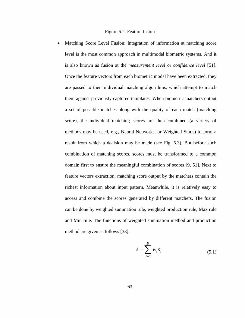
63
Figure 5.2 Feature fusion
• Matching Score Level Fusion: Integration of information at matching score
level is the most common approach in multimodal biometric systems. And it
is also known as fusion at the measurement level or confidence level [51].
Once the feature vectors from each biometric modal have been extracted, they
are passed to their individual matching algorithms, which attempt to match
them against previously captured templates. When biometric matchers output
a set of possible matches along with the quality of each match (matching
score), the individual matching scores are then combined (a variety of
methods may be used, e.g., Neural Networks, or Weighted Sums) to form a
result from which a decision may be made (see Fig. 5.3). But before such
combination of matching scores, scores must be transformed to a common
domain first to ensure the meaningful combination of scores [9, 51]. Next to
feature vectors extraction, matching score output by the matchers contain the
richest information about input pattern. Meanwhile, it is relatively easy to
access and combine the scores generated by different matchers. The fusion
can be done by weighted summation rule, weighted production rule, Max rule
and Min rule. The functions of weighted summation method and production
method are given as follows [33]:
∑=
=K
iii sws
1 (5.1)

64
∏=
=K
i
wi
iss1
)( (5.2)
where K is the modality number, wi the ith fusion weight, and si the ith score
obtained from the ith modality. A basic assumption of (5.2) is that scores from
different modalities are statistically independent; however this assumption is
unrealistic in many situations.
Figure 5.3 Matching score fusion
• Decision Level Fusion: Strictly speaking, decision level fusion is not a ‘truly’
fusion, although it is generally termed as such. The principle behind this
method is that each biometric system makes a match based solely upon the
biometrics it captures and then passes a binary “match/no-match” vector to a
decision module [56], which forms a conclusion based on a majority vote
scheme, AND, and OR operators. In majority voting, final decision is based
on the number of votes made by individual classifiers. However, it cannot be
done when there is an even number of sensors with the decisions made by half
of classifiers does not agree with the other half. AND rule is very strict and
therefore suitable only for systems that require low false acceptance; unlike

65
AND rule, the OR rule can make a decision as soon as one of the classifiers
make a decision. It is suitable for the systems that can tolerate a loose security
policy. Some systems also include a method to weight the decision towards
more highly regarded biometrics (e.g., iris over retina scans).
Figure 5.4 Decision fusion
Most observers accept that fusion produces better results when performed at feature
extraction level rather than at the data matching or decision levels, because the data is
combined at its most information rich stage and before external contamination from
matching algorithms. However, feature level fusion is difficult, as the relationship
between individual biometrics’ features spaces may not be straightforward [53]. The
problems associated with feature level fusion are noted in the literature [26], with most
fusion research being carried out in the data matching and decision level fusion areas.
5.3 Summary
Information fusion is a key issue in a multimodal biometric system, and it can
possibly take place in four levels, that is, sensor, feature extraction, matching score and
decision levels. Sensor level fusion is seldom used in commercial applications because of
compatibility problems. In other words, fusion at this level requires that the information
obtained from different multiple biometric sensors must be compatible, and that will be a

66
rare case with biometric sensors. Also, fusion at feature level is not always guaranteed
feasible, because the feature sets extracted from different biometric modalities may either
be inaccessible or incompatible to each other. Combination at matching score level is
easy to use in some degrees, and it has been researched and developed a lot since the
beginning of multimode biometric systems; meanwhile, it is easy to be used. The main
problem at this fusion level is to obtain the score weights of different modalities. Fusion
at decision level cannot represent the whole pictures of multimodal system, because only
a limited amount of information is available for fusion. Although multiple modal systems
can deal with the limitations of single modal systems and gain a lot of benefits, it should
be used with caution because catastrophic fusion may occur if biometrics is not properly
combined; such situations might happen if the results of fused strategies are worse than
those of any single modal revolved in the fused systems.

67
6 FUSION BY SYNCHRONIZATION OF FEATURE STREAMS
6.1 Introduction
Multiple modal biometrics systems, which use more than one biometrics modality
like retinas, irises, hand geometries, fingerprints, handwriting, audio and faces, have been
introduced in literature in chapter 2 to overcome the shortcomings of single modal
biometrics. And biometrics fusion, which integrates information from the applied
modalities and is implemented at several levels such as sensor fusion level, feature fusion
level, score fusion level, and decision fusion level, has becoming a critical issue in
multiple modal biometric systems.
Among the candidate modalities, both audio and face (visual) recognitions are
considered to be easy to use, and the low cost of audio and visual sensors also make it
feasible to deploy such audio-visual (AV) systems for surveillance, security, digital
libraries, forensic work, law enforcement, human computer intelligent interaction, and
smart environments etc. Moreover, in an AV system, the audio-based authentication part
can be classified into two categories: text-dependent and text-independent [3]. In a text-
dependent AV system, speakers must recite a phrase, password or numbers specified by
the system. This is in contrast to a text-independent system, where speakers can say
whatever they wish to say. That will give more freedom to the system and people.
Therefore, one of the principal advantages of a text-independent AV system is that it
allows the system to be applied to much more diversified tasks. For those reasons, this

68
chapter applies the proposed intuitive feature fusion methodology for multi-mode
biometric person recognition systems, especially concentrates on Audio-Visual based
Text-Independent (AVTI) system to test it in this chapter. Also, in the future chapters,
AVTI system is used as testing examples for other proposed optimized algorithms.
As stated before, in biometrics fusion, integrating information at an early stage, like
feature stage, is more effective than at later stages. Many works for multi-mode biometric
systems have been done so far. And some representative researches and studies have been
presented in Chapter 2 in details. But, the methods discussed in the literature in Chapter 2
include using lip movement or partial face images to represent visual cue in AV systems,
and almost all of them except Luettin [37] integrated multiple modal results in score or
decision fusion level. In Luettin’s work, lip movement from video streams and text-
dependent speeches were examined in the feature fusion level by concatenation with the
frame rate of the speeches.
This chapter introduces a novel person recognition approach. The testimony has
been done by using still face images and text-independent speech signals. In the proposed
method, the reason why the above two modalities are much more favorable to be used
than other modalities by the authors is that 1) still face images instead of video
information are considered to reduce storage space and computational complexity, and 2)
text-independent speech signals are used to allow AV systems more flexible for
diversified applications. Furthermore, both biometrics will be integrated at feature fusion
level by a novel synchronization method and exported to a PNN framework. A perfect
recognition rate has been achieved by applying the new feature fusion strategy to a virtual
database composed of 40 subjects.

69
The remaining of the chapter is organized as follows: Section 6.2 briefly reviews
feature extraction of AVTI system; Section 6.3 introduces the intuitive synchronization
method at feature level fusion; Section 6.4 examines this method; and the conclusion is
presented in Section 6.5.
6.2 Feature Extraction of AVTI system
As mention above, AVTI system in this chapter is different from other AV systems
in literature. The proposed methodology in AVTI system includes feature extractions
from visual images using the Pyramidal Gabor - Eigenface (PGE) algorithm [20] and
from audio signals using the Mel Frequency Cepstrum Coefficients (MFCCs) and Vector
Quantization (VQ) algorithms. The extracted features from both modalities are
normalized and fused to recognize the subjects under a PNN framework. Due to different
sampling rates used in the system, the extracted PGE features from still images should be
synchronized to fit the compressed audio features. For the continuity of this chapter and
the convenience of readers, the following will describe face and voice recognition in brief
respectively. For detail information, readers can go back to Chapter 3 & 4.
6.2.1 Audio feature extraction
One of popular methods for audio feature extraction is to apply MFCCs algorithm.
Such method is very straightforward. Several processing steps occur to obtain the audio
features in this chapter (see Fig. 6.1).

70
Figure 6.1 Procedures of MFCC
In Fig. 6.1, high-pass filter is used to enhance those high frequencies in signals that
are generally attenuated during recording process. After the procedures of Hamming
windowing, short-term speech segments with a length 20ms and an overlap of 10ms per
frame [3] are processed by Fast Fourier Transform and Mel-filter banks to get the Mel
spectrums. Then, discrete cosine transform (DCT) is applied to log of the filtered
frequency components to obtain Mel cepstrum. Considering the amount of feature sets
for each subject, Mel cepstrum has to be compressed by a VQ algorithm before being
fused in the proposed method.
6.2.2 Visual feature extraction
The visual features are extracted by the PGE algorithm [18, 20]. Such algorithm is
effective for person recognition because:
1) It utilizes 1-D filter masks instead of 2-D filter operation in spatial domain to
obtain Gabor features, which make it faster and more flexible with less
computational complexity than the classic Gabor-based recognition method
that needs to perform 2-D Fourier transform and inverse Fourier transform;
2) The Eigenface method further reduces the redundancy of Gabor features.
PGE algorithm consists of training and recognition stages. During training stage,
the features of training sets are obtained by applying the pyramidal Gabor wavelet
procedure [44] to training sets in four levels and four orientations (see 6.1 and 6.2). To
encompass the features of each training face image, the rows of all its feature
representations will derive an augmented feature representation via concatenation. Then,

71
the augmented feature representations for all training images are normalized to zero mean
and unit variance. Later, the Eigenface method [55] transforms them into the eigenspace.
The second stage of PGE algorithm uses equation (6.2) to extract the visual features
of testing face images, and projects the test difference vectors into eigenspace.
In the above procedure, Gabor function (6.1) of frequency f0, orientation θ0, and
centered at (x0 = 0, y0 = 0) is defined as a sum of two separable filters (see equation (6.2))
[20]:
))sincos(2exp(
))(exp(),(
000
222,,0,0 00
θθπ
πθ
⋅+⋅⋅
+−=
yxfj
yxayxg f
(6.1)
)]sin2sin([)]cos2sin([
)]sin2cos([)]cos2cos([),(
0000
00000,,,0,0 00
θπθπ
θπθπθ
yfgxfg
yfgxfgyxR
yx
yxpf
⋅⋅⋅−
⋅⋅⋅==
)]sin2sin([)]cos2cos([
)]sin2cos([)]cos2sin([),(
0000
00001,,,0,0 00
θπθπ
θπθπθ
yfgxfg
yfgxfgyxR
yx
yxpf
⋅⋅⋅−
⋅⋅⋅==
(6.2)
where gx and gy are 1-D Gaussian function )exp( 2axgx π−= and 01)/2ln3( fa −= π . Each block
in (6.2) is a 1-D filtering operation. By performing a constrained least squares
minimization of the error of frequency response [44], four 1-D Gabor masks can be
obtained. If θ0 is 00, 450, 900, 1350, respectively, these filters can be used to get the robust
Gabor features in four orientations and four levels.
6.3 Feature fusion
Biometric fusion is the critical part in any multi-modal biometrics system and there
are several level fusions. Among those levels, fusing information at feature stage is more
effective than at later stages. So far, some work about different AV systems has been
done to recognize persons via score or decision fusion. In this chapter, both biometrics in

72
AVTI system will be integrated at feature level by a novel synchronization method.
Before fusing the features extracted from different modalities, one should normalize them
to overcome the problems caused by different feature spaces, the variations in their
ranges and distributions of the individual feature vector values.
Meanwhile, synchronization is also important to an AV system. As an example,
given 128 compressed audio feature vectors and 6 PGE visual feature vectors for each
subject, every int(128/6) voice feature vectors will be concatenated with one identical
face feature vector: that is, duplicated visual feature frames are inserted to audio feature
vectors. Therefore, the compressed feature sets extracted from audio and visual signals
are synchronized by the way shown in Fig. 6.2, and then concatenated to obtain the new
augmented feature representations which are exported to the PNN framework.
Figure 6.2 Example of synchronization
PNN is a type of feed-forward neural networks with four layers: input layer, two
hidden layers, and output layer. It applies a standard Bayesian classifier and maps any

73
input pattern into a number of classifications without training because the conventional
training vectors simply become the weight vectors in the first hidden layer [48]. It
inherits the parallel structure that can be easily extended by adding new training samples
or removing the existed training samples. The activation function of a neuron in the PNN
framework of AVTI system is statistically derived from an estimation of probability
density functions (pdf
)(1)(σσ
kk
bzwzg −=
) based on the training data sets, and it can approximate the pdf of
the training subjects. The pdf of a given input pattern z belonging to one subject can be
estimated by
(6.3)
where z is the given input pattern, bk the kth pattern of subject C, w the evaluation
function, and σ the smoothing parameter.
The average value of pdf’s for the “M” patterns of subject C can be used as the
estimate of pdf for this subject:
)(1)(1
zgn
zh k
M
k∑=
=σ (6.4)
When Gaussian functions are used as the evaluation functions, the pdf of a given
input pattern z belonging to the kth pattern of one subject can be estimated by equation
(6.5), and the estimation of the pdf for a feature vector z belonging to subject Ci is given
by equation (6.6):
2
2,
2
||||
2/,)2(
1)( σ
σπ
ikbz
ppik ezg−−
= (6.5)

74
∑=
=M
kiki zgzh
1, )()( (6.6)
where k = 1, 2, …, M, i = 1, 2, … N, M the number of the feature vectors of
subject Ci; N the number of subject classes, p the length of z, σ the smoothing parameter,
bk,i the kth pattern of subject Ci.
Fig. 6.3 & 6.4 show the related architectures of PNN and AVTI system with feature
fusion. In Fig. 6.4, N denotes the number of persons in training data set; X is set as the
input of the PNN for a subject to be classified; AVi is the ith feature vector of X. The AV
patterns for each subject, resulted from the training stage, are used as the weights of its
first hidden layer. The outputs of each node of the first hidden layer are obtained using
(6.5). The summation layer adds all the estimates of the pdf for the feature vector X
belonging to subject Ci (i = 1, 2, …, N) with (6.6). The competitive network applies the
rule of “winner-take-all” to classify the input X using the following equation:
)},...,,({ 21 NhhhMAXINDI = (6.7)
where hi is from equation (6.6), MAX() and IND() denote max and index operations,
respectively.

75
Figure 6.3 PNN architecture
Figure 6.4 PNN structure for AVTI system.
6.4 Experiments
6.4.1 Experimental setup
A database including 40 subjects was constructed to test the proposed method. It
consisted of audio and visual parts. In audio part, a training set included text-independent
voices obtained by the same microphone from the public speeches of various topics in
noisy backgrounds; and a testing set with 40 voices of the same subjects also addressing
different topics. The lengths of audio segments for training and testing were 30 and 15
seconds, respectively. To take the temporal variation of speeches into the consideration,
the time interval between training and testing recordings was at least two weeks.
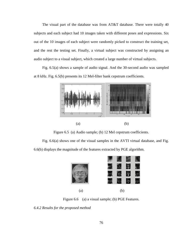
76
The visual part of the database was from AT&T database. There were totally 40
subjects and each subject had 10 images taken with different poses and expressions. Six
out of the 10 images of each subject were randomly picked to construct the training set,
and the rest the testing set. Finally, a virtual subject was constructed by assigning an
audio subject to a visual subject, which created a large number of virtual subjects.
Fig. 6.5(a) shows a sample of audio signal. And the 30-second audio was sampled
at 8 kHz. Fig. 6.5(b) presents its 12 Mel-filter bank cepstrum coefficients.
(a) (b)
Figure 6.5 (a) Audio sample; (b) 12 Mel cepstrum coefficients.
Fig. 6.6(a) shows one of the visual samples in the AVTI virtual database, and Fig.
6.6(b) displays the magnitude of the features extracted by PGE algorithm.
(a) (b)
Figure 6.6 (a) a visual sample; (b) PGE Features.
6.4.2 Results for the proposed method

77
In order to compare the performances from the proposed method and from the two
related single modal methods under the PNN framework, two experiments were
conducted. In experiment 1, it was chosen that, for each virtual subject, the length of the
audio signals was 25 seconds for training and 12.5 seconds for testing; and in experiment
2, 20 seconds for training and 10 seconds for testing. In both of the experiments, six face
images of each subject were employed for training and four remaining face images for
testing. In addition, the codebook size for VQ was initialized as 128. Furthermore, the
number of MFCC coefficients was set to 12.
Table 6.1 compares the results from the proposed AVTI recognition method and
from the two related single modal methods in the PNN framework. With the setup
described above, the proposed AVTI recognition system obtained the perfect recognition
rate of 100%. However, if only the audio-based features were used for human
identification, implemented with a similar PNN structure, the recognition rates were only
47.5% and 43.5%, respectively; and the recognition rate was improved to 96% by using
only the visual-based features. Such results suggest that the proposed method is clearly
worthy of further study.
Methods Recognition rate for best performance length of training audio (s) / length of testing audio (s)
25s / 12.5s 20s / 10s
Audio-based modal 47.5% 43.5%
Visual-based modal 96% 96%
Proposed method 100% 100%

78
Table 6.1 Comparison for various methods
The proposed method was also compared with the Minimum Distance (MD)
classification method, which was very simple and classified an object under a minimum
distance criterion of the fused features. The results in Table 6.2 indicate that AVTI
system under the framework of PNN performed much better than the MD method,
because MD method does not utilize statistical information for the fused features.
Table 6.2 Comparisons of the proposed method and MD method
Shown in Table 6.3 are the recognition rates vs. the lengths of AV feature vector.
Length of AV feature Recognition rate
25s / 12.5s 20s / 10s
22 90.0% 87.5%
24 90.0% 92.5%
26 92.5% 95.0%
28 97.5% 97.5%
31 100% 97.5%
32 97.5% 100%
Methods Recognition rate for the best performance (Length of training time (s) / length of testing time(s))
25s / 12.5s 20s / 10s
Proposed method 100% 100%
MD method 85% 87.5%

79
Table 6.3 Recognition rate vs. length of AV feature vector
The AV feature vector consisted of 12 MFCCs for the audio part and the first
several maximum PGE eigenvectors for the visual part. Table 6.3 shows that the perfect
recognition rate is achieved with the length of the feature vector being less than or equal
to 32. Among the 32 components, 12 were MFCCs, therefore, only at most 20 PGE
eigenvectors were needed to obtain the much better recognition rate in the AVTI person
recognition system. It demonstrates the proposed method has overcome the problem of
different frame rates from audio and visual signals and the curse of dimensionality in the
feature fusion procedure in some degrees.
6.5 Conclusion
A method for integrating audio and visual biometrics at feature level has been
presented in this chapter. The described framework can synchronize the compressed
visual and audio features to form a mixed feature space efficiently. It has been shown
through experimental studies that the integrated method to the AVTI system at fusion of
feature level can achieve superior performance in comparison to any of the individual
biometrics it derives. In addition, since only still images are needed for the
implementation of the approach, the storage space and process time can be more
economical compared to techniques based on integrating video with audio information.
The testing results of the AV system also indicate that the proposed algorithm overcomes
the problem of different frame rates from the audio and visual signals and the curse of
dimensionality normally existed in a feature fusion procedure.

80
7 FUSION BY LINK MATRIX ALGORITHM AT FEATURE LEVEL
7.1 Introduction
Biometric identification and authentication systems can be classified as single
modal systems and multiple modal systems. As stated before, although single modal
system has been shown to be effective and robust under certain conditions, system
performance degrades in the presence of sensory noise and mismatch between training
and testing environments. In order to overcome its shortcomings, various multiple modal
systems, which use more than one modality at a time, have been addressed in the
literature in chapter 2. Moreover, choice of biometric modalities depends on factors such
as accuracy, robustness, sensor size and cost.
The goal of this chapter is to devise an effective method to integrate biometric
information from multiple modals, as an example, audio and visual (AV) biometric
modalities have been applied to implement and test the proposed methodology at feature
level. Of course, depending on different types of audio and visual signals used, AV
systems can be any of the followings: visual-static text-dependent speech, visual-static
text-independent speech, visual-dynamic text-dependent speech, and visual-dynamic text-
independent speech systems. In this chapter, visual-static text-independent speech bi-
modal system is employed as the specific AV system.
There exist many fusion methods in the studies of multiple modal biometrics;
methods for AV systems listed in Chapter 2 have been almost exclusively focused on

81
using either lip movement or video to represent visual cues and integrate multiple cues
by score fusion and/or decision fusion. Investigators have seldom studied biometric
fusion at feature level because there are some difficult issues, especially for AV feature
fusion. But, there appears to be a consensus [20, 33] that integrating information at
feature level is more effective than doing so at higher levels. Therefore, feature level
fusion should be taken a shot. However, before fusing features from audio and visual
signals, audio and visual feature streams have to be synchronized, and this may lead to a
high dimensionality, that is a very bad news to the fusion algorithms. In order to fuse the
information from multiple modalities effectively, this chapter apply the proposed method
to combine feature vectors (see Fig. 7.1). Cost function, constraints and possible
simplifications are outlined. A heuristic algorithm which is suitable for biometric
applications is proposed. Once audio and visual features are combined to form an
integrated feature vector, they are fed to a block similar to Radial Basis Functions (RBF)
[7] to perform classification. Experiments are carried out for 40 subjects from a virtual
database consisting of face images and speech clips. The results show that 1) the
proposed method performs better than those without fusion, and 2) it is more reasonable
than the one in Chapter 6.

82
Figure 7.1 Procedures of the proposed feature fusion method
The remainder of this chapter is organized as follows: Section 7.2 provides some
preliminaries and Section 7.3 proposes a fusion method for integrating features from two
biometric sources. In Section 7.4, a classification method is proposed which is similar to
RBF that analyzes the probability density functions (pdfs) of the feature vectors. Some
results from experimental studies are presented and discussed in Section 7.5 and the
chapter ends with concluding remarks in Section 7.6.
7.2 Preliminaries
In any person recognition system, feature extraction of individual modality is one of
the most essential steps, because the performance of systems strongly relies on the
accurate extraction of biometric features. When considering audio feature extraction for
speaker recognition, in theory, it should be possible to recognize speakers directly from
waveforms. Because of the large variability of speech signals, it is, however, a good idea
to extract essential features from speech signals. This is also true for face recognition.
Thus, feature level fusion is an attractive approach, which is the main reason that we
focus on feature based biometric fusion. Some basic concepts and algorithms are briefly
stated here for completeness.
In the AV system under investigation, visual and audio features are extracted by
pyramidal Gabor wavelet with eigenface (PGE) algorithm [20] and Mel Frequency
Cepstrum Coefficients (MFCCs) algorithm [3], respectively.
In PGE algorithm, involvement of Gabor wavelets benefits face recognition and
makes it more robust against variations from lighting condition and viewing direction. In
addition, to save computational cost and memory space, a pyramidal structure is used in

83
spatial domain to avoid the procedures of Fourier transform and inversed Fourier
transform, which are often utilized in general 2-D Gabor based face recognition methods.
The central task of a typical audio-based feature extraction procedure is to
parameterize speech signals into a sequence of feature vectors that are less redundant for
statistical modeling. Spectral features, such as Linear Predictive Cepstrum Coefficients
(LPCCs) or Mel Frequency Cepstrum Coefficients (MFCCs) have been widely used [3].
In this section, the procedure of MFCCs is also outlined. The above feature extraction
methods have been discussed in Chapter 4 and 5 in details. For the relevant information,
please go back and read those chapters.
7.3 A method to fuse features
In this section, biometric information fusion is formulated as an optimization
problem. Cost function, constraints and solution strategies are discussed with a simple
example. The method developed is then applied to fuse audio and visual feature vectors.
Given feature vectors from two sources, the task is to combine them so as to
optimize certain performance criteria, such as computational cost and accuracy. We use
a simple example to illustrate the essence of the proposed method. Suppose that two
modalities, M1 and M2, are used in individual biometric algorithms. Suppose also that the
ith subject Si in modality M1 and M2 has 3 and 5 components, respectively, a component
{a1i, a2i, a3i} belongs to the ith subject Si in modality M1, and components {v1i, v2i, v3i, v4i,
v5i} belong to Si in modality M2. We can then define a 5x3 Link Matrix B, whose entries
are either 1 or 0, with 1 denoting a pair of variables (or vectors) selected to form a new
vector from an individual modality. For instance, if b12 = 1, where bij is the ijth entry of
B, then v1i and a2i are selected to be part of a feature vector in the form of [v1i a2i]T.

84
To further illustrate the idea, let us use equation (7.1) as an example. The first row
of the B matrix [1 0 0] in (7.1) means that the first feature component v1i of subject Si in
modality M2 joins the first feature vector a1i of subject Si in modality M1. The second row
of the B matrix [0 1 0] implies that the second feature vector v2i of subject Si in modality
M2 joins the second feature vector a2i of subject Si in modality M1. Going through all the
rows, the matrix B given in (7.1) implies that an Integrated Feature Vector qi = [v1i a1i v2i
a2i v3i a1i v4i a3i v5i a2i] T is obtained, given individual biometric vectors [v1i v2i v3 v4i v5i] T
and [a1 a2i a3i] T. This Integrated Feature Vector will then be fed to a classification
algorithm for further biometric authentication/identification.
=
010100001010001
B (7.1)
Graphically, the relationship specified by (7.1) can be illustrated by the diagram
shown in Fig. 2.
Figure 7.2 Illustration of Link Matrix B between modality M1 and M2.
With the Link Matrix B defined, we can formulate the problem of combining
features from two biometric sources in terms of Link Matrix selection. Let us generalize
the notation used in the previous example as follows:
1 2 3 4 5
1 2 3
M2 M1

85
• aij: the ith component of subject Sj in modality M1, where i = 1,…, m; m is the
number of components in M1. Note that aij can be a vector.
• vkj: the kth component of subject Sj in modality M2, where k = 1,…, n; n is the
number of components in M2.
• bik: the entry of matrix B in ith row and kth column. Further, ]1,0[∈ikb , where bik
= 1 if aij in M1 joins vkj in M2; otherwise, bik = 0.
Let us now define an error function, E, against which the accuracy performance of a
biometric identification/authentication algorithm is to be judged. We desire a structure
for B that is as simple as possible to reduce the computational cost. These and other
objectives are summarized next.
1) It is desirable that the error function be minimized; i.e.,
)()(1 BEBQ = , (7.2)
2) It is also desirable that the length of the Integrated Feature Vector be
minimized. This is equivalent to minimizing Q1, where
1)(0 1 12 ≤
∗=<∑∑= =
nm
bBQ
m
i
n
kik
, (7.3)
3) Each component in modality M1 and M2 appears at least once in the Integrated
Feature Vector; i.e.
31
41
1
1,
n
i ikkm
i iki
Q b
Q b
=
=
= ≥
= ≥
∑
∑ (7.4)
where i = 1, …, m; k = 1, …, n.

86
Taking into consideration the above factors, the optimization problem is equivalent
to minimizing the following objective function by choosing the Link Matrix B,
))()()( 2 BQBEBC λ+= , (7.5)
subject to (7.4), where 10 ≤≤ λ .
Assume that mn > , set Q3i to 1; that is
1
,1
14
13
≥=
==
∑
∑
=
=
m
iiki
n
kiki
bQ
bQ (7.6)
In this case, each component of the given subject in modality M2 is guaranteed to be
picked up once and only once to form the Integrated Feature Vector. Note that whenever
this occurs, Q2 becomes a fixed number and objective function; therefore,
)()( BEBC = (7.7)
Mathematically the case in which m > n, Q3i ≥ 1 and Q4i = 1 can be treated
similarly to that given by (7.6) and (7.7).
The following remarks can be made about the solutions of the proposed problem:
• An exhaustive search [30] works fine with simple problems having relatively
low dimensionality. Such a solution examines all possible choices of the Link
Matrix B and the associated objective function values. This may not be a
viable solution when the size of the problem becomes large.
• Blind random search [30] over the domain of interest is a method aimed at
reaching an acceptable solution. The eventual solution is obtained simply by
taking the choice of B that yields the lowest C value among the randomly
tested candidate solutions.

87
• Heuristic search [30] is another method that exploring the structure of the
solution space and guiding the search directions. This approach may not
always find the best result, but normally efficiently finds a near-optimal
solution.
A simple search procedure is proposed in this chapter to obtain a sub-optimal
solution. In each iteration, a configuration of B is randomly generated. If the solution
results in a better value of the objective function, it will be kept and set as the current
chosen solution; otherwise, it will be ignored. The following steps are applied to obtain
the Link Matrix B:
1) Randomly generate a matrix B that satisfies (7.4) (or (7.6));
2) Compute the objective function C with the matrix B using (7.5) (or (7.7));
3) Save both matrix B and result C, and set B as Bbest and C as Cbest,
regarding Bbest as the current solution;
4) Randomly generate another matrix B that satisfies (7.4) (or (7.6));
5) Evaluate the objective function C using (7.5) (or (7.7)) with the new
matrix B obtained in Step 4:
a) If C is better than Cbest, replace Bbest with the new B and update Cbest.
b) Otherwise, just ignore the new solution.
6) Iterate the steps 4) and 5) till either the error C is below a preset tolerance
or the maximum number of iterations is reached.
7.4 Case Studies
A simple example is given here to illustrate the method proposed above. In this
example, we assume that there are three subjects S1, S2 and S3, and each subject has two

88
modalities to represent it: the shape modality M1 and color modality M2. In modality M1,
three patterns of each subject are assumed to be the training data set and the fourth is
assigned as the testing data set. In modality M2, six patterns of each subject are assumed
to be the training data set, and another six are assigned as the testing data set. In addition,
data streams consisting of 1 and 0 represent each pattern in M1 and M2. Fig.7.6 and Table
7.2 show the patterns of three subjects S1, S2 and S3 in modality M1 and M2, respectively.
Figure 7.3 Patterns for subject S1, S2 and S3 in modality M1, respectively
Using the method given in Section III.A, a Link Matrix B, obtained using (7.6)
and (7.7), is shown in Equation (7.8). With this Link Matrix, a perfect classification
is obtained.
1 1 1 1 1 0 0 0 1 0 0 0 1 0 0 0
1 1 1 1 0 0 0 1 0 0 0 1 0 0 0 1
1 0 0 0 1 0 0 0 1 0 0 0 1 1 1 1
0 0 0 1 0 0 0 1 0 0 0 1 1 1 1 1
0 0 0 1 1 1 1 1 0 0 0 1 0 0 0 1
0 0 1 0 0 0 1 0
0 0 1 0 1 1 1 1
1 0 0 0 1 0 0 0 1 1 1 1 1 0 0 0
1 1 1 1 0 1 0 0 0 1 0 0 0 1 0 0
1 1 1 1 0 0 0 1 0 0 0 1 1 1 1 1
1 1 1 1 1 0 0 0 1 0 0 0 1 1 1 1
1 1 1 1 1 0 0 1 1 0 0 1 1 0 0 1
1 0 0 1 1 0 0
1 0 0 1 1 1 1 1
S1
S2
S3
Training set Testing set

89
Table 7.1 Patterns for subject S1, S2 and S3 in modality M2
Training set Testing set
Patterns for S1
1 0 0 0 0 0 1 0 0 0 0 0
0 1 0 0 0 0 0 1 0 0 0 0
0 0 1 0 0 0 0 0 1 0 0 0
0 0 0 1 0 0 0 0 0 0 1 0
0 0 0 0 1 0 0 0 0 1 0 0
0 0 0 0 0 1 0 0 0 0 0 1
Patterns for S2
1 0 1 0 0 0 0 0 1 0 1 0
0 1 0 1 0 0 0 1 0 1 0 0
0 0 1 0 1 0 1 0 1 0 0 0
0 0 0 1 0 1 0 0 0 1 0 1
0 0 0 1 0 1 0 1 0 1 0 0
1 0 1 0 0 0 0 0 0 1 0 0
Patterns for S3
1 1 0 0 0 0 0 0 1 1 0 0
0 0 1 1 0 0 0 0 0 0 1 1
0 0 0 1 1 0 0 1 1 0 0 0
0 0 0 0 1 1 0 0 0 1 1 0
0 0 1 1 0 0 0 1 1 0 0 0
0 1 1 0 0 0 0 1 0 1 0 0

90
=
010100100001001100
B (7.8)
7.5 Proposed Classification Method
After features from both audio and visual signals are integrated, another factor
affecting system accuracy is the choice of classification method. Classification attempts
to assign a measurement to a class or identify the source of a measurement. Some popular
methods include least-squares, maximum-likelihood, Bayesian, Hidden Markov Models,
and artificial neural networks. In this section, together with the least-squares method, a
RBF-like [7] method is presented, which is based on analyzing probability density
functions (pdfs) of the integrated feature vector.
7.5.1 AV identification based on least-squares algorithm
One of simplest classification methods is the least-squares (LS) algorithm, which
classifies an object under a minimum distance criterion. Consider the case of
classification in an AV system. Let us assume that ,,, 21 yy and ny are n feature vectors
in the database and denote z the feature vector representing the subject under test. The
LS method solves the following problem:
2min zyii− (7.9)
Although the LS method is very simple, its results are expected to be worse than
those obtained by methods utilizing statistical information.
7.5.2 AV identification based on analyzing pdfs

91
Another method adopted in this chapter utilizes the pdfs of feature vectors. The pdf
of a given input pattern x belonging to a subject may be represented by
)(1)(σσ
kk
xxWxg −= (7.10)
where x is a given input pattern, xk the kth pattern of subject C, W a distribution
function, and σ a smoothing parameter. The average value of the pdfs for the “n” patterns
of subject C can be used as the estimation of the pdf for this subject:
)(1)(1
xgn
xG k
n
k∑=
=σ
(7.11)
When Radial Basis Functions [7] are utilized as distribution functions, the pdf of a
given input pattern x belonging to the kth pattern of one subject can be estimated by
(7.12), and the estimation of the pdf for x belonging to subject Ci is given by (7.13):
2
2,
2
||||
2/, )2(1)( σ
σπ
ikxx
ppik exg−−
= (7.12)
∑=
=n
kiki xgxG
1, )()( , (7.13)
where k = 1, 2, …, n, i = 1, 2, … N; n is the number of feature vectors of subject
Ci; N the number of subject classes; p the length of x; and xk,i the kth pattern of subject Ci.
The input x is classified by using the following equation:
)},...,,{max( 21 NGGGindI = , (7.14)
where max() and ind() denote max and index operations, respectively. If the objective is
to identify a subject that includes several patterns, the classification is defined by.
))}({max( IhistindR = (7.15)

92
7.6 Experimental studies
In this section, several experiments were implemented to test the proposed methods
with a database of 40 virtual subjects. After analyzing the pdfs of the fused feature
vectors, test results were obtained for single modal and multi-modal systems, both of
which are detailed in the sequel.
7.6.1 Experiment setup
To test the proposed approach, an audio and visual text-independent person
recognition database was constructed. The virtual database is setup like the one in
Chapter 6. For detail, please go back to read Section 6.5 in Chapter 6.
In order to compare the performance of the proposed method with that of two related
single modal methods, two experiments were conducted. In these experiments, it was
decided that, for each virtual subject, the length of the audio signals was 25 seconds and
20 seconds for training and 12.5 seconds and 10 seconds for testing, respectively. In
addition, the codebook size for VQ was initialized to 128. Furthermore, the number of
MFCC coefficients was set to 12. The following tests were conducted to evaluate the
effectiveness of the proposed approach:
• LS vs. RBF-liked classification
• Robustness of the proposed method
7.6.2 LS vs. RBF-liked classification
The RBF-like method was compared with the LS method. The results presented in
Table 7.2 indicate that the former performed much better than the latter, as the RBF-like
method incorporated statistical information for classification.

93
Approach AV recognition rates for best performance (Length of training time(s) / length of testing time (s))
25s / 12.5s 20s / 10s
LS-based 85.0% 87.5%
RBF-like 100% 100%
Table 7.2 LS vs. RBF-like classification
7.6.3 Robustness of the proposed method
It was shown in [18, 19, 21, 22] that the sub-system based on the visual modality
outperformed the one based on the audio modality. In this experiment study, we would
check the robustness of the proposed approach by feeding the algorithm with lower
resolution photos and de-noised audio signals. The RBF-like classification method was
employed in the system to identify the subjects under test.
As to the visual data, the resolution of face images in AV database is decreased by
4, 8 and 16 times, respectively. Moreover, audio signals were de-noised before feature
extraction to increase the recognition rate, because noise affected the performance of
audio-based systems. In visual sessions 1 and 2, different photos were used. In both
cases, however, the lengths of audio segment for training and testing were 25s and 12.5s,
respectively. The number of MFCC coefficients was set to 12. Fig. 7.5 shows the images
whose effective resolution [40] was reduced by 2 and 4 times, respectively. Table 7.3[21,
59] presents a comparison of the results obtained by different approaches.

94
(a) Original image. (b) Image downgraded by 2. (c) Image downgraded by 4
Figure 7.4 Examples for reducing the effective resolution.
Visual Session 1 Visual Session 2
Approach Recognition rate Approach Recognition rate
LS Proposed LS Proposed
AV Original 85% 100% AV Original 87.5% 100%
Down 4 75% 100% Down 4 75% 100%
Down16 60% 93% Down16 62.5% 94%
Visual
only
Original 96% Visual
only
Original 98.5%
Down 4 90% Down 4 93.5%
Down16 71.3% Down16 71.5%
Audio only 67.5% Audio only 67.5%
Table 7.3 Comparison result under various conditions
From this table, the recognition rates of visual-based person recognition system
were downgraded by reducing the effective resolution of the images. Without changing
resolution, recognition rates for Session 1 and 2 were 96% and 98.5%, respectively. After
image resolution was down by 4 and 16, the performance of the visual-based system was
dramatically worsened, but the proposed integrated system still performed well.
From the above table, when the image resolution was down by a factor of 16, the
recognition rates by using only visual data were about 71%. The rate for audio only was
about 68%. The difference between them was about 3%. Both of the sub-systems

95
performed poorly under the condition. However, the proposed integrated AV system
(fused at the feature level) achieved at least the recognition rate of 90%.
Furthermore, the proposed method based on RBF-like classification was compared
with the LS method. The results in Table 6 show that the former performed much better
than the later with (93-94% vs. 60-62.5%) when the visual data was greatly corrupted.
7.7 Conclusion
In this chapter, a new feature fusion method is proposed for the integration of any
bi-modal biometric data and applied to a person recognition system utilizing photos and
text-independent speech signals. An RBF-like classification method has also been
introduced for the problem under consideration. In order to test the efficiencies of the
approach presented in the chapter, different experiments were carried out. The results
obtained from these experiments revealed that integrating information at the feature level
by the proposed method achieved superior performance in comparison with any of the
single modal systems from which it is derived. The proposed feature fusion method also
produced measurable performance gains compared to methods based on intuition. Future
studies include the development of algorithms that can efficiently produce a Link Matrix
in an optimal sense.

96
8 FUSION BY GENETIC ALGORITHM AT FEATURE LEVEL
8.1 Introduction
Biometric system, both single modal and multiple modal systems, has been widely
used in many applications. To solve some problems of single modal systems, various
multiple modal systems have been proposed and addressed in the literature. Meanwhile,
multiple modal systems have their own issues which have to be concerned in
applications, for example, how to choose biometric modalities and how to effectively
integrate information of the biometrics involved in systems.
As we have known, biometric traits can be integrated at the levels of sensor,
feature, score and decision. Sensor fusion combines the raw data from multiple biometric
sensors to generate new data from which features can be extracted; matching score level
combines scores from biometrics involved to determine the identities of subjects;
decision level employs majority voting or OR rules to reach the final verdict; feature
level will concatenate features from all the modalities involved to form an integrated
feature vector with a higher dimensionality that represents a subject’s identity in a new
hyperspace. Among those fusions, feature level is expected to perform better. However, it
is difficult to implement as features from multiple biometric sources may not be
compatible, and even if they are compatible, there is still an issue of how to effectively
fuse features. The literature review has been presented in Chapter 2. For details, please go
back to check the survey in that chapter.

97
The goal of this chapter is to devise another effective method to integrate
information from two or more biometric sources. In order to test the efficiency of the
proposed technique, visual-static images and text-independent speech clips are integrated
with the method at feature level fusion in the experimental study for person recognition.
Fig. 8.1 shows the procedures of integrating biometric information of biometric A
and biometric B in several fusion levels. Especially, the general framework for feature
level fusion is specified in detail in Fig. 8.2. There exist different algorithms for the
procedures of feature fusion and classification. In Fig. 8.2, the algorithms for feature
fusion procedure can be genetic algorithm (GA) [59] and tabu search (TS), etc. Also,
some classification methods can be employed such as least square (LS), weighted least
square (WLS) [7] and probability neural network (PNN) methods.
Figure 8.1 Fusion of biometric A and biometric B at various levels

98
Figure 8.2 General framework for feature level fusion
In this chapter, feature fusion problem is formulated as an optimization one first. It
is a more optimized algorithm to the ones in Chapter 6 & 7. As a solution strategy, GA is
proposed to find its optimal solution [59], though in this case, other optimization
algorithms may be as efficient as GA is. As a case study, the proposed approach is
applied to integrate feature data from a virtual AV system.
The remainder of the chapter is organized as follows: Section 8.2 discusses fusion
method along with GA algorithm. The idea is illustrated by integrating features from two
biometric sources. Some results from experimental studies are presented and discussed in
Section 8.3, and the chapter ends with concluding remarks in Section 8.4.
8.2 Proposed GA fusion method
In this section, the cost function, constraints and solution strategies are discussed.
Assuming that each subject’s feature vectors are extracted and normalized from M
sources: D1, D2… and DM, the task is to combine them so as to optimize certain
performance criteria, such as computational cost and accuracy. The notations used are
defined below:

99
M: number of modalities.
Di: the ith modality, where ],......,2,1[ Mi∈ .
Ni: number of features in modality iD .
Pij: the jth component in the ith normalized feature type.
ijα : weight for the jth component in the ith feature type.
The objective for information fusion from M modalities is to obtain best
performance by choosing the right weights, ijα , to each feature in different modalities:
]..............[ 221122222221211112121111 2211
TMNMN
TMM
TMM
TNN
TTTNN
TTMM
PPPPPPPPP ααααααααα (8.1)
The weights of the one of feature types can be set to 1. As an example, suppose that
there are two types of modalities in the systems, and the features in each type are equally
weighted. In this case,
1......
......
222221
111211
2
1
=====
====
αααα
αααα
N
N (8.2)
One can then select 1 such that a performance measure is optimized. Once 1 is
obtained, the integrated feature vector is then
]............[21 2222111121111
TN
TTTN
TT PPPPPP ααα (8.3)
The following remarks can be made about the solutions of the proposed problem:
• Random search is a method aimed at reaching an acceptable solution. The
eventual solution is obtained simply by taking the choice of ijα that is used to
fuse the information and yields the best performance of the multimode system

100
among the randomly tested candidate solutions. Such a strategy may take a long
time to achieve the suitable weights ijα for the system.
• Gradient search is probably the easiest way to find the extreme. Visually the
strategy of a gradient search is to pick the direction that is steepest uphill (or
downhill) from the guess, and move in that direction until the graph levels out.
Mathematically, in each step, the gradient is used as the direction of search. The
process is repeated until the gradient approaches zero. Therefore, such a method
attempts only to find a local maximum or minimum.
• Genetic algorithm (GA) [59] is a search technique for seeking optimal solutions.
It is based on the principle of natural selection to simulate the search problem.
The search starts with a randomly generated initial population. At each step, the
algorithm selects individuals randomly from the current population to be parents
to produce children for the next generation. Over successive generations, the
population will evolve toward one containing the optimal one.
GA is employed in this chapter to find the optimal solution for biometric fusion
problem, and there are several building blocks in GA: initialization, selection,
reproduction and termination. Initially a set of individual solutions are randomly
generated to form the initial population, whose size typically contains hundreds of
possible solutions and covers a wide range of the search space. During each successive
generation, a new generation is bred after selecting a portion of the existing population
with a fitness function, which rates the fitness of each solution and preferentially selects
the better individuals. Roulette wheel selection is one of well-studied methods. Its fitness

101
level is used to associate a probability of selection with each individual chromosome. If fi
is the fitness of individual i in the population, its probability of being selected is,
∑=
=N
jj
ii
f
fp
1
(8.4)
where N is the number of individuals in the population.
Crossovers and mutation are employed to generate children from “parents” selected
for mating with the procedure [59] similar with the one outlined above. A new solution is
created which typically shares many of the characteristics of its "parents". Such process
continues until a new population of solutions of appropriate size is generated.
The following steps illustrate the core of GA algorithm [59]:
Step 1: Randomly choose the initial population;
Step 2: Evaluate the fitness of each individual in the population;
Step 3: Repeat the following until a new population is generated:
1) Select individuals based on, say, Roulette wheel procedure;
2) Breed new generation by applying crossover and mutation;
Step 4: Repeat Steps 2 and 3 until the solution is not improved more.
There exists a variety of variations to the procedure outlined above. Two-point
crossover algorithm creates two children by exchanging genes of pairs of parents in the
current population. Occasional mutation makes small random changes to the individuals
in the population. Meanwhile, a way to speed up the convergence of the algorithm is to
keep a number of the best solutions from one generation to another. Another way of

102
speeding up is to have a set of initial guesses based on the physical constraints of the
problem. For fusion, the following steps are applied to obtain the weights ijα :
Step 1: Assumed the information vectors are equally weighted within any one type
of modalities;
MiforiiNii i,......,2,1......21 ===== αααα (8.5)
where i is for the ith modality, Ni is the number of information vectors in the
ith modality Di, which are to be fused with others from other modalities.
Step 2: Use iα to be the center of the ranges for unknown ijα and apply the GA
algorithm to find ijα .
iiijii DD +≤≤− ααα (8.6)
where threshold Di is given according to experiments, and Mi ,......,2,1= .
In Step 1, the values may be determined by a simple optimization procedure as the
number of parameters involved in this stage is relatively much smaller. Furthermore, if
only two modalities are involved, one unknown 1α needs to be determined in this step. In
such a case, the Golden Ratio method, which is very efficient for such an application, can
be applied to find the value of 1.
In the case of feature level fusion, once the fused feature vectors are obtained with
the proposed method, these will be used for classification (Figure 1). Among various
classification methods, Probability Neural Network (PNN) and Weighted Least-Square
(WLS) algorithm are viable candidates.

103
The activation function in PNN is derived from an estimation of probability density
functions (pdf) based on a set of training set. The pdf of input x belonging to subject Ci
can be estimated by (8.7) and classified by (8.8):
2
2
2||||
2/)2(1)( σ
σπ
ixx
ppi exg−−
= (8.7)
))(( xgnimind ii
= (8.8)
where i = 1, 2, … N, N the number of subject classes, p is the length of x, σ the
smoothing parameter, x,i the pattern of subject Ci.
Least square method is used to compute estimations of parameters and to fit a set of
data. There exist several variations, and a more sophisticated version is WLS, which
often performs better because it can emphasize the importance of each observation [7].
The idea is to assign to each observation a weight that reflects the uncertainty of the
measurement. The error vectors ∆Fi in WLS can be defined as
jjj xff −=∆ (8.9)
[ ]Mi ffF ∆∆=∆ ,,1 (8.10)
where fj is the feature of training subjects, xj is the jth feature vector representing the
subject under test, j = 1, 2, … M, and M is the number of feature vectors for each subject.
Furthermore, i = 1, 2 … N, where N is the number of subject classes. Let the
weights [ ]Mββββ ,,, 21 = , the objective function can be defined as
( ) ( )iT
iiFF ∆∗∆∗ ββmin (8.11)
Let

104
=Γ2
21
0
0
Mβ
β
(8.12)
Then (8.11) is rewritten as
( ) ( )iT
iiFF ∆Γ∆min (8.13)
In experiments, we find that PNN produces similar results to WLS. However, the
WLS algorithm does not suffer as much the problem of “curse of dimensionality”, in
comparison to PNN. Also, WLS algorithm is much simpler to implement.
8.3 AV Case Studies
An AV system using the proposed method is shown in Fig.8.3. The database
consisted of the audio part and face (visual) part with 40 subjects. The virtual database in
these experiments is setup as the one in Chapter 6 & 7. For details, please check the
previous chapters.
After audio and visual data were fused using GA, the integrated feature vectors
were fed to PNN or WLS to produce test results. For a comparison study, results from
both single and multiple modal systems are detailed next.

105
Figure 8.3 AV feature level fusion
In order to compare the performance of the proposed method with that of the two
related single modal methods, several experiments were conducted. In these experiments,
it was decided that, for each virtual subject, the length of the audio signals was 25
seconds for training and 12.5 seconds for testing, respectively. In addition, the codebook
size for VQ was initialized to 128. Furthermore, the number of MFCC coefficients was
set to 12. In the GA algorithm, the two-point crossover method was used with crossover
rate 0.8, the elite size was 2, and the mutation rate was set as 0.002.
From Table 8.1, the best performances of PGE method were 96.0% and 98.5% for
original data session 1 and 2, respectively. These results indicate that PGE was very
suitable for recognizing persons. The Gabor wavelet representation facilitates recognition
without correspondence in the PGE algorithm, because it captures the local structure
corresponding to spatial frequency, spatial localization, and orientation selectivity.
Also, shown in Table 8.1 are some testing results for text-independent audio-based
single modal person recognition. The experimental result suggested that the recognition
rate was improved from 47.5% to 67.5% after audio signals for both testing and training
were de-noised. This is expected, as the performance of speaker recognition heavily relies
on the clearness of audio signals, and the de-noising procedure reduces the deleterious
effect of background noise.
The proposed fusion method was compared with the single modal systems under
the classification methods of the PNN and WLS algorithms. The results from the PNN
and WLS methods were identical, which was expected. Thus, in the subsequent
experiments, we used the WLS method to classify the fused features of visual and audio

106
signals. And in training visual session 1, the maximum value for the dimension of the
fused feature for one subject was M, where M = 128x12+6x239 = 2970 when all of the
eigenvectors for visual features have been employed. The results presented in Table 8.2
indicate that the former performed much better than the latter.
It was shown the sub-system based on the visual modality outperformed the one
based on the audio modality in [19, 21, 22, 24]. In this experiment study, we would also
check the robustness of the proposed approach by feeding the algorithm with lower
resolution photos and de-noised audio signals in order to obtain closer recognition results
from both of the single modal systems.
As to the visual data, the resolution of face images in AV database is decreased by
4 and 8 times, respectively. Moreover, audio signals were de-noised before feature
extraction to increase the recognition rate, because noise affected the performance of
audio-based systems. In visual sessions 1 and 2, different photos were used. In both
cases, however, the lengths of audio segment for training and testing were 25s and 12.5s,
respectively. The number of MFCC coefficients was set to 12. Table 8.1 presents a
comparison of the results obtained by different approaches.

107
Table 8.1 Comparison result under various conditions
From this table, the recognition rates of visual-based system were downgraded by
reducing the effective resolution of images. Without changing the resolution, recognition
rates for Session 1 and 2 were 96% and 98.5%, respectively. After image resolution was
down by 4 and 8, the performance of the visual-based system was dramatically worsened
to 90% and 81.3% for visual session 1 and to 93.5% and 83.0% for visual session 2,
respectively; however the proposed integrated AV system still performed well.
Because the single modal recognition system with face only information performed
much better than the voice only modal system, the features from the visual part will gain
more weight than those from audio part in the AV system. In the tests performed in this
section, weights for the audio part were assumed to be equal to 1, which only leaves the
Visual session 1 Visual session 2
Approach Recognition rates Approach Recognition rates
AV fusion Original visual 100% AV
fusion
Original visual 100%
Down 4 visual 100% Down 4 visual 100%
Down 8 visual 97.5% Down 8 visual 97.5%
Visual
only
Original visual 96.0% Visual
only
Original visual 98.5%
Down 4 visual 90.0% Down 4 visual 93.5%
Down 8 visual 81.3% Down 8 visual 83.0%
Audio
only
Original audio 47.5%
Denoised
audio
67.5%

108
weights for the visual part remaining unknown. After employing golden ratio method, the
initial values of α2 for visual parts are obtained and listed in Table 8.2. Meanwhile, each
individual feature has a different influence in person recognition. After applying GA
method to search the parameters, the weights for visual features were obtained for the
integration of the features extracted from visual and audio signals (Table 8.2). This
illustrates the relative importance of each coefficient in person recognition.
α2 α21 α22 α23 α24 α25 α26
Original 22.01 23.6742 22.6813 22.0118 22.0307 23.9000 20.8905
Down 4 21.18 20.5679 20.2311 21.4008 23.5144 21.2964 21.1230
Down 8 21.80 22.4153 23.7919 22.7807 21.6588 20.4468 20.2479
Table 8.2 Weights for visual part in the virtual AV system
8.4 Conclusion
In this chapter, a feature fusion method is proposed for the integration of multi-
modal biometric data, and as a special case, it is applied to a person recognition system
utilizing photos and text-independent speech signals. The weights of individual feature
vectors are obtained with a GA algorithm and subsequently used in a classification
procedure for person recognition. In order to test the effectiveness of the proposed
approach, a number of experiments were carried out. The results obtained from these
experiments revealed that integrating information through the proposed method achieved
much better performance and maintained much more robust results in comparison with
any of the single modal systems from which it was derived.

109
9 FUSION BY SIMULATED ANNEALING AT FEATURE LEVEL
9.1 Introduction
Biometric systems have been attracted the attention from the public because of
some high profile applications, such as FBI Integrated Automated Fingerprint
Identification Systems (IAFIS), Criminal Scene Investigation (CSI) science labs and US-
VISIT program. In addition to the usages linked to criminal investigation, biometric
identification and authentication systems have also been used in many other applications
such as entertainment and banking.
A single modal based biometric system only employs one biometric modality, while
a multi-modal system utilizes at least two biometrics. Single modal systems are typically
composed of four basic modules: sensor module, feature extraction module, matching
score module, and decision module (Fig. 9.1).
Figure 9.1 Modules of single modal biometric systems
Single modal systems have shown some disadvantages in biometric research, they
become more susceptible to noisy sensory data, restricted degrees of freedom, enrollment
failure, spoof attacks and mismatch between training and testing environments. The use

110
of multi-modal biometrics has the potential of improving greatly performance of single
modal systems by taking advantages of various modality traits. An additional advantage
of using multi-modal systems is that it is more difficult for identity thefts to steal multiple
biometric traits from a true user.
Methods of information integration can be categorized as either pre-mapping or
post-mapping. More specifically, information extracted from multiple biometric traits can
be integrated at levels of sensor, feature, score and decision.
In this chapter, a stimulated annealing (SA) algorithm [45] is proposed for feature
level fusion. Simulated annealing can regulate the contribution of features extracted from
different modalities to obtain an integrated feature vector, which is in turn used to classify
the subject under test. The proposed method is applied to integrate feature information
from a virtual Audio-Visual system consisting of 40 subjects.
The rest of the chapter is organized as follows. Section 9.2 presented the details of
the proposed method. As a case study, results of an experimental study using the method
are reported in Section 9.3. Concluding remarks are given in Section 9.4.
9.2 Fusion based on simulated annealing
9.2.1 Fusions
As stated above, biometric data presented from multiple biometric traits can be
integrated at different levels. The proposed method in this chapter can be applied not only
for feature level fusion in AVTI systems, but also for other level fusions and other
multimode biometric systems.
Fig.9.1 shows a general framework for feature level fusion for M biometric
modalities. In this figure, different algorithms may be utilized for feature extraction,

111
feature fusion and classification. Regulation algorithms for feature fusion determine the
contribution of different features extracted from different modalities. Various
classification methods such as Weighted Least Squares (WLS), Bayesian Classifier and
Probability Neural Network (PNN) can be applied to determine the identity of a subject.
Optimal searching strategies such as Genetic Algorithm (GA), Simu1ated Annealing (SA)
[45], and Tabu Search (TS) may help to obtain better overall system performance.
Figure 9.2 General framework for feature level fusion
9.2.2 Proposed model of biometric fusion
In this section, feature fusion is a case for the proposed model of biometric fusion.
Such fusion problem is formulated as an optimization one first. The cost function,
constraints and solution strategies are discussed in detail later. As one of the solution
strategies, Simulated Annealing (SA) algorithm is adopted to find its optimal solution
[45]. The method developed is then applied to fuse audio and visual biometric feature
vectors. SA algorithm helps to regulate the contribution of each individual biometric
modality to a concatenated feature vector.

112
Let us assume that each subject’s feature vectors are extracted from M sources: D1,
D2… and DM. The task is to combine them to optimize certain performance criteria, such
as computational cost and accuracy. The notations used are defined below:
M: number of modalities.
Di: the ith modality, where ],......,2,1[ Mi∈ .
Ni: number of features in modality iD .
Pij: the jth component in the ith feature type.
ijα : weight for the jth component in the ith feature type.
The objective for information fusion of M modalities is to minimize a cost function
by choosing the weights, ijα :
]...
...........[
2211
22222221211112121111 2211
TMNMN
TMM
TMM
TNN
TTTNN
TT
MMPPP
PPPPPP
ααα
αααααα
(9.1)
The weight of one of feature types can be set to 1. As an example, suppose that
there are two types of modalities in the systems, and the features in each type are equally
weighted. In this case,
1......
......
222221
111211
2
1
=====
====
αααα
αααα
N
N (9.2)
The integrated feature vector can be changed to
]............[21 2222111121111
TN
TTTN
TT PPPPPP ααα (9.3)
9.2.3 SA regulation algorithm
The following remarks can be made about the proposed method:

113
• Random search [30, 54] over the domain of interest is a method aimed at
reaching an acceptable solution. The eventual solution is obtained simply by
taking the choice of ijα that is used to fuse the information and yields the best
performance of multimode systems among the randomly tested candidate
solutions. The disadvantage of random search is that such a searching strategy
may take a longer time to achieve suitable weights ijα for a given system.
• Gradient search [30,54] is one of easy ways to find extreme values of functions
for which their gradient can be computed. Visually the strategy of a gradient
search is to pick the direction that is steepest uphill (or downhill) from the
current position, and move in that direction guided by the gradient, until the
graph levels out. The process is repeated until the gradient approaches zero.
Such a method in general suffers from trapping in local extreme values.
• Genetic algorithm (GA) [59] is a search technique for seeking global optimal
solutions. It is based on the principle of natural selection to simulate the search
problem. The search starts with a randomly generated initial population. At each
step, the algorithm selects individuals randomly from the current population to
be parents to produce children for the next generation. Over successive
generations, the population will evolve toward one which may contain the
optimal one. This method is computationally more intensive.
• Simulated annealing (SA) [45] is a Monte Carlo approach for minimizing
multivariate functions. In fact, SA is originally derived from the physical
process of heating and then slowly cooling a substance; and when it cools down,
a strong crystalline structure is obtained with a minimum energy. It is a

114
powerful technique used to solve nonlinear combinatorial optimization
problems. It can incorporate a probability function to accept or reject new
solutions to avoid local minima. Meanwhile, it does not need large computer
memory. By employing a properly selected cooling strategy, SA can search
global optimal solutions rapidly. In addition, SA is a flexible algorithm capable
of handling problems with a mix of continuous and discrete data sets.
The notations used in SA are defined below:
• W: States or solution (i.e. weights for feature concatenation in feature fusion)
• E: System Energy (i.e. Objective function value or cost function value)
• T: System Temperature (for cooling schedule)
• T0: Initial temperature
• Tf: Final temperature
• ∆: Difference in system energy between two solutions
• σ: Cooling rate
Stochastic techniques which allow acceptance of reversals in solutions have long
been practiced to improve greedy approaches. SA is adopted in this research to solve the
biometric fusion problem because it is a better established stochastic technique. The SA
algorithm is composed of the following four basic components:
• A representation of possible problem solutions in a search space;
• A generator of random changes in a solution that will allow reaching all feasible
results and is easy to compute;
• A cost function to measure any given solution;

115
• A cooling schedule to anneal the problem from a random solution to a good,
frozen placement. Specifically, it includes some parameters during the cooling
procedure, such as initial temperature T0, final temperature Tf, and temperature
rate of change, also called cooling rate σ.
Among the four components of SA algorithm, the cooling schedule needs to be paid
more attention because the choice of the parameters can decide the efficiency of SA,
which concerns about the quality of global extremes and the number of iterations of this
procedure. Initial temperature T0 can be decided by (9.4) according to [45].
)/1ln( 0
)(
0 XVT
+∆
= (9.4)
where )(+
∆V is the average increase in cost for a certain number of random
transitions; X0 is the rate of acceptance, which normally ranges between 0.8 and 0.95.
Generally speaking, the final temperature Tf, can be used to determine the stopping
criteria of SA in practice, which means that the procedure stops at the optimal point Tf
where the improvements in the objective function become so small that it can be ignored.
Meanwhile, the rate of cooling, σ, affects directly the number of iterations required at
each temperature level. Usually, [ ]99.0,50.0∈σ [45].
As a matter of fact, in a natural process, the system cools down logarithmically, but
that is a time- consuming procedure. Therefore, many simplified methods have been
proposed for some real-world applications such as travelling salesman problem. One of
popular cooling models is:
kk TT σ=+1 (9.5)
where Tk is the current temperature and Tk+1 is the next one.

116
The algorithm starts from a valid solution and generates new one randomly, and
then calculates the associated cost function. The annealing process starts at high
temperature. Once a new result is randomly chosen and its cost is calculated, the
difference ∆ in cost is determined. If (9.6) is satisfied, which means the cost of the new
solution is lower, this solution is accepted.
01 ≤−=∆ + kk EE (9.6)
where ∆ is the difference of the results of cost functions, and Ek+1 and Ek are new cost and
current cost, respectively. This action forces the system toward a point corresponding to
an extreme point.
However, there are many local minima in most optimization problems, therefore,
the optimization algorithm is often trapped in a local minimum if (9.6) is the only
constraint to the SA algorithm. Unlike greedy search, SA will not only accept results
which lead to better solutions, but also allow a probabilistic acceptance reversal. To avoid
getting stuck in a local extreme, an increase of the cost function is accepted with a certain
probability P which is defined by Boltzman’s equation in (9.7) [45]:
)1,0[()0when() ∈>∆>=∆
randomandrandomeP T (9.7)
where T is temperature, which is gradually decreased during the process.
The following steps illustrate the steps of SA and Fig.9.2 outlines its flowchart:
• Choose a random WK, select the initial system temperature, and specify the
cooling schedule
• Evaluate E(WK)
• Perturb WK to obtain a neighboring state (WK+1)

117
• Evaluate E(WK+1)
• If E(WK+1)< E(W), WK+1 is the new current solution
• If E(WK+1)> E(W) and probability e(-∆/T) < random(), then accept WK+1 as the
new current solution with a probability e(-∆/T) where ∆ = E(WK+1) -E(WK) and
• Reduce the system temperature according to the cooling schedule
• Terminate the algorithm.
In an implementation, the stop criterion for the SA procedure needs to be given.
Listed below are some ideas:
• The solution is trapped in an extreme; or
• The value of temperature has reached a given threshold; or
• The total number of iterations reaches a limit; or
• The running time reaches a limit.
In the case of feature level fusion, once the fused feature vectors are obtained with
the proposed method, they will be used for classification (see Fig. 9.1). Among various
classification methods, Probability Neural Network (PNN) and Weighted Least-Square
(WLS) algorithm are viable candidates.
The activation function in PNN is derived from an estimation of probability density
functions (pdf) based on a set of training set. The pdf of input z belonging to subject Ci
can be estimated by (9.8) and classified by (9.9):
2
2
2||||
2/)2(1)( σ
σπ
izz
ppi ezg−−
=
(9.8)
))(( zgnimind ii= (9.9)

118
where i = 1, 2, … N, N is the number of subject classes, p the length of z, σ the
smoothing parameter, and z,i the pattern of subject Ci.
WLS method [7] is to assign to each observation a weight that reflects the
importance of the measurement. The objective function of WLS is described as follows:
The error vectors can be defined as
jjj zff −=∆ (9.10)
[ ]Mi ffF ∆∆=∆ ,,1 (9.11)
where fj is the feature of training subjects, zj is the jth feature vector representing the
subject under test, j = 1, 2 … M, and M is the number of feature vectors for each subject.
Furthermore, i = 1, 2 … N, where N is the number of subject classes. Let
[ ]Mββββ ,,, 21 = (9.12)
The objective function can be defined as
( ) ( )iT
iiFF ∆∗∆∗ ββmin (9.13)
Let
=Γ2
21
0
0
Mβ
β
(9.14)
Then (9.13) is rewritten as
( ) ( )iT
iiFF ∆Γ∆min (9.15)

119
In experimental studies we find that PNN produces similar results to WLS.
However, WLS algorithm does not suffer as much the problem of “curse of
dimensionality”, in comparison to PNN. Also, WLS is much simpler to implement.
9.3 A case study: audio-visual biometric system
This section describes a case study for the proposed SA fusion method. A virtual
database is used to test the algorithm, which is composed of static people face images and
speech clips of 40 subjects. Briefly speaking, the database used in this section includes
audio part and face part. The visual part of the database was from the AT&T (formally
Olivetti) database. Especially, in audio part of the database, training set included text-
independent speeches obtained using the same microphone from the public speeches of
various topics in noisy backgrounds and a testing set with 40 voices of the same subjects
also addressing different topics. A virtual subject was constructed by assigning a speech
subject to a face subject. The database setup will be the same with the one in previous
chapters, and two data sessions will be employed in the following experiments. For the
details of database session 1 and 2, please refer to Chapter 6
9.3.1 AV feature extraction
No matter which level fusion the multi-modal biometric system applies, feature
extraction module of each individual modality is one of the most essential steps, because
the performance of systems strongly relies on the accurate extraction of biometric
features from original biometric sources. For example, in a speaker recognition system, in
theory, it should be possible to recognize speakers directly from waveforms. However,
because of the large variability of speech signals, it is a good idea to extract essential

120
features from speech signals. This is also true for face recognition and any other
biometric recognition systems.
As a case study, an Audio-visual (AV) system composed of static face images and
text-independent speeches is investigated in this research. In the AV system under
investigation, visual features are extracted by the Pyramidal Gabor wavelet with the
Eigenface (PGE) algorithm [20] and audio features are extracted by the Mel Frequency
Cepstrum Coefficients (MFCCs) algorithm.
It is known that there are many advanced methods to extract face features. In this
case study, PGE method is employed because 1) the involvement of Gabor wavelets
benefits face recognition and makes it more robust against variations from lighting
condition and viewing direction; 2) to save computational cost and memory space, a
pyramidal structure is used in the spatial domain to avoid the procedures of Fourier
transform and inversed Fourier transform, which are often utilized in general 2-D Gabor
wavelet based face recognition methods.
The central task of a typical audio-based feature extraction procedure is to
parameterize speech signals into a sequence of feature vectors that are less redundant for
statistical modeling. Spectral features, such as Linear Predictive Cepstrum Coefficients
(LPCCs) or Mel Frequency Cepstrum Coefficients (MFCCs) [3] have been widely used.
In this section, the procedure of MFCCs is applied to obtain audio feature vectors.
Meanwhile, when considering the amount of feature sets for each subject, MFCCs must
be compressed. Vector quantization (VQ) [35] is one of the popular algorithms utilized
for this purpose.
9.3.2 Experiment

121
In order to compare the performance of the proposed method with that of two single
modality systems involved, several experiments were conducted. In these experiments, it
was decided that, for each virtual subject, the length of the audio signals was 25 seconds
for training and 12.5 seconds for testing, respectively. In addition, the codebook size for
VQ was initialized to 128. Furthermore, the number of MFCC coefficients was set to 12.
In the SA algorithm, the initial temperature is set as 100; also, the termination of the
algorithm is set as 100 times of iteration.
From Table 9.1, the best performances of PGE method were 96.0% and 98.5% for
original data session 1 and 2, respectively. These results indicate that PGE was very
suitable for recognizing persons. The Gabor wavelet representation facilitates recognition
without correspondence in PGE algorithm, because it captures the local structure
corresponding to spatial frequency, spatial localization, and orientation selectivity. As a
result, the Gabor wavelet representation of face images is robust to deal with the
variations caused by illumination condition, viewing direction, poses, facial expression
changes and disguises.
Also, shown in Table 9.1 are some testing results for text-independent audio-based
single modal person recognition. The experimental result suggested that the recognition
rate was improved from 47.5% to 67.5% after audio signals for both testing and training
were de-noised. This is expected, as the performance of speaker recognition heavily relies
on the clearness of audio signals, and the de-noising procedure reduces the deleterious
effect of background noise.
The result obtained from using SA regulation method was compared with those of
single modal systems. The results presented in Table 9.1 indicate that the former

122
performed much better than the latter, which is expected. It was shown in [12] that the
sub-system based on the visual modality outperformed the one based on the audio
modality. In this experiment study, we would also check the robustness of the proposed
approach by feeding the algorithm with lower resolution photos and de-noised audio
signals in order to obtain closer recognition results from both of single modal systems.
As to the visual data, the resolution of face images in the AV database is decreased
by 4 times. Moreover, audio signals were de-noised before feature extraction to increase
the recognition rate, because noise affected the performance of audio-based systems. In
visual sessions 1 and 2, different photos were used. In both cases, however, the lengths of
audio segment for training and testing were 25s and 12.5s, respectively. The number of
MFCC coefficients was set to 12. Table 9.1 presents a comparison of the results obtained
by different approaches.
Visual session 1 Visual session 2
Approach Recognition rates Approach Recognition rates
AV fusion Original visual 100% AV fusion Original visual 100%
Down 4 visual 100% Down 4 visual 100%
Visual only Original visual 96.0% Visual only Original visual 98.5%
Down 4 visual 90.0% Down 4 visual 93.5%
Audio only Original audio 47.5%
Denoised audio 67.5%
Table 9.1 Comparison result under various conditions

123
From this table, the recognition rates from the visual-based person recognition
system were downgraded by reducing the effective resolution of the images. Without
changing the resolution, recognition rates for data sessions 1 and 2 were 96% and 98.5%,
respectively. After image resolution was down by 4, the performance of the visual-based
system was worsened to 90% for visual session 1 and to 93.5% for visual session 2,
respectively; however the proposed integrated AV system still performed well.
Figure 9.3 illustrates the SA results for visual data session 1, which means six out
of the 10 images of each subject were randomly picked to construct the visual training set
1, and the remaining formed the related visual testing set 1. Meanwhile, the lengths of
audio segment for training and testing were 25s and 12.5s, respectively. In this figure,
The cost function is defined using recognition error rate, and it showed that after about 45
iterations, the system reaches a steady state solution. In the figure, the best point values
are the values of weights αi (i = 1, 2… 6) produced by SA. It indicates the contributions
of visual features, while assuming the weights of audio features set to 1.
Figure 9.3 SA results
124
9.4 Conclusions
In this chapter, a feature fusion model has been proposed for the integration of
multi-modal biometric data, and the SA regulation algorithm has been applied to
determine contributions of different modalities for biometric recognition. There have
been seldom algorithms and solutions for feature fusion of AV systems due mainly to the
following issues: 1) the difficulty of sequencing incompatible features such as audio and
visual signals, and 2) the curse of dimensionality when combining biometric information.
With the proposed method, the above issues have been successfully addressed. As a case
study, the proposed algorithm has been applied to a person recognition system utilizing
photos and text-independent speech signals. The weights of individual feature vectors
have been obtained with the SA fusion algorithm and subsequently fed to a WLS-based
classification module to identify the subjects under test. A number of experiments have
been performed to test the effectiveness of the proposed approach. The results obtained
from these experiments suggest that integrating information with the proposed method
can achieve much better performance in comparison to any of the single modal systems
from which it is derived.

125
10 FUSION AT SCORE LEVEL
10.1 Introduction
Depending on different circumstances and applications, biometric measurements
and analysis are used for identification or verification purposes. In order to implement
biometric specific purposes, the biometric community has done a great deal of work in
adapting knowledge and technologies from a variety of specialized areas, such as
statistics, pattern recognition, artificial intelligence, image processing, and medical
science. Those mature fields have supported biometric science with optimized tools, and
made it develop much faster. But biometric study is still a fertile area for future work.
Relying on the number of sources it employs, there are two types of biometric
systems: single modal and multiple modal systems. Single modal biometric system has
been applied in many areas in practice, but it suffers from some intrinsic disadvantages
and is not strong enough to handle some problems. Multiple modal biometrics is the
process of combining information from different sources in order to compensate for the
limitations of a single modal system. Therefore, multiple modal systems may achieve an
enhanced performance in most cases. In the previous chapters, feature level fusion has
been discussed. And this chapter will consider score level fusion and propose simple
methods based on Golden-Ration algorithm [39]. As a case study, the proposed method
GR has been employed in our AV database, which consists of audio and visual
information with 40 subjects.

126
Generally, biometric scientists / researchers prefer to score level fusion for multiple
modal biometric systems, due to the ease in fusion. And there exists a strong theoretical
basis for biometric fusion in score level. Many researchers have demonstrated that fusion
is effective that the fused scores provide much better discrimination than the individual
scores.
Numerous proposals in literature have been made for score level fusion. Each
method contains its own advantages and disadvantages. Selecting the most effective
fusion techniques depends on practical needs, such as accuracy requirements, and
availability of biometric data and so forth. However, it is still a challenge to combine
matching scores from different biometric sources, because their contributions are not
same. Among the algorithms evaluated, Golden-Ratio (GR) methods have been proposed
in this chapter, and have been found to be effective and very simple.
The following lists several main papers and results for score level fusion as some
examples. For more details, please check Chapter 2.
• In 1998, Kittler et al [29] tested several classifier combination rules on a multiple
modal biometric system, which consists of frontal face, face profile, and voice
biometrics with 37 subjects in the database. They found that the “sum” rule
outperformed the product, min, max, and median rules, due to its resilience to
errors in the estimation of the densities.
• In 1999, Ben-Yacoub et al [60] evaluated combination rules of score levels to a
system including three face and voice modalities using a database of 295 subjects.
They found that a support vector machine and Bayesian classifier achieved almost
the same performances.

127
• In 2005, Jain et al [6] applied the sum of scores, max-score, and min-score fusion
methods, when fusing the normalized scores from face, fingerprint, and hand
geometry biometrics with a database of 100 subjects. They found that optimizing
the weights of each biometric on a user-by-user basis outperforms generic
weightings of biometrics.
In this chapter, a golden ratio algorithm (GR) is modified for score level fusion. It
can regulate the contribution of scores from different modalities to obtain an integrated
score value, which is in turn used to classify the subject under test. The method has been
tested to integrate matching scores from a virtual AV system consisting of 40 subjects.
The rest of the chapter is organized as follows. Section 10.2 presented the details of
the method. As a case study, results of an experimental study are reported in Section
10.3. Concluding remarks are given in Section 10.4.
10.2 Proposed Methods
As stated in Chapter 5 (see Fig 10.1), there are four modules when implementing a
single modal biometric system. When mapping to a multiple modal system, biometric
fusion can be done in four levels too. Once the feature vectors from each biometric modal
have been constructed, they are passed to their individual matching score algorithms,
which attempt to match them against previously captured templates. The individual
matching scores are then combined to form a result, from which a decision may be made
(see Figure 10.1).

128
Figure 10.1 Procedures of score level fusion for multiple modal biometrics
Integration done at the matching score level is also known as fusion at the
measurement level or confidence level. The biometrics modality provides an opinion on
each possible decision by the approaches that are either non-homogeneous or
homogeneous [33, 51]. For example, in some AV systems, the opinion from audio part
provides the opinion in terms of a likelihood measure, while the visual part gives its
opinion in terms of distances. Before being fused in the score level, the opinions about
the subject from different modalities will be commensurate; this can be accomplished by
mapping the output of each modality to the [0, 1] interval where 0 indicates the lowest
opinion and 1 the highest opinion.
It is relatively easy to access and combine the scores generated by the different
modalities. Consequently, integration of information at the matching score level is the
most common approach in multiple modal biometric systems.
Consolidating the evidence obtained from multiple classifiers, one can use schemes
like the sum rule, product rule, max rule, min rule, and median rule. Meanwhile, the
scores from each modality can be weighted by selecting the values to reflect the
reliability and discrimination ability of each modality, which can be adaptive or fixed
[51]. The important issue is the weight selection in this fusion level. Therefore, weighted

129
summations by Golden Ratio method (GR) have been proposed in this dissertation. In
this section, the basic idea of golden section search is briefly reviewed, and golden ratio
method (GR) is introduced for the score fusion, especially for an AV system; later we
will present the architecture of the score fusion for this system.
10.2.1 Golden Ratio Basics
It is possible to utilize previous information to locate succeeding experiments by
applying for a sequential search. It leads to a great reduction in the final interval of
uncertainty for the same number of experiments. One of the most efficient sequential
search plans is called Fibonacci search [39]. This method requires that the number of
experiments be specified in advance, which may be inconvenient in most cases. But
golden section search is almost as efficient as Fibonacci search, and the benefit is it does
not require that the number of experiments must be specified in advance.
In mathematics, two quantities are in the golden ratio if the ratio between the sum
of those quantities and the larger one is the same as the ratio between the larger one and
the smaller one. The golden ratio is approximately 1.6180339887. Other names
frequently used for or closely related to the golden ratio are golden section, golden mean,
golden number, and the Greek letter phi (φ) [39].
In general speaking, golden section search is a technique for finding the minimum
or maximum of a function. It can successively narrow down the range of values within
which the max/min is known to exist.
Fig. 10.2 illustrates this method to find a minimum and the search steps are listed as
below:
1) Start with interval (a, b, c)

130
2) Divide the large part of the interval in the ratio 1 to φ to get d
3) Find function result F(d)
4) If F(d) > F(b) new interval is (a, b, d), otherwise new interval is (b, d, c)
5) Find the minimum sufficiently accurately? Yes, then stop, otherwise, go to step
2).
Figure10.2 Golden section search
The Golden section search does not require knowing about the derivative of
function. If the derivative of function is available, it will lead to faster convergence of
search because the derivative helps predict the best direction of choosing the new point d,
leading to faster convergence [39].
10.2.2 Proposed golden ratio method
In score fusion, the scores of modality-specific classifiers are combined and the
final score is used to make a decision. Typically the output of modality-specific
classifiers is lineally combined through a set of fusion weights. Given N scores SN from
N biometrics, GR method can achieve the final score F by the following equation,
N
N
iii
N
ii SSF )1(
1
1
1
1∑∑−
=
−
=
−+= αα (10.1)
where {αi} are a set of fusion weights, and αi ∈[0, 1].
a b
ϕ+−
+=1
bcbd
c
1 : ϕ

131
Specifically to a bi-modal system like audio and visual system, the following can
represent the above equation for GR1 method:
vF SSF *)1( αα −+∗= (10.2)
where α∈[0, 1], SF and Sv are the scores for visual and audio information, respectively.
The golden section search method can help to find the minimum/maximum value
by narrowing down the range of values. It can be applied in our AV system to obtain the
weight α between the audio’s and visual scores in GR method, then finally get the fused
score value F to recognize persons under test.
To more than two modalities in multiple modal biometric systems, it is difficult to
obtain the set of fusion weights α i by GR method because of more unknown variables.
But it is very convenient and easy to search the weight α for two modalities.
In any multiple modal biometric systems, feature extraction techniques are essential
before obtaining the score of each biometric modality. In the case of AV system, MFCC
and PGE algorithms are employed to achieve the feature vectors of audio and visual
biometric traits respectively. And PNN has been used to get the matching scores of each
modality for the subject under test.
10.3 Case Study: Audio-visual Biometric System
10.3.1 AV feature extraction
This section describes a case study for the proposed golden ration fusion methods.
A virtual database is used to test the algorithm, which is composed of static people face
images and speech clips of 40 subjects.
Briefly speaking, the database used in this section includes audio (speech) part and
visual (face) part. A virtual subject was constructed by assigning a speech subject to a

132
face subject. The database setup will be the same with the one in previous chapters, and
two data sessions will be employed in the following experiments. For the details of
database session 1 and 2, please refer to the previous chapters.
No matter which level fusion the multi-modal biometric system applies, feature
extraction module of each individual modality is one of the most essential steps, because
the performance of systems strongly relies on the accurate extraction of biometric
features from original biometric sources.
As a case study, an Audio-visual (AV) system composed of static face images and
text-independent speeches is investigated in this research. In the AV system under
investigation, visual features are extracted by the Pyramidal Gabor wavelet with the
Eigenface (PGE) algorithm [11] and audio features are extracted by the Mel Frequency
Cepstrum Coefficients (MFCCs) algorithm [3]. For some information about the feature
extraction, please see previous chapters.
10.3.2 Experiment
In order to compare the performances from the proposed method and the two
related single modal methods under the PNN framework, two experiments were
conducted. In experiment 1, it was chosen that, for each virtual subject, the length of the
audio signals was 25 seconds for training and 12.5 seconds for testing; and in experiment
2, 20 seconds for training and 10 seconds for testing. In both of the experiments, six face
images of each subject were employed for training and four remaining face images for
testing. In addition, the codebook size for VQ was initialized as 128. Furthermore, the
number of MFCC coefficients was set to 12.

133
Table 10.1 compares the results from the two related single modal methods. With
the setup described above, if only the audio-based features were used for human
identification, implemented with a similar PNN structure, the recognition rates were only
47.5% and 43.5%, respectively; and the recognition rate was improved to 96% by using
only the visual-based features with 239 eigenvectors. These results indicate that PGE was
suitable for recognizing purposes. The Gabor wavelet representation facilitates
recognition without correspondence in PGE algorithm, because it captures the local
structure corresponding to spatial frequency, spatial localization, and orientation
selectivity. As a result, the Gabor wavelet representation of face images is robust to deal
with the variations caused by illumination condition, viewing direction, poses, facial
expression changes and disguises.
Also, shown in Table 10.1 were the experimental results which suggested that the
recognition rate was not accepted as of the single audio modal applied. This is expected,
as the performance of speaker recognition heavily relies on the clearness of audio signals.
Methods Recognition rate for best performance length of training audio (s) / length of testing audio (s) 25s / 12.5s 20s / 10s
Audio-based modal 47.5% 43.5% Visual-based modal 96% 96%
Table 10.1 Recognition rates of single modal system
Table 10.2 shown the testing results with 19 and 239 eigenvectors used for visual
scores, respectively, and indicated that the visual part gained more weight than the audio
part in GR algorithm, because it is more reliable than audio signal that includes some
background noises. It is a reasonable and expected result. Also, with the incensement of

134
the number of eigenvectors, the test result is much better. Meanwhile, from Table 10.1
and 10.2, the best performance of AV systems at score level fusion is better than single
modal involved in the test when using 239 eigenvectors.
Methods Rates Value of αF or i
GR 19 eigenvectors 87.5% 0.9017
239 eigenvectors 100% 0.9868
Table 10.2 Performance at score fusion level
10.4 Conclusion
This chapter introduces GR algorithms to combine the matching scores of multiple
modalities involved in a biometric system. GR method is developed to obtain the
biometric contribution of different modalities in a system. In another word, it tries to find
the right weights of sources in order to pursue a better recognition rate.
Meanwhile, GR is very convenient to be used in bi-modal systems instead of more
than two modality systems. As a case study, the method is performed in an audio-visual
system, which consists of static visual images and the relevant text-independent audio
clips. And in this constructed AV system, visual information takes more advantages than
audio information because the heavy background noise affects the results of audio
signals, which makes speaker recognition hard to recognize the subject under test. The
weights obtained by GR have indicated the reliability of visual information, which is an
expected result. When comparing with the single modal systems, one can discover that
the fusion methods used in AV bi-modal system perform better than any single modal
system without a fusion strategy.

135
Comparing with the ones in literature, the proposed method is much easier, faster,
and simpler when implementing. Of course, such algorithm will not take much
computation time and data storage. Also, due to the maturity of golden ration method,
GR has a strong theoretical basis. Furthermore, it can be utilized other than AV bi-modal
systems.

136
11 CONCLUSION
Biometrics is one of science’s truly cutting-edge technologies. Such a
technology refers to the methods for uniquely recognizing humans based upon
intrinsic physical or behavioral traits. In 2001, MIT Technology Review named biometrics
as one of the “top ten emerging technologies that will change the world”. Example
deployments within the United States Government include the FBI’s Integrated
Automated Fingerprint Identification System, the US-VISIT program, the Transportation
Workers Identification Credentials program and so on.
This dissertation has proposed and discussed several novel approaches for biometric
recognition, including face-only and voice-only person recognition methods and multiple
modal biometric fusion methods, especially in feature and score levels. The author has
developed an algorithm for face recognition by introducing Pyramidal Gabor Wavelets
with one dimensional filter masks and Eigenface. Such method “considerably reduces the
amount of processing power that face recognition requires without compromising
accuracy, even with low-resolution images.”
The author has also developed several other new algorithms about biometric fusion
for multiple modal biometrics by performing probabilistic analysis, genetic method,
neural network, simulate annealing technique, etc. These methods include 1) feature
fusion by synchronization of feature streams, 2) fusion by Link Matrix algorithm, 3)
fusion by Genetic algorithm, 4) fusion by Simulated Annealing, 5) fusion by Golden

137
Ratio. Some of the above algorithms can be extended to other fusion levels like sensor
level.
The methods developed for biometric fusion in this dissertation are much more
robust and reliable than face-only and voice-only biometrics.
The future work is to employ the above research work to other databases, and apply
for facial expression analysis and other smart environment design, which employ audio-
visual multiple biometric traits to recognize people’s needs.

138
12 APPENDIX
A. The steps of Link Matrix B:
1) Randomly generate a matrix B that satisfies (7.4) (or (7.6));
2) Compute the objective function C with the matrix B using (7.5) (or (7.7));
3) Save both matrix B and result C, and set B as Bbest and C as Cbest, regarding
Bbest as the current solution;
4) Randomly generate another matrix B that satisfies (7.4) (or (7.6));
5) Evaluate the objective function C using (7.5) (or (7.7)) with the new matrix
B obtained in Step 4):
a) If C is better than Cbest, replace Bbest with the new B and update Cbest.
b) Otherwise, just ignore the new solution.
6) Iterate the steps 4) and 5) till either the error C is below a preset tolerance
or the maximum number of iterations is reached.

139
B. Some programs:
1). Training step of PGE:
function [EN, averageFace, anyMean, anyStd, projDifSet ] = ... faceTrain (numTrainingImg, xd, yd) faceSet = []; averageFace = []; figure(1); for i = 1:numTrainingImg str = strcat( 'G:\Lin\dataAttFace\training5end\',int2str(i), '.jpg'); eval('img = imread(str);'); subplot( ceil(sqrt(numTrainingImg)),ceil(sqrt(numTrainingImg)),i ) im = double(rgb2gray(img)); imshow(im, [min(min(im)) max(max(im))]); % Call Gabor Decomposition [l, lpr, hpr] = gaDec(im, 4, 1, 1, 2); face1=[]; for ii=1:4 for jj=1:4 rel{ii}(:,:,jj) = l{ii}(:,:,jj); iml{ii}(:,:,jj) = l{ii}(:,:,jj+4); num{ii}(:,:,jj) = rel{ii}(:,:,jj) + i*iml{ii}(:,:,jj); anum{ii}(:,:,jj) = abs(num{ii}(:,:,jj)); tt = anum{ii}(:,:,jj); tt1 = tt'; imcol = tt1(:); face1=[face1; imcol]; end end % Get mean and variation for each trained face m1(i) = mean(face1); std1(i) = mean(face1); faceSet = [faceSet face1]; % faceSet end xlabel('Training Face Sets','fontsize',10) anyMean = mean(m1); anyStd = std(std1); for i = 1: numTrainingImg temp = faceSet(:,i); faceSet(:,i) = (temp - mean(temp))*anyStd/std(temp) + anyMean; % end

140
averageFace = mean(faceSet,2); % for i = 1: numTrainingImg difSet (:,i) = faceSet(:,i) - averageFace; end R = difSet'* difSet; [vect,valu] = eig(R colVect = size(vect,2); vec = []; val = []; for i = 1: colVect if (valu(i,i) > 1e-5) vec = [vec vect(:,i)]; val = [val valu(i,i)]; end end numVal = size(val,2); [temp, index] = sort(val); for j = 1:numVal val(j) = temp(numVal - j + 1); % vecUpdated vecUpdated(:,numVal-index(j)+1) = vec (:,j); end % Normalize eigenVector vecUpdated for i = 1: size(vecUpdated,2) temp = vecUpdated(:,i); vec(:,i) = vecUpdated(:,i)./(sqrt(sum(temp.^2))); % end E = difSet*vec; for i = 1: size(val,2) for j = 1: size(val,2) if i == j lamda(i,j) = 1/sqrt(val(i)); else lamda(i,j) = 0; end end end EN = E*lamda; projDifSet = EN'*difSet;

141
2). Test step of PGE: function [mid, mad, dis, proj] = faceRec2009(numTestingImg, ...
EN, averageFace, anyMean, anyStd, projDifSet) mid = []; mad = []; % Input and draw the test image for k = 1: numTestingImg
str = strcat( ‘G:\Lin\dataAttFace\testing5\’,int2str(k), ‘.jpg’); eval(‘img = imread(str);’); testImg = rgb2gray(img); figure (6); subplot( ceil(sqrt(numTestingImg)), ceil(sqrt(numTestingImg)),k ) imshow(testImg, [ min(min(testImg)) max(max(testImg))]); colormap(‘gray’);
im = double(testImg); [l, lprt, hprt] = gabDec(im, 4, 1, 1, 2); % Compute difference image and projection to eigenspace
% Get every face’s Gabor vectors imcol by raster scanning face1=[]; for ii=1:4
for jj=1:4 rel{ii}(:,:,jj) = l{ii}(:,:,jj); iml{ii}(:,:,jj) = l{ii}(:,:,jj+4); num{ii}(:,:,jj) = rel{ii}(:,:,jj) + i*iml{ii}(:,:,jj); anum{ii}(:,:,jj) = abs(num{ii}(:,:,jj)); tt = anum{ii}(:,:,jj); tt1 = tt’; imcol = tt1(; face1=[face1; imcol]; end
end
temp = face1; testNorm = (temp – mean(temp))*anyStd/std(temp) + anyMean; testDif = testNorm – averageFace;% Compute the difference projTest = EN’*testDif;% projection of the test image on eigenspace proj(:,k) = projTest;
% Find Euclidean distance and find results …….

142
3). Codebook creation of speaker recognition: function [training_features,testing_features]=sp(num_train,num_test) codeBookSize=2^7;
plotOpt=0; No_of_Gaussians = 2; training_data = []; testing_data = []; training_features = []; testing_features = []; mu_train = []; sigma_train = []; c_train = []; againstModel = []; Fs=8000; %or obtain this from wavread num_train = input (' Please input the number of training data: '); for i = 1:num_train str = strcat ('E:\dataPublicVoice\', int2str(i), '_train.wav'); eval ( 'training_data(:,i) = wavread(str, [1000 201000]);'); end disp(' Completed reading training data (Press any key to continue)'); pause; num_test = input (' Please input the number of testing data: '); for i = 1:num_test k = input (' Which speech data will you want to test? (1~12) '); str = strcat ('E:\dataPublicVoice\', int2str(k), '_test.wav'); test_order(i) = k; eval ( 'testing_data(:, i) = wavread(str, 100000);'); end disp(' Completed reading test data (Press any key to continue)'); pause; tar = ones(1,codeBookSize); neu = []; temp1 = []; target = []; for i = 1: num_train train_Fea= melcepst (training_data(:,i), Fs, 'M', 30); codebook = vqLBG_bb(train_Fea, codeBookSize, plotOpt); fprintf ('Completed VQ for the codebook of training speaker %d \n', i); codeBook = normalization(codebook); training_features (:,:,i)= codeBook(:,:); neu = [neu codeBook']; % Obtain the targets and neurons vectors to construct the pnn

143
target = [target i*tar]; end disp('Completed Feature extraction, VQ for the training data (Press any key to continue)'); pause; for i = 1: num_test test_Fea= melcepst (testing_data(:,i), Fs, 'M', 30); codebook = vqLBG_bb(test_Fea, codeBookSize, plotOpt); fprintf ('Completed VQ for the codebook of testing speaker %d \n', i); codeBook = normalization(codebook); testing_features (:,:,i)= codeBook(:,:); end disp('Completed feature extraction, VQ for the testing data (Press any key to continue)'); pause; net = newpnn( neu, ind2vec(target), 0.1 ); for i = 1: num_test test1(:,i) = vec2ind(sim( net, testing_features(:,:,i)')); end for i = 1:num_test index = test1(:,i); classInd = zeros(num_test, 128); for j=1: 128 classInd(index(j,:),j) = 1; end tt2=sum(classInd,2); for j=1:num_train if max(tt2) == tt2(j,:) ind = j; end end cla(i) = ind; end

144
4). LS for AV feature fusion:
% This program is for LS method to classify AV features. % Before using this program, u have to load the saved data files load ….. ir1train=floor(128/numPatternTrain); ir2train = rem(128, numPatternTrain); ir1test=floor(128/(10-numPatternTrain)); ir2test=rem(128, (10-numPatternTrain)); dim= No_of_Mfcc + numEigen; for i = 1: 40 for k = 1: numPatternTrain for j =1: ir1train trainface(j+(k-1)*ir1train, :, i) = CodesProjDifSet(:,k+(i-1)*numPatternTrain); end end if ir2train ~= 0 for k = 1: ir2train trainface(128-k+1,:, i) = CodesProjDifSet(:,1+(i-1)*numPatternTrain); end end for k = 1: 10-numPatternTrain for j = 1: ir1test testface(j+(k-1)*ir1test, :, i) = CodesProj(:,k+(i-1)*(10-numPatternTrain)); end end if ir2test ~= 0 for k = 1: ir2test testface(128-k+1,:, i) = CodesProj(:,1+(i-1)*(10-numPatternTrain)); end end for k=1:128 trainVector(k,:,i) = [training_features(k,:,i) trainface(k,:,i)]; testVector(k,:,i) = [testing_features(k,:,i) testface(k,:,i)]; end end LS=zeros(40,40); classID=[];

145
for k=1:40 for m=1:40 for i=1:128 for j=1:size(trainVector,2) LS(k,m) = LS(k,m)+(testVector(i,j,k)-trainVector(i,j,m))^2; end end end for m=1:40 if LS(k,m)== min(LS(k,:)) classID(k)=m; end end end

146
5). Random search method for AV fusion:
load inputPattern1; load inputPattern2; nsubj = input('Num of training subjects in the database: '); ntest = input('Num of testing subjects in the database: '); numOne = input('Num of ones in a row: '); numOneTe = input('num of the 1s for test database: '); nfp = size(face,2); nvp = size(voice, 2); nfpTe = size(faceTest,2); nvpTe = size(voiceTest, 2); xdir = nfp/nsubj; ydir = nvp/nsubj; xdirTe = nfpTe/ntest; ydirTe = nvpTe/ntest; xy0 = randomSelect(numOne, ydir, xdir); temp = sum(xy0); % Initialize the matrix which satisfy the condition i = 1; while i<=xdir, if temp(i)== 0, clear temp; xy0 = randomSelect(numOne, ydir, xdir); temp = sum(xy0); i = 1; else i = i+1; end end xyTe = randomSelect(numOneTe, ydirTe, xdirTe); % Initialize the matrix i = 1; while i<=xdirTe, if temp(i)== 0, clear temp; xyTe = randomSelect(numOneTe, ydirTe, xdirTe); temp = sum(xyTe); i = 1; else i = i+1; end

147
end %For initialized xy0, one can get the recog results [avTr1,T1]=fuseFun(xy0,ydir,xdir,nsubj,numOne,voice,face); [avTe1,T3]=fuseFun(xyTe,ydirTe,xdirTe,ntest,numOneTe,voiceTest,faceTest); Target1 = ind2vec(T1); net = newpnn(avTr1,Target1); Y = sim(net,avTe1); index1 = vec2ind(Y) ind=[]; for k = 1:ntest, s=zeros(ntest, nsubj); for i = 1: nsubj, for j = 1: ydir, if index1((k-1)*ydir+j) == i s(k,i) = s(k,i) + 1; end end end for i = 1:nsubj, if max(s(k,:))==s(k,i) ind(k) = i; end end end disp('Index for the ID of all the test pattern'); ind %index for the ID of all the test patterns numError = 0.0; for i =1:ntest, if(ind(i) ~=i) %it is special case when testing order is the order of natural number numError = numError + 1; end end rate = numError/ntest;

148
6). Another sample for AV fusion:
load my6face25s12mcc20eig; nsubj = input('Num of training subjects in the database: '); ntest = input('Num of testing subjects in the database: '); testOrder =[]; face =[]; voice =[]; faceTest =[]; voiceTest =[]; for i =1:ntest, temp = input('please input testing order: '); testOrder = [testOrder temp]; end face = CodesProjDifSet; voice = neu; for i = 1: numTest, for j = 1: 10-numPatternTrain, faceTest(:,j,i) = CodesProj(:,j+(i-1)*(10-numPatternTrain)); end voiceTest(:,:,i) = testing_features(:,:,i)'; end numOne = 1; xdir = numPatternTrain; %xdir stands for the face pattern number ydir = 128; %ydir stands for the voice pattern number xdirTe = 10-numPatternTrain; ydirTe = ydir; BTr =[]; %Set up for the matrix, which will be used to fuse AVTraing BTe =[]; %Set up for the matrix, which will be used to fuse AVTesting for nite = 1: 50, %100 is maximum interation num xy0= randomSelect(numOne, ydir, xdir); tempx = sum(xy0,1); tempy = sum(xy0,2); i = 1; j = 1; while i<=xdir && j<=ydir if tempx(i)== 0 || tempy(j)==0 clear tempx tempy; xy0= randomSelect(numOne, ydir, xdir); tempx = sum(xy0,1); tempy = sum(xy0,2); i = 1;
149
j = 1; else i = i + 1; j = j + 1; end end xyTe = randomSelect(numOne, ydirTe, xdirTe); i = 1; j = 1; tempx = sum(xyTe,1); tempy = sum(xyTe,2); while i<=xdirTe && j<=ydirTe if tempx(i)== 0 || tempy(j) ==0 clear tempx tempy; xyTe = randomSelect(numOne, ydirTe, xdirTe); tempx = sum(xyTe,1); tempy = sum(xyTe,2); i = 1; j = 1; else i = i+1; j = j+1; end end [avTr1,T1]=fuseFun(xy0,ydir,xdir,nsubj,numOne, voice,face); [sig, mea] = stdVariance(face'); net = newpnn(avTr1,ind2vec(T1),sig); test1 = []; for i = 1: ntest avTe1=fuseAVtest(xyTe,ydirTe,xdirTe,voiceTest(:,:,i),faceTest(:,:,i)); test1(:,i) = vec2ind(sim(net, avTe1)); end save myAVtestResult test1 ntest nsubj testOrder xyTe xy0 nite numOne ... BTr BTe xdir ydir xdirTe ydirTe face voice voiceTest faceTest; clear all; load myAVtestResult; temp = size(test1(:,1)); index = []; tt2=[]; cla = [];

150
for i = 1:ntest index = test1(:,i); classInd = zeros(nsubj, temp(1,1)); for j=1: temp classInd(index(j),j) = 1; end tt2=sum(classInd,2); for j=1:nsubj if max(tt2) == tt2(j,:) ind = j; end end cla(i) = ind; end numError = 0.0; for i =1:ntest, if(cla(i) ~= testOrder(i)) numError = numError + 1; end end rate(nite) = numError/ntest; q2(nite)= sum(numOne)/(xdir*ydir); obj(nite) = rate(nite) + 0.5*q2(nite); BTe(:,:,nite)=xyTe; BTr (:,:,nite) = xy0; end

151
7). Sample program for AV fusion:% Demo for GA algorithm with PNN classification
load voiceVQResult; load visualNoDownResult4AV; neu_fsp = [ neu; faceFeaTr]; Vtr = []; Vte = []; Atr = []; Ate = []; for i = 1: 40 for j = 1: 6 % Vtr(:, j, i) = CodesProjDifSet(:, (i-1)*6+j); end for j = 1:4 Vte(:, j, i) = CodesProj(:, (i-1)*4 +j); end Atr(:,:,i) = training_features(:,:,i)'; Ate(:,:,i) = testing_features(:,:,i)'; end AVte = []; Ate_temp = []; Vte_temp = []; for i = 1:40 Ate_temp(:,i) = reshape(Ate(:,:,i)', [], 1);
for j = 1: 4 ] Vte_temp(:,i) = [Vte(:,j,i); Vte(:,j,i); Vte(:,j,i); Vte(:,j,i); Vte(:,j,i); Vte(:,j,i)];
AVte(:,(i-1)*4+j) = [Ate_temp(:,i); Vte_temp(:,i)]; end end clear Vtr_temp Atr_temp; temp = ones(1,4); testOrder = []; for i = 1:40 testOrder = [testOrder i*temp]; end options = gaoptimset('PopInitRange',[20;24],'Generations',1000, 'PopulationSize',... 80, 'MutationFcn',@mutationuniform,'SelectionFcn',@selectionroulette,... 'CrossoverFcn',@crossovertwopoint ); [X,FVAL,REASON] = ga(@(X)fitnessfunc(X, Vtr, Atr, AVte, testOrder), 6,options); [Y,F2,REASON] = ga(@(Y)fitnessfuncLS(Y, Vtr, Atr, AVte, testOrder), 6,options);

152
8). Sample program of AV fusion:% Demo for SA algorithm with PNN classification
load voiceVQResult; load visualNoDownResult4AV; neu_fsp = [ neu; faceFeaTr]; Vtr = []; Vte = []; Atr = []; Ate = []; for i = 1: 40 for j = 1: 6 Vtr(:, j, i) = CodesProjDifSet(:, (i-1)*6+j); end
for j = 1:4 Vte(:, j, i) = CodesProj(:, (i-1)*4 +j);
end Atr(:,:,i) = training_features(:,:,i)'; Ate(:,:,i) = testing_features(:,:,i)'; end AVte = []; Ate_temp = []; Vte_temp = []; for i = 1:40 Ate_temp(:,i) = reshape(Ate(:,:,i)', [], 1); for j = 1: 4 Vte_temp(:,i) = [Vte(:,j,i); Vte(:,j,i); Vte(:,j,i); Vte(:,j,i); Vte(:,j,i); Vte(:,j,i)]; AVte(:,(i-1)*4+j) = [Ate_temp(:,i); Vte_temp(:,i)]; end end clear Vtr_temp Atr_temp; temp = ones(1,4); testOrder = []; for i = 1:40 testOrder = [testOrder i*temp]; end x0 = zeros (1, 6); lb = ones (1, 6); ub = 24.00 * ones (1, 6); options = saoptimset('AnnealingFcn', @annealingboltz, 'InitialTemperature', 1000,... 'TemperatureFcn',@temperatureboltz,'MaxIter',100, ... 'PlotFcns',{@saplotbestx,@saplotbestf,@saplotx,@saplotf}); [X,FVAL] = simulannealbnd(@(X)fitnessfunc(X, Vtr, Atr, AVte, testOrder), x0, lb,ub, options ); [Y,F2,REASON] = simulannealbnd(@(Y)fitnessfuncLS(Y, Vtr, Atr, AVte, testOrder), 6,options);

153
9). Golden section for AV fusion:
function [alist, blist, err1, err2] = golden(a0, b0, sc1, sc2, numPatternTrain, numTrain) %Initialize the iteration times N and golden ratio r N = 40; r = (sqrt(5)-1)/2; er1 = 0; er2 = 0; err1 = zeros(N,1); err2 = zeros(N,1); ff1 = []; % 40 x 40 matrix ff2 = []; % 40 x 40 matrix alist = zeros(N,1); blist = zeros(N,1); a = a0; b = b0; s = a + (1-r)*(b-a); t = b - (1-r)*(b-a); ff1 = s.*sc1 + (1-s).*sc2; % ff1 and ff2 will be a matrix 40 x 40 ff2 = t.*sc1 + (1-t).*sc2; for i = 1: numTrain, if max(ff1(:, i))~= ff1(i,i) er1 = er1+1; end if max(ff2(:,i)) ~= ff2(i,i) er2 = er2+1; end end f1 = er1/numTrain; f2 = er2/numTrain; e10= f1; e20= f2; for n = 1:N if f1 < f2 b = t; t = s; s = a+(1-r)*(b-a); f2 = f1; %f1 = f(s); ff1 = s.*sc1 + (1-s).*sc2; er1 = 0; for i = 1: numTrain, if max(ff1(:,i))~= ff1(i,i)

154
er1 = er1+1; end end f1 = er1/numTrain; err1(n) = f1; else a = s; s = t; t = b-(1-r)*(b-a); f1 = f2; ff2 = t.*sc1 + (1-t).*sc2; er2 = 0; for i = 1: numTrain, if max(ff2(:,i)) ~= ff2(i,i) er2 = er2+1; end end f2 = er2/numTrain; err2(n) = f2; end alist(n) = a; blist(n) = b; end disp(' a b b-a ') disp(' ') alist = [a0;alist]; blist = [b0; blist]; err1 = [e10; err1]; err2 = [e20; err2]; [alist, blist, err1, err2, blist-alist]

155
10). Another sample program of Golden power method for AV fusion:
% Function for golden cut/ golden section % use f function by: % score = faceScore.^i/(faceScore.^i+voiceScore.^i)*faceScore % + voiceScore.^i/(faceScore.^i +voiceScore.^i)*voiceScore function [alist, blist, err1, err2] = goldenPower(a0, b0, sc1, sc2, numPatternTrain, numTrain) N = 40; r = (sqrt(5)-1)/2; er1 = 0; er2 = 0; err1 = zeros(N,1); err2 = zeros(N,1); ff1 = []; % 40 x 40 matrix ff2 = []; % 40 x 40 matrix alist = zeros(N,1); blist = zeros(N,1); a = a0; b = b0; s = a + (1-r)*(b-a); t = b - (1-r)*(b-a); ff1 = ((sc1.^s)./(sc1.^s+sc2.^s)).*sc1 + ((sc2.^s)./(sc1.^s+sc2.^s)).*sc2; ff2 = ((sc1.^t)./(sc1.^t+sc2.^t)).*sc1 + ((sc2.^t)./(sc1.^t+sc2.^t)).*sc2; for i = 1: numTrain, if max(ff1(:, i))~= ff1(i,i) er1 = er1+1; end if max(ff2(:,i)) ~= ff2(i,i) er2 = er2+1; end end f1 = er1/numTrain; f2 = er2/numTrain; e10= f1; e20= f2; for n = 1:N if f1 < f2 b = t; t = s; s = a+(1-r)*(b-a); f2 = f1; ff1 = ((sc1.^s)./(sc1.^s+sc2.^s)).*sc1 + ((sc2.^s)./(sc1.^s+sc2.^s)).*sc2;

156
er1 = 0; for i = 1: numTrain, if max(ff1(:,i))~= ff1(i,i) er1 = er1+1; end end f1 = er1/numTrain; err1(n) = f1; else a = s; s = t; t = b-(1-r)*(b-a); f1 = f2; ff2 = ((sc1.^t)./(sc1.^t+sc2.^t)).*sc1 + ((sc2.^t)./(sc1.^t+sc2.^t)).*sc2; er2 = 0; for i = 1: numTrain, if max(ff2(:,i)) ~= ff2(i,i) er2 = er2+1; end end f2 = er2/numTrain; err2(n) = f2; end alist(n) = a; blist(n) = b; end disp(' a b b-a ') disp(' ') alist = [a0;alist]; blist = [b0; blist]; err1 = [e10; err1]; err2 = [e20; err2];
[alist, blist, err1, err2, blist-alist]

157
13 REFERENCE
[1] Aleksc, P. and Katsaggelos, A. (2003) ‘An audio-visual person identification and
verification system using FAPs as visual features.’ ACM Workshop on
Multimodal User Authentication, pp.80-84.
[2] Bhatnagar, J., Kumar, A. and Saggar, N. (2007) ‘A novel approach to improve
biometric recognition using rank level fusion’, Proc. of the IEEE Conference on
Computer Vision and Pattern Recognition CVPR, Minneapolis, USA, pp.1-6.
[3] Bimbot, F. J., Bonastre, F., C. Fredouille, etc. (2004) ‘A tutorial on text-
independent speaker verification.’ EURASIP Journal on Appied Signal
Processing, pp.430-451.
[4] Brunelli, R. and Falavigna, D. (1995) ‘Person identification using multiple cues.’
IEEE Trans. on Pattern Analysis and Machine Intelligence, 17(10), pp.955-966.
[5] Campbell, J. P., (1997), “Speaker recognition: A tutorial”, Proc. IEEE, vol. 85,
pp. 1436~1462, 1997.
[6] Chang, K., Bowyer, K. and Flynn, P. (2005) ‘An evaluation of multimodal
2D+3D face biometrics.’ IEEE Trans. On Pattern Analysis and Machine
Intelligence, 27, pp.619-623.
[7] Chen, S., Cowan, C.F.N. and Grant, P. M., (1991), ‘Orthogonal Least Squares
Learning Algorithm for Radial Basis Function Networks.’ IEEE Transactions on
Neural Networks, vol. 2, no. 2, pp. 302-309.
[8] Chibelushi, C. C. and Deravi, F. (2002) ‘A review of speech-based bimodal
recognition.’ IEEE Trans. on Multimedia, 4 (1), pp.23-29.
[9] Dass, S. C., Nandakumar, K. and Jain, A. K. (2005) ‘A principled approach to
score level fusion in multimodal biometric systems.’ Proc. Of 5th International
Conference on Audio- and Video-based Biometric Person Authentication, NY.

158
[10] Dempster, A. P., Laird, N. and Rubin, D. B. (1977), ‘Maximum likelihood from
incomplete data via the EM algorithm,’ Journal of the Royal Statistical Society,
vol. 39, no. 1, pp. 1~38.
[11] Dieckmann, U., Plankensteiner, P., and Wagner, T. (1997), “SESAM: A
biometric person identification system using sensor fusion”, Pattern Recognition
Letter, 18, pp. 827~833.
[12] Donato, G., et. al. (1999), “Classifying facial actions,” IEEE Trans. Pattern
Analalysis Machine Intelligence, Vol. 21, pp. .974-989.
[13] Fox, N., Reilly, R. B. (2003) ‘Audio- visual speaker identification based on the
use of dynamic audio and visual features .’ Springer-Verlag Berlin Heidelberg,
pp.743-751.
[14] Frischholz, R. and Dieckmann, U. (2000) ‘BioID: A multimodal biometric
identification system.’ IEEE Computer, 33(2), pp.64-68.
[15] Furui, S., (1981), “Cepstral analysis technique for automatic speaker verification”,
IEEE Trans. On Acoustic Speech Signal Process. 29 (2), pp. 254~272.
[16] Hazen, T., Weinstein, E., and Park, A., (2003), “Towards robust person
recognition on handheld devices using face and speaker identification
technologies”. Proceedings of the 5th international conference on Multimodal
Interfaces, pp. 289~292.
[17] Huang, L., Zhuang, H., Morgera, S. and Zhang, W. (2004) ‘Multi-resolution
pyramidal Gabor-eigenface algorithm for face recognition.’ Proc. of the 3rd
International Conference on Image and Graphics, pp. 266 – 269.
[18] Huang, L., Zhuang, H. and Morgera, S. (2007) ‘Person Recognition Using
Features of Still Face Images and Text-independent Speeches.’ Intelligence and
Pattern Recognition.
[19] Huang, L., Zhuang, H., Morgera, S. and Zhang, ‘A Method towards Biometric
Feature Fusion.’ International Journal of Biometrics, 2009.
[20] Huang, L., Zhuang, H., Morgera, S. and Zhang, ‘A Method towards Face
Recognition.’ International Journal of Intelligent Systems Technologies and
Applications, 2009.

159
[21] Huang, L., Zhuang, H., Morgera, S., (2009), ‘Biometric Fusion Based on Genetic
Algorithm.’ Florida Conference Recent Advances in Robotics.
[22] Huang, L., Zhuang, H., and Zhang, W. J., (2008), ‘An Information Fusion Method
for Biometrics.’ IEEE International Symposium on Information Theory, Toronto,
Canada.
[23] Huang, L., Zhang, W.,J., and Zhuang, H., Q., (2007), ‘Face Recognition Using
Multiscale Gabor Wavelet.’ Proceeding of IEEE Pacific Rim Conference on
Communications, Computers and Signal Processing.
[24] Huang, L., Zhang, W.,J., and Zhuang, H., Q., (2007), ‘Person Recognition Using
Features of Still Face Images and Text-independent Speeches.’ Proceeding of
IEEE Pacific Rim Conference on Communications, Computers and Signal
Processing.
[25] Iwano, K., Hirose, T., Kamibayashi, E. and Furui, S., (2003), “Audio-visual
person authentication using speech and ear images”. ACM Workshop on
Multimodal User Authentication, pp 85-90.
[26] Jain, A. K. and Ross, A. (2004) ‘Multibiometric systems.’ Communications of the
ACM, Special Issue on Multimodal Interfaces, vol. 47, pp.34-40.
[27] Junrlin, P. and Luettin, J. (1997) ‘Acoustic-labial speaker verification.’ Pattern
Recognition Letters, 18(9), pp. 853-858.
[28] Kirby, M., and Sirovich, L. (1990), “Application of the karhunen-loeve procedure
for the characterization of human faces,” IEEE Pattern Analysis and Machine
Intelligence, vol. 12, no. 1, pp. 103-108.
[29] Kittler, J., Hatef, M., Duin, R. and Matas, J. (1998) ‘On combining classifiers.’
IEEE Trans. on Pattern Analysis and Machine Intelligence, 20(3), pp.226-239.
[30] Kolda, T. G., Lewis, R. M. and Torczon, V. (2003) ‘Optimization by direct
search: New Perspectives on some classical and modern methods.’ SIAM Review,
45 (3), pp.385-482.
[31] Kohonen, T. (1989), “Self-organization and Associative Memory”, Springer-
Verlag, Berlin.

160
[32] Kumar, A., Wang, C. M., Shen, C. and Jain, A. K. (2003) ‘Personal verification
using palmprint and hand geometry biometric.’ Proc. Of 4th International
Conference on Audio- and Video-based Biometric Person Authentication, UK.
[33] Kung, S. Y., Mak, M. W. and Lin, S. H. (2004) ‘Biometric authentication.’
Prentice Hall.
[34] Lades, M., Vorbruggen, J. C., etc. (1993), “Distortion invariant object recognition
in the dynamic link architecture,” IEEE Trans. Computer, Vol. 42, pp.300-311.
[35] Linde, Y., Buzo, A. and Gray, R. M. (1980) ‘An algorithm for vector
quantization.’ lEEE Trans. on Communication, vol. 28, pp.702-710.
[36] Liu, C. and Wechsler, H. (2003) ‘Independent Component Analysis of Gabor
Features for Face Recognition.’ IEEE Trans. on Neural Networks, vol. 14,
pp.919-928.
[37] Luettin, J. (1997) ‘Visual speech and speaker recognition.’ Ph.D thesis, Dept of
Computer Science, Univ. of Sheffield.
[38] Lyons, M. J., Budynek, J., Plante, A. , Akamatsu, S., (2000), “Classifying facial
attributes using a 2-D Gabor wavelet representation and discriminant analysis,”
Proceedings of 4th International Conference on Automatic Face & Gesture
Recognition.
[39] Maxfield, J. E. and Maxfield, M. W. (1972) ‘Discovering number theory.’ W. B.
Saunders Co: Philadelphia.
[40] McAndrew, A., (2004), ‘Introduction to digital image processing.’ Thomson
Course Technology.
[41] Monwar, M. M. and Gavrilova, M. (2008) ‘A robust authentication system using
multiple biometrics.’ chapter in Computer and Information Science, Series in
Studies in Computational Intelligence, Lee, R. Y., and Kim, H. (Eds.), vol. 131,
Germany: Springer, pp.189-201.
[42] Navarrete, P., and Ruiz-Del-Solar, J. ,(2002), “Analysis and comparison of
Eigenspace-based face recognition approaches”, International Journal of Pattern
Recognition and Artificial Intelligence, vol. 16, No. 7, pp. 817-830.

161
[43] Nefian, A. V., Liang, L. H., Liu, X. X. (2003), “A Bayesian approach to audio–
visual speaker identification”, Proceedings of 4th International Conference on
Audio and Video Based Biometric Person Authentication, pp. 761–769.
[44] Nestares, O., Navarro, R. and Portilla, J. (1998) ‘Efficient spatial-domain
implementation of a multiscale image representation based on Gabor functions.’
J. Electronic Imaging, vol.7, pp.166-173.
[45] Peter J. M. Laarhoven, Emile H. L. Aarts, (1987), ‘Simulated annealing: theory
and applications.’ Kluwer Academic Publishers.
[46] Poh, N., Bengio, S., and Korczak, J., (2002), ‘A multi-sample multi-source model
for biometric authentication.’ IEEE International Workshop on Neural Networks
for Signal Processing, pp. 375-384.
[47] Rabiner, L., Juang, B. H., (1993), “Fundamentals of Speech Recognition”,
Prentice Hall, Englewood Cliffs, NJ.
[48] Rao, M. A., Srinivas, J., (2003), ‘Neural network’. Alpha Science International
Ltd.
[49] Redner, R. A. and Walker, H. F., (1984), “Mixture densities, maximum likelihood
and the EM algorithm”. SIAM Review, 26 (2): 195-234.
[50] Reynolds, D. A., and Rose, R. C., (1995), “Robust text-independent speaker
identification using Gaussian mixture speaker models,” IEEE Trans. Speech, and
Audio Processing, vol. 3, no. 1, pp. 72–83.
[51] Ross, A., Nandakumar, K. and Jain, A. K. (2006) ‘Handbook of Multibiometrics’,
Springer Publishers.
[52] Ross, A. and Govindarajan, R. (2005) ‘Feature level fusion using hand and face
biometrics.’ Proc. Of SPIE Conference on Biometric Technology for Human
Identification II, pp.196-204.
[53] Sanderson, C., Bengio, S., Bourlard, H. etc. (2003) ‘Speech and face based
biometric authentication.’ International Conference on Multimedia and Expo.
[54] Solis, F. J. and Wets, R. J. B. (1981) ‘Minimization by random search
techniques.’ Mathematical Operations Research, vol. 6, pp.19-30.
[55] Turk, M. and Pentland, A. (1991) ‘Eigenfaces for recognition.’ J. Cognitive
Neuroscience, 13(1), pp.71-86.

162
[56] Verlinde, P. and Chollet, G. (1999) ‘Comparing decision fusion paradigms using
K-NN based classifiers.’ 2nd International Conference on Audio and Video-based
Biometric Person Authentication, pp.188-193.
[57] Vicente, J. D., Lanchares, J., Hermida, R., (2003), ‘Placement by Thermodynamic
Simulated Annealing.’ Physics Letters A,Vol. 317, Issue 5-6, pp.415-423.
[58] Wark, T. and Sridharan, S. (1999) ‘Robust speaker verification via asynchronous
fusion of speech and lip information.’ Proc. of the 2nd International Conference
Audio and Video-based Biometrics, Washington DC, pp.37-42.
[59] Whitley, D. (1994) ‘A genetic algorithm tutorial,’ Statistic and Computing, pp.65-
85.
[60] Yacoub, S.B., (1999), ‘Multi-modal data fusion for person authentication using
SVM’, Audio and Video based Person Authentication, pp. 25-30.
[61] Zhao, W. and Chellappa, R. (2006) ‘Face processing: advanced modeling and
methods.’ Academic Press.