multiple equilibria in an age-structured two-sex population model …jmontgom/matchingeqbm.pdf ·...
TRANSCRIPT
Multiple Equilibria in anAge-Structured Two-Sex Population Model
James D MontgomeryDepartment of Sociology
University of Wisconsin-MadisonMadison, WI 53706
June 7, 2013
Abstract The complexity of age-structured two-sex population models has inhib-ited analysis of the uniqueness or stability of persistent distributions (i.e., equilibriain which the population grows exponentially with a fixed proportion in each ageclass). To offer some insight, this paper examines a special case in which couplesdissolve only through the death of a spouse, and widows never remarry. Additionalsimplifying assumptions on the matching function (individuals meet through ran-dom mixing of the population; eligible singles have no age preference over potentialpartners) yield a tractable model in which equilibria are determined through a two-equation system that be studied graphically. For the exogenous-growth version ofthe model, we prove that multiple equilibria arise only if the population growth rateis negative. Numerical examples indicate that multiplicity also requires either a highmatching rate or a large range of ages over which singles are eligible for matching.For the endogenous-growth version of the model, numerical examples demonstratethe potential for multiple equilibria, catastrophes, and limit cycles.
1
1 Introduction
While applied demographers work primarily with one-sex population models, manysociological applications require two-sex models that explicitly address matching offemales and males into couples. Some important applications such as “marriagesqueeze” (Schoen 1983, Guilmoto 2012) further require age-structured models thatkeep track of the age distributions of single females and single males as well as thejoint distribution of ages across couples.
There is now a sizeable literature on two-sex population models both with andwithout age structures (e.g., Keyfitz 1972, Hoppensteadt 1975, Caswell and Weeks1986, Pollak 1986, Schoen 1988, Hadeler 1989, Iannelli et al 2005). While standardmodels without an age structure seem to be well understood by mathematical de-mographers, much remains unknown about age-structured two-sex models. Severalresearchers have proven existence of persistent distributions given flexible specifica-tions of the matching function (e.g., Pruss and Schappacher 1993, Martcheva 1999,Inaba 2000).1 But the complexity of these models has precluded more exhaustiveanalysis addressing stability or uniqueness of these equilibria.
This complexity might prompt researchers to employ computational methods(see, e.g., Iannelli et al 2005, Ch 4), though the large number of parameters andinitial conditions may still complicate efforts to fully characterize the behavior ofthese models. Thus, it remains useful for researchers to consider special cases thatare more amenable to analysis and may provide insight into more general models. Forexample, by adding a maturation period to a model with no age structure, Hadeler(1993) developed a quasi-age-structured model and derived conditions under whichit admits a unique non-trivial persistent distribution.
In this spirit, the present paper considers an age-structured two-sex model similarto one proposed by Inaba (1993) in which couples dissolve only through the deathof a spouse, and widows never remarry. While a more realistic model would ofcourse also permit divorce and remarriage, the sequential structure of an individual’slife-course (from single to married to widowed) simplifies analysis of the presentmodel. Two further assumptions also greatly facilitate tractability. First, we adopta particular specification of the matching function that presumes random mixingwithin the population. Second, we assume that singles match only within “eligible”age ranges, and that eligible singles have no age preference over potential partners.Given these simplifications, an equilibrium of the model is fully characterized bytwo variables – the population growth rate and the share of eligible females in the
1In the context of one-sex models, demographers commonly use the phrase “stable populations”rather than “persistent distributions” to refer to populations growing exponentially with a fixedproportion in each age class. Given the non-linearity of two-sex models, the latter phrase is adoptedto acknowledge that these equilibria may or may not be stable in the dynamical systems sense (i.e.,the population may or may not return to a persistent distribution following a small perturbation).In contrast, the linearity of one-sex models ensures a unique equilibrium that is globally stable (i.e.,the population converges to the stable population from any initial condition).
2

population – and the problem of finding persistent distributions is reduced to a two-equation system that can be studied using graphical methods.2
After formal specification of the model, our analysis proceeds in two steps. Fol-lowing the analytic strategy adopted by Pollak (1986, 1990), we initially assume thepopulation growth rate is exogenously given. In this case, an equilibrium requiresconsistency between the shares of eligible females and eligible males in the popula-tion. Formally, an exogenous-growth equilibrium may be viewed as the fixed pointof a one-dimensional non-linear equation determining the share of eligible females(equation 37 below). We then consider the model when the population growth rateis endogenous. Beyond the consistency condition just described, an endogenous-growth equilibrium also requires that the number of children produced by couplesis consistent with the growth rate. This gives rise to a second non-linear equationinvolving the growth rate and the share of eligible females (equation 51 below).3
Throughout our analysis, we focus especially on the existence of multiple equilib-ria. The potential for multiple equilibria in age-structured two-sex models is alreadywell known (see Iannelli et al 2005, p 29, for an example based on a simple modelproposed by Keyfitz 1972). Nevertheless, the existing literature seems to providelittle indication of the conditions under which multiple equilibria arise. Given ex-ogenous growth, we prove that multiple equilibria arise only if the growth rate isnegative. Numerical examples indicate that multiplicity also requires a sufficientlyhigh matching rate and a sufficiently large range of eligible ages. Given endoge-nous growth, numerical examples demonstrate that an equilibrium with a positivegrowth rate may be accompanied by equilibria with negative growth rates. Examplesfurther demonstrate the potential for catastrophes and limit cycles. The practicalimportance of these findings and directions for future research are discussed in theconclusion.
2 Model
Our model is cast in discrete time to facilitate numerical computation, but specifiedso that the continuous-time analog is a limiting case. Dividing each year into H ≥1 periods of length h = 1/H, we can approximate the continuous-time model bysetting H sufficiently large (bounded only by computational capacity). Given this
2While adopted for the sake of mathematical tractability, these assumptions might also be de-fended on substantive grounds. Bhrolchain (2001) argues that individuals have more flexible agepreferences over partners than usually assumed by sociologists or demographers, and suggests thatmatching between partners of different ages is largely determined by availability in the population.Inaba (1993) argues that, at least in Japan, most children are born to couples which constitute firstmarriages for both partners. In the present model, marriages between widows that do not producechildren would be essentially irrelevant to the analysis.
3While the exogenous-growth model provides a useful stepping stone toward the endogenous-growth model, it may also be of independent interest. Schoen (1983) develops a similar model(albeit with a different specification of the matching function) to study marriage squeeze.
3

specification, an individual who is a years old has lived at least aH periods and atmost (a+ 1)H− 1 periods. Further assuming that all individuals die before reachingω years, the set of age classes is given by
A = {0, 1, . . . , ωH − 1} (1)
To simplify our discussion of the model below, an individual’s “age” corresponds tothe number of periods (not years) that he or she has lived.
The population is composed of never-married individuals (“singles”), couples,and widows. Thus, the size of the population in period t is given by
N(t) =∑i∈A
F (i, t) +∑j∈A
M(j, t) + 2∑i∈A
∑j∈A
C(i, j, t) (2)
+∑i∈A
WF (i, t) +∑j∈A
WM(j, t)
where F (i, t) denotes the number of single females of age i, M(j, t) denotes thenumber of single males of age j, C(i, j, t) denotes the number of couples with afemale of age i and male of age j, WF (i, t) denotes the number of widowed femalesof age i, and WM(j, t) denotes the number of widowed males of age j.
Each period, some singles form couples. While mathematical demographers havesuggested a wide variety of functional forms for the matching function (see Pollard1997 for a review), there remains little consensus about the best specification (seeIanelli et al 2005 for a recent empirical comparison). In the present paper, we assumethat the number of new couples of type ij formed during period t is given by
Φ(i, j, t) =h µ(i, j) F (i, t) M(j, t)
N(t)(3)
where µ(i, j) reflects the “force of attraction” between females of age i and males ofage j. To motivate this specification, suppose that, with probability hπ each period,each individual meets someone drawn randomly from the population. Conditionalupon a meeting between a single female of age i and a single male of age j, the pairbecomes matched with probability µ(i, j). Type ij pairs are thus matched at rateµ(i, j) = πµ(i, j). Note that, because µ(i, j) incorporates the meeting rate as well asthe matching probability, this parameter may take values greater than one.
The population is also altered each period through births and deaths. We assumethat the number of girls born during period t is given by
B(t) =∑i∈A
∑j∈A
h β(i, j) C(i, j, t) (4)
where β(i, j) is the birth rate for couples of type ij. The number of boys born inperiod t is given by sB(t) where s is the sex ratio at birth. Letting δF (i) denote
4

the death rate for females at age i, a female survives from age i to age i + 1 withprobability [1 − hδF (i)]. Similarly, letting δM(j) denote the death rate for males atage j, a male survives from age j to age j + 1 with probability [1 − hδM(j)]. Ourassumption that no one reaches ω years implies hδF (ωH − 1) = hδM(ωH − 1) = 1.
Given these assumptions on the matching, birth, and death processes, populationdynamics are characterized by the following system of equations:
F (i+ 1, t+ 1) = [1− hδF (i)]
[F (i, t)−
∑j∈A
Φ(i, j, t)
](5)
M(j + 1, t+ 1) = [1− hδM(j)]
[M(j, t)−
∑i∈A
Φ(i, j, t)
](6)
C(i+ 1, j + 1, t+ 1) = [1− hδF (i)] [1− hδM(j)] [C(i, j, t) + Φ(i, j, t)] (7)
WF (i+ 1, t+ 1) = [1− hδF (i)]
[WF (i, t) +
∑j∈A
hδM(j) [C(i, j, t) + Φ(i, j, t)]
](8)
WM(j + 1, t+ 1) = [1− hδM(j)]
[WM(j, t) +
∑i∈A
hδF (i) [C(i, j, t) + Φ(i, j, t)]
](9)
F (0, t+ 1) = B(t) (10)
M(0, t+ 1) = sB(t) (11)
C(0, j, t+ 1) = C(i, 0, t+ 1) = 0 (12)
WF (0, t+ 1) = WM(0, t+ 1) = 0 (13)
Thus, for a given birth cohort, the number of singles falls each period as singles be-come married or die. Fixing the birth cohort of both spouses, the number of couplesrises as singles become married, but falls as one (or both) spouses die. Finally, fora given birth cohort, the number of widows rises as spouses die but falls as widowsthemselves die. As already discussed in the introduction, we have simplified popula-tion dynamics by ignoring several complications – couples dissolve only through thedeath of a spouse, and widows never remarry.
Our analysis is also faciliated by several additional simplifying assumptions. First,we assume that the force of attraction is constant across all “eligible” singles. More
5
precisely, we assume that the matching function is given by
µ(i, j) =
{µ if i ∈ EF and j ∈ EM0 otherwise
(14)
where
EF = {αFH, . . . , γFH − 1} and EM = {αMH, . . . , γMH − 1} (15)
Conceptually, single females become “eligible” for marriage when they reach αF yearsand remain eligible until they reach γF years, single males become eligible whenthey reach αM years and remain eligible until they reach γM years, and attractionbetween eligible singles is not influenced by their ages. To show the implications ofthis assumption, we first substitute (3) into (5) and (6) to obtain
F (i+ 1, t+ 1) = [1− hδF (i)]
[1−
∑j∈A
hµ(i, j)M(j, t)
N(t)
]F (i, t) (16)
M(j + 1, t+ 1) = [1− hδM(i)]
[1−
∑i∈A
hµ(i, j)F (j, t)
N(t)
]M(j, t) (17)
Using equation (14), these equations become
F (i+ 1, t+ 1) =
{[1− hδF (i)] [1− hµσM(t)] F (i, t) if i ∈ EF[1− hδF (i)] F (i, t) otherwise
(18)
where
σM(t) ≡ 1
N(t)
∑j∈EM
M(j, t) (19)
is the share of eligible males in the population in period t, and
M(j + 1, t+ 1) =
{[1− hδM(j)] [1− hµσF (t)] M(j, t) if j ∈ EM[1− hδM(j)] M(j, t) otherwise
(20)
where
σF (t) ≡ 1
N(t)
∑i∈EF
F (i, t) (21)
is the share of eligible females in the population in period t. In this way, equation (14)implies that dynamics of single females is governed by the share of eligible males inthe population, while the dynamics of single males is governed by the share of eligiblefemales in the population.
To further simplify our presentation, we also assume females live for exactly ωFyears and males live for exactly ωM years. Formally, age classes are now given by
AF = {0, . . . , ωFH − 1} and AM = {0, . . . , ωMH − 1} (22)
6

and mortality rates become
δF (i) = 0 for all i < ωFH − 1δM(j) = 0 for all j < ωMH − 1
(23)
While it would be straightforward to incorporate arbitrary mortality patterns intothe analysis below, this will have little impact on our results if most individualssurvive beyond the ages at which matching and fertility occur (as usually observednowadays in developed countries). We thus ignore early mortality to focus on theeffects of other parameters.
3 Exogenous growth
We begin our analysis by decoupling the birth process from the matching process.That is, in place of equations (10) and (11), we assume throughout this section thatthe birth cohort evolves according to
F (0, t+ 1) = (1 + hr) F (0, t) (24)
M(0, t+ 1) = (1 + hr) s F (0, t) (25)
where r is the (exogenous) growth rate of the population. Once we have consideredthe potential for multiple equilibria for a given growth rate, we will recouple thebirth process with the rest of the model in Section 4.
Having fixed the growth rate, we further consider equilibria with persistent dis-tributions of singles, couples, and widows. In particular, this implies
F (i, t+ 1) = (1 + hr) F (i, t) (26)
M(j, t+ 1) = (1 + hr) M(i, t) (27)
for every age class i and j. Using equations (22-23) and (26-27), equations (18) and(20) can be rewritten as
F (i+ 1, t) =
{(1 + hr)−1 [1− hµσM(t)] F (i, t) if i ∈ EF(1 + hr)−1 F (i, t) otherwise
(28)
M(j + 1, t) =
{(1 + hr)−1 [1− hµσF (t)] M(j, t) if i ∈ EM(1 + hr)−1 M(j, t) otherwise
(29)
Note that all time-indexed variables share the same time index t. Thus, restrictingour attention to some particular period t (in which the population follows a stablegrowth path), we can simplify our notation by supressing the time index. Normalizingthe size of the birth cohort so that F (0) = 1, and making use of the recursive structureof these equations, we obtain
F (i) = (1 + hr)−i (1− hµσM)ψF (i) (30)
M(j) = s (1 + hr)−j (1− hµσF )ψM (j) (31)
7

where the exponent on the final term is given by
ψg(k) =
0 for k ∈ {0, . . . , αgH − 1}k − αgH for k ∈ Eg(γg − αg)H for k ∈ {γgH, . . . , ωgH − 1}
for g ∈ {F,M} (32)
Population shares of eligible females and males are thus given by
σF = χF (σM) ≡ 1
N
∑i∈EF
(1 + hr)−i(1− hµσM)i−αFH (33)
σM = χM(σF ) ≡ s
N
∑j∈EM
(1 + hr)−j(1− hµσF )j−αMH (34)
where population size is
N =∑i∈AF
(1 + hr)−i + s∑j∈AM
(1 + hr)−j (35)
Equation (33) indicates that the share of eligible females depends on the share ofeligible males, while equation (34) indicates that the share of eligible males dependson the share of eligible females. Formally, an equilibrium is a pair (σ∗F , σ
∗M) such that
σ∗F = χF (σ∗M) and σ∗M = χM(σ∗F ) (36)
Equivalently, we are looking for a fixed point
σ∗F = χF (χM(σ∗F )) (37)
Because the distributions of singles are determined by the shares of eligible femalesand males (via equations 30 and 31), the distribution of couples is determined bythe distributions of singles (via equation 7), and the distributions of widows aredetermined by the distribution of singles and couples (via equations 8 and 9), anysolution to equation (37) fully determines the equilibrium. Having fixed the growthrate r (along with the other parameters µ, s, αF , αM , γF , γM , ωF , ωM , and H = 1/h),the problem of finding persistent distributions has thus been reduced to the problemof finding fixed points of a one-dimensional non-linear equation.
It is easy to establish the existence of at least one fixed point. Inspection ofequations (33) and (34) reveals that χF (σ) and χM(σ) are continuous and decreasingin σ with 1 > χM(0) > χM(1) > 0 and 1 > χF (0) > χF (1) > 0. Consequently, thecompound function χF (χM(σ)) is continuous and increasing in σ with
0 < χF (χM(0)) < χF (χM(1)) < 1 (38)
Thus, there must be at least one fixed point σ∗F ∈ [0, 1] satisfying equation (37).Perhaps the more interesting question is whether, for a given set of parameter values,there can be multiple equilibria.
8

Figure 1: Plot of χF (χM(σF ))
0 0.02 0.04 0.06 0.08 0.1 0.12 0.140
0.02
0.04
0.06
0.08
0.1
0.12
0.14
σF
χ F(χ
M(σ
F))
This diagram plots the compound function χF (χM (σF )) for parameter values r = −.02,
µ = 3, s = 1, αF = αM = 20, γF = γM = 60, ωF = ωM = 80, and H = 1/h = 10.
Solutions to equation (37) are indicated by the intersection of this function (solid curve)
with the 45-degree line (dotted curve).
To answer this question in the affirmative, we consider a numerical example.Setting the parameter values as indicated, Figure 1 plots the compound functionχF (χM(σF )) and reveals three different solutions to equation (37): σ∗F = .012, σ∗F =.038, and σ∗F = .112. The intermediate solution entails a symmetric equilibriumfor males and females: σ∗F = .038 implies σ∗M = χM(.038) = .038. The othertwo solutions entail asymmetric mirror-image equilibria: σ∗F = .012 implies σ∗M =χM(.012) = .112, while σ∗F = .112 implies σ∗M = χM(.112) = .012.
It is important to recognize that Figure 1 establishes existence but not stability ofequilibria. However, viewed naively as a cobweb diagram for a one-dimensional dy-namical system (see, e.g., Allman and Rhodes 2004), Figure 1 suggests that σF wouldrise over time if χF (χM(σF )) > σF and fall over time if χF (χM(σF )) < σF . Hence,the equilibria at σ∗F = .012 and σ∗F = .112 would be stable while the equilibriumat σ∗F = .038 is unstable. Of course, the underlying dynamical system actually hasmany more dimensions. But simulation analysis indicates that, fixing a growth ratewith multiple equilibria, the asymmetric equilibria are stable while the symmetricequilibria are unstable.4
4Given population dynamics determined by equations (5-9), (24-25), and (12-13), we computedtrajectories for various initial conditions (distributions of singles, couples, and widows). An initial
9
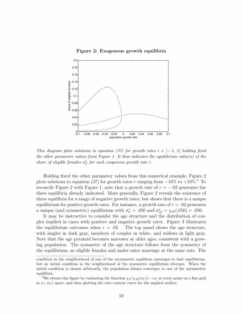
Figure 2: Exogenous growth equilibria
population growth rate
sha
re o
f elig
ible
fe
male
s
−0.1 −0.08 −0.06 −0.04 −0.02 0 0.02 0.04 0.06 0.08 0.10
0.02
0.04
0.06
0.08
0.1
0.12
0.14
0.16
0.18
0.2
This diagram plots solutions to equation (37) for growth rates r ∈ [−.1, .1] holding fixed
the other parameter values from Figure 1. It thus indicates the equilibrium value(s) of the
share of eligible females σ∗F for each exogenous growth rate r.
Holding fixed the other parameter values from this numerical example, Figure 2plots solutions to equation (37) for growth rates r ranging from −10% to +10%.5 Toreconcile Figure 2 with Figure 1, note that a growth rate of r = −.02 generates thethree equilibria already indicated. More generally, Figure 2 reveals the existence ofthree equilibria for a range of negative growth rates, but shows that there is a uniqueequilibrium for positive growth rates. For instance, a growth rate of r = .02 generatesa unique (and symmetric) equilibrium with σ∗F = .050 and σ∗M = χM(.050) = .050.
It may be instructive to consider the age structure and the distribution of cou-ples implied in cases with positive and negative growth rates. Figure 3 illustratesthe equilibrium outcomes when r = .02. The top panel shows the age structure,with singles in dark gray, members of couples in white, and widows in light gray.Note that the age pyramid becomes narrower at older ages, consistent with a grow-ing population. The symmetry of the age structure follows from the symmetry ofthe equilibrium, as eligible females and males enter marriage at the same rate. The
condition in the neighborhood of one of the asymmetric equilibria converges to that equilibrium,but an initial condition in the neighborhood of the symmetric equilibrium diverges. When theinitial condition is chosen arbitrarily, the population always converges to one of the asymmetricequilibria.
5We obtain this figure by evaluating the function χF (χM (σF ))−σF at every point on a fine gridin (r, σF ) space, and then plotting the zero contour curve for the implied surface.
10

Figure 3: Equilibrium population structure given r = .02
Age structure
1.5 1 0.5 0 0.5 1 1.50
10
20
30
40
50
60
70
80
number of males number of females
age
(in y
ears
)
Couples distribution
male age (in years)
fem
ale
age
(in y
ears
)
0 10 20 30 40 50 60 70 800
10
20
30
40
50
60
70
80
These diagrams show the unique equilibrium population structure for r = .02 given the
other parameter values from Figure 1. The top panel depicts the age structure, with singles
in dark gray, members of couples in white, and widows in light gray. The horizontal dotted
lines indicate the range of eligibility for matching. The bottom panel depicts the distribution
of couples, with darker shades of gray indicating higher densities.
11

Figure 4: Equilibrium population structure given r = −.02
Age structure
5 4 3 2 1 0 1 2 3 4 50
10
20
30
40
50
60
70
80
number of males number of females
age (
in y
ea
rs)
Couples distribution
male age (in years)
fem
ale
age
(in y
ears
)
0 10 20 30 40 50 60 70 800
10
20
30
40
50
60
70
80
These diagrams show one of the asymmetric equilibrium population structures for r = −.02
and the other parameter values from Figure 1. The top panel depicts the age structure, with
singles in dark gray, members of couples in white, and widows in light gray. The horizontal
dotted lines indicate the range of eligibility for matching. The bottom panel depicts the
distribution of couples, with darker shades of gray indicating higher densities.
12

bottom panel gives a contour plot of the couples distribution, with darker shadesof gray corresponding to higher densities. While our model presumes that the forceof attraction is constant for all eligible pairs regardless of age, the equilibrium dis-tribution of couples displays strong positive sorting by age. Intuitively, matchingis driven by availability, and most eligible singles are young (as shown by the agedistribution).
Figure 4 illustrates one of the (stable) asymmetric equilibrium outcomes whenr = −.02. Note that the age pyramid becomes wider at older ages, consistent witha shrinking population. Given the asymmetry of this equilibrium (σ∗F = .012 andσ∗M = .112), the relatively large share of eligible males causes eligible females toquickly enter marriage. Conversely, the relatively small share of eligible femalescreates a backlog of eligible males. While the distribution of couples shows somepositive sorting by age, the asymmetry of the age distribution of eligible singlesinduces asymmetry of the couples distribution, with husbands typically older thanwives. Note also that the couples distribution is now skewed toward older couples,reflecting the negative growth rate of the population.
Figures 5 and 6 provide some sense of how the solutions of equation (37) vary withthe parameters of the model. In Figure 5, we fix αF = αM = 20, γF = γM = 60,and ωF = ωM = 80, and then consider µ ∈ {.5, 1, 2, 4} and s ∈ {.95, 1, 1.05}. Foreach combination of parameters, the diagram gives the equilibrium share of eligiblefemales σ∗F for every growth rate r ∈ [−.1, .1]. The diagrams suggest that multipleequilibria arise when the matching rate µ is sufficiently large, and the sex ratio atbirth s is close enough to 1. In Figure 6, we repeat the same exercise, but withγF = γM = 50 and µ ∈ {1, 2, 3, 4}. Comparison of Figures 5 and 6 suggests thatscope for multiple equilibria decreases as the range of eligible ages shrinks. Fixingthe other parameters, additional examples (not reported) indicate that a matchingrate of µ ≥ 5 is needed to induce multiple equilibria when γF = γM = 45, and thata matching rate of µ ≥ 10 is needed when γF = γM = 40.
Perhaps the most interesting observation from Figures 5 and 6 is that multipleequilibria arise only when the growth rate is negative. This result also holds foradditional examples (not reported) covering more of the parameter space and alsopermitting asymmetry between the sexes in the first age of eligibility (α), the last ageof eligibility (γ), and the age at death (ω). In the Appendix, using the continuous-time analogs of equations (33) and (34), we provide a formal proof that non-negativegrowth implies a unique equilibrium. Arguably, because populations with negativegrowth ultimately become extinct, this result might seem to undermine our emphasison the potential for multiple equilibria. But as shown by Figures 5 and 6, multipleequilibria can arise even when the growth rate is only slightly below zero. Further,as we will see in the next section when we endogenize the growth rate, it may bepossible (for a given set of parameter values) to have one equilibrium with a positivegrowth rate and other equilibria with negative growth rates.
13

Figure 5: Equilibrium outcomes given γ = 60
growth rate
elig
ible
fem
ales
µ = 4, s = 0.95
−0.1 0 0.10
0.05
0.1
0.15
0.2
growth rate
elig
ible
fem
ales
µ = 2, s = 0.95
−0.1 0 0.10
0.05
0.1
0.15
0.2
growth rate
elig
ible
fem
ales
µ = 1, s = 0.95
−0.1 0 0.10
0.05
0.1
0.15
0.2
growth rate
elig
ible
fem
ales
µ = 0.5, s = 0.95
−0.1 0 0.10
0.05
0.1
0.15
0.2
growth rate
elig
ible
fem
ales
µ = 4, s = 1
−0.1 0 0.10
0.05
0.1
0.15
0.2
growth rate
elig
ible
fem
ales
µ = 2, s = 1
−0.1 0 0.10
0.05
0.1
0.15
0.2
growth rate
elig
ible
fem
ales
µ = 1, s = 1
−0.1 0 0.10
0.05
0.1
0.15
0.2
growth rate
elig
ible
fem
ales
µ = 0.5, s = 1
−0.1 0 0.10
0.05
0.1
0.15
0.2
growth rate
elig
ible
fem
ales
µ = 4, s = 1.05
−0.1 0 0.10
0.05
0.1
0.15
0.2
growth rate
elig
ible
fem
ales
µ = 2, s = 1.05
−0.1 0 0.10
0.05
0.1
0.15
0.2
growth rate
elig
ible
fem
ales
µ = 1, s = 1.05
−0.1 0 0.10
0.05
0.1
0.15
0.2
growth rate
elig
ible
fem
ales
µ = 0.5, s = 1.05
−0.1 0 0.10
0.05
0.1
0.15
0.2
Following the format of Figure 2, each diagram plots solutions to equation (37), indicating
equilibrium value(s) of the share of eligible females σ∗F for each exogenous growth rate
r ∈ [−.1, .1]. The parameter values αF = αM = 20, γF = γF = 60, ωF = ωM = 80, and
H = 1/h = 10 are fixed across all diagrams. The matching rate µ and the sex ratio at birth
s vary across diagrams as indicated.
14

Figure 6: Equilibrium outcomes given γ = 50
growth rate
elig
ible
fem
ales
µ = 4, s = 0.95
−0.1 0 0.10
0.05
0.1
0.15
0.2
growth rate
elig
ible
fem
ales
µ = 3, s = 0.95
−0.1 0 0.10
0.05
0.1
0.15
0.2
growth rate
elig
ible
fem
ales
µ = 2, s = 0.95
−0.1 0 0.10
0.05
0.1
0.15
0.2
growth rate
elig
ible
fem
ales
µ = 1, s = 0.95
−0.1 0 0.10
0.05
0.1
0.15
0.2
growth rate
elig
ible
fem
ales
µ = 4, s = 1
−0.1 0 0.10
0.05
0.1
0.15
0.2
growth rate
elig
ible
fem
ales
µ = 3, s = 1
−0.1 0 0.10
0.05
0.1
0.15
0.2
growth rate
elig
ible
fem
ales
µ = 2, s = 1
−0.1 0 0.10
0.05
0.1
0.15
0.2
growth rate
elig
ible
fem
ales
µ = 1, s = 1
−0.1 0 0.10
0.05
0.1
0.15
0.2
growth rate
elig
ible
fem
ales
µ = 4, s = 1.05
−0.1 0 0.10
0.05
0.1
0.15
0.2
growth rate
elig
ible
fem
ales
µ = 3, s = 1.05
−0.1 0 0.10
0.05
0.1
0.15
0.2
growth rate
elig
ible
fem
ales
µ = 2, s = 1.05
−0.1 0 0.10
0.05
0.1
0.15
0.2
growth rate
elig
ible
fem
ales
µ = 1, s = 1.05
−0.1 0 0.10
0.05
0.1
0.15
0.2
Following the format of Figure 2, each diagram plots solutions to equation (37), indicating
equilibrium value(s) of the share of eligible females σ∗F for each exogenous growth rate
r ∈ [−.1, .1]. The parameter values αF = αM = 20, γF = γF = 50, ωF = ωM = 80, and
H = 1/h = 10 are fixed across all diagrams. The matching rate µ and the sex ratio at birth
s vary across diagrams as indicated.
15
4 Endogenous growth
We now consider the model with endogenous growth, replacing equations (24-25)with equations (10-11), so that population dynamics are given by equations (5-13).
In the absence of early mortality (equations 22-23), equation (7) becomes
C(i+ 1, j + 1, t+ 1) = C(i, j, t) + Φ(i, j, t) (39)
Given the recursive structure of this equation, and the age ranges over which indi-viduals may form couples (equation 15), we obtain
C(i, j, t) =
τ(i,j)∑τ=τ(i,j)
Φ(i− τ, j − τ, t− τ) (40)
where
τ(i, j) = max{i− γFH + 1, j − γMH + 1, 1} (41)
τ(i, j) = min{i− αFH, j − αMH} (42)
Intuitively, τ(i, j) is the number of periods since an ij couple could have most recentlyformed, and τ(i, j) is the number of periods since an ij couple could have firstformed. Note that τ(i, j) = 1 if both the female and male are currently eligible formatching. If either the female or the male is not yet eligible, then τ(i, j) < 0 andhence C(i, j, t) = 0.
We continue to consider equilibria with persistent distributions. Equation (40)may thus be written as
C(i, j) =
τ(i,j)∑τ=τ(i,j)
Φ(i− τ, j − τ) (1 + hr)−τ (43)
where the time index t has been suppressed. Given our specification of the matchingfunction (equations 3 and 14), and using equations (30-32) to determine F (i) andM(j), we obtain
C(i, j) =shµ
N
τ(i,j)∑τ=τ(i,j)
(1 + hr)−i−j+τ (1− hµσM)i−τ−αFH(1− hµσF )j−τ−αMH (44)
where population size N is given by equation (35). Fixing the parameters of themodel, each element of the couples distribution is thus determined by the growthrate r, the share of eligible females σF , and the share of eligible males σM .
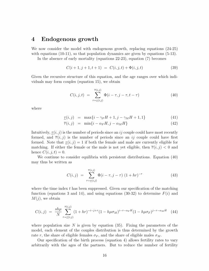
Our specification of the birth process (equation 4) allows fertility rates to varyarbitrarily with the ages of the partners. But to reduce the number of fertility
16
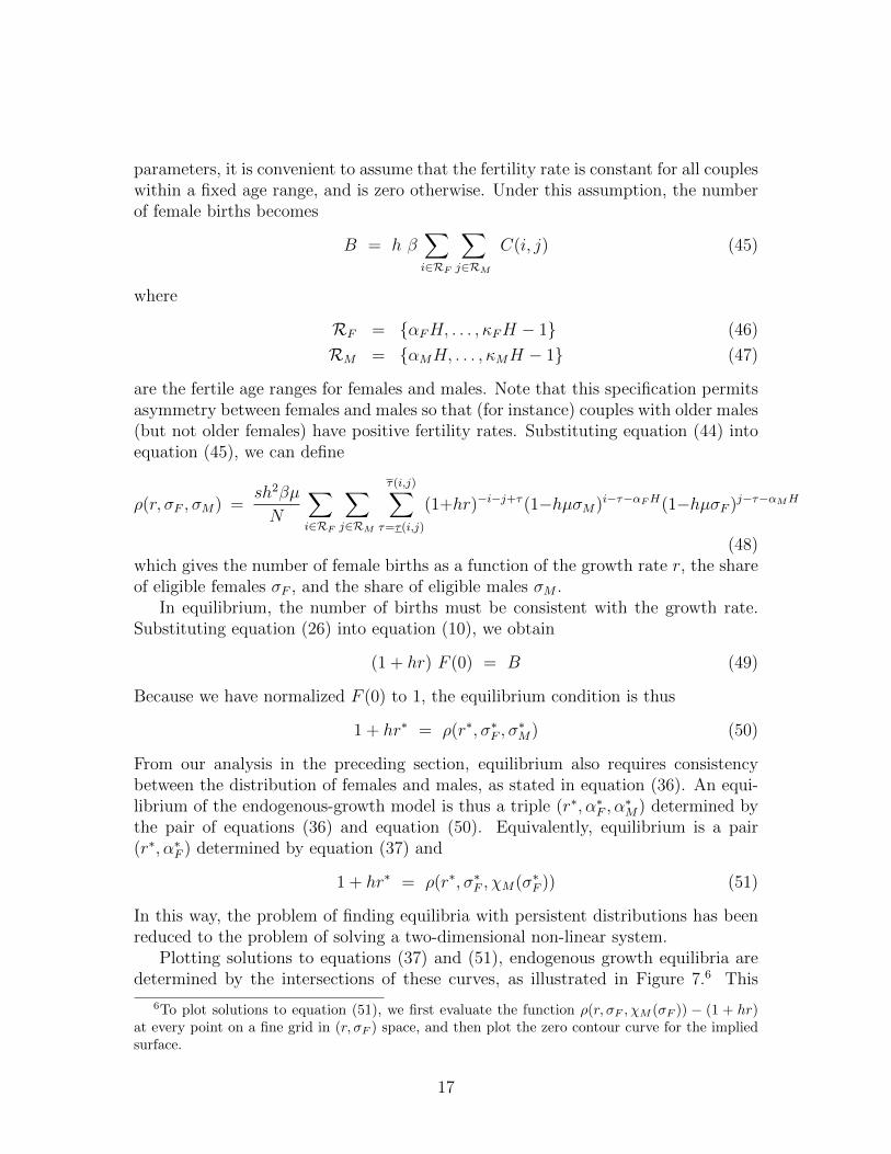
parameters, it is convenient to assume that the fertility rate is constant for all coupleswithin a fixed age range, and is zero otherwise. Under this assumption, the numberof female births becomes
B = h β∑i∈RF
∑j∈RM
C(i, j) (45)
where
RF = {αFH, . . . , κFH − 1} (46)
RM = {αMH, . . . , κMH − 1} (47)
are the fertile age ranges for females and males. Note that this specification permitsasymmetry between females and males so that (for instance) couples with older males(but not older females) have positive fertility rates. Substituting equation (44) intoequation (45), we can define
ρ(r, σF , σM) =sh2βµ
N
∑i∈RF
∑j∈RM
τ(i,j)∑τ=τ(i,j)
(1+hr)−i−j+τ (1−hµσM)i−τ−αFH(1−hµσF )j−τ−αMH
(48)which gives the number of female births as a function of the growth rate r, the shareof eligible females σF , and the share of eligible males σM .
In equilibrium, the number of births must be consistent with the growth rate.Substituting equation (26) into equation (10), we obtain
(1 + hr) F (0) = B (49)
Because we have normalized F (0) to 1, the equilibrium condition is thus
1 + hr∗ = ρ(r∗, σ∗F , σ∗M) (50)
From our analysis in the preceding section, equilibrium also requires consistencybetween the distribution of females and males, as stated in equation (36). An equi-librium of the endogenous-growth model is thus a triple (r∗, α∗F , α
∗M) determined by
the pair of equations (36) and equation (50). Equivalently, equilibrium is a pair(r∗, α∗F ) determined by equation (37) and
1 + hr∗ = ρ(r∗, σ∗F , χM(σ∗F )) (51)
In this way, the problem of finding equilibria with persistent distributions has beenreduced to the problem of solving a two-dimensional non-linear system.
Plotting solutions to equations (37) and (51), endogenous growth equilibria aredetermined by the intersections of these curves, as illustrated in Figure 7.6 This
6To plot solutions to equation (51), we first evaluate the function ρ(r, σF , χM (σF )) − (1 + hr)at every point on a fine grid in (r, σF ) space, and then plot the zero contour curve for the impliedsurface.
17
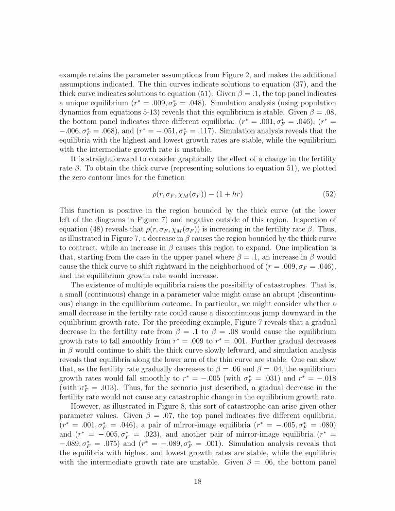
example retains the parameter assumptions from Figure 2, and makes the additionalassumptions indicated. The thin curves indicate solutions to equation (37), and thethick curve indicates solutions to equation (51). Given β = .1, the top panel indicatesa unique equilibrium (r∗ = .009, σ∗F = .048). Simulation analysis (using populationdynamics from equations 5-13) reveals that this equilibrium is stable. Given β = .08,the bottom panel indicates three different equilibria: (r∗ = .001, σ∗F = .046), (r∗ =−.006, σ∗F = .068), and (r∗ = −.051, σ∗F = .117). Simulation analysis reveals that theequilibria with the highest and lowest growth rates are stable, while the equilibriumwith the intermediate growth rate is unstable.
It is straightforward to consider graphically the effect of a change in the fertilityrate β. To obtain the thick curve (representing solutions to equation 51), we plottedthe zero contour lines for the function
ρ(r, σF , χM(σF ))− (1 + hr) (52)
This function is positive in the region bounded by the thick curve (at the lowerleft of the diagrams in Figure 7) and negative outside of this region. Inspection ofequation (48) reveals that ρ(r, σF , χM(σF )) is increasing in the fertility rate β. Thus,as illustrated in Figure 7, a decrease in β causes the region bounded by the thick curveto contract, while an increase in β causes this region to expand. One implication isthat, starting from the case in the upper panel where β = .1, an increase in β wouldcause the thick curve to shift rightward in the neighborhood of (r = .009, σF = .046),and the equilibrium growth rate would increase.
The existence of multiple equilibria raises the possibility of catastrophes. That is,a small (continuous) change in a parameter value might cause an abrupt (discontinu-ous) change in the equilibrium outcome. In particular, we might consider whether asmall decrease in the fertilty rate could cause a discontinuous jump downward in theequilibrium growth rate. For the preceding example, Figure 7 reveals that a gradualdecrease in the fertility rate from β = .1 to β = .08 would cause the equilibriumgrowth rate to fall smoothly from r∗ = .009 to r∗ = .001. Further gradual decreasesin β would continue to shift the thick curve slowly leftward, and simulation analysisreveals that equilibria along the lower arm of the thin curve are stable. One can showthat, as the fertility rate gradually decreases to β = .06 and β = .04, the equilibriumgrowth rates would fall smoothly to r∗ = −.005 (with σ∗F = .031) and r∗ = −.018(with σ∗F = .013). Thus, for the scenario just described, a gradual decrease in thefertility rate would not cause any catastrophic change in the equilibrium growth rate.
However, as illustrated in Figure 8, this sort of catastrophe can arise given otherparameter values. Given β = .07, the top panel indicates five different equilibria:(r∗ = .001, σ∗F = .046), a pair of mirror-image equilibria (r∗ = −.005, σ∗F = .080)and (r∗ = −.005, σ∗F = .023), and another pair of mirror-image equilibria (r∗ =−.089, σ∗F = .075) and (r∗ = −.089, σ∗F = .001). Simulation analysis reveals thatthe equilibria with highest and lowest growth rates are stable, while the equilibriawith the intermediate growth rate are unstable. Given β = .06, the bottom panel
18

Figure 7: Endogenous growth equilibria
β = .1
−0.1 −0.08 −0.06 −0.04 −0.02 0 0.02 0.04 0.06 0.08 0.10
0.02
0.04
0.06
0.08
0.1
0.12
0.14
0.16
0.18
0.2
population growth rate
sh
are
of e
ligib
le f
em
ale
s
β = .08
−0.1 −0.08 −0.06 −0.04 −0.02 0 0.02 0.04 0.06 0.08 0.10
0.02
0.04
0.06
0.08
0.1
0.12
0.14
0.16
0.18
0.2
population growth rate
share
of elig
ible
fem
ale
s
These diagrams assume µ = 3, s = 1, αF = αM = 20, γF = γM = 60, ωF = ωM = 80,
H = 1/h = 10, κF = 40, and κM = 60. The fertility rate β varies across diagrams as
indicated. The thin curves indicate solutions to equation (37); the thick curves indicate
solutions to equation (51). Equilibria (r∗, σ∗F ) correspond to the intersections of these
curves.
19

Figure 8: A catastrophe
β = .07
−0.14 −0.12 −0.1 −0.08 −0.06 −0.04 −0.02 0 0.02 0.040
0.02
0.04
0.06
0.08
0.1
0.12
0.14
0.16
0.18
0.2
population growth rate
shar
e of
elig
ible
fem
ales
β = .06
−0.14 −0.12 −0.1 −0.08 −0.06 −0.04 −0.02 0 0.02 0.040
0.02
0.04
0.06
0.08
0.1
0.12
0.14
0.16
0.18
0.2
population growth rate
shar
e of
elig
ible
fem
ales
These diagrams assume µ = 3, s = 1, αF = αM = 15, γF = γM = 60, ωF = ωM = 80,
H = 1/h = 10, and κF = κM = 40. The fertility rate β varies across diagrams as indicated.
The thin curves indicate solutions to equation (37); the thick curves indicate solutions to
equation (51). Equilibria (r∗, σ∗F ) correspond to the intersections of these curves.
20

indicates three different equilibria: (r∗ = −.006, σ∗F = .043), and a pair of mirror-image equilibria (r∗ = −.109, σ∗F = .051) and (r∗ = −.109, σ∗F = .001). Simulationanalysis reveals that the equilibrium with the higher growth rate is unstable, whilethe equilibria with lower growth rates are stable.
The instability of the equilibrium with r∗ = −.006 for β = .06 creates the po-tential for a catastrophe. Suppose the fertility rate is β = .07 and the populationis initially in the positive growth equilibrium. If the fertility rate decreases slightlyto β = .06, the population moves from (r = .001, σF = .046) toward the equilibrium(r∗ = −.006, σ∗F = .043). However, because this equilibrium is not stable, the pop-ulation will diverge (slowly at first) from this outcome. In the process, the growthrate will continue to fall until the population ultimately reaches one of the stableequilibria. Thus, given a small change in the fertility rate from from .07 to .06, theequilibrium growth rate jumps discontinously downward from 0% to nearly −11%.
Equations (37) and (51) determine existence but not stability of equilibria, and itis important to recognize the high dimensionality of the dynamical system composedof equations (5-13). Nevertheless, a naive interpretation of Figures 7 and 8 as phasediagrams for a two-dimensional dynamical system does provide some insight intodisequilibrium dynamics. On this interpretation,
sign{dσF/dt} = sign{χF (χM(σF ))− σF} (53)
sign{dr/dt} = sign{ρ(r, σF , χM(σF ))− (1 + hr)} (54)
To illustrate, consider again Figure 8. For the top panel (β = .07), these dynamicssuggest stability of the equilibrium (r∗ = .001, σ∗F = .046). Within the neighborhoodof this equilibrium, both r and σF would converge to the equilibrium levels. Incontrast, for the bottom panel (β = .06), these dynamics suggest instability of theequilibrium (r∗ = −.006, σ∗F = .043). Within the neighborhood of this equilibrium, rwould converge to the equilibrium, but σF would diverge. Consistent with this naivephase-diagram analysis, simulations reveal that the population initially diverges byfollowing a path along the thick black curve away from the unstable equilibrium.
However, these “phase diagrams” may be a poor guide to disequilibrium dynamicsin other cases, especially given the potential for limit cycles.7 Figure 9 illustrates.In the top panel, χF (χM(σF )) − σF is negative above the thin curve and positivebelow it, while ρ(r, σF , χM(σF )) − (1 + hr) is positive to the left of the thick curveand negative to the left. Equations (53-54) would thus suggest convergence of thepopulation to the equilibrium (r∗ = .028, σ∗F = .106). But simulation analysis revealsthe population actually converges to the limit cycle indicated by the dotted curve inthe top panel and the time paths in the bottom panel.
Further examples suggest that limit cycles arise only when the reproductive ageranges are relatively short. That is, fixing the earliest ages at which individualsreproduce (αF and αM), limit cycles arise only when the final ages (κF and κM) are
7See Caswell and Weeks (1986) for a discussion of limit cycles in two-sex models.
21
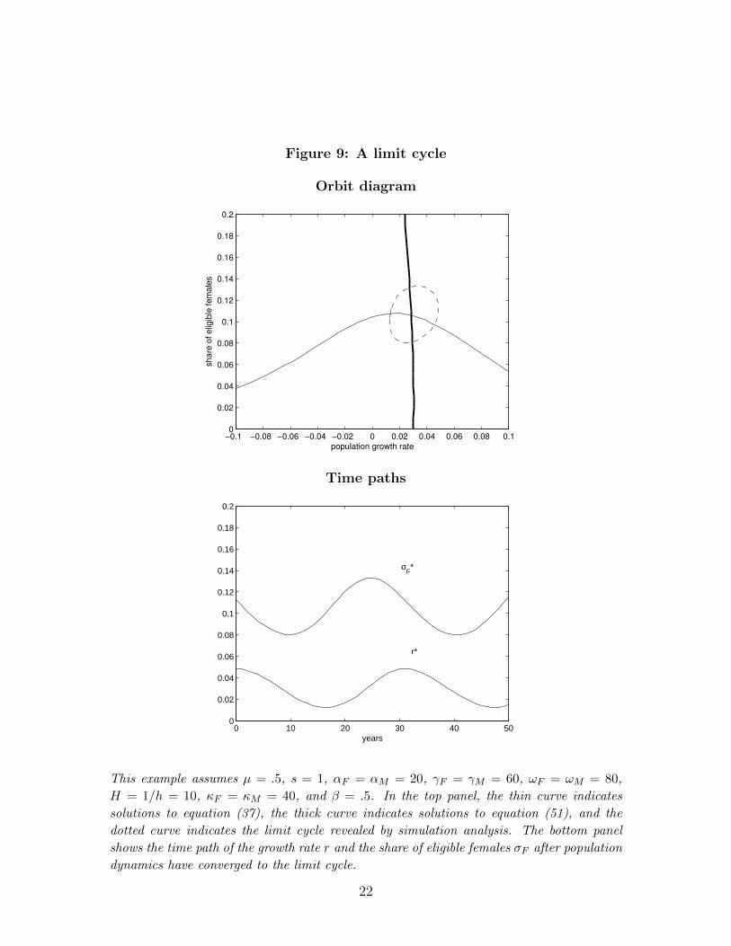
Figure 9: A limit cycle
Orbit diagram
−0.1 −0.08 −0.06 −0.04 −0.02 0 0.02 0.04 0.06 0.08 0.10
0.02
0.04
0.06
0.08
0.1
0.12
0.14
0.16
0.18
0.2
population growth rate
sh
are
of e
ligib
le fe
ma
les
Time paths
0 10 20 30 40 500
0.02
0.04
0.06
0.08
0.1
0.12
0.14
0.16
0.18
0.2
years
r*
σF*
This example assumes µ = .5, s = 1, αF = αM = 20, γF = γM = 60, ωF = ωM = 80,
H = 1/h = 10, κF = κM = 40, and β = .5. In the top panel, the thin curve indicates
solutions to equation (37), the thick curve indicates solutions to equation (51), and the
dotted curve indicates the limit cycle revealed by simulation analysis. The bottom panel
shows the time path of the growth rate r and the share of eligible females σF after population
dynamics have converged to the limit cycle.
22
relatively low. To illustrate, Figure 10 varies these parameters while holding fixedthe other parameters from Figure 9. The dotted curves on the upper-left diagramsindicate that the population converges to a limit cycles, while the absence of dottedcurves in the other diagrams indicates that the population converges to the steadystate determined by the intersection of the thin and thick curves.
5 Conclusion
This paper examines an age-structured two-sex model in which couples dissolve onlythrough the death of a spouse, and widows never remarry. Additional simplifyingassumptions on the matching function (individuals meet through random mixing ofthe population; eligible singles have no age preference over potential partners) yielda highly tractable model. In the exogenous-growth version, an equilibrium is fullycharacterized by a single variable (the share of eligible females in the population). Inthe endogenous-growth version, an equilibrium is characterized by a pair of variables(the growth rate as well as the share of eligible females). In both versions, equilibriacan be determined through simple graphical methods.
While other age-structured two-sex models are more general and more realistic,their complexity has precluded analysis of the stability and uniqueness of equilibria.In contrast, the tractability of the present model permits some new insight intoconditions under which multiple equilibria arise. In the exogenous-growth model, weprove that multiple equilibria arise only if the growth rate is negative. Numericalexamples further indicate that multiplicity requires either a high matching rate ora large range of eligible ages. In the endogenous-growth model, numerical examplesdemonstrate the potential for multiple equilibria, catastrophes, and limit cycles.
Though the practical importance of these results is somewhat difficult to judgewithout generalization of the model and calibration of model parameters, our findingsmight suggest that multiple equilibria are not likely to arise in realistic settingsgiven the ranges of parameter values that would be associated with observed humanpopulations. In particular, while our leading examples (Figures 1 to 4) assumeda very large range of eligible ages (20 to 60 years), we might expect this range tobe smaller in observed populations (at least under the maintained assumption thateligible singles are indifferent to the age of potential partners). Further, intuitionsuggests that divorce and remarriage, by increasing the availability of eligible singlesat older ages, might further limit the potential for multiple equilibria.
On the other hand, we note that the exogenous-growth version of our model issimilar to the MSQUEEZ model developed by Schoen (1983). In parallel to our anal-ysis, Schoen derived the equilibrium population structure for exogenous growth ratesbetween −20% and +20%. But in contrast to our analysis, the iterative procedurehe used to compute these equilibria would not have detected the existence of multi-
23

Figure 10: Equilibrium outcomes by κM and κF
−0.1 0 0.10
0.1
0.2
growth rate
elig
ible
fem
ales
κM
= 35, κF = 35
−0.1 0 0.10
0.1
0.2
growth rate
elig
ible
fem
ales
κM
= 40, κF = 35
−0.1 0 0.10
0.1
0.2
growth rate
elig
ible
fem
ales
κM
= 45, κF = 35
−0.1 0 0.10
0.1
0.2
growth rate
elig
ible
fem
ales
κM
= 50, κF = 35
−0.1 0 0.10
0.1
0.2
growth rate
elig
ible
fem
ales
κM
= 35, κF = 40
−0.1 0 0.10
0.1
0.2
growth rate
elig
ible
fem
ales
κM
= 40, κF = 40
−0.1 0 0.10
0.1
0.2
growth rate
elig
ible
fem
ales
κM
= 45, κF = 40
−0.1 0 0.10
0.1
0.2
growth rate
elig
ible
fem
ales
κM
= 50, κF = 40
−0.1 0 0.10
0.1
0.2
growth rate
elig
ible
fem
ales
κM
= 35, κF = 45
−0.1 0 0.10
0.1
0.2
growth rateel
igib
le fe
mal
es
κM
= 40, κF = 45
−0.1 0 0.10
0.1
0.2
growth rate
elig
ible
fem
ales
κM
= 45, κF = 45
−0.1 0 0.10
0.1
0.2
growth rate
elig
ible
fem
ales
κM
= 50, κF = 45
The parameter values µ = .5, s = 1, αF = αM = 20, γF = γM = 60, ωF = ωM = 80,
H = 1/h = 5, and β = .5 are fixed across all diagrams. The parameters κF and κM vary
across the diagrams as indicated. Following the format of the top panel of Figure 9, the
dotted lines indicate limit cycles revealed by simulation analysis. For the diagrams without
dotted lines, the population converges to the steady steady indicated by the intersection of
the thin and thick curves.
24
ple equilibria.8 Perhaps there was no potential for multiple equilibria given Schoen’s(harmonic mean) specification of the matching function or his (empirically grounded)specification of matching parameters. But our present results might encourage futureresearchers to consider this possibility.
Our finding that multiple equilibria arise in the exogenous-growth model onlyif the growth rate is negative might seem to further limit the practical relevanceof our results. Obviously, populations with negative growth rates will ultimatelybecome extinct. However, our examples indicate that multiple equilibria can ariseeven when the growth rate is only slightly negative. While speculative, our findingsmight encourage researchers to explore the theoretical potential for multiple equilib-ria or even catastrophic change in countries currently experiencing negative growthor below-replacement fertility.
The tractability of the present model allows equilibria to be determined througha two-equation system that can be analyzed graphically. Future theoretical workmight see how far the model can be generalized without losing this attractive impli-cation. While tractability hinges on the two simplifying assumptions on the matchingfunction, other simplifying assumptions were made merely for convenience. In par-ticular, it would be straightforward to allow arbitrary patterns of mortality (δF andδM varying by the individual’s age) or fertility (β varying by the ages of partners).Potentially, the model could also be extended to allow divorce and remarriage with-out moving beyond our two-equation framework, since the distribution of coupleswould still be determined by the distributions of singles, though the form of thedependence would become more complicated.
While motivated by tractability considerations, our key assumptions on the match-ing function might be defended on substantive grounds. In the absence of consensuson the best specification of the matching function (Pollard 1997, Ianelli et al 2005),random mixing provides a useful baseline. Age preference among eligible singles maybe weaker than generally assumed (Bhrolchain 2001), and we have shown that strongpositive sorting by age can arise solely through availability considerations (recall thelower panel of Figure 2). Nevertheless, empirical realism surely warrants more gen-eral specifications of the matching function. We hope that the present paper, bybeginning to identify the conditions under which multiple equilibria arise, will proveuseful as researchers continue to grapple with more general (and harder to analyze)age-structured two-sex models.
8In that procedure, initial conditions were taken from empirical one-sex life tables. A widerrange of initial conditions would be needed to address the existence (or non-existence) of multipleequilibria.
25
6 Appendix
In this appendix, we prove that multiple equilibria arise in the exogeneous-growthmodel only if the growth rate is negative.
The continuous-time analogs of equations (33) and (34) are
χF (σM) =1
Ne−αF r
γF−αF∫0
e−(r+µσM )i di (55)
χM(σF ) =1
Ns e−αMr
γM−αM∫0
e−(r+µσF )j dj (56)
and hence the derivatives are
χF′(σM) = −µ 1
Ne−αF r
γF−αF∫0
i e−(r+µσM )i di (57)
χM′(σF ) = −µ 1
Ns e−αMr
γM−αM∫0
j e−(r+µσF )j dj (58)
The slope of the compound function χF (χM(σF )) can be written
χF′(χM(σF )) · χM ′(σF ) (59)
which, evaluated at the fixed point σ∗F , becomes
χF′(σ∗M) · χM ′(σ∗F ) (60)
Using equation (36), this product may be rewritten as
σ∗M χF′(σ∗M)
χF (σ∗M)· σ∗F χM
′(σ∗F )
χM(σ∗F )(61)
which is equal to
σ∗M µγF−αF∫
0
i e−(r+µσ∗M )i di
γF−αF∫0
e−(r+µσ∗M )i di
·σ∗F µ
γM−αM∫0
j e−(r+µσ∗F )j dj
γM−αM∫0
e−(r+µσ∗F )j dj
(62)
Note that both terms in equation (62) take the form
ζ(r) =x∫ b0i e−(r+x)i di∫ b
0e−(r+x)i di
(63)
26

where ζ(0) < 1 for b < ∞, and ζ ′(r) < 0. Thus, when the growth rate r is non-negative, both terms in equation (62) are less than 1. Consequently, the slope of thecompound function χF (χM(σF )) must be less than 1 at any fixed point σ∗F . Recallingthat the compound function is continuous and increasing and satisfies equation (38),this guarantees the existence of a unique fixed point.
References
Allman, Elizabeth S. and John A. Rhodes (2004) Mathematical Models in Biology:An Introduction. New York: Cambridge University Press.
Bhrolchain, Maire Ni (2001) “Flexibility in the Marriage Market,” Population: AnEnglish Selection 13:9-47.
Caswell, H and D E Weeks (1986) “Two-Sex Models: Chaos, Extinction, and OtherDynamic Consequences of Sex,” American Naturalist 128:707-735.
Guilmoto, Christophe Z (2012) “Skewed Sex Ratios at Birth and Future MarriageSqueeze in China and India, 2005-2100,” Demography 49:77-100.
Hadeler, K P (1989) “Pair Formation in Age-Structured Populations,” Acta Appli-candae Mathematicae 14:91-102.
—— (1993) “Pair Formation Models with Maturation Period,” Journal of Mathe-matical Biology 32:1-15.
Hoppensteadt, Frank (1975) Mathematical Theories of Populations: Demographics,Genetics and Epidemics. Philadelphia: SIAM.
Iannelli, M, M Martcheva, and F A Milner (2005) Gender-Structured PopulationModeling: Mathematical Methods, Numerics, and Simulations. Philadelphia:SIAM.
Inaba, Hisashi (1993) “An Age-Structured Two-Sex Model for Human PopulationReproduction by First Marriage,” Working Paper Series No. 15, Institute ofPopulation Problems, Ministry of Health and Welfare, Japan.
—— (2000) “Persistent Age Distributions for an Age-Structured Two-Sex PopulationModel,” Mathematical Population Studies 7:365-398.
Keyfitz, Nathan (1972) “The Mathematics of Sex and Marriage” in Proceedings ofthe Sixth Berkeley Symposium on Mathematical Statistics and Probability, Vol4. Berkeley: University of California Press.
Martcheva, Maia (1999) “Exponential Growth in Age-Structured Two-Sex Popula-tions,” Mathematical Biosciences 157:1-22.
27

Pollak, Robert A (1986) “A Reformulation of the Two-Sex Problem,” Demography23:247-259.
—— (1990) “Two-Sex Demographic Models,” Journal of Political Economy 98:399-420.
Pollard, J H (1997) “Modelling the Interaction Between the Sexes,” Mathematicaland Computational Modeling 26:11-24.
Pruss, Jan and Wilhelm Schappacher (1993) “Persistent Age Distributions for aPair-Formation Model,” Journal of Mathematical Biology 33:17-33.
Schoen, Robert (1983) “Measuring the Tightness of a Marriage Squeeze,” Demogra-phy 20:61-78.
—— (1988) Modeling Multigroup Populations. New York: Plenum Press.
28