multiphysics simulation of corona discharge induced … · multiphysics simulation of corona...

Multiphysics simulation of corona discharge

induced ionic wind

Davide Cagnoni∗1,2, Francesco Agostini2, Thomas Christen2, Carlode Falco1,3, Nicola Parolini1 and Ivica Stevanovic2,4

1MOX - Dipartimento di Matematica “F. Brioschi,” Politecnico di Milano, 20133Milano, Italy

2ABB Switzerland Ltd., Corporate Research, CH-5405 Baden-Dattwil, Switzerland3CEN - Centro Europeo di Nanomedicina, 20133 Milano, Italy

4Laboratory of Electromagnetics and Acoustics, Ecole Polytechnique Federale deLausanne, CH-1015 Lausanne, Switzerland

Friday 28th June, 2013

Abstract

Ionic wind devices or electrostatic fluid accelerators are becoming ofincreasing interest as tools for thermal management, in particular for semi-conductor devices. In this work, we present a numerical model for predict-ing the performance of such devices, whose main benefit is the ability toaccurately predict the amount of charge injected at the corona electrode.Our multiphysics numerical model consists of a highly nonlinear stronglycoupled set of PDEs including the Navier-Stokes equations for fluid flow,Poisson’s equation for electrostatic potential, charge continuity and heattransfer equations. To solve this system we employ a staggered solutionalgorithm that generalizes Gummel’s algorithm for charge transport insemiconductors. Predictions of our simulations are validated by compar-ison with experimental measurements and are shown to closely match.Finally, our simulation tool is used to estimate the effectiveness of thedesign of an electrohydrodynamic cooling apparatus for power electronicsapplications.

PACS: 52.80.-s , 47.65.-dKeywords: corona discharge, electrohydrodynamics, ionic wind, math-

ematical models, numerical approximation, functional iteration

1 Introduction and motivation

Cooling of electric and electronic devices is a continuous challenge for researchersand engineers. Power electronics trends indicate a continuous increase of power

∗Corresponding author: [email protected]

1

arX

iv:1

306.

6578

v1 [

phys

ics.

com

p-ph

] 2

7 Ju

n 20

13

2 Multiphysics simulation of corona discharge induced ionic wind

densities and a shrink of component dimensions. These conditions make thethermal management a pillar to guarantee a safe, reliable and affordable op-eration of electronic components where suitable cooling schemes must be ap-plied. Forced convection air cooling is probably the oldest and still one of themost used approaches for electronic systems cooling. Usually, forced convectionis driven by a fan but, for some applications as, for example, the cooling ofhot spots or enclosure-contained devices, alternative methods based on Electro-Hydrodynamic (EHD) forces have been recently studied and exploited. A repre-sentative example of such methods is that of ionic wind induced by a so calledcorona discharge.

Figure 1 schematically illustrates the phenomenon of corona discharge oc-curring between two electrodes in air. The gas ions formed in the dischargeare accelerated by the electric field and exchange momentum with neutral fluidmolecules, initiating a drag of the bulk fluid which is referred to as ionic wind.The choice of a positive corona is favorable in industrial applications as it leadsto significantly reduced ozone production, and increased durability of the metalelectrodes in comparison to negative corona devices.[1] Therefore, in this study,we focus on the case of DC positive corona wind, where the applied voltageat the electrodes is stationary, gas ionization occurs at the anode and chargecarriers are mainly O+

2 ions, as described in Fig. 1(a).Both experimental and numerical studies of EHD phenomena have been pre-

sented in recent literature. For example, Adamiak and others [2, 3, 4, 5] studiedthe DC and pulsed corona discharge between a needle and a plate collector, usingdifferent numerical methods (FEM, BEM, FCT etc.) for the approximation ofeach equation in the PDE system; Ahmedou and Havet [6, 7, 8] used a commer-cial FEM software to investigate the effect of EHD on turbulent flows; Moreauand Touchard,[9] Huang and others,[10] and Kim and others[11] experimentallystudied different EHD devices designed for cooling or air pumping purpose;Chang, Tsubone and others [12, 13, 14] made extensive experimental study ofthe forced airflow and the corona discharge in a converging duct; Jewell-Larsenand others [15, 16, 17, 18, 19, 20, 21] and Go and others [22, 23, 24, 25, 26]conducted both experimental and numerical studies aimed at designing and ap-plying ionic wind cooling devices to thermal management of electronic devices.

In this paper, we use a numerical approach based on a multiphysics math-ematical model that accounts for all relevant electrostatic, fluid, and thermalaspects of the phenomena being considered. Particular attention is devoted tocorrectly modeling the relation between the electric field at the anode and theamount of charge injected from the anode corona into the neutral gas region.The accuracy of such relation is crucial for increasing the predictive capabil-ity of numerical simulations. Here, we present a novel approach for modelingcharge injection, which is based on enforcing Kaptsov’s hypothesis[27] and isshown to provide good simulation accuracy using few free model parameters.Our approach to the charge injection modeling is compared to those existing inthe literature on a set of benchmark device geometries for which experimentaldata are available.

Cagnoni, Agostini, Christen, de Falco, Parolini, Stevanovic June 2013


Anode

Cathode

IonizationRegion

X+

X

X+

XCollisions

Ionic

Wind

(a) Overall scheme of positive corona in-duced ionic wind.

e-

e-X+

X

Xnew collisions

ionizing collision

high energy electron

cation injection

(b) Zoom on the ionization region to showavalanche charge multiplication.

Figure 1: Schematic representation of positive wire-to-plane corona discharge-induced ionic wind. In ambient air, X represents primarily O2 or N2 molecules,and the dominant ionization reactions are of the type e− + X 2e− + X+.[28]

2 Governing equations

Modeling of EHD systems requires accounting for a number of interplayingphenomena of different physical nature. Figure 2 summarizes such phenomenaand their interactions: electric current due to drifting ions generates bulk fluidflow which, in turn, contributes to ion drift; thermal energy is transported bythe flowing fluid while, at the same time, temperature gradients give rise tobuoyancy forces; finally electric conduction properties of the gas are influencedby temperature, while electric currents act as heat sources via Joule effect.

The system of partial differential equations governing the behavior of eachsubsystem is introduced below together with most of the constitutive relationsfor the system coefficients. The PDEs described below are set in an openbounded domain Ω whose typical geometry is shown in Fig. 3; the domainΩ represents the region in space occupied by bulk neutral fluid and drifting pos-itive ions. In our model, the thickness of the ionization layer around the anode isconsidered to be negligible with respect to the length scale of the overall system.Such region is therefore represented as a portion of the boundary, denoted asΓA in Fig. 3, and the process of ion injection is modeled by enforcing a suitableset of boundary conditions on ΓA. Existing and new models for such boundaryconditions are discussed in Section 3.

Unipolar (positive) electrical discharge in fluid is described by Poisson’sequation

∇ · (ε ~E) = −∇ · (ε∇φ) = qNp, (1a)

coupled with current continuity equation

∂qNp

∂t+∇ ·~j = 0, (1b)



ElectricSubsystem

Fluid FlowSubsystem

ThermalSubsystem

Coulom

bFor

ce

Conve

ction

Convection

Buoyancy

Gas Properties

Joule Effect

Figure 2: Relations between the variables in the EHD system, with arrowspointing to an influenced subsystems from the influencing one. Thicker arrowsindicate stronger interactions, while thinner ones indicate minor influence. Thechart is adapted from Ref. [29].

ΓoutΓin

ΓIΓA

ΓC

Ω

Figure 3: Example domain where all the five possible kinds of boundary aredepicted.

where ε is the electrical permittivity, ~E the electric field, φ the electric potential,q the elementary (proton) charge, Np the number density of (positive) ions. The

current density ~j is given by the sum of three contributions: drift due to electricfield, advection, and diffusion:

~j = qNp

(µ~E + ~v

)− qD∇Np, (2)

µ being the ion mobility in the fluid and ~v the fluid velocity field. The diffusionrate D is related to mobility and temperature T through Einstein’s relation

D = µkBTq−1, (3)

where kB is Boltzmann’s constant. The flow of incompressible Newtonian fluidsis described by the Navier-Stokes equations, which represent the conservationof momentum and mass density:

∂~v

∂t+ (~v · ∇)~v = ν∆~v −∇p+

~fEHD + ~fB

ρ,

∇ · ~v = 0,

(1c)

where ν is the kinematic viscosity, p is the modified (non-hydrostatic) pressurepρ−1 − ~g · ~x, ρ being the gas mass density and ~g the gravity acceleration. The



volume force term on the right hand side of the first equation of (1c) consists

of the sum of electrohydrodynamic force ~fEHD and buoyancy force ~fB. As weconsider single-phase flows with limited temperature gradients, ~fEHD can beexpressed as:[30, 31, 32]

~fEHD = qNp~E. (4)

For buoyancy force, due again to the limited temperature gradients, the Boussi-nesq approximation can be adopted:

~fB = ~g[ρ(T )− ρ] = ~g [ρβexp(Tref)(T − Tref)] , (5)

where βexp is the thermal expansion coefficient, and the dependence of the gasdensity ρ(T ) on temperature T is linearized around a certain reference temper-ature Tref , at which the reference density ρ is taken. Finally, the temperatureequation, which describes heat transfer, reads

∂T

∂t+ ~v · ∇T − k

ρCV∆T =

Q

ρCV, (1d)

where k is the heat conductivity and CV the mass specific heat. The thermalpower production Q on the right hand side of (1d) can be expressed as a balanceof terms accounting for the Joule heating caused by the current density ~j andthe mechanical power provided by the EHD force ~fEHD:

Q = ~j · ~E − ~v · ~fEHD = (qNpµ~E − qD∇Np) · ~E. (6)

In addition to the volume thermal energy generation pertaining to Q, thermalenergy is also generally exchanged with an external body; it is worth pointingout that, in general, the contribution of the injected energy through the sys-tem boundary usually outweighs the volume power production Q, for the smallelectric currents flowing in EHD systems.

The coupled system of PDEs (1a)-(1d) presented in this section needs to becompleted by a suitable set of initial and boundary conditions. An example ofcomputational domain Ω is shown in Fig. 3; the domain boundary ∂Ω is par-titioned into five different subregions ∂Ω = Γin ∪ Γout ∪ ΓI ∪ ΓC ∪ ΓA on whichdifferent boundary conditions are enforced. Initial conditions, which are to beset for ion density, velocity, and temperature, are chosen as uniform fields, withvalues based on the expected “device off” state.

The fluid inlet is represented by the boundary region Γin, where Dirichletconditions are enforced for the velocity ~v and the temperature T , and homoge-neous Neumann condition is enforced on p. Since the inlet is supposed to be farfrom the electrodes, and thus from the region where major electrical phenom-ena are localized, the electrical variables are also considered to have vanishinggradients along the outward normal direction ~n on the boundary ∂Ω. At thefluid outlet Γout, we require the normal component of the fluid stress tensorand of the temperature, charge density, and electric potential gradients to van-ish, representing again a region which is far from the major phenomena in thesystem.



The boundary region denoted as ΓI represents an electrically insulating walland both drift and diffusion current densities (qNp(µ~E + ~v) and −qD∇Np,respectively) are supposed to independently vanish. Since ΓI is also a solid wall,the condition of non-penetration ~v · ~n = 0, which we impose on the fluid flow,allows for the drift current to vanish if ~E · ~n = 0. Diffusion currents are insteaddamped by the homogeneous Neumann condition for ion density ∇Np · ~n = 0.Additionally, fluid flow is subject to a non-slip condition ‖~v−(~v ·~n)~n‖ = ∇p·~n =0. Temperature can either assume an imposed value, or satisfy an imposedthermal energy flux trough the wall surface, depending on the situation at hand.

Finally, the regions ΓC and ΓA represent the cathode and anode contacts,respectively. At both electrodes, we enforce Dirichlet condition for the electro-static potential and no-slip, no-penetration conditions for the fluid flow. Thecathode ΓC often coincides with the surface to be cooled, in which case we mayimpose either fixed heat flux through the surface, or fixed temperature, as wedo on ΓI.

With regard to the ion density, homogeneous Neumann condition is enforcedon ΓC. Physically, this means that the only current allowed through the cathodeis due to ion drift: since mass is not allowed to cross the boundary, though, thisresults in imposing each one of the positive ions hitting the cathode to recombinewith an extracted electron. Boundary conditions for ion density on the anodeare instead more complicated, and Section 3 is entirely devoted to the derivationand comparison of different models for such boundary conditions.

3 Modeling of charge injection

To trigger the corona discharge, the voltage drop between anode and cathodemust exceed a threshold (or onset) value which we denote by Von, while thecorresponding magnitude of the electric field at the anode is denoted by Eon.The generally accepted Kaptsov’s hypothesis[27] states that free charge, emittedby the corona for voltages higher than Von, causes a shielding of the anode thatresults in “clamping” of the anode electric field at the onset value Eon. WhileVon depends very strongly on the whole device geometry, experimental evidenceindicates that Eon is strictly correlated with the curvature radius of the anodecontact.[33]

At the microscale, corona discharge is generated by the impact ionizationof gas molecules and avalanche multiplication of electrons. According to theavalanche model first developed by Townsend [34, 35], cations are generated inan area characterized as the locus of points ~x ∈ Ω such that:

γT

exp

(∫

L(~x)

αT

(~r) · d~r)≥ 1, (7)

where γT and αT are parameters depending on the applied electric field, thepressure, and the chemical composition of the gas and the electrodes, whereasL(~x) is the trajectory of a negatively charged particle, which leaves from thecathode and drifts to ~x due to the force exerted on it by the electric field.



Although not of much practical interest when space charge is not negligible,relation (7) provides a rough estimate for the thickness of the ionization region,where the gas can effectively be considered to be in plasma state. Such thicknessdepends on the geometry of the anode as well as on the gas pressure and onthe electric field; in corona discharge regime, it is so small in comparison to thelength-scale of the neutral fluid region, that it makes sense to adopt a lumpedmodel for the ionization region and to represent it as a portion of the anodesurface. Under such approximation, the only charge carriers within the bulkfluid region are cations.[36]

In this section we discuss several possible options for modeling the rate atwhich such cations are injected into the bulk fluid region. In order to ease thecomparison of the different models, we will express all of them in the commonform of a Robin-type boundary condition for equation (1b):

α Np|ΓA+ β ∂~nNp|ΓA

= κ, (8)

where ∂~nNp = ∇Np · ~n is the component of the ion density gradient normal toΓA. The condition (8) will be in general nonlinear as we allow the coefficients

α, β, and κ to depend locally on the normal component En = ~n · ~E|ΓA and onthe density of ions Np|ΓA

.The most common approach used in numerical studies of positive corona

discharge that appeared in the literature[20, 37, 38, 39] consists in imposing thecurrent at the anode to be equal to the experimentally measured value im. Thisleads to the following choice of parameters in (8)

α1 Np|ΓA

+ β1 ∂~nNp|ΓA= κ1,

α1 = −qµEn, β1 = qD, κ1 = im/s.(9)

Notice that (9) is based on the additional assumption that the component of theion current density jn = ~n ·~j|ΓA

normal to the contact be uniformly distributedalong ΓA (hence, we will hereafter refer to this model as uniform). This latterassumption, together with the fact that knowledge of a measured value of thecurrent corresponding to each value of the applied bias is required, stronglylimits the ability of simulations based on (9) to provide useful information aboutthe impact of the anode contact geometry on device performance.

One possible approach to overcome the drawbacks of (9) is to enforce apointwise relation between jn and the normal component of the electric fieldon ΓA. Such relation, as proposed in Ref. [40], accounts for a balance betweendifferent contributions that make up the ionic current at the microscale:

jn = wNp − jsatH(En − Eon), (10)

where H(x) denotes Heaviside’s step function. The parameters appearing in(10) are the maximum allowed current density jsat, the threshold field Eon,and the proportionality constant w (which has dimensions of a velocity timesan electric charge) between the backscattering current and the amount of ions



accumulated in the space charge region at the anode. This model will be hereondenoted SCCC, as in “space charge controlled current”. Using (10) to determinethe coefficients of the general expression (8) leads to

α2 Np|ΓA

+ β2 ∂~nNp|ΓA= κ2,

α2 = w − qµEn, β2 = qD, κ2 = jsatH(En − Eon).(11)

While this model does not require prior knowledge of the current density, thusapparently solving the main issue of model (9), the quality of its predictionsdepends critically on the correct choice of its parameters jsat and w and appearsto be, for some relevant practical situations, quite poor if these parameters aregiven bias-independent values.

An alternative approach consists of selecting the coefficients of (8) in sucha way as to enforce, pointwise on ΓA the negative feedback relation betweennormal electric field and space charge that is at the basis of Kaptsov’s hypotesis.This can be done, for example, by defining the following model:

α3 Np|ΓA

+ β3 ∂~nNp|ΓA= κ3,

α3 = qµEon, β3 = 0, κ3 = qµEn Np|ΓA.

(12)

Model (12) has only one parameter, the onset field Eon, whose typical magni-tude can be, at least roughly, estimated by means of correlations available inliterature.[33] On the other hand, (12) presents a further nonlinearity in com-parison to (9) and (11), as κ3 depends on Np, thus its implementation requiresa suitable linearization approach. Since in this study we are mainly interestedin the stationary regime device performance, we adopt the simplest approachand evaluate κ3 in (12) using the latest computed value of Np . This approachwill be shown in numerical examples of Section 5 to be very effective in termsof accuracy of the simulation, but to also highly impact the computational timerequired for the simulated current to reach its regime value. This model wasnamed ideal diode, since it allows arbitrary currents over the threshold, and nocurrent under the threshold.

The alternative method of solving the nonlinearity adopted, e.g., in Ref. [2] orRefs. [16, 15] does not seem to reduce such numerical problems. We are thereforelead to consider yet one more type of boundary condition at the anode, wherepart of the predictive accuracy of (12) is traded off to achieve better numericalefficiency. This latter model is expressed by the following choice of the boundarycondition coefficients:

α4Np + β4∂~nNp = κ4,

α4 = qµEon, β4 = 0, κ4 = qµEonNref exp(

En−Eon

Eref

),

(13)

where Eref is a reference electric field and Nref is a reference cation density. Itcan be easily verified that the set of points in the Np-En plane that satisfy (13)reduces to the set satisfying (12) as Eref → 0; in such sense, an interpretation



Table 1: Summary of the coefficients for the four boundary models presented

Model name Equation α β κ

Uniform (9) −qµEn qD iexp/s

SCCC (11) w − qµEn qD jsatH (En − Eon)

Ideal diode (12) qµEon 0 qµNpEn

Exponentialdiode

(13) qµEon 0 qµEonNref exp(

En−Eon

Eref

)

of this model as a smoother version of the ideal diode model is possible; tohighlight the analogy with (12), thus, this model was named exponential diode.

A summary of the kinds of boundary conditions considered in this paper ispresented in Table 1 where, for each condition, the corresponding models forthe coefficients α, β and κ is reported.

4 Decoupled iterative solution algorithm

The algorithm we developed for the solution of system (1a)-(1d) is constructedby analogy with iterative algorithms used for the solution of similar systems ofcoupled PDEs that arise in modeling of semiconductor devices by drift-diffusionor hydrodynamic models [41, 42, 43, 44, 45, 46] or in electrochemical models forionic transport in biological systems.[47, 48, 49] The algorithm is constructedby a sequence of four steps:

1. time-semidiscretization by means of Rothe’s method is performed to re-duce the initial/boundary value problem (1a)-(1d) to a sequence of bound-ary value problems, where only derivatives with respect to the spatialcoordinates appear;

2. the sub-problems composing the whole system are decoupled and a strat-egy to iterate among them in order to achieve self consistency is chosen;

3. as the decoupled sub-problems are still nonlinear, inner iterations need bedefined to solve them;

4. finally, as the initial problem has been reduced to a set of scalar linearproblems, a proper spatial discretization scheme is chosen to solve themnumerically.

We choose the Backward Euler scheme for time-discretization, as we aremainly interested in capturing steady state behavior rather than accurately



~wk = [φk, Nkp , ~v

k, pk, T k]

E[φk+1, Nk+1

p , ~vk, pk, T k]

F[φk+1, Nk+1

p , ~vk+1, pk+1, T k]

T~wk+1 = [φk+1, Nk+1

p , ~vk+1, pk+1, T k+1]

~wk+1 ≈ ~wk

k←k+1

Figure 4: Block diagram representing the composite fixed point iteration usedto solve the system (1a′)–(1d′).

describing transient system dynamics, and thus we favor stability over high orderaccuracy. For the sake of convenience we summarize below the full system (1a)-(1d) as it appears after applying time-discretization and enforcing the boundaryconditions discussed above.

Poisson equation

−∇ · (ε∇φ) = qNp on Ω

φ = VA on ΓA

φ = 0 on ΓC

∂~nφ = 0 on ΓI ∪ Γin ∪ Γout

(1a′)

(Time-discretized) Current continuity equation

q(Np −Noldp )

δt+∇ · (−Dq∇Np + (~v − µ∇φ)qNp) = 0 on Ω

αNp + β∂~nNp = κ on ΓA

∂~nNp = 0 on (∂Ω \ ΓA)

(1b′)



(Time-discretized) Navier-Stokes equations

~v − ~vold

δt−∇ · (ν∇~v) + (~v · ∇)~v −∇p =

~fEHD + ~fb

ρon Ω

∇ · ~v = 0 on Ω

~v = 0 on ΓA ∪ ΓC ∪ ΓI

~v = ~vin on Γin

−ν∂~n~v + p~n = 0 on Γout

(1c′)

(Time-discretized) Heat equation

ρCV (T − T old)

δt+∇ · (−k∇T + ~vρCV T ) = (µ~EqNp −Dq∇Np) · ~E on Ω

k∂~nT = ein on ΓA ∪ ΓC ∪ ΓI

T = Tin on Γin

k∂~nT = 0 on Γout

(1d′)

The outer iteration strategy for decoupling system (1a′)-(1d′) is graphically rep-resented in Fig. 4. The equations are subdivided into three blocks representingthe electrical, fluid and thermal subsystems, respectively. In Figure 4 each sub-system is identified in terms of its solution map, namely E for the electricalsubsystem (1a′)-(1b′), F for the fluid subsystem (1c′) and T for the thermalsubsystem (1d′). Each of such maps operates on a subset of the components ofthe complete system state vector ~w = [φ,Np, ~v, p, T ] and iteration is performedby applying the fixed point map M = T F E until the prescribed toleranceis achieved.

The main advantage of decoupling the system according to the physics asoutlined above is that each subproblem can then be treated following a specifi-cally tailored approach, which is known to be the most appropriate in its respec-tive field. In particular, the map E is based on the well-known Gummel-mapstrategy widely used in computational electronics,[46, 42, 43, 50] the map Fis composed of an incompressibility-enforcing iteration based on the standardPISO scheme,[51] well established for the solution of incompressible Navier-Stokes equations. Finally, the map T represents the solution of temperatureequation, which is treated as a linear equation, neglecting the gas coefficientsvariations.

The results presented in the next section have been obtained using the fi-nite volume method (FVM) for space discretization. A custom solver has beenimplemented within the C++ library OpenFOAM.[52] However, the algorithmpresented in this section is very general and could be extended to different dis-cretization methods.



5 Model validation

In this section, three different test geometries are presented, and the resultsobtained in our simulations are compared to experimental and numerical data.The simulations were obtained with the help of the library swak4Foam [53] forthe implementation of the boundary conditions, while the domain meshes wereproduced with gmsh [54].

5.1 Open wire to wall-embedded collecting electrode ar-rangement

In this section, we apply our numerical model to the wire-to-plate geometrystudied in Refs. [23, 25]. Figure 5 depicts the experimental setup: a flat, insu-lating plate 125 mm long and 50.8 mm wide, is placed in a laminar, 0.28 m/s airflow, parallel to the plate. In the plate is embedded a 6.35 mm long metal strip,its leading edge 55.25 mm away from the leading edge of the plate, acting ascathode contact. The 0.05 mm diameter wire acting as anode contact is placed3.15 mm far from the plate, and 4 mm upstream of the cathode strip leadingedge.

Figure 6 explains the working mechanism of the device. The main conduc-tive channel is highlighted in Fig. 6(a): electric current flows mainly from theanode to the upstream part of the cathode, following the field lines depicted inFig. 6(b). As shown in Fig. 7, the generated EHD force and the wall reactioncombine to reduce the thickness of the boundary layer in the region adjacent tothe cathode strip.

Figure 8 compares the measured data with the results obtained with differentmodels for the boundary condition. Only three models have been successfullyused, since the uniform model proved especially inappropriate in this very asym-metrical geometry: most of the charge injected from the anode side opposite tothe cathode would stagnate, generating nonphysical solution as well as numericalmisbehaving (due to the reformulation of Poisson’s equation in Gummel’s mapalgorithm). The SCCC model does not suffer of those issues, since no chargeis injected from the low electric field side of the anode; nonetheless it fails toreproduce the correct, convex shape of the current-voltage curve, presenting an

Γin

Γin

Γout

Γout

ΓI ΓI

ΓC

ΓA

Figure 5: Scheme of the computational domain geometry for the device withopen wire to wall-embedded collecting electrode arrangement discussed in Sub-section 5.1.



(a) Ion number density distribution (m−3)in a device region near the electrodes. Theticks on the right show the length scale, eachtick is 1 mm.

(b) Electric field lines-of-force (grey) andelectric potential isolines (black) in a deviceregion near the electrodes. The scale is thesame as in Fig. 6(a).

Figure 6: Electric quantities in the device with open wire to wall-embeddedcollecting electrode arrangement discussed in Subsection 5.1 at a 3.6 kV ap-plied voltage. The results shown here were obtained with the exponential diodecondition.

(a) Air velocity streamlines in a device re-gion near the electrodes. The scale is thesame as in Fig. 6(a).

(b) Magnitude of air velocity (m s−1) in thewhole computational domain. The ticks onthe right show the length scale, each tick is10 mm.

Figure 7: Air flow in the device with open wire to wall-embedded collectingelectrode arrangement discussed in Subsection 5.1 at a 3.6 kV applied voltage.The results shown here were obtained with the exponential diode condition.

excessive shielding effect.Both the ideal and exponential diode model provide better predictions, both

qualitatively, with a convex IV curve, and quantitatively, with the maximumprediction error bounded under 33% of the measured current. Additional accu-racy could be obtained with a deeper research for the optimum parameters forboth models, but this is beyond the scope of this work.

5.2 Convergent duct with wire-to-plate electrode arrange-ment

In this section, we apply our numerical model to the device experimentallystudied in Ref. [12]. The experimental setup is schematically represented inFig. 9: a duct enclosed between two insulating non-parallel plates, 33 mm deep



Ano

de C

urre

nt [μ

A]

0123456789

Applied Voltage [V]3000 3300 3600 3900 4200

SCCC modelIdeal diode modelExp diode modelReference

Figure 8: Anode current vs applied voltage in the device with open wire towall-embedded collecting electrode arrangement discussed in Subsection 5.1,computed applying the four boundary condition models presented in Section 3.

ΓoutΓin

ΓC

ΓC

ΓA

ΓI

ΓIΓI

Figure 9: Schematic picture of the computational domain geometry for thedevice with convergent duct with wire-to-plate electrode arrangement discussedin Subsection 5.2.

and 117 mm long, with the two openings 24 and 12 mm wide, respectively. Thewire acting as anode is placed 60 mm away from the smaller opening and has adiameter of 0.24 mm. Two stripes of conductive material, acting as cathodes,are embedded on the non-parallel plates, ranging from 6 mm away from thewider opening to 36 mm away from the smaller one.

Figure 10 shows the basic working principle of the device. The electric fielddirected from the anode wire towards the cathode plates generates vortices,that are made non-symmetric by the reaction forces of the inclined walls. Thenon-symmetry produces a net air flow directed, for the particular electrodesarrangement at hand, from the wider cross-section to the smaller cross-sectionend. For high applied voltages, vortex shedding can be observed (see Fig. 10again) and the flow becomes non-stationary (quasi-periodic).

Figure 11 shows a comparison of the numerical simulation predictions forthe anode current to applied voltage characteristics of the device. Simulationswere performed with different injection models and compared to measurementsfrom Ref. [12]. The uniform model has been useful in this case, thanks to the



symmetry of the domain, and matches by construction the experimental cur-rent values. The currents predicted by the ideal diode model appears to be invery good agreement with measurements both qualitatively and quantitatively,the relative error being consistently bounded under 17% over a wide range ofapplied voltages. The exponential diode injection model also correctly capturesthe qualitative behavior of the IV curve, which is approximately parabolic inaccordance to approximate analytic solution for totally axisymmetric geome-tries. The quantitative error with respect to the measurements is, as expected,higher.

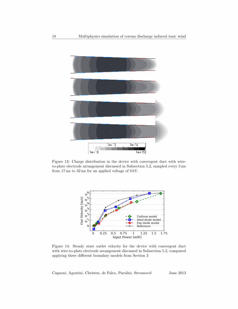
Such a loss in accuracy, though, is balanced by the better numerical per-formance. Figure 12 compares the convergence history of the iterative methodwhen the ideal diode or the exponential diode injection model is applied. Thenumber of time steps required for the electric variables to reach a stationaryregime is much higher in the case of the ideal diode condition due to the re-quirement of a smaller under-relaxation coefficient that is needed to stabilizethe method in this case. It is interesting to observe how the convergence overtime of the current to its stationary value is non-monotonic. Indeed, a possi-bly high overshoot in the current is usually observed, if the initial value of thecation density is low. In such situation, the anode contact electric field is ini-tially much higher than at steady state, and thus more intense charge injectionoccurs. An additional abrupt change in the simulated current may occur, whenthe charge present in the device, due either to the initial value or the over-shooting, is expelled from the channel as shown in Fig. 13; this abrupt changeresults in a variation of the anode charge density value, and leads to the needof a larger number of fixed point iterations. The above discussion shows that acareful choice of the initial condition is necessary in order to allow for a goodperformance of the numerical method.

Finally, Fig. 14 shows a comparison of the experimental and predicted av-erage velocities on the outlet section, plotted versus the total provided powerat the electrical steady state W = iV . The uniform model only provides anapproximation of scale of the total flow rate; on the other hand, it underes-timates both the high increase in efficiency for smaller applied power and thedrop in efficiency at higher power. The ideal diode model, on the contrary,provides a very good approximation for the efficiency of the device, due to themore realistic space distribution of the volume EHD force, even without a-prioriknowledge of the expected current. As already stated, this additional accuracycomes at the price of higher computational cost. The real diode approach, inthe end, provides a flow rate curve quite similar to the one from the uniformmodel, even if the points are biased towards the low-power region due to theunderestimation of the currents. Moreover, the approach is not dependent onempirical data, since its parameters depend mainly on the electrode radius andcould be estimated from similar cases. This result is in our opinion a fair trade-off between the need of specific empirical data on currents of the uniform model,and the excessive computational effort required by the ideal diode model.



(a) Electric field lines (grey) and electric potential isolines (black).

(b) Streamlines, sampled every 0.1 s from t = 2.6 s to t = 2.9 s.

Figure 10: Electric field (a) and air velocity (b) in the device with convergentduct with wire-to-plate electrode arrangement discussed in Subsection 5.2 at anapplied voltage of 9 kV, these results were obtained with the exponential diodeboundary condition.



Anod

e C

urre

nt [1

0-2×

mA]

02468

101214

Applied Voltage [kV]6 7 8 9 10 11

ReferenceUniform modelIdeal diode modelExp diode model

Figure 11: Anode current vs applied voltage in the device with convergent ductwith wire-to-plate electrode arrangement discussed in Subsection 5.2, computedapplying three of the boundary condition models presented in Section 3

Anode Cur. [A]Cathode Cur. [A]# Gummel Iters

Time [s]

10−5 10−4 10−3 0.01 0.1

Cu

rren

t [A

]

10−6

10−5

10−4

# Iters

0

20

80

100

(a) Exponential diode model.

Anode Cur. [A]Cathode Cur. [A]# Gummel Iters

Time [s]

0.2 0.4 0.6 0.8 1

Cu

rren

t [A

]

10−10

10−9

10−8

10−7

10−6

10−5

10−4

# Iters

0

20

80

100

(b) Ideal diode model.

Figure 12: Performance of the iterative algorithm in simulating the device withconvergent duct with wire-to-plate electrode arrangement discussed in Subsec-tion 5.2 for an applied voltage of 8 kV. The plots shows anode and cathodecurrents and the total number of iterations for the electric subsystem solutionmap E at each time step.



Figure 13: Charge distribution in the device with convergent duct with wire-to-plate electrode arrangement discussed in Subsection 5.2, sampled every 5 msfrom 17 ms to 32 ms for an applied voltage of 8 kV.

Out

Vel

ocity

[m/s

]

00.10.20.30.40.50.6

Input Power [mW]0 0.25 0.5 0.75 1 1.25 1.5 1.75

Uniform modelIdeal diode modelExp diode modelReference

Figure 14: Steady state outlet velocity for the device with convergent ductwith wire-to-plate electrode arrangement discussed in Subsection 5.2, computedapplying three different boundary models from Section 3



6 Industrial application example: an EHD cooledcondensation radiator

After the model validation carried out in Section 5, we present in this sectionan example of application of our simulation tool to the design of a cooling ap-paratus of potential impact in industrial application. In particular, we considera combination of EHD forced air convection and a two-phase thermosyphon.

Two-phase cooling, and in particular two-phase thermosyphons, have beenrecognized in being beneficial for thermal management of electronics. The us-age of pumpless systems together with dielectric fluids and high heat transfercoefficients demonstrated to be a perfect combination for cooling of electronics.

Thermosyphon condensers are commonly automotive type heat exchangers.This technology uses numerous multiport extruded tubes with capillary sizedchannels disposed in parallel and brazed to louvered air fins that meets therequired compactness. The heat removal is obtained by means of a forced airstream of air over the condenser body usually imposed by a fan element. Iffans represent a standard solution, drawbacks are commonly identified in thereliability (rotating mechanical parts), in the noise and in the occupied volume.

An EHD cooled condenser can overcome the limits of a common fan system.For a given condenser size, the EHD cooler will increase the local air speed;for a given temperature of operation of the cooler, the EHD system can enablea global reduction of the system size with reduced noise levels. Last but notleast, EHD can locally increase the condensing performances due to generatedmagnetic field enabling a reduction of the operating temperature of the electricand electronic devices.

The result we show in this section pertain to the simulation of a simplifiedmodel of EHD cooled thermosyphon, similar to the ones presented in Refs. [55,56, 57, 58]. Figure 15 depicts the geometry of the device, where the verticaltubes act as cathode and a mesh of thin wires acts as anode. The device is

Figure 15: Geometry of the thermosyphon, with the mesh of wires acting asanode, and the basic periodic cell used as computational domain.



inherently modular, so that simulation is required only for the basic periodiccell, which is in evidence in Fig. 15. On the horizontal boundary planes, periodiccondition are imposed, while on the portions of the vertical boundary planes notintersecting the solid components, symmetry conditions are enforced.

Figure 16: Cation number density (m−3) isosurfaces, for an applied voltage of10 kV.

Figure 17: Electric field lines, color scale based on log10 of the magnitude of ~Eexpressed in Vm−3, for an applied voltage of 10 kV.



Figure 16 shows the distribution of the cation density in the domain. Themaximum density is located directly in front of the pipe, and a main conductiveregion is formed. Figure 17 shows some electric field lines, which are also parallelto the EHD volume force, that triggers the fluid motion.

7 Conclusions

In this work, we studied the numerical approximation of the effects of electricdischarge on ambient air flow. First, we proposed an algorithm to deal withthe multiphysics mathematical model describing the system, by the coupling ofthe different and particular approaches already used in the fields of electronicdevice simulation and computational fluid dynamics. Furthermore, we analyzedthe particular phenomenon of corona discharge and proposed a phenomenolog-ical approach, which allows for the removal of the plasma subdomain and theelectron density conservation equation from the computation. Four differentmodels following this approach have been considered, discussed, and compared.The conclusion is that both the ideal and exponential diode models, proposedin this work, are able to reproduce the correct behavior of the corona dischargeEHD system without need of measured data for the electric current in the ac-tual device at hand. Finally, we showed how our models and algorithm can beeffectively used in a relevant industrial application.

References

[1] G. S. P. Castle, I. I. Inculet, and K. I. Burgess, IEEE Transactions onIndustry and General Applications 5, 489 (1969).

[2] K. Adamiak and P. Atten, Journal of Electrostatics 61, 85 (2004).

[3] P. Atten, A. Adamiak, B. Khaddoura, and J. L. Coulomb, Journal ofOptoelectronics and Advanced Materials 6, 1023 (2004).

[4] P. Sattari, G. S. P. Castle, and K. Adamiak, IEEE Transactions on Indus-try Applications 46, 1699 (2010).

[5] L. Zhao and K. Adamiak, in Proceedings of the Electrostatics Joint Con-ference (Boston, MA, 2009).

[6] S. O. Ahmedou and M. Havet, Journal of Electrostatics 67, 222 (2009a).

[7] S. O. Ahmedou and M. Havet, IEEE Transactions on Dielectrics and Elec-trical Insulation 16, 489 (2009b).

[8] S. O. Ahmedou, M. Havet, and O. Rouaud, Food and Bioprocess Technol-ogy 2, 240 (2009).

[9] E. Moreau and G. Touchard, Journal of Electrostatics 66, 39 (2008).



[10] R.-T. Huang, W.-J. Sheu, and C.-C. Wang, Energy Conversion and Man-agement 50, 1789 (2009).

[11] C. Kim, D. Park, K. C. Noh, and J. Hwang, Journal of Electrostatics 68,36 (2010).

[12] J. S. Chang, J. Ueno, H. Tsubone, G. D. Harvel, S. Minami, andK. Urashima, Journal of Physics D: Applied Physics 40, 5109 (2007).

[13] H. Tsubone, J. Ueno, B. Komeili, S. Minami, G. D. Harvel, K. Urashima,C. Y. Ching, and J. S. Chang, Journal of Electrostatics 66, 115 (2008).

[14] J. S. Chang, H. Tsubone, Y. N. Chun, A. A. Berezin, and K. Urashima,Journal of Electrostatics 67, 335 (2009).

[15] S. Karpov and I. Krichtafovitch, in Proceedings of the COMSOL conference(Boston, MA, 2005) pp. 399–403.

[16] N. E. Jewell-Larsen, P. Q. Zhang, C. P. Hsu, I. A. Krichtafovitch, and A. V.Mamishev, in 9th AIAA/ASME Joint Thermophysics and Heat TransferConference (2006).

[17] N. E. Jewell-Larsen, E. Tran, I. A. Krichtafovitch, and A. V. Mamishev,IEEE Transactions on Dielectrics and Electrical Insulation 13, 191 (2006b).

[18] C. P. Hsu, N. E. Jewell-Larsen, I. A. Krichtafovitch, S. W. Montgomery,J. T. Dibene II, and A. V. Mamishev, Journal of MicroelectromechanicalSystems 16, 809 (2007).

[19] N. E. Jewell-Larsen, S. V. Karpov, I. A. Krichtafovitch, V. Jayanty, C. P.Hsu, and A. V. Mamishev, in Proceedings of the ESA Annual Meeting onElectrostatics (Minneapolis, MN, 2008) pp. 1–13.

[20] N. E. Jewell-Larsen, C. P. Hsu, I. A. Krichtafovitch, S. W. Montgomery,J. T. Dibene II, and A. V. Mamishev, IEEE Transactions on Dielectricsand Electrical Insulation 15, 1745 (2008b).

[21] N. E. Jewell-Larsen, H. Ran, Y. Zhang, M. Schwiebert, and A. V. Mami-shev, in Proceedings of the Semiconductor Thermal Measurement and Man-agement Symposium, SEMI-THERM (San Jose, CA USA, 2009) pp. 1–7.

[22] D. B. Go, S. V. Garimella, and T. S. Fisher, in The Tenth IntersocietyConference on Thermal and Thermomechanical Phenomena in ElectronicsSystems, ITHERM ’06. (2006) pp. 45–53.

[23] D. B. Go, S. V. Garimella, and T. S. Fisher, Journal of Applied Physics102, 053302 (2007).

[24] T. S. Fisher, S. V. Garimella, D. B. Go, and R. K. Monja, “Various meth-ods, apparatuses, and systems that use ionic wind to affect heat transfer,”US Patent No. 7545640 (2009).


http://www.electrostatics.org/esa2008proceedings.html



[25] D. B. Go, R. A. Maturana, T. S. Fisher, and S. V. Garimella, InternationalJournal of Heat and Mass Transfer 51, 6047 (2008).

[26] D. B. Go, S. V. Garimella, T. S. Fisher, and V. Bahadur, Plasma SourcesScience and Technology 18, 035004 (2009).

[27] N. A. Kaptsov, Elektricheskie Yavleniya v Gazakz i Vakuume (OGIZ,Moscow, 1947).

[28] W. Zhang, T. S. Fisher, and S. V. Garimella, Journal of Applied Physics96, 6066 (2004).

[29] A. Yabe, Y. Mori, and K. Hijikata, AIAA Journal 16, 340 (1978).

[30] J. A. Stratton, Electromagnetic Theory (McGraw Hill, 1941).

[31] T. B. Jones, Advances in Heat Transfer 14, 107 (1979).

[32] Z. Yu, R. K. Al-Dadah, and R. H. S. Winterton, in Proceedings of theInternational Conference on Two-Phase Modelling and Experimentation,Vol. 1 (Pisa, Italy, 1999) pp. 463–472.

[33] F. W. Peek, Dielectric Phenomena in High Voltage Engineering (McGraw-Hill, New York, 1929).

[34] J. S. Townsend, Nature 62, 340 (1900).

[35] J. S. Townsend, Philosophical Magazine 1, 198 (1901).

[36] A. Aliat, C. T. Hung, C. J. Tsai, and J. S. Wu, Journal of Physics D:Applied Physics 42, 1 (2009).

[37] A. K. M. Mazumder and F. C. Lai, in Proceedings of the ESA AnnualMeeting on Electrostatics (Cleveland, OH, 2011).

[38] A. K. M. Mazumder, F. C. Lai, and X. B. Zhao, in Proceedings of the ESAAnnual Meeting on Electrostatics (Cleveland, OH, 2011).

[39] J. Zhang and F. C. Lai, in Proceedings of the ESA Annual Meeting onElectrostatics (Charlotte, NC, 2010).

[40] T. Christen and M. Seeger, Journal of Electrostatics 65, 11 (2007).

[41] L. V. Ballestra and R. Sacco, Journal of Computational Physics 195, 320(2004).

[42] F. Brezzi, L. Marini, S. Micheletti, P. Pietra, R. Sacco, and S. Wang, inNumerical Methods in Electromagnetics, Handbook of Numerical Analysis,Vol. 13, edited by W. Schilders and E. ter Maten (Elsevier, 2005) pp. 317–441.









[43] C. de Falco, R. Sacco, and G. Scrofani, Computer Methods in AppliedMechanics and Engineering 196, 1729 (2007).

[44] C. de Falco, E. Gatti, A. L. Lacaita, and R. Sacco, Journal of Computa-tional Physics 204, 533 (2005).

[45] J. Jerome, Analysis of Charge Transport: a Mathematical Study of Semi-conductor Devices (Springer-Verlag, 1996).

[46] S. Selberherr, Analysis and Simulation of Semiconductor Devices (Springer-Verlag New York, 1984).

[47] B. Chini, J. W. Jerome, and R. Sacco, in EuroSime 2006, 7th IEEE Inter-national Conference on Thermal, Mechanical and Multiphysics Simulationand Experiments in Micro-Electronics and Micro-Systems (2006) pp. 1–8.

[48] J. W. Jerome, B. Chini, M. Longaretti, and R. Sacco, Journal of Compu-tational Electronics 7, 10 (2008).

[49] J. W. Jerome and R. Sacco, Nonlinear Analysis, Theory, Methods andApplications 71, e2487 (2009).

[50] C. de Falco, J. W. Jerome, and R. Sacco, Journal of Computational Physics228, 1770 (2009).

[51] R. Issa, Journal of computational physics 62, 40 (1986).

[52] “OpenFOAM R© - The Open Source Computational Fluid Dynamics (CFD)Toolbox,” .

[53] B. Gschaider, “swak4Foam,” .

[54] C. Geuzaine and J. F. Remacle, “Gmsh: a three-dimensional finite elementmesh generator with built-in pre- and post-processing facilities,” .

[55] F. Agostini and B. Agostini, in Proceedings of the IEEE 33rd InternationalTelecommunications Energy Conference, INTELEC (2011) pp. 1–6.

[56] B. Agostini and M. Habert, in Proceedings of the 16th International HeatPipe Conference, IHPC (Lyon, France, 2012) pp. 1–6.

[57] M. Habert and B. Agostini, in Proceedings of the 16th International HeatPipe Conference, IHPC (Lyon, France, 2012) pp. 1–6.

[58] F. Agostini and L. Malinowski, in Proceedings of the 13th IEEE IntersocietyConference on Thermal and Thermomechanical Phenomena in ElectronicSystems, ITherm (2012) pp. 1077–1083.


http://www.openfoam.com

http://www.openfoam.com

http://openfoamwiki.net/index.php/Contrib/swak4Foam

http://geuz.org/gmsh

http://geuz.org/gmsh

multiphysics simulation of corona discharge induced … · multiphysics simulation of corona...

Documents