multiperiod/multiscale milp model for optimal planning of...

MULTIPERIOD/MULTISCALE MILP MODEL FOR OPTIMAL PLANNING OF ELECTRIC POWER INFRASTRUCTURES

Center for Advanced Process Decision-making CAPD Meeting, Mar. 6 – Mar 9, 2016

Cristiana L. Lara* and Ignacio E. Grossmann*

1

*Department of Chemical Engineering, Carnegie Mellon University

Electricity mix gradually shifts to lower-carbon options

2Source: EIA, Annual Energy Outlook 2015 Reference case

Electricity generation by fuel type (trillion kWh)

Renewable electricity generation by fuel type (trillion kWh)

0

30

60

90

120

2010 2020 2030 2040

Potential accelerated retirements

3

Coal-fired

Nuclear

Cumulative retirement of coal-fired generating capacity

Cumulative retirement of nuclear generating capacity

Source: EIA, Annual Energy Outlook 2014

0

30

60

90

120

2010 2020 2030 2040

Reference

High Oil and Gas Resource

Accelerated Coal and Nuclear Retirements

Accelerated Coal Retirements

0

10

20

30

40

50

2010 2020 2030 2040

Reference

Accelerated Nuclear Retirements/Accelerated Coal and Nuclear Retirements

0

10

20

30

40

50

2010 2020 2030 2040

High variability on the renewables capacity factor

• Increasing contribution of renewable power generation in the grid make it crucial to include operation details in the hourly level in long term planning models to capture their variability

4Source: U.S. Energy Information Administration, based on the Electric Reliability Council of Texas (ERCOT)

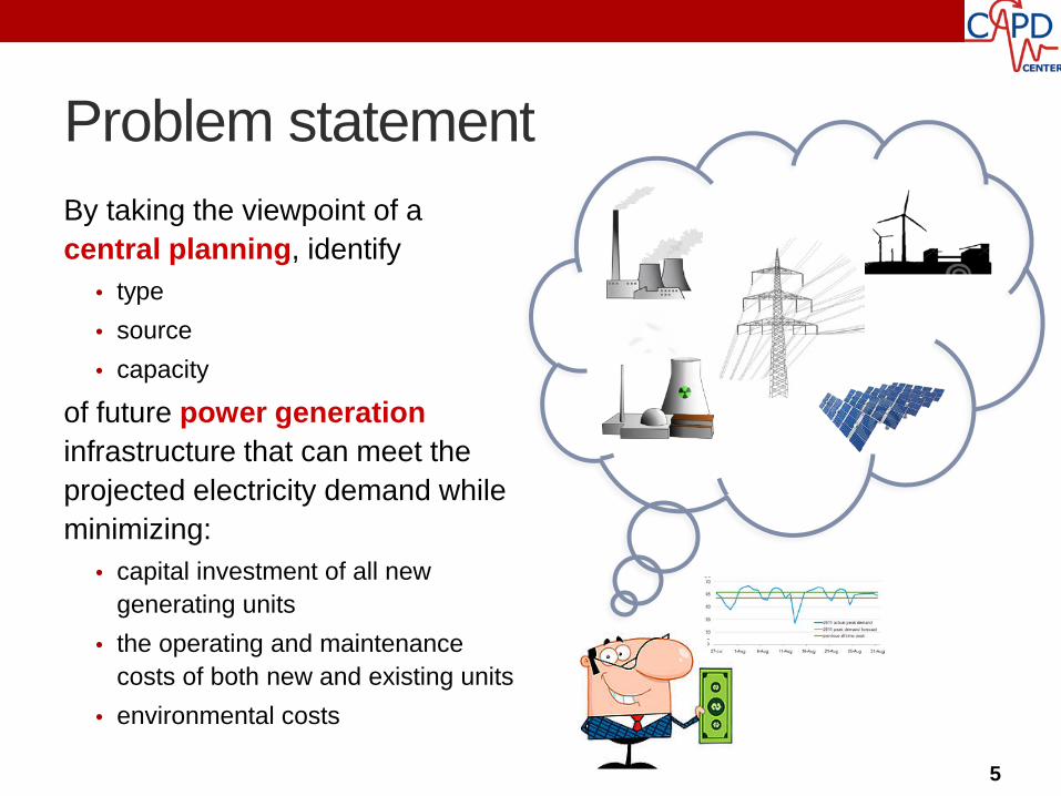
Problem statementBy taking the viewpoint of a central planning, identify

• type• source • capacity

of future power generationinfrastructure that can meet the projected electricity demand while minimizing:

• capital investment of all new generating units

• the operating and maintenance costs of both new and existing units

• environmental costs

5

Problem statementIn order to be able to capture the variability of generation by renewable source units, and assure that the load demand is met at anytime, operational decisions are also taken

• ramping limits

• unit commitment status

6

Hourly time resolution

Long term investment plans

MILP ModelObjective function: Minimization of the discounted total cost over the planning horizon comprising

• Variable operating cost• Startup cost• Fixed operating cost• Cost of investments in new capacities• Penalty for not meeting the minimum renewable annual energy production requirement

7

subject to

• Energy balance: ensures that the sum of instantaneous power equal load at all times plus a slack for potential excess generation by the renewable source generators (wind and solar)



8

subject to

• Unit minimum and maximum power output for thermal generators

Capacity nameplateMinimum % of the capacity nameplate



9

subject to

• Capacity factor for renewable source generators



10

subject to

• Minimum reserve margin requirement: ensures that the generation capacity is greater than the peak load by a predefined margin

• Minimum annual Renewable Energy Source (RES) contribution requirement: establish that if the RES quota target (imposed by environmental treaties) is not satisfied, there will be a penalty applied to the deficit in RES production



11

subject to

• Unit commitment status and ramping limits for the thermal generators

OFF OFFON

tt - 1 t + 1Startup Shutdown

Modeling strategies for MULTISCALETime scale approach

12

Spring Summer Fall Winter

Year 1, spring: Investment decisions

Year 2, spring: Investment decisionsDay Day Day Day

x 93 x 94 x 89 x 89

• Horizon: 30 years, each year has 4 periods (spring, summer, fall, winter)

• Each period is represented by one representative day on an hourly basisVarying inputs: load demand data, capacity factor of renewable source generators

• Each representative week is repeated in a cyclic manner (~3 months reduced to 1 day)

• Connection between periods: only through investment decisions

Modeling strategies for MULTISCALEClustering representation*

• Instead of representing each generator separately, aggregate same type of generators in clusters

• Decision of building/retiring and starting up/shutting down a generator switched from binary to integer variables

13

cluster

*Palmintier, B., & Webster, M. (2014). Heterogeneous unit clustering for efficient operational flexibility modeling

Case study: ERCOT region30 year time horizon

Data from ERCOT database

All costs in 2012 U$

Clusters considered:• coal-st-old1

• coal-st-old2

• ng-ct-old

• ng-cc-old

• ng-st-old

• nuc-st-old

• pv-old

• wind-old

• coal-igcc-new

• coal-igcc-ccs-new

• ng-cc-new

• ng-cc-ccs-new

• ng-ct-new

• nuc-st-new

• pv-new

• wind-new

• csp-new

14

Discrete variables: 103,050Continuous variables: 101,071Equations: 278,183CPLEX optcr = 0.05%

Considers reference* case scenario

*Based on EIA Annual Energy Outlook 2015 fuel price data

0

100

200

300

400

500

600

1 2 3 4 5 6 7 8 9 10 11 12 13 14 15 16 17 18 19 20 21 22 23 24 25 26 27 28 29 30

Pow

er g

ener

atio

n (T

W)

years

Power generation by source

coal natural gas nuclear PV wind

44%

4%18%0%

34%

Breakdown of the Total Cost

Fuel Cost*Variable Operating CostFixed Operating CostStartup CostInvestment Cost

Case study: ERCOT region

Natural gas generation will grow from 21% to 42% of the total generation

15

Minimum cost: $ 304.9 billionsOptimality gap: 0.04%CPU time: 637 s

Conclusions and Future Work• Time scale and clustering approaches reduce considerably the

size of the MILP, making it possible to solve large instances

• For ERCOT region, future investments will be focused on natural gas and wind generation

• Natural gas will be the major contributor for the overall generation by the end of the time horizon

• Future work:• Include transmission in the model (multiple generation nodes)

• Apply decomposition techniques to speed up the solution

• Address the uncertainty by extending MILP model to multi-stage MILP stochastic programming model

16

Acknowledgments

17

Funding sources:

Thank you!

multiperiod/multiscale milp model for optimal planning of...

Documents