multiparametric linear and quadratic programming - wiley-vch

3

1Multiparametric Linear and Quadratic ProgrammingNuno P. Faísca, Vivek Dua, and Efstratios N. Pistikopoulos

In this work we present an algorithm for the solution of multiparametric linearand quadratic programming problems. With linear constraints and linear or convexquadratic objective functions, the optimal solution of these optimization problemsis given by a conditional piecewise linear function of the varying parameters. Thisfunction results from first-order estimations of the analytical nonlinear optimalfunction. The core idea of the algorithm is to approximate the analytical nonlinearfunction by affine functions, whose validity is confined to regions of feasibility andoptimality. Therefore, the space of parameters is systematically characterized intodifferent regions where the optimal solution is an affine function of the parame-ters. The solution obtained is convex and continuous. Examples are presented toillustrate the algorithm and to enhance its potential in real-life applications.

1.1Introduction

Variability and uncertainty are widely recognized as crucial topics in the design andoperation of processes and systems [34]. Fluctuations in resources, market require-ments, prices, and during plant operation make imperative the study of possibleconsequences of uncertainty and variability in the feasibility and economics of aproject. In the optimization models, variability and uncertainty correspond to theinclusion of varying parameters.

According to the parameters’ description, different solving approaches have beenproposed: (i) multiperiod optimization [11, 42, 46], (ii) stochastic programming[4, 5, 10, 13, 20, 26, 40], and (iii) parametric programming. In the multiperiod op-timization approach, the time horizon is discretized into time periods, associatedwith forecasts of the parameters. For instance, if the forecast is a demand of aspecific chemical product in the ensuing years, the objective is to find a planningstrategy for producing these chemicals, which maximizes the net present value.If the probability distribution function of the parameters is known, the stochasticprogramming identifies the optimal solution which corresponds to the maximum

Multi-Parametric Programming. Edited by E. Pistikopoulos, M. Georgiadis, and V. DuaCopyright © 2007 WILEY-VCH Verlag GmbH & Co. KGaA, WeinheimISBN: 978-3-527-31691-5

4 1 Multiparametric Linear and Quadratic Programming

Fig. 1.1 Crude oil refinery.

expected profit. At last, the parametric programming approach aims to obtain theoptimal solution as an explicit function of the parameters. In this chapter we willdiscuss techniques based upon the fundamentals of parametric programming.

Parametric programming is based on the sensitivity analysis theory, distinguish-ing from the latter in the targets. Sensitivity analysis provides solutions in theneighborhood of the nominal value of the varying parameters, whereas parametricprogramming provides a complete map of the optimal solution in the space of thevarying parameters. Theory and algorithms for the solution of a wide range of para-metric programming problems have been reported in the literature [1, 3, 15–18, 22,25, 33, 45].

�Example 1 [19]A refinery blending and production process is depicted in Fig. 1.1. The ob-jective of the company is to maximize the profit by selecting the optimalcombination of raw materials and products. Operating conditions are pre-sented in Table 1.1, where θ1 and θ2 are parameters representing an ad-ditional maximum allowable production of gasoline and kerosene, respec-tively.This problem formulates as a multiparametric linear programming prob-lem (1.1), where x1 and x2 are the flow rates of the crude oils 1 and 2 inbbl/day, respectively, and the units of profit are $/day.

Profit = maxx

8.1x1 + 10.8x2, (1.1a)

s.t. 0.80x1 + 0.44x2 ≤ 24 000 + θ1, (1.1b)

0.05x1 + 0.10x2 ≤ 2000 + θ2, (1.1c)

Table 1.1 Refinery data.

Volume % yield Maximum allowableCrude 1 Crude 2 production (bbl/day)

Gasoline 80 44 24 000 + θ1Kerosene 5 10 2000 + θ2Fuel oil 10 36 6000Residual 5 10 –Processing cost ($/bbl) 0.50 1.00 –

1.1 Introduction 5

0.10x1 + 0.36x2 ≤ 6000, (1.1d)

x1 ≥ 0, x2 ≥ 0, (1.1e)

0 ≤ θ1 ≤ 6000, (1.1f)

0 ≤ θ2 ≤ 500. (1.1g)

The importance of solving this problem is as follows:(i) the optimal policy for selecting the crude oil source is

known as a function of θ1 and θ2;(ii) substituting the value of θ1 and θ2 into the parametric

profiles we know directly the optimal profit;(iii) the sensitivity of the profit to the parameters is

identified. The board of the company foresees moresensitive operating regions, making the managementmore efficient.

�Example 2 [12]A Dutch agriculture cooperative society has to deal with the excess of milkproduced. Since some high-valued products can be processed, this coop-erative society has to set either the quantities, taking into account the de-mand (z), and prices (x) for each product. This specific cooperative societyconsiders but four types of products: milk for direct consumption, butter,fat cheese, and low fat cheese (Fig. 1.2).The capacity constraints are

0.026z1 + 0.800z2 + 0.306z3 + 0.245z4 ≤ 119, (1.2a)

0.086z1 + 0.020z2 + 0.297z3 + 0.371z4 ≤ 251, (1.2b)

z1 ≥ 0, (1.2c)

z2 ≥ 0, (1.2d)

z3 ≥ 0, (1.2e)

z4 ≥ 0. (1.2f)

Obviously, consumer demand depends critically on the price of the product,where a negative relation is expected:

Fig. 1.2 Possible products from the milk surplus.


z1 = –1.2338x1 + 2139 + w1, (1.3a)

z2 = –0.0203x2 + 135 + w2, (1.3b)

z3 = –0.0136x3 + 0.0015x4 + 103 + w3, (1.3c)

z4 = +0.0016x3 – 0.0027x4 + 19 + w4, (1.3d)

where w1, w2, w3, and w4 are uncertainties associated with the consumerdemand.The cooperative society wants to reward as much as possible their associates,and hence the objective is to maximize profit. Ignoring production costs, theobjective function is written as

Profit = maxx

4∑i=1

xi · zi, (1.4)

which is a quadratic function of prices, xi. The government avoids the esca-lation of the prices with an extra policy constraint:

0.0163x1 + 0.0003x2 + 0.0006x3 + 0.0002x4 ≤ 10 + k, (1.5)

where k refers to a possible price rise (e.g., k = 0.1 means a rise of 1% onthe overall prices). This is regarded as a social constraint.

The optimization problem formulates as in (1.6).

Profit = maxx1,x2,x3,x4

4∑i=1

xi · zi,

s.t. 0.026z1 + 0.800z2 + 0.306z3 + 0.245z4 ≤ 119,

0.086z1 + 0.020z2 + 0.297z3 + 0.371z4 ≤ 251,

0.0163x1 + 0.0003x2 + 0.0006x3 + 0.0002x4 ≤ 10 + k,

z1 = –1.2338x1 + 2139 + w1,

z2 = –0.0203x2 + 135 + w2,

z3 = –0.0136x3 + 0.0015x4 + 103 + w3,

z4 = +0.0016x3 – 0.0027x4 + 19 + w4,

z1 ≥ 0,

z2 ≥ 0,

z3 ≥ 0,

z4 ≥ 0,

–150 ≤ w1 ≤ 150,

–5 ≤ w2 ≤ 5,

–6 ≤ w3 ≤ 6,

–2 ≤ w4 ≤ 2,

–1 ≤ k ≤ 1.

(1.6)

1.2 Methodology 7

The significance of such solution is as follows:(i) the optimal price policy is known as a function of the

uncertainty in the demand, wi, and possible price rise, k;(ii) sensitivity of the current best decision is known, and

supports an efficient decision making.

As shown, this type of information is very useful for solving reactive or onlineoptimization problems. Such problems usually require a repetitive solution of op-timization problems; due to the varying conditions of most processes, the optimaldecision/action changes with time. The key advantage of parametric programmingis to obtain the optimal solution as a function of the varying parameters withoutexhaustively enumerating the entire parametric space.

A broad spectrum of process engineering applications has been identified: (i) hy-brid parametric/stochastic programming [2, 27], (ii) process planning under uncer-tainty [35], (iii) scheduling under uncertainty [41], (iv) material design under uncer-tainty [14], (v) multiobjective optimization [31, 32, 39], (vi) flexibility analysis [6, 8],and (vii) computation of singular multivariate normal probabilities [7]. Althoughparametric programming has various applications, the online control problem [9,37, 38, 44] is the most prolific application, where control variables are obtained as afunction of the initial state of the system. This reduces the real-time optimal controlproblem to a simple function evaluation problem. Mathematically, such problemsare formulated as multiparametric quadratic programs (mp-QP). Robust onlinecontrol problems that can take into account uncertainty and disturbance can alsobe reformulated as mp-QPs to obtain the explicit robust control law [28, 29, 43].

The rest of the chapter organizes as follows. Section 1.2 describes the underlyingmathematical background of the methodology, and finalizes with the algorithm;convexity/continuity properties of the solution are also proven. In section 1.3, someexamples are solved in order to illustrate the procedure and to give an insight ofthe complexity involved.

1.2Methodology

Consider the general parametric nonlinear programming problem:

minx

f(x, θ ),

s.t. gi(x, θ ) ≤ 0, ∀ i = 1, . . . , p,hj(x, θ ) = 0, ∀ j = 1, . . . , q,x ∈ X ⊆ R

n,θ ∈ � ⊆ R

m,

(1.7)

where f, g, and h are twice continuously differentiable in x and θ . The first-orderKarush–Kuhn–Tucker (KKT) optimality conditions for (1.7) are given as follows:


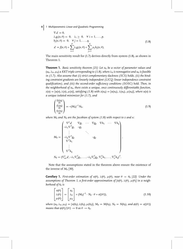
∇L = 0,λigi(x, θ ) = 0, λi ≥ 0, ∀ i = 1, . . . , p,hj(x, θ ) = 0, ∀ j = 1, . . . , q,

L = f(x, θ ) +p∑

i=1

λigi(x, θ ) +q∑

j=1

µjhj(x, θ ).

(1.8)

The main sensitivity result for (1.7) derives directly from system (1.8), as shown inTheorem 1.

Theorem 1. Basic sensitivity theorem [21]: Let x0 be a vector of parameter values and(u0, λ0, µ0) a KKT triple corresponding to (1.8), where λ0 is nonnegative and u0 is feasiblein (1.7). Also assume that (i) strict complementary slackness (SCS) holds, (ii) the bind-ing constraint gradients are linearly independent (LICQ: linear independence constraintqualification), and (iii) the second-order sufficiency conditions (SOSC) hold. Then, inthe neighborhood of x0, there exists a unique, once continuously differentiable function,z(x) = [u(x), λ(x), µ(x)], satisfying (1.8) with z(x0) = [u(x0), λ(x0), µ(x0)], where u(x) isa unique isolated minimizer for (1.7), and

du(x0)

dxdλ(x0)

dxdµ(x0)

dx

= –(M0)–1N0, (1.9)

where M0 and N0 are the Jacobian of system (1.8) with respect to z and x:

M0 =

∇2L ∇g1 · · · ∇gp ∇h1 · · · ∇hq

–λ1∇Tg1 –g1...

. . .–λp∇Tgp –gp

∇Th1...

∇Thq

,

N0 = (∇2xuL, –λ1∇T

x g1, . . . , –λp∇Tx gp, ∇T

x h1, . . . , ∇Tx hq)T.

Note that the assumptions stated in the theorem above ensure the existence ofthe inverse of M0 [30].

Corollary 1. First-order estimation of x(θ ), λ(θ ), µ(θ ), near θ = θ0 [22]: Under theassumptions of Theorem 1, a first-order approximation of [x(θ ), λ(θ ), µ(θ )] in a neigh-borhood of θ0 is

x(θ )λ(θ )µ(θ )

=

x0

λ0

µ0

+ (M0)–1 · N0 · θ + o(‖θ‖), (1.10)

where (x0, λ0, µ0) = [x(θ0), λ(θ0), µ(θ0)], M0 = M(θ0), N0 = N(θ0), and φ(θ ) = o(‖θ‖)means that φ(θ )/‖θ‖ → 0 as θ → θ0.

1.2 Methodology 9

Despite being a simple and linear expression, Eq. (1.10) may lead to complexcomputational problems, since in the general nonlinear case the Jacobians of sys-tem (1.8) are in most of the cases complex. Fortunately, it simplifies when (1.7) hasa quadratic objective function, linear constraints, and the parameters appear on theright-hand side of the constraints:

z(θ ) = minx

cTx + 12 xTQx,

s.t. Ax ≤ b + Fθ ,x ∈ X ⊆ R

n,θ ∈ � ⊆ R

m,

(1.11)

where c is a constant vector of dimension n, Q is an (n × n) symmetric positivedefinite constant matrix, A is a (p × n) constant matrix, F is a (p × m) constantmatrix, b is a constant vector of dimension p, and X and � are compact polyhedralconvex sets of dimensions n and m, respectively. Note that a term of the form θTPxin the objective function can also be addressed in the above formulation, as it canbe transformed into the form given in (1.11) by substituting x = s – Q–1PTθ , wheres is a vector of arbitrary variables of dimension n and P is a constant matrix ofdimension (m × n).

An application of Theorem 1 to (1.11) at [x(θQ), θQ] gives the following result: dx(θQ)

dθ

dλ(θQ)dθ

= –(MQ)–1NQ, (1.12)

where

MQ =

Q AT1 · · · AT

p

–λ1A1–V1...

. . .–λpAp –Vp

,

NQ = [Y, λ1F1, . . . , λpFp]T,

Vi = Aix(θQ) – bi – FiθQ,

(1.13)

and Y is a null matrix of dimension (n×m). Thus, in the linear–quadratic optimiza-tion problem, the Jacobians reduce to a mere algebraic manipulation of the matri-ces declared in (1.11). In the neighborhood of the KKT point, [x(θQ), θQ], Corollary 1writes as follows:[

xQ(θ )λQ(θ )

]= –(MQ)–1NQ(θ – θQ) +

[x(θQ)λ(θQ)

]. (1.14)

Note that when assumptions in Theorem 1 are respected MQ is always invertible.This is where parametric programming detaches from the sensitivity analysis

theory. Whilst sensitivity analysis stops here, where we know what happens if theprocess conditions deviate from the nominal values to some value in its neigh-borhood, parametric programming is concerned with the whole range of the para-metric variability. The former associates with the uncertainty and the latter to thevariability of the process.


The space of θ where this solution (1.14) remains optimal is defined as the criticalregion, CRQ, and can be obtained by using feasibility and optimality conditions.Note that for convenience and simplicity in presentation, we use the notation CRto denote the set of points in the space of θ that lie in CR as well as to denote theset of inequalities which define CR. Feasibility is ensured by substituting xQ(θ ) intothe inactive inequalities given in (1.11), whereas the optimality condition is givenby λQ(θ ) ≥ 0, where λQ(θ ) corresponds to the vector of active inequalities, resultingin a set of parametric constraints. Let this set be represented by

CRR = {AxQ(θ ) ≤ b + Fθ , λQ(θ ) ≥ 0, CRIG}, (1.15)

where A, b, and F correspond to the inactive inequalities and CRIG represents aset of linear inequalities defining an initial given region. From the parametric in-equalities thus obtained, the redundant inequalities are removed and a compactrepresentation of CRQ is obtained as follows:

CRQ = �{CRR}, (1.16)

where � is an operator which removes redundant constraints—for a procedure toidentify redundant constraints see [25] (see Appendix A for a summary). Note thata CRQ is a polyhedral region. Once CRQ has been defined for a solution, [x(θQ), θQ],the next step is to define the rest of the region, CRrest, as proposed in [16] (seeAppendix B for a summary):

CRrest = CRIG – CRQ. (1.17)

Another set of parametric solutions in each of these regions is then obtainedand corresponding CRs are obtained. The algorithm terminates when there are nomore regions to be explored. In other words, the algorithm terminates when thesolution of the differential equation (1.12) has been fully approximated by first-order expansions.

The main steps of the algorithm are outlined in Table 1.2. Note that while defin-ing the rest of the regions, some of the regions are split and hence the same optimal

Table 1.2 mp-QP algorithm.

Step 1 In a given region solve (1.11) by treating θ as a free variable to obtaina feasible point [θQ]

Step 2 Fix θ = θQ and solve (1.11) to obtain [x(θQ), λ(θQ)]

Step 3 Compute [–(MQ)–1NQ] from (1.12)

Step 4 Obtain [xQ(θ ), λQ(θ )] from (1.14)

Step 5 Form a set of inequalities, CRR, as described in (1.15)

Step 6 Remove redundant inequalities from this set of inequalities and de-fine the corresponding CRQ as given in (1.16)

Step 7 Define the rest of the region, CRrest as given in (1.17)

Step 8 If no more regions to explore, go to next step, otherwise go to Step 1

Step 9 Collect all the solutions and unify the regions having the same solu-tion to obtain a compact representation

1.2 Methodology 11

solution may be obtained in more than one regions. Therefore, the regions with thesame optimal solution are united and a compact representation of the final solutionis obtained.

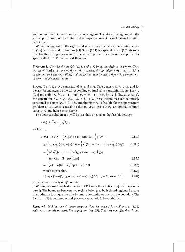
When θ is present on the right-hand side of the constraints, the solution spaceof (1.7) is convex and continuous [23]. Since (1.11) is a special case of (1.7), its solu-tion has these properties as well. Due to its importance, we prove these propertiesspecifically for (1.11) in the next theorem.

Theorem 2. Consider the mp-QP (1.11) and let Q be positive definite, � convex. Thenthe set of feasible parameters �f ⊆ � is convex, the optimizer x(θ ) : �f → R

n iscontinuous and piecewise affine, and the optimal solution z(θ ) : �f → R is continuous,convex, and piecewise quadratic.

Proof. We first prove convexity of �f and z(θ ). Take generic θ1, θ2 ∈ �f and letz(θ1), z(θ2) and x1, x2 be the corresponding optimal values and minimizers. Let α ∈[0, 1] and define xα � αx1 + (1 – α)x2, θα � αθ1 + (1 – α)θ2. By feasibility, x1, x2 satisfythe constraints Ax1 ≤ b + Fθ1, Ax2 ≤ b + Fθ2. These inequalities can be linearlycombined to obtain Axα ≤ b + Fθα and therefore xα is feasible for the optimizationproblem (1.11). Since a feasible solution, x(θα), exists at θα , an optimal solutionexists at θα and hence �f is convex.

The optimal solution at θα will be less than or equal to the feasible solution:

z(θα) ≤ cTxα +12

xTαQxα

and hence,

z (θα) – [α(cTx1 +12

xT1 Qx1) + (1 – α)(cTx2 +

12

xT2 Qx2)] (1.18a)

≤ cTxα +12

xTαQxα – [α(cTx1 +

12

xT1 Qx1) + (1 – α)(cTx2 +

12

xT2 Qx2)] (1.18b)

= 12

[α2xT1 Qx1 + (1 – α)2xT

2 Qx2 + 2α(1 – α)xT2 Qx1

– αxT1 Qx1 – (1 – α)xT

2 Qx2] (1.18c)

= –12α(1 – α)(x1 – x2)TQ(x1 – x2) ≤ 0, (1.18d)

which means that, (1.18e)

z(αθ1 + (1 – α)θ2) ≤ αz(θ1) + (1 – α)z(θ2), ∀θ1, θ2 ∈ �, ∀α ∈ [0, 1], (1.18f)

proving the convexity of z(θ ) on �f.Within the closed polyhedral regions, CRQ, in �f the solution x(θ ) is affine (Corol-

lary 1). The boundary between two regions belongs to both closed regions. Becausethe optimum is unique the solution must be continuous across the boundary. Thefact that z(θ ) is continuous and piecewise quadratic follows trivially.

Remark 1. Multiparametric linear program: Note that when Q is a null matrix, (1.11)reduces to a multiparametric linear program (mp-LP). This does not affect the solution


procedure described above and the algorithm remains the same. This is because the re-sults presented in the theorems are still valid as explained next. The results presented inTheorem 1 continue to hold true and SOSC is valid in spite of the fact that Q is a nullmatrix as discussed on page 71 in [22]. For mp-LPs x is an affine function of θ and λ

remains constant in a CR as shown in Chapter 4 in [25] and therefore Corollary 1 can beused. Whilst the results of Theorem 2 regarding �f and x(θ ) are still valid, z(θ ) simplifiesto a continuous, convex, and piecewise linear function of θ as also shown in Chapter 4in [25].

Hence, at the end of the algorithm the solution obtained is a conditional piece-wise function of the parameters and Theorem 2 implies that the optimal functioncomputed, z(θ ), is continuous and convex.

1.3Numerical Examples

In this section, the solution steps are described in detail for the two illustrativeexamples presented before: the refinery problem and the surplus milk production.Additionally, we solve a mp-QP problem corresponding to a model-based predictivecontrol problem [37].

1.3.1Example 1: Crude Oil Refinery

Consider the mp-LP problem formulated for the crude oil refinery example:

Profit = maxx

8.1x1 + 10.8x2, (1.19a)

s.t. 0.80x1 + 0.44x2 ≤ 24 000 + θ1, (1.19b)

0.05x1 + 0.10x2 ≤ 2000 + θ2, (1.19c)

0.10x1 + 0.36x2 ≤ 6000, (1.19d)

x1 ≥ 0, (1.19e)

x2 ≥ 0, (1.19f)

0 ≤ θ1 ≤ 6000, (1.19g)

0 ≤ θ2 ≤ 500. (1.19h)

The solutions steps are as follows.

Step 1. Solve (1.19) by treating θ1 and θ2 as free variables. Afeasible point obtained is θQ–1 = [0, 0]T;

Step 2. Fix θQ–1 = [0, 0]T and solve (1.19). The solution is:xQ–1 = [26 207, 6896.6]T; λQ–1 = [4.655, 87.52, 0];

1.3 Numerical Examples 13

Step 3. Compute [–M–1Q–1NQ–1] from (1.13). The solution is given by

–M–1Q–1NQ–1 =

1.724 –7.586–0.8621 13.790.0000 0.00000.0000 0.00000.0000 0.0000

.

Step 4. Compute [xQ–1(θ ), λQ–1(θ )] from (1.14):

x1Q–1(θ )

x2Q–1(θ )

λ1Q–1(θ )

λ2Q–1(θ )

λ3Q–1(θ )

=

1.724 –7.586–0.8621 13.790.0000 0.00000.0000 0.00000.0000 0.0000

· (θ – θQ1 ) +

26 2076896.64.55287.52

0.0000

,

or,

x1Q–1 = 1.724 · θ1 – 7.586 · θ2 + 26207,

x2Q–1 = –0.8621 · θ1 + 13.79 · θ2 + 6896.6,

λ1Q–1 = 4.555,

λ2Q–1 = 87.52,

λ3Q–1 = 0.0000.

Step 5. Form a set of inequalities corresponding to CRR,

CRR =

AxQ–1(θ ) ≤ b + Fθ : –0.1380θ1 + 4.206θ2 ≤ 896.5,

λQ–1(θ ) ≥ 0 :

4.552 ≥ 0,87.52 ≥ 0,0.0000 ≥ 0,

CRIG :

{0 ≤ θ1 ≤ 6000,0 ≤ θ2 ≤ 500,

(1.20)

Step 6. Remove redundant constraints,

CRrest =

–0.1380θ1 + 4.206θ2 ≤ 896.5,0 ≤ θ1 ≤ 6000,0 ≤ θ2.

(1.21)

Step 7. Define the rest of the region, CRrest,

CRR =

–0.1380θ1 + 4.206θ2 ≥ 896.5,0 ≤ θ1 ≤ 6000,θ2 ≤ 500.

(1.22)


Table 1.3 Solution of the refinery example.

i CRi Optimal solution

1 –0.14θ1 + 4.21θ2 ≤ 896.55 Profit(θ ) = 4.66θ1 + 87.52θ2 + 286 758.60 ≤ θ1 ≤ 6000 x1 = 1.72θ1 – 7.59θ2 + 26 206.900 ≤ θ2 x2 = –0.86θ1 + 13.79θ2 + 6896.55

2 –0.14θ1 + 4.21θ2 ≥ 896.55 Profit(θ ) = 7.53θ1 + 305 409.840 ≤ θ1 ≤ 6000 x1 = 1.48θ1 + 24 590.16θ2 ≤ 500 x2 = –0.41θ1 + 9836.07

Step 8. There is a region to explore, region (1.22). Return to Step 1and include constraints (1.22) in the optimizationproblem (1.19). This problem terminates in the nextiteration ending with two critical regions.

Step 9. Collect the two regions. Since they have different solutions,they are not merged.

The solution of this problem is given in Table 1.3 and Fig. 1.3.We can conclude the following:(i) A complete map of all the optimal solutions, profit and crude

oil flowrates as a function of θ1 and θ2, is available.(ii) The space of θ1 and θ2 has been divided into two regions,

CR1 and CR2, where the profiles of profit and flowrates ofcrude oils remain optimal and hence (a) one does not have toexhaustively enumerate the complete space of θ1 and θ2 and(b) the optimal solution can be obtained by simplysubstituting the value of θ1 and θ2 into the parametricprofiles without any further optimization calculations.

Fig. 1.3 Solution of refinery example.

1.3 Numerical Examples 15

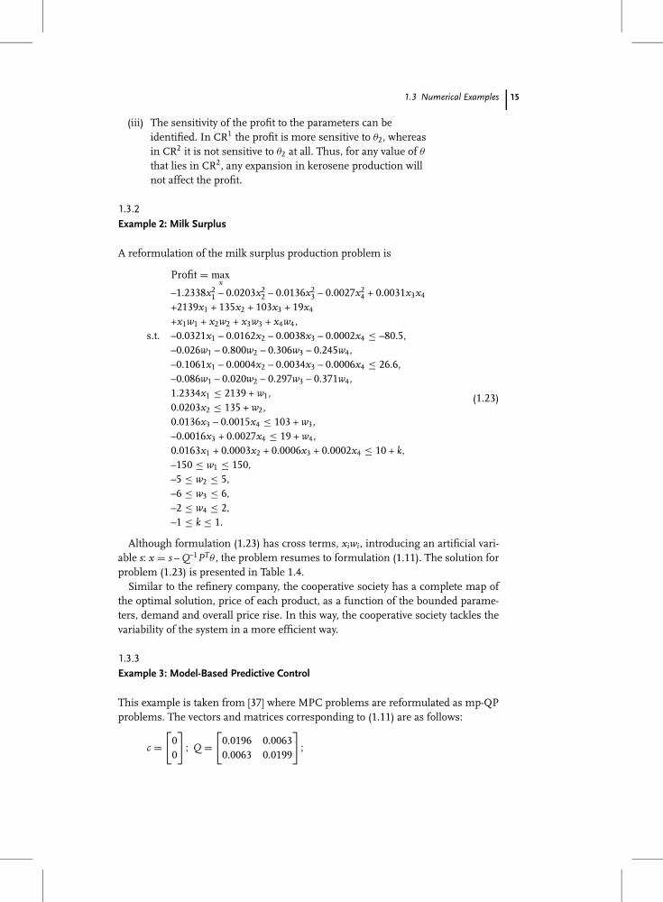
(iii) The sensitivity of the profit to the parameters can beidentified. In CR1 the profit is more sensitive to θ2, whereasin CR2 it is not sensitive to θ2 at all. Thus, for any value of θ

that lies in CR2, any expansion in kerosene production willnot affect the profit.

1.3.2Example 2: Milk Surplus

A reformulation of the milk surplus production problem is

Profit = maxx

–1.2338x21 – 0.0203x2

2 – 0.0136x23 – 0.0027x2

4 + 0.0031x3x4

+2139x1 + 135x2 + 103x3 + 19x4

+x1w1 + x2w2 + x3w3 + x4w4,s.t. –0.0321x1 – 0.0162x2 – 0.0038x3 – 0.0002x4 ≤ –80.5,

–0.026w1 – 0.800w2 – 0.306w3 – 0.245w4,–0.1061x1 – 0.0004x2 – 0.0034x3 – 0.0006x4 ≤ 26.6,–0.086w1 – 0.020w2 – 0.297w3 – 0.371w4,1.2334x1 ≤ 2139 + w1,0.0203x2 ≤ 135 + w2,0.0136x3 – 0.0015x4 ≤ 103 + w3,–0.0016x3 + 0.0027x4 ≤ 19 + w4,0.0163x1 + 0.0003x2 + 0.0006x3 + 0.0002x4 ≤ 10 + k,–150 ≤ w1 ≤ 150,–5 ≤ w2 ≤ 5,–6 ≤ w3 ≤ 6,–2 ≤ w4 ≤ 2,–1 ≤ k ≤ 1.

(1.23)

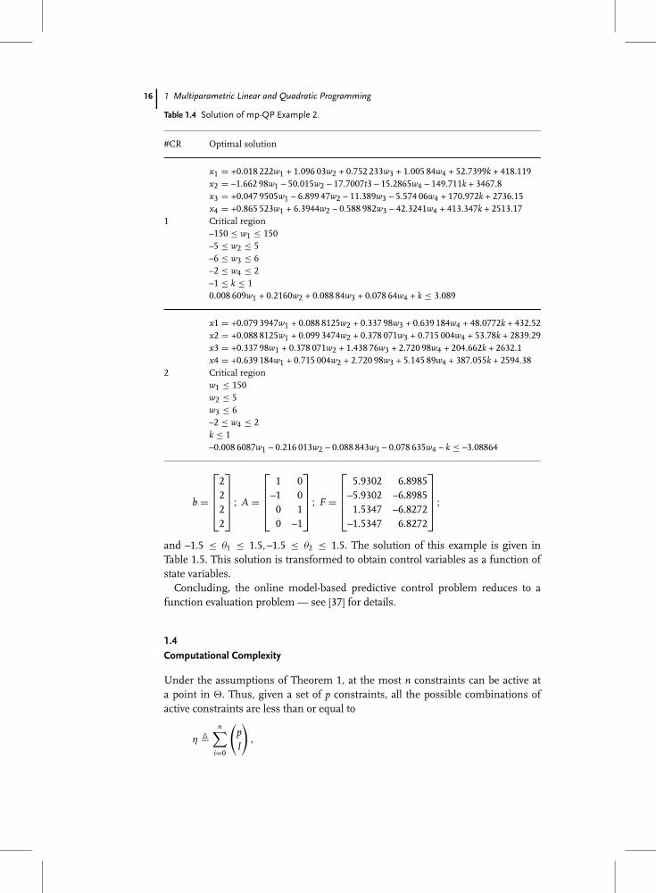
Although formulation (1.23) has cross terms, xiwi, introducing an artificial vari-able s: x = s – Q–1PTθ , the problem resumes to formulation (1.11). The solution forproblem (1.23) is presented in Table 1.4.

Similar to the refinery company, the cooperative society has a complete map ofthe optimal solution, price of each product, as a function of the bounded parame-ters, demand and overall price rise. In this way, the cooperative society tackles thevariability of the system in a more efficient way.

1.3.3Example 3: Model-Based Predictive Control

This example is taken from [37] where MPC problems are reformulated as mp-QPproblems. The vectors and matrices corresponding to (1.11) are as follows:

c =[

00

]; Q =

[0.0196 0.00630.0063 0.0199

];


Table 1.4 Solution of mp-QP Example 2.

#CR Optimal solution

x1 = +0.018 222w1 + 1.096 03w2 + 0.752 233w3 + 1.005 84w4 + 52.7399k + 418.119x2 = –1.662 98w1 – 50.015w2 – 17.7007t3 – 15.2865w4 – 149.711k + 3467.8x3 = +0.047 9505w1 – 6.899 47w2 – 11.389w3 – 5.574 06w4 + 170.972k + 2736.15x4 = +0.865 523w1 + 6.3944w2 – 0.588 982w3 – 42.3241w4 + 413.347k + 2513.17

1 Critical region–150 ≤ w1 ≤ 150–5 ≤ w2 ≤ 5–6 ≤ w3 ≤ 6–2 ≤ w4 ≤ 2–1 ≤ k ≤ 10.008 609w1 + 0.2160w2 + 0.088 84w3 + 0.078 64w4 + k ≤ 3.089

x1 = +0.079 3947w1 + 0.088 8125w2 + 0.337 98w3 + 0.639 184w4 + 48.0772k + 432.52x2 = +0.088 8125w1 + 0.099 3474w2 + 0.378 071w3 + 0.715 004w4 + 53.78k + 2839.29x3 = +0.337 98w1 + 0.378 071w2 + 1.438 76w3 + 2.720 98w4 + 204.662k + 2632.1x4 = +0.639 184w1 + 0.715 004w2 + 2.720 98w3 + 5.145 89w4 + 387.055k + 2594.38

2 Critical regionw1 ≤ 150w2 ≤ 5w3 ≤ 6–2 ≤ w4 ≤ 2k ≤ 1–0.008 6087w1 – 0.216 013w2 – 0.088 843w3 – 0.078 635w4 – k ≤ –3.08864

b =

2222

; A =

1 0–1 00 10 –1

; F =

5.9302 6.8985–5.9302 –6.89851.5347 –6.8272

–1.5347 6.8272

;

and –1.5 ≤ θ1 ≤ 1.5, –1.5 ≤ θ2 ≤ 1.5. The solution of this example is given inTable 1.5. This solution is transformed to obtain control variables as a function ofstate variables.

Concluding, the online model-based predictive control problem reduces to afunction evaluation problem — see [37] for details.

1.4Computational Complexity

Under the assumptions of Theorem 1, at the most n constraints can be active ata point in �. Thus, given a set of p constraints, all the possible combinations ofactive constraints are less than or equal to

η �n∑

i=0

(pI

),

1.4 Computational Complexity 17

Table 1.5 Solution of mp-QP Example 2: x(θ)i = Wiθ + wi, CRi : �iθ ≤ φi.

W1 =[

+0.000 000 +0.000 000+0.000 000 +0.000 000

]w1 =

[+0.000 000+0.000 000

]

�1 =

–1.0000 –1.16331.0000 1.1633

–1.0000 4.44861.0000 –4.4486

φ1 =

0.33730.33731.30321.3032

W2 =[

5.9302 6.89851.5347 –6.8272

]w2 =

[2.0000

–2.0000

]

�2 =

–1.0000 00 –1.0000

1.3655 1.0000–1.0000 1.3608

φ2 =

1.50001.5000

–0.2885–0.4006

W3 =[

–0.4933 2.19451.5347 –6.8272

]w3 =

[0.6429

–2.0000

]

�3 =

0 –1.0000–1.3655 –1.0000

1.0000 01.3655 1.0000

–1.0000 4.4486

φ3 =

1.50000.28851.50000.5618

–1.3032

W4 =[

5.9302 6.8985–1.8774 –2.1839

]w4 =

[2.0000

–0.6332

]

�4 =

–1.0000 0–1.0000 1.3608

1.0000 –1.36081.0000 1.1633

φ4 =

1.50000.77170.4006

–0.3373

W5 =[

5.9302 6.89851.5347 –6.8272

]w5 =

[2.00002.0000

]

�5 =[

–1.0000 01.0000 –1.36081.3655 1.0000

]φ5 =

[1.5000

–0.7717–0.5618

]

W6 =[

5.9302 6.89851.5347 –6.8272

]w6 =

[–2.0000

2.0000

]

�6 =

1.0000 00 1.0000

–1.3655 –1.00001.0000 –1.3608

φ6 =

1.50001.5000

–0.2885–0.4006

W7 =[

–0.4933 2.19451.5347 –6.8272

]w7 =

[–0.6429

2.0000

]

�7 =

0 1.00001.3655 1.0000

–1.0000 0–1.3655 –1.0000

1.0000 –4.4486

φ7 =

1.50000.28851.50000.5618

–1.3032

W8 =[

5.9302 6.8985–1.8774 –2.1839

]w8 =

[–2.0000

0.6332

]

�8 =

1.0000 0–1.0000 1.3608

1.0000 –1.3608–1.0000 –1.1633

φ8 =

1.50000.40060.7717

–0.3373

W9 =[

5.9302 6.89851.5347 –6.8272

]w9 =

[–2.0000–2.0000

]

�9 =[

1.0000 0–1.0000 1.3608–1.3655 –1.0000

]φ9 =

[1.5000

–0.7717–0.5618

]


where(pi

)= p!

(p – i)!i!.

In the worst case, an estimate of ηr, the number of regions, CR, generated canbe obtained as follows. The following analysis does not take into account (i) thereduction of redundant constraints, and (ii) possible empty sets are not further par-titioned. The first critical region, CRQ is defined by the constraints given in (1.15).For simplicity assume that CRIG is unbounded. Thus, first CRQ is defined by pconstraints. From Appendix B, CRrest consists of p convex polyhedra CRl definedby at most p inequalities. For each CRl, a new CR is determined which consists of2p inequalities (the additional p inequalities come from the condition CR ⊆ CRl),and therefore the corresponding CRrest partition includes 2p sets defined by 2p in-equalities. This way of generating regions can be associated with a search tree. Byinduction, it is easy to prove that at the tree level k + 1 there are k!pk regions definedby (k + 1)p constraints. As observed earlier, each CR is the largest set correspond-ing to a certain combination of active constraints. Therefore, the search tree has amaximum depth of η, as at each level there is one admissible combination less. In

conclusion, the number of regions is ηr ≤η–1∑k=0

k!pk, each one defined by at most ηp

linear inequalities.The algorithm has been fully automated [36] and tested on a number of prob-

lems. The computational experience with test problems on a Pentium II-300 MHzcomputer is given in Tables 1.6 and 1.7.

Table 1.6 Computation time (seconds).

p n/m 2 3 4 5

4 2 3.02 4.12 5.05 5.33

6 3 10.44 26.75 31.7 70.19

8 4 25.27 60.20 53.93 58.61

Table 1.7 Number of regions.

p n/m 2 3 4 5

4 2 7 7 7 7

6 3 17 47 29 43

8 4 29 99 121 127

1.5 Concluding Remarks 19

1.5Concluding Remarks

A sensitivity analysis based algorithm has been presented for the solution of multi-parametric linear and quadratic problems. These optimization problems have lin-ear or convex quadratic objective function and linear constraints; the varying para-meters are assumed to be additive linear terms on the constraints’ right-hand side.Through a systematic partition of the parametric space, the algorithm provides acomplete map of the optimal solution as a conditional piecewise linear functionof the parameters. Each piecewise function derives from first-order estimation ofthe analytical nonlinear optimal function. Therefore, the piecewise linear functionsare valid inside characteristic regions, defined using the optimality and feasibilityconditions. Hence, the core idea of the algorithm is to approximate the analyti-cal nonlinear function by affine functions, whose validity is optimally confined tocritical regions. The solution obtained is convex and continuous.

In the context of online optimization, online model-based control and optimiza-tion problems involving parametric uncertainty can be reformulated as multipara-metric optimization programs. Optimal control actions are computed off-line asfunctions of the state variables, and the space of state variables is subdivided intocharacteristic regions. Online optimization is then carried out by taking measure-ments from the plant, identifying the characteristic region corresponding to thesemeasurements, and then calculating the control actions by simply substituting thevalues of the measurements into the expression for the control profile correspond-ing to the identified characteristic region. The online optimization problem thus re-duces to a simple map-reading and function evaluation problem. The correspond-ing computational effort required by this kind of implementation is very small, asno optimization is done online. Benchmark examples have been presented to showthe applicability and to describe the proposed procedure.

Acknowledgments

Financial support from EPSRC (GR/T02560/01) and Marie Curie European ProjectPRISM (MRTN-CT-2004-512233) is gratefully acknowledged.

Appendix A. Redundancy Check for a Set of Linear Constraints

Consider a system of linear constraints:N∑

j=1

gi,jθj ≤ bi, i = 1, . . . , k, . . . , m. (1.24)

Constraint k is redundant if there is a solution for the following problem:

minθ ,ε

εk, (1.25a)


s.t.N∑

j=1

gi,jθj + εi = bi, i = 1, . . . , m, (1.25b)

εi ∈ R, (1.25c)

such that εk ≥ 0. If {min εk} > 0, the constraint is said to be strongly redundant;if {min εk} = 0, simultaneously with another εi, one of them is said to be weaklyredundant.

Fig. 1.4 Critical regions, CRIG and CRQ.

Fig. 1.5 Division of critical regions: Step 1.

Appendix B. Definition of Rest of the Region 21

Fig. 1.6 Division of critical regions: rest of the regions.

Appendix B. Definition of Rest of the Region

Given an initial region, CRIG and a region of optimality, CRQ such that CRQ ⊆CRIG, a procedure is described in this section to define the rest of the region,CRrest = CRIG – CRQ. For the sake of simplifying the explanation of the procedure,consider the case when only two parameters, θ1 and θ2, are present (see Fig. 1.4),where CRIG is defined by the inequalities: {θL

1 ≤ θ1 ≤ θU1 , θL

2 ≤ θ2 ≤ θU2 } and CRQ is

defined by the inequalities: {C1 ≤ 0, C2 ≤ 0, C3 ≤ 0} where C1, C2, and C3 are lin-ear in θ . The procedure consists of considering one by one the inequalities whichdefine CRQ. Considering, for example, the inequality C1 ≤ 0, the rest of the regionis given by, CRrest

1 : {C1 ≥ 0, θL1 ≤ θ1, θ2 ≤ θU

2 }, which is obtained by reversingthe sign of inequality C1 ≤ 0 and removing redundant constraints in CRIG (seeFig. 1.5). Thus, by considering the rest of the inequalities, the complete rest of theregion is given by: CRrest = {CRrest

1 ∪ CRrest2 ∪ CRrest

3 }, where CRrest1 , CRrest

2 and CRrest3

are given in Table 1.8 and are graphically depicted in Fig. 1.6. Note that for the

Table 1.8 Definition of rest of the regions.

Region Inequalities

CRrest1 C1 ≥ 0, θL

1 ≤ θ1, θ2 ≤ θU2

CRrest2 C1 ≤ 0, C2 ≥ 0, θ1 ≤ θU

1 , θ2 ≤ θU2

CRrest3 C1 ≤ 0, C2 ≤ 0, C3 ≥ 0, θL

1 ≤ θ1 ≤ θU1 , θL

2 ≤ θ2


case when CRIG is unbounded, simply suppress the inequalities involving CRIG inTable 1.8.

Literature

1 Acevedo, J., Pistikopoulos, E. N.,Industrial and Engineering ChemistryResearch 35 (1996), p. 147



4 Acevedo, J., Pistikopoulos, E. N.,Computers & Chemical Engineering 22(1998), p. 647

5 Ahmed, S., Sahinidis, N. V., Pis-

tikopoulos, E. N., Computers & Chemi-cal Engineering 23 (2000), p. 1589

6 Bansal, V., Perkins, J. D., Pis-

tikopoulos, E. N., American Insti-tute of Chemical Engineers Journal 46(2000), p. 335


tikopoulos, E. N., Journal of Statis-tics and Computational Simulation 67(2000), p. 219


tikopoulos, E. N., in: European Sym-posium on Computer Aided ProcessEngineering-11, 2001, Elsevier Science,New York, 2001, p. 273

9 Bemporad, A., Morari, M., Dua, V.,

Pistikopoulos, E. N., Automatica 38(2002), p. 3

10 Bernardo, F. P., Pistikopoulos,

E. N., Saraiva, P. M., Industrial andEngineering Chemistry Research 38(1999), p. 3056

11 Bhatia, T. K., Biegler, L. T., Comput-ers & Chemical Engineering 23 (1999),p. 919

12 Boot, J. C. G., QuadraticProgramming—Algorithms, Anom-alies and Applications, North-Holland,Amsterdam, 1964

13 Diwekar, U. M., Kalagnanam, J. R.,American Institute of Chemical Engi-neers Journal 43 (1997), p. 440

14 Dua, V., Pistikopoulos, E. N., Transac-tions of IChemE 76 (1998), p. 408

15 Dua, V., Pistikopoulos, E. N., In-dustrial and Engineering ChemistryResearch 38 (1999), p. 3976

16 Dua, V., Pistikopoulos, E. N., An-nals of Operations Research 99 (2000),p. 123

17 Dua, V., Bozinis, A. N., Pistikopou-

los, E. N., Computers & Chemical Engi-neering 26 (2002), p. 715

18 Dua, V., Papalexandri, K. P., Pis-

tikopoulos, E. N., Journal of GlobalOptimization 30 (2004), p. 59

19 Edgar, T. F., Himmelblau, D. M.,Optimization of Chemical Processes,McGraw-Hill, New York, 1989

20 Epperly, T. G. W., Ierapetritou,

M. G., Pistikopoulos, E. N., Comput-ers & Chemical Engineering 21 (1997),p. 1411

21 Fiacco, A. V., Mathematical Program-ming 10 (1976), p. 287

22 Fiacco, A. V., Introduction to Sensitiv-ity and Stability Analysis in NonlinearProgramming, Academic Press, NewYork, 1983

23 Fiacco, A. V., Ishizuka, Y., Annals ofOperations Research 27 (1990), p. 215

24 Floudas, C. A., Nonlinear and Mixed-Integer Optimization, Oxford Univer-sity Press, New York, 1995

25 Gal, T., Postoptimal Analyses, Paramet-ric Programming, and Related Topics, deGruyter, New York, 1995

26 Georgiadis, M. C., Pistikopoulos,

E. N., Industrial and Engineering Chem-istry Research 38 (1999), p. 133

27 Hené, T. S., Dua, V., Pistikopoulos,

E. N., Industrial & Engineering Chem-istry Research 41 (2001), p. 67

Literature 23

28 Kakalis, N. M. P., Robust model pre-dictive control via parametric pro-gramming, Master’s Thesis, ImperialCollege, London, 2001

29 Kakalis, N. P., Dua, V., Sakizlis,

V., Perkins, J. D., Pistikopoulos,

E. N., in: IFAC 15th Triennial WorldCongress, 2002, IEEE Conference Pro-ceeding, Elsevier, New York, 2002,p. 1190

30 McCormick, G. P., in: SIAM-AMSProceedings vol. 9, 1975, SIAM,Philadelphia, 1976, p. 27

31 Papalexandri, K., Dimkou, T., In-dustrial and Engineering ChemistryResearch 37 (1998), p. 1866

32 Pertsinidis, A., On the parametricoptimization of mathematical pro-grams with binary variables and itsapplication in the chemical engineer-ing process synthesis, Ph.D. Thesis,Carnegie Mellon University, Pitts-burgh, 1992

33 Pertsinidis, A., Grossmann, I. E.,

McRae, G. J., Computers & ChemicalEngineering 22 (1998), p. S205

34 Pistikopoulos, E. N., Computers& Chemical Engineering 19 (1995),p. S553

35 Pistikopoulos, E. N., Dua, V., in: Pro-ceedings of Third International Confer-ence on Foundations of Computer-AidedProcess Operations, 1998, AmericanInstitute of Chemical Engineers, NewYork, 1998, p. 164

36 Pistikopoulos, E. N., Bozinis, N. A.,

Dua, V., POP: A MATLAB (© TheMath Works, Inc.) implementation ofmulti-parametric quadratic program-ming algorithm, Centre for Process

Systems Engineering, Imperial Col-lege London, 1999

37 Pistikopoulos, E. N., Dua, V., Bozi-

nis, N. A., Bemporad, A., Morari, M.,Computers & Chemical Engineering 24(2000), p. 183

38 Pistikopoulos, E. N., Dua, V., Bozi-

nis, N. A., Bemporad, A., Morari, M.,Computers & Chemical Engineering 26(2002), p. 175

39 Pistikopoulos, E. N., Grossmann,

I. E., Computers & Chemical Engineer-ing 12 (1988), p. 719

40 Pistikopoulos, E. N., Ierapetritou,

M. G., Computers & Chemical Engineer-ing 19 (1995), p. 1089

41 Ryu, J., Pistikopoulos, E. N., in: Pro-ceedings of 6th IFAC Symposium on Dy-namics and Control of Process Systems,Pergamon, New York, 2001, p. 225

42 Sahinidis, N. V., Grossmann, I. E.,Computers & Chemical Engineering 15(1991), p. 85

43 Sakizlis, V., Dua, V., Kakalis, N.,

Perkins, J. D., Pistikopoulos, E. N.,in: Proceedings of Escape 12, 2001, Else-vier, New York, 2001

44 Sakizlis, V., Dua, V., Perkins, J. D.,

Pistikopoulos, E. N., in: Proceedingsof American Control Conference, 2002,IEEE, New York, 2002, p. 4501

45 Sakizlis, V., Perkins, J. D., Pis-

tikopoulos, E. N., in: Recent Devel-opments in Optimization and OptimalControl in Chemical Engineering, Re-search Signpost, Kerala, 2001

46 van den Heever, S. A., Grossmann,

I. E., Industrial and Engineering Chem-istry Research 39 (2000), p. 1955

multiparametric linear and quadratic programming - wiley-vch

Documents