1

MULTINATIONALS, ENDOGENOUS GROWTH AND TECHNOLOGICAL SPILLOVERS:THEORY AND EVIDENCE

�

Richard E. BaldwinGraduate Institute of International Studies, Geneva

Henrik BraconierThe Research Institute of Industrial Economics

Rikard ForslidLund University

August 1999

ABSTRACT

FDI has received surprisingly little attention in theoretical and empirical work onopenness and growth. This paper presents a theoretical growth model whereMNCs directly affect the endogenous growth rate via technological spillovers.This is novel since other endogenous growth models with MNCs, e.g. theGrossman-Helpman model, assume away the knowledge-spillovers aspect of FDI.We also present econometric evidence (using industry-level data from sevenOECD nations) that broadly supports the model. Specifically, we find industry-level scale effects and international knowledge spillovers that are unrelated to FDI,but we also find that bilateral spillovers are boosted by bilateral FDI.

JEL classification numbers: F12, O32, O41

Keywords: MNCs, Economic growth, R&D

1 Introduction

After decades of empirical research, the positive association between openness andgrowth is now widely recognised by policymakers and economists alike.* Yet despite thisimpressive body of empirical work, the exact channels through which openness encouragesgrowth are not well understood.

Among the many possible openness and growth links, the leading contender is surelytechnological transfers and spillovers. We have direct evidence that domestic technologicalprogress is aided by foreign progress. Eaton and Kortum (1997), for example, find thatdomestic productivity growth is mainly related to foreign innovation, rather than domestic

� A preliminary version was presented at the Research Institute of Industrial Economics (IUI) workshop

Multinational Production, International Mergers and Welfare Effects in a Small Open Economy in Stockholm,June 1998 and a conference at Lund University August 1998. We benefited from comments received, especiallyfrom Gordon Hansen and Wolfgang Keller. We thank Jim Markusen, who carefully read an early draft of thetheoretical sections, for comments and suggestions. We thank the Swiss NSF (#1214-050783), the Bank ofSweden Tercentenary Foundation, the Research Council of Norway (grant no.124559/510) and the EuropeanComission (TMR grant) for financial support.* See Edwards (1997) and Harrison (1996) for surveys of the empirical literature.

2

innovation. Moreover, virtually all growth regressions include a catch-up term that is generallyrationalised as capturing international technology transfers.

International technology transfer is promoted by many channels: trade in goods, trade inservices, migration, international licensing, joint ventures and the like. Of the varioustechnological transfers/spillovers channels, the most plausible is probably that of multinationalcorporations (MNCs) and foreign direct investment (FDI). Just at a mechanical level, it is easyto understand how FDI fosters international technology spillovers. As Todaro (1985 p. 438)writes, multinationals “supply a ’package’ of needed resources including managementexperience, entrepreneurial abilities, and technology skills which can then be transferred totheir local counterparts by means of training programs and the process of ’learning by doing’”.More importantly, economists have marshalled an impressive body of empirical evidence onthe role of MNCs as transferors of technology (see the survey by Blomström and Kokko1998).

Given all this, it is surprising that FDI is almost entirely absent from theoretical andempirical work on the link between overall openness and economic growth. This omission isserious for two reasons. First, without formal modelling of FDI and growth links, it is notpossible to know what sorts and forms of FDI-linked spillovers are logically consistent withsteady-state growth. Second, policymakers strongly believe that FDI is good for growth andact on these beliefs, granting tax holidays, signing international agreements and relaxingcompetition policy in order to encourage FDI. For instance the head of the OECD, DonaldJohnston, stressed the importance of the (soon-to-fail) Multilateral Agreement on Investmentin the Financial Times (24 February 1998) by claiming: "For years, international investmenthas made an important contribution to economic growth. … The benefits are numerous. Hostcountries receive fresh capital, technology and know-how. Source countries get access to newmarkets." Given that policy is being made based on these beliefs, it would seem essential tohave a variety of direct tests of growth and FDI links.

The neglect of FDI in empirical trade and growth studies is matched by--and perhapsexplained by--a neglect of MNCs in the theoretical trade and endogenous growth literature.The seminal trade and endogenous growth literature consists of Grossman and Helpman(1991) and Rivera-Batiz and Romer (1991a, b). This mainly ignores MNCs, althoughGrossman and Helpman (1991) do introduce MNCs into one variant of their basic growthmodel. However, the MNCs are of the Helpman (1984) type and as such merely serve toexpand the factor-price-equalisation set (just as in the static trade and MNC model ofHelpman and Krugman 1985).* In particular, MNCs in the Grossman-Helpman model do notaffect the internationalisation of learning externalities so MNCs play no direct role indetermining the endogenous growth rate between, for example, two symmetric nations. Keller(1998) presents a theoretical, non-scale growth model in which exogenous labour forceexpansion drives long-run growth. MNCs raise this long-run growth rate since it is assumedthat FDI increases the extent of global technological spillovers in the innovation sector. Theparticular assumption is that the spillovers from any innovation (home or foreign) rises as thenation purchases a larger share of its intermediate goods from abroad or from locally basedforeign subsidiaries. Thus both trade and FDI boost global spillovers.

This paper focuses on the pro-growth role of MNCs. We first present a simpletheoretical model in which MNCs play a critical role in determining the endogenous long-rungrowth rate via technological spillovers. We then present an empirical test (using industry-

* Caves (1996 p179) makes this point.

3

level data from seven OECD nations) that broadly supports our model.

The rest of this paper is organised in four sections. The next section, section 2,introduces the basic MNC model in a static framework. Our static MNC model is related tothe Brainard (1993) restatement of the seminal Horstmann and Markusen (1987) model. Thatis, firms choose between supplying foreign markets via exports or local production (i.e. FDI)in order to exploit the trade-off between production-scale and proximity to markets. Our staticMNC model focuses heavily on knowledge capital. Motivations of the Horstmann-Markusen-Brainard model also stress the role of knowledge-based assets, but knowledge is omitted fromthe formal models, including recent extensions by Markusen, Venables, Konan and Zhang(1998). We redress this by explicitly introducing knowledge capital as a productivity factorand explicitly defining its properties. We should also note that the similarities between ourstatic MNC model and the aptly named ‘knowledge-capital model’ that was independentlydeveloped by Carr, Markusen and Maskus (1998).

Endogenous growth is introduced into our theoretical model in section 3. This permitsus to formally study how FDI-linked technology spillovers encourage long-run growth. Thegrowth in our model stems from cease-less product innovation, which is, in the spirit of Romer(1990) and Grossman and Helpman (1991 Chapter 3), driven by learning externalities in theinnovation sector. We consider within-sector and between-sector learning externalities that arecalled Marshall-Arrow-Romer spillovers and Jacobian spillovers respectively. Theinternational spillovers promoted by FDI in our model are of the Jacobian type.

The fact that knowledge capital is a natural way of simultaneously explaining whyMNCs exist and how they promote growth has long been recognised in the literature. A recentexample is Caves (1996 p.162):

The MNE’s rationale, according to the transaction-cost model, lies in the administeredinternational deployment of its proprietary assets so as to evade the failures of certainarm’s-length markets. Premier among those assets is the knowledge embodied in newproducts, processes, proprietary technology, and the like. Therefore, the MNE plays arole in the production and dissemination of new productive knowledge that is centralif not exclusive.

The fourth section presents our estimating equation, which is guided by the theoreticalmodel. It also discusses data sources and the construction of the explanatory variables. Finally,it presents our results. These broadly confirm the role of FDI in encouraging long-run growthvia technology spillovers. Interestingly, our results find so-called ‘scale effects’ contrary to thetime series evidence presented by Jones (1995). The final section contains our concludingcomments.

2 The Static Model of MNCs and FDITo fix ideas and notation, we solve the static MNC model before introducing

endogenous growth. The MNC model is based on Horstmann and Markusen (1987). Althoughsome modelling details differ (to make room for growth aspect in the next section), horizontalMNCs and intra-industry FDI arise for Horstmann-Markusen motives that Brainard (1993)aptly describes as scale versus proximity.*

* Brainard actually uses the terms proximity versus concentration, where by "concentration" she meantexploiting scale economies. Since "concentration" has a specific meaning in the theory of imperfectcompetition (related to the degree of competition), "scale" is probably a less confusing label.

4

2.1 The Basic MNC Model

Consider a world with two symmetric countries (home and foreign) each with twofactors (labour L and knowledge capital K) and two traded-goods sectors (X and Z). The Zsector is Walrasian (perfect competition and constant returns), producing a homogeneousgood with L as the only factor; by choice of units, the unit input coefficient aZ equals unity.The X-sector (manufacturing), which consists of differentiated goods, is marked bymonopolistic competition. Manufacturing an X-variety requires aX units of labour per unit ofoutput. It also requires a one-time investment in one unit of variety-specific knowledge capital,K. However, K is not a primary factor. A unit of K is produced with aI units of labour underperfect competition (so capital is priced at marginal cost). Taking labour as numeraire impliesthat the X-sector fixed cost, denoted as F, equals aI.

The nature of knowledge capital is essential to the existence of MNCs. We presume thatthe know-how embodied in each variety-specific unit of knowledge capital cannot be patentedsince it involves tacit knowledge that is embodied in workers, or that the value of theknowledge could be exploited by others by slight variations that would not formally violate apatent (e.g. Coke's formula). Due to this "industrial secrets" aspect of knowledge, K cannot beinternationally traded at arm's-length. If an X-firm wishes to exploit its K abroad, it mustexport finished goods, or produce abroad, i.e. become an MNC.

Setting up production abroad, however, entails various natural and man-made barriers,implying somewhat higher fixed costs. Specifically, firms that produce locally and abroadrequire (1+Γ) units of capital as a fixed cost, where the parameter Γ (a mnemonic for generalcosts) reflects barriers to FDI. We can interpret Γ as the extra knowledge that the firm needsto operate abroad and/or the extra knowledge necessary to bring the firm's product intoconformity with foreign production standards. In short, the fixed cost of being a multinationalfirm is (1+Γ)F, while that of a pure domestic firm is F.

X-firms that decide to enter face two types of decisions: location and pricing. The firmfirst decides whether to produce its variety in only one factory and export to the other market,or to produce in two factories (one in each nation) and supply both markets by localproduction. After this decision is taken, the firm sets its price in both markets. X-firms take asgiven the location and pricing decisions of all other firms when deciding their own locationand pricing.

X and Z are both traded. X-trade is impeded by frictional (iceberg) import barriers, soτ=1+t≥1 units of an X-variety must be shipped to sell one unit abroad (t is the barrier's tariffequivalent). These may be thought of as representing transport costs and so-called technicalbarriers to trade (idiosyncratic industrial, safety or health regulations and standards that raiseproduction costs but generate no rents or tax revenue). Alternatively, they may be thought ofas tariffs where tariff revenue has an ignorable impact on the equilibrium. For modellingconvenience, we assume that Z-trade occurs costlessly.

National L-stocks are fixed and factors are non-traded. That is, L is internationallyimmobile and K must be used in the nation in which it is created (K services can be employedabroad, but only via FDI).

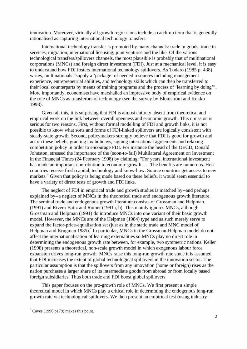
Preferences of the representative consumer (in both countries) are modelled as a Cobb-Douglas nest of Z consumption and a CES composite of X-varieties. Specifically:

5

U = C C , C c di , > 1Xt Zt1-

X

1

1-1/

i1-1/

i

N N

ln*

α ασ

σ σc h ≡FHG

IKJ=

+z0

(1)

where CZ and CX are Z-good consumption and the CES composite of manufactured goods (Nand N* are the number of home and foreign varieties resepectively), ci is consumption of X-variety i, and σ is the constant elasticity of substitution between any two varieties. Therepresentative consumer owns all the nation's L and K, so her income equals wL pluspayments to capital, πK; w and π are rewards to L and K (K's reward is the Ricardian surplusdue to variety-specificity).

2.2 Key Intermediate Results

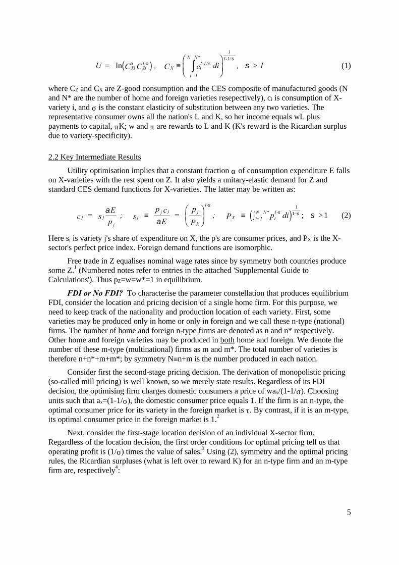
Utility optimisation implies that a constant fraction α of consumption expenditure E fallson X-varieties with the rest spent on Z. It also yields a unitary-elastic demand for Z andstandard CES demand functions for X-varieties. The latter may be written as:

j j

j

jj j

1-

j

XX i=1

N Ni1-

c = sE

p ; s

p c

E =

p

P; P p di

αα

σσ

σ σ≡FHG

IKJ ≡ z >+ −* ;d i

1

1 1 (2)

Here sj is variety j's share of expenditure on X, the p's are consumer prices, and PX is the X-sector's perfect price index. Foreign demand functions are isomorphic.

Free trade in Z equalises nominal wage rates since by symmetry both countries producesome Z.1 (Numbered notes refer to entries in the attached 'Supplemental Guide toCalculations'). Thus pZ=w=w*=1 in equilibrium.

FDI or No FDI? To characterise the parameter constellation that produces equilibriumFDI, consider the location and pricing decision of a single home firm. For this purpose, weneed to keep track of the nationality and production location of each variety. First, somevarieties may be produced only in home or only in foreign and we call these n-type (national)firms. The number of home and foreign n-type firms are denoted as n and n* respectively.Other home and foreign varieties may be produced in both home and foreign. We denote thenumber of these m-type (multinational) firms as m and m*. The total number of varieties istherefore n+n*+m+m*; by symmetry N≡n+m is the number produced in each nation.

Consider first the second-stage pricing decision. The derivation of monopolistic pricing(so-called mill pricing) is well known, so we merely state results. Regardless of its FDIdecision, the optimising firm charges domestic consumers a price of wax/(1-1/σ). Choosingunits such that ax=(1-1/σ), the domestic consumer price equals 1. If the firm is an n-type, theoptimal consumer price for its variety in the foreign market is τ. By contrast, if it is an m-type,its optimal consumer price in the foreign market is 1.2

Next, consider the first-stage location decision of an individual X-sector firm.Regardless of the location decision, the first order conditions for optimal pricing tell us thatoperating profit is (1/σ) times the value of sales.3 Using (2), symmetry and the optimal pricingrules, the Ricardian surpluses (what is left over to reward K) for an n-type firm and an m-typefirm are, respectively4:

6

n

m m

m

m mm=

1+ E N

2s + (1 - s )(1+ ), =

2 E N

2s + (1- s )(1+ )s

mN

N n mπφ α σ

φπ

α σφ

φ τ σ( )( / ) ( / ); , ,≡ ≡ + ≡ −1 (3)

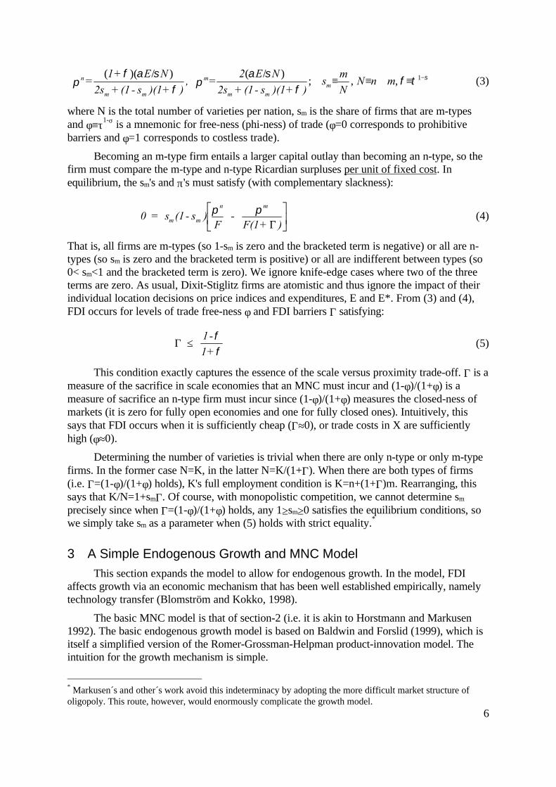
where N is the total number of varieties per nation, sm is the share of firms that are m-typesand φ≡τ1-σ is a mnemonic for free-ness (phi-ness) of trade (φ=0 corresponds to prohibitivebarriers and φ=1 corresponds to costless trade).

Becoming an m-type firm entails a larger capital outlay than becoming an n-type, so thefirm must compare the m-type and n-type Ricardian surpluses per unit of fixed cost. Inequilibrium, the sm's and π's must satisfy (with complementary slackness):

0 = s (1- s )F

- F(1+ )m m

n mπ πΓ

LNM

OQP (4)

That is, all firms are m-types (so 1-sm is zero and the bracketed term is negative) or all are n-types (so sm is zero and the bracketed term is positive) or all are indifferent between types (so0< sm<1 and the bracketed term is zero). We ignore knife-edge cases where two of the threeterms are zero. As usual, Dixit-Stiglitz firms are atomistic and thus ignore the impact of theirindividual location decisions on price indices and expenditures, E and E*. From (3) and (4),FDI occurs for levels of trade free-ness φ and FDI barriers Γ satisfying:

Γ 1-1+

≤φφ

(5)

This condition exactly captures the essence of the scale versus proximity trade-off. Γ is ameasure of the sacrifice in scale economies that an MNC must incur and (1-φ)/(1+φ) is ameasure of sacrifice an n-type firm must incur since (1-φ)/(1+φ) measures the closed-ness ofmarkets (it is zero for fully open economies and one for fully closed ones). Intuitively, thissays that FDI occurs when it is sufficiently cheap (Γ≈0), or trade costs in X are sufficientlyhigh (φ≈0).

Determining the number of varieties is trivial when there are only n-type or only m-typefirms. In the former case N=K, in the latter N=K/(1+Γ). When there are both types of firms(i.e. Γ=(1-φ)/(1+φ) holds), K's full employment condition is K=n+(1+Γ)m. Rearranging, thissays that K/N=1+smΓ. Of course, with monopolistic competition, we cannot determine sm

precisely since when Γ=(1-φ)/(1+φ) holds, any 1≥sm≥0 satisfies the equilibrium conditions, sowe simply take sm as a parameter when (5) holds with strict equality.*

3 A Simple Endogenous Growth and MNC Model

This section expands the model to allow for endogenous growth. In the model, FDIaffects growth via an economic mechanism that has been well established empirically, namelytechnology transfer (Blomström and Kokko, 1998).

The basic MNC model is that of section-2 (i.e. it is akin to Horstmann and Markusen1992). The basic endogenous growth model is based on Baldwin and Forslid (1999), which isitself a simplified version of the Romer-Grossman-Helpman product-innovation model. Theintuition for the growth mechanism is simple.

* Markusen´s and other´s work avoid this indeterminacy by adopting the more difficult market structure ofoligopoly. This route, however, would enormously complicate the growth model.

7

Long-run growth is always and everywhere based on the ceaseless accumulation ofcapital, typically human, physical or knowledge capital.* A central challenge faced byendogenous growth models is to explain how accumulation remains profitable in spite of theever-growing capital stock. For the Romer-Grossman-Helpman model, where each Dixit-Stiglitz variety is associated with a unit of capital, the specific question is how to keep thenumber of varieties continually growing despite the implied drop in operating profits. Thesolution is to find a way to keep the fixed cost F falling at a constant rate. The path-breakingassumption that justified this was introduced by Lucas (1988) and Romer (1990). Theypostulate a learning curve in the capital-producing sector.† That is, the labour required tomake a new unit of knowledge (equal to aI in our model) falls as the cumulative output of thecapital-producing sector rises. Combining the Lucas-Romer learning curve assumption withthe Krugman-Dixit-Norman trade model easily yields an elegant and tractable trade-and-endogenous-growth model, as Grossman and Helpman (1991) showed.

Since learning externalities in the capital producing (i.e. innovation) sector are at theheart of our endogenous growth model--and, as we shall see, at the heart of MNCs' growthimplications--a discussion of these externalities is in order.

3.1 Spillovers: the Engine of Tech-Transfer and Growth

Glaeser, Kallal, Scheinkman and Shleifer (1992) distinguish three types of dynamicexternalities (spillovers). The first two--the Marshall-Arrow-Romer (MAR) type and thePorter type--stem from ongoing communication among firms within a sector. For our model,differences between MAR and Porter externalities are moot and Romer applied them toendogenous growth, so we call them MAR or Romerian externalities. In many formulations ofMAR spillovers, the degree of spillovers is determined by location, rather than, say, the levelof economic intercourse among firms. The actual spillover mechanism envisaged in theseformulations can be via face-to-face discussions, telecommunications, scientific papers, orinformal exchange of workers via hires and fires. In any case, the basic idea is that knowledgeflows from one firm to another via a process that we can label "osmosis". Our model belowassumes a sector-wide learning curve in the knowledge-capital producing sector (i.e. theinnovation sector) where learning is of this "osmosis" or MAR type. Specifically, theproductivity of innovation-sector labour improves as the cumulative output, and thus theexperience level, of the innovation-sector rises. Variety-developers therefore get more efficientat developing varieties as more varieties are developed.‡

The third type of spillovers discussed by Glaeser, Kallal, Scheinkman and Shleifer(1992) is called Jacobian spillovers, after Jacobs (1969). These stem from a build up ofknowledge or ideas associated with diversity. Jacobian spillovers therefore involve learningacross sectors. In the Jacobian spillover approach, firms learn from other sectors and activities.Applying this to our model, we assume that X-sector manufacturing is a source of cost-saving

* In models such as the Solow and Young models, the accumulation is unintentional or exogenous.† Lucas, Romer and their followers describe this as a technological externality or 'knowledge spillovers', buttrade economists will recognise it as a learning curve. Lucas works with human capital and Romer withknowledge capital, but the logic is the same.‡ Grossman and Helpman (1991) justify the learning curve as follows. Developing a new variety produces twotypes of knowledge. The first type, which is appropriable, allows a new X-sector firm to produce a new variety.The second type is non-appropriable public knowledge that 'spills over' into the innovation-sector itself, thuslowering the marginal cost of developing further varieties. Innovation activity is both the source andbeneficiary of this spillover, so this is a within-sector (MAR) spillover.

8

spillovers to the I-sector. The idea here is that variety-developers in the innovation-sector cando their job more efficiently when able to observe a wide-range of X-sector manufacturingprocesses. This is a natural assumption in the present context since the full one-time costs ofdeveloping a new good must include development of a manufacturing process as well as itsdesign characteristics. To the extent that differentiated products are made with similar but notidentical production processes, developing manufacturing know-how may be easier whendevelopers can observe on-going manufacturing of existing varieties.

There is substantial empirical evidence that spillovers are partially localised (see Eatonand Kortum 1996, Cabellero and Jaffee 1993, and Keller 1997). That is, home innovatorslearn more from home-based innovation and manufacturing than they do from that which isdone abroad. We incorporate this into our model by assuming the beneficial effects of the"osmosis" are greater when innovators are in the same nation, while Jacobian spillovers onlyoperate within a country.

3.2 Introducing Endogenous Growth

The first additional assumption concerns intertemporal preferences. The instantaneouspreferences of the representative consumer (in both countries) are as in (1). The intertemporaldimension of preferences is made as simple as possible by assuming:

U = e C C dt , C c di , > 1s

t=s

- t sX Z

1-X

1

1-1/i=0N +N

i1-1/

*∞

−z ≡ zρ α α σσ σ( ) lnc h e j (6)

where ρ>0 is the rate of pure time preference. As is well known, utility optimisation impliesthe demand functions as in section 2, an Euler equation & /E E r= −ρ (r is the rate of return tosavings) and a transversality condition.6

The second extra assumption concerns the innovation sector (I-sector for short). The I-sector produces a new unit of K using aI units of L, where aI is subject to learning that isexternal to individual I-firms. All of the spillovers-considerations discussed above aretranscribed into the model via the I-sector learning curve. Formally, the learning curve is:

a = 1

K + K n+ m m ; 0 1 , 0I ( *) ( *)λ µ

λ µ+ +

≤ ≤ ≤ (7)

where λ measures the internationalisation of MAR spillovers and µ measures the importanceof Jacobian spillovers relative to MAR spillovers. In (7), K+λK* captures MAR spillovers thatoccur by "osmosis", i.e. are unrelated to the level of international commerce. The termn+m+m* reflects the Jacobian learning stemming from manufacturing undertaken by home-based firms (recall that m-type firms produce in both nations, so n+m+m* varieties areproduced in home). When λ=1, MAR spillovers are equally strong for all varieties regardlessof where they are invented. When λ is less than unity, spillovers are at least partially localised.

The implied I-sector production function gives the flow of new capital, QK, as:

Q K L aK I I≡ =& / (8)

Converting (8) to growth-rate form, using (7) and K=n+m(1+Γ), we get7:

9

g L A As

sIm

m

= ≡ + ++

+; 1

1

1λ µ

Γ(9)

where A is a measure of I-sector labour productivity that depends on spilloversparameters and the degree of multinationality, sm. Note that I-sector labour productivity isincreasing in the degree of multinationality. The expression for foreign is symmetric.

I-sector firms face perfect competition, so the price of capital is waI.*

Jones' Critique. The learning curve assumed above is standard in the trade-and-endogenous-growth literature, and as such displays so-called scale effects. Jones (1995) castsdoubt on the existence of scale effects, so some defence of our assumption is called for.

In the literature, the term scale-effect is applied to two distinct propositions. It is used todescribe the result, found in the earliest endogenous growth models, that bigger autarkicnations grow faster. This result, which is obviously rejected by the data, is not a seriousconsideration. The point is that endogenous-growth models that allow for any positive level ofinternational knowledge spillovers (e.g. Grossman and Helpman 1991) imply convergence oflong-run growth rates. Thus, apart from transitional effects, learning curves such as ours implythat all nations should grow at the same pace, in the long run. Obviously, nations do grow atdifferent rates, however it is plausible to view as transitory the high growth rates experiencedby particular nations.

The second, more serious use of the scale-effect terminology, focuses on the fact thatknowledge-production functions, such as (9), assume a unitary learning-elasticity (e.g. a 1%increase in K reduces F by 1%). This implies that output--i.e. the rate of technical progress--should be positively related to the level of inputs.** Jones (1995), which ignores internationalfactors and works with macro data, tests this by taking the number of R&D scientists andengineers as a proxy for inputs and total factor productivity (TFP) as a proxy for the output.He rejects the unitary learning elasticity since "TFP growth exhibits little or no persistentincrease, and even has a negative trend for some countries, while the measures of LA [Jones'notation for our LI] exhibit strong exponential growth."

Jones' claim, however, is no better than his proxy and TFP is a notoriously bad measureof innovation (Nelson 1996). In particular, TFP figures depend critically on aggregate priceindices that systematically underestimate the impact of quality and variety. This is a criticalshortcoming since mainstream endogenous growth models rely entirely on quality and/orvariety effects as their growth engines. Quite simply, a price index that is not revised everyyear to reflect expanding variety will systematically understate the TFP growth predicted bythe Romer-Grossman-Helpman product innovation model. To take an extreme example,suppose that TFP is measured with a price index that aggregates all varieties together (i.e. itdivides expenditure by the average price of varieties). Since the physical output of themanufacturing sector (X) is constant through time in the Grossman-Helpman model, such aprice index would indicate, as Jones found, that there was no relationship between LI and TFPgrowth--even if (9) were correct. The same problem holds a fortiori for quality-ladder models.Empirical price indices, after all, are famously unable to reflect quality improvements. Theseshortcomings have been addressed for goods such as computers, but not for services--whichaccount for about two-thirds of economic activity in OECD nations. * Imperfect competition in the I-sector permits consideration of new trade-growth links, but does not alter thefundamentally nature of steady-state growth (Baldwin and Forslid 1999).**In a closed economy & /K K L KI= −1 η ; if the learning elasticity η<1, LI must rise to keep & /K K constant.

10

Furthermore, Backus, Kehoe and Kehoe (1992) find evidence of scale effects inindustry-level data, as do we below. The fact that scale effects are found in industry data butnot in macro data (where services are dominant) lends further credence that Jones' result isbased on a mis-measurement of output, i.e. technological progress.

Jones (1995) raised important questions, but a sober evaluation of the evidence suggeststhat one cannot reject (9) until more detailed empirical work is undertaken. In any case, non-scale growth models do not provide substantially different implications concerning trade andgrowth links (e.g. Young 1998, or Baldwin and Seghezza 1996) and they are more complex towork with since they have transitional dynamics.

3.3 The Long-Run Dynamic Equilibrium

The simplest way to analyse the model, is to take L as numeraire (as assumed above)and to take LI as the state variable (i.e. the variable whose motion must stop in steady state).8

The simplest solution technique involves Tobin's q. LI is the amount of labour devoted to thecreation of new K, so it is, in essence, the national level of real investment. While there may bemany ways of determining investment in a general equilibrium model, Tobin's q-approach--introduced by Tobin (1969)--is a powerful, intuitive, and well-known method for doing justthat. The essence of Tobin's approach is to assert that the equilibrium level of investment ischaracterised by equality of the stock market value of a unit of capital--which we denote withthe symbol V--and the cost of capital, F. Tobin took the ratio of these, so what tradeeconomists would naturally call the X-sector free-entry condition becomes Tobin's famouscondition q≡V/F=1.

FDI or No FDI? The pricing and location decisions facing a typical firm in thisdynamic model are analogous to those in the static section-2 model. The pricing decision, inparticular, is identical since prices can be set independently in each period. The locationdecision is only slightly more complicated. If the firm becomes an n-type, the flow of operatingprofit (measured in units of L) is given by the first expression in (3); if it becomes an m-type,its operating profit flow is given by the second expression in (3).** The firm makes its decisionby comparing the present value of the two operating profit streams--call these Vn for n-typesand Vm for m-types--with the respective one-time costs, namely F and F(1+Γ).

Calculation of the steady-state V's is simple. It is intuitively obvious (and simple todemonstrate) that the steady-state discount rate is the rate of pure time preference ρ.9 Also, insteady state LI must be time-invariant (by definition of a state variable) and sm is time-invariant(it is zero, unity or an exogenous sm). Thus, from (9) and symmetry, K will grow at a time-invariant rate. From (3) and the time-invariance of nominal E, both πN and πM fall at the rate g.Of course, a flow that falls at g and is discounted at r=ρ has a present value of10:

V = + g

; i = n,miiπ

ρ(10)

X-sector firms are atomistic, so each firm takes as given the value of equilibriumvariables, such as g, when making their FDI decision. A new X-firm will, therefore, find itoptimal to set up a factory in both nations when πm/[(ρ+g)F(1+Γ)]≥πn/[(ρ+g)F]. Since 1/(ρ+g)enters both sides of the inequality, we see that the necessary and sufficient condition for FDI inthe dynamic model is identical to (5) from the static model, i.e. Γ≤( ) / ( )1- 1+φ φ . When this

**In the static model E is income; here it is income less investment.

11

condition holds with equality, the equilibrium sm is indeterminate as in section 2, so we take itas determined by factors outside of the model. A parsimonious summary is that:

0 = s (1- s ) VF

- VF(1+ )

; s mKm m

n m

mΓFHG

IKJ ≡ (11)

That is, all firms are m-types, all firms are n-types, or firms are indifferent between types. Notethat Vn/F and Vm/F[1+Γ] are the Tobin q's for n-type and m-type firms.

Equilibrium Growth. Consider the case where there are some MNCs, so the long-runaccumulation rate is determined by solving qm=qn=1. To find the steady-state flow of πm andthus the numerator of qm, Vm, we need expenditure. E is income less investment/savings, soE=L+πK-LI. With mark-up pricing and symmetry, total operating profit worldwide is α2E/σ.Half of this accrues to home residents, so E=(L-LI)/(1-α/σ). Using (3), (9) and the facts thatK/N=(1+smΓ) and Γ=(1-φ)/(1+φ) when 0<sm<1, steady state qm is11:

q =L L A

L Am I

I

ασ α ρ

( )

( )( )

−− +

(12)

Solving qm=1 for the steady-state LI and plugging the result into (9), we have:

g = LA - ( - )α ρ σ α

α σ1− +(13)

The expression for the no-FDI case and the all-FDI case, i.e. Γ>(1-φ)/(1+φ) and Γ<(1-φ)/(1+φ), is identical with sm=0 and sm=1 respectively.

The g's derived so far give the rate of knowledge capital accumulation, i.e. the rate atwhich new varieties are introduced. We turn now to real income growth. Nominal income,L+πiK (i=N, M), is time-invariant along any steady state growth path (π and K grow atopposite rates). Real income growth is thus the opposite of the rate of decline of the perfectprice index. Given the usual CES perfect price index and (13):

GDPg = g- 1

ασ

(14)

The growth rate with no MNCs is given by (13) and (14) with sm=0.

The equilibrium growth rate rises with the degree of multinationality sm. To see this,note that gGDP is monotonically increasing in g, and g is monotonically increasing in sm since Arises with sm. Intuitively this should be obvious. sm has no impact on π, yet it raises theproductivity of I-sector workers and thus lowers the cost of innovation. In other words,raising sm, leads to an incipient rise in Tobin's q since it lowers the replacement cost ofknowledge capital. As Baldwin and Forslid (1999) Proposition 1 shows, anything that leads toan incipient rise in q is pro-growth.

4 Empirical Analysis

We turn now to the evidence, first deriving our main estimating equations beforediscussing data issues and presenting our results.

12

4.1 The Estimating Equation

Our empirical work focuses on labour-productivity growth in manufacturing sectors, sothe first task is to find the equilibrium expression for this from the Section 3 model.

Value added and output are identical in our theoretical model because intermediateinputs are assumed away. Value added in the industrial X-sector is, therefore, the equilibriumnominal output divided by the sector’s perfect price index PX. Since varieties are symmetric,the value of output equals the producer price times the labour input (LX) divided by the unit-input coefficient (ax≡1-1/σ). The producer price is unity (due to mark-up pricing and ourchoice of units and numeraire), so real output is LX/(1-1/σ) divided by (PX)α. Using thedefinition of PX from (2), labour productivity (value added per worker) is:

y p diX ii

N N=

−FH IK−

=

+ −z1

1 11

0

1

/

*

σσ

ασ

(15)

where yX is real value-added per worker.

Nominal output is time-invariant in steady state. X-sector labour productivity (yX) thusgrows at the rate that (PX)α falls. In steady state, this rate is α/(σ-1) times g, so from (9) thegrowth of yX is:

& *y

yL

KK

Ls

sLX

XI I

m

mI=

−+ +

++

FHG

IKJ

ασ

λ µ1

1

1 Γ(16)

Our estimations are based on this equation.

4.2 Data and Construction of Variables

Our data cover a cross section of seven manufacturing industries in nine OECD-countries. The industries comprise processed food, textiles and clothing, paper, chemicals,non-metallic mineral products, basic metal industries, and machinery and equipment (i.e. ISICgroups 31, 32, 34, 35, 36, 37 and 38). The list of countries is Canada, Denmark, France,

Germany, Italy, Japan, Sweden, the UK and the US.

Data were collected from a number of sources. Data on value added, employment,capital stocks, exports and imports are from ISDB (1994). R&D-expenditures are taken from

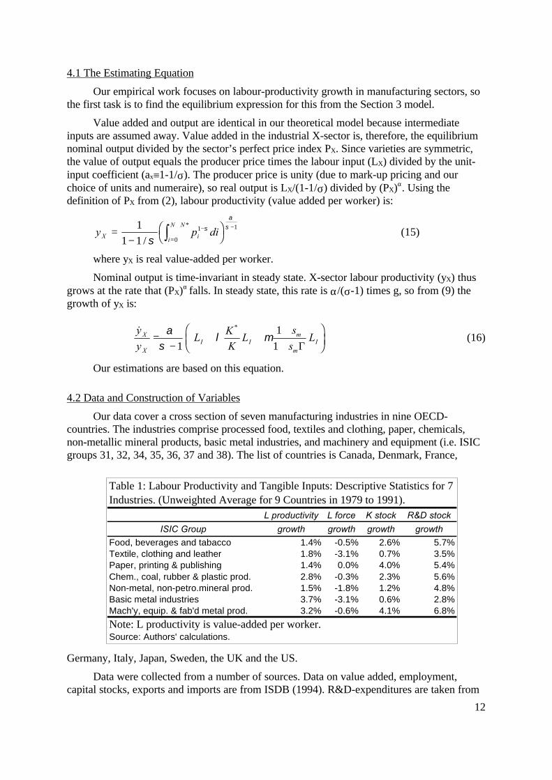
Table 1: Labour Productivity and Tangible Inputs: Descriptive Statistics for 7 Industries. (Unweighted Average for 9 Countries in 1979 to 1991).

L productivity L force K stock R&D stock

ISIC Group growth growth growth growth

Food, beverages and tabacco 1.4% -0.5% 2.6% 5.7%Textile, clothing and leather 1.8% -3.1% 0.7% 3.5%Paper, printing & publishing 1.4% 0.0% 4.0% 5.4%Chem., coal, rubber & plastic prod. 2.8% -0.3% 2.3% 5.6%Non-metal, non-petro.mineral prod. 1.5% -1.8% 1.2% 4.8%Basic metal industries 3.7% -3.1% 0.6% 2.8%Mach'y, equip. & fab'd metal prod. 3.2% -0.6% 4.1% 6.8%

Note: L productivity is value-added per worker.Source: Authors' calculations.

13

ANBERD (1994), Science, and Technology Indicators: Basic Statistical Series-Volume D(1983), while PPP-estimates and GDP-deflators are from the OECD Economic Outlook(various issues). Finally, stocks of foreign direct investment (FDI) have been computed fromdata from the World Investment Directory (1993) published by the UN.* Stocks of knowledgeare computed (according to the perpetual inventory method) using real R&D spending in eachsector from 1963 and onwards.† Reported results are based on an assumed rate of depreciationequal to 5 percent. All variables are in 1990 US $ equivalents and based on average values forthe period 1979-1991.

Table 1 shows summary statistics on the sectors’ labour productivity growth (i.e.growth in value-added per employee) and the input growth (un-weighted averages for the ninecountries). The first column gives labour-productivity growth performance by sector and herewe see a good deal of variation. At the high end, labour productivity in the basic metal

industries grew 3.7% on average, while at the low end, the food, beverages and tobaccosector and the paper sector grew at only 1.4%. The next three columns present figures for thegrowth of inputs. Employment in all sectors fell, but physical and knowledge capital inputsrose.

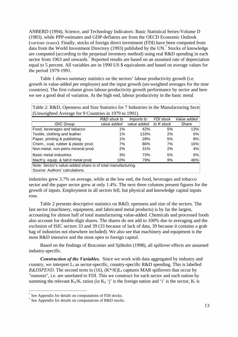
Table 2 presents descriptive statistics on R&D, openness and size of the sectors. Thelast sector (machinery, equipment, and fabricated metal products) is by far the largest,accounting for almost half of total manufacturing value-added. Chemicals and processed foodsalso account for double-digit shares. The shares do not add to 100% due to averaging and theexclusion of ISIC sectors 33 and 39 (33 because of lack of data, 39 because it contains a grabbag of industries not elsewhere included). We also see that machinery and equipment is themost R&D intensive and the most open to foreign capital.

Based on the findings of Braconier and Sjöholm (1998), all spillover effects are assumedindustry-specific.

Construction of the Variables. Since we work with data aggregated by industry andcountry, we interpret LI as sector-specific, country-specific R&D spending. This is labelledR&DSPEND. The second term in (16), (K*/K)LI captures MAR spillovers that occur by"osmosis", i.e. are unrelated to FDI. This we construct for each sector and each nation bysumming the relevant Kij/Ki ratios (in Kij ‘j’ is the foreign nation and ‘i’ is the sector, Ki is

* See Appendix for details on computations of FDI stocks.† See Appendix for details on computations of R&D stocks.

Table 2: R&D, Openness and Size Statistics for 7 Industries in the Manufacturing Sector (Unweighted Average for 9 Countries in 1979 to 1991).

R&D stock to Imports to FDI stock Value addedISIC Group value added value added to K stock Share

Food, beverages and tabacco 1% 42% 5% 13%Textile, clothing and leather 1% 133% 2% 6%Paper, printing & publishing 1% 28% 5% 8%Chem., coal, rubber & plastic prod. 7% 86% 7% 16%Non-metal, non-petro.mineral prod. 2% 31% 2% 4%

Basic metal industries 3% 73% 5% 6%Mach'y, equip. & fab'd metal prod. 10% 79% 9% 46%Note: Sector's value-added share is of total manufacturing.Source: Authors' calculations.

14

home-nation's K in sector i; the K’s are our calculated R&D capital stocks). We call thisconstructed variable, MAR-SPILL (short for Marshall-Arrow-Romer spillovers).

The third term captures FDI-linked spillovers. Our theoretical model provides only arough guide to constructing this variable since K is both the stock of local experience in theR&D sector, and proportional to the number of local firms. Moreover, the model has only asingle industry but empirically we must account for cross-sector diversity in R&D intensityleading to different degrees of FDI-linked spillovers. A foreign-owned bottling plant, forinstance, is likely to provide fewer spillovers than a foreign-owned pharmaceutical plant. Toallow for this we construct a variable that reflects the R&D intensity of each sector in eachFDI source-country. Specifically, for each partner country j, we multiply two ratios. The firstratio reflects R&D intensity by sector and source country. It is (Kij/Mij), where Kij is the j'sknowledge stock in industry i and Mij is j's physical capital stock (M is a mnemonic formachines) in industry i. The second ratio reflects importance of each source country. It isFDIij/Mi where FDIij is the inward FDI flow from j in sector i and Mi is the home nation'sphysical capital stock in sector i. The products of the pair of ratios for each partner countryare summed and the result is multiplied by LI, i.e. the flow of home-country R&D spending insector i. The variable is called FDI-SPILL.

4.3 Econometric Results

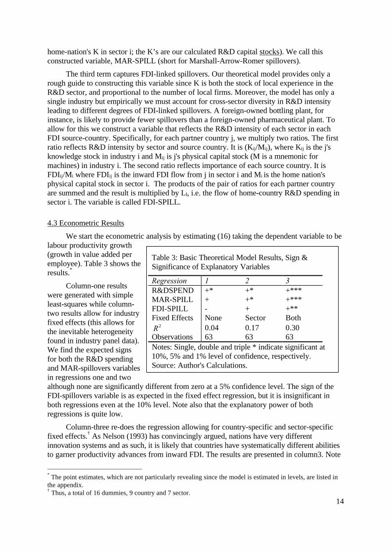
We start the econometric analysis by estimating (16) taking the dependent variable to belabour productivity growth(growth in value added peremployee). Table 3 shows theresults.*

Column-one resultswere generated with simpleleast-squares while column-two results allow for industryfixed effects (this allows forthe inevitable heterogeneityfound in industry panel data).We find the expected signsfor both the R&D spendingand MAR-spillovers variablesin regressions one and twoalthough none are significantly different from zero at a 5% confidence level. The sign of theFDI-spillovers variable is as expected in the fixed effect regression, but it is insignificant inboth regressions even at the 10% level. Note also that the explanatory power of bothregressions is quite low.

Column-three re-does the regression allowing for country-specific and sector-specificfixed effects.† As Nelson (1993) has convincingly argued, nations have very differentinnovation systems and as such, it is likely that countries have systematically different abilitiesto garner productivity advances from inward FDI. The results are presented in column3. Note

* The point estimates, which are not particularly revealing since the model is estimated in levels, are listed inthe appendix.† Thus, a total of 16 dummies, 9 country and 7 sector.

Table 3: Basic Theoretical Model Results, Sign &Significance of Explanatory Variables

Regression 1 2 3R&DSPEND +* +* +***MAR-SPILL + +* +***FDI-SPILL - + +**Fixed Effects None Sector BothR2 0.04 0.17 0.30Observations 63 63 63Notes: Single, double and triple * indicate significant at10%, 5% and 1% level of confidence, respectively.Source: Author's Calculations.

15

first that the explanatory power rises and although the signs do not change compared tocolumn-2, the coefficients all become significant.

Overall, Table 3 provides a modicum of support for the basic model. The maininnovation variables have the expected sign. In particular, we find strong evidence of the"osmosis" type spillovers. We also find evidence that FDI leads to knowledge spilloversbeyond the "osmosis" type. In this sense, we can say that FDI appears to promote growth bypromoting technology transfer. Interestingly, the significant and positive sign on LI confirmsthe findings ofBackus, Kehoe andKehoe (1992) that so-called scale effects doexist in industry leveldata.

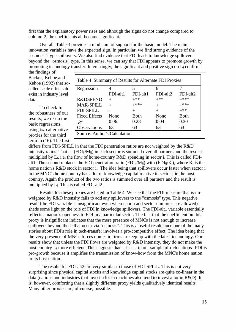
To check forthe robustness of ourresults, we re-do thebasic regressionsusing two alternativeproxies for the thirdterm in (16). The firstdiffers from FDI-SPILL in that the FDI penetration ratios are not weighted by the R&Dintensity ratios. That is, (FDIij/Mij) in each sector is summed over all partners and the result ismultiplied by LI, i.e. the flow of home-country R&D spending in sector i. This is called FDI-alt1. The second replaces the FDI penetration ratio (FDIij/Mij) with (FDIij/Ki), where Ki is thehome nation's R&D stock in sector i. The idea being that spillovers occur faster when sector iin the MNC's home country has a lot of knowledge capital relative to sector i in the hostcountry. Again the product of the two ratios is summed over all partners and the result ismultiplied by LI. This is called FDI-alt2.

Results for these proxies are listed in Table 4. We see that the FDI measure that is un-weighted by R&D intensity fails to add any spillovers to the "osmosis" type. This negativeresult (the FDI variable is insignificant even when nation and sector dummies are allowed)sheds some light on the role of FDI in knowledge spillovers. The FDI-alt1 variable essentiallyreflects a nation's openness to FDI in a particular sector. The fact that the coefficient on thisproxy is insignificant indicates that the mere presence of MNCs is not enough to increasespillovers beyond those that occur via "osmosis". This is a useful result since one of the manystories about FDI's role in tech-transfer involves a pro-competitive effect. The idea being thatthe very presence of MNCs forces domestic firms to keep up with the latest technology. Ourresults show that unless the FDI flows are weighted by R&D intensity, they do not make thehost country LI more efficient. This suggests that--at least in our sample of rich nations--FDI ispro-growth because it amplifies the transmission of know-how from the MNC's home nationto its host nation.

The results for FDI-alt2 are very similar to those of FDI-SPILL. This is not verysurprising since physical capital stocks and knowledge capital stocks are quite co-linear in thedata (nations and industries that invest a lot in machines also tend to invest a lot in R&D). Itis, however, comforting that a slightly different proxy yields qualitatively identical results.Many other proxies are, of course, possible.

Table 4 Summary of Results for Alternate FDI Proxies

Regression 4FDI-alt1

5FDI-alt1

6FDI-alt2

7FDI-alt2

R&DSPEND + +** +** +***MAR-SPILL + +*** + +***FDI-SPILL - + + +**Fixed Effects None Both None BothR2 0.06 0.28 0.04 0.30Observations 63 63 63 63Source: Author's Calculations.

16

5 Conclusions

FDI is almost entirely absent from theoretical and empirical work on the overall linkbetween openness and growth, despite the mass of empirical and anecdotal evidence showingMNCs to be important transferors of technology. This is a serious shortcoming, given thestrongly held belief that FDI is good for growth.

The neglect of FDI in empirical trade and growth studies is matched by - but alsoexplained by - a neglect of MNCs in the theoretical trade and endogenous growth literature.The seminal trade and endogenous growth literature - Grossman and Helpman (1991) andRivera-Batiz and Romer (1991a, b) - mainly ignores MNCs. Grossman and Helpman (1991)do introduce MNCs into one variant of their basic growth model. However, MNCs in thismodel are of the Helpman (1984) type and as such merely serve to expand the factor-priceequalisation set in a manner analogous to the static trade and MNC model in Helpman andKrugman (1985). In particular, MNCs in the Grossman-Helpman model do not affect theinternationalisation of learning externalities, so MNCs play no direct role in determining theendogenous growth rate.

This paper focuses on the pro-growth role of MNCs. We first present a simpletheoretical model in which MNCs play a critical role in determining the endogenous long-rungrowth rate via technological spillovers. We then present an empirical test (using industry-level panel data from seven OECD nations) that broadly supports our model.

Our findings are far from conclusive, but they do suggest that more theoretical andempirical work needs to be done on the growth effects of MNCs.

17

ReferencesBackus, D., Kehoe, P. and T. Kehoe, 1992, In Search of Scale Effects in Trade and Growth,

Journal of Economic Theory 58, 377-409.

Baldwin and Seghezza, 1996, Trade induced investment-led growth, NBER WP 5582.

Baldwin R. E. and R. Forslid, 1999, Trade Liberalisation and Endogenous Growth, Journal ofInternational Economics, forthcoming; also NBER WP 5549, 1997.

Barro, R., 1991, Economic Growth in a Cross-Section of Countries, Quarterly Journal ofEconomics 61, 407-443.

Blomström, M. and A. Kokko, 1998, Multinational corporations and spillovers, Journal ofEconomic Surveys 12, Also CEPR DP 1365.

Braconier, H. and F. Sjöholm, 1998, National and International Spillovers from R&D:Comparing a Neoclassical and an Endogenous Growth Approach, WeltwirtschaftlichesArchiv 134, 638-663.

Brainard, S.L., 1993, An empirical assessment of the proximity-concentration tradeoffbetween multinational sales and trade, NBER WP 4583.

Caballero, R. and A. Jaffe, 1993, How high are the ‘giants’ shoulders?, in O.Blanchard and S.Fischer, eds., NBER Macroeconomics Annual (NBER, Cambridge).

Carr, Markusen and Maskus, 1998, Estimating the Knowledge-Capital Model of theMultinational Enterprise, NBER WP 6773.

Caves, R.E., 1996, Multinational enterprise and economic analysis, Cambridge UniversityPress, Cambridge.

Coe, D. and E. Helpman, 1995, International R&D spillovers, European Economic Review39, 859-887.

Coe, D. and R. Moghadam, 1993, Capital and Trade as Engines of Growth in France, IMFStaff Papers 40, 542-566.

Dixit, A. and V. Norman, 1980, Theory of International Trade (Cambridge University Press,Cambridge).

Eaton, J. and S. Kortum, 1996, Trade in ideas: Productivity and patenting in the OECD,Journal of International Economics 40, 251-278.

Edwards, S., 1997, Openness, Productivity and Growth: What Do We Really Know?, NBERWP 5978.

Feenstra, R.C., 1996, Trade and uneven growth, Journal of Development Economics 49, 229-256.

Glaeser, E., H. Kallal, J. Scheinkman and A. Shleifer, 1992, Journal of Political Economy 100,1126-1153.

Globerman, S., 1979, Foreign direct investment and ‘spillover’ efficiency benefits in Canadianmanufacturing industries, Canadian Journal of Economics 7, 42-56.

Grossman, G. and E. Helpman, 1991, Innovation and Growth in the World Economy, (MITPress, Cambridge).

Grossman, G. and E. Helpman, 1995, Technology and Trade, in G. Grossman and K. Rogoff,

18

eds, Handbook of International Economics, Vol. 3 (North-Holland, Amsterdam) 1279-1338.

Harrison, A., 1996, Openness and growth: A time-series, cross-country analysis fordeveloping countries, Journal of Development Economics 48, 419-447.

Helpman, E. and P. Krugman, 1985, Market Structure and Foreign Trade, (MIT Press,Cambridge).

Helpman, E., 1994, A simple theory of international trade with multinational corporations,Journal of Political Economy 92, 451-471.

Horstmann, I. and J. Markusen, 1987, Strategic investments and the development ofmultinationals, International Economic Review 28, 109-121.

Horstmann, I. and J. Markusen, 1992, Endogenous market structure in international trade,Journal of International Economics 9, 169-189.

Hummels, D. and R. Stern, 1994, Evolving patterns of North American merchandise trade andforeign direct investment, 1960-1990, World Economy 17, 5-29.

Jacobs, J., 1969, The Economy of Cities, New York, Vintage.

Jones, C., 1995, Time series tests of endogenous growth models, Quarterly Journal ofEconomics 110, 495-527.

Keller, W., 1998, Multinational enterprises, international trade and technology diffusion,manuscript, August 1998.

Keller, W., 1997, Are international R&D spillovers trade-related? Analysing spillovers amongrandomly matched trade partners, NBER Working Paper 6065.

Krugman,P., 1980, Scale economies, product differentiation and the pattern of trade,American Economic Review 70, 950-959.

Krugman, P., 1988, Endogenous Innovation, International Trade and Growth, manuscript,reprinted in P. Krugman, 1990, Rethinking International Trade, (MIT Press,Cambridge).

Lucas, R., 1988, On the mechanics of economic development, Journal of MonetaryEconomics 22, 3-42.

Markusen, J., A. Venables, D. Konan and K. Zhang, 1998, A Unified Treatment of HorizontalDirect Investment, Vertical Direct Investment, and the Pattern of Trade in Goods andServices, NBER WP 5696.

Markusen, J., 1995, The boundaries of multinational enterprises and the theory of internationaltrade, Journal of Economic Perspectives 9, 169-189.

Nelson, R., 1993, National innovation systems: a comparative analysis (Oxford UniversityPress, NY).

Nelson, R., 1996, The sources of economic growth (Harvard University Press, Cambridge).

OECD, 1983, Science and Technology Indicators: Basic Statistical Series - Volume D.

OECD, 1992, Analytical Business Enterprise R&D (ANBERD).

OECD, 1994, Industrial Statistics Database (ISDB).

19

OECD, various issues, Economic Outlook.

Rivera-Batiz, L. and P. Romer, 1991a, Economic Integration and Endogenous Growth,Quarterly Journal of Economics 106, 531-555.

Rivera-Batiz, L. and P. Romer, 1991b, International Trade with Endogenous TechnologicalChange, European Economic Review 35, 715-721.

Romer, P., 1990, Endogenous Technological Change, Journal of Political Economy 98, 71-102.

Tobin, J., 1969, A General Equilibrium Approach to Monetary Theory, Journal of Money,Credit and Banking, 15-29.

Todaro, M., 1985, Economic development in the third world, Longman, London.

United Nations Transnational Corporations and Management Division, 1993, WorldInvestment Directory: Developed Countries, III.

Appendix

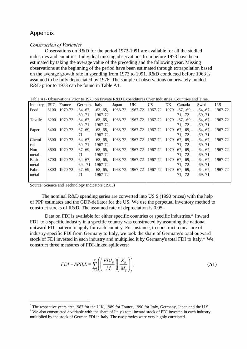
Construction of VariablesObservations on R&D for the period 1973-1991 are available for all the studied

industries and countries. Individual missing observations from before 1973 have beenestimated by taking the average value of the preceding and the following year. Missingobservations at the beginning of the period have been estimated through extrapolation basedon the average growth rate in spending from 1973 to 1991. R&D conducted before 1963 isassumed to be fully depreciated by 1978. The sample of observations on privately fundedR&D prior to 1973 can be found in Table A1.

Table A1- Observations Prior to 1973 on Private R&D Expenditures Over Industries, Countries and Time.Industry ISIC France German. Italy Japan UK US DK Canada Swed U.SFood

Textile

Paper

Chemi-calNon-metal.Basic-metalFabr.metal

3100

3200

3400

3500

3600

3700

3800

1970-72

1970-72

1970-72

1970-72

1970-72

1970-72

1970-72

-64,-67,-69,-71-64,-67,-69,-71-67,-69,-71-64,-67,-69,-71-67,-69,-71-64,-67,-69, -71-67,-69,-71

-63,-65,1967-72-63,-65,1967-72-63,-65,1967-72-63,-65,1967-72-63,-65,1967-72-63,-65,1967-72-63,-65,1967-72

1963-72

1963-72

1963-72

1963-72

1963-72

1963-72

1963-72

1967-72

1967-72

1967-72

1967-72

1967-72

1967-72

1967-72

1967-72

1967-72

1967-72

1967-72

1967-72

1967-72

1967-72

1970

1970

1970

1970

1970

1970

1970

-67, -69, -71, -72-67, -69, -71, -72 –67, -69, -71, -72 –67, -69, -71, -72 –67, -69, -71, -72 –67, -69, -71, -72 –67, -69, -71, -72

-64,-67,-69,-71-64,-67,-69,-71-64,-67,-69,-71-64,-67,-69,-71-64,-67,-69,-71-64,-67,-69,-71-64,-67,-69,-71

1967-72

1967-72

1967-72

1967-72

1967-72

1967-72

1967-72

Source: Science and Technology Indicators (1983)

The nominal R&D spending series are converted into US $ (1990 prices) with the helpof PPP estimates and the GDP-deflator for the US. We use the perpetual inventory method toconstruct stocks of R&D. The assumed rate of depreciation is 0.05.

Data on FDI is available for either specific countries or specific industries.* InwardFDI to a specific industry in a specific country was constructed by assuming the nationaloutward FDI-pattern to apply for each country. For instance, to construct a measure ofindustry-specific FDI from Germany to Italy, we took the share of Germany's total outwardstock of FDI invested in each industry and multiplied it by Germany's total FDI to Italy.† Weconstruct three measures of FDI-linked spillovers:

FDI SPILLFDI

M

K

Mij

i

ij

ijj

n

− =FHG

IKJFHG

IKJ

FHG

IKJ=

∑1,

, (A1)

* The respective years are: 1987 for the U.K, 1989 for France, 1990 for Italy, Germany, Japan and the U.S.† We also constructed a variable with the share of Italy's total inward stock of FDI invested in each industrymultiplied by the stock of German FDI in Italy. The two proxies were very highly correlated.

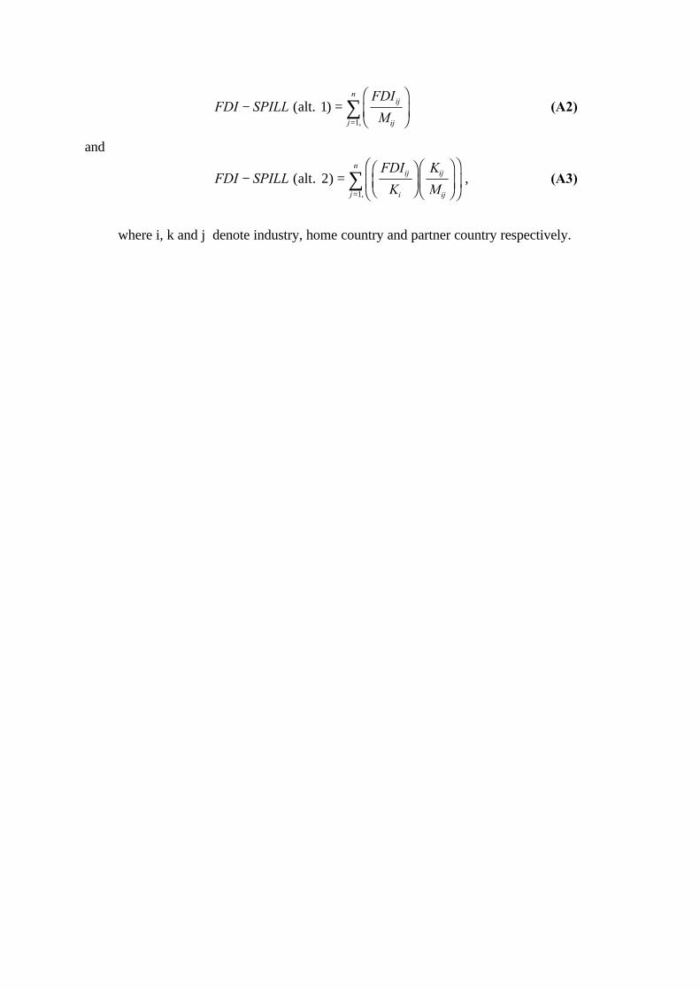
FDI SPILLFDI

Mij

ijj

n

− =FHG

IKJ=

∑ alt. 1( ),1

(A2)

and

FDI SPILLFDI

K

K

Mij

i

ij

ijj

n

− =FHG

IKJFHG

IKJ

FHG

IKJ=

∑ alt ( . ),

21

, (A3)

where i, k and j denote industry, home country and partner country respectively.

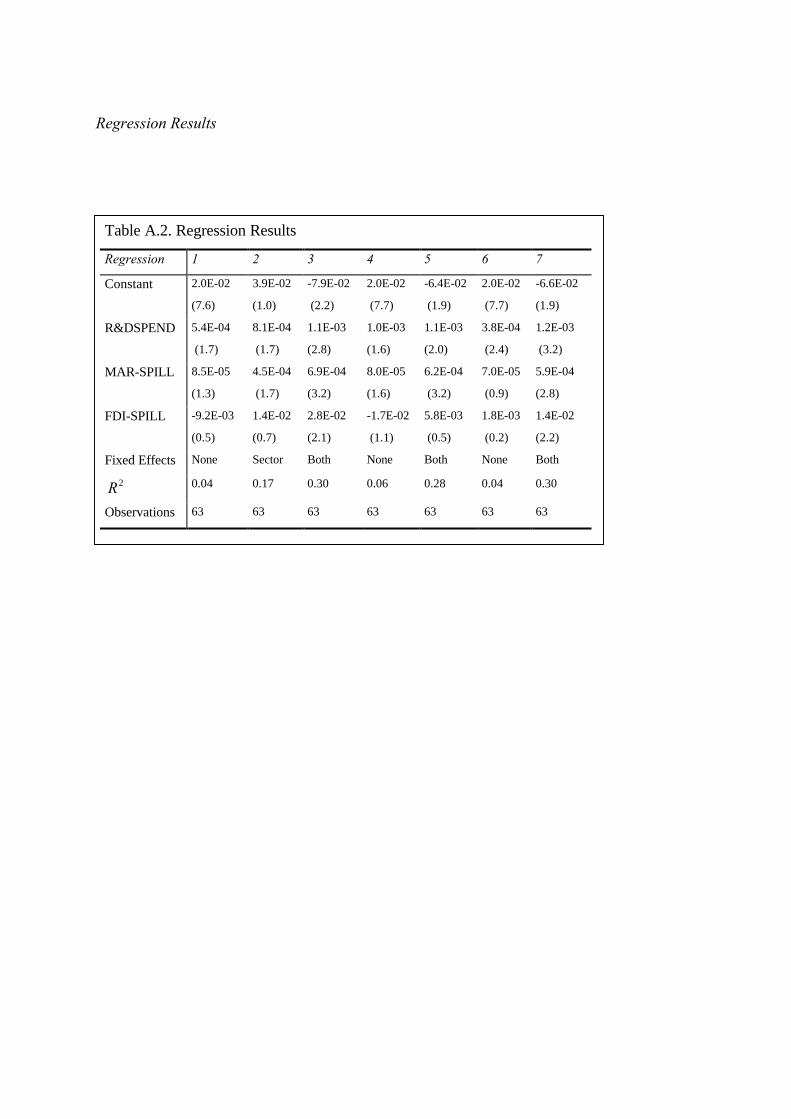
Regression Results

Table A.2. Regression Results

Regression 1 2 3 4 5 6 7

Constant 2.0E-02

(7.6)

3.9E-02

(1.0)

-7.9E-02

(2.2)

2.0E-02

(7.7)

-6.4E-02

(1.9)

2.0E-02

(7.7)

-6.6E-02

(1.9)

R&DSPEND 5.4E-04

(1.7)

8.1E-04

(1.7)

1.1E-03

(2.8)

1.0E-03

(1.6)

1.1E-03

(2.0)

3.8E-04

(2.4)

1.2E-03

(3.2)

MAR-SPILL 8.5E-05

(1.3)

4.5E-04

(1.7)

6.9E-04

(3.2)

8.0E-05

(1.6)

6.2E-04

(3.2)

7.0E-05

(0.9)

5.9E-04

(2.8)

FDI-SPILL -9.2E-03

(0.5)

1.4E-02

(0.7)

2.8E-02

(2.1)

-1.7E-02

(1.1)

5.8E-03

(0.5)

1.8E-03

(0.2)

1.4E-02

(2.2)

Fixed Effects None Sector Both None Both None Both

R2 0.04 0.17 0.30 0.06 0.28 0.04 0.30

Observations 63 63 63 63 63 63 63

SUPPLEMENTAL GUIDE TO CALCULATIONS

1. Without symmetry, a formal sufficient condition is that max{L, L*} is insufficient to meetglobal demand for Z. Since aZ=1 this requires that max{L, L*}<(1-α)Ew, where Ew is worldexpenditure. αEw is total spending on X and the monopolistic operating-profit margin is 1/σ,so Ew equals Lw plus αEw/σ. Rearranging, max{L, L*}<(1-α)σLw/(σ-α). This places limits onthe degree of size asymmetry that is consistent with factor price equalisation.2. All these prices follow from the fact that monopolistically competitive firms engage in 'millpricing', that ax=1-1/σ and w=w*=1.3. Consider the case of an n-type firm where operating profit earned on local sales is (p-ax)cand the operating profit earned on export sales is (p*-axτ)c*. The first order condition forlocal sales can be rearranged into (recall w=1):p(1-1 / ) = wa <=> (p - wa ) = p / <=> (p - wa )c = pc /x x xσ σ σ

where c is home consumption of the particular variety. Thus, the operating profit is 1/σ timessales. Similar manipulations show the same result for export sales. For m-type firms all salesare local.4. As always with monopolistic competition, operating profit is 1/σ times the value of sales(consumption at consumer prices or shipments at producer prices). The key to deriving theformula in the text is therefore to relate the value of sales to τ, n and m. Since locallyproduced varieties have a consumer price of 1 and nonlocally produced varieties a price of τ(due to optimal pricing), the CES demand function implies that the share of a locally producedvariety is:

s = n+ m+ m*+ n

; , NB: 0 1*

1-1

φφ τ φσ≡ ≤ ≤

since n+m+m* varieties are produced locally and n* varieties are imported. Using symmetryand defining θm as the share of a typical nation's firms that are m-types, s becomes:

s = 1

(1- s )(1+ )+ 2s

1K

; s m

n+ mm mmφ

≡

Likewise the share of an imported variety s* is:

*

m m

s = (1- s )(1+ )+ 2 s

1K

φφ

Similar manipulations yield the shares for an m-type firm (such firms have s in both markets).

6. Given that preferences are intertemporally separable and consumers take the path of pricesas given, we can solve the utility maximisation problem in two stages. The first is to determinethe optimal path of consumption expenditure E. To this end we set up the Hamiltonian, whichfor this problem is:

H[E,K, ,t] = e (EP

) + (K + wL - E

P)- t

K

λ λ πρ lnFHG

IKJ where C=E/P, P is the perfect price

index, PK is the price of K, and the law of motion for the representative consumer's wealth isK=(Y-E)/F since K is the only store of value. The four standard necessary conditions forintertemporal utility maximisation are:

∂∂

FHG

IKJ

∂∂

∞

HE

= 0 <=> e 1E

- P

= 0

d edt

= -HK

<=> - = P

law of motion <=> K = (Y - E) / F

transversality condition <=> li m (t)K(t) = 0

- t

K

- t

K

t ->

ρ

ρ

λ

λ ρ λλ

π

λ

&

&

The first three conditions characterise the optimum path at all moments in time, while thetransversality condition is only an endpoint condition. The total time derivative of the firstexpression can be used to eliminate λ from the second expression. The result reduces to:

& &EE

= (P

+ PP

) - K

K

K

π ρ

The Euler equation is found by noting that the right-hand expression in parentheses is the rateof return to K (the first term is the 'dividend' component and the second is the 'capital gains'component) and that this is the rate of return to savings, viz. r.

7 Grouping terms in (7), we have:

1 1/*

(*

)a KK

K

N

N

m

N

N

KI = + + +FHG

IKJλ µ

Since K=n+m(1+Γ), K/N=1+smΓ. Using this and symmetry yields:

1 11

1/ a K

s

sIm

m

= + ++

+FHG

IKJλ µ

ΓWith this, the expression in the text is easily obtained.

8 These are somewhat unconventional choices for numeraire and state variable, but theycan be justified as follows. First, consider why L is the natural numeraire. The model has onlyone primary factor, L, so expenditure allocation by the representative consumer is tantamountto resource allocation. When the consumer optimally decides to save a certain fraction of herincome, she is implicitly directing the same fractions of GDP to the production of investmentgoods. This is true regardless of numeraire, but it comes out most clearly with labour isnumeraire.

Consider next why LI is the natural state variable. The primary goal of any growth model is toidentify the endogenously determined growth rate. Most simple models--Romer (1986, 1990),Lucas (1988), Grossman and Helpman (1991) and the model in this paper--make assumptionsthat allow the steady-state growth rate to be constant. In all these models, the intersectoralallocation of primary resources is constant along the steady-state growth path. It is thereforenatural to focus on the time-invariant allocation of primary resources. After all, solving for theequilibrium allocation of labour among sectors is something that trade economists have beendoing for centuries. Baldwin and Forsild (1999) refer to this as the static-economyrepresentation of the steady-state growth path.

9.Since LI is the state variable, LI must, by definition, be time-invariant in steady state. Since alllabour is employed, this implies that the amount of labour employed in creating goods forconsumption is also time invariant. Given the X- and Z-sector production function, we knowthat the steady-state output of consumption goods--measured in terms of the numeraire L--must also is time invariant. Moreover the goods markets must clear, so consumer spending onthis time-invariant flow of goods must also be time invariant. We see directly, therefore,thatEQ &E = 0 in steady state, in both nations. From the Euler equations this implies thatEQ rEQ=r*=ρ.

More formally, E=Y-I, where I is spending on investment goods and Y=wL+mπM+nπN

is national income (i.e. income of the representative consumer). To prove the assertion, weneed to express E in terms of parameters and the state variable. This tells us that E stopsmoving in steady state since parameters and state variables do not evolve in steady state.

Since the I sector is competitive, I=wLI and by choice of numeraire w=1. π might seemmore involved since there may be α2E/σ. Half of this accrues to capital in each nation soE=L+αE/σ-LI, i.e. E =(L-LI)/(1-α/σ). Plainly this is time-invariant in steady state, soEQr=rEQ*=ρ in steady state.10. The present value of the πi stream, namely:

s=t-r(s-t)

si e ds∞z π Since g is time-invariant, Ks=Kte

gs in steady state. Thus π falls at the constant

rate EQg and:

t

s=t

-r(s-t)s t

s=t

-( +g)(s-t)J = e ds = e ds∞ ∞z zπ π ρ

Solution of the integral yields the formula in the text.

11 The denominator of q is waI(1+Γ) i.e.

( )( )

11

11

1

++

+Γ

Γ

Γ

a = 1K

+

+ s

+ s

Im

m

λ µ

where sm=m/N and w=1. The numerator is:

V =E

N g sm

m

ασ ρ φ φ( )

(( )

)+ − + +

2

1 1

since K =N(1+smΓ), Γ=(1-φ)/(1+φ) and (1+Γ )(1+φ)=2, this becomes:

V =E

g Km α

σ ρ( )( )

++1 Γ

The numerator and denominator together yield:

q =E A

gm α

σ ρ( )+Using E/σ=(L-LI)/(σ-α) and the growth rate form of the I-sector production function:

q =2 L L A

L Am I

I

ασ α ρ

( )

( )( )

−− +