multilinear algebra in machine learning and signal processing

Multilinear algebra in machine learning and signalprocessing

Pierre Comon and Lek-Heng Lim

ICIAM Minisymposium on Numerical Multilinear Algebra

July 17, 2007

P. Comon & L.-H. Lim (ICIAM 2007) Multilinear Data Analysis July 17, 2007 1 / 30

Some metaphysics

Question: What is numerical analysis?

One answer: Numerical analysis is a functor.

Better answer: Numerical analysis is a functor from the category ofcontinuous objects to the category of discrete objects.

Doug Arnold et. al.: observing functoriality yields better numericalmethods (in terms of stability, accuracy, speed).

Numerical analysis:

CONTINUOUS −→ DISCRETE

Machine learning:

DISCRETE −→ CONTINUOUS

Message: The continuous counterpart of a discrete model tells us alot about the discrete model.


Tensors: mathematician’s definition

U,V ,W vector spaces. Think of U ⊗ V ⊗W as the vector space ofall formal linear combinations of terms of the form u⊗ v ⊗w,∑

αu⊗ v ⊗w,

where α ∈ R,u ∈ U, v ∈ V ,w ∈ W .

One condition: ⊗ decreed to have the multilinear property

(αu1 + βu2)⊗ v ⊗w = αu1 ⊗ v ⊗w + βu2 ⊗ v ⊗w,

u⊗ (αv1 + βv2)⊗w = αu⊗ v1 ⊗w + βu⊗ v2 ⊗w,

u⊗ v ⊗ (αw1 + βw2) = αu⊗ v ⊗w1 + βu⊗ v ⊗w2.

Up to a choice of bases on U,V ,W , A ∈ U ⊗ V ⊗W can berepresented by a 3-way array A = JaijkKl ,m,n

i ,j ,k=1 ∈ Rl×m×n.


Tensors: physicist’s definition

“What are tensors?” ≡ “What kind of physical quantities can berepresented by tensors?”

Usual answer: if they satisfy some ‘transformation rules’ under achange-of-coordinates.

Theorem (Change-of-basis)

Two representations A,A′ of A in different bases are related by

(L,M,N) · A = A′

with L,M,N respective change-of-basis matrices (non-singular).

Pitfall: tensor fields (roughly, tensor-valued functions on manifolds)often referred to as tensors — stress tensor, piezoelectric tensor,moment-of-inertia tensor, gravitational field tensor, metric tensor,curvature tensor.


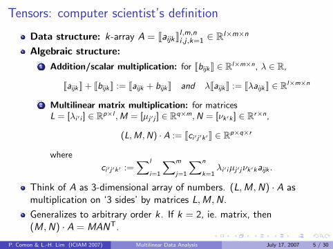
Tensors: computer scientist’s definition

Data structure: k-array A = JaijkKl ,m,ni ,j ,k=1 ∈ Rl×m×n

Algebraic structure:

1 Addition/scalar multiplication: for JbijkK ∈ Rl×m×n, λ ∈ R,

JaijkK + JbijkK := Jaijk + bijkK and λJaijkK := JλaijkK ∈ Rl×m×n

2 Multilinear matrix multiplication: for matricesL = [λi ′i ] ∈ Rp×l ,M = [µj′j ] ∈ Rq×m,N = [νk′k ] ∈ Rr×n,

(L,M,N) · A := Jci ′j′k′K ∈ Rp×q×r

where

ci ′j′k′ :=∑l

i=1

∑m

j=1

∑n

k=1λi ′iµj′jνk′kaijk .

Think of A as 3-dimensional array of numbers. (L,M,N) · A asmultiplication on ‘3 sides’ by matrices L,M,N.

Generalizes to arbitrary order k. If k = 2, ie. matrix, then(M,N) · A = MANT.


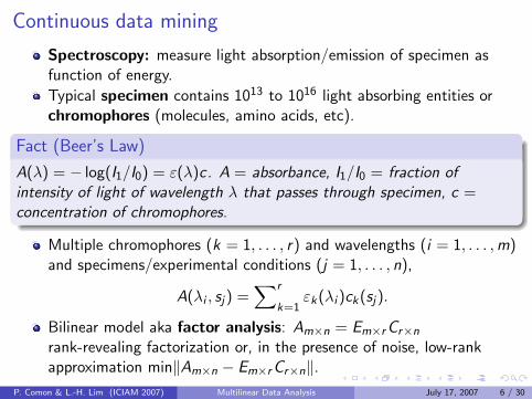
Continuous data mining

Spectroscopy: measure light absorption/emission of specimen asfunction of energy.

Typical specimen contains 1013 to 1016 light absorbing entities orchromophores (molecules, amino acids, etc).

Fact (Beer’s Law)

A(λ) = − log(I1/I0) = ε(λ)c. A = absorbance, I1/I0 = fraction ofintensity of light of wavelength λ that passes through specimen, c =concentration of chromophores.

Multiple chromophores (k = 1, . . . , r) and wavelengths (i = 1, . . . ,m)and specimens/experimental conditions (j = 1, . . . , n),

A(λi , sj) =∑r

k=1εk(λi )ck(sj).

Bilinear model aka factor analysis: Am×n = Em×rCr×n

rank-revealing factorization or, in the presence of noise, low-rankapproximation min‖Am×n − Em×rCr×n‖.


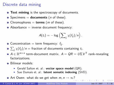
Discrete data mining

Text mining is the spectroscopy of documents.

Specimens = documents (n of these).

Chromophores = terms (m of these).

Absorbance = inverse document frequency:

A(ti ) = − log(∑

jχ(fij)/n

).

Concentration = term frequency: fij .∑j χ(fij)/n = fraction of documents containing ti .

A ∈ Rm×n term-document matrix. A = QR = UΣV T rank-revealingfactorizations.

Bilinear models:

I Gerald Salton et. al.: vector space model (QR);I Sue Dumais et. al.: latent sematic indexing (SVD).

Art Owen: what do we get when m, n →∞?


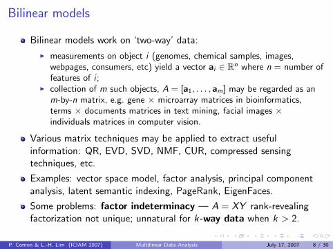
Bilinear models

Bilinear models work on ‘two-way’ data:

I measurements on object i (genomes, chemical samples, images,webpages, consumers, etc) yield a vector ai ∈ Rn where n = number offeatures of i ;

I collection of m such objects, A = [a1, . . . , am] may be regarded as anm-by-n matrix, e.g. gene × microarray matrices in bioinformatics,terms × documents matrices in text mining, facial images ×individuals matrices in computer vision.

Various matrix techniques may be applied to extract usefulinformation: QR, EVD, SVD, NMF, CUR, compressed sensingtechniques, etc.

Examples: vector space model, factor analysis, principal componentanalysis, latent semantic indexing, PageRank, EigenFaces.

Some problems: factor indeterminacy — A = XY rank-revealingfactorization not unique; unnatural for k-way data when k > 2.


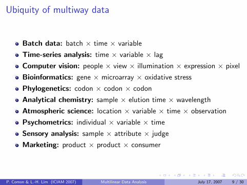
Ubiquity of multiway data

Batch data: batch × time × variable

Time-series analysis: time × variable × lag

Computer vision: people × view × illumination × expression × pixel

Bioinformatics: gene × microarray × oxidative stress

Phylogenetics: codon × codon × codon

Analytical chemistry: sample × elution time × wavelength

Atmospheric science: location × variable × time × observation

Psychometrics: individual × variable × time

Sensory analysis: sample × attribute × judge

Marketing: product × product × consumer


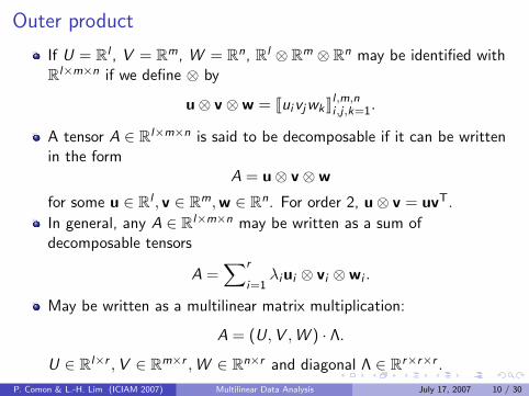
Outer product

If U = Rl , V = Rm, W = Rn, Rl ⊗ Rm ⊗ Rn may be identified withRl×m×n if we define ⊗ by

u⊗ v ⊗w = JuivjwkKl ,m,ni ,j ,k=1.

A tensor A ∈ Rl×m×n is said to be decomposable if it can be writtenin the form

A = u⊗ v ⊗w

for some u ∈ Rl , v ∈ Rm,w ∈ Rn. For order 2, u⊗ v = uvT.

In general, any A ∈ Rl×m×n may be written as a sum ofdecomposable tensors

A =∑r

i=1λiui ⊗ vi ⊗wi .

May be written as a multilinear matrix multiplication:

A = (U,V ,W ) · Λ.

U ∈ Rl×r ,V ∈ Rm×r ,W ∈ Rn×r and diagonal Λ ∈ Rr×r×r .


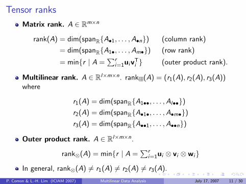
Tensor ranks

Matrix rank. A ∈ Rm×n

rank(A) = dim(spanR{A•1, . . . ,A•n}) (column rank)

= dim(spanR{A1•, . . . ,Am•}) (row rank)

= min{r | A =∑r

i=1uivTi } (outer product rank).

Multilinear rank. A ∈ Rl×m×n. rank�(A) = (r1(A), r2(A), r3(A))where

r1(A) = dim(spanR{A1••, . . . ,Al••})r2(A) = dim(spanR{A•1•, . . . ,A•m•})r3(A) = dim(spanR{A••1, . . . ,A••n})

Outer product rank. A ∈ Rl×m×n.

rank⊗(A) = min{r | A =∑r

i=1ui ⊗ vi ⊗wi}

In general, rank⊗(A) 6= r1(A) 6= r2(A) 6= r3(A).


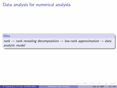
Data analysis for numerical analysts

Idea

rank → rank revealing decomposition → low-rank approximation → dataanalytic model


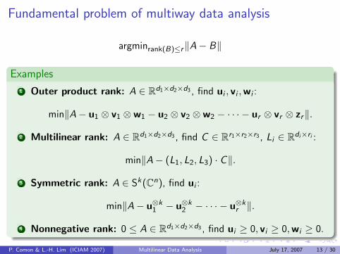
Fundamental problem of multiway data analysis

argminrank(B)≤r‖A− B‖

Examples

1 Outer product rank: A ∈ Rd1×d2×d3 , find ui , vi ,wi :

min‖A− u1 ⊗ v1 ⊗w1 − u2 ⊗ v2 ⊗w2 − · · · − ur ⊗ vr ⊗ zr‖.

2 Multilinear rank: A ∈ Rd1×d2×d3 , find C ∈ Rr1×r2×r3 , Li ∈ Rdi×ri :

min‖A− (L1, L2, L3) · C‖.

3 Symmetric rank: A ∈ Sk(Cn), find ui :

min‖A− u⊗k1 − u⊗k

2 − · · · − u⊗kr ‖.

4 Nonnegative rank: 0 ≤ A ∈ Rd1×d2×d3 , find ui ≥ 0, vi ≥ 0,wi ≥ 0.


Feature revelation

More generally, D = dictionary. Minimal r with

A ≈ α1B1 + · · ·+ αrBr ∈ Dr .

Bi ∈ D often reveal features of the dataset A.

Examples

1 parafac: D = {A ∈ Rd1×d2×d3 | rank⊗(A) ≤ 1}.2 Tucker: D = {A ∈ Rd1×d2×d3 | rank�(A) ≤ (1, 1, 1)}.3 De Lathauwer: D = {A ∈ Rd1×d2×d3 | rank�(A) ≤ (r1, r2, r3)}.4 ICA: D = {A ∈ Sk(Cn) | rankS(A) ≤ 1}.5 NTF: D = {A ∈ Rd1×d2×d3

+ | rank+(A) ≤ 1}.


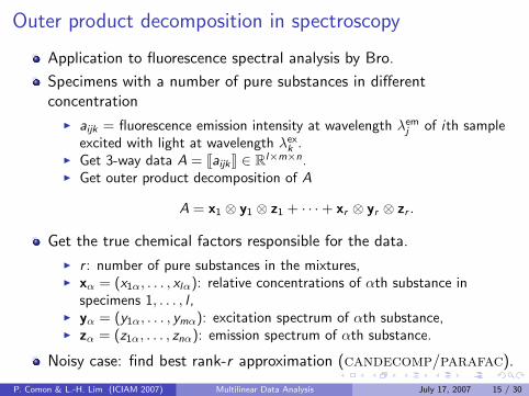
Outer product decomposition in spectroscopy

Application to fluorescence spectral analysis by Bro.

Specimens with a number of pure substances in differentconcentration

I aijk = fluorescence emission intensity at wavelength λemj of ith sample

excited with light at wavelength λexk .

I Get 3-way data A = JaijkK ∈ Rl×m×n.I Get outer product decomposition of A

A = x1 ⊗ y1 ⊗ z1 + · · ·+ xr ⊗ yr ⊗ zr .

Get the true chemical factors responsible for the data.

I r : number of pure substances in the mixtures,I xα = (x1α, . . . , xlα): relative concentrations of αth substance in

specimens 1, . . . , l ,I yα = (y1α, . . . , ymα): excitation spectrum of αth substance,I zα = (z1α, . . . , znα): emission spectrum of αth substance.

Noisy case: find best rank-r approximation (candecomp/parafac).


Multilinear decomposition in bioinformatics

Application to cell cycle studies by Alter and Omberg.

Collection of gene-by-microarray matrices A1, . . . ,Al ∈ Rm×n

obtained under varying oxidative stress.

I aijk = expression level of jth gene in kth microarray under ith stress.I Get 3-way data array A = JaijkK ∈ Rl×m×n.I Get multilinear decomposition of A

A = (X ,Y ,Z ) · C ,

to get orthogonal matrices X ,Y ,Z and core tensor C by applying SVDto various ’flattenings’ of A.

Column vectors of X ,Y ,Z are ‘principal components’ or‘parameterizing factors’ of the spaces of stress, genes, andmicroarrays; C governs interactions between these factors.

Noisy case: approximate by discarding small cijk (Tucker Model).


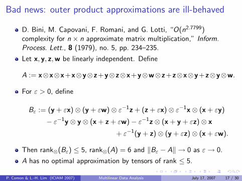
Bad news: outer product approximations are ill-behaved

D. Bini, M. Capovani, F. Romani, and G. Lotti, “O(n2.7799)complexity for n × n approximate matrix multiplication,” Inform.Process. Lett., 8 (1979), no. 5, pp. 234–235.

Let x, y, z,w be linearly independent. Define

A := x⊗x⊗x+x⊗y⊗z+y⊗z⊗x+y⊗w⊗z+z⊗x⊗y+z⊗y⊗w.

For ε > 0, define

Bε := (y + εx)⊗ (y + εw)⊗ ε−1z + (z + εx)⊗ ε−1x⊗ (x + εy)

− ε−1y ⊗ y ⊗ (x + z + εw)− ε−1z⊗ (x + y + εz)⊗ x

+ ε−1(y + z)⊗ (y + εz)⊗ (x + εw).

Then rank⊗(Bε) ≤ 5, rank⊗(A) = 6 and ‖Bε − A‖ → 0 as ε→ 0.

A has no optimal approximation by tensors of rank ≤ 5.


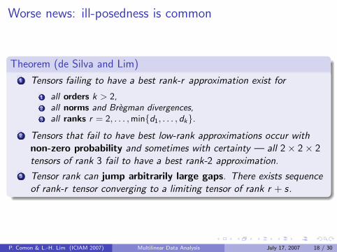
Worse news: ill-posedness is common

Theorem (de Silva and Lim)

1 Tensors failing to have a best rank-r approximation exist for

1 all orders k > 2,2 all norms and Bregman divergences,3 all ranks r = 2, . . . ,min{d1, . . . , dk}.

2 Tensors that fail to have best low-rank approximations occur withnon-zero probability and sometimes with certainty — all 2× 2× 2tensors of rank 3 fail to have a best rank-2 approximation.

3 Tensor rank can jump arbitrarily large gaps. There exists sequenceof rank-r tensor converging to a limiting tensor of rank r + s.


Message

That the best rank-r approximation problem for tensors has nosolution poses serious difficulties.

Incorrect to think that if we just want an ‘approximate solution’, thenthis doesn’t matter.

If there is no solution in the first place, then what is it that are wetrying to approximate? ie. what is the ‘approximate solution’ anapproximate of?

Problems near an ill-posed problem are generally ill-conditioned.


CP degeneracy

CP degeneracy: the phenomenon that individual rank-1 terms inparafac solutions sometime diverges to infinity but in a way thatthe sum remains finite.

Example: minimize ‖A− u⊗ v⊗w− x⊗ y⊗ z‖ via, say, alternatingleast squares,

‖uk ⊗ vk ⊗wk‖ and ‖xk ⊗ yk ⊗ zk‖ → ∞

but not‖uk ⊗ vk ⊗wk + xk ⊗ yk ⊗ zk‖.

If a sequence of rank-r tensors converges to a limiting tensor of rank> r , then all rank-1 terms must become unbounded [de Silva and L].

In other words, rank jumping always imply CP degeneracy.


Some good news: separation rank avoids this problem

G. Beylkin and M.J. Mohlenkamp, “Numerical operator calculus inhigher dimensions,” Proc. Natl. Acad. Sci., 99 (2002), no. 16, pp.10246–10251.

Given ε, find small r(ε) ∈ N so that

‖A− u1 ⊗ v1 ⊗w1 − u2 ⊗ v2 ⊗w2 − · · · − ur(ε) ⊗ vr(ε) ⊗ zr(ε)‖ < ε.

Great for compressing A.

However, data analytic models sometime require a fixed,predetermined r .


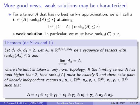
More good news: weak solutions may be characterized

For a tensor A that has no best rank-r approximation, we will call aC ∈ {A | rank⊗(A) ≤ r} attaining

inf{‖C − A‖ | rank⊗(A) ≤ r}a weak solution. In particular, we must have rank⊗(C ) > r .

Theorem (de Silva and L)

Let d1, d2, d3 ≥ 2. Let An ∈ Rd1×d2×d3 be a sequence of tensors withrank⊗(An) ≤ 2 and

limn→∞

An = A,

where the limit is taken in any norm topology. If the limiting tensor A hasrank higher than 2, then rank⊗(A) must be exactly 3 and there exist pairsof linearly independent vectors x1, y1 ∈ Rd1 , x2, y2 ∈ Rd2 , x3, y3 ∈ Rd3

such that

A = x1 ⊗ x2 ⊗ y3 + x1 ⊗ y2 ⊗ x3 + y1 ⊗ x2 ⊗ x3.

Observation 1: a sequence of order-3 rank-2 tensors cannot ‘jumprank’ by more than 1Observation 2: requires exactly six vectors to define, ‘rank-2 like’x1 ⊗ x2 ⊗ x3 + y1 ⊗ y2 ⊗ y3


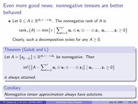
Even more good news: nonnegative tensors are betterbehaved

Let 0 ≤ A ∈ Rd1×···×dk . The nonnegative rank of A is

rank+(A) := min{r

∣∣ ∑r

i=1ui ⊗ vi ⊗ · · · ⊗ zi , ui , . . . , zi ≥ 0

}Clearly, such a decomposition exists for any A ≥ 0.

Theorem (Golub and L)

Let A = Jaj1···jk K ∈ Rd1×···×dk be nonnegative. Then

inf{∥∥A−

∑r

i=1ui ⊗ vi ⊗ · · · ⊗ zi

∥∥ ∣∣ ui , . . . , zi ≥ 0}

is always attained.

Corollary

Nonnegative tensor approximation always have solutions.


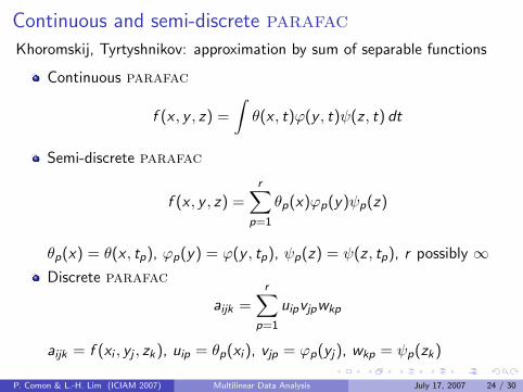
Continuous and semi-discrete parafac

Khoromskij, Tyrtyshnikov: approximation by sum of separable functions

Continuous parafac

f (x , y , z) =

∫θ(x , t)ϕ(y , t)ψ(z , t) dt

Semi-discrete parafac

f (x , y , z) =r∑

p=1

θp(x)ϕp(y)ψp(z)

θp(x) = θ(x , tp), ϕp(y) = ϕ(y , tp), ψp(z) = ψ(z , tp), r possibly ∞Discrete parafac

aijk =r∑

p=1

uipvjpwkp

aijk = f (xi , yj , zk), uip = θp(xi ), vjp = ϕp(yj), wkp = ψp(zk)


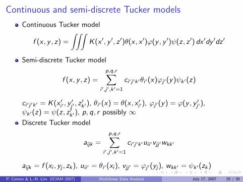
Continuous and semi-discrete Tucker models

Continuous Tucker model

f (x , y , z) =

∫∫∫K (x ′, y ′, z ′)θ(x , x ′)ϕ(y , y ′)ψ(z , z ′) dx ′dy ′dz ′

Semi-discrete Tucker model

f (x , y , z) =

p,q,r∑i ′,j ′,k ′=1

ci ′j ′k ′θi ′(x)ϕj ′(y)ψk ′(z)

ci ′j ′k ′ = K (x ′i ′ , y′j ′ , z

′k ′), θi ′(x) = θ(x , x ′i ′), ϕj ′(y) = ϕ(y , y ′j ′),

ψk ′(z) = ψ(z , z ′k ′), p, q, r possibly ∞Discrete Tucker model

aijk =

p,q,r∑i ′,j ′,k ′=1

ci ′j ′k ′uii ′vjj ′wkk ′

aijk = f (xi , yj , zk), uii ′ = θi ′(xi ), vjj ′ = ϕj ′(yj), wkk ′ = ψk ′(zk)


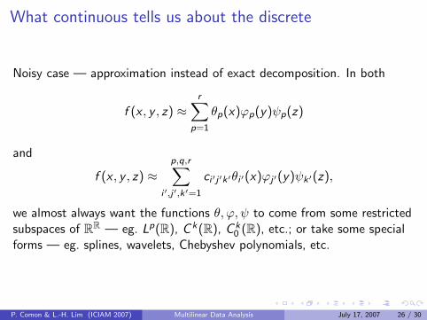
What continuous tells us about the discrete

Noisy case — approximation instead of exact decomposition. In both

f (x , y , z) ≈r∑

p=1

θp(x)ϕp(y)ψp(z)

and

f (x , y , z) ≈p,q,r∑

i ′,j ′,k ′=1

ci ′j ′k ′θi ′(x)ϕj ′(y)ψk ′(z),

we almost always want the functions θ, ϕ, ψ to come from some restrictedsubspaces of RR — eg. Lp(R), C k(R), C k

0 (R), etc.; or take some specialforms — eg. splines, wavelets, Chebyshev polynomials, etc.


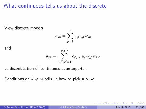
What continuous tells us about the discrete

View discrete models

aijk =r∑

p=1

uipvjpwkp

and

aijk =

p,q,r∑i ′,j ′,k ′=1

ci ′j ′k ′uii ′vjj ′wkk ′

as discretization of continuous counterparts.

Conditions on θ, ϕ, ψ tells us how to pick u, v,w.


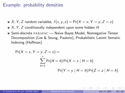
Example: probability densities

X ,Y ,Z random variables, f (x , y , z) = Pr(X = x ,Y = y ,Z = z)

X ,Y ,Z conditionally independent upon some hidden H

Semi-discrete parafac — Naıve Bayes Model, Nonnegative TensorDecomposition (Lee & Seung, Paatero), Probabilistic Latent SematicIndexing (Hoffman)

Pr(X = x ,Y = y ,Z = z) =r∑

h=1

Pr(H = h) Pr(X = x | H = h)

Pr(Y = y | H = h) Pr(Z = z | H = h)


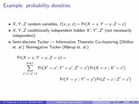
Example: probability densities

X ,Y ,Z random variables, f (x , y , z) = Pr(X = x ,Y = y ,Z = z)

X ,Y ,Z conditionally independent hidden X ′,Y ′,Z ′ (not necessarilyindependent)

Semi-discrete Tucker — Information Theoretic Co-clustering (Dhillonet. al.) Nonnegative Tucker (Mørup et. al.)

Pr(X = x ,Y = y ,Z = z) =p,q,r∑

x ′,y ′,z ′=1

Pr(X ′ = x ′,Y ′ = y ′,Z ′ = z ′) Pr(X = x | X ′ = x ′)

Pr(Y = y | Y ′ = y ′) Pr(Z = z | Z ′ = z ′)


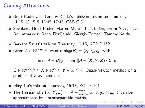
Coming Attractions

Brett Bader and Tammy Kolda’s minisympoisum on Thursday,11:15–13:15 & 15:45–17:45, CAB G 51

Speakers: Brett Bader, Morten Mørup, Lars Elden, Evrim Acar, LievenDe Lathauwer, Derry FitzGerald, Giorgio Tomasi, Tammy Kolda

Berkant Savas’s talk on Thursday, 11:15, KO2 F 172

Given A ∈ Rl×m×n, want rank�(B) = (r1, r2, r3) with

min ‖A− B‖F = min ‖A− (X ,Y ,Z ) · C‖F

C ∈ Rr1×r2×r3 , X ∈ Rl×r1 , Y ∈ Rm×r2 . Quasi-Newton method on aproduct of Grassmannians.

Ming Gu’s talk on Thursday, 16:15, KOL F 101

The Hessian of F (X ,Y ,Z ) = ‖A−∑r

α=1xα ⊗ yα ⊗ zα‖2F can be

approximated by a semiseparable matrix.


multilinear algebra in machine learning and signal processing

Documents