multilevel regression models for mean and (co)variance · 2016-03-10 · multilevel regression...
TRANSCRIPT

Multilevel Regression Modelsfor Mean and (Co)variance
with Applications in Nursing Research
Baoyue Li

Multilevel Regression Models for Mean and (Co)variancewith applications in nursing research
Multilevel regressie modellen voor mean en (co)variantiemet toepassingen in verplegingswetenschap
Proefschrift
ter verkrijging van de graad van doctor aan deErasmus Universiteit Rotterdamop gezag van de rector magnificus
Prof.dr. H.A.P. Pols
en volgens besluit van het College voor Promoties
De openbare verdediging zal plaatsvinden opdinsdag 17 juni 2014 om 13:30 uur
door
Baoyue Li
geboren te LiaoNing, China

Promotiecommissie
Promotor
Prof.dr. E.M.E.H. Lesaffre
Overige leden
Prof.dr. E.W. SteyerbergProf.dr. L.R. ArendsProf.dr. W. Sermeus

To my wife, my parents and my sisters

CONTENTS
Chapter 1 General introduction 1
1.1 Introduction . . . . . . . . . . . . . . . . . . . . . . . . . . . . . . . . . 31.2 Hierarchical data . . . . . . . . . . . . . . . . . . . . . . . . . . . . . . . 31.3 Mixed effects models . . . . . . . . . . . . . . . . . . . . . . . . . . . . 31.4 Estimation methods . . . . . . . . . . . . . . . . . . . . . . . . . . . . . 61.5 Factor analytic models . . . . . . . . . . . . . . . . . . . . . . . . . . . 101.6 Structural equation modeling . . . . . . . . . . . . . . . . . . . . . . . 13
Chapter 2 Aims and outline of the thesis 15
2.1 Introduction . . . . . . . . . . . . . . . . . . . . . . . . . . . . . . . . . 172.2 Motivating data set . . . . . . . . . . . . . . . . . . . . . . . . . . . . . 172.3 Clinical aims . . . . . . . . . . . . . . . . . . . . . . . . . . . . . . . . . 172.4 Statistical aims . . . . . . . . . . . . . . . . . . . . . . . . . . . . . . . . 172.5 Outline of the thesis . . . . . . . . . . . . . . . . . . . . . . . . . . . . . 18
Chapter 3 Logistic random effects regression models: A comparison of statistical
packages for binary and ordinal outcomes 21
3.1 Background . . . . . . . . . . . . . . . . . . . . . . . . . . . . . . . . . 233.2 Methods . . . . . . . . . . . . . . . . . . . . . . . . . . . . . . . . . . . 243.3 Results . . . . . . . . . . . . . . . . . . . . . . . . . . . . . . . . . . . . 293.4 Discussion . . . . . . . . . . . . . . . . . . . . . . . . . . . . . . . . . . 443.5 Conclusions . . . . . . . . . . . . . . . . . . . . . . . . . . . . . . . . . 48
Chapter 4 A multi-country perspective on nurses tasks below their skill level: Re-
ports from domestically trained nurses and foreign trained nurses from
developing countries 51
4.1 Background . . . . . . . . . . . . . . . . . . . . . . . . . . . . . . . . . 534.2 Methods . . . . . . . . . . . . . . . . . . . . . . . . . . . . . . . . . . . 544.3 Findings . . . . . . . . . . . . . . . . . . . . . . . . . . . . . . . . . . . 564.4 Discussion . . . . . . . . . . . . . . . . . . . . . . . . . . . . . . . . . . 604.5 Conclusion . . . . . . . . . . . . . . . . . . . . . . . . . . . . . . . . . . 63
Contents
Chapter 5 Nursing unit managers and staff nurses opinions of the nursing work
environment: A Bayesian multilevel MIMIC model for cross-group com-
parisons 65
5.1 Introduction . . . . . . . . . . . . . . . . . . . . . . . . . . . . . . . . . 67
5.2 Method . . . . . . . . . . . . . . . . . . . . . . . . . . . . . . . . . . . . 68
5.3 Results . . . . . . . . . . . . . . . . . . . . . . . . . . . . . . . . . . . . 72
5.4 Discussion . . . . . . . . . . . . . . . . . . . . . . . . . . . . . . . . . . 75
5.5 Conclusion . . . . . . . . . . . . . . . . . . . . . . . . . . . . . . . . . . 78
Chapter 6 Group-level impact of work environment dimensions on burnout experi-
ences among nurses: A multivariate multilevel probit model 83
6.1 Background . . . . . . . . . . . . . . . . . . . . . . . . . . . . . . . . . 85
6.2 Methods . . . . . . . . . . . . . . . . . . . . . . . . . . . . . . . . . . . 86
6.3 Results . . . . . . . . . . . . . . . . . . . . . . . . . . . . . . . . . . . . 91
6.4 Discussion . . . . . . . . . . . . . . . . . . . . . . . . . . . . . . . . . . 96
6.5 Conclusions . . . . . . . . . . . . . . . . . . . . . . . . . . . . . . . . . 100
Appendix . . . . . . . . . . . . . . . . . . . . . . . . . . . . . . . . . . . . . 103
Chapter 7 A multivariate multilevel Gaussian model with a mixed effects structure
in the mean and covariance part 105
7.1 Introduction . . . . . . . . . . . . . . . . . . . . . . . . . . . . . . . . . 107
7.2 Motivating data set: the RN4CAST project . . . . . . . . . . . . . . . . 109
7.3 A single factor Model . . . . . . . . . . . . . . . . . . . . . . . . . . . . 113
7.4 Multiple factors model . . . . . . . . . . . . . . . . . . . . . . . . . . . 120
7.5 Computational procedure . . . . . . . . . . . . . . . . . . . . . . . . . . 121
7.6 Missing data . . . . . . . . . . . . . . . . . . . . . . . . . . . . . . . . . 121
7.7 Analysis of the RN4CAST burnout data . . . . . . . . . . . . . . . . . . 123
7.8 Simulation study . . . . . . . . . . . . . . . . . . . . . . . . . . . . . . . 130
7.9 Discussion . . . . . . . . . . . . . . . . . . . . . . . . . . . . . . . . . . 131
Appendix . . . . . . . . . . . . . . . . . . . . . . . . . . . . . . . . . . . . . 136
Chapter 8 Multilevel Higher Order Factor Model: Joint modeling of a multilevel
factor analytic model and a multilevel covariance regression model 141
8.1 Introduction . . . . . . . . . . . . . . . . . . . . . . . . . . . . . . . . . 143
8.2 Motivating Data set . . . . . . . . . . . . . . . . . . . . . . . . . . . . . 144
8.3 Proposed model . . . . . . . . . . . . . . . . . . . . . . . . . . . . . . . 149
8.4 Computational procedure . . . . . . . . . . . . . . . . . . . . . . . . . . 154
8.5 Comparison of the two-stage approach and the MHOF model: a lim-ited simulation study . . . . . . . . . . . . . . . . . . . . . . . . . . . . 155
8.6 Application to the RN4CAST data set . . . . . . . . . . . . . . . . . . . 155
8.7 Conclusions . . . . . . . . . . . . . . . . . . . . . . . . . . . . . . . . . 163

Contents
Chapter 9 Conclusions 167
9.1 General conclusions . . . . . . . . . . . . . . . . . . . . . . . . . . . . . 1699.2 Future research . . . . . . . . . . . . . . . . . . . . . . . . . . . . . . . . 170


1GENERAL INTRODUCTION
1


1.1 Introduction
1.1 Introduction
In this chapter, a concise overview is provided for the statistical techniques that are appliedin this thesis. This includes two classes of statistical modeling approaches which have beencommonly applied in plenty of research areas for many decades. Namely, we will describethe fundamental ideas about mixed effects models and factor analytic (FA) models. To bespecific, this chapter covers several types of these two classes of modeling approaches. Forthe mixed effects models, we briefly describe the linear, generalized and multivariate mixedeffects models, while for the FA models, exploratory FA (EFA), confirmatory FA (CFA) mod-els and multilevel FA (MFA) models are covered. As an extension of FA models, structuralequation modeling (SEM) and multilevel SEM are also briefly described. we also discussthe two classical estimating methods, i.e. the frequentist and the Bayesian approach, withthe latter chosen as the analytic algorithm for our proposed models.
1.2 Hierarchical data
Hierarchical (also called multilevel or clustered) data are abundantly present in empiricalresearch. For example, a quality of life survey collects information of residents from eachhousehold; a clinical trial recruits patients from multiple medical centers; an evaluation ofthe teaching quality samples students from different schools; a rehabilitation test recordsdaily patients’ performance for a certain period; etc. An important feature of all these kindsof multilevel structured data is ”non-independence”, e.g. residents from the same house-hold tend to act more similar than those from different households as they share the samehousehold environment and are genetically related. The data set used in most chapters ofthis thesis is taken from a multi-country European nurse survey, the RN4CAST (registerednurse forecasting) project. This project involved a large number of nurses within nursingunits within hospitals across countries, implying a four-level hierarchical structure. Feelingsof work-related burnout, measured with the multidimensional 22-item Maslach BurnoutInventory (MBI, (Maslach and Jackson, 1981)), are examined in this thesis with relation towork environment variables and personal characteristics. Three dimensions were extractedby Maslach and Jackson (1981) using a factor analytic model.
1.3 Mixed effects models
1.3.1 Linear mixed effects models
Linear mixed effects models (LMM) are linear models with both fixed and random effects.A specific case of a LMM is a longitudinal growth study, where the baseline responses forthe individuals differ but their linear growth is the same. This yields the random interceptsmodel, given by:
yij = βTxij + uj + εij , i = 1, 2, ..., nj ; j = 1, 2, ..., k,
uj ∼ N(0, σ2u), εij ∼ N(0, σ2
ε), uj ⊥ εij ,(1.1)
3
Chapter 1 General introduction
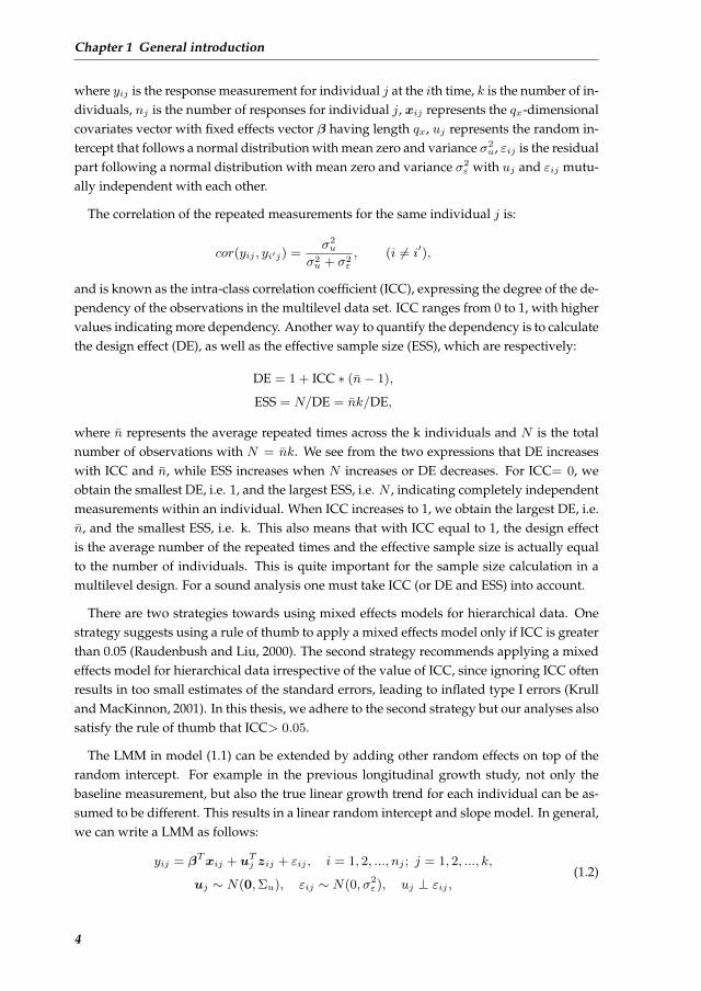
where yij is the response measurement for individual j at the ith time, k is the number of in-dividuals, nj is the number of responses for individual j, xij represents the qx-dimensionalcovariates vector with fixed effects vector β having length qx, uj represents the random in-tercept that follows a normal distribution with mean zero and variance σ2
u, εij is the residualpart following a normal distribution with mean zero and variance σ2
ε with uj and εij mutu-ally independent with each other.
The correlation of the repeated measurements for the same individual j is:
cor(yij , yi′j) =σ2u
σ2u + σ2
ε
, (i 6= i′),
and is known as the intra-class correlation coefficient (ICC), expressing the degree of the de-pendency of the observations in the multilevel data set. ICC ranges from 0 to 1, with highervalues indicating more dependency. Another way to quantify the dependency is to calculatethe design effect (DE), as well as the effective sample size (ESS), which are respectively:
DE = 1 + ICC ∗ (n− 1),
ESS = N/DE = nk/DE,
where n represents the average repeated times across the k individuals and N is the totalnumber of observations with N = nk. We see from the two expressions that DE increaseswith ICC and n, while ESS increases when N increases or DE decreases. For ICC= 0, weobtain the smallest DE, i.e. 1, and the largest ESS, i.e. N , indicating completely independentmeasurements within an individual. When ICC increases to 1, we obtain the largest DE, i.e.n, and the smallest ESS, i.e. k. This also means that with ICC equal to 1, the design effectis the average number of the repeated times and the effective sample size is actually equalto the number of individuals. This is quite important for the sample size calculation in amultilevel design. For a sound analysis one must take ICC (or DE and ESS) into account.
There are two strategies towards using mixed effects models for hierarchical data. Onestrategy suggests using a rule of thumb to apply a mixed effects model only if ICC is greaterthan 0.05 (Raudenbush and Liu, 2000). The second strategy recommends applying a mixedeffects model for hierarchical data irrespective of the value of ICC, since ignoring ICC oftenresults in too small estimates of the standard errors, leading to inflated type I errors (Krulland MacKinnon, 2001). In this thesis, we adhere to the second strategy but our analyses alsosatisfy the rule of thumb that ICC> 0.05.
The LMM in model (1.1) can be extended by adding other random effects on top of therandom intercept. For example in the previous longitudinal growth study, not only thebaseline measurement, but also the true linear growth trend for each individual can be as-sumed to be different. This results in a linear random intercept and slope model. In general,we can write a LMM as follows:
yij = βTxij + uTj zij + εij , i = 1, 2, ..., nj ; j = 1, 2, ..., k,
uj ∼ N(0,Σu), εij ∼ N(0, σ2ε), uj ⊥ εij ,
(1.2)
4
1.3 Mixed effects models
where uj represents the qz-dimensional random effect with a multivariate normal distri-bution having mean zero and covariance matrix Σu, zij is the corresponding qz covariatesvector. The other terms are the same as in model (1.1). Note that zij may be different fromxij . Model (1.1) is obtained when zij has a single value 1. A specific case of model (1.2) isthe cross-classified mixed effects model. This model arises when there exist more than onehierarchical structure for the data, e.g. students come from different schools and differentdistricts where both school and district are clusters but are not nested within each other.
1.3.2 Generalized linear mixed models
The LMM is a special case of a generalized LMM (GLMM) whereby the response has anormal distribution with an identity link function. In general, the GLMM can handle alarge amount of probability distributions coming from the exponential family such as thenormal, binomial, Poisson and gamma distributions up to random effects. For a GLMM, itis assumed that the expected value of the response yij can be modeled as a linear functionof fixed and random effects up to a link function g(), i.e.:
g(E(yij |uj)) = βTxij + uTj zij , i = 1, 2, ..., nj ; j = 1, 2, ..., k,
uj ∼ N(0,Σu),(1.3)
whereby uj is usually assigned a multivariate normal distribution, but other distributionssuch as a multivariate t distribution are possible. GLMMs have been suggested to addressthe overdispersion of e.g. count responses (Breslow, 1984).
When the response has a binomial distribution with a logit link function, we obtain alogistic mixed effects model, where:
E(yij |uj) = pij =eβ
T xij+uTj zij
1 + eβT xij+uT
j zij, (1.4)
where pij represents the conditional expected probability for the observed binomial data.The right-hand side part of model (1.4) is actually known as the logistic function of βTxij +
uTj zij . An alternative to the logistic model for the binomial data is the probit model, withthe probit link function having the form:
pij = Φ(βTxij + uTj zij), (1.5)
where Φ is the cumulative distribution function (CDF) of a standard normal distribution.It has been shown that the parameter estimates from the logistic and probit models aresimilar up to a constant value, i.e. the coefficients from a logistic model are 1.6 times of thecorresponding ones under a probit link model (Gelman and Hill, 2006).
5
Chapter 1 General introduction
1.3.3 Multivariate mixed effects models
The multivariate mixed effects model is the generalization of the mixed effects model tomultiple responses at the same time. The multivariate LMM has the following form:
yij = Bxij +U jzij + εij , i = 1, 2, ..., nj ; j = 1, 2, ..., k,
U j ∼ N(0,Σu), εij ∼ N(0,Σε), U j ⊥ εij ,(1.6)
where yij represents the p-dimensional response vector for individual i from group j. Thecovariates xij and zij have the same meaning as in model (1.2), and now with the fixedand random effects being a p × qx matrix B and a p × qz matrix U j , respectively. Thep-dimensional residual vector εij is usually assumed to have a multivariate normal distri-bution with mean zero and the covariance matrix Σε.
We see from model (1.6) that the correlated nature of the responses is reflected by corre-lated residuals and correlated random effects. The latter means that not only the randomeffects within each response are correlated, but also the random effects across the responsesare correlated. This may increase the power for estimation because the parameter estimatesfor each of the p responses can borrow information from each other through the correlations.In addition, tests for the equality of the parameter estimates across multiple responses andglobal tests based on all responses can be constructed. Take the three-dimensional burnoutmeasurements as an example. Through a multivariate linear random effects model withthe covariate work environment, we can test whether the effects of work environment are thesame for all the three burnout dimensions taking into account the multilevel structure. Wecan also check whether the work environment variable has a significant effect on all of thethree burnout dimensions simultaneously, thereby dealing with the multiple testing prob-lem.
1.4 Estimation methods
Generally speaking, there are two main classes of estimating methods: the frequentist ap-proach and the Bayesian approach. In this section, we describe some basic features of eachapproach and the performance of these two approaches for handling some of the modelsmentioned earlier.
1.4.1 Frequentist approach
In the frequentist approach, probability is defined as a limiting relative frequency. Thatis, the probability of an event is the limit of the relative frequency of that event in a largenumber of studies. Further, in frequentist statistics one estimates the unknown but fixedmodel parameter θ. Prediction is done given the estimated θ and the uncertainty of theprediction is based on the sampling property of the estimated value of θ (Feller, 1968).
Maximum likelihood (ML) is a popular way of estimating the model parameters. It findsthe parameter estimates that maximize the likelihood function, L(θ|y) = p(y|θ), thereforeare called the maximum likelihood estimates (MLEs). For many models without random
6
1.4 Estimation methods
effects, the likelihood function is relatively simple and can be written analytically (witha closed form). When the model contains random effects, the marginal likelihood is calcu-lated by integrating over the random effects to obtain the MLEs. For example for a LMM ex-pressed in model (1.2), let θ denote all parameters except the random effects, i.e. (β,Σu, σ
2ε),
the marginal likelihood is:
Lm(θ,y) = p(y|β,Σu, σ2ε)
=
k∏j=1
∫ nj∏i=1
p(yij |β, σ2ε ,uj)p(uj |Σu)duj . (1.7)
The integral in this expression can be solved analytically, and the likelihood function iswritten as:
Lm(θ,y) =
k∏j=1
{(2π)−nj/2|Vj |−1/2 × exp(−1
2(yj −Xjβ)TV −1
j (yj −Xjβ))}, (1.8)
where yj represents the response vector for group j with length nj , N is the total number
of individuals (N =k∑j=1
nj), β is the qx-dimensional fixed effects vector with Xj its cor-
responding covariate matrix of dimension nj × qx, Vj is the nj × nj marginal covariancematrix of yj , which has the form:
Vj = ZjΣuZTj + σ2
εI.
In this form Zj is the corresponding nj × qz covariate matrix for the random effects havinga qz × qz covariance matrix Σu, and I is the identity matrix of size nj .
Unfortunately, for most of the GLMMs such as the logistic random effects models, thereexists no closed form for the likelihood function (1.7). To solve this, numerical approxima-tions have been developed, e.g. the non-adaptive Gaussian quadrature method, the adap-tive Gaussian quadrature method with the Laplacian approximation as the simplest case,etc. Further, based on the approximated marginal likelihood function, the maximizationalgorithms such as the Newton-Raphson and the iterative generalized least square (IGLS)algorithms, are required to find the MLEs.
1.4.2 Bayesian approach
In the Bayesian approach the parameter θ is given a probability distribution which ex-presses our prior knowledge about that parameter. There is still a true value for the pa-rameter (Lesaffre and Lawson, 2012), but the parameter becomes stochastic because of ouruncertainty of its value. We denote p(θ) as the prior distribution of θ obtained from expertknowledge, historical information, etc., but without observing the current data y. L(θ|y) isthe likelihood defined by the model specification. The probability distribution of θ obtainedfrom combining the information from the prior and the data is given by Bayes’ Theorem
7
Chapter 1 General introduction
and is called the posterior distribution given by:
p(θ|y) =L(θ|y)p(θ)
p(y)=
L(θ|y)p(θ)∫L(θ|y)p(θ)dθ
. (1.9)
The denominator p(y) can be written as the integration of the likelihood L(θ|y) over thevariable θ, therefore is called the averaged likelihood. Bayes’ Theorem shows one of theadvantages of the Bayesian approach, namely that it can utilize the informative prior whichmay increase the power for estimation. For example, previous similar studies could be usedto represent our prior belief when analyzing the data from the current study, which mayresult in a more precise conclusion. However informative priors have also caused a lot ofcontroversy between Bayesians and frequentists, since frequentists accused the Bayesianapproach to be subjective. When no prior information is available, a non-informative priorcould be used. Then, the likelihood dominates the prior and information from the posterioris actually equivalent to the information extracted from the likelihood.
Bayesian estimation involves integration as shown in Bayes’ Theorem. The denomina-tor may involve high-dimensional integration for the joint posterior distribution of high-dimensional parameters as the Bayesian method treats all parameters as random variables.This integration becomes even heavier in the presence of random effects or latent variables.For the LMM of model (1.1), the joint posterior distribution of all parameters, including therandom effects u, is then:
p(β,Σu, σ2ε ,u|y) =
L(β,Σu, σ2ε ,u|y)p(u|Σu)p(β)p(Σu)p(σ2
ε)
p(y)
=p(y|β, σ2
ε ,u)p(u|Σu)p(β)p(Σu)p(σ2ε)∫
β
∫Σu
∫σ2ε
∫uL(y|β, σ2
ε ,u)p(u|Σu)p(β)p(Σu)p(σ2ε)dβdΣudσ2
εdu.
Note that in the denominator, each integral may involve multiple integrations dependingon their respective dimensions. Because of the high-dimensional integration, the Bayesianapproach was for about two centuries impossible to use for real-life problems (Lesaffre andLawson, 2012).
1.4.2.1 Bayesian computational techniques
In 1990, a powerful class of numerical procedures, called Markov Chain Monte Carlo (MCMC)techniques (Gelfand and Smith, 1990), was launched which revolutionized the Bayesian ap-proach. The MCMC technique is based on a sampling approach, i.e. the integral is ap-proximated by Monte Carlo sampling (Ripley, 1987). There are two major classes of MCMCtechniques: Gibbs sampling and Metropolis-Hastings (MH) sampling. We describe hereboth methods but focus on Gibbs sampling which is the most popular approach used forthe considered models in this thesis.
Gibbs sampling Gibbs sampling was first introduced by Geman and Geman (1984) andis commonly used nowadays for Bayesian inference. It explores the M -dimensional jointposterior distributions of θ, and therefore of each parameter θm. This is done by sampling
8

1.4 Estimation methods
from the full conditional distributions p(θm|θ(−m),y), where θ(−m) represents all parame-ters except θm (m = 1, 2, ...,M ). To initialize the updating phase of all parameters in Gibbssampling, a set of starting values are first given to each parameter in θ, denoted as θ0. Forthe first iteration, the Gibbs sampling proceeds as follows:
• Sample θ(1)1 from the full conditional distribution p(θ1|θ0
(−1),y)
• Sample θ(1)2 from the full conditional distribution p(θ2|θ(1)
1 , θ03, ..., θ
0M ,y)
• ...
• Sample θ(1)M from the full conditional distribution p(θM |θ(1)
1 , θ(1)2 , ..., θ
(1)M−1,y)
Thus a new set of values θ(1) = (θ(1)1 , θ
(1)2 , ..., θ
(1)M ) is obtained from the starting values θ0
and the observed data y. The second iteration is conducted based on the new set of valuesθ(1) and the data, and so on so forth. In general, the Gibbs sampling for the mth parameterin the lth iteration is conducted from the following full conditional distribution:
θ(l)m ∼ p(θm|θ
(l)1 , ...θ
(l)m−1, θ
(l−1)m+1 , ..., θ
(l−1)M ,y), m = 1, 2, ...,M, l = 1, 2, ..., L
where M is the total number of parameters and L is the total number of iterations. The iter-ation continues till the Markov chain(s) for each parameter have converged. When multiplechains are launched, convergence can be tested using, e.g. the BGR diagnostic (Brooks andGelman, 1998) which compares the between- and within-chain variability. At the end, weobtain for each parameter L samples. After removing the non-converged part of the chain,called the ”burn-in” part, the remaining samples represent well the marginal posterior dis-tribution for each parameter.
We note that the samples obtained using Gibbs sampling are not independent. Each set ofsamples θ(l) depends on the previous samples θ(l−1) but is conditionally independent withall other previous samples given θ(l−1), i.e.,
p(θ(l)|θ(1), ..., θ(l−1),y) = p(θ(l)|θ(l−1),y).
This is known as the Markov property. Gibbs sampling assumes that the full conditionaldistributions p(θm|θ(−m),y) should be relatively easy to sample from. In cases that the fullconditional distribution is hard to obtain or hard to sample from, we may use a differentsampling algorithm, called the Metropolis-Hastings (MH) algorithm which is described be-low.
Metropolis-Hastings sampling Another class of MCMC sampling methods is the Metropolis-Hastings (MH) algorithm. Here the parameters θ are first sampled from a proposal distri-bution q and in a second step part of the sampled values are accepted to yield a sample fromthe posterior distribution p(θ|y). This involves the following two steps:
1. For iteration l, a candidate sample θ is sampled from q(θ|θ(l)).
9
Chapter 1 General introduction
2. Calculate the acceptance ratio α = p(θ|y)q(θ(l)|θ)
p(θ(l)|y)q(θ|θ(l)) and choose the next sample on:
θ(l+1) =
{θ, with the probability min(1, α);θ(l), otherwise.
Mathematically, Gibbs sampling could be seen as a special type of MH sampling in that theproposal distribution q in Gibbs sampling is the full conditional distribution for each θm
and the acceptance ratio α is always 1.Gibbs sampling, together with many other sampling methods, are nowadays implemented
in many statistical programs and packages, such as WinBUGS (Bayesian inference UsingGibbs Sampling) (Spiegelhalter et al., 2003), JAGS (Just Another Gibbs Sampler) (Plummer,2003), Mplus (Muthen and Muthen, 2010), etc. These programs may differ in the defaultsampling method for a specific type of parameters, thus may behave differently.
1.5 Factor analytic models
A questionnaire is a common research instrument in a survey to collect information aboutsubjects regarding all kinds of behavior, feelings, etc. Take the burnout measurement in theRN4CAST nurse survey as an example. Burnout is a syndrome of emotional exhaustion,depersonalization and reduced personal accomplishment that can occur among individualswho do ”people work” of some kind (Maslach and Jackson, 1986). Burnout is measuredindirectly via a series of questions that reflect all these aspects. In fact, the classic question-naire used for burnout contains the 22-item Maslach Burnout Inventory (MBI, (Maslach andJackson, 1981)) that has proved to measure the above mentioned three dimensions well. Wecall these three dimensions latent constructs, while the 22 items are manifest measures. Therelationship between the latent constructs and the manifest measures is typically studied bya factor analytic (FA) model, which is a special type of a multivariate analysis. FA modelsare classified into two types, i.e. the exploratory FA (EFA) and the confirmatory FA (CFA)model.
EFA and CFA models
The EFA model is usually used to identify a number of latent constructs underlying a rela-tively larger set of observed variables. An EFA model is especially useful when we have noa priori hypothesis on the latent factor structure. Note the difference of an EFA model withprinciple component analysis (PCA) which is an exploratory variable reduction technique.Among other differences, PCA does not assume any particular statistical model for the data,while an EFA model is defined as:
yi = µ+ Lf i + εi, i = 1, 2, ..., N,
f i ∼ N(0,Σf ), εi ∼ N(0,Σε), f i ⊥ εi,(1.10)
where yi represents the p-dimensional response for individual i andµ is the intercept vectorwith the same length p, f i represents the q-dimensional common factors (q < p) following
10
1.5 Factor analytic models
a multivariate normal distribution with covariance matrix Σf and L is the correspondingfactor loading matrix of size p × q, εi is the residual vector for each individual, having amultivariate normal distribution with covariance matrix Σε, it is assumed to be independentwith the common factors and is also called the unique factors in an FA model.
The aim of a CFA model is to test the underlying factor structure that we have a priori inmind. This hypothesis may come from previous studies or is based on theory. A CFA modelcould also represent a further simplification of the factor structure after an EFA model hasbeen fitted. With a reasonable model fit, the CFA model could provide evidence to confirman assumed factor structure. A typical CFA model has the same form as an EFA modelshown in model (1.10). The factor loading matrix L in a CFA model, however, is differentfrom that of an EFA model in that some elements are fixed at constant values. That is, thecross-loadings are fixed to zero since we have in mind a priori a particular factor structureas our testing hypothesis.
For either an EFA or a CFA model, the implied covariance matrix of the observed variabley has the following form:
Σ = LΣfLT + Σε. (1.11)
Note that by implementing a factor model the covariance matrix of the observed responsescould be rebuilt through the factor loadings L, the covariance matrix of factors Σf and thecovariance matrix of residuals Σε.
1.5.1 Identification
The FA model (1.10) resembles a multivariate linear regression model except that f i arenot observed covariates but unknown latent factors. This causes an identification problemmeaning that more than one set of parameter estimates satisfies model (1.10). Further con-straints are required for the common factors f j and/or the loading matrix L, in a CFA andan EFA model.
The identifying constraints for CFA and EFA models are different as they have differentmodel assumptions and are used for different purposes. There are plenty of ways to setthese constraints and here we only display one of them. For a more detailed description ofthe identification issues, we refer to Thompson (2004).
In an EFA model, the following constraints are used in addition for model (1.10):
• Set the covariance matrix for the common factors to be identity: Σf = I .
• Estimate only the diagonal covariance matrix of the unique factors.
This is also called the orthogonal FA model because the common factors are orthogonal witheach other.
For a CFA model, we use the following constraints in model (1.10):
• Fix one loading to 1 for each common factor.
• Estimate only the diagonal covariance matrix for the unique factors.
11

Chapter 1 General introduction
This choice of constraints implies that the general covariance matrix Σf of the commonfactors can be estimated.
Further, we would like to highlight here some of the differences between Bayesian andfrequentist approaches in identifying an FA model. Firstly, for the part Lf in the factormodel, the distribution of the common factors f is usually symmetric with mean zero, e.g.a multivariate normal distribution. This causes a unique identification issue in Bayesianapproach called the ”flipping states” issue (Maydeu-Olivares and McArdle, 2005), wherebyboth L and −L are the solutions for the factor loadings if no further constraints are setfor L. The frequentist approach finds only one of the solutions while the Bayesian ap-proach, which is simulation-based, may move between the two solutions and may neverget converged (Browne, 2012). Further constraints, therefore, are required for Bayesian fac-tor analytic modeling. Secondly, some of the identifying constraints on parameters in thefrequentist approach could be to fix these at a particular value. The same strategy could beapplied in the Bayesian approach, but there is an alternative solution by introducing reason-able informative priors for the parameters needed to constraint (Muthen and Asparouhov,2012). This approach is applied in this thesis.
1.5.2 Multilevel FA model
When the data show a multilevel structure, e.g. nurses within hospitals, the correlated na-ture should also be taken into account in the FA models to obtain valid estimates (Longfordand Muthen, 1992). This gives rise to the multilevel FA (MFA) model. A two-level MFAmodel can be written as:
yij = µ+ LBf j + uj + LWf ij + εij ,
f j ∼ N(0,ΣfB), uj ∼ N(0,Σu),
f ij ∼ N(0,ΣfW ), εij ∼ N(0,Σε),
i = 1, 2, ..., nj ; j = 1, 2, ..., k, f j ⊥ uj ⊥ f ij ⊥ εij ,
(1.12)
where yij represents the p-dimensional response for individual i from group j, f j is the qB-dimensional between-level common factor vector with the factor loading matrix LB havingthe dimension of p× qB , f ij is the qW -dimensional within-level common factor vector withthe factor loading matrixLW having the dimension p×qW ,uj is the p-dimensional between-level unique factor with covariance matrix Σu, εij is the p-dimensional within-level uniquefactor with covariance matrix Σε and all the common and unique factors are assumed mutu-ally independent with each other. The implied covariance matrix for the MFA model (1.12)is then:
Σ = LBΣfBLTB + Σu + LWΣfWL
TW + Σε. (1.13)
12
1.6 Structural equation modeling
1.6 Structural equation modeling
Structural equation modeling (SEM) has a close relationship with factor analytic models.The standard SEM consists of two parts: a CFA part (called the measurement part) and aregression model among the latent common factors (called the structural part). SEM aims to1) understand the patterns of covariances among a set of observed variables and 2) explainas much of their variance as possible with the researcher’s model (Kline, 2010). It is espe-cially useful for describing the complex causal relationships among the latent constructs. Atypical model for SEM is:
yi = Bxi + Lf i + εi, f i = (ηTi , ξTi )T ,
ηi = Γξi + δi, i = 1, 2, ..., N,
f i ∼ N(0,Σf ), εi ∼ N(0,Σε), δi ∼ N(0,Σδ), f i ⊥ εi ⊥ δi,
(1.14)
where the common factors f i can be further partitioned into dependent latent factors ηiand independent latent factors ξi, which are further modeled together.
The multilevel SEM extends the MFA model in that it further models the latent constructsat each level. The cross-level interactions can also be modeled properly. One specific classof (multilevel) SEM is called the (multilevel) MIMIC (multiple indicators multiple causes(Joreskog and Goldberger, 1975)) model, which models the latent constructs in the measure-ment part with other fixed and/or random effects. The multilevel MIMIC model allowscross-group comparisons while assessing measurement invariance with respect to subjectgrouping (Muthen, 1989).
References
Breslow, N. E. (1984). Extra-Poisson variation in log-linear models. Applied Statistics,33(1):38–44.
Brooks, S. and Gelman, A. (1998). General methods for monitoring convergence of iterativesimulations. Journal of Computational and Graphical Statistics, 7(4):434–455.
Browne, W. (2012). MCMC Estimation in MLwiN, v2.25. Centre for Multilevel Modelling,University of Bristol.
Feller, W. (1968). An Introduction to Probability Theory and Its Applications. Wiley, 3rd edition.
Gelfand, A. E. and Smith, A. F. (1990). Sampling-based approaches to calculating marginaldensities. Journal of the American Statistical Association, 85(410):398–409.
Gelman, A. and Hill, J. (2006). Data Analysis Using Regression and Multilevel/HierarchicalModels. Cambridge University Press, 1 edition.
Geman, S. and Geman, D. (1984). Stochastic relaxation, gibbs distributions, and thebayesian restoration of images. IEEE Transactions on Pattern Analysis and Machine Intelli-gence, PAMI-6(6):721–741.
Joreskog, K. G. and Goldberger, A. S. (1975). Estimation of a model with multiple indicatorsand multiple causes of a single latent variable. Journal of the American Statistical Association,70(351a):631–639.
Kline, R. B. (2010). Principles and Practice of Structural Equation Modeling (Methodology in theSocial Sciences). The Guilford Press, 3rd edition.
13

Chapter 1 General introduction
Krull, J. L. and MacKinnon, D. P. (2001). Multilevel modeling of individual and group levelmediated effects. Multivariate Behavioral Research, 36(2):249–277.
Lesaffre, E. and Lawson, A. B. (2012). Bayesian Biostatistics (Statistics in Practice). Wiley, 1stedition.
Longford, N. and Muthen, B. (1992). Factor analysis for clustered observations. Psychome-trika, 57(4):581–597.
Maslach, C. and Jackson, S. E. (1981). The measurement of experienced burnout. Journal ofOrganizational Behavior, 2(2):99–113.
Maslach, C. and Jackson, S. E. (1986). Maslach burnout inventory. University of California,Palo Alto, CA.
Maydeu-Olivares, A. and McArdle, J. J. (2005). Contemporary Psychometrics (MultivariateApplications Series). Psychology Press.
Muthen, B. and Asparouhov, T. (2012). Bayesian structural equation modeling: A moreflexible representation of substantive theory. Psychological Methods, 17(3):313–335.
Muthen, B. O. (1989). Latent variable modeling in heterogeneous populations. Psychome-trika, 54(4):557–585.
Muthen, L. and Muthen, B. (2010). Mplus User’s guide. Los Angeles: Muthen & Muthen,6th edition.
Plummer, M. (2003). JAGS: A program for analysis of Bayesian graphical models usingGibbs sampling. In The 3rd International Workshop on Distributed Statistical Computing (DSC2003). March.
Raudenbush, S. W. and Liu, X. (2000). Statistical power and optimal design for multisiterandomized trials. Psychological Methods, 5(2):199–213.
Ripley, B. D. (1987). Stochastic Simulation (Wiley Series in Probability and Statistics). Wiley,1st edition.
Spiegelhalter, D., Thomas, A., Best, N., and Lunn, D. (2003). WinBUGS User manual (version1.4.3).
Thompson, B. (2004). Exploratory and confirmatory factor analysis: Understanding concepts andapplications. American Psychological Association.
14

2AIMS AND OUTLINE OF THE THESIS
15


2.1 Introduction
2.1 Introduction
We describe in this chapter the motivating RN4CAST data set in more detail. This data setis used in the majority of the other chapters, the clinical and statistical aims, and the outlineof this thesis.
2.2 Motivating data set
The data set used in Chapters 4 to 8 was extracted from the RN4CAST (registered nurse fore-casting) project (Sermeus et al., 2011). This three-year (2009-2011) nurse workforce studywas funded by the Seventh Framework Program of the European Union. For the RN4CASTproject with research teams from 12 countries, a multilevel observational design was usedto determine how system-level features in the organization of nursing care (work environ-ment, education, and workload) impact individual measures of nurse wellbeing (burnout,job satisfaction, and turnover) and patient safety outcomes and care satisfaction. This re-sulted in a large and unique data set involving 33,731 registered nurses in 2,169 nursingunits in 486 hospitals in 12 European countries. This rich data set provides ample opportu-nities for statistical modeling, as well as challenges. The burnout measurement, which hasthree dimensions, is the focus of our proposed multilevel covariance regression model.
2.3 Clinical aims
The clinical aims of our analyses in this thesis are to study the relationship between themultivariate burnout measurements and other relevant covariates, as well as the interplayof the burnout dimensions. To be specific, it is of interest to know:
• How much variability does each of the three burnout measurements show acrosscountries, hospitals (within countries), nursing units (within countries and hospitals)and nurses (within countries, hospitals and nursing units)?
• How much of this variability can be explained with the covariates recorded at thedifferent levels?
• Does the covariance matrix (and more precisely the correlation) between the threeburnout dimensions remain the same across countries, hospitals, nursing units andeven nurses after accounting for a rich set of confounders at the different levels?
2.4 Statistical aims
Inspired by these research questions, we introduce in this thesis a novel way of handlingboth the mean and the covariance matrix of the three-dimensional burnout response prop-erly for the multilevel-structured RN4CAST data set. That is, we model both the multivari-ate mean structure and the heteroscedasticity hierarchically. The following models weredeveloped:
17

Chapter 2 Aims and outline of the thesis
• A multivariate multilevel model with covariates at each level that quantifies howmuch of the variation can be explained by the level-specific fixed and random effects.
• A model, whereby the covariance matrix is expressed in terms of fixed and randomeffects at each level.
• A model that combines a factor analytic model with the previous model.
The second development results in the multilevel covariance regression (MCR) model. Thethird development results in an extension of the MCR model, called the multilevel higher-order factor (MHOF) model.
2.5 Outline of the thesis
The remaining chapters of the thesis are outlined as follows.In Chapter 3, we review the current sofware/packages that can deal with the logistic
random effects regression models (with both binary and ordinal outcomes), and performcomparisons in terms of both their efficacy and efficiency. Both frequentist and Bayesianapproaches are modeled.
Chapter 4 applies a two-level logistic regression model to the nursing tasks from theRN4CAST data set. We compare the differences between the domestically trained nursesand foreign trained nurses in the performance of the nursing task below their skill level.
In Chapter 5, a Bayesian two-level MIMIC model is applied to the Belgian data from theRN4CAST project. The focus is on the differences in the opinions of the nursing unit man-agers and staff nurses towards the nursing work environment. It is measured through aninternationally validated multidimensional instrument with 32 items on the most importantaspects of nurses’ work environment.
Chapter 6 uses the burnout data from the RN4CAST project. The original measurementcontains 22 items, and we use the sum scores for the three burnout dimensions, which werefurther dichotomized. We developed a three-variate four-level probit model with the corre-lations of the three responses being random across the units at each level. We then study therelationship of the burnout and work environment at each level, as well as the correlationswithin burnout.
In Chapter 7, we replace the binary burnout responses from Chapter 6 with the sum soresand further model the covariance structure with both fixed and random effects. This resultsin the multilevel covariance regression (MCR) model. The key assumptions, interpretations,identification issues, implied marginal models, skewness and kurtosis, and the applicationare described in detail.
Chapter 8 further extends the MCR model by replacing the three-dimensional burnoutresponse with factor scores directly coming from a multilevel factor analytic model appliedto the original 22 burnout items. The MCR model and a multilevel factor analytic modelare therefore combined and estimated simultaneously. We call this modeling approach themultilevel higher-order factor (MHOF) model.
18

References
At the end, we give concluding remarks in Chapter 9, as well as we suggest some futureresearch topics.
References
Sermeus, W., Aiken, L., Van den Heede, K., Rafferty, A., Griffiths, P., Moreno-Casbas, M.,Busse, R., Lindqvist, R., Scott, A., Bruyneel, L., et al. (2011). Nurse forecasting in Europe(RN4CAST): Rationale, design and methodology. BMC Nursing, 10(1):6.
19


3LOGISTIC RANDOM EFFECTS
REGRESSION MODELS: A COMPARISONOF STATISTICAL PACKAGES FOR
BINARY AND ORDINAL OUTCOMES
Chapter 3 is based on the paper:Li, B., Lingsma, H. F., Steyerberg, E. W., and Lesaffre, E. (2011). Logistic random effects regres-sion models: A comparison of statistical packages for binary and ordinal outcomes. BMC MedicalResearch Methodology, 11(1):77.
21

Chapter 3 Logistic random effects ... and ordinal outcomes
Abstract
Logistic random effects models are a popular tool to analyze multi-level also called hierarchical data with a binary or ordinal outcome.Here, we aim to compare different statistical software implementationsof these models using both frequentist and Bayesian method. Frequen-tist approaches included R (lme4), Stata (GLLAMM), SAS (GLIMMIXand NLMIXED), MLwiN ([R]IGLS) and MIXOR; Bayesian approachesincluded WinBUGS, MLwiN (MCMC), R package MCMCglmm and SASexperimental procedure MCMC. As a result, the packages gave similarparameter estimates for both the fixed and random effects and for thebinary (and ordinal) models when based on a relatively large data set.However, for relatively sparse data set, i.e. when the numbers of level-1and level-2 data units were about the same, the frequentist and Bayesianapproaches showed somewhat different results. The software implemen-tations differ considerably in flexibility, computation time and usability.To conclude, for a large data set there seems to be no explicit preferencefor either a frequentist or Bayesian approach (if based on vague priors).The choice for a particular implementation may largely depend on thedesired flexibility, and the usability of the package. For small data setsthe random effects variances are difficult to estimate. In the frequen-tist approaches the MLE of this variance was often estimated zero witha standard error that is either zero or could not be determined, whilefor Bayesian methods the estimates could depend on the chosen ”non-informative” prior of the variance parameter. The starting value forthe variance parameter may be also critical for the convergence of theMarkov chain.
22
3.1 Background
3.1 Background
Hierarchical, multilevel, or clustered data structures are often seen in medical, psychologi-cal and social research. Examples are: (1) individuals in households and households nestedin geographical areas, (2) surfaces on teeth, teeth within mouths, (3) children in classes,classes in schools, (4) multicenter clinical trials, in which individuals are treated in centers,(5) meta-analyses with individuals nested in studies. Multilevel data structures also arise inlongitudinal studies where measurements are clustered within individuals.The multilevel structure induces correlation among observations within a cluster, e.g. be-tween patients from the same center. An approach to analyze clustered data is the use of amultilevel or random effects regression analysis. There are several reasons to prefer a ran-dom effects model over a traditional fixed effects regression model (Rasbash, nd). First, wemay wish to estimate the effect of covariates at the group level, e.g. type of center (universityversus peripheral center). With a fixed effects model it is not possible to separate out groupeffects from the effect of covariates at the group level. Secondly, random effects models treatthe groups as a random sample from a population of groups. Using a fixed effects model, in-ferences cannot be made beyond the groups in the sample. Thirdly, statistical inference maybe wrong. Indeed, traditional regression techniques do not recognize the multilevel struc-ture and will cause the standard errors of regression coefficients to be wrongly estimated,leading to an overstatement or understatement of statistical significance for the coefficientsof both the higher- and lower-level covariates.All this is common knowledge in the statistical literature (Molenberghs and Verbeke, 2005),but in the medical literature still multilevel data are often analyzed using fixed effects mod-els (Austi et al., 2003).In this paper we use a multilevel dataset with an ordinal outcome, which we analysed assuch but also in a dichotomized manner as a binary outcome. Relating patient and clus-ter characteristics to the outcome requires some special techniques like a logistic (or probit,cloglog, etc) random effects model. Such models are implemented in many different sta-tistical packages, all with different features and using different computational approaches.Packages that use the same numerical techniques are expected to yield the same results, butresults can differ if different numerical techniques are used. In this study we aim to com-pare different statistical software implementations, with regard to estimation results, theirusability, flexibility and computing time. The implementations include both frequentistand Bayesian approaches. Statistical software for hierarchical models has been comparedalready by Zhou et al. (1999), Guo and Zhao (2000) about ten years ago, and by The centerfor multilevel modeling (CMM) website (nd). Our paper is different from previous reviewsin that we have concentrated on partly different packages and on more commonly usednumerical techniques nowadays. Moreover, we considered a binary as well as an ordinaloutcome.
23

Chapter 3 Logistic random effects ... and ordinal outcomes
3.2 Methods
3.2.1 Data
The dataset we used here is the IMPACT (International Mission on Prognosis and ClinicalTrial design in TBI) database. This dataset contains individual patient data from 9,205 pa-tients with moderate and severe Traumatic Brain Injury (TBI) enrolled in eight RandomizedControlled Trials (RCTs) and three observational studies. The patients were treated in dif-ferent centers, giving the data a multilevel structure. For more details on this study, we referto Marmarou et al. (2007), and Maas et al. (2007). The permission to access the patient dataused in this study was obtained from the principle investigators of the original studies.The outcome in our analyses is the Glasgow Outcome Scale (GOS), the commonly used out-come scale in TBI studies. GOS has an ordinal five point scale, with categories respectivelydead, vegetative state, severe disability, moderate disability and good recovery. We ana-lyzed GOS on the original ordinal scale but also as a binary outcome, dichotomized into”unfavourable” (dead, vegetative and severe disability) versus ”favourable” (good recov-ery and moderate disability).At patient level, we included age, pupil reactivity and motor score at admission as predic-tors in the model, their inclusion is motivated by previous studies (Steyerberg et al., 2008).Age was treated as a continuous variable. Motor score and pupil reactivity were treated ascategorical variables (motor score: 1=none or extension, 2=abnormal flexion, 3=normal flex-ion, 4=localises or obeys, 5=untestable, and pupil reactivity: 1=both sides positive, 2=oneside positive, 3=both sides negative). Note that treatment was not included in our analysisbecause of absence of a treatment effect in any of the trials. For further details, see McHughet al. (2007).We did include the variable trial since 11 studies were involved and the overall outcomemay vary across studies. The trial effect was modelled as a fixed effect in the first analysesand as a random effect in the subsequent analyses. The 231 centers were treated as a ran-dom effect (random intercept).Two sub-datasets were generated in order to examine the performance of the software pack-ages when dealing with logistic random effects regression models on a smaller data set.Sample 1 (cases 2 and 5) consists of a simple random sample from the full data set and con-tains 500 patients. Sample 2 (cases 3 and 6) was obtained from stratified random samplingthe full data set with the centers as strata. It includes 262 patients, representing about 3% ofthe patients in each hospital.
3.2.2 Random effects models
In random effects models, the residual variance is split up into components that pertainto the different levels in the data (Goldstein, 2011). A two-level model with grouping ofpatients within centers would include residuals at the patient and center levels. Thus theresidual variance is partitioned into a between-center component (the variance of the center-level residuals) and a within-center component (the variance of the patient-level residuals).
24
3.2 Methods
The center residuals, often called ”center effects”, represent unobserved center character-istics that affect patients’ outcomes. For the cross-classified random effects model (cases4-6, see below for a description of the model), data are cross-classified by trial and centerbecause some trials were conducted in more than one center and some centers were in-volved in more than one trial. Therefore, both trial and center were taken as random effectssuch that the residual variance is partitioned into three parts: a between-trial component,a between-center component and the residual. Note that for the logistic random effectsmodel the level-1 variance is not identifiable from the likelihood; the classically reportedfixed variance of pertains to the latent continuous scale and is the variance of a standardlogistic density, see Snijders and Bosker (2011) and Rodrıguez and Elo (2003).Case 1: logistic random effects model on full data setA dichotomous or binary logistic random effects model has a binary outcome (Y=0 or 1)and regresses the log odds of the outcome probability on various predictors to estimate theprobability that Y=1 happens, given the random effects. The simplest dichotomous 2-levelmodel is given by
ln
(P (Yij = 1 | xij , µj)P (Yij = 0 | xij , µj)
)= α1 +
K∑k=1
βkxkij + µj
µj ∼ N(0, σ2) j = 1, 2, . . . , J i = 1, 2, . . . , nj
(3.1)
with Yij the dichotomized GOS (with Yij = 1 if GOS = 1, 2, 3 and Yij = 0 otherwise) of theith subject in the jth center. Further, xij = (x1ij , ..., xKij) represents the (first and secondlevel) covariates, α1 is the intercept and βk is the kth regression coefficient. Furthermore, ujis the random effect representing the effect of the jth center. It is assumed that uj follows anormal distribution with mean 0 and variance σ2 . Here xkij represents the covariates age,motor score, pupil reactivity and trial. The coefficient βk measures the effect of increasingxkij by one unit on the log odds ratio.For an ordinal logistic multilevel model, we adopt the proportional odds assumption andhence we assume that:
ln
(P (Yij ≤ m | xij , µj)P (Yij > m | xij , µj)
)= αm +
K∑k=1
βkxkij + µj (m = 1, 2, 3, 4)
µj ∼ N(0, σ2) j = 1, 2, . . . , J i = 1, 2, . . . , nj
(3.2)
In model (1.2), Yij is the GOS of the ith subject in the jth center. This equation can be seenas a combination of 4 sub-equations. The difference of the four sub-equations is only in theintercept, and the effect of the covariates is assumed to be the same for all outcome levels(proportional odds assumption). So the coefficient βk is the log odds ratio of a higher GOSversus a lower GOS when the predictor xkij increases with one unit controlling for the otherpredictors and the random effect in the model.
25
Chapter 3 Logistic random effects ... and ordinal outcomes
In our basic models we assumed a logit link function and a normal distribution for both thebinary and the ordinal analysis, but we checked also whether different link functions andother random effect distributions are available in the packages.Cases 2 and 3: Case 2 is based on sample 1 (500 patients), while case 3 is based on sample 2(262 patients). For both cases only the binary logistic random effects model (1.1) was fittedto the data.Case 4: cross-classified logistic random effects model on full data set For this case we treated trial(describing 11 studies) as a second random effect. Since trial is not nested in center, we ob-tained the following cross-classified random effects model:
ln
(P (Yij = 1 | xij , uj , vl)P (Yij = 0 | xij , uj , vl)
)= α1 +
K∑k=1
βkxkijl + uj + vl
uj ∼ N(0, σ2u) vl ∼ N(0, σ2
v)
j = 1, 2, . . . , J i = 1, 2, . . . , nj l = 1, 2, . . . , L
(3.3)
with Yijl is the GOS of the ith subject in the jth center and the lth trial, and xij = (x1ij1, ..., xKijL)
. Note that equations (1.3) and (1.1) differ only in the additional part vl which representsthe random effect of the lth trial. We assumed that both random effects are independentlynormally distributed.Cases 5 and 6:Case 5 is based on sample 1 and case 6 on sample 2. For both cases model (1.3) was fitted tothe data.For more background on models for hierarchical (clustered) data and also for other types ofmodels, such as marginal Generalized Estimating Equations models the reader is referredto the review of Pendergast et al. (1996).
3.2.3 Software packages
We compared ten different implementations of logistic random effects models. The soft-ware packages can be classified according to the statistical approach upon which they arebased, i.e.: frequentist or Bayesian. See Additional file 1 1 for the different philosophy uponwhich frequentist and Bayesian approaches are based. We first note that both approachesinvolve the computation of the likelihood or quasi-likelihood. In the frequentist approachparameter estimation is based on the marginal likelihood obtained from expression (1.2)and (1.3) by integrating out the random effects. In the Bayesian approach all parameters areestimated via MCMC sampling methods.The frequentist approach is included in the R package lme4, in the GLLAMM package ofStata (Rabe-Hesketh et al., 2004), in the SAS procedures GLIMMIX (The GLIMMIX pro-cedure, 2009) and NLMIXED (The NLMIXED procedure, 2009), in the package MLwiN
1All additional files in this chapter can be found in the website: http://www.biomedcentral.com/1471-2288/11/77/additional.
26
3.2 Methods
([R]IGLS) (Rasbash et al., 2000) and in the program MIXOR (the first program launchedfor the analysis of a logistic random effects model).The frequentist approaches differ mainly in the way the integrated likelihood is computedin order to obtain the parameter estimates called maximum likelihood estimate (MLE) orrestricted maximum likelihood estimate (REML) depending on the way the variances areestimated. Performing the integration is computationally demanding, especially in thepresence of multivariate random effects. As a result, many approximation methods havebeen suggested to compute the integrated (also called marginal) likelihood. The R packagelme4 is based on the Laplace technique, which is the simplest Adaptive Gaussian Quadra-ture (AGQ) technique based on the evaluation of the function in a well chosen quadraturepoint per random effect. In the general case, AGQ is a numerical approximation to the in-tegral over the whole support of the likelihood using Q quadrature points adapted to thedata (Bates et al., 2009). We used the ”adapt” option in GLLAMM in Stata to specify theAGQ method (Rabe-Hesketh et al., 2004). The SAS procedure GLIMMIX allows for severalintegration approaches and we used AGQ if available (The GLIMMIX procedure, 2009).The same holds for the SAS procedure NLMIXED (The NLMIXED procedure, 2009). Thepackage MLwiN ([R]IGLS) adopts Marginal Quasi-Likelihood (MQL) or Penalised quasi-Likelihood (PQL) to achieve the approximation. Both methods can be computed up to the2nd order (Rasbash et al., 2000), here we chose the 2nd order PQL procedure. Finally, inMIXOR, only Gauss-Hermite quadrature, also known as a non-AGQ method, is available.Again the number of quadrature points Q determines the desired accuracy (Hedeker andGibbons, 1996). However Lesaffre and Spiessens (2001) indicated that this method can givea poor approximation to the integrated likelihood when the number of quadrature pointsis low (say 5, which is the default in MIXOR). Therefore in our analyses we have taken 50quadrature points but we also applied MIXOR with 5 quadrature points to indicate the sen-sitivity of the estimation procedure to the choice of Q.With regard to the optimization technique to obtain the (R)MLE, a variety of techniques areavailable. R package lme4 uses the NLMINB method which is a local minimiser for thesmooth nonlinear function subject to bound-constrained parameters.Newton-Raphson is the only optimization technique in the GLLAMM package. SAS proce-dures GLIMMIX and NLMIXED have a large number of optimization techniques. We chosethe default Quasi-Newton approach for GLIMMIX and the Newton-Raphson algorithmfor NLMIXED. The package MLwiN ([R]IGLS) adopts iterative generalized least squares(IGLS) or restricted IGLS (RIGLS) optimization methods. We used IGLS although it hasbeen shown that RIGLS yields less biased estimates than IGLS Goldstein (1989), we willreturn to this below. Finally, in MIXOR, the Fisher-scoring algorithm was used.It has been documented that quasi-likelihood approximations such as those implementedin MLwiN ([R]IGLS) may produce estimates biased towards zero in certain circumstances.The bias could be substantial especially when data are sparse (Lin and Breslow, 1996; Ro-driguez and Goldman, 1995). On the other hand, (adaptive) quadrature methods with anadequate number of quadrature points produce less biased estimates (Ng et al., 2006). Notethat certain integration and optimization techniques are not available in some software for
27
Chapter 3 Logistic random effects ... and ordinal outcomes
a cross-classified logistic random effects model. This will be discussed later.The other four programs we studied are based on a Bayesian approach. The program mostoften used for Bayesian analysis is WinBUGS (latest and final version is 1.4.3). WinBUGS isbased on the Gibbs Sampler, which is one of the MCMC methods (The BUGS project, nd).The package MLwiN (using MCMC) allows for a multilevel Bayesian analysis, it is basedon a combination of Gibbs sampling and Metropolis-Hastings sampling (Browne and Ras-bash, 2009), both examples of MCMC sampling. The R package MCMCglmm is designedfor fitting generalised linear mixed models and makes use of MCMC techniques that area combination of Gibbs sampling, slice sampling and Metropolis-Hastings sampling (Had-field, 2010). Finally, the recent experimental SAS 9.2 procedure MCMC is a general purposeMarkov Chain Monte Carlo simulation procedure that is designed to fit many Bayesianmodels using the Metropolis-Hastings approach (The MCMC procedure, 2009).In all Bayesian packages we used ”non-informative” priors for all the regression coefficients,i.e. a normal distribution with zero mean and a large variance (104). Note that, the adjective”non-informative” prior used in this paper is the classical wording but does not necessarilymean the prior is truly non-informative, as will be seen below. The random effect is assumedto follow a normal distribution and the standard deviation of the random effects is given auniform prior distribution between 0 and 100. MLwiN, however, uses the Inverse Gammadistribution for the variance as default. Since the choice of the non-informative prior forthe standard deviation can seriously affect the estimation of all parameters, other priors forthe standard deviation were also used. The total number of iterations for binary models inall cases (except for cases 3 and 6) was 10,000 with a burn-in of 3,000. More iterations (106)were used in cases 3 and 6 in order to get convergence for the small data set. For the ordinalmodel in case 1, the total number of iterations was 100,000 and the size of the burn-in partwas 30,000. We checked convergence of the MCMC chain using the Brooks-Gelman-Rubin(BGR) method (Brooks and Gelman, 1998) in WinBUGS. This method compares within-chain and between-chain variability for multiple chains starting at over-dispersed initialvalues. Convergence of the chain is indicated by a ratio close to 1. In MLwiN (MCMC) theRaftery-Lewis method was used (Browne and Rasbash, 2009). For MCMCglmm, we usedthe BGR method by making use of the R-package CODA. The SAS procedure MCMC offersmany convergence diagnostic tests, we used the Geweke diagnostic.The specification of starting values for parameters is a bit different across packages. Amongthe six frequentist packages, lme4, NLMIXED and MIXOR allow manual specification of thestarting values, while in the other packages default starting values are chosen automatically.NLMIXED uses 1 as starting value for all parameters for which no starting values have beenspecified. For lme4 and MIXOR the choice of the starting values is not clear, while GLIM-MIX and GLLAMM base their default starting values on the estimates from a generalizedlinear model fit. In MLwiN ([R]IGLS) the 2nd order PQL method uses MQL estimates asstarting values. Note that for most Bayesian implementations the starting values should bespecified by the user. Often the choices of starting values, if not taken too extreme, do notplay a great role in the convergence of the MCMC chain but care needs to be exercised forthe variance parameters, as seen below.
28
3.3 Results
3.2.4 Analysis
As outlined above, binary and ordinal logistic random effects regression models were fittedto the IMPACT data. All packages are able to deal with the binary logistic random effectsmodel. Furthermore, the packages GLLAMM, GLIMMIX, NLMIXED, MLwiN ([R]IGLS),MIXOR, WinBUGS, MLwiN (MCMC) and SAS MCMC are able to analyze ordinal multi-level data. MCMCglmm only supports the probit model for an ordinal outcome, so thatprogram was not used for the ordinal case. The packages R, GLIMMIX, MLwiN ([R]IGLS),WinBUGS, MLwiN (MCMC) and MCMCglmm can handle the cross-classified random ef-fects model. Syntax codes for the analysis of the IMPACT data with the different packagesare provided in Additional file 2.We compared the packages with respect to the estimates of the parameters and the timeneeded to arrive at the final estimates. Further, we compared extra facilities, output andeasy handling of the programs. Finally, we looked at the flexibility of the software, i.e.whether it is possible to vary the model assumptions made in (1.1) and (1.2), e.g. replacingthe logit link by other link functions such as probit and log(-log) link functions or relaxingthe assumption of normality for the random effects.
3.3 Results
3.3.1 Descriptive statistics
From the 9,205 patients in the original database, we excluded the patients with a missingGOS at 6 months (n=484) or when there was only partial information available on GOS(n=35), or when the age was missing (n=2) or if the patient was younger than 14 (n=175).This resulted in 8,509 patients in 231 centers in the analysis, of whom 2,396 (28%) diedand 4,082 (48%) had an unfavourable outcome six months after injury (see Table 3.1). Themedian age was 30 (interquartile range 21-45) years, 3522 patients (41%) had a motor scoreof 3 or lower (none, extension or abnormal flexion), and 1,989 patients (23%) had bilateralnon-reactive pupils. The median number of patients per center was 19, ranging from 1 to425.
29

Chapter
3Logistic
randomeffects
...andordinaloutcom
es
Table 3.1: IMPACT study: Descriptive statistics of the study population
TINT TIUS SLIN SAP PEG HITI UK4 TCDB SKB EBIC HITII Total Type RCT RCT RCT RCT RCT RCT Obs. Obs. RCT Obs. RCT
Year of study 1992-1994 1991-1994 1994-1996 1995-1997 1993-1995 1987-1989 1986-1988 1984-1987 1996 1995 1989-1991
No. of patients 1131 1155 409 924 1574 351 988 667 139 1005 852 8509
No. of centers 50 36 50 57 29 6 4 4 31 67 21 231
Outcome(GOS)
dead 278(25%) 225(22%) 94(23%) 212(23%) 362(24%) 99(28%) 359(45%) 264(44%) 34(27%) 281(34%) 188(23%) 2396(28%)
vegetative 44(4%) 42(4%) 14(3%) 24(3%) 114(8%) 10(3%) 13(2%) 34(6%) 6(5%) 18(2%) 32(4%) 351(4%)
severe disability 134(12%) 128(12%) 69(17%) 142(16%) 298(20%) 62(18%) 146(19%) 95(16%) 30(24%) 123(15%) 108(13%) 1335(16%)
moderate disability 171(15%) 180(17%) 84(21%) 174(19%) 374(25%) 64(18%) 130(16%) 104(17%) 27(21%) 159(19%) 199(24%) 1666(20%)
good recovery 491(44%) 466(45%) 148(36%) 367(40%) 362(24%) 115(33%) 143(18%) 107(18%) 29(23%) 241(29%) 292(36%) 2761(32%)
Predictor(age)
Median(IQ range) 30(21-45) 30(23-41) 28(21-43) 32(23-47) 27(20-38) 34(21-47) 36(22-55) 26(21-40) 27(20-39) 37.5(24-59) 33(22-49) 30(21-45)
Predictor(motor)
none 5(0%) 9(1%) 0(0%) 141(15%) 475(32%) 122(35%) 113(14%) 136(23%) 34(27%) 150(18%) 210(26%) 1395(16%)
extension 136(12%) 143(14%) 55(13%) 123(13%) 180(12%) 41(12%) 85(11%) 107(18%) 22(18%) 80(10%) 70(9%) 1042(12%)
abnormal flexion 237(21%) 132(13%) 91(22%) 143(16%) 165(11%) 45(13%) 37(5%) 74(12%) 14(11%) 55(7%) 92(11%) 1085(13%)
normal flexion 327(29%) 300(29%) 127(31%) 223(24%) 334(22%) 56(16%) 141(18%) 122(20%) 16(13%) 113(14%) 181(22%) 1940(23%)
localises 384(34%) 406(39%) 134(33%) 286(31%) 309(21%) 77(22%) 191(24%) 113(19%) 21(17%) 182(22%) 199(24%) 2302(27%)
obeys command 29(3%) 51(5%) 2(1%) 0(0%) 47(3%) 0(0%) 30(4%) 21(4%) 2(2%) 99(12%) 8(1%) 289(3%)
untestable & not available 0(0%) 0(0%) 0(0%) 3(0%) 0(0%) 9(3%) 194(25%) 31(6%) 17(14%) 143(18%) 59(7%) 456(5%)
Predictor(pupil)
both side positive 806(72%) 703(68%) 315(77%) 619(67%) 784(52%) 232(66%) 427(54%) 300(50%) 70(56%) 535(65%) 585(71%) 5376(63%)
one side positive 177(16%) 118(11%) 79(19%) 178(19%) 156(10%) 53(15%) 115(15%) 55(9%) 35(28%) 79(10%) 99(12%) 1144(13%)
both side negative 135(12%) 220(21%) 15(4%) 122(13%) 570(38%) 65(19%) 249(32%) 249(41%) 21(17%) 208(25%) 135(17%) 1989(23%)
30

3.3 Results
3.3.2 Case 1: binary and ordinal logistic random effects model on full data set
Binary model
Fitting the dichotomous model in the different packages gave similar results (see Table 3.2).For the frequentist approaches the R package lme4, the Stata package GLLAMM, the SASprocedures GLIMMIX and NLMIXED, and the programs MLwiN ([R]IGLS) and MIXORprovided almost the same results for the fixed effects and the variance of the random ef-fects. One example is age, with estimated coefficients of 0.623, 0.623, 0.618, 0.623, 0.623 and0.623, respectively for the different programs and all estimated SDs close to 0.028. Estimatesfor the variance of the random effects were also similar: 0.101, 0.102, 0.107, 0.102, 0.101 and0.102, respectively. As can be noticed from Table 3.2, lme4 did not give an estimate for theSD of the variance of the random effects. The reason was provided by the developer of thepackage in his book (Bates D: lme4: Mixed-effects modelling with R, submitted) stating thatthe sampling distribution of the variance is highly skewed which makes the standard errornonsensical.The Bayesian programs WinBUGS, MLwiN (MCMC), MCMCglmm and the SAS procedureMCMC gave similar posterior means and these were also close to the MLEs obtained fromthe frequentist software. For example, the posterior mean (SD) of the regression coefficientof age was 0.626 (0.028), 0.625 (0.029), 0.636 (0.028) and 0.630 (0.025) for WinBUGS, MLwiN(MCMC), MCMCglmm and SAS procedure MCMC, respectively. The posterior mean of thevariance of the random effects was estimated as 0.119, 0.113, 0.110 and 0.160, respectivelywith SD close to 0.30.The random effects estimates of the 231 centers could easily be derived from all packagesexcept for MIXOR and were quite similar. For example the Pearson correlation for the esti-mated random effects from WinBUGS and R was 0.9999.
31

Chapter
3Logistic
randomeffects
...andordinaloutcom
es
Table 3.2: IMPACT study: Results of the binary model in case 1 (full data set). The variance of the random effects with its standard error isgiven.
R(lme4) GLLAMM GLIMMIX NLMIXED MLwiN([R]IGLS) MIXOR WinBUGS MLwiN(MCMC) MCMCglmm MCMC Computing time 34s 7min 9s 15min 2s 30s 14min 4min 2min 37h
Random Effects Variance: 0.101
Variance: 0.102(0.027)
Variance: 0.107(0.027)
Variance: 0.102(0.027)
Variance: 0.101(0.025)
Variance: 0.102(0.032)
Variance: 0.119(0.030)
Variance: 0.113(0.030)
Variance: 0.110(0.031)
Variance: 0.160(0.034)
covar Coef SE Coef SE Coef SE Coef SE Coef SE Coef SE Coef SE Coef SE Coef SE Coef SE const -0.014 0.114 -0.014 0.114 -0.014 0.114 -0.014 0.114 -0.014 0.114 -0.014 0.126 -0.026 0.115 -0.003 0.110 -0.019 0.121 -0.103 0.099 pupil2 0.656 0.074 0.656 0.074 0.65 0.074 0.656 0.075 0.657 0.074 0.656 0.089 0.659 0.075 0.656 0.075 0.674 0.072 0.666 0.071 pupil3 1.404 0.069 1.404 0.07 1.392 0.069 1.404 0.07 1.405 0.069 1.404 0.075 1.410 0.069 1.406 0.068 1.434 0.068 1.424 0.069 age 0.623 0.028 0.623 0.028 0.618 0.028 0.623 0.028 0.623 0.028 0.623 0.029 0.626 0.028 0.625 0.029 0.636 0.028 0.630 0.029
motor2 0.618 0.106 0.618 0.106 0.612 0.105 0.618 0.106 0.618 0.106 0.618 0.126 0.623 0.106 0.617 0.104 0.623 0.110 0.654 0.103 motor3 -0.154 0.097 -0.154 0.097 -0.153 0.097 -0.154 0.097 -0.154 0.097 -0.154 0.101 -0.152 0.098 -0.158 0.096 -0.159 0.105 -0.131 0.096 motor4 -0.782 0.086 -0.782 0.086 -0.775 0.086 -0.782 0.087 -0.782 0.086 -0.782 0.103 -0.781 0.088 -0.786 0.084 -0.811 0.089 -0.757 0.076 motor5 -1.404 0.088 -1.404 0.089 -1.394 0.088 -1.404 0.089 -1.405 0.088 -1.404 0.108 -1.409 0.090 -1.412 0.086 -1.449 0.097 -1.394 0.070 motor6 -1.591 0.166 -1.591 0.167 -1.577 0.166 -1.591 0.167 -1.592 0.166 -1.591 0.186 -1.598 0.168 -1.602 0.168 -1.642 0.177 -1.593 0.166 motor9 -0.534 0.136 -0.534 0.136 -0.529 0.136 -0.534 0.136 -0.534 0.136 -0.534 0.156 -0.535 0.136 -0.536 0.136 -0.561 0.150 -0.533 0.129 trial2 -0.073 0.125 -0.073 0.126 -0.071 0.126 -0.073 0.126 -0.073 0.125 -0.073 0.132 -0.061 0.129 -0.081 0.121 -0.058 0.131 -0.007 0.115 trial3 0.218 0.139 0.217 0.139 0.216 0.139 0.218 0.139 0.218 0.138 0.217 0.136 0.222 0.140 0.210 0.136 0.229 0.141 0.240 0.139 trial4 -0.192 0.116 -0.192 0.117 -0.189 0.117 -0.192 0.117 -0.192 0.116 -0.192 0.099 -0.184 0.117 -0.195 0.115 -0.174 0.122 -0.116 0.128 trial5 0.107 0.114 0.107 0.115 0.107 0.115 0.107 0.115 0.107 0.114 0.107 0.128 0.119 0.117 0.099 0.114 0.114 0.117 0.184 0.112 trial6 -0.039 0.173 -0.039 0.174 -0.039 0.174 -0.039 0.174 -0.039 0.173 -0.039 0.202 -0.034 0.175 -0.046 0.172 -0.048 0.187 0.049 0.188 trial7 0.686 0.170 0.686 0.17 0.68 0.171 0.686 0.17 0.687 0.17 0.686 0.151 0.693 0.172 0.680 0.172 0.704 0.184 0.755 0.182 trial8 0.672 0.176 0.672 0.176 0.665 0.177 0.672 0.176 0.673 0.176 0.672 0.175 0.682 0.181 0.652 0.172 0.691 0.182 0.744 0.198 trial9 0.373 0.231 0.373 0.232 0.368 0.231 0.373 0.232 0.373 0.231 0.373 0.229 0.382 0.234 0.368 0.232 0.382 0.248 0.408 0.223 trial10 0.090 0.123 0.09 0.123 0.09 0.123 0.09 0.123 0.09 0.123 0.090 0.112 0.099 0.124 0.083 0.118 0.097 0.127 0.149 0.125
Fixed Effects
trial11 -0.239 0.125 -0.238 0.127 -0.233 0.126 -0.238 0.127 -0.239 0.125 -0.238 0.144 -0.225 0.127 -0.239 0.123 -0.230 0.134 -0.128 0.121
32
3.3 Results
Ordinal model-proportional odds model
Fitting the proportional odds model in the different packages also gave similar results (seeTable 3.3). For the frequentist approach, the Stata package GLLAMM, the two SAS proce-dures GLIMMIX and NLMIXED, the packages MLwiN ([R]IGLS) and MIXOR gave verysimilar estimates for the fixed effects parameters and the variance of the random effects.The estimate (SD) of e.g. the regression coefficient of age was 0.591 (0.023), 0.588 (0.023),0.591(0.023), 0.592 (0.023) and 0.591 (0.027), respectively. The estimate of the variance (SD)of the random effects were 0.085 (0.020), 0.090 (0.021), 0.085 (0.020), 0.085 (0.019), and 0.085(0.024), respectively. The MIXOR results were somewhat different from those of the otherpackages when based on 5 quadrature points, but this difference largely disappeared when50 quadrature points were used, see Table 3.3. However, the SDs did not change much byincreasing Q from 5 to 50 and we are not sure about the reason behind.For the Bayesian approaches, WinBUGS and MLwiN (MCMC) produced similar results asthe frequentist approaches. The posterior mean of the regression coefficient of age in Win-BUGS was 0.551 and 0.592 in MLwiN (MCMC), with SD = 0.023 in both cases (same as theSAS frequentist result). The posterior mean of the variance of the random effects was 0.096in WinBUGS and 0.093 in MLwiN (MCMC) and for both SD = 0.022, very close to the fre-quentist estimates. We stopped running the SAS MCMC procedure after 2,000 iterationsbecause this already took 19 hours and the chains based on the last 1,000 iterations were farfrom being converged.Finally, the estimated random effects for the 231 centers were quite the same across the dif-ferent packages (except for MIXOR) with correlation again practically 1.
33

Chapter
3Logistic
randomeffects
...andordinaloutcom
es
Table 3.3: IMPACT study: Results from the ordinal model in case 1 (full data set). The variance of the random effects with its standard erroris given
GLLAMM GLIMMIX NLMIXED MLwiN([R]IGLS) MIXOR WinBUGS MLwiN(MCMC) Computing time 11min 11s 24min 6s 3min 8h 15min
Random Effects
Variance: 0.085(0.020)
Variance: 0.090(0.021)
Variance: 0.085(0.020)
Variance: 0.085(0.019)
Variance: 0.085(0.024)
Variance: 0.096(0.022)
Variance: 0.093(0.022)
covar Coef SE Coef SE Coef SE Coef SE Coef SE Coef SE Coef SE pupil2 0.705 0.062 0.702 0.062 0.705 0.062 0.707 0.062 0.705 0.082 0.703 0.062 0.708 0.063 pupil3 1.401 0.057 1.396 0.057 1.401 0.057 1.406 0.057 1.401 0.062 1.405 0.057 1.406 0.057 age 0.591 0.023 0.588 0.023 0.591 0.023 0.592 0.023 0.591 0.027 0.551 0.023 0.592 0.023
motor2 0.277 0.083 0.275 0.083 0.277 0.083 0.279 0.083 0.277 0.091 0.276 0.082 0.282 0.086 motor3 -0.296 0.081 -0.295 0.081 -0.296 0.081 -0.296 0.081 -0.296 0.077 -0.305 0.080 -0.292 0.084 motor4 -0.846 0.072 -0.843 0.072 -0.846 0.072 -0.848 0.072 -0.846 0.074 -0.847 0.072 -0.843 0.074 motor5 -1.369 0.073 -1.365 0.073 -1.369 0.073 -1.373 0.073 -1.369 0.080 -1.368 0.073 -1.367 0.076 motor6 -1.572 0.137 -1.565 0.133 -1.572 0.137 -1.577 0.133 -1.572 0.156 -1.567 0.137 -1.574 0.138 motor9 -0.630 0.111 -0.628 0.112 -0.630 0.111 -0.632 0.112 -0.630 0.115 -0.640 0.112 -0.629 0.112 trial2 -0.067 0.107 -0.066 0.106 -0.067 0.107 -0.067 0.105 -0.067 0.112 -0.075 0.109 -0.054 0.113 trial3 0.252 0.117 0.251 0.116 0.252 0.117 0.253 0.116 0.252 0.114 0.245 0.117 0.260 0.120 trial4 -0.122 0.099 -0.120 0.098 -0.122 0.099 -0.122 0.097 -0.122 0.083 -0.121 0.099 -0.111 0.103 trial5 0.189 0.097 0.190 0.097 0.189 0.097 0.190 0.096 0.189 0.106 0.177 0.098 0.204 0.103 trial6 0.051 0.146 0.051 0.147 0.051 0.146 0.051 0.146 0.051 0.138 0.083 0.147 0.062 0.149 trial7 0.772 0.142 0.768 0.144 0.772 0.142 0.775 0.143 0.772 0.132 0.783 0.144 0.781 0.145 trial8 0.901 0.148 0.900 0.149 0.901 0.148 0.904 0.148 0.900 0.259 0.888 0.150 0.917 0.151 trial9 0.341 0.190 0.339 0.193 0.341 0.190 0.342 0.193 0.341 0.183 0.343 0.192 0.352 0.195 trial10 0.265 0.102 0.264 0.102 0.265 0.102 0.266 0.101 0.265 0.088 0.302 0.102 0.275 0.105 trial11 -0.047 0.106 -0.044 0.105 -0.047 0.106 -0.047 0.104 -0.047 0.092 -0.030 0.106 -0.033 0.111 Inter1 -1.190 0.098 -1.188 0.098 -1.190 0.098 -1.197 0.097 -1.190 0.094 -1.186 0.098 -1.208 0.111 Inter2 -0.931 0.098 -0.930 0.097 -0.931 0.098 -0.937 0.097 -0.931 0.106 -0.928 0.098 -0.949 0.111 Inter3 -0.040 0.098 -0.040 0.097 -0.040 0.098 -0.041 0.096 -0.040 0.117 -0.042 0.100 -0.056 0.109
Fixed Effects
Inter4 1.026 0.098 1.025 0.097 1.026 0.098 1.031 0.097 1.026 0.121 1.007 0.103 1.012 0.109
34

3.3 Results
3.3.3 Cases 2 and 3: binary logistic random effects models on samples 1 and 2
The conclusions for case 2 are the same as for case 1 (see Table 3.4), but not for case 3 (seeTable 3.5). The results for the Bayesian analyses are rather different from the results of thefrequentist implementations but similar to each other, in particular with regard to the pos-terior standard errors. For the frequentist approaches, the variance of the random effectswas estimated zero and the standard error was estimated as zero or could not be estimated.What is more important in case 3 is that the posterior means depended much on the choiceof the non-informative priors for the variance component, i.e. uniform (0,1) and InverseGamma (0.001,0.001), but we have tried more priors and elaborated on this in the discus-sion section of the paper.
35

Chapter
3Logistic
randomeffects
...andordinaloutcom
es
Table 3.4: IMPACT study: Results from the binary model in case 2 (sample 1). The variance of the random effects with its standard error isgiven
R(lme4) GLLAMM GLIMMIX NLMIXED MLwiN([R]IGLS) MIXOR WinBUGS MLwiN(MCMC) MCMCglmm Computing time 1s 1m 1s 49s 1s 1s 3min 1min 9s
Random Effects Variance: 0.046
Variance: 0.051(0.150)
Variance: 0.051(0.150)
Variance: 0.051(0.150)
Variance: 0.047(0.127)
Variance: 0.051(0.237)
Variance: 0.450(0.336)
Variance: 0.348(0.289)
Variance: 0.279(0.275)
covar Coef SE Coef SE Coef SE Coef SE Coef SE Coef SE Coef SE Coef SE Coef SE const -0.157 0.455 -0.156 0.458 -0.157 0.458 -0.156 0.458 -0.157 0.455 -0.156 0.598 -0.093 0.621 -0.106 0.420 -0.175 0.525 pupil2 0.432 0.320 0.431 0.321 0.431 0.321 0.431 0.321 0.432 0.320 0.431 0.343 0.438 0.352 0.447 0.340 0.456 0.356 pupil3 1.357 0.284 1.359 0.289 1.359 0.289 1.359 0.289 1.358 0.284 1.359 0.354 1.512 0.314 1.504 0.314 1.553 0.303 age 0.638 0.115 0.638 0.117 0.638 0.117 0.638 0.117 0.638 0.115 0.638 0.146 0.706 0.128 0.699 0.125 0.727 0.126
motor2 0.040 0.435 0.039 0.437 0.039 0.437 0.039 0.437 0.040 0.435 0.039 0.591 0.032 0.496 0.054 0.449 0.112 0.484 motor3 -0.066 0.432 -0.068 0.438 -0.068 0.438 -0.068 0.438 -0.066 0.432 -0.068 0.574 -0.169 0.505 -0.124 0.441 -0.136 0.496 motor4 -0.772 0.369 -0.773 0.375 -0.773 0.375 -0.774 0.375 -0.772 0.369 -0.774 0.506 -0.914 0.452 -0.860 0.373 -0.863 0.417 motor5 -0.928 0.361 -0.930 0.368 -0.930 0.368 -0.930 0.368 -0.928 0.361 -0.930 0.499 -1.076 0.445 -1.032 0.373 -1.089 0.407 motor6 -1.600 0.733 -1.602 0.737 -1.601 0.737 -1.602 0.737 -1.600 0.733 -1.602 0.967 -1.825 0.822 -1.794 0.781 -1.868 0.809 motor9 0.469 0.580 0.469 0.582 0.469 0.582 0.469 0.582 0.469 0.580 0.469 0.749 0.526 0.650 0.547 0.628 0.529 0.599 trial2 -0.315 0.446 -0.315 0.448 -0.315 0.448 -0.315 0.448 -0.315 0.446 -0.315 0.457 -0.365 0.527 -0.380 0.490 -0.283 0.518 trial3 0.634 0.510 0.635 0.513 0.636 0.513 0.635 0.513 0.634 0.510 0.635 0.561 0.712 0.588 0.667 0.543 0.729 0.577 trial4 -0.226 0.423 -0.226 0.425 -0.226 0.425 -0.226 0.425 -0.226 0.423 -0.226 0.489 -0.258 0.511 -0.285 0.442 -0.229 0.445 trial5 0.542 0.405 0.542 0.407 0.542 0.408 0.542 0.408 0.542 0.405 0.542 0.428 0.538 0.496 0.515 0.423 0.590 0.460 trial6 0.077 0.648 0.078 0.651 0.078 0.651 0.078 0.651 0.078 0.648 0.077 0.776 0.079 0.769 0.043 0.691 0.177 0.739 trial7 0.680 0.492 0.681 0.497 0.682 0.497 0.682 0.497 0.680 0.492 0.681 0.638 0.718 0.611 0.687 0.577 0.843 0.578 trial8 0.628 0.504 0.627 0.507 0.627 0.507 0.627 0.507 0.628 0.504 0.627 0.499 0.582 0.639 0.528 0.583 0.619 0.655 trial9 1.553 0.927 1.555 0.932 1.555 0.932 1.555 0.932 1.554 0.927 1.555 1.402 1.800 1.097 1.787 1.047 1.963 1.052 trial10 -0.017 0.458 -0.018 0.462 -0.018 0.462 -0.018 0.462 -0.017 0.458 -0.018 0.556 -0.126 0.535 -0.133 0.468 -0.110 0.543
Fixed Effects
trial11 0.093 0.442 0.094 0.444 0.094 0.444 0.094 0.444 0.093 0.442 0.093 0.580 0.124 0.541 0.099 0.468 0.154 0.509
36
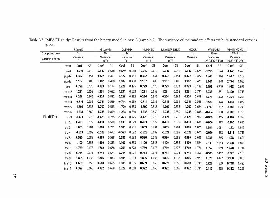
3.3R
esults
Table 3.5: IMPACT study: Results from the binary model in case 3 (sample 2). The variance of the random effects with its standard error isgiven
R(lme4) GLLAMM GLIMMIX NLMIXED MLwiN([R]IGLS) MIXOR WinBUGS MLwiN(MCMC) Computing time 1s 40s 1s 14s 1s 1s 75min 30min
Random Effects Variance: 0
Variance: 0(0)
Variance: 0( )
Variance: 0( )
Variance: 0(0)
Variance:
Variance: 28.040(22.130)
Variance: 19.892(17.236)
covar Coef SE Coef SE Coef SE Coef SE Coef SE Coef SE Coef SE Coef SE const -0.549 0.618 -0.549 0.618 -0.549 0.618 -0.549 0.618 -0.549 0.618 -0.549 0.674 -1.725 1.644 -1.448 1.473 pupil2 0.322 0.451 0.322 0.451 0.322 0.451 0.322 0.451 0.322 0.451 0.322 0.472 1.946 1.184 1.647 1.109 pupil3 1.187 0.408 1.187 0.408 1.187 0.408 1.187 0.408 1.187 0.408 1.187 0.471 3.141 1.148 2.774 1.085 age 0.729 0.175 0.729 0.174 0.729 0.175 0.729 0.175 0.729 0.174 0.729 0.189 2.195 0.719 1.913 0.675
motor2 1.231 0.653 1.231 0.652 1.231 0.653 1.231 0.653 1.231 0.652 1.231 0.791 3.933 1.851 3.400 1.713 motor3 0.226 0.562 0.226 0.562 0.226 0.562 0.226 0.562 0.226 0.562 0.226 0.608 1.571 1.332 1.304 1.231 motor4 -0.714 0.539 -0.714 0.539 -0.714 0.539 -0.714 0.539 -0.714 0.539 -0.714 0.569 -1.553 1.128 -1.434 1.062 motor5 -1.700 0.533 -1.700 0.533 -1.700 0.533 -1.700 0.533 -1.700 0.533 -1.700 0.624 -3.742 1.312 -3.382 1.243 motor6 -1.238 0.860 -1.238 0.859 -1.238 0.860 -1.238 0.860 -1.238 0.859 -1.238 0.898 -0.484 1.978 -0.800 1.790 motor9 -1.423 0.775 -1.423 0.775 -1.423 0.775 -1.423 0.775 -1.423 0.775 -1.423 0.917 -0.969 1.415 -1.107 1.333 trial2 0.433 0.579 0.433 0.579 0.433 0.579 0.433 0.579 0.433 0.579 0.433 0.606 -0.900 1.883 -0.600 1.650 trial3 1.083 0.781 1.083 0.781 1.083 0.781 1.083 0.781 1.083 0.781 1.083 1.021 1.381 2.091 1.292 1.847 trial4 -0.523 0.692 -0.523 0.692 -0.523 0.692 -0.523 0.692 -0.523 0.692 -0.523 0.671 -2.070 1.898 -1.813 1.715 trial5 0.580 0.588 0.580 0.588 0.580 0.588 0.580 0.588 0.580 0.588 0.580 0.606 1.936 1.845 1.598 1.601 trial6 1.100 0.853 1.100 0.853 1.100 0.853 1.100 0.853 1.100 0.853 1.100 1.524 2.633 2.053 2.398 1.876 trial7 1.769 0.678 1.769 0.678 1.769 0.678 1.769 0.678 1.769 0.678 1.769 1.776 1.657 1.919 1.678 1.744 trial8 0.714 0.671 0.714 0.671 0.714 0.671 0.714 0.671 0.714 0.671 0.714 1.356 -0.515 2.412 -0.226 2.135 trial9 1.805 1.033 1.805 1.033 1.805 1.033 1.805 1.033 1.805 1.033 1.805 0.923 4.520 3.447 3.968 3.005 trial10 0.689 0.655 0.689 0.655 0.689 0.655 0.689 0.655 0.689 0.655 0.689 0.745 0.727 1.579 0.748 1.425
Fixed Effects
trial11 0.322 0.668 0.322 0.668 0.322 0.668 0.322 0.668 0.322 0.668 0.322 0.741 0.412 1.405 0.382 1.296 37

Chapter 3 Logistic random effects ... and ordinal outcomes
3.3.4 Case 4: cross-classified binary logistic random effects model based on full data set
Only lme4 in R, GLIMMIX, MLwiN ([R]IGLS), WinBUGS, MLwiN (MCMC) and MCM-Cglmm could handle this analysis. The results for these packages were quite similar, asshown in Table 3.6. For example for age the estimates (SD) were 0.623 (0.028), 0.617 (0.028),0.623 (0.028), 0.624 (0.028), 0.624 (0.027) and 0.635 (0.028), for lme4, GLIMMIX, MLwiN([R]IGLS), WinBUGS, MLwiN (MCMC) and MCMCglmm, respectively. The variances forthe random effect of center were 0.116, 0.113, 0.116, 0.119, 0.120 and 0.106, respectively andfor the random effect of trial they were 0.067, 0.075, 0.067, 0.114, 0.095 and 0.094, respec-tively.
38
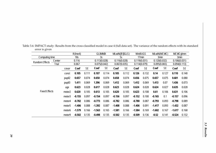
3.3R
esults
Table 3.6: IMPACT study: Results from the cross-classified model in case 4 (full data set). The variance of the random effects with its standarderror is given
R(lme4) GLIMMIX MLwiN([R]IGLS) WinBUGS MLwiN(MCMC) MCMCglmm Computing time 18s 3s 5s 17min 3min 3min
Center 0.116 0.113(0.028) 0.116(0.028) 0.119(0.031) 0.120(0.032) 0.106(0.031) Random Effects Trial 0.067 0.075(0.042) 0.067(0.035) 0.114(0.079) 0.095(0.065) 0.094(0.113) covar Coef SE Coef SE Coef SE Coef SE Coef SE Coef SE const 0.105 0.111 0.107 0.114 0.105 0.112 0.126 0.132 0.14 0.127 0.110 0.140 pupil2 0.657 0.074 0.650 0.074 0.658 0.074 0.656 0.075 0.657 0.075 0.681 0.080 pupil3 1.411 0.069 1.396 0.069 1.412 0.069 1.412 0.069 1.413 0.07 1.436 0.073 age 0.623 0.028 0.617 0.028 0.623 0.028 0.624 0.028 0.624 0.027 0.635 0.028
motor2 0.620 0.105 0.613 0.105 0.620 0.105 0.623 0.108 0.61 0.106 0.631 0.106 motor3 -0.155 0.097 -0.154 0.097 -0.156 0.097 -0.152 0.100 -0.165 0.1 -0.157 0.096 motor4 -0.782 0.086 -0.773 0.086 -0.782 0.086 -0.780 0.087 -0.793 0.093 -0.798 0.089 motor5 -1.406 0.088 -1.392 0.087 -1.408 0.088 -1.406 0.091 -1.417 0.093 -1.432 0.087 motor6 -1.579 0.166 -1.563 0.165 -1.581 0.166 -1.584 0.169 -1.602 0.167 -1.617 0.168
Fixed Effects
motor9 -0.502 0.135 -0.498 0.135 -0.502 0.135 -0.509 0.136 -0.52 0.141 -0.524 0.132
39
Chapter 3 Logistic random effects ... and ordinal outcomes
3.3.5 Cases 5 and 6: cross-classified binary logistic random effects models on samples 1and 2
As for case 2, we obtained in case 5 essentially the same results with all packages. For case6, the frequentist results were similar but the Bayesian results were different and were muchaffected by the prior of the variance parameter as in case 3 (tables for cases 5 and 6 are notshown).
3.3.6 Usability, flexibility and speed
The packages greatly differed in their usability, by which we mean the availability of diag-nostic tools/plots; ease of displaying/extracting parameter estimates and exporting results,etc. But it must be stated that all packages require a sound statistical knowledge in multi-level modelling in order to analyze such data in a reliable manner.SAS is based on procedures for which certain options can be turned on and off. Under-standing the different options in the statistical SAS procedures often requires a great dealof statistical background since the procedures are based on the most advanced and com-putationally powerful methods. Also SAS data management is quite powerful but is alsoassociated with a steep learning curve. The SAS procedures NLMIXED and MCMC offersome programming facilities.The package R has gained a lot of attention in the last decade and is becoming increasinglypopular among statisticians and non-statisticians. It requires programming skills and hasmany basic functions. In addition, R offers great graphics to the user. For the MCMCglmmpackage in R, we experienced difficulties in understanding the syntax for specifying theprior of the variance parameters as explained in the manual.Stata is very handy for analyzing simple as well as complicated problems. It has a command-line interface and also includes a graphical user interface since version 8.0. The softwareallows user-written packages just as in R and provides some programming facilities. Thepackage GLLAMM is powerful in dealing with a large range of complex problems.WinBUGS is the most popular general purpose package for Bayesian analysis with nowmore than 30,000 registered users. The package allows for a great variety of analyses usinga programming language that resembles to some extent that of R. WinBUGS requires aboutthe same programming skills as R.MIXOR needs no programming but provides very limited output. Furthermore, MLwiNhas a clear and intuitive interface to specify a random effects model, but lacks a simple syn-tax file structure.The packages also differ in what they offer as standard output besides the parameter esti-mates. WinBUGS allows for the most extensive output, including diagnostic plots for modelevaluation and plots of the individual random center effects. All packages except MIXORcan provide estimates of the random effects. In Figure 1 we show the box plots of the sam-pled random effects in WinBUGS for the first 10 centers of the binary logistic random effectsmodel applied to the IMPACT data. Of course with packages like SAS and R the output of
40

3.3 Results
the statistical procedures can be saved and then processed by some other procedure or func-tion to deliver the required graph or additional diagnostic analysis. For example, Figure 2is produced with R and shows the histogram of the random effects of the binary IMPACTlogistic random effects model.
Figure 3.1: IMPACT study: Box plot of a sample of the random effects (for center 1 to 10).Each box represents a center with its random effects estimate and confidenceinterval.
Flexibility differs somewhat in the packages. All packages could handle a probit modeland a log(-log) model except lme4 and MCMCglmm (MCMCglmm allows for logit or probitlink functions for a binary model but only the probit link function for the ordinal model).But, only WinBUGS allows for changing the distribution of the random effects. Table 1shows that WinBUGS has the greatest flexibility in adapting the model assumptions.
41

Chapter 3 Logistic random effects ... and ordinal outcomes
Figure 3.2: IMPACT study: Histogram of the random effects in the binary model in R
42
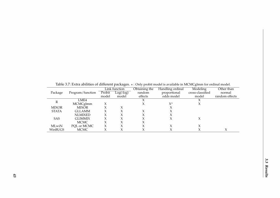
3.3R
esults
Table 3.7: Extra abilities of different packages. ? : Only probit model is available in MCMCglmm for ordinal model.
Package Program/functionLink function Obtaining the Handling ordinal Modeling Other than
Probit Log(-log) random proportional cross-classified normalmodel model effects odds model model random effects
R LME4 X XMCMCglmm X X X? X
MIXOR MIXOR X X XSTATA GLLAMM X X X X
SASNLMIXED X X X XGLIMMIX X X X X X
MCMC X X XMLwiN PQL or MCMC X X X X X
WinBUGS MCMC X X X X X X
43
Chapter 3 Logistic random effects ... and ordinal outcomes
The speed of the computations varied widely. All computations were done on an IntelCore(TM) 2 Duo E8400 processor with 3.0 GHz CPU and 3.21 GB internal memory. For case1, only a few seconds were needed to provide the estimates with the frequentist approachesto fit the binary logistic random effects, except for SAS NLMIXED and Stata GLLAMMwhich needed 15 minutes and 7 minutes, respectively. The MLwiN ([R]IGLS) procedure(using 2nd order PQL) was the fastest, and GLIMMIX was almost as fast followed by lme4and MIXOR. The Bayesian approaches were considerably slower, which is not surprisingsince MCMC sampling is time consuming. However, a major handicap to perform an hon-est comparison with regard computational speed is that the checking for convergence ofMCMC methods is far more difficult than in a frequentist sense (Gelman et al., 2003) andnot standardized. Nevertheless, MCMCglmm was the winner this time, but we consideredall computation times as acceptable, except for the SAS MCMC procedure which took 37hours for the binary model. Similar findings were obtained for the ordinal logistic randomeffects model, but compared to the binary model, the time to converge increased consider-ably for some software. Now the winner in the frequentist software was GLIMMIX closelyfollowed up by MIXOR. For the Bayesian software, MLwiN (MCMC) was the winner, muchfaster than WinBUGS. The SAS procedure MCMC never got to convergence (we stoppedit) and as mentioned above, the MCMCglmm program does not allow the ordinal logisticrandom effects model.
3.4 Discussion
3.4.1 Performance of each package
Although the parameter estimates were very similar between the ten software implementa-tions, we found considerable variations in computing time, usability and flexibility.Speed: Most of the frequentist approaches were very fast, taking only seconds, with theSAS NLMIXED procedure and the Stata package GLLAMM as exceptions. Overall, the SASprocedure GLIMMIX, the program MIXOR and the package MLwiN ([R]IGLS) were thewinners. The fact that NLMIXED and GLLAMM took much longer time has much to dowith that they are general purpose programs suitable for fitting a variety of complex ran-dom effects models and that they both use the AGQ method. The Bayesian approacheswere invariably slower than the frequentist approaches, which is due to the computationalintensive MCMC approach and that convergence is much harder to judge than in a classicalfrequentist sense. The speed of the Bayesian procedures appears to depend also more on thesample size than the frequentist approaches. As a result, long processing times as in Win-BUGS (14 minutes for binary and 8 hours for ordinal model, respectively) may prevent theuser to do much on exploratory statistical research. The R package MCMCglmm and ML-wiN (MCMC) were much faster than WinBUGS, taking only a few minutes for both binaryand ordinal cases. Hence, from a computational point of view, MCMCglmm and MLwiN(MCMC) are our software of choice for multilevel modeling.In our experience, the SAS procedure MCMC was inefficient in dealing with mixed models.
44

3.4 Discussion
It was far too time consuming (37 hours for the binary model) and it did converge neitherfor the regression coefficients nor for the variance of the random effects. At this moment, wecannot recommend this SAS procedure for fitting logistic random effects regression models.Usability and flexibility: The packages differ much in nature, like working interface anddata management. MLwiN and MIXOR are menu-driven although writing syntax is alsoallowed in both packages. SAS is supposed to work in batch mode with some proceduresand macros. The others, WinBUGS, R and STATA, are embedded in a programming lan-guage. Which package to prefer from the usability viewpoint is difficult to say since it verymuch depends on the user but also on whether the logistic random effects model fitting isa stand-alone exercise. We know that in practice this is often not the case since we wouldlike to process output of such an analysis to produce e.g. nice graphs. From this viewpointMIXOR and WinBUGS score lower since they require the user to switch to other software,such as R, to produce additional output or better quality graphs. However, in recent yearssome packages, like R2WinBUGS in R, can combine WinBUGS and R (or other software)nicely. See the BUGS website (The BUGS project, nd) to get more information.For the cross-classified random effects model and the sub-dataset analysis, some integrationmethods and optimization techniques were not available in some software. For example, inGLIMMIX, AGQ is not available for the cross-classified random effects model and we hadto change to Residual Subject-specific Pseudo-Likelihood.In the R package MCMCglmm, by default the residual variance should be explicitly spec-ified for random effects models. But, as this variance parameter is not identifiable for thelogistic random effects model, as seen above, it has to be fixed at a particular value. MCM-Cglmm uses arbitrary values larger than zero, while the other packages ignore the residualvariance since it does not play a role in the estimation process. In order to make the resultscomparable, the posteriors had to be rescaled which worked most often. But one should beaware that the prior specification will be different after rescaling the posteriors, so there willbe differences between MCMCglmm and other Bayesian packages if the prior considerablyinfluences the posterior which happened here for cases 3 and 6.RIGLS is the restricted version of IGLS in a similar way as REML is a restricted maximumlikelihood procedure, with RIGLS less biased especially in linear models, as mentioned be-fore. In logistic random effects models, IGLS was chosen for MLwiN ([R]IGLS) in our studyas all other frequentist packages allow for the ML method but not all allow for REML esti-mation. An additional MLwiN analysis using RIGLS did show somewhat different results.For case 1, the results from RIGLS and IGLS were basically identical, only the varianceestimator was 10% higher with RIGLS. For case 3, the regression estimates differed moreand the RIGLS estimator of variance was not zero anymore. For more information on ML,REML, etc in different multilevel models, see Browne and Draper (2006).WinBUGS demonstrates much flexibility. Different distributions for the random effects (e.g.gamma, uniform, t-distribution) and different link functions such as probit and log(-log)model are possible. Different link functions are also possible in the SAS procedures GLIM-MIX and NLMIXED, but none of these two packages allow for other than normal distribu-tions for the random effects. Note that in our study the binary logistic random effects model
45
Chapter 3 Logistic random effects ... and ordinal outcomes
was superior to the probit and log(-log) models according to Akaike Information Criterion(using GLIMMIX).
3.4.2 Problems with small data sets
When the data set is small and the variance of the random effects is near zero, or the ICC(intra-class correlation) is very small as in cases 3 and 6, both frequentist and Bayesian meth-ods can give quite different estimates especially for the variance. The MLE approach mighthave difficulties estimating small but non-zero variance estimates. The variance was esti-mated zero with lme4 in R. GLLAMM also estimated the variance as well as its standarderror as quite small. GLIMMIX and NLMIXED produced very small estimates for the vari-ance but no output for the standard error. MLwiN ([R]IGLS) estimated the variance andthe standard error as zero. Finally, MIXOR gave no output for either the variance or thestandard error.For the Bayesian methods, the posterior means depended much on the choice of prior forthe variance component. In order to check their impact, we offered WinBUGS the fol-lowing three priors for the standard deviation of the random effects: uniform (0,1), uni-form (0,10), uniform (0,100), and a uniform (0, 106) as well as an inverse Gamma distribu-tion (0.001,0.001) for the variance. We also offered two priors for the variance in MLwiN(MCMC): inverse Gamma distribution (0.001,0.001) and uniform (0, ). This uniform distri-bution is actually an improper prior which might lead to an improper posterior. Further,it is not the default choice in MLwiN. However, when the default procedure was takenfor the improper uniform prior, i.e. starting values are taken from an initial IGLS run, thestarting value for the variance parameter was taken too small and remained so until theMCMC sampling was stopped thereby affecting severely all parameters. For this reasonwe restarted this MLwiN run with 1 as the starting value which solved this problem. Thetotal number of iterations was 1,100,000 with a burn-in of 100,000 iterations with thinningapplied every 10 iterations. Convergence was checked and obtained using the criteria of-fered in each software package. The results are shown in Table 3.8. We can see that mostof the Bayesian estimates are larger than the frequentist MLE from Table 3.5, especially forthe variance parameter. The reason is that the posterior distribution is highly skewed forthe variance therefore the posterior mean is much larger than the posterior mode whosefrequentist counterpart is the MLE. We also notice in Table 3.8 that the variance estimates inMLwiN and WinBUGS using a uniform prior on the variance are greater than the WinBUGSresults with uniform priors on the standard deviation, which was mentioned by Gelman(2006). To conclude, for small data sets the choice of the prior matters for the posterior esti-mates of the parameters, as was also shown by e.g. Spiegelhalter et al. (2004).
46

3.4D
iscussion
Table 3.8: Impact of variance component priors on the posterior means in WinBUGS and MLwiN in case 3 (sample 2). The variance of therandom effects with its standard error is given. The first three uniform distributions in WinBUGS are for the standard deviation ofthe random effects and the rest four prior distributions are for the variance of the random effect
WinBUGS MLwiN (MCMC) Distribution Uniform(0,1) Uniform(0,10) Uniform(0,100) Uniform(0,106) IG (0.001,0.001) IG (0.001,0.001) Uniform(0,infinity)
Random Effects Variance: 0.489(0.312)
Variance: 26.450(18.250)
Variance: 28.040(22.130)
Variance: 36.950(29.120)
Variance: 20.310(17.570))
Variance: 19.892(17.236)
Variance: 36.954(28.406)
covar Coef SE Coef SE Coef SE Coef SE Coef SE Coef SE Coef SE const -0.599 0.695 -1.720 1.610 -1.725 1.644 -1.942 1.830 -1.463 1.482 -1.448 1.473 -1.970 1.833 pupil2 0.435 0.510 1.927 1.161 1.946 1.184 2.177 1.267 1.662 1.121 1.647 1.109 2.198 1.270 pupil3 1.384 0.461 3.098 1.101 3.141 1.148 3.455 1.236 2.789 1.093 2.774 1.085 3.457 1.224 age 0.869 0.199 2.160 0.679 2.195 0.719 2.428 0.781 1.928 0.686 1.913 0.675 2.437 0.777
motor2 1.484 0.737 3.897 1.799 3.933 1.851 4.384 2.008 3.436 1.728 3.400 1.713 4.396 2.017 motor3 0.319 0.630 1.557 1.310 1.571 1.332 1.777 1.433 1.328 1.243 1.304 1.231 1.785 1.431 motor4 -0.838 0.602 -1.526 1.121 -1.553 1.128 -1.627 1.205 -1.445 1.052 -1.434 1.062 -1.637 1.205 motor5 -1.953 0.594 -3.685 1.277 -3.742 1.312 -4.026 1.407 -3.406 1.237 -3.382 1.243 -4.032 1.400 motor6 -1.473 0.986 -0.519 1.931 -0.484 1.978 -0.158 2.143 -0.784 1.795 -0.800 1.790 -0.161 2.131 motor9 -1.561 0.868 -0.974 1.404 -0.969 1.415 -0.852 1.495 -1.099 1.328 -1.107 1.333 -0.851 1.486 trial2 0.391 0.659 -0.846 1.823 -0.900 1.883 -1.248 2.120 -0.612 1.672 -0.600 1.650 -1.212 2.115 trial3 1.131 0.888 1.362 2.033 1.381 2.091 1.407 2.299 1.298 1.854 1.292 1.847 1.415 2.321 trial4 -0.682 0.781 -2.034 1.860 -2.070 1.898 -2.312 2.080 -1.809 1.722 -1.813 1.715 -2.286 2.085 trial5 0.639 0.667 1.913 1.792 1.936 1.845 2.219 2.100 1.614 1.636 1.598 1.601 2.242 2.078 trial6 1.318 0.975 2.640 2.019 2.633 2.053 2.781 2.193 2.428 1.893 2.398 1.876 2.786 2.200 trial7 1.889 0.822 1.663 1.906 1.657 1.919 1.603 2.087 1.696 1.753 1.678 1.744 1.631 2.072 trial8 0.698 0.818 -0.469 2.338 -0.515 2.412 -0.869 2.692 -0.242 2.142 -0.226 2.135 -0.811 2.679 trial9 2.084 1.190 4.445 3.357 4.520 3.447 4.956 3.877 3.994 3.052 3.968 3.005 4.988 3.888 trial10 0.744 0.742 0.742 1.560 0.727 1.579 0.665 1.693 0.742 1.439 0.748 1.425 0.670 1.693
Fixed Effects
trial11 0.311 0.747 0.422 1.394 0.412 1.405 0.417 1.496 0.389 1.298 0.382 1.296 0.421 1.496
47

Chapter 3 Logistic random effects ... and ordinal outcomes
3.4.3 Comparison with previous studies
Zhou et al (1999) compared 5 packages for generalized linear multilevel models. They com-pared the estimates, the computing time and the features of the packages. In our study, wecompared 10 (popular) packages on similar features. Also Bayesian methods were included.Guo and Zhao (2000) compared statistical software for multilevel modelling of binary data,and they put much emphasis on PQL and MQL. Furthermore, the SAS macro GLIMMIX aswell as MLn, the DOS predecessor of MLwiN, were included in their comparison. The latterpackages are not in use anymore which makes this comparison now outdated.The CMM website published an online report (multilevel modelling software reviews) whichcompared almost 20 packages for the normal linear model, the binary response model, theordered category model and the cross-classified model (The center for multilevel modeling(CMM) website, nd). But the packages lme4, MCMCglmm and the SAS procedures GLIM-MIX and MCMC were not considered in this review. In addition, we evaluated here also theusability and flexibility of the packages.
3.5 Conclusions
We conclude from our study that for relatively large data sets, the parameter estimatesfrom logistic random effects regression models will probably not be much influenced bythe choice of the statistical package. In that case the choice of the statistical implementationshould depend on other factors, such as speed and desired flexibility. Based on our study,we conclude that if there is no prior acquaintance with a certain package and preference isgiven to a frequentist approach, the following packages are to be recommended: MLwiN([R]IGLS), the R package lme4 and the SAS procedure GLIMMIX. For a Bayesian imple-mentation, we would recommend MLwiN (MCMC) because of its efficiency. If the useris also interested in (perhaps more complicated) statistical analyses other than multilevelmodelling then he/she could choose WinBUGS.Finally, a cautionary remark is necessary, i.e. a ”large data set” can still be sparse and hence”large” should be interpreted with some caution. For example, a large data set with manylowest-level units nested within nearly as many higher-level units will act as a ”small” dataset when a multilevel model is fit. For such data sets the result of the fitting exercise mightvery much depend on the chosen approach: frequentist or Bayesian. In case a Bayesianpackage is chosen, the parameter estimates might be much influenced by the priors for thevariance of the random effects. Since some packages offer only a quite restricted set of priors(such as MLwiN) for this parameter, the choice of the Bayesian package may have a largeimpact on the posterior estimates of all parameters for ”small” data sets. Finally, also theperformance of a Bayesian analysis might very much depend on the chosen starting valuefor the variance parameter, e.g. when chosen (close to) zero the MCMC might be stuckaround zero for a very long time (which happened with MLwiN) and thus affect severelythe convergence of the Markov chain.
48

References
References
Austi, P. C., Alte, D. A., et al. (2003). Comparing hierarchical modeling with traditionallogistic regression analysis among patients hospitalized with acute myocardial infarction:should we be analyzing cardiovascular outcomes data differently? American Heart Journal,145(1):27–35.
Bates, D., Maechler, M., and Ben, B. (2009). Package lme4.
Brooks, S. P. and Gelman, A. (1998). General methods for monitoring convergence of iter-ative simulations. Journal of Computational and Graphical Statistics, 7(4):434–455.
Browne, W. J. and Draper, D. (2006). A comparison of bayesian and likelihood-based meth-ods for fitting multilevel models. Bayesian Analysis, 1(3):473–514.
Browne, W. J. and Rasbash, J. (2009). MCMC estimation in MLwiN.
Gelman, A. (2006). Prior distributions for variance parameters in hierarchical models (com-ment on article by Browne and Draper). Bayesian Aanalysis, 1(3):515–534.
Gelman, A., Carlin, J. B., Stern, H. S., and Rubin, D. B. (2003). Bayesian Data Analysis,Second Edition (Chapman & Hall/CRC Texts in Statistical Science). Chapman and Hall/CRC,2 edition.
Goldstein, H. (1989). Restricted unbiased iterative generalized least-squares estimation.Biometrika, 76(3):622–623.
Goldstein, H. (2011). Multilevel Statistical Models, volume 922. Wiley.
Guo, G. and Zhao, H. (2000). Multilevel modeling for binary data. Annual Review of Sociol-ogy, 26:441–462.
Hadfield, J. D. (2010). MCMC methods for multi-response generalized linear mixed mod-els: the MCMCglmm R package. Journal of Statistical Software, 33(2):1–22.
Hedeker, D. and Gibbons, R. D. (1996). MIXOR: A computer program for mixed-effectsordinal regression analysis. Computer Methods and Programs in Biomedicine, 49(2):157–176.
Lesaffre, E. and Spiessens, B. (2001). On the effect of the number of quadrature points ina logistic random effects model: an example. Journal of the Royal Statistical Society: Series C(Applied Statistics), 50(3):325–335.
Lin, X. and Breslow, N. E. (1996). Bias correction in generalized linear mixed modelswith multiple components of dispersion. Journal of the American Statistical Association,91(435):1007–1016.
Maas, A. I., Marmarou, A., Murray, G. D., Teasdale, S. G. M., and Steyerberg, E. W. (2007).Prognosis and clinical trial design in traumatic brain injury: The impact study. Journal ofNeurotrauma, 24(2):232–238.
Marmarou, A., Lu, J., Butcher, I., McHugh, G. S., Mushkudiani, N. A., Murray, G. D.,Steyerberg, E. W., and Maas, A. I. (2007). IMPACT database of traumatic brain injury:Design and description. Journal of Neurotrauma, 24(2):239–250.
McHugh, G. S., Butcher, I., Steyerberg, E. W., Lu, J., Mushkudiani, N., Marmarou, A., Maas,A. I., and Murray, G. D. (2007). Statistical approaches to the univariate prognostic analysisof the IMPACT database on traumatic brain injury. Journal of Neurotrauma, 24(2):251–258.
Molenberghs, G. and Verbeke, G. (2005). Models for discrete longitudinal data. Springer.
Ng, E. S., Carpenter, J. R., Goldstein, H., and Rasbash, J. (2006). Estimation in generalisedlinear mixed models with binary outcomes by simulated maximum likelihood. StatisticalModelling, 6(1):23–42.
49
Chapter 3 Logistic random effects ... and ordinal outcomes
Pendergast, J. F., Gange, S. J., Newton, M. A., Lindstrom, M. J., Palta, M., and Fisher, M. R.(1996). A survey of methods for analyzing clustered binary response data. InternationalStatistical Review/Revue Internationale de Statistique, 64(1):89–118.
Rabe-Hesketh, S., Skrondal, A., and Pickles, A. (2004). GLLAMM manual.
Rasbash, J. (n.d.). What are multilevel models and why should I use them?[http://www.cmm.bristol.ac.uk/learning-training/multilevel-models/what-why.shtml].
Rasbash, J., Browne, W., Goldstein, H., Yang, M., Plewis, I., Healy, M., Woodhouse, G.,Draper, D., Langford, I., and Lewis, T. (2000). A User’s Guide to MLwiN.
Rodrıguez, G. and Elo, I. (2003). Intra-class correlation in random-effects models for binarydata. The Stata Journal, 3(1):32–46.
Rodriguez, G. and Goldman, N. (1995). An assessment of estimation procedures for multi-level models with binary responses. Journal of the Royal Statistical Society. Series A (Statisticsin Society), 158(1):73–89.
Snijders, T. A. and Bosker, R. J. (2011). Multilevel analysis: An introduction to basic and ad-vanced multilevel modeling. Sage Publications Limited.
Spiegelhalter, D. J., Abrams, K. R., and Myles, J. P. (2004). Bayesian approaches to clinicaltrials and health-care evaluation. John Wiley & Sons.
Steyerberg, E. W., Mushkudiani, N., Perel, P., Butcher, I., Lu, J., McHugh, G. S., Murray,G. D., Marmarou, A., Roberts, I., Habbema, J. D. F., et al. (2008). Predicting outcome af-ter traumatic brain injury: development and international validation of prognostic scoresbased on admission characteristics. PLoS Medicine, 5(8):e165.
The BUGS project (n.d.). Calling WinBUGS 1.4 from other programs. [http://www.mrc-bsu.cam.ac.uk/bugs/winbugs/remote14.shtml].
The center for multilevel modeling (CMM) website (n.d.). Comparative timings.[http://www.cmm.bristol.ac.uk/learning-training/multilevel-m-software/tables.shtml].
The GLIMMIX procedure (2009). SAS/STAT Users Guide. Version 9.2.
The MCMC procedure (2009). SAS/STAT Users Guide. Version 9.2.
The NLMIXED procedure (2009). SAS/STAT Users Guide. Version 9.2.
Zhou, X.-H., Perkins, A. J., and Hui, S. L. (1999). Comparisons of software packages forgeneralized linear multilevel models. The American Statistician, 53(3):282–290.
50
4A MULTI-COUNTRY PERSPECTIVE ON
NURSES TASKS BELOW THEIR SKILLLEVEL: REPORTS FROM DOMESTICALLY
TRAINED NURSES AND FOREIGNTRAINED NURSES FROM DEVELOPING
COUNTRIES
Chapter 4 is based on the paper:Bruyneel, L., Li, B., Squires, A., Aiken, L., Lesaffre, E., Van den Heede, K., and Sermeus, W. (2013).A multi-country perspective on nurses tasks below their skill level: Reports from domestically trainednurses and foreign trained nurses from developing countries. International Journal of Nursing Stud-ies, 50(2):202-209.
51
Chapter 4 A multi-country ... from developing countries
Abstract
Several studies have concluded that the use of nurses time and energy isoften not optimized. Given widespread migration of nurses from devel-oping to developed countries, it is important for human resource plan-ning to know whether nursing education in developing countries is as-sociated with more exaggerated patterns of inefficiency. In this paper weaim to describe nurses reports on tasks below their skill level as well as toexamine the association between nurses migratory status (domesticallytrained nurse or foreign trained nurse from a developing country) andreports on these tasks. The data set for the Registered Nurse ForecastingStudy was used which was a cross-sectional study having 33,731 nursesin 486 hospitals in twelve European counties. Logistic random effectsmodels were applied to estimate the effect of nurses migratory statuson reports of the tasks below their skill level they performed. The find-ings suggest that there remains much room for improvement to optimizethe use of nurses time and energy. Special attention should be given toraising the professional level of practice of foreign trained nurses fromdeveloping countries. Further research is needed to understand the in-fluence of professional practice standards, skill levels of foreign trainednurses from developing countries and values attached to these tasks re-sulting from previous work experiences in their home countries. Thiswill allow us to better understand the conditions under which foreigntrained nurses from developing countries can optimally contribute toprofessional nursing practice in developed country contexts.
52
4.1 Background
4.1 Background
System-level interventions like increasing nurse staffing and creating superior work envi-ronments have been associated with improved patient safety outcomes and a higher degreeof nurse wellbeing (Aiken et al., 2012; Kelly et al., 2012). Also central to the efficient structur-ing of nurses work is optimizing the use of their time and effort. When asked about their lastshift however, nurses across three countries (US, Canada, Germany) consistently reportedhigh percentages of non-nursing tasks performed, including transporting of patients, deliv-ering or retrieving of food trays, and performing of housekeeping activities. At the sametime, they reported many nursing tasks that were necessary but left undone because theylacked the time to complete them (Aiken et al., 2001). Al-Kandari and Thomas (2009) usedthe list of non-nursing tasks from the study of Aiken and colleagues among 780 Kuwaitinurses. Increased non-nursing task workload was positively correlated to incompletionof nursing activities. Two recent time-and-motion studies found that nurses spent con-siderable amounts of time in non-nursing activities. A 36-hospital time-and-motion studyfound that activities considered by nurses to be waste (waiting, looking, retrieving, and de-livering) consumed 6.6% of reported time per 10-h shift (Hendrich et al., 2008). Anothertime-and-motion study showed that nurses spent 9.0% of their time during their last shifton non-nursing tasks, including replenishing charts and forms, tidying up rooms, makingbeds, answering phones, searching for people, gathering linen, and answering call bells(Desjardins et al., 2008).
The employment of internationally trained nurses may suggest a shortage of nurses at theinstitution or national level. Thus it is particularly important to optimize the full scope ofprofessional nursing practice in institutions that employ nurses educated in other countries.Studies have shown that migrant nurses sometimes experience discrimination by means oflower wage and less upward mobility, and may be employed as nursing aids rather thanas nurses, which negatively impacts their wellbeing (Kline, 2003; Center for Health Work-force Studies, 2008; Organisation for Economic Cooperation and Development, 2010). Otherresearch suggests that nurses trained abroad aspire to the same professional nursing prac-tice standards common to their country of current employment (Flynn and Aiken, 2002).In light of the increasing international mobility of nurses, Humphries et al. (2009) finds theevaluation of how migrant nurses skills are utilized a prerequisite to incorporating nursemigration into workforce planning.
The twelve-country Registered Nurse Forecasting (RN4CAST) study measured and linkedorganizational features of nurses work places to nurse wellbeing and patient outcomes tochallenge assumptions underpinning previous nurse workforce planning efforts (Sermeuset al., 2011). The aim of this study is to determine whether there is a difference between do-mestically trained and foreign trained nurses from developing countries in nurses reportson tasks below their skill level performed during their last shift. We consider the implica-tions of our findings for human resources management.
53

Chapter 4 A multi-country ... from developing countries
4.2 Methods
Study design
The RN4CAST study favoured a rigorous quantitative multi-country cross-sectional designon the basis of research methods used in a five-nation study of critical issues in nurse staffingand the impact on patient care (Aiken et al., 2001). Data were gathered via four data sources(nurse, patient and hospital profile surveys and routinely collected hospital discharge data).The design of the RN4CAST-study is described in detail by Sermeus et al. (2011). For thisanalysis, nurse-reported information on migratory status and tasks below skill level per-formed during their last shift was used.
Ethical approval
Depending on national legislation, the study protocol was approved by either central ethicalcommittees (e.g. nation or university) or local ethical committees (e.g. hospitals). All nursesreceived an information letter explaining the design of the study.
Study sample
A total of 486 hospitals were sampled as primary sampling units in twelve European coun-tries, with at least 30 hospitals per country. In two countries, the selected hospitals representall of the relevant institutions in the country (Ireland, Norway). In Belgium, Germany, theNetherlands, Switzerland, England and Spain, a stratified random selection (geographicallocation within the countries, hospital size, and hospital type) was done. Additionally, theBelgian and German research teams also gave the opportunity for hospitals to participateon a voluntary basis. In Finland, Poland and Greece, hospitals were selected via purposivesampling (i.e. geographical spread, hospital size, hospital type). In Sweden, all nurses wereapproached via the Swedish Nursing Association, which covers about 85% of all nursesworking in Sweden. Nurses were then asked to identify the hospital in which they work.
In each of the selected hospitals at least two general medical and surgical nursing unitswere randomly selected from a master list of nursing units. All staff nurses involved indirect patient care activities served as informants on organization of nursing care, nursewellbeing, patient safety and quality of care. Nurses were defined in each country as thosemeeting the European Union definition of trained and licensed nurses according to directive2005/35/EC. The sample consists of 33,731 nurses (62% response rate) from Belgium (n =3186), England (n = 2990), Finland (n = 1131), Germany (n = 1508), Greece (n = 367), Ireland(n = 1406), the Netherlands (n = 2217), Norway (n = 3752), Poland (n = 2605), Spain (n =2804), Sweden (n = 10,133), and Switzerland (n = 1632).
Study measures
A self-administered questionnaire was distributed. Nurses were asked to indicate whetherthey had received their training in the country they are currently working in and if not, in
54
4.2 Methods
which country they did receive their training. Based on the World Economic Outlook clas-sification of countries (International Monetary Fund, 2010), nurses were categorized intodomestically trained, foreign trained in a country with an emerging or developing econ-omy (further referred to as foreign trained in a developing country), or foreign trained in acountry with an advanced economy (further referred to as foreign trained in a developedcountry). The IMF list of emerging and developing economies (150 out of 184 countries)includes countries from all over the world. Some recent entrants to the European Union forexample have remained classified as emerging economies (e.g. Latvia, Poland).
Within a series of questions about their last shift, nurses were asked to report on a listof tasks below their skill level whether they had performed these tasks never, sometimes,or often during their last shift. The following nine tasks were presented to nurses: rou-tine phlebotomy/blood draw for tests, transporting of patients within hospitals, perform-ing non-nursing care, performing non-nursing services not available on off-hours, deliver-ing and retrieving food trays, answering phones/clerical duties, arranging discharge refer-rals and transportation, obtaining supplies or equipment, and cleaning patient rooms andequipment.
Three types of variables were used to control for confounders: nurses type of last shiftworked (morning, evening, night), number of years worked as a nurse and level of educa-tion (bachelor degree or not).
Statistical analysis
We first described for each country the share of foreign trained nurses and the share ofnurses from developing and developed countries. We provide detailed data on the coun-try of origin. We also assess whether there are statistically significant differences betweendomestically trained nurses and foreign trained nurses from developing countries in re-porting type of last shift worked, number of years worked, and level of education. Sec-ond, we described nurses reports on the list of nine tasks performed during their last shift.Third, we compared reports on tasks performed by domestically trained nurses and foreigntrained nurses from developing countries. For analytic purposes, we dichotomized nursesresponses as never performed and sometimes/often performed. A heat map (Sneath, 1957)was used to graphically compare these reports, with a system of colour-coding where a darkgrey square indicates that a higher proportion of foreign trained nurses from developingcountries reported this task compared to domestically trained nurses (and light grey squarevice versa). A composite measure of tasks performed during nurses last shift (min = 0, max= 9) was calculated for each individual nurse by taking the sum of the nine dichotomizednursing tasks. This composite measure had a binomial distribution. The overall effect (i.e.over all countries) of nurses migratory status on this composite measure was estimated us-ing a two-level logistic random effects regression. The country effect was modelled as afixed effect. The hospitals were treated as a random effect. We calculated the intraclasscorrelation coefficient at the hospital level as an indication of the degree of homogeneity.The analysis was adjusted for nurses type of last shift worked, number of years worked asa nurse and level of education. We analyzed the consistency of the overall effect by speci-
55

Chapter 4 A multi-country ... from developing countries
fying interaction effects between the countries under study and migratory status. We alsoconstructed a series of similar two-level random effects regression models to analyze theoverall effect of migratory status on each task separately. Despite all efforts to get randomeffects models with interaction effects to converge, this proved to be hard for four out ofnine tasks because of computational problems. Descriptive findings for these tasks showedrepetitive high proportions of both domestically trained nurses and foreign trained nursesfrom developing countries indicating they had performed these tasks during their last shift.We repeated our analysis comparing nurses reports on tasks never/sometimes performedand often performed, and found similar findings. We also compared the difference in tasksreported between domestically trained nurses and foreign trained nurses from a developedcountry and found no statistically significant differences. The data analysis for this pa-per was generated using SAS/STAT software, Version 9.3 of the SAS System for Windows.Copyright 2011 SAS Institute Inc. SAS and all other SAS Institute Inc. product or servicenames are registered trademarks or trademarks of SAS Institute Inc., Cary, NC, USA.
4.3 Findings
Foreign trained nurses
2107 nurses (6.2% of total sample) indicated they were trained in another country thanwhere they were currently employed, of which 832 were trained in a developing country(2.5% of total sample). There was large variation in the share of foreign trained nurses be-tween countries: Ireland (38.6%), Switzerland (22.1%) and England (16.7%), Norway (5.5%),Germany (5.1%), Greece (5.1%), Belgium (3.1%), Netherlands (2.4%), Sweden (2.3%), Spain(1.3%), Finland (.9%). In Poland, all nurses that participated in the study were domesti-cally trained nurses and in Greece there were no foreign trained nurses from developingcountries. The share of foreign trained nurses varied considerably between hospitals in thetop three countries with foreign trained nurses, ranging from 16% to 56% (Ireland), 4% to50% (Switzerland) and 1% to 52% (England). Countries with low numbers of foreign trainednurses from developing countries (Finland, Greece, Poland) or high missing values on coun-try of training (Belgium) were dropped for further analysis, which resulted in a total of 813foreign trained nurses from developing countries remaining for further analysis. Figure 4.1presents the large variation in the share of nurses from developing countries employed inthe sample of eight remaining European countries. While in Switzerland only 11% of theshare of foreign trained nurses were trained in developing countries, this ran up as highas 80% in England. In many countries, a large part of the share of foreign trained nursescould be explained by mobility between neighboring countries or countries in the region.31.6% (n = 112) of the foreign-trained nurses in Switzerland were trained in Germany, 30%(n = 107) were trained in France, and 12% (n = 41) were trained in Italy. Nurses trained indeveloping countries now working in Switzerland included nurses from India (2.0%, n = 7),Bahrain (1.4%, n = 4), the Philippines (1.1%, n = 3) and Bosnia and Herzegovina (.85%, n =3), among others. In Sweden 26.8% (n = 62) of the foreign trained nurses had obtained theirtraining in Finland, and 11.7% (n = 27) in Germany. The share of foreign trained nurses from
56
4.3 Findings
developing countries was ethnically very diverse, with most nurses trained in Bosnia andHerzegovina (6.5%, n = 15). In Spain a different image emerged, with a large share of nursestrained in South- American countries, mainly in Peru (21.6%, n = 8). Norways largest shareof the foreign trained nurse workforce was composed of 26.1% (n = 53) nurses trained inSweden, 15.3% (n = 31) in Australia, and 15.3% (n = 31) in Denmark. Like in Switzerland,nurses from developing countries came from the Philippines (2.5%, n = 5), Bahrain (1.5%, n= 3) and Bosnia and Herzegovina (1.5%, n = 3). In the Netherlands, next to Belgian (12.9%,n = 7) and German (9.3%, n = 5) nurses, there was a substantial percentage of nurses fromthe former Dutch colonies of Suriname (22.2%, n = 12) and Indonesia (14.1%, n = 8). Polish-trained nurses accounted for 17.1% (n = 13) of the German foreign trained nurse workforce,and Kazakh nurses accounted for 5.3% (n = 4). In England, the main source countries werethe Philippines (31.0%, n = 153) and India (22.7%, n = 117) but also nurses from sub-SaharanAfrica (Ghana, Kenia, Nigeria, South Africa, Uganda, Zambia and Zimbabwe) accountedfor a large proportion (15.9%, n = 78). Like in England, the use of overseas recruiters iswidespread in Ireland. Contrary to England however, Irelands share of nurses from de-veloping countries was almost completely accounted for by nurses from India (20.9%, n =111) and the Philippines (17.3%, n = 92) only. The share of European foreign trained nursesin Ireland (54.5% of total) was almost exclusively made up of nurses having received theirtraining in the UK (51.5% of total).
In all eight countries, foreign trained nurses from developing countries had more yearsof experience in working as a nurse. These differences were statistically significant acrossall countries. Statistically significant differences were found for the level of education inEngland and Ireland, where the share of foreign trained nurses from developing countriesreporting they had obtained a bachelor level degree in their home country was higher thanthe share of domestically trained nurses.
Nurses reports on tasks performed during their last shift
Across countries, a high proportion of nurses reported having sometimes or often per-formed tasks below their skill level during their last shift. Most reported tasks (country-weighted average) were answering phones/clerical duties (97.4%), performing non-nursingcare (90.1%), and obtaining supplies or equipment (71.2%). There was large variabilitybetween countries in nurses reports. For example in Spain, only 16.8% reported havingcleaned patient rooms and equipment, while in England this was 90% (see Table 4.1).
Comparison of reports from domestically trained nurses and nurses trained indeveloping countries
The heat map shows that in 62 out of 72 cases, higher percentages of nurses from develop-ing countries reported they performed these nine tasks, compared to domestically trainednurses (Table 4.1 for detailed findings). Findings were consistent between hospitals and inthe case of nurses from the same developing country working in different countries understudy here. For example, 25 English trusts had a total of 153 Philippines employed. In 24
57

Chapter 4 A multi-country ... from developing countries
country (2.5% of total sample). There was large variation inthe share of foreign trained nurses between countries:Ireland (38.6%), Switzerland (22.1%) and England (16.7%),Norway (5.5%), Germany (5.1%), Greece (5.1%), Belgium(3.1%), Netherlands (2.4%), Sweden (2.3%), Spain (1.3%),Finland (.9%). In Poland, all nurses that participated in thestudy were domestically trained nurses and in Greecethere were no foreign trained nurses from developingcountries. The share of foreign trained nurses variedconsiderably between hospitals in the top three countrieswith foreign trained nurses, ranging from 16% to 56%(Ireland), 4% to 50% (Switzerland) and 1% to 52% (England).Countries with low numbers of foreign trained nurses fromdeveloping countries (Finland, Greece, Poland) or highmissing values on country of training (Belgium) weredropped for further analysis, which resulted in a total of813 foreign trained nurses from developing countriesremaining for further analysis. Fig. 1 presents the largevariation in the share of nurses from developing countriesemployed in the sample of eight remaining Europeancountries. While in Switzerland only 11% of the share offoreign trained nurses were trained in developing coun-tries, this ran up as high as 80% in England. In manycountries, a large part of the share of foreign trained nursescould be explained by mobility between neighbouringcountries or countries in the region. 31.6% (n = 112) of theforeign-trained nurses in Switzerland were trained inGermany, 30% (n = 107) were trained in France, and 12%(n = 41) were trained in Italy. Nurses trained in developingcountries now working in Switzerland included nursesfrom India (2.0%, n = 7), Bahrain (1.4%, n = 4), the Philip-pines (1.1%, n = 3) and Bosnia and Herzegovina (.85%, n = 3),among others. In Sweden 26.8% (n = 62) of the foreigntrained nurses had obtained their training in Finland, and11.7% (n = 27) in Germany. The share of foreign trainednurses from developing countries was ethnicallyvery diverse, with most nurses trained in Bosnia and
Herzegovina (6.5%, n = 15). In Spain a different imageemerged, with a large share of nurses trained in South-American countries, mainly in Peru (21.6%, n = 8). Norway’slargest share of the foreign trained nurse workforce wascomposed of 26.1% (n = 53) nurses trained in Sweden,15.3% (n = 31) in Australia, and 15.3% (n = 31) in Denmark.Like in Switzerland, nurses from developing countriescame from the Philippines (2.5%, n = 5), Bahrain (1.5%,n = 3) and Bosnia and Herzegovina (1.5%, n = 3). In theNetherlands, next to Belgian (12.9%, n = 7) and German(9.3%, n = 5) nurses, there was a substantial percentage ofnurses from the former Dutch colonies of Suriname (22.2%,n = 12) and Indonesia (14.1%, n = 8). Polish-trained nursesaccounted for 17.1% (n = 13) of the German foreign trainednurse workforce, and Kazakh nurses accounted for 5.3%(n = 4). In England, the main source countries were thePhilippines (31.0%, n = 153) and India (22.7%, n = 117) butalso nurses from sub-Saharan Africa (Ghana, Kenia,Nigeria, South Africa, Uganda, Zambia and Zimbabwe)accounted for a large proportion (15.9%, n = 78). Like inEngland, the use of overseas recruiters is widespread inIreland. Contrary to England however, Ireland’s share ofnurses from developing countries was almost completelyaccounted for by nurses from India (20.9%, n = 111) and thePhilippines (17.3%, n = 92) only. The share of Europeanforeign trained nurses in Ireland (54.5% of total) wasalmost exclusively made up of nurses having received theirtraining in the UK (51.5% of total).
In all eight countries, foreign trained nurses fromdeveloping countries had more years of experience inworking as a nurse. These differences were statisticallysignificant across all countries. Statistically significantdifferences were found for the level of education inEngland and Ireland, where the share of foreign trainednurses from developing countries reporting they hadobtained a bachelor level degree in their home country washigher than the share of domestically trained nurses.
Fig. 1. Foreign trained nurses: share of foreign trained nurses from developing and developed countries.
L. Bruyneel et al. / International Journal of Nursing Studies 50 (2013) 202–209 205
Figure 4.1: Foreign trained nurses: share of foreign trained nurses from developing and de-veloped countries
58
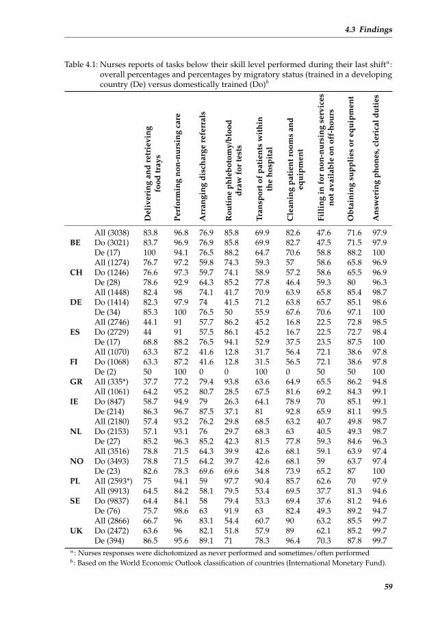
4.3 Findings
Table 4.1: Nurses reports of tasks below their skill level performed during their last shifta:overall percentages and percentages by migratory status (trained in a developingcountry (De) versus domestically trained (Do)b
Del
iver
ing
and
retr
ievi
ngfo
odtr
ays
Perf
orm
ing
non-
nurs
ing
care
Arr
angi
ngdi
scha
rge
refe
rral
s
Rou
tine
phle
boto
my/
bloo
ddr
awfo
rte
sts
Tran
spor
tof
pati
ents
wit
hin
the
hosp
ital
Cle
anin
gpa
tien
troo
ms
and
equi
pmen
t
Fill
ing
info
rno
n-nu
rsin
gse
rvic
esno
tava
ilab
leon
off-
hour
s
Obt
aini
ngsu
ppli
esor
equi
pmen
t
Ans
wer
ing
phon
es,c
leri
cald
utie
s
BEAll (3038) 83.8 96.8 76.9 85.8 69.9 82.6 47.6 71.6 97.9Do (3021) 83.7 96.9 76.9 85.8 69.9 82.7 47.5 71.5 97.9De (17) 100 94.1 76.5 88.2 64.7 70.6 58.8 88.2 100
CHAll (1274) 76.7 97.2 59.8 74.3 59.3 57 58.6 65.8 96.9Do (1246) 76.6 97.3 59.7 74.1 58.9 57.2 58.6 65.5 96.9De (28) 78.6 92.9 64.3 85.2 77.8 46.4 59.3 80 96.3
DEAll (1448) 82.4 98 74.1 41.7 70.9 63.9 65.8 85.4 98.7Do (1414) 82.3 97.9 74 41.5 71.2 63.8 65.7 85.1 98.6De (34) 85.3 100 76.5 50 55.9 67.6 70.6 97.1 100
ESAll (2746) 44.1 91 57.7 86.2 45.2 16.8 22.5 72.8 98.5Do (2729) 44 91 57.5 86.1 45.2 16.7 22.5 72.7 98.4De (17) 68.8 88.2 76.5 94.1 52.9 37.5 23.5 87.5 100
FIAll (1070) 63.3 87.2 41.6 12.8 31.7 56.4 72.1 38.6 97.8Do (1068) 63.3 87.2 41.6 12.8 31.5 56.5 72.1 38.6 97.8De (2) 50 100 0 0 100 0 50 50 100
GR All (335*) 37.7 77.2 79.4 93.8 63.6 64.9 65.5 86.2 94.8
IEAll (1061) 64.2 95.2 80.7 28.5 67.5 81.6 69.2 84.3 99.1Do (847) 58.7 94.9 79 26.3 64.1 78.9 70 85.1 99.1De (214) 86.3 96.7 87.5 37.1 81 92.8 65.9 81.1 99.5
NLAll (2180) 57.4 93.2 76.2 29.8 68.5 63.2 40.7 49.8 98.7Do (2153) 57.1 93.1 76 29.7 68.3 63 40.5 49.3 98.7De (27) 85.2 96.3 85.2 42.3 81.5 77.8 59.3 84.6 96.3
NOAll (3516) 78.8 71.5 64.3 39.9 42.6 68.1 59.1 63.9 97.4Do (3493) 78.8 71.5 64.2 39.7 42.6 68.1 59 63.7 97.4De (23) 82.6 78.3 69.6 69.6 34.8 73.9 65.2 87 100
PL All (2593*) 75 94.1 59 97.7 90.4 85.7 62.6 70 97.9
SEAll (9913) 64.5 84.2 58.1 79.5 53.4 69.5 37.7 81.3 94.6Do (9837) 64.4 84.1 58 79.4 53.3 69.4 37.6 81.2 94.6De (76) 75.7 98.6 63 91.9 63 82.4 49.3 89.2 94.7
UKAll (2866) 66.7 96 83.1 54.4 60.7 90 63.2 85.5 99.7Do (2472) 63.6 96 82.1 51.8 57.9 89 62.1 85.2 99.7De (394) 86.5 95.6 89.1 71 78.3 96.4 70.3 87.8 99.7
a: Nurses responses were dichotomized as never performed and sometimes/often performedb: Based on the World Economic Outlook classification of countries (International Monetary Fund).
59
Chapter 4 A multi-country ... from developing countries
out of 25 trusts, Philippine-trained nurses compared to domestically trained nurses moreoften reported they had delivered and retrieved food trays during their last shift. This wasalso the case in 19 out of 20 Irish hospitals where Philippine-trained nurses were working.
The intraclass correlation coefficient for the nine items varied from .08 to .35, and was.21 for the composite measure, justifying the need for specifying a multilevel model. Table4.2 displays that after adjusting for last shift worked, years of experience, and level of edu-cation, there remained a pronounced overall effect of being a foreign trained nurse from adeveloping country and an increase in reports of tasks performed during the last shift. Thisoverall effect was found for the model testing the association between nurses migratorystatus and the composite measure of tasks performed during the last shift. The interactioneffect for this analysis was non-significant. The series of models to analyze the overall effectof migratory status on each task separately showed that for eight out of nine tasks therewas an overall effect of being a foreign trained nurse from a developing country and anincrease in reporting those tasks. Being a foreign trained nurse from a developing countrywas a significant predictor of all five tasks for which an interaction effect was specified. Theinteraction effect was non-significant for three tasks (arranging discharge referrals, routinephlebotomy/blood draw for tests, cleaning patient rooms and equipment). For deliveringand retrieving food trays and obtaining supplies or equipment, the interaction effect wassignificant. For three out of four tasks for which no interaction effect could be specified, be-ing a foreign trained nurse from a developing country was a significant predictor (perform-ing non-nursing care, transport of patients within the hospital, filling in for non-nursingservices not available on off-hours). Migratory status failed to predict the task of answeringphones, clerical duties, for which in each country at least 90% of both domestically trainednurses and foreign trained nurses reported they had performed this task during their lastshift (Figure 4.2).
4.4 Discussion
This study documented high proportions of nurses across twelve countries indicating theyhad performed tasks below their skill level during their last shift. These findings supportthe previous studies of Aiken et al. (2001), Desjardins et al. (2008); Hendrich et al. (2008) inwhich nurses reported much time spend on non-nursing tasks or much time wasted duringtheir last shift.
Findings also revealed that, while a high share of all nurses reported having performedtasks below their skill level during their last shift, being a foreign trained nurse from adeveloping country was a significant predictor of performing tasks below skill level. Thesefindings resulted from a two-level logistic random effects regression model testing the over-all effect of migratory status on a composite measure of tasks performed, and persisted fora series of two-level random effects regression models to analyze the overall effect of migra-tory status on each task separately. The consistency in results across countries and hospitalsmakes these findings compelling.
In 2010, the World Health Assembly adopted the WHO Global Code of Practice on the
60

4.4 Discussion
Figure 4.2: Nurses reports of tasks below their skill level performed during their lastshift. Heat map comparing reports from domestically trained nurses and nursestrained in a developing country.
61

Chapter 4 A multi-country ... from developing countries
Table 4.2: Logistic random effects modelsa estimating the overall effect of nurses migratorystatus (trained in a developing country versus domestically trainedb across eightcountriesc on task below skill level performed during nurses last shift
Tasks performed during nurses last shift Estimate Odds ratio (95% CI) p-Value
Composite measure of nine nursing tasks 0.74 2.10 (1.68–2.61) <0.0001Delivering and retrieving food traysd 1.65 5.21 (4.04–6.72) <0.0001Performing non-nursing caree 0.53 1.70 (1.13–2.56) 0.014Arranging discharge referralsd 0.89 2.44 (1.92–3.08) <0.0001Routine phlebotomy/blood draw for testsd 0.90 2.46 (1.91–3.17) <0.0001Transport of patients within the hospitale 0.73 2.08 (1.71–2.52) <0.0001Cleaning patient rooms and equipmentd 0.64 1.90 (1.44–2.50) <0.0001Filling in for non-nursing services 0.19 1.21 (0.99–1.47) 0.048not available on off-hourse
Obtaining supplies or equipmentd 0.30 1.35 (1.03–1.78) 0.033Answering phones, clerical dutiese 0.53 1.70 (0.70–4.10) 0.235a: Adjusted for last shift worked (morning, evening, night as reported by the nurses), number of
years worked as a nurse and degree obtained (bachelor degree or not)b: Based on the World Economic Outlook classification of countries (International Monetary Fund)c: England, Germany, Ireland, Netherlands, Norway, Spain, Sweden, Switzerlandd: Interaction effect specifiede: No interaction effect specified due to computational problems
International Recruitment of Health Personnel (World Health Organization, 2010). The am-bition of this first code global in scope is for WHO Member States to refrain from the activerecruitment of health personnel from developing countries facing critical shortages of healthworkers. The code also emphasizes the importance of equal treatment for migrant healthworkers and the domestically trained health workforce.
The RN4CAST data provided an opportunity to contribute to our understanding of thislimited topic of research. The mix of countries participating in this study reflects the diver-sity of health systems in Europe, ensuring a rich perspective of nursing workforce issuesfrom all angles. We used robust statistical techniques to analyze the differences amongdomestically trained nurses and foreign trained nurses from developing countries. Theproportion of foreign trained nurses from developing or from developed countries corre-sponded closely to that observed by the OECD (Organisation for Economic Cooperationand Development, 2010).
Several limitations warrant consideration. First, our measure of migratory status maynot have captured adequately the nationality of the nurse since only the country of train-ing was known. Second, the proportion of foreign trained nurses to the total sample wasrather small. From the twelve countries under study, we had to drop from our analysis threecountries with low numbers of foreign trained nurses from developing countries (Finland,Greece, Poland) and one country with high missing values on the variable of country oftraining. Third, the list of items on tasks below nurses skill level was investigator-developed(Aiken et al., 2001). However, it has shown to have predictive validity to the incompletion
62

4.5 Conclusion
of nursing activities (Al-Kandari and Thomas, 2009). Also, other authors used similar itemsto describe waste (Hendrich et al., 2008) or non-nursing tasks (Desjardins et al., 2008). Anearly work measurement study from Connor (1961) already identified activities such ashousekeeping and dietary tray delivery as non-nursing activities. It are exactly these tasksthat could be delegated to non-nursing personnel (O’Brien-Pallas et al., 2004). It is how-ever conceivable that some tasks surveyed here in certain situations of care were indeednursing tasks. It is also possible that we have not captured all tasks below nurses skill level.Last, in this multi-country European context, consideration is warranted since the context inwhich nurses performed these tasks can be very diverse. The influence of professional prac-tice standards, skill levels of foreign trained nurses from developing countries and valuesattached to these tasks resulting from previous work experiences in their home countrieswas unknown. We did not know for example whether foreign trained nurses from devel-oping countries were more likely than domestic trained nurses to be assigned to performtasks below their skill level or whether foreign trained nurses were more task oriented andbrought the customs and roles of nursing from their developing country backgrounds intodeveloped countries and are thus more prone to voluntarily take on tasks below their skilllevel. The differences we found between reports from domestically trained nurses and for-eign trained nurses were, however, not attributable to lower level of education or less yearsof experience. To the contrary, in each country the foreign trained nurses from developingcountries had significantly more experience in working as a nurse compared to domesti-cally trained nurses. We did not know however how long they had been working as a nursein their destination country. Lastly, future research should assess whether performing moretasks below the skill level is a barrier to providing good patient care or results in lowernurse wellbeing.
4.5 Conclusion
The findings suggest that there remains much room for improvement to optimize the use ofnurses time and energy. Human resources management should give more attention to pro-fessional socialization and life-long learning for nurses to improve their priority setting andtime management as well as ensuing that non-nursing resources are designated to carry outtasks that do not require the unique training of professional nurses. Nurses from developingcountries may be particularly in need of continuing education on professional nurse rolesand responsibilities in complex healthcare settings. Further research is needed to under-stand the influence of professional practice standards, skill levels of foreign trained nursesfrom developing countries and values attached to these tasks resulting from previous workexperiences in their home countries. This will allow us to better understand the conditionsunder which foreign trained nurses from developing countries performed these tasks andto support improved structuring their work.
63
Chapter 4 A multi-country ... from developing countries
References
Aiken, L. H., Clarke, S. P., Sloane, D. M., Sochalski, J. A., Busse, R., Clarke, H., Giovannetti,P., Hunt, J., Rafferty, A. M., and Shamian, J. (2001). Nurses’ reports on hospital care in fivecountries. Health Affairs, 20(3):43–53.
Aiken, L. H., Sermeus, W., Van den Heede, K., Sloane, D. M., Busse, R., McKee, M.,Bruyneel, L., Rafferty, A. M., Griffiths, P., Moreno-Casbas, M. T., et al. (2012). Patient safety,satisfaction, and quality of hospital care: Cross sectional surveys of nurses and patients in12 countries in Europe and the United States. BMJ: British Medical Journal, 344:e1717.
Al-Kandari, F. and Thomas, D. (2009). Factors contributing to nursing task incompletionas perceived by nurses working in kuwait general hospitals. J Clin Nurs, 18(24):3430–3440.
Center for Health Workforce Studies (2008). The hospital nursing workforce in New York:Findings from a survey of hospital registered nurses.
Connor, R. J. (1961). A work sampling study of variations in nursing work load. Hospitals,35:40–41.
Desjardins, F., Cardinal, L., Belzile, E., and McCusker, J. (2008). Reorganizing nursing workon surgical units: a time-and-motion study. Nurs Leadersh (Tor Ont), 21(3):26–38.
Flynn, L. and Aiken, L. H. (2002). Does international nurse recruitment influence practicevalues in us hospitals? Journal of Nursing Scholarship, 34(1):67–73.
Hendrich, A., Chow, M. P., Skierczynski, B. A., and Lu, Z. (2008). A 36-hospital time andmotion study: how do medical-surgical nurses spend their time? The Permanente Journal,12(3):25–34.
Humphries, N., Brugha, R., and McGee, H. (2009). Career progression of migrant nurses inireland: Nurse migration project policy brief 5. Technical report, Royal College of Surgeonsin Ireland, Dublin.
Kelly, L. A., McHugh, M. D., and Aiken, L. H. (2012). Nurse outcomes in magnet andnon-magnet hospitals. J Nurs Adm, 42(10 Suppl):S44–S49.
Kline, D. S. (2003). Push and pull factors in international nurse migration. J Nurs Scholarsh,35(2):107–111.
O’Brien-Pallas, L., Thomson, D., Hall, M., Pink, G., Kerr, M., Wang, S., Li, X., and Meyer,R. (2004). Evidence-based standards for measuring nurse staffing and performance. CanadianHealth Services Research Foundation (Fondation canadienne de la recherche sur les ser-vices de sante).
Organisation for Economic Cooperation and Development (2010). Policy Brief February2010. International Migration of Health Workers. Improving International Co-operation toAddress the Global Health Workforce Crisis.
Sermeus, W., Aiken, L., Van den Heede, K., Rafferty, A., Griffiths, P., Moreno-Casbas, M.,Busse, R., Lindqvist, R., Scott, A., Bruyneel, L., et al. (2011). Nurse forecasting in Europe(RN4CAST): Rationale, design and methodology. BMC Nursing, 10(1):6.
Sneath, P. H. (1957). The application of computers to taxonomy. Journal of general microbi-ology, 17(1):201–226.
World Health Organization (2010). The WHO Global Code of Practice on the InternationalRecruitment of Health Personnel.
64
5NURSING UNIT MANAGERS AND STAFF
NURSES OPINIONS OF THE NURSINGWORK ENVIRONMENT: A BAYESIAN
MULTILEVEL MIMIC MODEL FORCROSS-GROUP COMPARISONS
Chapter 5 is based on the paper:Bruyneel, L., Li, B., Squires, A., Gilmartin, M., Spotbeen, S., Meuleman, B., Lesaffre, E., and Ser-meus, W. (2014). Nursing unit managers’ and staff nurses’ opinions of the nursing work envi-ronment: a Bayesian multilevel mimic model for cross-group comparisons. Research in Nursing &Health (submitted)
65
Chapter 5 Nursing unit managers ... cross-group comparisons
Abstract
The objective of this study is to effectively compare nursing unit man-agers and staff nurses opinions of the nursing work environment (mea-sured by the PES-NWI) by means of a state-of-the- art statistical ap-proach. A Bayesian two-level MIMIC model is performed to evaluatemeasurement invariance as a logical prerequisite to addressing cross-group comparisons. Our findings provide evidence that the PES-NWI isto a great degree invariant in evaluating nursing work environment per-ceptions across nurse managers and staff nurses, and across languagegroups. Further, nursing unit managers evaluated certain importantnurse work environment dimensions more positively when comparedto their staff nurses. This might influence organizational change imple-mentation. Implications for both analytic methods in cross-sectional or-ganizational analyses and cross-cultural research are discussed.
66
5.1 Introduction
5.1 Introduction
Health services researchers frequently use comparative surveys to detect and explain dif-ferences between (sub)groups of respondents. An important research domain where groupcomparisons are a core component is nursing outcomes research. This research studies howthe organization of nursing care (workload, education, work environment) is associatedwith patient safety and nurse wellbeing (Lake, 2007). Studies on the quality of nurses workenvironment have recently received significant attention in the leading medical and healthpolicy journals. The field defines the nursing work environment as not only the resourcesand physical environment where a nurse works, but also includes nurses in governance ac-tivities, quality of workplace relationships, and quality of nurse management. Many valu-able insights about the organizational dynamics behind nursing role implementation in theacute care setting have resulted from research on nurses work environment. Good hospi-tal work environments are associated with higher rates of nurse wellbeing (Aiken et al.,2012; Kelly et al., 2011), superior patient experiences with hospital care (Aiken et al., 2012;Kutney-Lee et al., 2009) and lower patient in-hospital mortality (Aiken et al., 2008; Frieseet al., 2008). Moreover, a positive work environment is a prerequisite for benefiting frombetter nurse staffing (Aiken et al., 2011).
One of the critical factors in the nursing work environment that has been consistentlyidentified in explaining improved nurse wellbeing, is that of quality of nurse management(Gunnarsdttir et al., 2009; Duffield et al., 2011; Kleinman, 2004). This evidence results fromstaff nurses perceptions of their managers. Other hospital organizational research studiesused a different and perhaps more interesting study design by bringing together both front-line workers and managers views on the topic of interest. These studies suggest divergentviews between hospital frontline workers and management on several features in the orga-nization of hospital care. Price et al. (2007) showed that clinical nurses and their managersoffered divergent views of deficiencies in quality improvement implementation. Kalischand Lee (2012) found that nurse leaders reported more missed nursing care and higherteamwork, but less problems with having adequate material and labor resources than didnursing staff members. Studies including several types of hospital staff found that man-agers have a more positive perception of the patient safety climate (Singer et al., 2008) andperceive greater improvements in patient safety culture, but lower improvements on thetimeliness of care delivery (Parand et al., 2011). Similar chasms in staff nurses and nursingunit managers perceptions of the nursing work environment have not been studied previ-ously.
A main issue in comparative research is that the observed differences may be biased asa result of the measurement instrument not functioning invariantly across groups beingcompared (Vandenberg and Lance, 2000). Measurement invariance pertains to the extentto which respondents across groups perceive and interpret the content of items in the sameway (Byrne and Watkins, 2003). Lack of measurement invariance is also referred to as dif-ferential item functioning (DIF). This could lead to serious erroneous inference and thusincorrect research findings and implications. Health services researchers increasingly advo-
67
Chapter 5 Nursing unit managers ... cross-group comparisons
cate for the incorporation of measurement invariance detection techniques in the analyticstrategy (Cherepanov et al., 2011; Borsboom, 2006), yet such evaluations have been notablyabsent from the literature. Recent advancements in computational statistics for measure-ment invariance evaluation have greatly enhanced the feasibility of studies focusing on thisimportant part of psychometric evaluation of measurement tools.
The aim of this study is to effectively evaluate cross-group differences in nursing unitmanagers and staff nurses opinions of the nursing work environment by means of a state-of-the-art statistical approach. Nurse managers have an immensely important role in takingimmediate action to remedy work environment issues reported by staff nurses. For optimalpatient outcomes, nurse managers and their staff nurses must, therefore, have concordantviews about the quality of the nursing work environment. In line with the aforementionedresearch findings, in which managers generally tend to have more positive views on featuresof hospital care, we posit that nurse managers compared to staff nurses have more positiveviews of nurses work environment. When comparing groups, the assumption of measure-ment invariance must be tested in order to adequately capture the scope of these differences.No prior empirical work has tested the measurement invariance assumption among nursemanagers and staff nurses ratings of the nursing work environment. We therefore had no apriori hypotheses regarding work environment items exhibiting DIF.
5.2 Method
Study setting
This study analyzes a convenience sample of one large Belgian hospital entity. Hospitalmanagement identified an opportunity for a hospital-wide assessment of nurses practiceenvironment, staffing, productivity, and their wellbeing, using previously extensively vali-dated instruments from the Registered Nurse Forecasting (RN4CAST) study, a large Euro-pean nurse workforce study funded by the Seventh Framework Programme of the EuropeanUnion (Sermeus et al., 2011). Dutch and French versions of the questionnaire, with transla-tions previously validated (Squires et al., 2013), were distributed to nursing unit managersand staff nurses on 118 patient care nursing units, with exactly one nurse manager per unit.Eighty-seven out of 118 nurse managers completed the questionnaire (75.0% response rate).On these 87 nursing units, 821 out of 1159 staff nurses completed the questionnaire (70.8%response rate). The final data set thus consists of 908 observations. For the purpose of thisstudy, a nursing unit manager is defined as a registered nurse who is largely responsible foradministratively and clinically managing the nursing staff on a given nursing unit.
Study design
Nursing unit managers and staff nurses perceptions of the nursing work environment weremeasured using the practice environment scale of the nursing work index (PES-NWI) (Lake,2002). This instrument was derived from a long line of successful research on nurses work-ing conditions that began with research by Kramer and Hafner (1989) on magnet hospitals.Their initial instrument measured elements of nurse job satisfaction and nurse perceptions
68
5.2 Method
of the quality of care. Aiken and Patrician (2000) further refined the instrument into theRevised Nursing Work Index (NWI-R), to determine the aspects of the professional workenvironment. The PES-NWI consists of 32 statements measured on a 4-point Likert scaleanchored between 1=completely disagree to 4=completely agree. In the factor analytic stageof the development of the PES-NWI, Lake (2002) proposed five dimensions of the nurs-ing work environment. These include collegial nurse-physician relations; nurse managerialabilities, leadership, and support of nurses; nurse participation in hospital affairs; nurs-ing foundations for quality of care; and staffing and resource adequacy. The United StatesNational Quality Forum endorses this instrument for use in nursing-sensitive care perfor-mance measurement and globally, it has shown good internal consistency and validity (War-shawsky and Havens, 2011).
Statistical methods
A two-level structural equation model is applied as the analytic strategy. The methods areexplained within a methodological framework that is largely based on recent innovativestatistical advancements by Muthen and Asparouhov (2012). These techniques may applyequally well to many other studies in the field of health services research and beyond.
We propose the following arguments for supporting our analytic approach. First, ourinstrument that measures the work environment, the PES-NWI, consists of various latentvariables (nursing work environment dimensions) which should be accounted for in thestatistical analysis. Although exploratory factor analytic techniques are often used to assessthe psychometric properties of the PES-NWI (Warshawsky and Havens, 2011), the commonpractice is to calculate subscale scores by taking the average of the item scores. These newlycreated variables are subsequently used in regression analysis. Structural equation model-ing provides an alternative approach. This model is able to test complete and simultaneousrelationships between complex and multidimensional phenomena (Tabachnick and Fidell,2012).
Second, the research design of most comparative, cross-sectional studies involves clus-tered data. Nurse workforce studies, for example, involve nurses clustered in various or-ganizational levels, such as nursing units within hospitals. Ignoring a multilevel structurein the analysis can be problematic since the fundamental independence assumption under-lying many commonly used statistical techniques is violated (Muthen, 1991). Gabriel et al.(2013); Li et al. (2013) recently conducted multilevel PES-NWI analyses, with two and fourlevels respectively, showing how different PES-NWI dimensions predict nurse wellbeing atdifferent levels. The PES-NWI has also previously been analyzed in a two-level confirma-tory factor analytic framework by Gajewski et al. (2010) and Gabriel et al. (2013).
To compensate for the aforementioned analytic issues, we handled the clustered and la-tent nature of our measures by estimating two-level factor models with nurses clustered innursing units. In these models we accounted for the categorical nature of the data. First,to assess the multidimensionality of the PES-NWI, we adopted a two-level exploratory fac-tor analytic model (EFA) with Geomin rotation. EFA is extremely useful to understand thefactor structure and evaluate whether items are misbehaving. An exploratory analysis was
69
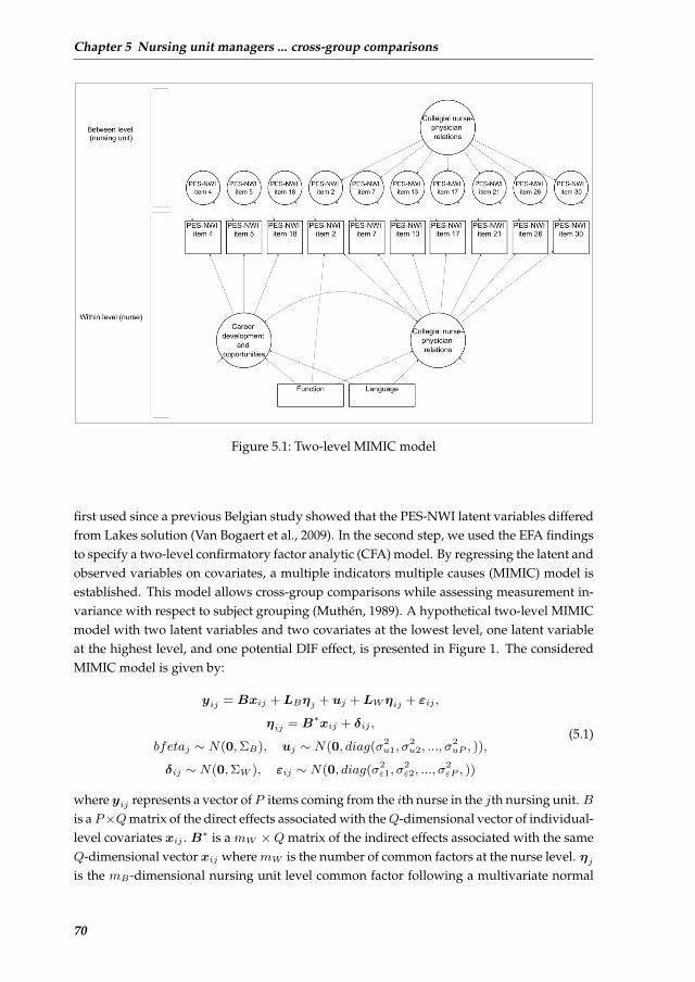
Chapter 5 Nursing unit managers ... cross-group comparisons
21
FIGURES
Figure 1. Two-level MIMIC model
Figure 5.1: Two-level MIMIC model
first used since a previous Belgian study showed that the PES-NWI latent variables differedfrom Lakes solution (Van Bogaert et al., 2009). In the second step, we used the EFA findingsto specify a two-level confirmatory factor analytic (CFA) model. By regressing the latent andobserved variables on covariates, a multiple indicators multiple causes (MIMIC) model isestablished. This model allows cross-group comparisons while assessing measurement in-variance with respect to subject grouping (Muthen, 1989). A hypothetical two-level MIMICmodel with two latent variables and two covariates at the lowest level, one latent variableat the highest level, and one potential DIF effect, is presented in Figure 1. The consideredMIMIC model is given by:
yij = Bxij + LBηj + uj + LWηij + εij ,
ηij = B∗xij + δij ,
bfetaj ∼ N(0,ΣB), uj ∼ N(0, diag(σ2u1, σ
2u2, ..., σ
2uP , )),
δij ∼ N(0,ΣW ), εij ∼ N(0, diag(σ2ε1, σ
2ε2, ..., σ
2εP , ))
(5.1)
where yij represents a vector ofP items coming from the ith nurse in the jth nursing unit. Bis a P×Qmatrix of the direct effects associated with theQ-dimensional vector of individual-level covariates xij . B∗ is a mW ×Q matrix of the indirect effects associated with the sameQ-dimensional vector xij wheremW is the number of common factors at the nurse level. ηjis the mB-dimensional nursing unit level common factor following a multivariate normal
70
5.2 Method
distribution with mean zero and a covariate matrix ΣB , andLB is its P×mB loading matrixwithmB the number of common factors at the nursing unit level. ηij is themW -dimensionalnurse level common factors with a multivariate normal distribution with mean zero and acovariance matrix ΣW , and LW is its loading matrix with a P ×mW dimension. uj is theP-dimensional random intercept with independent normal distribution for each elementwith mean zero and a variance σ2
up, while εij is the P -dimensional residual, each elementof which follows an independent normal distribution with mean zero and a variance σ2
εp.From the MIMIC model, one can capture cross-group differences if there is a significant
effect of a covariate on a latent variable, indicating that the factor means are different fordifferent levels of the covariates. For this study, for example, an effect of the main covariateof interest, nurses function (nursing unit manager versus staff nurse) on any of the PES-NWI latent variables would indicate that the latent variable mean is different for nursingunit managers and staff nurses. DIF can be examined by estimating direct effects betweena covariate and the observed variables. A covariate having a direct effect on an observedvariable (over and above the indirect effect via the factors), indicates that the average re-sponse differs across respondents with different values for the covariate but the same scoreon the latent factor. In other words, direct effects represent violations of the assumption ofmeasurement invariance 1 (Muthen, 1989). For this study, for example, a direct effect be-tween the covariate on nurses function and one of the 32 PES-NWI items, over and abovethe indirect effect via the factors, would indicate that this particular item does not behavethe same for nursing unit managers and staff nurses.
Previous research using the PES-NWI has not always adequately accounted for confound-ing variables. Jak et al. (2010) advise researchers investigating measurement bias to in-clude as many possible violator variables as available. Possible confounders and respec-tive coding included in the analysis are nurses language (0 =French, 1 =Dutch), degree(0 =diploma degree, 1 =bachelor degree), type of employment (0 =part-time, 1 =full-time), migratory status (0 =domestically trained, 1 =foreign trained) and gender (0 =female,1 =male).
We adopted a Bayesian structural equation modeling (BSEM) approach to identify themodel Muthen and Asparouhov (2012). This Bayesian approach was recently applied byFong and Ho (2013) to evaluate the latent structure of a measurement instrument to as-sess and screen symptoms of anxiety and depression. In contrast to a frequentist approach,substantive information can be included in the model. Here, it is useful to include such in-formation in the form of small-variance priors. Informative priors for the cross-loadings canrestrict them stochastically, thereby overcoming possible identification problems. The finalmodel is a Bayesian two-level MIMIC model with cross-loadings and direct effects from thecovariates to the items with zero mean and small-variance priors, 0.05 and 0.1 respectively,based on prior factor analytic findings and drawing on Muthen and Asparouhov (2012)
1Such differences in conditional item means i.e. scalar non-invariance (Steenkamp and Baumgartner, 1998) repre-sent only one possible form of measurement non-invariance, besides for example metric non-invariance (inequal-ity of the strength of the relationships between indicators and latent factors Steenkamp and Baumgartner (1998)).Testing metric invariance within our MIMIC approach is less straightforward, and would imply including an im-practically large number of interaction effects. Yet, scalar invariance implies stronger assumptions and thus a morestringent test than metric invariance, which justifies our approach (see also Muthen (1989))
71

Chapter 5 Nursing unit managers ... cross-group comparisons
simulation modeling approach. Muthen and Asparouhov (2013) described the importanceof prior variance choosing in detecting non-invariance. A larger value for a prior variancemay result in an increase in both the standard error of the parameter and the chances thatthe estimate can escape from the invariance value. Models with different values for the priorvariance were therefore performed. Findings across models turned out to be very stable.
For both EFA and CFA entries the standardized model results are presented. The boldedentries presented in EFA and CFA findings are loadings that are largest for the item. Anadditional requirement for the entry to be bolded is that the loading must exceed a value of.3 and no severe cross-loadings can be present. Significant effects, meaning that the Bayesiancredibility interval did not cover zero, are marked with an asterisk. Intra class correlations(ICC) are presented, which reflect the proportion of a single variables variance that can beaccounted for by the ”between” level. In addition we looked at the design effect, which isa function of the average cluster size and ICC, and is calculated as ϕ = 1 + (n − 1) ∗ ICC,where n equals the average group size. A design effect larger than two indicates that theclustering in the data needs to be taken into account during estimation Satorra and Muthen(1995). Evaluation of good EFA model fit between the hypothesized model and the observeddata is based on Hu and Bentler (1999) suggestions to have cutoff values close to or above0.95 for Tucker Lewis Index (TLI) and Comparative Fit Index (CFI), below or close to 0.08for the standardized root mean square residual (SRMR), and below or close to 0.06 for theroot mean square error of approximation (RMSEA). SAS Version 9.3 of the SAS System forWindows was used for descriptive analysis and to prepare data for further analyses. MplusVersion 7 was used for structural equation modeling (Muthen and Muthen, 2010).
5.3 Results
We begin this section with a description of the final sample size and follow with resultsspecific to each type of analysis we conducted. The results begin with findings from thetwo-level exploratory factor analysis. Then, we describe the results from the MIMIC model.
Sample characteristics
The response rate at the unit level varied from 23.1% to 100%. Seventy-eight out of 87nursing units had a response rate above 50%. The number of nurses per nursing unit variedfrom 3 to 27 (mean= 9.4, median= 9).
Table 5.1 displays the personal characteristics for nursing unit managers and staff nursesseparately. The majority of nurses were female, spoke French, had obtained a bachelor de-gree, were domestically educated and worked full-time. A considerably higher proportionof nursing unit managers compared to staff nurses worked full-time and were domesticallyeducated.
Two-level exploratory factor analysis
Table 5.2 displays the findings of the two-level exploratory factor analysis. Also includedin this table are the factor structure of Lake (2002) as well as the ICC values. Twenty-one
72
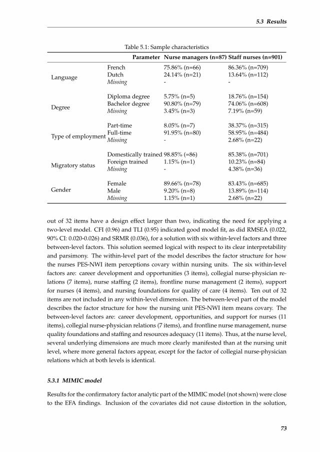
5.3 Results
Table 5.1: Sample characteristics
Parameter Nurse managers (n=87) Staff nurses (n=901)
Language
French 75.86% (n=66) 86.36% (n=709)Dutch 24.14% (n=21) 13.64% (n=112)Missing - -
Degree
Diploma degree 5.75% (n=5) 18.76% (n=154)Bachelor degree 90.80% (n=79) 74.06% (n=608)Missing 3.45% (n=3) 7.19% (n=59)
Type of employment
Part-time 8.05% (n=7) 38.37% (n=315)Full-time 91.95% (n=80) 58.95% (n=484)Missing - 2.68% (n=22)
Migratory status
Domestically trained 98.85% (=86) 85.38% (n=701)Foreign trained 1.15% (n=1) 10.23% (n=84)Missing - 4.38% (n=36)
GenderFemale 89.66% (n=78) 83.43% (n=685)Male 9.20% (n=8) 13.89% (n=114)Missing 1.15% (n=1) 2.68% (n=22)
out of 32 items have a design effect larger than two, indicating the need for applying atwo-level model. CFI (0.96) and TLI (0.95) indicated good model fit, as did RMSEA (0.022,90% CI: 0.020-0.026) and SRMR (0.036), for a solution with six within-level factors and threebetween-level factors. This solution seemed logical with respect to its clear interpretabilityand parsimony. The within-level part of the model describes the factor structure for howthe nurses PES-NWI item perceptions covary within nursing units. The six within-levelfactors are: career development and opportunities (3 items), collegial nurse-physician re-lations (7 items), nurse staffing (2 items), frontline nurse management (2 items), supportfor nurses (4 items), and nursing foundations for quality of care (4 items). Ten out of 32items are not included in any within-level dimension. The between-level part of the modeldescribes the factor structure for how the nursing unit PES-NWI item means covary. Thebetween-level factors are: career development, opportunities, and support for nurses (11items), collegial nurse-physician relations (7 items), and frontline nurse management, nursequality foundations and staffing and resources adequacy (11 items). Thus, at the nurse level,several underlying dimensions are much more clearly manifested than at the nursing unitlevel, where more general factors appear, except for the factor of collegial nurse-physicianrelations which at both levels is identical.
5.3.1 MIMIC model
Results for the confirmatory factor analytic part of the MIMIC model (not shown) were closeto the EFA findings. Inclusion of the covariates did not cause distortion in the solution,
73
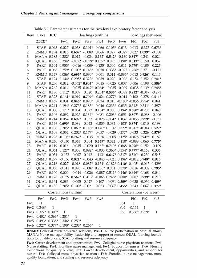
Chapter 5 Nursing unit managers ... cross-group comparisons
Table 5.2: Parameter estimates for the two-level exploratory factor analysis
Item Lake ICC loadings (within) loadings (between)
(2002)* Fw1 Fw2 Fw3 Fw4 Fw5 Fw6 Fb1 Fb2 Fb3
1 STAF 0.045 0.027 0.058 0.191* 0.066 0.105* 0.013 0.013 -0.375 0.673*2 RNMD 0.194 0.016 0.687* -0.089 0.066 0.027 -0.029 0.027 1.039* -0.0883 MANA 0.183 0.282* 0.012 -0.034 0.152* 0.542* -0.130 0.847* 0.241 0.0244 QUAL 0.168 0.394* -0.052 -0.079* 0.169* 0.095 0.190* 0.813* 0.150 0.0575 PART 0.104 0.953* -0.016 -0.009 -0.135* 0.000 0.011 0.779* 0.105 0.2256 PART 0.068 0.259* 0.109* 0.148* 0.038 0.335* -0.027 1.206* 0.371 -0.1217 RNMD 0.147 0.086* 0.695* 0.080* 0.001 0.014 -0.086* 0.013 0.926* 0.1458 STAF 0.124 0.144* 0.295* 0.323* 0.039 0.020 -0.006 -0.154 0.352 0.741*9 STAF 0.230 0.012 -0.062* 0.903* 0.015 -0.025 0.037 0.006 0.198 0.586*10 MANA 0.262 0.014 -0.025 0.047* 0.934* -0.035 -0.009 -0.038 0.139 0.745*11 PART 0.180 0.112* 0.059 0.020 0.204* 0.505* -0.088 0.932* -0.047 -0.27112 STAF 0.325 -0.161* 0.019 0.709* -0.024 0.277* -0.014 0.102 0.278 0.511*13 RNMD 0.167 0.031 0.845* 0.070* 0.034 0.015 -0.180* -0.056 0.974* 0.04114 MANA 0.241 0.194* 0.273* 0.183* 0.046 0.233* 0.035 0.343* 0.541* 0.397*15 QUAL 0.080 0.171* 0.034 0.022 0.164* 0.050 0.194* 0.680* -0.205 0.04816 PART 0.106 0.092 0.025 0.134* 0.081 0.203* 0.051 0.807* -0.068 -0.00617 RNMD 0.214 0.064 0.692* 0.032 -0.026 -0.042 0.037 -0.056 0.979* -0.03118 PART 0.146 0.690* 0.039 0.042 -0.005 0.032 0.103* 0.874* 0.010 0.19819 QUAL 0.108 0.205* 0.069* 0.118* 0.140* 0.114* 0.322* 0.313* -0.014 0.527*20 QUAL 0.109 0.052 0.202* 0.177* 0.057 -0.029 0.277* 0.033 0.326 0.579*21 RNMD 0.223 -0.108* 0.762* -0.035 0.026 -0.005 0.125* -0.028 0.947* 0.18222 MANA 0.260 -0.030 0.063 0.004 0.659* 0.022 0.110* -0.088 0.065 0.775*23 PART 0.119 0.016 -0.035 -0.020 0.162* 0.740* 0.068 0.996* 0.152 -0.10924 QUAL 0.061 0.127* 0.038 0.092* -0.033 0.363* 0.354* 0.777* -0.168 0.33625 PART 0.034 -0.022 -0.007 0.042 -.113* 0.647* 0.317* 0.540* -0.230 0.54526 RNMD 0.277 -0.036 0.821* -0.043 -0.045 -0.021 0.196* -0.012 0.948* 0.01627 QUAL 0.216 0.027 0.018 0.087* 0.134* 0.182* 0.410* 0.405* -0.047 0.429*28 QUAL 0.058 -0.041 0.096 -0.087 0.206* 0.081 0.379* 0.016 -0.002 0.795*29 PART 0.100 0.000 -0.044 -0.026 -0.087 0.511* 0.446* 0.699* 0.168 0.04430 RNMD 0.178 -0.059 0.562* 0.-017 -0.065 0.248* 0.080* 0.007 0.939* 0.21031 QUAL 0.161 0.083 -0.005 0.027 0.107 -0.091 0.509* 0.038 -0.030 0.409*32 QUAL 0.182 0.205* 0.100* -0.021 0.023 -0.067 0.455* 0.243 0.067 0.372*
Correlations (within) Correlations (between)
Fw1 Fw2 Fw3 Fw4 Fw5 Fw6 Fb1 Fb2 Fb3Fw1 1 Fb1 1Fw2 0.348* 1 Fb2 -0.111 1Fw3 0.327* 0.309* 1 Fb3 0.388* 0.229* 1Fw4 0.402* 0.363* 0.281* 1Fw5 0.493* 0.338* 0.346* 0.259* 1Fw6 0.327* 0.377* 0.190* 0.203* 0.266* 1RNMD: Collegial nurse-physician relations; PART: Nurse participation in hospital affairs;MANA: Nurse manager ability, leadership and support of nurses; QUAL: Nursing founda-tions for quality of care; STAF: Staffing and resource adequacyFw1: Career development and opportunities; Fw2: Collegial nurse-physician relations; Fw3:Nurse staffing; Fw4: Frontline nurse management; Fw5: Support for nurses; Fw6: Nursingfoundations for quality of care; Fb1: Career development, opportunities, and support fornurses; Fb2: Collegial nurse-physician relations; Fb3: Frontline nurse management, nursequality foundations, and staffing and resource adequacy
74
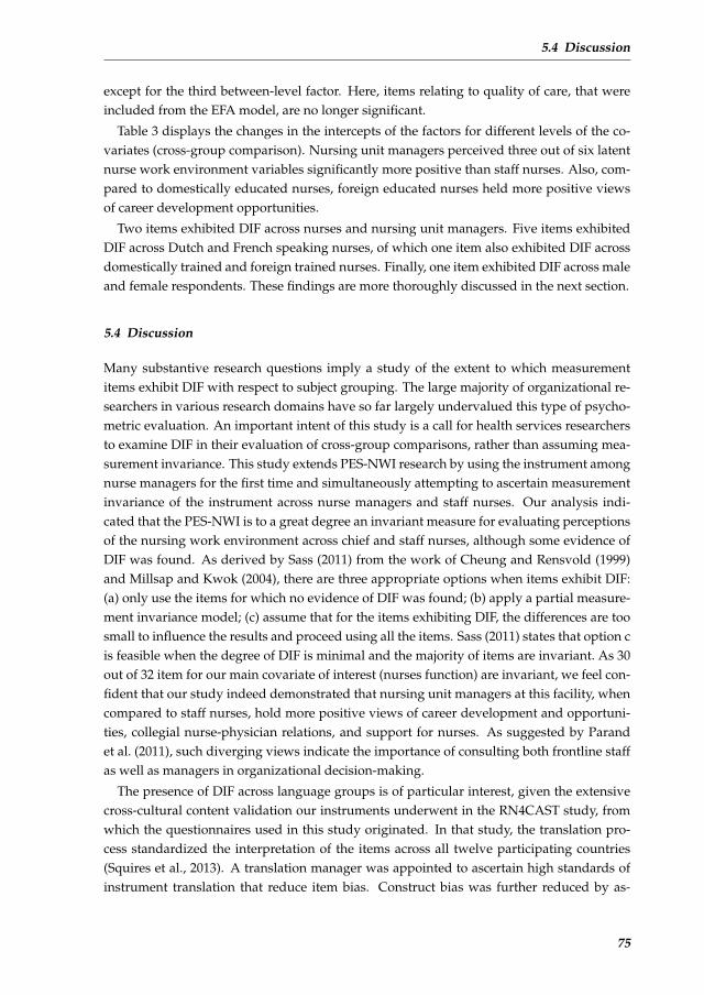
5.4 Discussion
except for the third between-level factor. Here, items relating to quality of care, that wereincluded from the EFA model, are no longer significant.
Table 3 displays the changes in the intercepts of the factors for different levels of the co-variates (cross-group comparison). Nursing unit managers perceived three out of six latentnurse work environment variables significantly more positive than staff nurses. Also, com-pared to domestically educated nurses, foreign educated nurses held more positive viewsof career development opportunities.
Two items exhibited DIF across nurses and nursing unit managers. Five items exhibitedDIF across Dutch and French speaking nurses, of which one item also exhibited DIF acrossdomestically trained and foreign trained nurses. Finally, one item exhibited DIF across maleand female respondents. These findings are more thoroughly discussed in the next section.
5.4 Discussion
Many substantive research questions imply a study of the extent to which measurementitems exhibit DIF with respect to subject grouping. The large majority of organizational re-searchers in various research domains have so far largely undervalued this type of psycho-metric evaluation. An important intent of this study is a call for health services researchersto examine DIF in their evaluation of cross-group comparisons, rather than assuming mea-surement invariance. This study extends PES-NWI research by using the instrument amongnurse managers for the first time and simultaneously attempting to ascertain measurementinvariance of the instrument across nurse managers and staff nurses. Our analysis indi-cated that the PES-NWI is to a great degree an invariant measure for evaluating perceptionsof the nursing work environment across chief and staff nurses, although some evidence ofDIF was found. As derived by Sass (2011) from the work of Cheung and Rensvold (1999)and Millsap and Kwok (2004), there are three appropriate options when items exhibit DIF:(a) only use the items for which no evidence of DIF was found; (b) apply a partial measure-ment invariance model; (c) assume that for the items exhibiting DIF, the differences are toosmall to influence the results and proceed using all the items. Sass (2011) states that option cis feasible when the degree of DIF is minimal and the majority of items are invariant. As 30out of 32 item for our main covariate of interest (nurses function) are invariant, we feel con-fident that our study indeed demonstrated that nursing unit managers at this facility, whencompared to staff nurses, hold more positive views of career development and opportuni-ties, collegial nurse-physician relations, and support for nurses. As suggested by Parandet al. (2011), such diverging views indicate the importance of consulting both frontline staffas well as managers in organizational decision-making.
The presence of DIF across language groups is of particular interest, given the extensivecross-cultural content validation our instruments underwent in the RN4CAST study, fromwhich the questionnaires used in this study originated. In that study, the translation pro-cess standardized the interpretation of the items across all twelve participating countries(Squires et al., 2013). A translation manager was appointed to ascertain high standards ofinstrument translation that reduce item bias. Construct bias was further reduced by as-
75
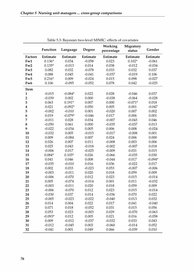
Chapter 5 Nursing unit managers ... cross-group comparisons
Table 5.3: Bayesian two-level MIMIC: effects of covariates
Function Language DegreeWorking Migratory
Genderpercentage status
Factors Estimate Estimate Estimate Estimate Estimate EstimateFw1 0.136* 0.034 -0.058 0.023 0.102* -0.061Fw2 0.135* -0.013 0.014 0.038 -0.012 -0.034Fw3 0.082 0.032 -0.078 0.033 0.032 0.037Fw4 0.088 0.045 -0.041 -0.037 -0.019 0.106Fw5 0.216* 0.009 -0.024 0.015 0.098 -0.027Fw6 0.106 -0.095 -0.052 0.078 0.042 -0.025
Item1 -0.015 -0.084* 0.022 0.028 -0.046 0.0372 -0.039 0.002 0.000 -0.038 -0.064 -0.0283 0.063 0.191* 0.007 0.000 -0.071* 0.0184 0.021 -0.092* 0.050 0.005 0.001 -0.0475 -0.002 -0.010 0.001 -0.020 0.007 0.0026 0.019 -0.079* -0.046 0.017 0.006 0.0017 -0.011 0.028 0.034 -0.007 -0.043 0.0468 -0.050 0.061 0.000 -0.035 -0.037 0.0139 -0.022 -0.034 0.005 0.006 0.008 -0.02410 -0.032 0.005 -0.015 -0.017 -0.008 0.00111 0.009 -0.084 0.007 0.024 0.006 0.00012 0.026 0.007 0.011 -0.008 0.003 0.00613 0.025 0.043 -0.018 -0.002 -0.007 0.01814 -0.006 0.017 -0.025 -0.009 0.031 0.01515 0.084* 0.105* 0.026 -0.066 -0.035 0.03016 0.041 0.046 0.008 -0.044 0.017 -0.094*17 -0.035 -0.010 0.016 0.036 -0.022 0.01718 0.002 0.033 -0.023 0.053 -0.007 -0.00619 -0.003 -0.011 0.020 0.018 0.059 0.00920 -0.006 -0.070 0.012 0.023 0.015 -0.01421 0.005 -0.074 -0.014 0.001 0.011 -0.03222 -0.003 -0.011 0.020 0.018 0.059 0.00923 -0.006 -0.070 0.012 0.023 0.015 -0.01424 -0.030 0.037 0.014 -0.036 0.070 0.02225 -0.005 -0.023 -0.022 -0.040 0.013 0.03226 0.014 0.004 0.022 0.017 0.041 -0.04027 0.071 0.018 -0.052 0.031 0.015 0.05628 0.053 0.023 -0.003 0.029 -0.070 -0.06329 -0.093* 0.012 0.005 0.021 0.016 -0.05830 0.009 -0.012 -0.037 -0.032 0.033 0.04331 -0.012 -0.045 0.003 -0.060 -0.014 0.05232 -0.041 0.001 0.049 0.066 -0.039 0.010
76
5.4 Discussion
sessing dissimilarity of constructs in the investigated countries through the application ofcontent validity indexing procedures. Method bias was decreased by a common samplingand survey administration protocol. It is, therefore, important to further examine whichfactors underlie these findings of DIF.
Limitations
There are a number of methodological challenges that could affect the interpretation of ourfindings. First, with regards to the interpretation of the exploratory factor analytic model,we used Hu and Bentler (1999) recommendations for cut-off values, however, there is stilldisagreement in setting acceptable levels of fit in goodness-of-fit indexes (Marsh et al., 2004).Another drawback related to model fit evaluation in this study, is that the posterior predic-tive p-value that is used in Bayesian analysis, is not yet implemented in Mplus for multilevelanalyses.
Second, although our factor analytic models provided clearly interpretable factors, twoof our factors consisted of two indicators only. To encompass the scope of the construct,Tabachnick and Fidell (2012) recommend at least three indicators per factor since the in-terpretation of the factor defined by less than three variables might be hazardous. It hashowever also been stated that two items per factor can be sufficient, and that this is widelyapplied (Kenny and McCoach, 2003). Important is that the number of included items en-compass the scope of the construct (Bandalos and Finney, 2010). Although specifying onlytwo variables per factor does not necessarily affect model identification, it might be prefer-able to have a larger number of variables per factor to better encompass the scope of thework environment construct. For the factor nurse staffing, only the two items that clearlyreferred to having enough nurses had high factor loadings. In Lakes development of thePES-NWI factor loadings for these two items were also much higher than factor loadingsfor the other two items. The same is true for the two items with highest salience on thefactor of frontline nurse management. Although the conceptual interpretation for these fac-tors can be viewed as perfect subfactors of Lakes original factors, both might benefit fromadding additional items.
Third, we studied measurement invariance in the form of a MIMIC model. An alternativeapproach to study measurement invariance is a multiple group confirmatory factor analytic(MGCFA) model. MGCFA entails the simultaneous analysis of two or more measurementmodels while a MIMIC model involves a single measurement model and input matrix . Ad-vantages of the MGCFA model over the MIMIC model are therefore that it is more flexiblein that it allows more parameters to represent non-invariance. However, the MIMIC modelis more parsimonious and is better suited for analyses where the researcher considers manycovariates jointly, which was the case in this study. Another advantage of MIMIC models isthat it usually has smaller sample size requirements than MGCFA.
77
Chapter 5 Nursing unit managers ... cross-group comparisons
Recommendations for research practice
Two important recommendations emerge from this study for both analytic methods incross-sectional organizational analyses and cross-cultural research.
First, our findings showed interesting instances of between language group variations inthe measurement properties of the PES-NWI. This evidence of measurement non-invariance,even after the many precautions taken in the early stages of the RN4CAST study, suggeststhat researchers need to take precautions for the potential threat of DIF in all stages of theirstudy. An additional tool for examining measurement invariance worth considering in stud-ies that could be affected by cultural dynamics is the technique of anchoring vignettes (Kinget al., 2004). These are descriptions of hypothetical people or situations, included in the datacollection. Anchoring vignettes provide a common scale of measurement, of which the in-formation is used to account for response category differences. As such, they improve theproblems of interpersonal and cross-cultural incomparability in survey research. Anchoringvignettes are highly recommended for research and positive experiences with this techniquehave been reported by various authors (Johnson, 2006; Salomon et al., 2004; Van Soest et al.,2011).
Second, in this study we aligned a multilevel analysis strategy to the level of theory (Kleinet al., 1994). Although we took into account the effects of clustered observations, this can befurther modeled in innovative ways related to the concept of measurement invariance. Jaket al. (2013) recently proposed a method for investigating measurement invariance acrossclusters, illustrating how cluster bias is caused by between-level variables. Also, considerthe recent article of Davidov et al. (2012). Using data from the second round of the EuropeanSocial Survey, the authors demonstrated how measurement non-invariance evidenced byMGCFA can be explained by using multilevel SEM. More specifically, country-level covari-ates allowed the authors to explain why one of their indicators was non-invariant acrosscountries. Including between-level variables should be of particular interest to PES-NWIresearch, since nurse work environment policy decisions are often informed by PES-NWIscore comparisons between hospitals (McHugh et al., 2013) or countries (Aiken et al., 2012).There have been, and will be, numerous studies where these important concepts should becentral to the examination of measurement invariance.
5.5 Conclusion
This study showed that nursing unit managers evaluate certain important nurse work envi-ronment dimensions more positively when compared to their staff nurses. Such chasms be-tween frontline workers and management could destabilize work places, contribute to neg-ative work environments, and could ultimately hinder any possible solutions and strategicdirection to issues raised by frontline nurses to management. Our findings therefore sup-port endeavors to better understand the connection between nursing unit managers andstaff nurses perceptions of their work environment and other organizational features of hos-pital care. Methodologically, evidence of differential item functioning was found throughseveral items that behaved differently for different language groups included in this study.
78
References
This underscores the importance of a rigorous translation procedure and cultural adaptationof items for research studies using instruments developed for measurement in a differenthealthcare system. We hope our application of a method to assess measurement invarianceto health outcomes research linked to healthcare workers, will encourage organizational re-searchers to take on the challenge of applying advanced statistical techniques to verify thesuitability of their analysis to the studys design and implementation challenges.
References
Aiken, L. H., Cimiotti, J. P., Sloane, D. M., Smith, H. L., Flynn, L., and Neff, D. F. (2011). Theeffects of nurse staffing and nurse education on patient deaths in hospitals with differentnurse work environments. Medical Care, 49(12):1047–1053.
Aiken, L. H., Clarke, S. P., Sloane, D. M., Lake, E. T., and Cheney, T. (2008). Effects ofhospital care environment on patient mortality and nurse outcomes. The Journal of NursingAdministration, 38(5):223–229.
Aiken, L. H. and Patrician, P. A. (2000). Measuring organizational traits of hospitals: Therevised nursing work index. Nursing Research, 49(3):146–153.
Aiken, L. H., Sermeus, W., Van den Heede, K., Sloane, D. M., Busse, R., McKee, M.,Bruyneel, L., Rafferty, A. M., Griffiths, P., Moreno-Casbas, M. T., et al. (2012). Patient safety,satisfaction, and quality of hospital care: Cross sectional surveys of nurses and patients in12 countries in Europe and the United States. BMJ: British Medical Journal, 344:e1717.
Bandalos, D. L. and Finney, S. J. (2010). The reviewers guide to quantitative methods in the socialsciences, chapter Factor analysis: Exploratory and confirmatory, pages 93–114. Routledge.
Borsboom, D. (2006). When does measurement invariance matter? Medical Care, 44(11Suppl 3):S176–181.
Byrne, B. M. and Watkins, D. (2003). The issue of measurement invariance revisited. Journalof Cross-Cultural Psychology, 34(2):155–175.
Cherepanov, D., Palta, M., Fryback, D. G., Robert, S. A., Hays, R. D., and Kaplan, R. M.(2011). Gender differences in multiple underlying dimensions of health-related qualityof life are associated with sociodemographic and socioeconomic status. Medical Care,49(11):1021–1030.
Cheung, G. W. and Rensvold, R. B. (1999). Testing factorial invariance across groups: Areconceptualization and proposed new method. Journal of Management, 25(1):1–27.
Davidov, E., Dulmer, H., Schluter, E., Schmidt, P., and Meuleman, B. (2012). Using a mul-tilevel structural equation modeling approach to explain cross-cultural measurement non-invariance. Journal of Cross-Cultural Psychology, 43(4):558–575.
Duffield, C. M., Roche, M. A., Blay, N., and Stasa, H. (2011). Nursing unit managers, staffretention and the work environment. J Clin Nurs, 20(1-2):23–33.
Fong, T. C. T. and Ho, R. T. H. (2013). Factor analyses of the hospital anxiety and de-pression scale: a bayesian structural equation modeling approach. Quality of Life Research,22(10):2857–2863.
Friese, C. R., Lake, E. T., Aiken, L. H., Silber, J. H., and Sochalski, J. (2008). Hospitalnurse practice environments and outcomes for surgical oncology patients. Health ServicesResearch, 43(4):1145–1163.
Gabriel, A. S., Erickson, R. J., Moran, C. M., Diefendorff, J. M., and Bromley, G. E. (2013).A multilevel analysis of the effects of the practice environment scale of the nursing workindex on nurse outcomes. Research in Nursing & Health, 36(6):567–581.
79
Chapter 5 Nursing unit managers ... cross-group comparisons
Gajewski, B. J., Boyle, D. K., Miller, P. A., Oberhelman, F., and Dunton, N. (2010). A mul-tilevel confirmatory factor analysis of the practice environment scale: A case study. NursRes, 59(2):147–153.
Gunnarsdttir, S., Clarke, S. P., Rafferty, A. M., and Nutbeam, D. (2009). Front-line manage-ment, staffing and nurse-doctor relationships as predictors of nurse and patient outcomes.a survey of icelandic hospital nurses. Int J Nurs Stud, 46(7):920–927.
Hu, L.-t. and Bentler, P. M. (1999). Cutoff criteria for fit indexes in covariance structureanalysis: Conventional criteria versus new alternatives. Structural Equation Modeling: AMultidisciplinary Journal, 6(1):1–55.
Jak, S., Oort, F. J., and Dolan, C. V. (2010). Measurement bias and multidimensionality;an illustration of bias detection in multidimensional measurement models. Advances inStatistical Analysis, 94(2):129–137.
Jak, S., Oort, F. J., and Dolan, C. V. (2013). A test for cluster bias: Detecting violations ofmeasurement invariance across clusters in multilevel data. Structural Equation Modeling: AMultidisciplinary Journal, 20(2):265–282.
Johnson, T. P. (2006). Methods and frameworks for crosscultural measurement. MedicalCare, 44(11 Suppl 3):S17–S20.
Kalisch, B. J. and Lee, K. H. (2012). Congruence of perceptions among nursing leaders andstaff regarding missed nursing care and teamwork. J Nurs Adm, 42(10):473–477.
Kelly, L. A., McHugh, M. D., and Aiken, L. H. (2011). Nurse outcomes in magnet andnon-magnet hospitals. J Nurs Adm, 41(10):428–433.
Kenny, D. A. and McCoach, D. B. (2003). Effect of the number of variables on measuresof fit in structural equation modeling. Structural Equation Modeling: A MultidisciplinaryJournal, 10(3):333–351.
King, G., Murray, C. J., Salomon, J. A., and Tandon, A. (2004). Enhancing the validity andcross-cultural comparability of measurement in survey research. American Political ScienceReview, 98(1):191–207.
Klein, K. J., Dansereau, F., and Hall, R. J. (1994). Levels issues in theory development, datacollection, and analysis. Academy of Management Review, 19(2):195–229.
Kleinman, C. S. (2004). Leadership: a key strategy in staff nurse retention. The Journal ofContinuing Education in Nursing, 35(5):128.
Kramer, M. and Hafner, L. P. (1989). Shared values: Impact on staff nurse job satisfactionand perceived productivity. Nurs Res, 38(3):172–177.
Kutney-Lee, A., McHugh, M., Sloane, D., Cimiotti, J., Flynn, L., Neff, D., and Aiken, L.(2009). Nursing: A key to patient satisfaction. Health Affairs, 28(4):w669–w677.
Lake, E. T. (2002). Development of the practice environment scale of the nursing workindex. Res Nurs Health, 25(3):176–188.
Lake, E. T. (2007). The nursing practice environment: Measurement and evidence. MedCare Res Rev, 64(2 Suppl):104S–122S.
Li, B., Bruyneel, L., Sermeus, W., Van den Heede, K., Matawie, K., Aiken, L., and Lesaffre,E. (2013). Group-level impact of work environment dimensions on burnout experiencesamong nurses: A multivariate multilevel probit model. International Journal of NursingStudies, 50(2):281–291.
Marsh, H. W., Hau, K.-T., and Wen, Z. (2004). In search of golden rules: Comment onhypothesis-testing approaches to setting cutoff values for fit indexes and dangers in over-generalizing hu and bentler’s (1999) findings. Structural Equation Modeling: A Multidisci-plinary Journal, 11(3):320–341.
80

References
McHugh, M., Kelly, L. A., Smith, H. L., Wu, E. S., Vanak, J. M., and Aiken, L. H. (2013).Lower mortality in magnet hospitals. J Nurs Adm, 43(10 Suppl):S4–10.
Millsap, R. E. and Kwok, O.-M. (2004). Evaluating the impact of partial factorial invarianceon selection in two populations. Psychological Methods, 9(1):93.
Muthen, B. and Asparouhov, T. (2012). Bayesian structural equation modeling: A moreflexible representation of substantive theory. Psychological Methods, 17(3):313.
Muthen, B. and Asparouhov, T. (2013). BSEM measurement invariance analysis. MplusWeb Notes: No. 17.
Muthen, B. O. (1989). Latent variable modeling in heterogeneous populations. Psychome-trika, 54(4):557–585.
Muthen, B. O. (1991). Multilevel factor analysis of class and student achievement compo-nents. Journal of Educational Measurement, 28(4):338–354.
Muthen, L. and Muthen, B. (2010). Mplus User’s guide. Los Angeles: Muthen & Muthen,6th edition.
Parand, A., Burnett, S., Benn, J., Pinto, A., Iskander, S., and Vincent, C. (2011). The dis-parity of frontline clinical staff and managers’ perceptions of a quality and patient safetyinitiative. J Eval Clin Pract, 17(6):1184–1190.
Price, M., Fitzgerald, L., and Kinsman, L. (2007). Quality improvement: The divergentviews of managers and clinicians. J Nurs Manag, 15(1):43–50.
Salomon, J. A., Tandon, A., and Murray, C. J. L. (2004). Comparability of self rated health:Cross sectional multi-country survey using anchoring vignettes. BMJ, 328(7434):258.
Sass, D. A. (2011). Testing measurement invariance and comparing latent factor meanswithin a confirmatory factor analysis framework. Journal of Psychoeducational Assessment,29(4):347–363.
Satorra, A. and Muthen, B. (1995). Complex sample data in structural equation modeling.Sociological Methodology, 25:267–316.
Sermeus, W., Aiken, L., Van den Heede, K., Rafferty, A., Griffiths, P., Moreno-Casbas, M.,Busse, R., Lindqvist, R., Scott, A., Bruyneel, L., et al. (2011). Nurse forecasting in Europe(RN4CAST): Rationale, design and methodology. BMC Nursing, 10(1):6.
Singer, S. J., Falwell, A., Gaba, D. M., and Baker, L. C. (2008). Patient safety climate in ushospitals: Variation by management level. Med Care, 46(11):1149–1156.
Squires, A., Aiken, L. H., van den Heede, K., Sermeus, W., Bruyneel, L., Lindqvist, R.,Schoonhoven, L., Stromseng, I., Busse, R., Brzostek, T., Ensio, A., Moreno-Casbas, M.,Rafferty, A. M., Schubert, M., Zikos, D., and Matthews, A. (2013). A systematic surveyinstrument translation process for multi-country, comparative health workforce studies.Int J Nurs Stud, 50(2):264–273.
Steenkamp, J.-B. E. and Baumgartner, H. (1998). Assessing measurement invariance incross-national consumer research. Journal of Consumer Research, 25(1):78–107.
Tabachnick, B. G. and Fidell, L. S. (2012). Using Multivariate Statistics (6th Edition). Pearson,6 edition.
Van Bogaert, P., Clarke, S., Vermeyen, K., Meulemans, H., and Van de Heyning, P. (2009).Practice environments and their associations with nurse-reported outcomes in belgian hos-pitals: Development and preliminary validation of a dutch adaptation of the revised nurs-ing work index. Int J Nurs Stud, 46(1):54–64.
Van Soest, A., Delaney, L., Harmon, C., Kapteyn, A., and Smith, J. P. (2011). Validatingthe use of anchoring vignettes for the correction of response scale differences in subjective
81

Chapter 5 Nursing unit managers ... cross-group comparisons
questions. Journal of the Royal Statistical Society: Series A (Statistics in Society), 174(3):575–595.
Vandenberg, R. J. and Lance, C. E. (2000). A review and synthesis of the measurementinvariance literature: Suggestions, practices, and recommendations for organizational re-search. Organizational Research Methods, 3(1):4–70.
Warshawsky, N. E. and Havens, D. S. (2011). Global use of the practice environment scaleof the nursing work index. Nurs Res, 60(1):17–31.
82
6GROUP-LEVEL IMPACT OF WORKENVIRONMENT DIMENSIONS ONBURNOUT EXPERIENCES AMONG
NURSES: A MULTIVARIATEMULTILEVEL PROBIT MODEL
Chapter 6 is based on the paper:Li, B., Bruyneel, L., Sermeus, W., Van den Heede, K., Matawie, K., Aiken, L., and Lesaffre, E.(2013). Group-level impact of work environment dimensions on burnout experiences among nurses:A multivariate multilevel probit model. International Journal of Nursing Studies, 50(2):281-91.
83

Chapter 6 Group-level impact ... multilevel probit model
Abstract
High grades of burnout among nurses are a global problem. In themulti-country RN4CAST study, burnout was questioned to more than30,000 nurses, from about 2,000 nursing units in more than 400 hospi-tals from 12 countries. Three binarized measurements of burnout arecaptured, as well as three nurse working environmental measurements.Previous works showed significant association between the two kindsof measurements based on simple regressions. Then whether the asso-ciation remained the same across all levels became the next question.There was also interest in verifying whether the relationship between thethree burnout outcomes remained the same over countries and hospitals.Therefore, on top of the mixed effects mean structure, we added a mixedeffects structure in the correlation matrix. In the current paper, we pro-pose a Bayesian tri-variate four-level probit factor model to estimate therelationship between the three burnout outcomes and the working envi-ronmental variable in each level, as well as a flexible correlation structurevia a common latent factor with structured loadings. Despite the com-plex structure of the data, the model converged well in WinBUGS. We ob-tained significant negative relationships between the working environ-ment and the burnout variables in each level, with different magnitude.Further, we found a positive correlation structure varying across coun-tries but staying quite stable across hospitals and nursing units withina country. We conclude that the multivariate multilevel probit factormodel provides an elegant manner to flexibly model the multivariatebinary data in a multi-level context. The implementation in WinBUGSwas successful and the extension to categorical, ordinal and mixture out-comes presents no difficulties.
84

6.1 Background
6.1 Background
The context in which nursing outcomes research is undertaken is often multilevel in na-ture. Multilevel complexity can be caused by naturally occurring dependencies (e.g. nursesin hospitals) or imposed-by-design dependencies (multistage sampling). These complexstructures imply an explicit multilevel analysis to take into account the correlated nature ofthe data. Several studies introduced the conceptual and statistical background in multilevelanalysis for nursing research and portrayed examples of the application of two-level tech-niques for meta-analysis (Wu, 1997), confirmatory factor analysis (Gajewski et al., 2010) andregression analysis (Adewale et al., 2007; Cho, 2003; Park and Lake, 2005). They detailedhow features of these two-level techniques overcome the fallacies of conventional singlelevel models in the analysis of clustered data. These studies vastly contributed to illustrat-ing the basics in multilevel modelling for patient and organizational outcomes research.
The current article takes the application of multilevel regression techniques in nursingresearch a step further by analyzing the association between nurses’ work environmentand burnout in a four-level data set (country, hospital, nursing unit, nurse) resulting fromthe Registered Nurse Forecasting (RN4CAST) project. This multi-country nurse workforcestudy has provided a unique data set on organizational features of nursing care and mea-sures of nurse wellbeing, patient satisfaction with care, and quality and safety of patientcare (Sermeus et al., 2011). Understanding research problems in this data structure dictatesmore complicated multilevel analysis strategies than have been used in previous efforts.
Nurse work environment and burnout, the constructs of interest studied in the currentarticle, have been well researched previously. Large-scale studies have shown that nursesworking in both post-industrial (Aiken et al., 2001; Hasselhorn, 2003) and developing coun-tries (Poghosyan et al., 2009) are susceptible to burnout. Burnout in turn impacts patientsatisfaction with nursing care (Vahey et al., 2004) and plays a mediational role in nurses’reports on quality of care and adverse events, job dissatisfaction and turnover intentions(Laschinger and Leiter, 2006; Leiter and Maslach, 2009; Van Bogaert et al., 2009). The con-sequences of burnout thus potentially negatively affect nurses, patients, organizations andhealth systems in general. Of interest is that the large majority of nurse researchers study-ing burnout have mainly focused on the emotional exhaustion dimension of the syndrome.This dimension refers to feelings of being overextended and depleted of one’s emotionaland physical resources, and has indeed been described by the world leading researchers inthe field of burnout as the key aspect of burnout (Maslach et al., 1996). However, they havealso repeatedly emphasized the significance of the three-dimensional burnout model in thatit ’clearly places the individual strain experience within the social context of the workplaceand involves the person’s conception of both self and others’ (Maslach, 1993). Measuringemotional exhaustion only ’fails to capture the critical aspects of the relationships that peo-ple have with their work’ (Maslach and Leiter, 2008).
We therefore study in this article all three burnout dimensions: emotional exhaustion,depersonalisation and personal accomplishment. Depersonalisation refers to negative, cal-lous, or excessively detached responses to various aspects of the job. Feelings of incom-
85

Chapter 6 Group-level impact ... multilevel probit model
petence and a lack of achievement and productivity in work are captured by the personalaccomplishment dimension (Maslach and Leiter, 2008). A point of departure for our line ofresearch presented here is the well-documented evidence on the causes of burnout. Studiesacross countries worldwide found that modifiable dimensions of nurses’ work environmentand workload predict burnout rates among nurses (Bruyneel et al., 2009; Kelly et al., 2011;Nantsupawat et al., 2011). Such dimensions include staffing and resource adequacy, man-agerial support for nursing, nurse participation in hospital affairs, doctor-nurse collegialrelations, and promotion of care quality. Nurses’ reports on their work environment andburnout experience, that are both multidimensional constructs, provide an excellent oppor-tunity to introduce nurse researchers to advanced multilevel regression analyses.
The aim of this study is two-fold. First, to explore and investigate the effect of the nurs-ing unit, hospital, and country level variability on the relationship between dimensions ofnurses’ work environment and dimensions of burnout. Second, to explore the significanceof the nursing unit, hospital, and country level variability among the burnout dimensions.
6.2 Methods
6.2.1 Data Sources
The data used in this study come from the RN4CAST project, a three year (2009-2011) nurseworkforce study funded by the Seventh Framework Programme of the European Union.For the RN4CAST project, research teams from across twelve countries used a multilevelobservational design to determine how system-level features in the organization of nursingcare (work environment, education, workload) impact individual measures of nurse well-being (burnout, job satisfaction, turnover) and patient safety outcomes and care satisfaction.The design of the RN4CAST project is described in detail by Sermeus et al. (2011). The rel-evant data for the current analysis include nurses’ ratings of their work environment andreports on burnout experiences.
6.2.2 Ethical considerations
In all but one country, depending on national legislation, the study protocol was approvedby either central ethical committees (e.g. nation or university) or local ethical committees(e.g. hospitals). In the Netherlands no ethical approval was required.
6.2.3 Study sample
A four-level hierarchical structure is the form of the sampling strategy used in the RN4CASTproject (Figure 1). The study encompasses data from 33,731 nurses (level 1) in 2089 nursingunits (level 2) in 486 hospitals (level 3) in 12 countries (level 4). The participating coun-tries are Belgium, England, Finland, Germany, Greece, Ireland, the Netherlands, Norway,Poland, Spain, Sweden, and Switzerland. A minimum of 30 hospitals participated in eachcountry. In most of the countries, the selected hospitals either represented all hospitals in the
86
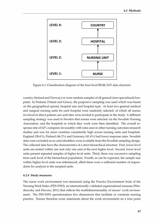
6.2 Methods
Figure 1. Classification diagram of the four-level RN4CAST data structure.
COUNTRY
NURSING UNIT
HOSPITAL
NURSE
LEVEL 4:
LEVEL 3:
LEVEL 2:
LEVEL 1:
Figure 6.1: Classification diagram of the four-level RN4CAST data structure
country (Ireland and Norway) or were random samples of all general (non-specialized) hos-pitals. In Finland, Poland and Greece, the purposive sampling was used which was basedon the geographical spread, hospital size and hospital type. At least two general medicaland surgical nursing units for each hospital were randomly selected, of which all nursesinvolved in direct patient care activities were invited to participate in the study. A differentsampling strategy was used in Sweden that nurses were selected via the Swedish NursingAssociation, and the hospitals in which they work were then identified. The overall re-sponse rate of 62% compares favourably with rates seen in other nursing outcomes researchstudies and was for most countries consistently high across nursing units and hospitals.England (38.6%), Finland (46.2%) and Germany (41.6%) had lower response rates. Swedishdata were excluded as no unit identifiers were available from the Swedish sampling design.The collected data have the characteristics of a strict hierarchical structure. First, lower levelunits are nested within one and only one unit at the next higher level. Second, lower levelunits present repeated samples of higher level units. Third, there was successive samplingfrom each level of the hierarchical population. Fourth, as can be expected, the sample sizewithin higher level units was imbalanced, albeit there were a sufficient number of respon-dents for analysis in the sampled units.
6.2.4 Study measures
The nurse work environment was measured using the Practice Environment Scale of theNursing Work Index (PES-NWI), an internationally validated organizational measure (War-shawsky and Havens, 2011) that reflects the multidimensionality of nurses’ work environ-ment. The PES-NWI operationalizes five dimensions that facilitate or constrain nursingpractice. Nurses therefore score statements about the work environment on a four point
87
Chapter 6 Group-level impact ... multilevel probit model
Likert scale (’Totally agree’=4, ’Agree’=3, ’Not agree’=2, ’Totally not agree’=1). The five di-mensions, example item and number of items of each dimension are: managerial supportfor nursing (’A nurse manager who is a good manager and leader’; 4 items), nurse participa-tion in hospital affairs (’Career development/clinical ladder opportunity’; 8 items), doctor-nurse collegial relations (’Physicians respect nurses as professionals’; 7 items), staffing andresource adequacy (’Enough registered nurses on staff to provide quality patient care’; 4items), and promotion of care quality (’Working with nurses who are clinically competent’; 9items). The Pearson coefficient correlation matrix showed relatively higher correlations be-tween the dimensions of staffing and resource adequacy and nurse participation in hospitalaffairs and other dimensions. This has the potential to adversely affect regression estimates.The multicollinearity checking showed a potential problem for the dimension nurse partic-ipation in hospital affairs. In addition, another paper by Kutney-Lee et al. (2009) used thesame three environment dimensions. We therefore did not include these two dimensionsfor further analyses.
The response variable for this analysis is the multidimensional burnout phenomenon.Burnout is a syndrome of emotional exhaustion, depersonalisation and reduced personalaccomplishment that can occur among individuals who do ”people work” of some kind(Maslach and Jackson, 1986). We evaluated burnout using the 22-item Maslach Burnout In-ventory (MBI) that has been extensively used to capture the three dimensions of burnout.On a seven point Likert scale, nurses assessed the frequency (ranging from never to everyday) of burnout experiences. Degrees of burnout are calculated separately for the dimen-sions of emotional exhaustion (9 items), depersonalisation (5 items) and reduced personalaccomplishment (8 items) by using the numerical cut-off points listed on Maslach and Jack-son (1986) scoring key. This key categorizes respondents into low, average and high rangesof experienced burnout for each dimension. We dichotomize respondents as experiencinghigh burnout or not, thus requiring a binary modelling. A probit regression was chosen inthis study.
About 10% of the nurses, at least one data value was missing on either the work envi-ronment or the burnout items. For the work environment dimensions, any missing datavalues were completed with the mean of the non-missing data values. For the dimensionsof burnout, missing data values were imputed using the multinomial distribution of fre-quencies per hospital. That is, each missing was replaced by a random value from theobserved multinomial distribution in each hospital. After applying the missing data impu-tation strategies in R (version 2.13.0), the final data set contained 23446 nurses coming from2087 nursing units, within 352 hospitals and 11 countries.
6.2.5 Statistical analysis
6.2.5.1 Intraclass Correlation Coefficient
The basic statistical prerequisite for the appropriate application of multilevel analyses in-cludes clustered data with a positive intraclass correlation coefficient (ICC). A (true) posi-tive ICC violates the independent observations assumption of ordinary least squares esti-
88
6.2 Methods
mation, resulting in downwardly biased standard error estimates, overly large test statistics,and inflated type I error rates (Krull and MacKinnon, 2001). We estimated the ICC to get anidea of the degree of variation in the burnout dimensions that were explained at each level.For the four-level model, the ICCs are defined as follows:
ICCc =σ2c
σ2all
, ICCh =σ2c + σ2
h
σ2all
, ICCh =σ2c + σ2
h + σ2u
σ2all
, (6.1)
with σ2all the sum of all variances, i.e. σ2
all = σ2c +σ2
h+σ2u+σ2
n . The subscripts c, h, u, n rep-resent country, hospital, nursing unit and nurse levels, respectively. For the probit model,the lowest level variance, i.e. σ2
n , is set to be one using the latent variable strategy. Regard-ing the interpretation of the intra-class correlation, we note that ICCc is the correlation oftwo nurses’ responses within the same country (different hospitals and nursing units), andICCh is the correlation of two nurses’ responses within the same hospital (same country butdifferent nursing units), while ICCu is the correlation of two nurses’ responses within thesame nursing unit (same country and hospital). The higher the ICC scores, the higher thedegree of homogeneity among nurses clusters. In order to get the partitioned proportion ofthe total variation into each level, we subtracted the higher level ICC from the lower levelICC, that is:
Pc =σ2c
σ2all
, Ph =σ2h
σ2all
, Pu =σ2u
σ2all
, Pn =σ2n
σ2all
. (6.2)
6.2.5.2 Model specification
The outcomes of interest, i.e. the three burnout subscales, take place at the individual level.These are called level-one outcomes. The work environment dimensions were conceptu-alized to influence these level-one outcomes at higher organizational levels. In multileveljargon, such variables are called ecological variables. We will continue to use this term andthe term work environment dimension throughout this paper. Contrary to previous nurseworkforce studies, we will avoid to name these variables environmental variables. Ecologi-cal variables were calculated as the average of the item responses of nurses within nursingunits, hospitals and countries. In a multilevel context, the effect of a covariate can be decom-posed into effects on different levels, which is recommended by Neuhaus and Kalbfleisch(1998). This decomposition allows us to learn the difference of the relationship at each level,which renders the modelling more flexible. We now rewrite each of the ecological variablesas follows:
Xu = (Xu − Xh) + (Xh − Xc) + Xc, (6.3)
where X is the aggregated average value of one of the work environment dimensions andthe subscripts u, h, c represent the nursing unit, hospital and country levels respectively.This representation partitions the nursing unit level covariate into a sum of three parts: thenursing unit level deviation from the hospital level mean, the hospital level deviation fromthe country level mean and the country level mean. The rationale is that, by partitioning
89
Chapter 6 Group-level impact ... multilevel probit model
the covariates we can estimate the pure effect of the covariate at each level. For example, bysubtracting the hospital level mean from the nursing unit level variable, we keep only theunit level effect thereby removing the higher level effects.
6.2.5.3 Step-by-step multilevel modelling approach
We propose a step-by-step approach towards building a model for multilevel regressionanalysis of the relationship between a multidimensional covariate and a multidimensionaldichotomous outcome. To relate the work environment dimensions to burnout dimensions,we first build a series of nine univariate simple multilevel probit models. Here, we con-sider the impact of each work environment dimension on each burnout dimension sep-arately. Second, we build a series of three univariate multiple multilevel probit models.Here, we consider the joint impact of the work environment dimensions on each of theburnout dimensions separately. The univariate simple multilevel probit model is describedin appendix A. The extension to the multiple model only involves adding more covariatesat each level.
The probit model assumes that there is an underlying latent variable Z that follows a nor-mal distribution with standard deviation one, conditional on all the fixed effects. This latentvariable expresses the true feeling of the nurse and is assumed that for Z > 0, burnout isexpressed on a manifest scale indicated by Y = 1, otherwise zero. In the univariate sim-ple multilevel probit models, we have one ecological covariate decomposed as in equation(3), augmented with a random intercept for each higher level. The random effects followa normal distribution with mean zero and a specific variance. No random slopes were in-cluded into the model following exploratory analyses (using Akaike’s information criterion(Akaike, 1974)), indicating that the relationship between the work environment and burnoutdiffers in different levels, but stays constant within each level. We used the same settingsfor the random effects in the univariate multiple multilevel probit models.
The final outcome of our step-by-step approach is a multivariate multilevel probit model.The combination of the three univariate multiple multilevel probit models results in a three-variate four-level probit model, which could also be called, in general, the multilevel mul-tivariate probit model (MVP) . In this modelling, a common factor was introduced to con-struct the correlations among the three burnout dimensions (cf. three-variate). Similar tothe univariate models, all three covariates are partitioned into three parts (unit, hospital,and country level pure effects). There are three random intercepts vectors corresponding tothe three higher levels for each outcome, as well as the three random factor loadings, whichimply a varying correlation structure. See appendix B for more details on the modelling ofmultilevel MVP.
6.2.5.4 Computational aspects
We used the R lme4 package (Bates et al., 2009) to fit the univariate simple and multiplemultilevel probit models. However, the multivariate multilevel probit model is beyond thescope of this package and we are not aware of any frequentist software that can handle this
90
6.3 Results
model. For this reason, we used the popular WinBUGS package. This software is based onthe Bayesian paradigm and uses Markov Chain Monte Carlo sampling techniques to arriveat the parameter estimates. A Bayesian analysis needs prior distributions for all its parame-ters. We have used here the following priors. For the regression coefficients we have takena normal distribution with mean zero and a large variance. The factor loadings (λs) weregiven a (multivariate) normal distribution with hyper-parameters, i.e. the variance (matrix),which has a vague conjugate inverse Wishart distribution. The random intercepts at eachlevel followed the same priors as the factor loadings. For the posterior statistics, we calcu-lated the posterior mean, median, standard error, and the 95% equal tail credibility interval.This credibility interval is the Bayesian equivalent of the classical 95% confidence interval,which indicates a significant non-zero estimate if the interval does not include zero, anda non-significant estimate if the interval includes zero. The hierarchical centering strategyof (Gelfand et al., 1995) was applied to improve the convergence of the MCMC iterations.Three chains were initialized with different starting values. We obtained posterior meansand 95% credible intervals based on 10,000 iterations after having removed a burn-in partof 20,000 iterations. The Brooks-Gelman-Rubin diagnostic plot (Brooks and Gelman, 1998),which tests the within- and between-chains variation, was used to check the convergence ofall parameters. The WinBUGS program is available from the first author.
6.3 Results
6.3.1 General description
The mean estimates of emotional exhaustion and depersonalisation burnout rates in Greeceare higher than for the other countries, while Poland has the highest rate of reduced per-sonal accomplishment. Greece shows the widest interquartile ranges for all three dimen-sions of burnout, while the Netherlands shows the narrowest. The burnout rates thus varygreatly across Greece hospitals but are stable across Dutch hospitals. Swiss nurses’ ratingsof their work environment are the highest for all three dimensions. Greek and Polish nurses’ratings of their work environment are lowest. The full descriptive findings were publishedpreviously by Aiken et al. (2012).
6.3.2 Intra-class Correlation Coefficients
Table 1 shows the proportion of total variance that could be explained at each level for thethree burnout dimensions and environment dimensions. The country level explained about22% of the variation in emotional exhaustion, 13% in depersonalisation and 6% in personalaccomplishment. The hospital level explains the least variation. Less than 5% in the vari-ation of all three outcomes can be explained at the hospital level. The nursing unit levelcontributes about 10%, 6% and 2% for the three outcomes respectively. These multilevelvariances decomposition indicate the modelling for multilevel analyses. For the variancesdecomposition of the three environment dimensions, the different proportions at each levelsuggest different ranges of the environment variations. The hospital level variation for each
91
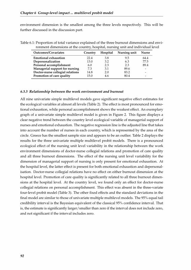
Chapter 6 Group-level impact ... multilevel probit model
environment dimension is the smallest among the three levels respectively. This will befurther discussed in the discussion part.
Table 6.1: Proportion of total variance explained of the three burnout dimensions and envi-ronment dimensions at the country, hospital, nursing unit and individual level
Outcomes/Covariates Country Hospital Nursing unit Nurse
Emotional exhaustion 22.4 3.8 9.5 64.4Depersonalization 13.0 3.2 6.3 77.5Personal accomplishment 6.0 2.3 2.3 89.4Managerial support for nursing 7.3 3.1 89.6 -Doctor-nurse collegial relations 14.8 2.0 83.2 -Promotion of care quality 15.0 4.6 80.4 -
6.3.3 Relationship between the work environment and burnout
All nine univariate simple multilevel models gave significant negative effect estimates forthe ecological variables at almost all levels (Table 2). The effect is most pronounced for emo-tional exhaustion, while personal accomplishment shows the weakest effect. An exemplarygraph of a univariate simple multilevel model is given in Figure 2. This figure displays aclear negative trend between the country level ecological variable of managerial support ofnurses and emotional exhaustion. The negative regression line is the adjusted line that takesinto account the number of nurses in each country, which is represented by the area of thecircle. Greece has the smallest sample size and appears to be an outlier. Table 2 displays theresults for the three univariate multiple multilevel probit models. There is a pronouncedecological effect of the nursing unit level variability in the relationship between the workenvironment dimensions of doctor-nurse collegial relations and promotion of care qualityand all three burnout dimensions. The effect of the nursing unit level variability for thedimension of managerial support of nursing is only present for emotional exhaustion. Atthe hospital level, the latter effect is present for both emotional exhaustion and depersonal-isation. Doctor-nurse collegial relations have no effect on either burnout dimension at thehospital level. Promotion of care quality is significantly related to all three burnout dimen-sions at the hospital level. At the country level, we found only an effect for doctor-nursecollegial relations on personal accomplishment. This effect was absent in the three-variatefour-level probit model (Table 3). The other fixed effects and the standard deviations in thefinal model are similar to those of univariate multiple multilevel models. The 95% equal tailcredibility interval is the Bayesian equivalent of the classical 95% confidence interval. Thatis, the estimate is significantly larger/smaller than zero if the interval does not include zero,and not significant if the interval includes zero.
92
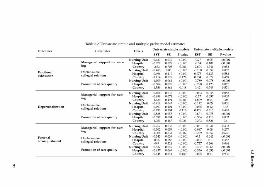
6.3R
esults
Table 6.2: Univariate simple and multiple probit model estimates
Outcomes Covariates Levels Univariate simple models Univariate multiple models
EST SE P-value EST SE P-value
Emotionalexhaustion
Managerial support for nurs-ing
Nursing Unit -0.623 0.039 <0.001 -0.27 0.05 <0.001Hospital -0.672 0.079 <0.001 -0.54 0.107 <0.001Country -2.33 0.708 0.001 -2.604 1.341 0.052
Doctor-nursecollegial relations
Nursing Unit -0.483 0.05 <0.001 -0.108 0.052 0.037Hospital -0.496 0.119 <0.001 0.073 0.133 0.582Country -1.114 0.729 0.126 0.634 0.877 0.469
Promotion of care qualityNursing Unit -1.109 0.061 <0.001 -0.789 0.078 <0.001
Hospital -0.684 0.097 <0.001 -0.298 0.125 0.017Country -1.559 0.661 0.018 -0.421 0.743 0.571
Depersonalization
Managerial support for nurs-ing
Nursing Unit -0.406 0.037 <0.001 -0.083 0.048 0.082Hospital -0.489 0.071 <0.001 -0.27 0.097 0.005Country -1.634 0.494 0.001 -1.839 0.94 0.05
Doctor-nursecollegial relations
Nursing Unit -0.419 0.047 <0.001 -0.172 0.05 0.001Hospital -0.493 0.104 <0.001 -0.085 0.12 0.48Country -0.793 0.504 0.116 0.429 0.615 0.485
Promotion of care qualityNursing Unit -0.838 0.058 <0.001 -0.671 0.075 <0.001
Hospital -0.597 0.084 <0.001 -0.354 0.113 0.002Country -1.081 0.467 0.021 -0.273 0.521 0.6
Personalaccomplishment
Managerial support for nurs-ing
Nursing Unit -0.257 0.032 <0.001 -0.031 0.041 0.453Hospital -0.302 0.059 <0.001 -0.087 0.08 0.277Country -1.008 0.331 0.002 -0.279 0.557 0.616
Doctor-nursecollegial relations
Nursing Unit -0.343 0.039 <0.001 -0.2 0.043 <0.001Hospital -0.35 0.085 <0.001 -0.087 0.1 0.387Country -0.9 0.228 <0.001 -0.727 0.364 0.046
Promotion of care qualityNursing Unit -0.537 0.049 <0.001 -0.407 0.065 <0.001
Hospital -0.437 0.069 <0.001 -0.336 0.093 <0.001Country -0.448 0.341 0.189 -0.025 0.31 0.936
93
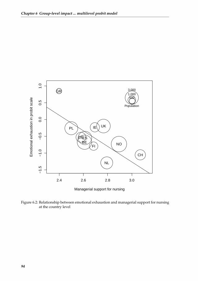
Chapter 6 Group-level impact ... multilevel probit model
2.4 2.6 2.8 3.0
−1.
5−
1.0
−0.
50.
00.
51.
0
Managerial support for nursing
Em
otio
nal e
xhau
stio
n in
pro
bit s
cale
●
BE
CH
DEES
FI
GR
IE
NL
NO
PL UK
●
3,0001,000500
Population
Figure 6.2: Relationship between emotional exhaustion and managerial support for nursingat the country level
94
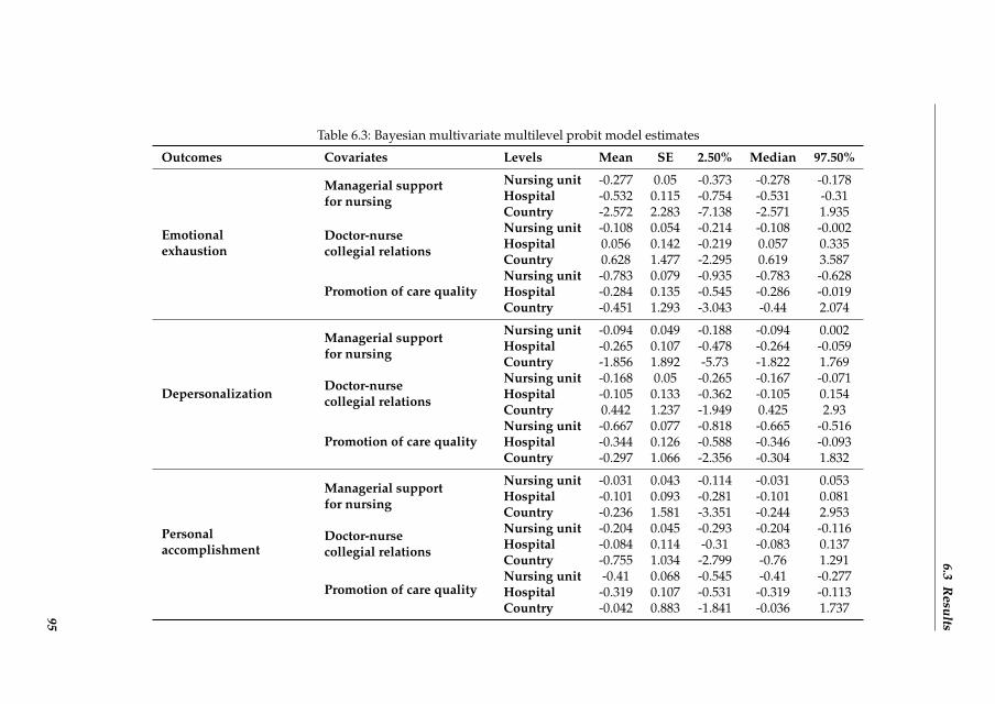
6.3R
esults
Table 6.3: Bayesian multivariate multilevel probit model estimates
Outcomes Covariates Levels Mean SE 2.50% Median 97.50%
Emotionalexhaustion
Managerial supportfor nursing
Nursing unit -0.277 0.05 -0.373 -0.278 -0.178Hospital -0.532 0.115 -0.754 -0.531 -0.31Country -2.572 2.283 -7.138 -2.571 1.935
Doctor-nursecollegial relations
Nursing unit -0.108 0.054 -0.214 -0.108 -0.002Hospital 0.056 0.142 -0.219 0.057 0.335Country 0.628 1.477 -2.295 0.619 3.587
Promotion of care qualityNursing unit -0.783 0.079 -0.935 -0.783 -0.628Hospital -0.284 0.135 -0.545 -0.286 -0.019Country -0.451 1.293 -3.043 -0.44 2.074
Depersonalization
Managerial supportfor nursing
Nursing unit -0.094 0.049 -0.188 -0.094 0.002Hospital -0.265 0.107 -0.478 -0.264 -0.059Country -1.856 1.892 -5.73 -1.822 1.769
Doctor-nursecollegial relations
Nursing unit -0.168 0.05 -0.265 -0.167 -0.071Hospital -0.105 0.133 -0.362 -0.105 0.154Country 0.442 1.237 -1.949 0.425 2.93
Promotion of care qualityNursing unit -0.667 0.077 -0.818 -0.665 -0.516Hospital -0.344 0.126 -0.588 -0.346 -0.093Country -0.297 1.066 -2.356 -0.304 1.832
Personalaccomplishment
Managerial supportfor nursing
Nursing unit -0.031 0.043 -0.114 -0.031 0.053Hospital -0.101 0.093 -0.281 -0.101 0.081Country -0.236 1.581 -3.351 -0.244 2.953
Doctor-nursecollegial relations
Nursing unit -0.204 0.045 -0.293 -0.204 -0.116Hospital -0.084 0.114 -0.31 -0.083 0.137Country -0.755 1.034 -2.799 -0.76 1.291
Promotion of care qualityNursing unit -0.41 0.068 -0.545 -0.41 -0.277Hospital -0.319 0.107 -0.531 -0.319 -0.113Country -0.042 0.883 -1.841 -0.036 1.73795
Chapter 6 Group-level impact ... multilevel probit model
6.3.4 Relationship among the burnout responses
Figure 3 displays the partitioned level-specific correlation structures among the three burnoutdimensions. The dots are the posterior means and the lines are the 95% confidence intervalin Bayesian way (for the country level or hospital level, this confidence interval is actuallythe median interval within the country or hospital). A sample of 20 is randomly selectedat hospital and nursing unit levels respectively to make the figure readable. At the countrylevel (first column in Figure 3), the correlations varied vastly, with some significant differ-ences between countries. At the hospital level (second column in Figure 3), all remainingcorrelation structures stayed close to zero after removing the country level correlations. Sim-ilar findings are seen for the nursing unit level after removing the country and hospital levelcorrelations (third column in Figure 3). This indicates that the correlation structure amongthe three outcomes was quite different between countries, but stayed stable between hospi-tals within countries and between nursing units within hospitals. Greece again performedmuch different from the other countries.
6.4 Discussion
In this paper, we investigated the relationship between nurse work environment dimen-sions (managerial support for nursing, doctor-nurse collegial relations, and promotion ofcare quality) and burnout dimensions (emotional exhaustion, depersonalisation, personalaccomplishment) using an advanced multilevel approach. We aimed to explore and investi-gate the effect of the nursing unit, hospital, and country level variability on the relationshipbetween dimensions of nurses’ work environment and dimensions of burnout. We also ex-plored the significance of the nursing unit, hospital, and country level variability among theburnout dimensions. We first specified ecological measures of the nurse work environmentdimensions at the three organizational levels (nursing unit, hospital, country). The effectof the covariate was decomposed into effects on different levels. This so called partitioningstrategy allowed us to specify the pure effect of the covariate at each level. We then com-bined these ecological measures with individual-level burnout experiences within a seriesof multilevel statistical models that would allow us to model the complex contextuality andheterogeneity.
Our approach towards building a model for multilevel regression analyses of the rela-tionship between such multidimensional covariate and multidimensional dichotomous out-come took three steps. We first fitted univariate simple multilevel probit models where weconsidered the impact of each work environment dimension on each burnout dimensionseparately. Second, we fitted univariate multiple multilevel probit models where we con-sidered the joint impact of the work environment dimensions on each of the burnout dimen-sions separately. Last, we fitted a multivariate multilevel probit model where we consideredthe joint impact of the work environment dimensions on the three burnout dimensions. Notsurprisingly, our results showed a negative relationship between work environment dimen-sions and burnout experiences among nurses. However, by maintaining in our advancedanalyses the social context in which the data were collected, we added some interesting
96

6.4 Discussion
Figure 3: Partitioned level-specific correlation structures among the three burnout
outcomes.a
correlation at country level
BelgiumSwitzerland
GermanySpain
FinlandGreeceIreland
the NetherlandsNorwayPoland
England
0.0 0.2 0.4 0.6
emotional exhaustion -- depersonalization
deviation of correlation at hospital level
-0.4 -0.2 0.0 0.2 0.4
deviation of correlation at unit level
-0.4 -0.2 0.0 0.2 0.4
correlation at country level
BelgiumSwitzerland
GermanySpain
FinlandGreeceIreland
the NetherlandsNorwayPoland
England
-0.4 -0.2 0.0 0.2 0.4
emotional exhaustion -- Personal accomplishment
deviation of correlation at hospital level
-0.4 -0.2 0.0 0.2 0.4
deviation of correlation at unit level
-0.4 -0.2 0.0 0.2 0.4
correlation at country level
BelgiumSwitzerland
GermanySpain
FinlandGreeceIreland
the NetherlandsNorwayPoland
England
-0.4 -0.2 0.0 0.2 0.4
depersonalization -- Personal accomplishment
deviation of correlation at hospital level
-0.4 -0.2 0.0 0.2 0.4
deviation of correlation at unit level
-0.4 -0.2 0.0 0.2 0.4
a For the hospital and nursing unit level deviation of correlations (the 2
nd and 3
rd columns), a
sample of 20 is randomly selected, respectively. Figure 6.3: Partitioned level-specific correlation structures among the three burnout out-
comes. For the hospital and nursing unit level deviation of correlations (the 2ndand 3rd columns), a sample of 20 is randomly selected, respectively.
97
Chapter 6 Group-level impact ... multilevel probit model
findings to what was already known about this relationship. By using the partition strat-egy and modelling the burnout and work environment dimensions jointly, we now have amore detailed view of their relationship. The final model showed no country-level effect foreither work environment dimension on any of the three burnout dimensions. Doctor-nursecollegial relations affected all burnout dimensions at the nursing unit level only. For the di-mension of promotion of care quality, the effect of the ecological exposure on burnout waspronounced at both the nursing unit and the hospital level for all three burnout dimensions.The magnitude of this effect was consistently stronger at the nursing unit. Findings for thedimension of managerial support for nursing were ambiguous. The effect on emotional ex-haustion was less pronounced at the nursing unit level than at the hospital level. An effecton depersonalization was only present at the hospital level. There was no effect on personalaccomplishment at either level. In developing the PES-NWI, Lake (2002) had already iden-tified that substantive domains of the subscales ranged from the broad hospital context tothe immediate nursing unit context, leading her to conclude that the subscales exhibit mul-tilevel range in hospital contexts. The varying magnitude in effects found at different levelsin this study pleas for the use of a multilevel analysis in future studies.
The results should however be interpreted with caution. Previous efforts from our re-search group have shown that aggregating features of nursing care of all nursing units atthe hospital level might obscure the hospital level effects on outcome measures (Van denHeede et al., 2009). For this study, that means that even though there is no hospital effectfor some work environment dimensions on certain burnout dimensions, human resourcesmanagement should not conclude that interventions at the hospital level are by definitionnot effective. Statistical support for this is given by the larger variance of work environmentand burnout dimensions at the unit than at the hospital level, as seen from the intraclass cor-relations (Table 1). The results indicate that all three work environment dimensions deservethe attention of human resources management to secure better outcomes. The pronouncedeffects of the dimensions of promotion of care quality and managerial support for nursesat both the nursing unit and the hospital level point to a need for leaders from bedsideto boardroom to further develop managerial skills and share goals for achieving positivehealth care environments. Front-line, middle and upper managers need to move towardsan integrated vision on promotion of care quality in tune with the workforce. As shownby our empirical findings, at the unit level, nurses should partner up with physicians. Themultivariate multilevel probit model allowed for a flexible hierarchical correlation struc-ture. We found a positive correlation matrix among the three burnout variables. This variedacross countries, but was stable across hospitals and nursing units within a specific country.
There is a large body of literature that has described the relationship between burnoutand work environment. Although some of them used different measure instruments, theycame up with similar findings. Melchior et al. (1997) analyzed the relationship betweenburnout and work environment at nurse level and nursing unit level separately. They foundsignificant relationships at each level. However, their modeling is not very efficient (sepa-rate analysis for each level) and suffers from a small sample size at the nursing unit level.Van Bogaert et al. (2009) explored the nursing unit level relationship between work envi-
98
6.4 Discussion
ronment dimensions and burnout using a 2-level linear mixed model for each of the threeburnout dimensions separately. They found significant relationships for all environmentcoefficients. O’Mahony (2011) studied the relationship between work environment and twoburnout dimensions (emotional exhaustion and depersonalization), and found a significantcorrelation through simple linear regressions. Liu et al. (2012) analyzed data from SouthChina using a logistic regression model and concluded that improving the unit level workenvironment from poor to better leads to a moderate (33%) decrease in job-related emo-tional exhaustion. As can be inferred in the results part, our 3-variate 4-level probit modeldetected similar findings as previous works at the nursing unit level. However, we providemore detailed information, also at higher levels, i.e. hospital and country levels.
Stepping back from what this article adds, it is not free from statistical, practical andconceptual limitations. First, we encountered multicollinearity between dimensions of thework environment. This multicollinearity could be due to specific items of different di-mensions correlating highly, rather than the whole dimensions. A confirmatory factor anal-ysis (CFA) is needed to study the factor structure underlying these items. The four-levelRN4CAST data structure would require a more complicated multilevel CFA to detect thepotentially different factor structure in each level. Such approach requires the applicationof new goodness-of-fit tests for verifying the statistical assumptions made at the differentlevels of the hierarchy. This analysis was beyond the scope of this study.
Second, the Bayesian multivariate multilevel probit model included no fixed effects inthe correlation structure among the three burnout dimensions, although adding covariatesis theoretically possible. In practice, such models with both fixed and random effects incorrelation structure causes rather slow convergence and needs to be improved further.
A third possible limitation is that country was treated as a random effect throughout thispaper. However, since country is not chosen at random (in contrast to hospital and nursingunit), we could have assumed that it has a fixed effect, involving an index variable for eachcountry.
In studies that involve multiple levels, researchers should be cautious of four types of fal-lacies that potentially arise when the methods fail to fit the conceptual model (Diez-Roux,1998). Ecological fallacies arise when drawing inferences at the individual level based ongroup-level data. Atomistic fallacies occur when drawing inferences at the group levelbased on individual level data. Ecological and atomistic fallacies are both types of infer-ential fallacies that can be overcome by ensuring that the data collected match the levelat which inferences are to be made, as was accomplished by the design of the RN4CASTproject. The psychological fallacy would arise when ignoring the relevant group-level co-variates in a study of individual level outcomes. In this article we have considered thenursing unit, hospital and country level variability in the relationship under study. Fourth,the sociological fallacy would arise when ignoring the role of individual level factors in astudy of groups. This brings us to a fourth potential limitation of the study. We have shownthat social contexts shape burnout experiences among nurses by including group-level vari-ables. By not including possible confounding individual level variables like nurses’ ageand gender, it might appear that we have perpetuated the idea that burnout experiences
99
Chapter 6 Group-level impact ... multilevel probit model
are absolutely socially determined rather than leaving room for individual determinants.Combining group-level and individual-level covariates in the proposed models is method-ologically challenging. It would be meaningful in future papers to analyze the joint impactof social context and individual characteristics on burnout experiences.
As described in the study sample section, the RN4CAST project accommodated withinthe framework of a strict hierarchy. A fifth potential limitation is that it is plausible that, al-though participating nurses strictly worked in the sampled nursing unit and hospital, bothcovariates and outcomes may be conditioned through social processes operating betweennursing units in hospitals.
Last, excluding Sweden from the final analysis may be considered misleading and ineffi-cient. We therefore did a sensitivity analysis to see the influence of the Swedish data on themodel estimates. These tests consist of three models which are: the hospital level univari-ate random effects model with country as the random effects, the country level univariateregression and the nurse level univariate random effects model with country and hospitalas the random effects. All these models were ran using both datasets with and withoutSwedish data to detect differing estimates. The difference was minimal, and the estimatesfrom the two data sets for all the three models were close, both for fixed and random effects.
6.5 Conclusions
Nurse work environment dynamics are related to nurses’ burnout experiences at both thenursing unit and the hospital level. The correlation structure among the three burnout out-comes varies across countries, but is stable between hospitals within countries and betweennursing units within hospitals. The findings provide a motivation for nurses and physi-cians within nursing units to partner up and for nurse leaders from bedside to boardroomto further develop their managerial skills. There is a clear need towards an integrated vi-sion on promotion of care quality in tune with the workforce. The results also imply that, inevaluating health care organizations, researchers should sample the different levels of theorganization under study and maintain this structure in analyzing the data.
References
Adewale, A. J., Hayduk, L., Estabrooks, C. A., Cummings, G. G., Midodzi, W. K., andDerksen, L. (2007). Understanding hierarchical linear models: Applications in nursingresearch. Nursing Research, 56(4):S40–S46.
Aiken, L. H., Clarke, S. P., Sloane, D. M., Sochalski, J. A., Busse, R., Clarke, H., Giovannetti,P., Hunt, J., Rafferty, A. M., and Shamian, J. (2001). Nurses reports on hospital care in fivecountries. Health Affairs, 20(3):43–53.
Aiken, L. H., Sermeus, W., Van den Heede, K., Sloane, D. M., Busse, R., McKee, M.,Bruyneel, L., Rafferty, A. M., Griffiths, P., Moreno-Casbas, M. T., et al. (2012). Patient safety,satisfaction, and quality of hospital care: Cross sectional surveys of nurses and patients in12 countries in Europe and the United States. BMJ: British Medical Journal, 344:e1717.
Akaike, H. (1974). A new look at the statistical model identification. Automatic Control,IEEE Transactions on, 19(6):716–723.
Bates, D., Maechler, M., and Ben, B. (2009). Package lme4.
100

References
Brooks, S. P. and Gelman, A. (1998). General methods for monitoring convergence of iter-ative simulations. Journal of Computational and Graphical Statistics, 7(4):434–455.
Bruyneel, L., den Heede, K. V., Diya, L., Aiken, L., and Sermeus, W. (2009). Predictivevalidity of the international hospital outcomes study questionnaire: An rn4cast pilot study.J Nurs Scholarsh, 41(2):202–210.
Cho, S.-H. (2003). Using multilevel analysis in patient and organizational outcomes re-search. Nursing Research, 52(1):61–65.
Diez-Roux, A. V. (1998). Bringing context back into epidemiology: Variables and fallaciesin multilevel analysis. American Journal of Public Health, 88(2):216–222.
Gajewski, B. J., Boyle, D. K., Miller, P. A., Oberhelman, F., and Dunton, N. (2010). A multi-level confirmatory factor analysis of the practice environment scale: A case study. NursingResearch, 59(2):147–153.
Gelfand, A., Sahu, S., and Carlin, B. (1995). Efficient parametrisations for normal linearmixed models. Biometrika, 82(3):479–488.
Hasselhorn, H., T. P. M. B. (2003). Working conditions and intent to leave the professionamong nursing staff in europe. Stockholm, National Institute for Working Life.
Kelly, L. A., McHugh, M. D., Aiken, L. H., et al. (2011). Nurse outcomes in magnet R© andnon-magnet hospitals. The Journal of Nursing Administration, 41(10):428.
Krull, J. L. and MacKinnon, D. P. (2001). Multilevel modeling of individual and group levelmediated effects. Multivariate Behavioral Research, 36(2):249–277.
Kutney-Lee, A., McHugh, M., Sloane, D., Cimiotti, J., Flynn, L., Neff, D., and Aiken, L.(2009). Nursing: A key to patient satisfaction. Health Affairs, 28(4):w669–w677.
Lake, E. T. (2002). Development of the practice environment scale of the nursing workindex. Res Nurs Health, 25(3):176–188.
Laschinger, H. K. S. and Leiter, M. P. (2006). The impact of nursing work environmentson patient safety outcomes: The mediating role of burnout engagement. Journal of NursingAdministration, 36(5):259–267.
Leiter, M. P. and Maslach, C. (2009). Nurse turnover: the mediating role of burnout. Journalof Nursing Management, 17(3):331–339.
Liu, K., You, L.-M., Chen, S.-X., Hao, Y.-T., Zhu, X.-W., Zhang, L.-F., and Aiken, L. H. (2012).The relationship between hospital work environment and nurse outcomes in guangdong,china: A nurse questionnaire survey. Journal of Clinical Nursing, 21(9-10):1476–1485.
Maslach, C. (1993). Burnout: A multidimensional perspective.
Maslach, C. and Jackson, S. E. (1986). Maslach burnout inventory. University of California,Palo Alto, CA.
Maslach, C., Jackson, S. E., and Leiter, M. P. (1996). Maslach Burnout Inventory Manual.Consulting Psychologists Pr, 3rd edition.
Maslach, C. and Leiter, M. P. (2008). Early predictors of job burnout and engagement.Journal of Applied Psychology, 93(3):498.
Melchior, M. E., van den Berg, A. A., Halfens, R., Abu-Saad, H. H., Philipsen, H., andGassman, P. (1997). Burnout and the work environment of nurses in psychiatric long-staycare settings. Soc Psychiatry Psychiatr Epidemiol, 32(3):158–164.
Nantsupawat, A., Srisuphan, W., Kunaviktikul, W., Wichaikhum, O.-A., Aungsuroch, Y.,and Aiken, L. H. (2011). Impact of nurse work environment and staffing on hospital nurseand quality of care in thailand. Journal of Nursing Scholarship, 43(4):426–432.
101
Chapter 6 Group-level impact ... multilevel probit model
Neuhaus, J. M. and Kalbfleisch, J. D. (1998). Between- and within-cluster covariate effectsin the analysis of clustered data. Biometrics, 54(2):638–645.
O’Mahony, N. (2011). Nurse burnout and the working environment. Emerg Nurse, 19(5):30–37.
Park, S. and Lake, E. T. (2005). Multilevel modeling of a clustered continuous outcome:Nurses’ work hours and burnout. Nursing research, 54(6):406.
Poghosyan, L., Aiken, L. H., and Sloane, D. M. (2009). Factor structure of the maslachburnout inventory: An analysis of data from large scale cross-sectional surveys of nursesfrom eight countries. Int J Nurs Stud, 46(7):894–902.
Sermeus, W., Aiken, L. H., den Heede, K. V., Rafferty, A. M., Griffiths, P., Moreno-Casbas,M. T., Busse, R., Lindqvist, R., Scott, A. P., Bruyneel, L., Brzostek, T., Kinnunen, J., Schubert,M., Schoonhoven, L., Zikos, D., and consortium, R. N. A. S. T. (2011). Nurse forecasting ineurope (rn4cast): Rationale, design and methodology. BMC Nurs, 10:6.
Vahey, D., Aiken, L., Sloane, D., Clarke, S., and Vargas, D. (2004). Nurse burnout andpatient satisfaction. Medical Care, 42(2 Suppl):II57.
Van Bogaert, P., Meulemans, H., Clarke, S., Vermeyen, K., and Van de Heyning, P. (2009).Hospital nurse practice environment, burnout, job outcomes and quality of care: Test of astructural equation model. Journal of Advanced Nursing, 65(10):2175–2185.
Van den Heede, K., Lesaffre, E., Diya, L., Vleugels, A., Clarke, S. P., Aiken, L. H., and Ser-meus, W. (2009). The relationship between inpatient cardiac surgery mortality and nursenumbers and educational level: Analysis of administrative data. International Journal ofNursing Studies, 46(6):796–803.
Warshawsky, N. E. and Havens, D. S. (2011). Global use of the practice environment scaleof the nursing work index. Nursing Research, 60(1):17.
Wu, Y.-W. B. (1997). An application of hierarchical linear models to meta-analysis in nurs-ing research. Nursing Research, 46(5):295–298.
102
Appendix
Appendix
A. Univariate simple multilevel probit model
Let Znuhc be one of the three latent normally distributed responses, representing the nthnurse, within the uth nursing unit, the hth hospital and the cth country. This variable ex-presses the true burnout feeling of the nurse. It is assumed that for Znuhc > 0, burnout isexpressed on a manifest scale indicated by Ynuhc = 1, otherwise 0.
Znuhc = β0 + β1Xuhc + β2Xhc + β3Xc + b0c + b0hc + b0uhc + εnuhc
b0c ∼ N(0, σ21), b0hc ∼ N(0, σ2
2), b0uhc ∼ N(0, σ23), εnuhc ∼ N(0, 1),
n = 1, 2, ..., Nu, u = 1, 2, ..., Nh, h = 1, 2, ..., Nc, c = 1, 2, ..., 11
(6.4)
B. Multivariate multilevel probit model
For a better understanding, we first introduce the classical multivariate probit model (MVP)(single-level structure). The classical MVP has been widely studied by many researcherswith different theories and solutions, see e.g. Bock and Gibbons (1996), Chib and Greenberg(1998), Lawrence et al. (2008). Here we adopt Bock and Gibbons’ solution of factor modllingwhich is formally defined as follows:
Zi = β0 + β1Xi + λ0Fi + εi,
Fi ∼ N(0, 1), εi ∼ N(0,Σε), i = 1, 2, ..., N,(6.5)
where in our three-variate case, Zi is a 3× 1 vector of latent continuous responses at the ithobservation, with the same definition of latent variable as in the univariate case. The vectorsof regression coefficients β0 and β1 , and the vector of factor loadings λ0 are of length 3,corresponding to the three outcomes. The common factor Fi serves to model the correlationsof the three outcomes in combination with the covariance structure of the residuals εi , Σε
. We assumed that this covariance matrix is diagonal (errors independent). The covariancematrix of the random part, i.e. cov(λ0Fi + εi) = λ0λ
T0 + Σε , is called the factor analytic
representation of the covariance which can reproduce any 3×3 covariance matrix by anappropriate choice of λ0 and Σε . Note that here the covariance matrix equals the correlationmatrix because the variances are assumed to be one. This model assumes that the correlationmatrix is the same across all countries, hospitals and nursing units, which might be not arealistic assumption. In order to vary the correlation across countries one could replace λ0Fi
by (λ0 +λc)Fi , whereby λc changes with country. In this way there are as many correlationmatrices as countries. We can further extend this expression to let the correlation vary alsowith hospital and nursing unit resulting in a term (λ0 + λc + λhc + λuhc)Fnuhc. In this waywe have a different correlation matrix for each nursing unit. Because of the large number
103
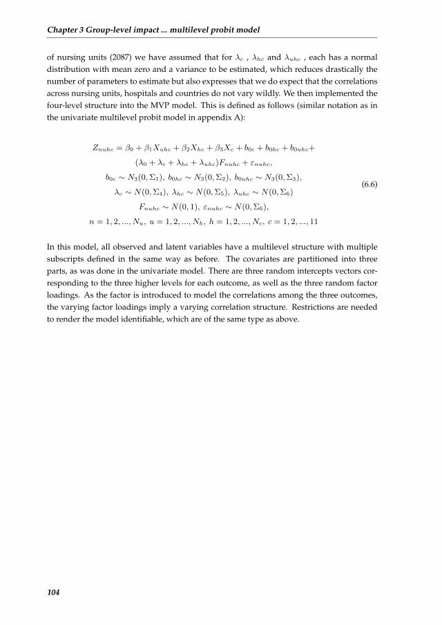
Chapter 3 Group-level impact ... multilevel probit model
of nursing units (2087) we have assumed that for λc , λhc and λuhc , each has a normaldistribution with mean zero and a variance to be estimated, which reduces drastically thenumber of parameters to estimate but also expresses that we do expect that the correlationsacross nursing units, hospitals and countries do not vary wildly. We then implemented thefour-level structure into the MVP model. This is defined as follows (similar notation as inthe univariate multilevel probit model in appendix A):
Znuhc = β0 + β1Xuhc + β2Xhc + β3Xc + b0c + b0hc + b0uhc+
(λ0 + λc + λhc + λuhc)Fnuhc + εnuhc,
b0c ∼ N3(0,Σ1), b0hc ∼ N3(0,Σ2), b0uhc ∼ N3(0,Σ3),
λc ∼ N(0,Σ4), λhc ∼ N(0,Σ5), λuhc ∼ N(0,Σ6)
Fnuhc ∼ N(0, 1), εnuhc ∼ N(0,Σ6),
n = 1, 2, ..., Nu, u = 1, 2, ..., Nh, h = 1, 2, ..., Nc, c = 1, 2, ..., 11
(6.6)
In this model, all observed and latent variables have a multilevel structure with multiplesubscripts defined in the same way as before. The covariates are partitioned into threeparts, as was done in the univariate model. There are three random intercepts vectors cor-responding to the three higher levels for each outcome, as well as the three random factorloadings. As the factor is introduced to model the correlations among the three outcomes,the varying factor loadings imply a varying correlation structure. Restrictions are neededto render the model identifiable, which are of the same type as above.
104
7A MULTIVARIATE MULTILEVEL
GAUSSIAN MODEL WITH A MIXEDEFFECTS STRUCTURE IN THE MEAN
AND COVARIANCE PART
Chapter 7 is based on the paper:Li, B., Bruyneel, L., and Lesaffre, E. (2014). A multivariate multilevel Gaussian model with a mixedeffects structure in the mean and covariance part. Statistics in Medicine. 33(11):1877-1899.
105
Chapter 7 A multivariate multilevel ... mean and covariance part
Abstract
A traditional Gaussian hierarchical model assumes a nested multilevelstructure for the mean and a constant variance at each level. We proposea Bayesian multivariate multilevel factor model that assumes a multi-level structure for both the mean and the covariance matrix. That is, inaddition to a multilevel structure for the mean we also assume that thecovariance matrix depends on covariates and random effects. This al-lows to explore whether the covariance structure depends on the valuesof the higher levels and as such models heterogeneity in the variancesand correlation structure of the multivariate outcome across the higherlevel values. The approach is applied to the three-dimensional vector ofburnout measurements collected on nurses in a large European study toanswer the research question whether the covariance matrix of the out-comes depends on recorded system-level features in the organization ofnursing care, but also on not-recorded factors that vary with countries,hospitals and nursing units. Simulations illustrate the performance ofour modeling approach.
106

7.1 Introduction
7.1 Introduction
In this paper we are interested in modeling a multivariate multilevel Gaussian data struc-ture. Our modeling approach is inspired by research questions that were formulated in thecontext of the Registered Nurse Forecasting (RN4CAST) project (Sermeus et al., 2011). ThisEuropean FP7-funded nurse workforce study was conducted from 2009 to 2011 in twelvecountries in Europe and involved a large number of hospitals, nursing units and nurses.The aim of the project was to study the impact of system-level features in the organizationof nursing care (work environment, educational level, workload) on individual measuresof nurse wellbeing (burnout, job satisfaction, turnover) and patient safety outcomes andsatisfaction with care. As outcome we have chosen three classically used burnout scoresdeveloped about twenty years ago in the US from a 22-item questionnaire (Maslach et al.,1996). These scores have been used intensively in the nursing research literature and areperceived to represent well the burnout process.
It was of interest to know how each of the burnout outcomes depend on country, hospi-tal, nursing unit and nurse characteristics. Such dependencies can be explored by fitting amultilevel model to each of the three outcomes. However such a model only explores thedependence of the mean on the covariates. It is equally important to see whether these fac-tors also impact the variability of burnout. Indeed a high variability of burnout within, saya hospital, may also affect the quality of care in that hospital. Furthermore, we were curiouswhether the relationship of the three burnout outcomes remained constant across the valuesof the different levels of the multilevel structure. In particular we were interested in lookingfor factors that alter the correlation structure of the burnout measurements. Such determi-nants may shed light on whether the dimensions of burnout vary with covariates. Finally,it is important to realize that in the RN4CAST study, the 22-item questionnaire was trans-lated into eleven languages. Although translation was done by experts, it may still happenthat the interpretation of the questions depends on local, say ethnic or cultural, differences.Since no information on such factors was recorded in the RN4CAST study, we wished toexplore the variability of the correlation structure of the burnout outcomes across the dif-ferent levels of the data. To explore the dependence of the covariance matrix on recordedand not-recorded covariates we propose here to extend the classical multivariate multilevelmodel with a covariance matrix that may depend on covariates and random effects.
For the 2-level model, various approaches were suggested in the literature to allow thevariance function of the random effect and/or of measurement error to depend on covari-ates, see e.g. Ibanez et al. (1999); Foulley et al. (1990); Lin et al. (1997). Approaches werealso suggested whereby the variance structure contains random effects. Foulley et al. (1992)proposed a Bayesian linear mixed model whereby the measurement error variance also hasa mixed model structure. Foulley and Gianola (1996) then further extended this model togeneralized linear mixed models. Kizilkaya and Tempelman (2005) applied a full Bayesianstructural mixed effects multiplicative model for residual variances in a generalized linearmixed model. Lee and Nelder (2006) proposed a DHGLM (Double Hierarchical General-ized Linear Model), which models both mean and the residual variance (overdispersion)
107

Chapter 7 A multivariate multilevel ... mean and covariance part
with random effects. Further, Lee and Noh (2012) extended the DHGLM to model mean,residual variance, and also variance of random effects, with random effects.
For a multivariate Gaussian response, extensions of the classical regression model havebeen suggested whereby the covariance matrix is allowed to depend on covariates. In thisrespect, one may model the covariance matrix directly as a function of covariates or firstsplit up the covariance matrix into the correlation and variance part and model both partsseparately. The major challenge is to ensure that the covariance matrix remains positivedefinite for all covariate values. Chiu et al. (1996) proposed a way of directly modelingthe logarithmic transformation of the covariance matrix. Although it is a flexible approachwithout causing positive definite problems, the interpretation of the model parameters isoften quite difficult. A popular approach was suggested by Pourahmadi (1999) who usedthe separation strategy and suggested a modified Cholesky decomposition of the covari-ance matrix, i.e. TΣTT = D, and then modeled the elements of T and D as a function ofcovariates. The interpretation of the parameters is meaningful, however, only when thereexists a natural ranking of the responses as in longitudinal studies or time series studies.For applications of this approach, see e.g. Daniels and Pourahmadi (2002) and Cecere et al.(2006). Barnard et al. (2000) suggested another decomposition which separates the covari-ance matrix into the (classical) variance and correlation part, i.e. Σ = diag(S)Rdiag(S). Italso allows for heterogeneous covariance matrices across groups, e.g. gender or age groups.The computation, however, is intensive for moderate and large sample size. More recently,Hoff and Niu (2012) proposed a covariance regression model to allow for heterogeneity inthe variance part of the classic multivariate regression model. They suggested the modelΣx = A + BxxTBT , whereby A is a “baseline” positive definite matrix and B a matrixof regression coefficients. Fox and Dunson (2011) suggested a Bayesian non-parametric co-variance regression that could efficiently reduce the high parameter dimensionality, whichis especially useful when the dimensionality of response is high.
For multivariate multilevel models, the literature lacks modeling approaches that allowthe covariance matrix to depend on covariates and/or random effects. In this paper wegeneralized the approach of Hoff and Niu by specifying a factor analytic model to the three-dimensional response with the factor loadings depending on covariates and random effects.The covariance matrix could then be built up through the factor loadings to have a complexstructure. This somewhat resembles structural equation modeling (SEM) which aims at 1)understand the patterns of covariances among a set of observed variables and 2) explain asmuch of their variance as possible with the researcher’s model (Kline, 2010). The differenceof our approach with SEM will be discussed at the end.
In Section 7.2 we provide further details on the motivating data set and introduce theresearch questions that triggered our modeling approach(es). In Section 7.3 we elaborateon a factor-analytic approach to model the covariance matrix in a hierarchical way. Bothcovariates as well as random effects are incorporated into the covariance structure. In Sec-tion 7.4 we indicate how our approach can be generalized to more than three responses.The MCMC procedure to estimate the model parameters is discussed in Section 7.5. Section7.6 focuses on the impact of the non-response issue and the handling of missingness in the
108

7.2 Motivating data set: the RN4CAST project
response and the covariates. In Section 7.7 the multivariate multilevel model is applied tothe motivating RN4CAST data set and the research questions posed in Section 7.2 are ad-dressed. Simulation studies to illustrate the performance of our modeling approach(es) aredescribed in Section 7.8. We give concluding remarks in Section 7.9.
7.2 Motivating data set: the RN4CAST project
7.2.1 Description of the project
The RN4CAST project is a three year (2009-2011) nurse workforce study involving 33731registered nurses in 2169 nursing units in 486 hospitals in 12 European countries. Multi-level sampling was conducted such that within each of the 12 countries, a minimum of 30general (non-specialized) hospitals were randomly selected, except for Ireland and Norwaywhere the selected hospitals represented all of the relevant institutions. At least two adultgeneral medical and surgical nursing units for each hospital were randomly selected, sincethe link of nurses’ workload and work environment to patient safety and clinical outcomesis best documented in these types of nursing units. All nurses involved in direct patient careactivities were then invited to the study. The overall response rate was 62%. While thereis a considerable non-response rate, it compares favorably with rates seen in other nursingoutcomes research studies of this scale (Aiken et al., 2002). Hospital level response rates ex-ceeded 50% for all countries except for Greece (42%) and the Netherlands (37%). All nursingunits that were randomly selected within the participating hospitals agreed to participate tothe study. Individual nurse response rates across countries were consistently high, exceptfor England (38.6%), Finland (46.2%) and Germany (41.6%). Swedish data were excludedas no unit identifiers were available from the Swedish sampling design. For more detailson the sampling strategy, see Sermeus et al. (2011). In Section 7.6 we return to the possibleimpact of the non-response on scientific conclusions from the RN4CAST study.
Burnout was measured using the 22-item Maslach Burnout Inventory (MBI) with eachitem having a seven-point Likert scale (from never to every day coded from 0 to 6) on thefrequency of burnout experiences, e.g. ”I feel emotionally drained from my work”. Maslachet al. (1996) extracted three main dimensions of burnout: emotional exhaustion (EE), deper-sonalization (DP) and reduced personal accomplishment (PA). These three dimensions are sumscores obtained from the original MBI scale. There are about 10% of the nurses having atleast one of the 22 items missing. In Section 7.6 we elaborate on how we dealt with the miss-ing part in the response. Burnout is indicated by higher scores on EE and DP, and lowerscores on PA, but we reversed the code for PA for interpretational purposes (for the threeburnout measurements a large value means then more burnout). The crude correlationsamong these dimensions are 0.56 for EE and DP, 0.28 for EE and PA, and 0.32 for DP andPA, somewhat higher than 0.52, 0.22 (reversed) and 0.26 (reversed), as reported by Maslachet al. (1996). It is assumed in the literature that the three dimensions describe relatively wellburnout.
The survey battery including the MBI was translated into eleven languages from its origi-nal American English version while ensuring its relevance to the nursing practice and health
109
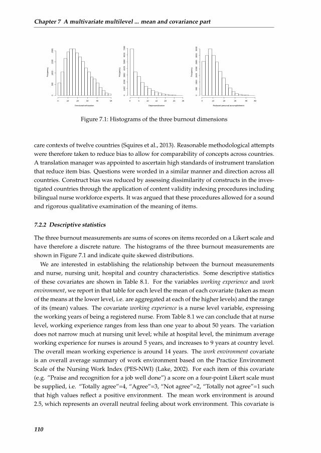
Chapter 7 A multivariate multilevel ... mean and covariance part
Emotional exhaustion
Fre
quen
cy
0 10 20 30 40 54
050
010
0015
0020
00
Depersonalization
Fre
quen
cy
0 5 10 15 20 25 30
010
0020
0030
0040
0050
0060
0070
00
Reduced personal accomplishment
Fre
quen
cy
0 10 20 30 40 48
050
010
0015
0020
0025
0030
0035
00
Figure 7.1: Histograms of the three burnout dimensions
care contexts of twelve countries (Squires et al., 2013). Reasonable methodological attemptswere therefore taken to reduce bias to allow for comparability of concepts across countries.A translation manager was appointed to ascertain high standards of instrument translationthat reduce item bias. Questions were worded in a similar manner and direction across allcountries. Construct bias was reduced by assessing dissimilarity of constructs in the inves-tigated countries through the application of content validity indexing procedures includingbilingual nurse workforce experts. It was argued that these procedures allowed for a soundand rigorous qualitative examination of the meaning of items.
7.2.2 Descriptive statistics
The three burnout measurements are sums of scores on items recorded on a Likert scale andhave therefore a discrete nature. The histograms of the three burnout measurements areshown in Figure 7.1 and indicate quite skewed distributions.
We are interested in establishing the relationship between the burnout measurementsand nurse, nursing unit, hospital and country characteristics. Some descriptive statisticsof these covariates are shown in Table 8.1. For the variables working experience and workenvironment, we report in that table for each level the mean of each covariate (taken as meanof the means at the lower level, i.e. are aggregated at each of the higher levels) and the rangeof its (mean) values. The covariate working experience is a nurse level variable, expressingthe working years of being a registered nurse. From Table 8.1 we can conclude that at nurselevel, working experience ranges from less than one year to about 50 years. The variationdoes not narrow much at nursing unit level; while at hospital level, the minimum averageworking experience for nurses is around 5 years, and increases to 9 years at country level.The overall mean working experience is around 14 years. The work environment covariateis an overall average summary of work environment based on the Practice EnvironmentScale of the Nursing Work Index (PES-NWI) (Lake, 2002). For each item of this covariate(e.g. ”Praise and recognition for a job well done”) a score on a four-point Likert scale mustbe supplied, i.e. “Totally agree”=4, “Agree”=3, “Not agree”=2, “Totally not agree”=1 suchthat high values reflect a positive environment. The mean work environment is around2.5, which represents an overall neutral feeling about work environment. This covariate is
110

7.2 Motivating data set: the RN4CAST project
quite stable across countries but varies more across nurses and nursing units. The covariatesize represents the total number of beds at hospital level (varying from 30 to 3,000) and thenumber of participating nurses at the nursing unit level (varying between 1 and 80). Thetype of hospital and type of nursing unit appear to play a role for burnout (Servellen andLeake, 1993) and are therefore considered here as possible factors that influence burnout.We considered two hospital characteristics: teaching status (a university hospital = 1, or not= 0) and technology level (heart surgery and/or transplant surgery available = 1, or not = 0).These two types of hospitals constitute around 24% and 29% of all hospitals, respectively.The nursing units were classified as either surgical (about 50%) or medical, whereby around4.7% of the nursing units recorded as both surgical and medical were classified as medical.
Working experience was not reported for about 6.3% of the nurses. For the other covari-ates there was less than 2% missing. In Section 7.6 we detail on how we treated the missingcovariate values. Finally, there were only 7% male nurses and burnout might be stronglyrelated to gender, we preferred to consider a more homogeneous group and restricted ouranalysis to the female nurses. As a result, Table 8.1 is based on 21016 nurses, coming from2023 nursing units within 345 hospitals in 11 countries.
Table 7.1: Descriptive statistics of the considered covariates in the statistical models.
Working exp- Work env-Size∗†
Teaching Technical Surgery n-erience(yrs)∗ ironment∗ hospital‡ hospital‡ ursing unit‡
Country 13.9 (9.1,18.8) 2.5 (2.3,2.9) – – – –Hospital 14.3 (5.1,27.8) 2.5 (1.7,3.3) 483.6 (30,3213) 23.8% 29.0% –Nursing unit13.9 (0.3,41.0) 2.5 (1.4,3.6) 11.4 (1,71) – – 49.9%Nurse 13.9 (0.1,50.0) – – – – –∗: Mean (and range)†: No. of beds at hospital level and No. of available nurses at nursing unit level‡: Percentage
7.2.3 Research questions
The following research questions regarding burnout among nurses emerged:
• Question 1: How much variability does each of the three burnout measurements showacross countries, hospitals (within countries), nursing units (within countries and hos-pitals) and nurses (within countries, hospitals and nursing units)?
• Question 2: How much of the variability can be explained with the covariates recordedat the different levels?
• Question 3: Does the covariance matrix (and more precisely the correlation) betweenthe three burnout dimensions remain the same across countries, hospitals, nursing
111
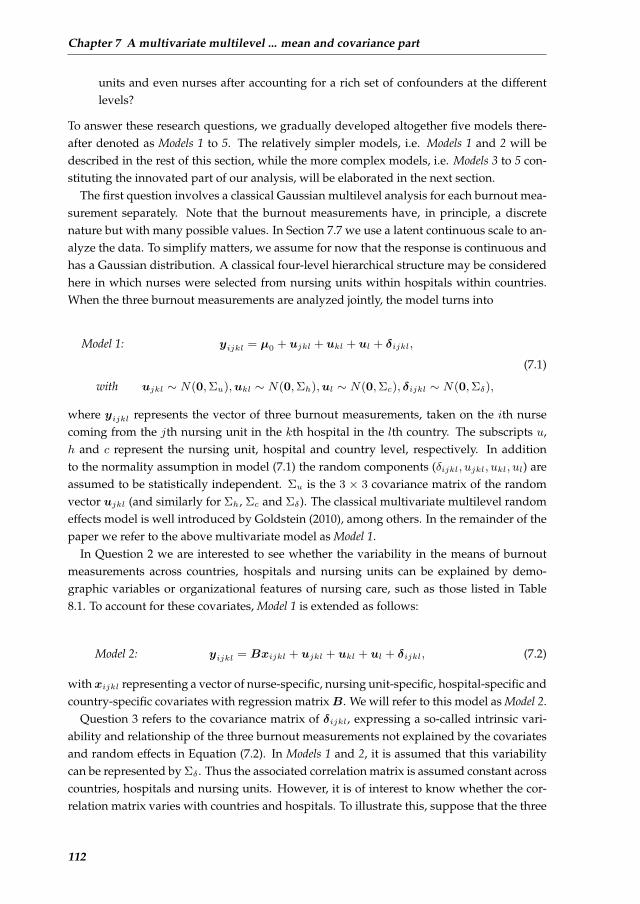
Chapter 7 A multivariate multilevel ... mean and covariance part
units and even nurses after accounting for a rich set of confounders at the differentlevels?
To answer these research questions, we gradually developed altogether five models there-after denoted as Models 1 to 5. The relatively simpler models, i.e. Models 1 and 2 will bedescribed in the rest of this section, while the more complex models, i.e. Models 3 to 5 con-stituting the innovated part of our analysis, will be elaborated in the next section.
The first question involves a classical Gaussian multilevel analysis for each burnout mea-surement separately. Note that the burnout measurements have, in principle, a discretenature but with many possible values. In Section 7.7 we use a latent continuous scale to an-alyze the data. To simplify matters, we assume for now that the response is continuous andhas a Gaussian distribution. A classical four-level hierarchical structure may be consideredhere in which nurses were selected from nursing units within hospitals within countries.When the three burnout measurements are analyzed jointly, the model turns into
Model 1: yijkl = µ0 + ujkl + ukl + ul + δijkl,
with ujkl ∼ N(0,Σu),ukl ∼ N(0,Σh),ul ∼ N(0,Σc), δijkl ∼ N(0,Σδ),
(7.1)
where yijkl represents the vector of three burnout measurements, taken on the ith nursecoming from the jth nursing unit in the kth hospital in the lth country. The subscripts u,h and c represent the nursing unit, hospital and country level, respectively. In additionto the normality assumption in model (7.1) the random components (δijkl, ujkl, ukl, ul) areassumed to be statistically independent. Σu is the 3 × 3 covariance matrix of the randomvector ujkl (and similarly for Σh, Σc and Σδ). The classical multivariate multilevel randomeffects model is well introduced by Goldstein (2010), among others. In the remainder of thepaper we refer to the above multivariate model as Model 1.
In Question 2 we are interested to see whether the variability in the means of burnoutmeasurements across countries, hospitals and nursing units can be explained by demo-graphic variables or organizational features of nursing care, such as those listed in Table8.1. To account for these covariates, Model 1 is extended as follows:
Model 2: yijkl = Bxijkl + ujkl + ukl + ul + δijkl, (7.2)
withxijkl representing a vector of nurse-specific, nursing unit-specific, hospital-specific andcountry-specific covariates with regression matrixB. We will refer to this model as Model 2.
Question 3 refers to the covariance matrix of δijkl, expressing a so-called intrinsic vari-ability and relationship of the three burnout measurements not explained by the covariatesand random effects in Equation (7.2). In Models 1 and 2, it is assumed that this variabilitycan be represented by Σδ . Thus the associated correlation matrix is assumed constant acrosscountries, hospitals and nursing units. However, it is of interest to know whether the cor-relation matrix varies with countries and hospitals. To illustrate this, suppose that the three
112
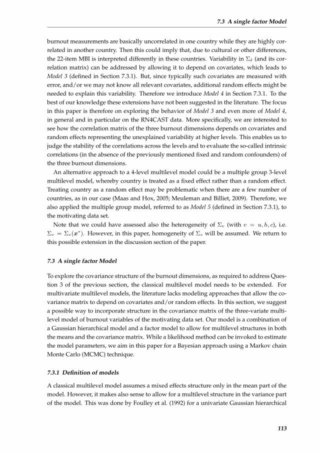
7.3 A single factor Model
burnout measurements are basically uncorrelated in one country while they are highly cor-related in another country. Then this could imply that, due to cultural or other differences,the 22-item MBI is interpreted differently in these countries. Variability in Σδ (and its cor-relation matrix) can be addressed by allowing it to depend on covariates, which leads toModel 3 (defined in Section 7.3.1). But, since typically such covariates are measured witherror, and/or we may not know all relevant covariates, additional random effects might beneeded to explain this variability. Therefore we introduce Model 4 in Section 7.3.1. To thebest of our knowledge these extensions have not been suggested in the literature. The focusin this paper is therefore on exploring the behavior of Model 3 and even more of Model 4,in general and in particular on the RN4CAST data. More specifically, we are interested tosee how the correlation matrix of the three burnout dimensions depends on covariates andrandom effects representing the unexplained variability at higher levels. This enables us tojudge the stability of the correlations across the levels and to evaluate the so-called intrinsiccorrelations (in the absence of the previously mentioned fixed and random confounders) ofthe three burnout dimensions.
An alternative approach to a 4-level multilevel model could be a multiple group 3-levelmultilevel model, whereby country is treated as a fixed effect rather than a random effect.Treating country as a random effect may be problematic when there are a few number ofcountries, as in our case (Maas and Hox, 2005; Meuleman and Billiet, 2009). Therefore, wealso applied the multiple group model, referred to as Model 5 (defined in Section 7.3.1), tothe motivating data set.
Note that we could have assessed also the heterogeneity of Σv (with v = u, h, c), i.e.Σv = Σv(x∗). However, in this paper, homogeneity of Σv will be assumed. We return tothis possible extension in the discussion section of the paper.
7.3 A single factor Model
To explore the covariance structure of the burnout dimensions, as required to address Ques-tion 3 of the previous section, the classical multilevel model needs to be extended. Formultivariate multilevel models, the literature lacks modeling approaches that allow the co-variance matrix to depend on covariates and/or random effects. In this section, we suggesta possible way to incorporate structure in the covariance matrix of the three-variate multi-level model of burnout variables of the motivating data set. Our model is a combination ofa Gaussian hierarchical model and a factor model to allow for multilevel structures in boththe means and the covariance matrix. While a likelihood method can be invoked to estimatethe model parameters, we aim in this paper for a Bayesian approach using a Markov chainMonte Carlo (MCMC) technique.
7.3.1 Definition of models
A classical multilevel model assumes a mixed effects structure only in the mean part of themodel. However, it makes also sense to allow for a multilevel structure in the variance partof the model. This was done by Foulley et al. (1992) for a univariate Gaussian hierarchical
113
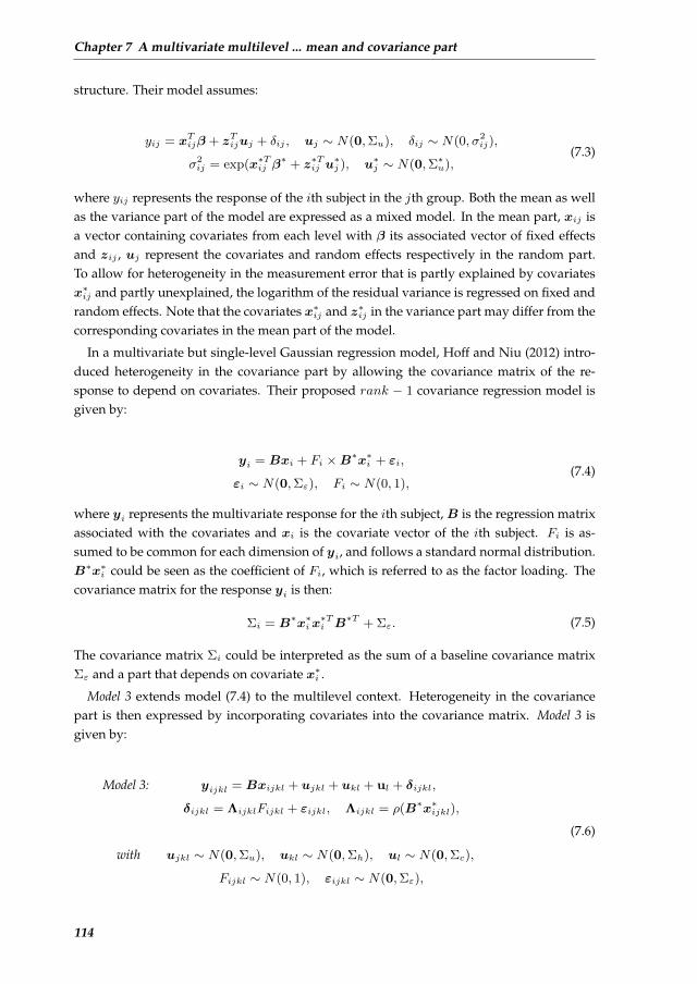
Chapter 7 A multivariate multilevel ... mean and covariance part
structure. Their model assumes:
yij = xTijβ + zTijuj + δij , uj ∼ N(0,Σu), δij ∼ N(0, σ2ij),
σ2ij = exp(x∗Tij β
∗ + z∗Tij u∗j ), u∗j ∼ N(0,Σ∗u),
(7.3)
where yij represents the response of the ith subject in the jth group. Both the mean as wellas the variance part of the model are expressed as a mixed model. In the mean part, xij isa vector containing covariates from each level with β its associated vector of fixed effectsand zij , uj represent the covariates and random effects respectively in the random part.To allow for heterogeneity in the measurement error that is partly explained by covariatesx∗ij and partly unexplained, the logarithm of the residual variance is regressed on fixed andrandom effects. Note that the covariates x∗ij and z∗ij in the variance part may differ from thecorresponding covariates in the mean part of the model.
In a multivariate but single-level Gaussian regression model, Hoff and Niu (2012) intro-duced heterogeneity in the covariance part by allowing the covariance matrix of the re-sponse to depend on covariates. Their proposed rank − 1 covariance regression model isgiven by:
yi = Bxi + Fi ×B∗x∗i + εi,
εi ∼ N(0,Σε), Fi ∼ N(0, 1),(7.4)
where yi represents the multivariate response for the ith subject,B is the regression matrixassociated with the covariates and xi is the covariate vector of the ith subject. Fi is as-sumed to be common for each dimension of yi, and follows a standard normal distribution.B∗x∗i could be seen as the coefficient of Fi, which is referred to as the factor loading. Thecovariance matrix for the response yi is then:
Σi = B∗x∗ix∗Ti B
∗T + Σε. (7.5)
The covariance matrix Σi could be interpreted as the sum of a baseline covariance matrixΣε and a part that depends on covariate x∗i .
Model 3 extends model (7.4) to the multilevel context. Heterogeneity in the covariancepart is then expressed by incorporating covariates into the covariance matrix. Model 3 isgiven by:
Model 3: yijkl = Bxijkl + ujkl + ukl + ul + δijkl,
δijkl = ΛijklFijkl + εijkl, Λijkl = ρ(B∗x∗ijkl),
with ujkl ∼ N(0,Σu), ukl ∼ N(0,Σh), ul ∼ N(0,Σc),
Fijkl ∼ N(0, 1), εijkl ∼ N(0,Σε),
(7.6)
114

7.3 A single factor Model
where yijkl represents a vector of p responses coming from the ith nurse within the jthnursing unit from the kth hospital in the lth country,B is a p×q matrix of fixed effects asso-ciated with the q-dimensional vector xijkl gathering information from all levels, while ujkl,ukl and ul represent the p-dimensional random intercepts at each higher level with generalcovariance matrices Σu,Σh,Σc, respectively. The within-nursing unit residuals δijkl are de-composed into a fixed part assumed constant across nurses with general covariance matrixΣε and a part that varies with q∗ characteristics x∗ijkl possibly different from xijkl. B∗ is ap×q∗matrix of fixed effects associated withx∗ijkl. The link function ρ(·) applies elementwiseon the q∗ × 1 vector. When taken the identity function, Model 3 is a generalization of Hoffand Niu’s rank − 1 covariance regression model (Hoff and Niu, 2012) to a multilevel set-ting. Other functions are possible such as the (elementwise) exponential function, see alsoSections 7.3.3 and 7.3.4. We assume in addition that all random components in above modelare mutually independent. The factor analytic representation of the covariance matrix hasthe advantage that the impact of covariates is easily included in the covariance matrix viathe factor loadings while retaining the positive definiteness property. In addition, the inter-pretation of the impact of covariates on the covariance matrix is relatively easy as seen inSection 7.3.2.
The covariance matrix for the residual part of Model 3, i.e. of δijkl, (conditional on therandom effects) is given by:
Σijkl = ρ(B∗x∗ijkl)ρ(B∗x∗ijkl)T + Σε. (7.7)
It is readily seen that Σijkl is positive definite when Σε satisfies this property.A next extension consists of including random effects into the covariance structure of the
residual part for reasons stated in Section 7.2.3. Therefore we extend Model 3 to Model 4which involves adapting the factor loadings matrix as follows:
Model 4: yijkl = Bxijkl + ujkl + ukl + ul + δijkl,
δijkl = ΛijklFijkl + εijkl, Λijkl = ρ(B∗x∗ijkl + u∗jkl + u∗kl + u∗l ),(7.8)
with random effects u∗jkl ∼ N(0,Σ∗u),u∗kl ∼ N(0,Σ∗h),u∗l ∼ N(0,Σ∗c). Again we assumemutual independence of all random components of the model. This model allows the co-variance matrix of δijkl to depend on the different levels beyond what is explained by thecovariates x∗ijkl. Now the covariance matrix for the residual component of the model, δijkl,given the fixed and random effects is given by:
Σijkl = ρ(B∗x∗ijkl + u∗jkl + u∗kl + u∗l )ρ(B∗x∗ijkl + u∗jkl + u∗kl + u∗l )T + Σε. (7.9)
Note that including random effects into the covariance structure may allow to model abruptchanges in the variability and/or correlation of the burnout measurements across the unitsat the different levels.
In expressions (7.7) and (7.9), the covariance matrix at nurse level is split up into a partthat is “explained” by covariates or random effects at the higher level. It is of main interest
115
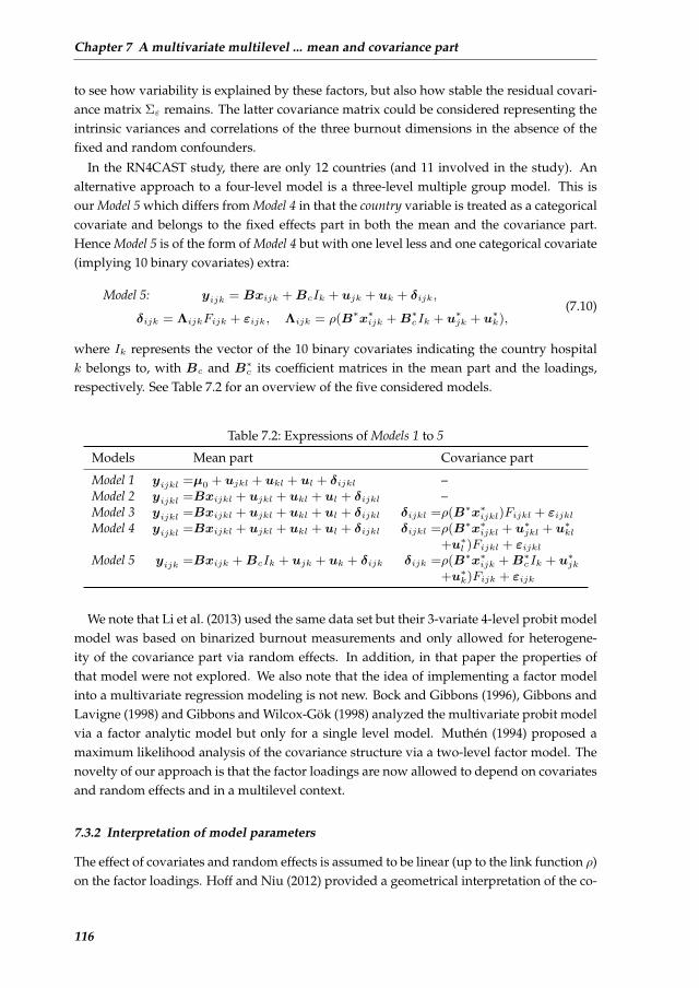
Chapter 7 A multivariate multilevel ... mean and covariance part
to see how variability is explained by these factors, but also how stable the residual covari-ance matrix Σε remains. The latter covariance matrix could be considered representing theintrinsic variances and correlations of the three burnout dimensions in the absence of thefixed and random confounders.
In the RN4CAST study, there are only 12 countries (and 11 involved in the study). Analternative approach to a four-level model is a three-level multiple group model. This isour Model 5 which differs from Model 4 in that the country variable is treated as a categoricalcovariate and belongs to the fixed effects part in both the mean and the covariance part.Hence Model 5 is of the form of Model 4 but with one level less and one categorical covariate(implying 10 binary covariates) extra:
Model 5: yijk = Bxijk +BcIk + ujk + uk + δijk,
δijk = ΛijkFijk + εijk, Λijk = ρ(B∗x∗ijk +B∗cIk + u∗jk + u∗k),(7.10)
where Ik represents the vector of the 10 binary covariates indicating the country hospitalk belongs to, with Bc and B∗c its coefficient matrices in the mean part and the loadings,respectively. See Table 7.2 for an overview of the five considered models.
Table 7.2: Expressions of Models 1 to 5
Models Mean part Covariance part
Model 1 yijkl =µ0 + ujkl + ukl + ul + δijkl –Model 2 yijkl =Bxijkl + ujkl + ukl + ul + δijkl –Model 3 yijkl =Bxijkl + ujkl + ukl + ul + δijkl δijkl =ρ(B∗x∗ijkl)Fijkl + εijklModel 4 yijkl =Bxijkl + ujkl + ukl + ul + δijkl δijkl =ρ(B∗x∗ijkl + u∗jkl + u∗kl
+u∗l )Fijkl + εijklModel 5 yijk =Bxijk +BcIk + ujk + uk + δijk δijk =ρ(B∗x∗ijk +B∗cIk + u∗jk
+u∗k)Fijk + εijk
We note that Li et al. (2013) used the same data set but their 3-variate 4-level probit modelmodel was based on binarized burnout measurements and only allowed for heterogene-ity of the covariance part via random effects. In addition, in that paper the properties ofthat model were not explored. We also note that the idea of implementing a factor modelinto a multivariate regression modeling is not new. Bock and Gibbons (1996), Gibbons andLavigne (1998) and Gibbons and Wilcox-Gok (1998) analyzed the multivariate probit modelvia a factor analytic model but only for a single level model. Muthen (1994) proposed amaximum likelihood analysis of the covariance structure via a two-level factor model. Thenovelty of our approach is that the factor loadings are now allowed to depend on covariatesand random effects and in a multilevel context.
7.3.2 Interpretation of model parameters
The effect of covariates and random effects is assumed to be linear (up to the link function ρ)on the factor loadings. Hoff and Niu (2012) provided a geometrical interpretation of the co-
116
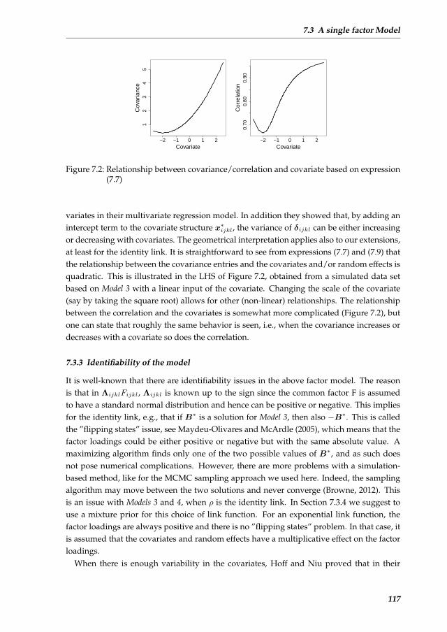
7.3 A single factor Model
−2 −1 0 1 21
23
45
Covariate
Cov
aria
nce
−2 −1 0 1 2
0.70
0.80
0.90
Covariate
Cor
rela
tion
Figure 7.2: Relationship between covariance/correlation and covariate based on expression(7.7)
variates in their multivariate regression model. In addition they showed that, by adding anintercept term to the covariate structure x∗ijkl, the variance of δijkl can be either increasingor decreasing with covariates. The geometrical interpretation applies also to our extensions,at least for the identity link. It is straightforward to see from expressions (7.7) and (7.9) thatthe relationship between the covariance entries and the covariates and/or random effects isquadratic. This is illustrated in the LHS of Figure 7.2, obtained from a simulated data setbased on Model 3 with a linear input of the covariate. Changing the scale of the covariate(say by taking the square root) allows for other (non-linear) relationships. The relationshipbetween the correlation and the covariates is somewhat more complicated (Figure 7.2), butone can state that roughly the same behavior is seen, i.e., when the covariance increases ordecreases with a covariate so does the correlation.
7.3.3 Identifiability of the model
It is well-known that there are identifiability issues in the above factor model. The reasonis that in ΛijklFijkl, Λijkl is known up to the sign since the common factor F is assumedto have a standard normal distribution and hence can be positive or negative. This impliesfor the identity link, e.g., that if B∗ is a solution for Model 3, then also −B∗. This is calledthe ”flipping states” issue, see Maydeu-Olivares and McArdle (2005), which means that thefactor loadings could be either positive or negative but with the same absolute value. Amaximizing algorithm finds only one of the two possible values of B∗, and as such doesnot pose numerical complications. However, there are more problems with a simulation-based method, like for the MCMC sampling approach we used here. Indeed, the samplingalgorithm may move between the two solutions and never converge (Browne, 2012). Thisis an issue with Models 3 and 4, when ρ is the identity link. In Section 7.3.4 we suggest touse a mixture prior for this choice of link function. For an exponential link function, thefactor loadings are always positive and there is no ”flipping states” problem. In that case, itis assumed that the covariates and random effects have a multiplicative effect on the factorloadings.
When there is enough variability in the covariates, Hoff and Niu proved that in their
117

Chapter 7 A multivariate multilevel ... mean and covariance part
model all parameters are identifiable up to a sign. For Model 3, we sketch in Appendix 7.9that this result must also hold. For Model 4, things are more complex. To prove likelihoodidentifiability in mixed models is generally complex, as indicated in Wu (2010). In addition,the random effects for Model 4 are only determined up to the sign, which can be seen fromthe trace plots. Post-processing of the Markov chain of each random effect in the covariancepart was therefore necessary to obtain its posterior mean (up to the sign), for this we usedthe R function normalmixEM from the mixtools package. Then a QQ-plot based on a foldednormal distribution was used to assess the normality assumption (up to the sign) of theserandom effects. More details can be found in the Supplementary Material 1.
7.3.4 Priors
We have opted for a Bayesian approach to estimate the model parameters, which requires aprior distribution for all its parameters. One of the benefits of applying a Bayesian approachis that prior information can be incorporated into the analysis, if available. Two problemswere encountered to include prior information into the model. The first problem relates tothe way we deal with the bounded outcome score response (more details in Section 7.7). Theparameter estimates from this approach are difficult to compare with those obtained from alogistic model (using binary or categorical responses) or from a linear model using the origi-nal burnout scores. Secondly, it is hard to imagine what should constitute reasonable valuesof the parameters in the factor analytic model of the covariance structure. However, becauseof the huge sample size of our study, practically each prior information on the parametershas a negligible effect on the posterior estimates. That is why we finally chose a vague nor-mal prior (with mean zero and variance 106) for regression parameters (B-parameters) anda vague inverse Wishart prior (with small diagonal values, say 0.01, for the scale matrix anddegrees of freedom equal to the dimension of the matrix (Lesaffre and Lawson, 2012)) forthe covariance matrices of the random effects in the mean and the loadings, i.e. Σv and Σ∗v
(with v = u, h, c). Note that constraining the off-diagonal elements to zero may speed upthe convergence of the chain considerably.
It is, however, more difficult to specify the prior distribution for theB∗-parameters in thefactor loadings because of the ”flipping states” identifiability problem mentioned in Section7.3.3. This identification problem needs to be taken into account when sampling the randomeffects in the factor loadings. In Appendix 7.9 we show the JAGS (Just Another Gibbs Sam-pler) program (based on the R package rjags (Plummer, 2013)) for a simple version of Model4, i.e. yij = µ+uj+(β∗0 +β∗1x
∗ij+u∗j )Fij+εij . For Lj = β∗0 +u∗j , we have taken the mixture
prior 0.5N(−µ∗0,Σ∗u)+0.5N(µ∗0,Σ∗u) withµ∗0 given a classical (vague) independent normal
prior. Half of the Lj will fluctuate around µ∗0 while the other half around −µ∗0. The slopesβ∗1 and −β∗1 will also be sampled from a mixture, but the sign will be determined from thesign of β∗0 when the covariates show enough variation as can be deduced from Section 7.3.3and Appendix 7.9. Note that the MCMC procedure with the mixture prior for the factorloading parameters is needed when the identity link is used, but not for the exponential
1All Supplementary materials in this chapter can be found in the website:http://onlinelibrary.wiley.com/doi/10.1002/sim.6062/suppinfo.
118
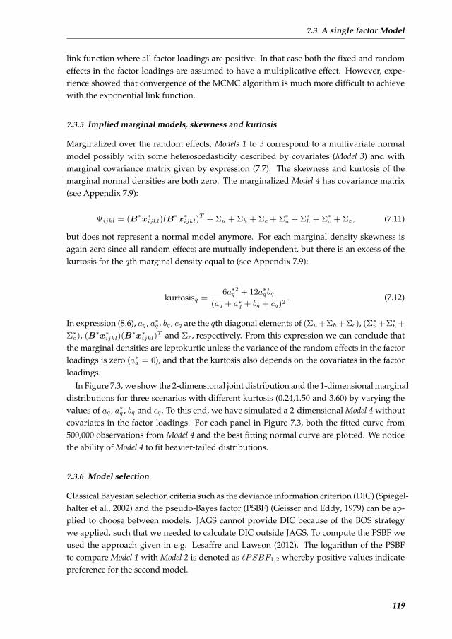
7.3 A single factor Model
link function where all factor loadings are positive. In that case both the fixed and randomeffects in the factor loadings are assumed to have a multiplicative effect. However, expe-rience showed that convergence of the MCMC algorithm is much more difficult to achievewith the exponential link function.
7.3.5 Implied marginal models, skewness and kurtosis
Marginalized over the random effects, Models 1 to 3 correspond to a multivariate normalmodel possibly with some heteroscedasticity described by covariates (Model 3) and withmarginal covariance matrix given by expression (7.7). The skewness and kurtosis of themarginal normal densities are both zero. The marginalized Model 4 has covariance matrix(see Appendix 7.9):
Ψijkl = (B∗x∗ijkl)(B∗x∗ijkl)
T + Σu + Σh + Σc + Σ∗u + Σ∗h + Σ∗c + Σε, (7.11)
but does not represent a normal model anymore. For each marginal density skewness isagain zero since all random effects are mutually independent, but there is an excess of thekurtosis for the qth marginal density equal to (see Appendix 7.9):
kurtosisq =6a∗2q + 12a∗qbq
(aq + a∗q + bq + cq)2. (7.12)
In expression (8.6), aq , a∗q , bq , cq are the qth diagonal elements of (Σu+Σh+Σc), (Σ∗u+Σ∗h+
Σ∗c), (B∗x∗ijkl)(B∗x∗ijkl)
T and Σε, respectively. From this expression we can conclude thatthe marginal densities are leptokurtic unless the variance of the random effects in the factorloadings is zero (a∗q = 0), and that the kurtosis also depends on the covariates in the factorloadings.
In Figure 7.3, we show the 2-dimensional joint distribution and the 1-dimensional marginaldistributions for three scenarios with different kurtosis (0.24,1.50 and 3.60) by varying thevalues of aq , a∗q , bq and cq . To this end, we have simulated a 2-dimensional Model 4 withoutcovariates in the factor loadings. For each panel in Figure 7.3, both the fitted curve from500,000 observations from Model 4 and the best fitting normal curve are plotted. We noticethe ability of Model 4 to fit heavier-tailed distributions.
7.3.6 Model selection
Classical Bayesian selection criteria such as the deviance information criterion (DIC) (Spiegel-halter et al., 2002) and the pseudo-Bayes factor (PSBF) (Geisser and Eddy, 1979) can be ap-plied to choose between models. JAGS cannot provide DIC because of the BOS strategywe applied, such that we needed to calculate DIC outside JAGS. To compute the PSBF weused the approach given in e.g. Lesaffre and Lawson (2012). The logarithm of the PSBFto compare Model 1 with Model 2 is denoted as `PSBF1,2 whereby positive values indicatepreference for the second model.
119
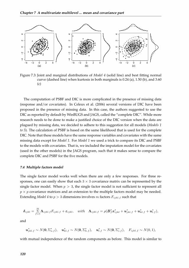
Chapter 7 A multivariate multilevel ... mean and covariance part
●
●
●
●
●
●●
●
●
●
●
●
●
●
●
●
●●
●
●
●
●
●
●
●
●
●
●
●
●
●
●
●
●
●
●
●
●
●
●●
●
●
●
●
●
●
●
●
●
●
●
●
●
●
●
●
● ●
●
●
●
●
●
●
●●
●
●
●
●
●
●
●
●
●
●
●
●
●
●
●
●
●
●
●
●
●
●
●
●
●
●
●
● ●
●
●
●
●
−4 −2 0 2 4
−4
−2
02
4
(a)
●
●
●
●
●●
●
●
●
●
●
●
●
●
●
●
●
●
●
●
●
●
●
●
●
●
●
●
●
●
●
●
●
●
●
●
●
●
●
●
●
●
●
●
●
●●
●
●
●
●
●
●
●
●
●
●
●
●
●
●
●
●
●
●
●
●
●
●
●
●
●●
●
●
●
●
●
●
●
●
●
●
●
●
●
●
●
●
●
●
●
●
●
●
●
●
●
●
●
−4 −2 0 2 4
−4
−2
02
4(b)
●
●
●
●
●
●
●
●
●
●
● ●
●
●
●
●
●
●
●
●
●
●
●
●
●
●
●
●
●
●
●
●
●
●
●
●
●
●
●
●
●
●
●
●
●
●
●
●
●
●
●
●
●●
● ●
●
●
●
●
●
● ●
●
●
●
●
●
●
●
●
●
● ●
●
●
● ●
●●
●
●
●
● ●
●
●
●
●
●
●
●
●●●
●
●
●
●
●
−4 −2 0 2 4
−4
−2
02
4
(c)
Figure 7.3: Joint and marginal distributions of Model 4 (solid line) and best fitting normalcurve (dashed line) when kurtosis in both marginals is 0.24 (a), 1.50 (b), and 3.60(c)
The computation of PSBF and DIC is more complicated in the presence of missing data(response and/or covariates). In Celeux et al. (2006) several versions of DIC have beenproposed in the presence of missing data. In this case, the authors suggested to use theDIC as reported by default by WinBUGS and JAGS, called the “complete DIC”. While moreresearch needs to be done to make a justified choice of the DIC version when the data areplagued by missing data, we decided to adhere to this suggestion for all models (Models 1to 5). The calculation of PSBF is based on the same likelihood that is used for the completeDIC. Note that these models have the same response variables and covariates with the samemissing data except for Model 1. For Model 1 we used a trick to compare its DIC and PSBFto the models with covariates. That is, we included the imputation model for the covariates(used in the other models) in the JAGS program, such that it makes sense to compare thecomplete DIC and PSBF for the five models.
7.4 Multiple factors model
The single factor model works well when there are only a few responses. For three re-sponses, one can easily show that each 3 × 3 covariance matrix can be represented by thesingle factor model. When p > 3, the single factor model is not sufficient to represent allp × p covariance matrices and an extension to the multiple factors model may be needed.Extending Model 4 to p > 3 dimensions involves m factors Fijkl.f such that
δijkl =m
Σf=1
Λijkl.fFijkl.f + εijkl, with Λijkl.f = ρ(B∗fx∗ijkl + u∗jkl.f + u∗kl.f + u∗l.f ),
and
u∗jkl.f ∼ N(0,Σ∗u.f ), u∗kl.f ∼ N(0,Σ∗h.f ), u∗l.f ∼ N(0,Σ∗c.f ), Fijkl.f ∼ N(0, 1),
with mutual independence of the random components as before. This model is similar to
120
7.5 Computational procedure
Hoff and Niu’s rank −m model but now in a multilevel context.
As for Hoff and Niu’s rank − m model, the intercept matrix B∗0 in the factor loadings,which has p × m elements with p the dimension of the outcome, should have orthogonalcolumns. Besides, same as in Model 4, the mixture prior for the factor loadings should beapplied for each factor. In addition, the identifiability issues are similar to those of Model 4but more involved. This is a topic of future research.
Fox and Dunson (2011) pointed out that with Hoff and Niu’s rank −m model the totalnumber of parameters dramatically increase with increasing m when the dimensionality ofthe outcome is high. They suggested an alternative approach, which could be adopted alsohere. Reducing the high dimensionality of the outcome is, however, not the focus in thispaper as this model is not needed for our motivating data set.
7.5 Computational procedure
A JAGS program of each model was written for the analysis of the motivating data set.Models 1 and 2 were estimated with the R package rjags, while the dclone package was usedfor the other models, which is based on JAGS with multiple cores. The DIC calculation wasbased on the dic.samples() function, which corrects for overoptimism in computing theclassical DIC (Plummer, 2002). PSBF was calculated following the way described in Lesaffreand Lawson (2012). A 2-level version of the program for Model 4 can be found in Appendix7.9. The 4-level program can be derived from this program but is available from the firstauthor upon request.
Three chains were initialized with different starting values for all models. For Models 1and 2, 10,000 iterations were conducted with the first half as the burn-in part, while forModels 3 to 5 100,000 iterations were set with the first 70,000 as burn-in part. Convergencewas decided when the Brooks-Gelman-Rubin plots showed good behavior indicated by theestimate Rhat < 1.1 (Brooks and Gelman, 1998). In addition, the Monte Carlo error of theposterior mean should be around or less than 5% of the posterior SD. Upon convergence,we computed the posterior median for the variance components and the posterior mean forthe remaining parameters together with the equal tail 95% credible interval (CI). Both DICand `PSBF were used to select the most appropriate model.
7.6 Missing data
The RN4CAST project is plagued with a relatively large non-response rate, but also withmissingness in the response and the covariates. Therefore, consideration is needed on theeffect of missing information on the substantive conclusions of the analysis, but also onwhat can be done to reduce possible bias due to lacking data. Below we consider the threeproblems separately, suggest solutions if possible and/or reflect on what might the possibleimpact of the non-response/missingness. Although trivial, we note that our suggested mul-tivariate multilevel model remains valid whether or not the study is plagued with missingdata.
121
Chapter 7 A multivariate multilevel ... mean and covariance part
7.6.1 Non-response
In Section 7.2.1 we described that there is considerable non-response in the RN4CAST studyespecially at hospital and nurse level. Around six out of ten (63.55%) hospitals that wereinvited to this study agreed to participate. At the planning stage of the study, representa-tive checks (hospital type, size) were carried out in each country to assure that the samplerepresents the population appropriately. When necessary, corrective actions (such as extramotivating hospitals to participate) were taken to improve representativeness of the par-ticipating hospitals. The response rates of the nurses were around 40% in the differentcountries. Thus, at best we can claim that all reasonable efforts (this was a huge study) wereundertaken to improve the representativeness of the study, but bias due to non-responsecannot be excluded. One referee suggests to implement a corrective action in estimatingthe model parameters making use of the approach described in e.g. Kott (1994). However,this kind of correction needs covariate information of all subjects, which was not availablein the RN4CAST study for the non-responders. We note that in a similar survey amongUS nurses (Smith, 2008) the author assessed the non-response bias. More particularly, theauthor randomly sampled non-respondents and was able to motivate them to fill in (at thevery end) the questionnaires. He found indeed some differences in the non-responders’demographic characteristics compared to the initial responders. However, no differenceswere found with regard to nurses’ assessments of their work environment and burnout.This supported our hope and belief that chances are low that our findings are dramaticallyaffected by systematic tendencies of certain respondents to have opted into our survey or tohave opted out.
7.6.2 Missingness in the burnout measurements
The three burnout outcomes are sum scores of the items within each dimension respectively.Around 10% of the nurses have at least one of the 22 items missing. This implies that forthese subjects some or all burnout scores were too low. Imputation of the missing item wasdone by treating the scores with missing items as interval censored data with the currentvalue as the lower limit of the interval (equivalent to assigning zeros to the missing items)and the upper limit of the interval obtained by taking the largest value for each missingitem, which is 6 in this case. It can easily be seen that the interval censored trick combineswell with the BOS approach we utilized across the whole analysis.
7.6.3 Missing covariates
Missingness also plagued the covariates, but primarily working experience with about 6.3%of the subjects not filled in this item. A classical approach to deal with missing covariates isto make use of multiple imputation. This is a fairly straightforward approach with MCMCsoftware. Indeed, it only involves to sample at each iteration, in parallel to the main esti-mation program, the missing covariate values using an appropriate imputation model andplug-in the sampled value into the main model. The chosen model for imputation is a Gaus-sian linear regression model including all the other covariates in Table 8.1 as predictors. See
122

7.7 Analysis of the RN4CAST burnout data
the Supplementary Material for the actual models chosen to estimate the missing covariatevalues.
7.7 Analysis of the RN4CAST burnout data
7.7.1 Choice of response and covariates
Figure 7.1 shows a skewed distribution for each of the three burnout measurements. Be-cause the measurements are in fact discrete with a non-trivial portion of zeros they cannot betransformed to normality with common transformations. However, since the burnout mea-surements are examples of a bounded outcome score (BOS), one may apply the techniquesuggested by Lesaffre et al. (2007). This technique assumes that a standardized version ofthe burnout measurement is a coarsened latent continuous variable which has a Gaussiandistribution after a logit transformation. More specifically, the observed response is firsttransformed to a (discrete) response y on the unit interval (by a change of scale). Then a la-tent random variable z on (0,1) is assumed, with the property that log[z/(1− z)] ∼ N(µ, σ2)
and such that y is obtained by coarsening z. In our analysis, we applied this techniqueon each of the three burnout measurements. Models 1 to 5 were then defined on the latentcontinuous outcomes.
The candidate covariates involved in the mean and/or variance structures in later anal-yses, are listed in Table 8.1. In order to make the regression coefficients of these variablescomparable and to improve computational properties, standardized covariates (mean=0,SD=1) were used in later analyses. In addition, in order to investigate the level-specific ef-fects of the covariates the following decomposition was made, as suggested by Neuhausand Kalbfleisch (1998):
xijkl = (xijkl − xjkl) + (xjkl − xkl) + (xkl − xl) + xl
= xn + xu + xh + xc,(7.13)
xjkl = 1njkl
∑njkl
i=1 xijkl and similarly for the other means. In expression (8.7), the lowestlevel variable is partitioned into four parts corresponding to the four levels, i.e. n for nurse,u for nursing unit, h for hospital and c for country. By doing so, we study the ”pure” effectof the covariates at each level (for work environment, there is no nurse-level partition becausethe lowest level measurement is nursing unit).
We now address the three research questions mentioned in Section 7.2. For each modelfitted to the data, we describe the variability of the means of the burnout measurements atthe different levels separately from the variability (and correlation) of these measurementsat the nurse level. The parameter estimates for all five models can be found in the Supple-mentary Material of the paper.
123
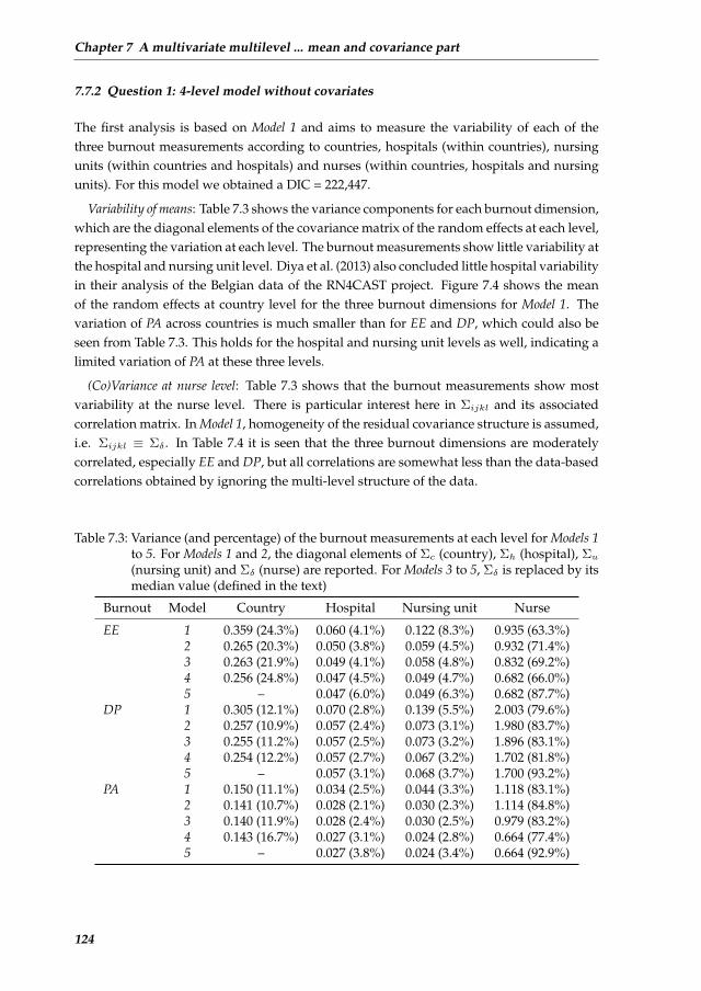
Chapter 7 A multivariate multilevel ... mean and covariance part
7.7.2 Question 1: 4-level model without covariates
The first analysis is based on Model 1 and aims to measure the variability of each of thethree burnout measurements according to countries, hospitals (within countries), nursingunits (within countries and hospitals) and nurses (within countries, hospitals and nursingunits). For this model we obtained a DIC = 222,447.
Variability of means: Table 7.3 shows the variance components for each burnout dimension,which are the diagonal elements of the covariance matrix of the random effects at each level,representing the variation at each level. The burnout measurements show little variability atthe hospital and nursing unit level. Diya et al. (2013) also concluded little hospital variabilityin their analysis of the Belgian data of the RN4CAST project. Figure 7.4 shows the meanof the random effects at country level for the three burnout dimensions for Model 1. Thevariation of PA across countries is much smaller than for EE and DP, which could also beseen from Table 7.3. This holds for the hospital and nursing unit levels as well, indicating alimited variation of PA at these three levels.
(Co)Variance at nurse level: Table 7.3 shows that the burnout measurements show mostvariability at the nurse level. There is particular interest here in Σijkl and its associatedcorrelation matrix. In Model 1, homogeneity of the residual covariance structure is assumed,i.e. Σijkl ≡ Σδ . In Table 7.4 it is seen that the three burnout dimensions are moderatelycorrelated, especially EE and DP, but all correlations are somewhat less than the data-basedcorrelations obtained by ignoring the multi-level structure of the data.
Table 7.3: Variance (and percentage) of the burnout measurements at each level for Models 1to 5. For Models 1 and 2, the diagonal elements of Σc (country), Σh (hospital), Σu(nursing unit) and Σδ (nurse) are reported. For Models 3 to 5, Σδ is replaced by itsmedian value (defined in the text)
Burnout Model Country Hospital Nursing unit Nurse
EE 1 0.359 (24.3%) 0.060 (4.1%) 0.122 (8.3%) 0.935 (63.3%)2 0.265 (20.3%) 0.050 (3.8%) 0.059 (4.5%) 0.932 (71.4%)3 0.263 (21.9%) 0.049 (4.1%) 0.058 (4.8%) 0.832 (69.2%)4 0.256 (24.8%) 0.047 (4.5%) 0.049 (4.7%) 0.682 (66.0%)5 – 0.047 (6.0%) 0.049 (6.3%) 0.682 (87.7%)
DP 1 0.305 (12.1%) 0.070 (2.8%) 0.139 (5.5%) 2.003 (79.6%)2 0.257 (10.9%) 0.057 (2.4%) 0.073 (3.1%) 1.980 (83.7%)3 0.255 (11.2%) 0.057 (2.5%) 0.073 (3.2%) 1.896 (83.1%)4 0.254 (12.2%) 0.057 (2.7%) 0.067 (3.2%) 1.702 (81.8%)5 – 0.057 (3.1%) 0.068 (3.7%) 1.700 (93.2%)
PA 1 0.150 (11.1%) 0.034 (2.5%) 0.044 (3.3%) 1.118 (83.1%)2 0.141 (10.7%) 0.028 (2.1%) 0.030 (2.3%) 1.114 (84.8%)3 0.140 (11.9%) 0.028 (2.4%) 0.030 (2.5%) 0.979 (83.2%)4 0.143 (16.7%) 0.027 (3.1%) 0.024 (2.8%) 0.664 (77.4%)5 – 0.027 (3.8%) 0.024 (3.4%) 0.664 (92.9%)
124
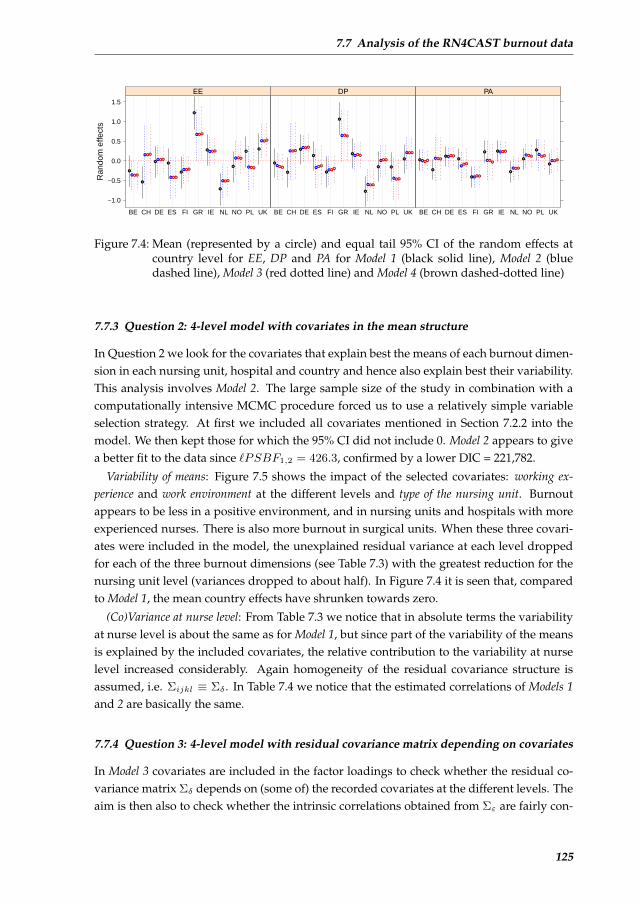
7.7 Analysis of the RN4CAST burnout data
Ran
dom
effe
cts
−1.0
−0.5
0.0
0.5
1.0
1.5
BE CH DE ES FI GR IE NL NO PL UK
●
●
●
●
●
●
●
●
●
●
●
●
●
●
●
●
●
●
●
●
●
●
●
●
●
●
●
●
●
●
●
●
●
●
●
●
●
●
●
●
●
●
●
●
EE
BE CH DE ES FI GR IE NL NO PL UK
●
●
●
●
●
●
● ●
●
●
●
●
●
●
●
●
●
●
●
●
●
●
●
●
●
●
●
●
●
●
●
●
●
●
●
●
●
●
●
●
●
●
●
●
DP
BE CH DE ES FI GR IE NL NO PL UK
●
●
●
●
● ●
●
●
●
●●
● ●
●
●
●
●● ●
●
●
●
● ●
●
●
●
●
● ●
●
●
●
● ●
●
●
●
●
● ●
●
●
●
PA
Figure 7.4: Mean (represented by a circle) and equal tail 95% CI of the random effects atcountry level for EE, DP and PA for Model 1 (black solid line), Model 2 (bluedashed line), Model 3 (red dotted line) and Model 4 (brown dashed-dotted line)
7.7.3 Question 2: 4-level model with covariates in the mean structure
In Question 2 we look for the covariates that explain best the means of each burnout dimen-sion in each nursing unit, hospital and country and hence also explain best their variability.This analysis involves Model 2. The large sample size of the study in combination with acomputationally intensive MCMC procedure forced us to use a relatively simple variableselection strategy. At first we included all covariates mentioned in Section 7.2.2 into themodel. We then kept those for which the 95% CI did not include 0. Model 2 appears to givea better fit to the data since `PSBF1,2 = 426.3, confirmed by a lower DIC = 221,782.
Variability of means: Figure 7.5 shows the impact of the selected covariates: working ex-perience and work environment at the different levels and type of the nursing unit. Burnoutappears to be less in a positive environment, and in nursing units and hospitals with moreexperienced nurses. There is also more burnout in surgical units. When these three covari-ates were included in the model, the unexplained residual variance at each level droppedfor each of the three burnout dimensions (see Table 7.3) with the greatest reduction for thenursing unit level (variances dropped to about half). In Figure 7.4 it is seen that, comparedto Model 1, the mean country effects have shrunken towards zero.
(Co)Variance at nurse level: From Table 7.3 we notice that in absolute terms the variabilityat nurse level is about the same as for Model 1, but since part of the variability of the meansis explained by the included covariates, the relative contribution to the variability at nurselevel increased considerably. Again homogeneity of the residual covariance structure isassumed, i.e. Σijkl ≡ Σδ . In Table 7.4 we notice that the estimated correlations of Models 1and 2 are basically the same.
7.7.4 Question 3: 4-level model with residual covariance matrix depending on covariates
In Model 3 covariates are included in the factor loadings to check whether the residual co-variance matrix Σδ depends on (some of) the recorded covariates at the different levels. Theaim is then also to check whether the intrinsic correlations obtained from Σε are fairly con-
125
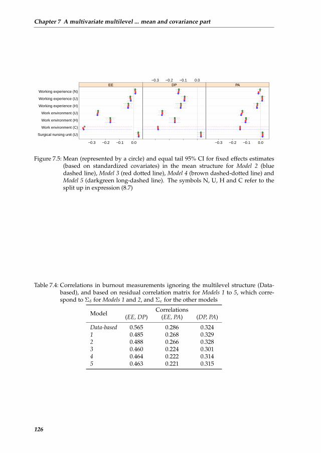
Chapter 7 A multivariate multilevel ... mean and covariance part
Surgical nursing unit (U)
Work environment (C)
Work environment (H)
Work environment (U)
Working experience (H)
Working experience (U)
Working experience (N)
−0.3 −0.2 −0.1 0.0
●
●
●
●
●
●
●
●
●
●
●
●
●
●
●
●
●
●
●
●
●
●
●
●
●
●
●
EE−0.3 −0.2 −0.1 0.0
●
●
●
●
●
●
●
●
●
●
●
●
●
●
●
●
●
●
●
●
●
●
●
●
●
●
●
DP
−0.3 −0.2 −0.1 0.0
●
●
●
●
●
●
●
●
●
●
●
●
●
●
●
●
●
●
●
●
●
●
●
●
●
●
●
PA
Figure 7.5: Mean (represented by a circle) and equal tail 95% CI for fixed effects estimates(based on standardized covariates) in the mean structure for Model 2 (bluedashed line), Model 3 (red dotted line), Model 4 (brown dashed-dotted line) andModel 5 (darkgreen long-dashed line). The symbols N, U, H and C refer to thesplit up in expression (8.7)
Table 7.4: Correlations in burnout measurements ignoring the multilevel structure (Data-based), and based on residual correlation matrix for Models 1 to 5, which corre-spond to Σδ for Models 1 and 2, and Σε for the other models
Model Correlations(EE, DP) (EE, PA) (DP, PA)
Data-based 0.565 0.286 0.3241 0.485 0.268 0.3292 0.488 0.266 0.3283 0.460 0.224 0.3014 0.464 0.222 0.3145 0.463 0.221 0.315
126
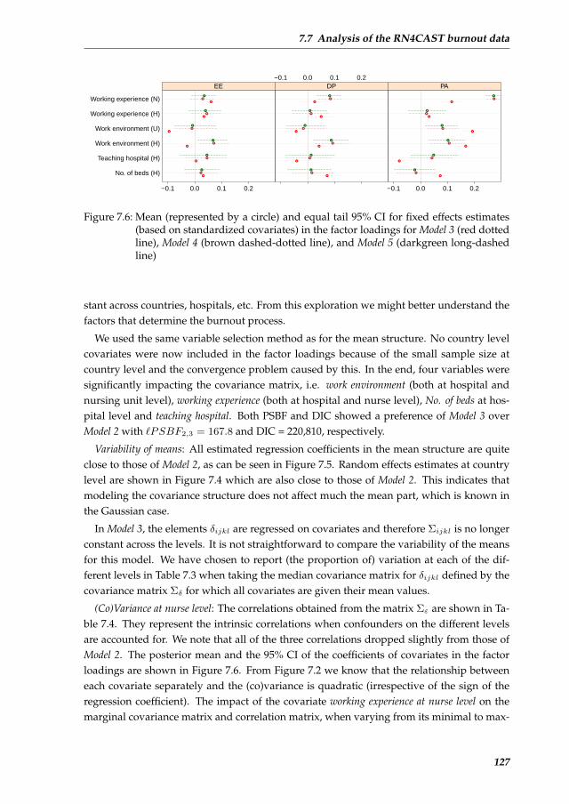
7.7 Analysis of the RN4CAST burnout data
No. of beds (H)
Teaching hospital (H)
Work environment (H)
Work environment (U)
Working experience (H)
Working experience (N)
−0.1 0.0 0.1 0.2
●
●
●
●
●
●
●
●
●
●
●
●
●
●
●
●
●
●
EE−0.1 0.0 0.1 0.2
●
●
●
●
●
●
●
●
●
●
●
●
●
●
●
●
●
●
DP
−0.1 0.0 0.1 0.2
●
●
●
●
●
●
●
●
●
●
●
●
●
●
●
●
●
●
PA
Figure 7.6: Mean (represented by a circle) and equal tail 95% CI for fixed effects estimates(based on standardized covariates) in the factor loadings for Model 3 (red dottedline), Model 4 (brown dashed-dotted line), and Model 5 (darkgreen long-dashedline)
stant across countries, hospitals, etc. From this exploration we might better understand thefactors that determine the burnout process.
We used the same variable selection method as for the mean structure. No country levelcovariates were now included in the factor loadings because of the small sample size atcountry level and the convergence problem caused by this. In the end, four variables weresignificantly impacting the covariance matrix, i.e. work environment (both at hospital andnursing unit level), working experience (both at hospital and nurse level), No. of beds at hos-pital level and teaching hospital. Both PSBF and DIC showed a preference of Model 3 overModel 2 with `PSBF2,3 = 167.8 and DIC = 220,810, respectively.
Variability of means: All estimated regression coefficients in the mean structure are quiteclose to those of Model 2, as can be seen in Figure 7.5. Random effects estimates at countrylevel are shown in Figure 7.4 which are also close to those of Model 2. This indicates thatmodeling the covariance structure does not affect much the mean part, which is known inthe Gaussian case.
In Model 3, the elements δijkl are regressed on covariates and therefore Σijkl is no longerconstant across the levels. It is not straightforward to compare the variability of the meansfor this model. We have chosen to report (the proportion of) variation at each of the dif-ferent levels in Table 7.3 when taking the median covariance matrix for δijkl defined by thecovariance matrix Σδ for which all covariates are given their mean values.
(Co)Variance at nurse level: The correlations obtained from the matrix Σε are shown in Ta-ble 7.4. They represent the intrinsic correlations when confounders on the different levelsare accounted for. We note that all of the three correlations dropped slightly from those ofModel 2. The posterior mean and the 95% CI of the coefficients of covariates in the factorloadings are shown in Figure 7.6. From Figure 7.2 we know that the relationship betweeneach covariate separately and the (co)variance is quadratic (irrespective of the sign of theregression coefficient). The impact of the covariate working experience at nurse level on themarginal covariance matrix and correlation matrix, when varying from its minimal to max-
127

Chapter 7 A multivariate multilevel ... mean and covariance part
Working experience
Var
ianc
e E
E
−24.82 4.34 33.5
0.85
0.94
1.11
Working experience
Cov
aria
nce
EE
& D
P
−24.82 4.34 33.5
0.6
0.67
0.77
Working experience
Cov
aria
nce
EE
& P
A
−24.82 4.34 33.5
0.19
0.3
0.57
Working experience
corr
elat
ion
EE
& D
P
−24.82 4.34 33.5
0.47
0.49
0.51
Working experience
Var
ianc
e D
P
−24.82 4.34 33.5
1.93
1.97
2.03
Working experience
Cov
aria
nce
DP
& P
A
−24.82 4.34 33.5
0.4
0.5
0.67
Working experience
Cor
rela
tion
EE
& P
A
−24.82 4.34 33.5
0.21
0.3
0.45
Working experience
Cor
rela
tion
DP
& P
A
−24.82 4.34 33.5
0.29
0.34
0.39
Working experience
Var
ianc
e PA
−24.82 4.34 33.5
0.98
1.08
1.47
Figure 7.7: Dependence of covariance matrix Σijkl in equation (7.7) (upper trian-gle)/associated correlation matrix and working experience at nurse level. The max-imum, minimum and the median values of the covariate are marked
imal value, is shown in Figure 7.7. Especially the correlations with PA seem to dependhighly on working experience at nurse level, implying that the longer the professional career ofthe nurse the more emotional exhaustion and depersonalization the less self-esteemed thenurse is. When varying B
∗fx∗ijkl from its minimal to its maximal value, e.g. the correlation
between EE and PA now ranges from -0.25 to 0.55 and the variance of PA ranges from 0.97to 2.52.
7.7.5 Question 3: 4-level model with residual covariance matrix depending oncovariates and random effects
Finally, we included random effects into the covariance structure to accommodate for themeasurement error in the included covariates in the factor loadings, for not-included (andpossibly not measured) important covariates and to protect against potential outlying en-tries. This analysis involves Model 4. With `PSBF3,4 = 1255.7 there is a strong indicationthat Model 4 fits the data better than Model 3. This is confirmed by a much lower DIC =213,908.
Variability of means: From Figure 7.5 we see that the fixed effects estimates are basicallythe same as those of Models 2 and 3, which is also the case for the random effects at countrylevel (Figure 7.4). The entries in Table 7.3 for Model 4 again correspond to the median valuedetermined in Σδ , i.e. by taking the mean value for each covariate, as well as zero for therandom effects in the factor loadings.
(Co)Variance at nurse level: We see from Table 7.4 that there is remarkable stability of thecorrelations between Model 4 and the previous model. From Figure 7.6 we note that, addingrandom effects in the factor loadings, renders three hospital-level covariates non-significant,
128
7.7 Analysis of the RN4CAST burnout data
i.e. working experience, teaching hospital and No. of beds. In general, we observe that both theestimates as well as the 95% CI are reasonably affected by including the random effects.The interpretation of this result is not straightforward, but definitely the included randomeffects appear to be associated with these three covariates. Judging from the DIC and PSBFModel 4 seems to be preferable, which could imply that ignoring random effects in the factorloadings results in biasedly estimated regression coefficients (and SEs) in the factor loadings.We also plotted the mean random effects at the country level in the factor loadings (notshown), again Greece showed some outlying behavior but to a lesser extent.
7.7.6 A multiple group 3-level model with residual covariance matrix depending oncovariates and random effects
As there are only 11 countries, an alternative is to run a 3-level multiple group model (Model5), treating the 11 countries as fixed effects both in the mean structure and the factor load-ing structure. Except for this change all other settings are exactly the same as for Model 4.Belgium was taken as reference country. With `PSBF4,5 = 82.1 and DIC = 213,885, Model5 is preferred to Model 4. However, the changes in PSBF and DIC are relatively small, es-pecially for DIC that dropped only 23. Considering the large sample size, the difference inperformance between the two models is not great.
Variability of means: The variances partitioned at each level are listed in Table 7.3, againthe median estimates are shown. Note that as country was treated as a fixed effect, weactually took the median values for the reference country, i.e. Belgium. Figure 7.5 showsthat the fixed effects (except for the country effects) estimates in the mean structure are quiteclose to those from other models. For the country fixed effects (not shown), we noticed thatSwitzerland, the Netherlands and Finland score better on burnout than the reference countryBelgium, while Spain, Poland, Ireland, Greece and Germany score worse.
(Co)Variance at nurse level: The parameter estimates in the factor loadings are quite close tothose in Model 4, see Figure 7.6. The intrinsic correlations between the burnout dimensionsare close to those of Model 3.
7.7.7 Model assessment
The assessment of Model 4 was performed in this section. More specifically, we did threekinds of assessments. Firstly, a posterior predictive check (PPC) based on Gelman’s chi-square statistic (Gelman et al., 2013) was performed to find evidence of the goodness-of-fitof the models for each of the burnout responses separately. Secondly, we conducted a nor-mality check for the random effects to justify the model assumption and further ran themodel with a multivariate t(3)- distribution for the random effects. Thirdly, the currentstrategy of handling missing data was compared with an alternative way, i.e. imputingthe missingness for the response variables prior to the analysis and removing the data withmissing covariate. Not only the parameter estimates of Model 4, but also the model selectionbased on DIC and PSBF were compared using the two strategies of handling missing data.More details for the second and third model assessments are described in the Supplemen-
129
Chapter 7 A multivariate multilevel ... mean and covariance part
tary Material. As a result, we found that the current model showed an acceptable fit to thedata, with PPC values for the three burnout dimensions being 0.36, 0.28 and 0.29, respec-tively. The normality assumption basically holds for all random effects in both the meanand the loadings as evidenced from the QQ-plots described in Section (7.3.3). Further, noqualitative changes were found in the model with multivariate t distribution. Finally, thetwo strategies of dealing with missing data for both the response and the covariate providedquite close estimates. Both DICs and `PSBFs are highly consistent with each other for thetwo strategies except for `PSBF2,3. Nevertheless, we believe that the current approach ofdealing with the missing information is preferable.
7.7.8 Some clinical conclusions
The primary clinical finding of this study is that all proposed models posit the importanceof nurses’ work environment, both at the hospital and nursing unit level, in explaining allthree dimensions of burnout. This pinpoints the key role that hospital health resourcesmanagement and front-line nurse leaders play in developing positive work environmentsto prevent burnout. Maslach and Leiter (2008) in their (2008) longitudinal study on burnoutchanges over a 1-year interval highlighted the importance of customized preventive inter-ventions. As proposed by these authors, such interventions should take place at an orga-nizational level, since burnout tends to cluster within particular groups. In dealing withburnout, hospitals and health care organizations in general should therefore continuouslyevaluate burnout and predicting features within the organizational climate.
The second finding is that the intrinsic correlations, as reported in Table 7.4 are relativelystable across the five models. But we could also notice that several factors determine thecovariance structure and hence will have an impact on the association structure of the threeburnout dimensions. We have illustrated this by showing that, as working experience in-creases, the correlation between EE and PA increases. This might corroborate the findingthat EE and PA develop in parallel within a problematic organizational environment with-out any major causal links between the two (Schaufeli et al., 1996).
7.8 Simulation study
To evaluate the performance of the proposed multivariate multilevel factor model, we per-formed a limited simulation study. We investigated:
1. the robustness of the parameter estimates of Models 3 and 4 in the presence of outliers;
2. a comparison of Models 4 and 5 when the number of entries at each level are varied.
Further details of this simulation study can be found in the Supplementary Material ofthis paper. The performance of the models is evaluated by computing the standardized biasand the frequentist coverage of the equal tail 95% CI. The former is calculated, according toCollins et al. (2001), as 100(
¯β−β)/SE(β), where β is the true value for each parameter, and ¯
β
and SE(β) are the mean and the standard deviation of the estimates across all simulations,respectively.
130
7.9 Discussion
In the first simulation study, we created various types of outliers and compared the per-formance of Models 3 and 4. As a result, we obtained that Model 4 is generally more robustagainst outliers at each level than Model 3 for the fixed effects estimates in the factor load-ings. The standardized bias was relatively low for Model 4 and the coverage of the equaltail 95% CI was relatively close to 95%. This means that the relation between the covariancematrix and covariates is rather robustly against outliers at each level. The same is true forthe estimates of Σε, when the outliers are not taken at the lowest level.
The choice between Models 4 and 5 has been intensively discussed (Maas and Hox, 2005;Kreft and de Leeuw, 1998; Browne and Draper, 2000). Maas and Hox (2005) suggest a mini-mum size of 50 for the highest level to obtain unbiased standard error estimates. In our case,however, there are only 11 countries at the highest level. Therefore, the performance of themodel estimates under different sample size was of great interest here. Our simulationsindicated that the multivariate multilevel model performs relatively well for a reasonablesample size at each level. Unbiased point estimates could be obtained from a relativelysmall sample size (only 10) at the highest level, but the coverage could be distorted some-what, even for a moderately sized data set (around 30 highest level observations).
7.9 Discussion
We proposed in this paper a multivariate multilevel model with a structured covariancematrix that depends on both fixed and random effects. Our approach is an extension ofHoff an Niu’s covariance regression model to a multilevel setting including random effectsin the covariance matrix analyzed in a Bayesian way. Our modeling approach makes useof the mixture normal prior for the factor loadings and leads to identified model estimates.While the model was developed for three responses, it is easily extended to p responses.Better results might be obtained by using the multi-factor extension of Hoff and Niu or thesuggestion of Fox and Dunson (2011). Being an extension of Hoff an Niu’s approach, theimpact of the covariates and the random effects on the covariance matrix is also intuitive.However, the identifiability issues associated with our factor analytic approach to modelheterogeneity in the covariance structure complicates the evaluation of the model assump-tions.
Our modeling approach was applied to the multilevel data of the RN4CAST study, whichis a large European study conducted in twelve European countries. While the study wascarefully planned, the non-response rate turned out to be considerable. Nevertheless, thereis reason to believe that the substantive conclusions from this study are relatively robust,but of course we cannot rule out bias due to lacking data.
An alternative approach to tackle the research questions is to involve the SEM strategy,of which the interest lies also in modeling the covariance matrix. Recently multi-level SEMapproaches have been suggested (Kline, 2010). In this respect, the statistical package Mplus(Muthen and Muthen, 2012), is particularly convenient and powerful for latent variableanalysis, e.g. SEM, path analysis, survival analysis, etc. Mplus provides also Bayesiansoftware, which is increasingly used for handling complex SEMs. The latest version (version
131

Chapter 7 A multivariate multilevel ... mean and covariance part
7.0) has the option for a Bayesian analysis of a model somewhat similar to Model 4. However,the package can only handle a two-level model for random loading models and no lowestlevel covariates in the factor loadings are allowed. Besides these shortcomings it is notpossible in Mplus to utilize the BOS theory as we used here. In SEM, usually the focus is onthe structure equations, i.e. the relationship among the latent variables and with covariates.This, however, is not the case of our modeling approach where we fix the latent variables(common factors) as standard normally distributed and model the relationship between theresponses and the common factors, i.e. the factor loadings. In this way, we can reconstructthe covariance matrix among the responses without any structural equation among latentvariables. The difference between our modeling and SEM could also be explained this way:with f = ΛF , SEM models the mean of f , up to the scale Λ which is assumed to be constant,while our modeling focuses on the standard deviation of f , i.e. Λ, leaving F standardnormally distributed.
As mentioned at the end of Section 7.2, our model can be extended with the covariancematrix of the random effects depending on covariates and random effects. This could beconsidered as a multivariate version of the DHGLM by Lee and Nelder (2006) in the sensethat not only the residual covariance matrix, but also the covariance matrix of the randomeffects could be given a mixed effects structure. This extension is theoretically straightfor-ward. However, we did not achieve convergence in our MCMC analysis of the RN4CASTdata when we let both the residual covariance matrix as the covariance matrix depend oncovariates (and random effects).
We conclude that the 3-variate 4-level factor model proposed in this paper performed wellwhen applying it to the RN4CAST study and we believe it is a useful addition to the currentmodels for analyzing multivariate multilevel models. With regard to the application tothe RN4CAST data, additional to the current findings, we have dug deeper to the intrinsiccorrelation among the three dimensions and provide detailed interplay of the correlationwith covariates at different levels and the multilevel structure itself via random effects.
References
Aiken, L. H., Clarke, S. P., Sloane, D. M., Sochalski, J., and Silber, J. H. (2002). Hospitalnurse staffing and patient mortality, nurse burnout, and job dissatisfaction. JAMA: theJournal of the American Medical Association, 288(16):1987–1993.
Barnard, J., McCulloch, R., and Meng, X. (2000). Modeling covariance matrices in termsof standard deviations and correlations, with application to shrinkage. Statistica Sinica,10(4):1281–1312.
Bock, R. and Gibbons, R. (1996). High-dimensional multivariate probit analysis. Biometrics,52(4):1183–1194.
Brooks, S. and Gelman, A. (1998). General methods for monitoring convergence of iterativesimulations. Journal of Computational and Graphical Statistics, 7(4):434–455.
Browne, W. (2012). MCMC Estimation in MLwiN, v2.25. Centre for Multilevel Modelling,University of Bristol.
Browne, W. and Draper, D. (2000). Implementation and performance issues in the Bayesianand likelihood fitting of multilevel models. Computational Statistics, 15(3):391–420.
132
References
Cecere, S., Jara, A., and Lesaffre, E. (2006). Analyzing the emergence times of permanentteeth: an example of modeling the covariance matrix with interval-censored data. Statisti-cal Modelling, 6(4):337–351.
Celeux, G., Forbes, F., Robert, C. P., and Titterington, D. M. (2006). Deviance informationcriteria for missing data models. Bayesian Analysis, 1(4):651–673.
Chiu, T., Leonard, T., and Tsui, K. (1996). The matrix-logarithmic covariance model. Journalof the American Statistical Association, 91(433):198–210.
Collins, L., Schafer, J., and Kam, C. (2001). A comparison of inclusive and restrictive strate-gies in modern missing data procedures. Psychological Methods, 6(4):330.
Daniels, M. and Pourahmadi, M. (2002). Bayesian analysis of covariance matrices anddynamic models for longitudinal data. Biometrika, 89(3):553–566.
Diya, L., Li, B., Van Den Heede, K., Sermeus, W., and Lesaffre, E. (2013). Multilevel factoranalytic models for assessing the relationship between nurse reported adverse events andpatient safety. Journal of the Royal Statistical Society: Series A. (in press).
Foulley, J. and Gianola, D. (1996). Statistical analysis of ordered categorical data via astructural heteroskedastic threshold model. Genetics Selection Evolution, 28(3):249–273.
Foulley, J., Gianola, D., San Cristobal, M., and Im, S. (1990). A method for assessing extentand sources of heterogeneity of residual variances in mixed linear models. Journal of DairyScience, 73(6):1612–1624.
Foulley, J., San Cristobal, M., Gianola, D., and Im, S. (1992). Marginal likelihood andBayesian approaches to the analysis of heterogeneous residual variances in mixed linearGaussian models. Computational Statistics & Data Analysis, 13(3):291–305.
Fox, E. and Dunson, D. (2011). Bayesian nonparametric covariance regression.arXiv:1101.2017v2 [stat.ME].
Geisser, S. and Eddy, W. F. (1979). A predictive approach to model selection. Journal of theAmerican Statistical Association, 74(365):153–160.
Gelman, A., Carlin, J. B., Stern, H. S., Dunson, D. B., Vehtari, A., and Rubin, D. B. (2013).Bayesian Data Analysis. Chapman and Hall/CRC, 3rd edition.
Gibbons, R. and Lavigne, J. (1998). Emergence of childhood psychiatric disorders: A mul-tivariate probit analysis. Statistics in Medicine, 17(21):2487–2499.
Gibbons, R. and Wilcox-Gok, V. (1998). Health service utilization and insurance coverage:a multivariate probit analysis. Journal of the American Statistical Association, 93(441):63–72.
Goldstein, H. (2010). Multilevel Statistical Models (Wiley Series in Probability and Statistics).Wiley, 4th edition.
Hoff, P. and Niu, X. (2012). A covariance regression model. Statistica Sinica, 22(2):729–753.
Ibanez, M., Carabano, M., and Alenda, R. (1999). Identification of sources of heteroge-neous residual and genetic variances in milk yield data from the Spanish Holstein-Friesianpopulation and impact on genetic evaluation. Livestock Production Science, 59(1):33–49.
Kizilkaya, K. and Tempelman, R. (2005). A general approach to mixed effects model-ing of residual variances in generalized linear mixed models. Genetics Selection Evolution,37(1):31–56.
Kline, R. B. (2010). Principles and Practice of Structural Equation Modeling, (Methodology in theSocial Sciences). The Guilford Press, 3rd edition.
Kott, P. S. (1994). A note on handling nonresponse in sample surveys. Journal of the Ameri-can Statistical Association, 89(426):693–696.
133
Chapter 7 A multivariate multilevel ... mean and covariance part
Kreft, I. G. G. and de Leeuw, J. (1998). Introducing Multilevel Modeling (Introducing StatisticalMethods Series). SAGE Publications Ltd.
Lake, E. T. (2002). Development of the practice environment scale of the nursing workindex. Research in Nursing & Health, 25(3):176–188.
Lee, Y. and Nelder, J. A. (2006). Double hierarchical generalized linear models (with dis-cussion). Applied Statistics, 55(2):139–185.
Lee, Y. and Noh, M. (2012). Modelling random effect variance with double hierarchicalgeneralized linear models. Statistical Modelling, 12(6):487–502.
Lesaffre, E. and Lawson, A. B. (2012). Bayesian Biostatistics (Statistics in Practice). Wiley, 1stedition.
Lesaffre, E., Rizopoulos, D., and Tsonaka, R. (2007). The logistic transform for boundedoutcome scores. Biostatistics, 8(1):72–85.
Li, B., Bruyneel, L., Sermeus, W., Van den Heede, K., Matawie, K., Aiken, L., and Lesaffre,E. (2013). Group-level impact of work environment dimensions on burnout experiencesamong nurses: A multivariate multilevel probit model. International Journal of NursingStudies, 50(2):281–291.
Lin, X., Raz, J., and Harlow, S. (1997). Linear mixed models with heterogeneous within-cluster variances. Biometrics, 53(3):910–923.
Maas, C. and Hox, J. (2005). Sufficient sample sizes for multilevel modeling. Methodology:European Journal of Research Methods for the Behavioral and Social Sciences, 1(3):86–92.
Maslach, C., Jackson, S. E., and Leiter, M. P. (1996). Maslach Burnout Inventory Manual, 3rdedition.
Maslach, C. and Leiter, M. P. (2008). Early predictors of job burnout and engagement.Journal of Applied Psychology, 93(3):498.
Maydeu-Olivares, A. and McArdle, J. J. (2005). Contemporary Psychometrics (MultivariateApplications Series). Psychology Press.
Meuleman, B. and Billiet, J. (2009). A Monte Carlo sample size study: How many countriesare needed for accurate multilevel SEM? Survey Research Methods, 3(1):45–58.
Muthen, B. (1994). Multilevel covariance structure analysis. Sociological Methods & Research,22(3):376–398.
Muthen, L. and Muthen, B. (2012). Mplus User’s Guide, 7th edition.
Neuhaus, J. M. and Kalbfleisch, J. D. (1998). Between- and within-cluster covariate effectsin the analysis of clustered data. Biometrics, 54(2):638–645.
Plummer, M. (2002). Discussion of the paper by spiegelhalter et al. Journal of the RoyalStatistical Society: Series B (Statistical Methodology), 64(4):583–639.
Plummer, M. (2013). Package rjags version 3-10.
Pourahmadi, M. (1999). Joint mean-covariance models with applications to longitudinaldata: Unconstrained parameterisation. Biometrika, 86(3):677–690.
Schaufeli, W. B., Maslach, C., and Marek, T. (1996). Professional Burnout: Recent Develop-ments in Theory and Research (Series in Applied Psychology: Social Issues and Questions). CRCPress, 1st edition.
Sermeus, W., Aiken, L., Van den Heede, K., Rafferty, A., Griffiths, P., Moreno-Casbas, M.,Busse, R., Lindqvist, R., Scott, A., Bruyneel, L., et al. (2011). Nurse forecasting in Europe(RN4CAST): Rationale, design and methodology. BMC Nursing, 10(1):6.
134
References
Servellen, G. and Leake, B. (1993). Burn-out in hospital nurses: a comparison of acquiredimmunodeficiency syndrome, oncology, general medical, and intensive care unit nursesamples. Journal of Professional Nursing, 9(3):169–177.
Smith, H. L. (2008). A double sample to minimize skew due to non-response in a mailsurvey. In Ruiz-Gazen, A., Guilbert, P., Haziza, D., and Tille, Y., editors, Survey methods:Applications to longitudinal investigations, health, electoral investigations, and investigations inthe developing countries, pages 334–339. Paris: Dunod.
Spiegelhalter, D., Best, N., Carlin, B., and Van Der Linde, A. (2002). Bayesian measures ofmodel complexity and fit. Journal of the Royal Statistical Society: Series B (Statistical Method-ology), 64(4):583–639.
Squires, A., Aiken, L. H., van den Heede, K., Sermeus, W., Bruyneel, L., Lindqvist, R.,Schoonoven, L., Stromseng, I., Busse, R., Brozstek, T., et al. (2013). A systematic surveyinstrument translation process for multi-country, comparative health workforce studies.International Journal of Nursing Studies, 50(2):264–273.
Wu, L. (2010). Mixed Effects Models for Complex Data (Monographs on Statistics and AppliedProbability 113). CRC Press, 1st edition.
135

Chapter 4 A multivariate multilevel ... mean and covariance part
Appendix
Identification of Model 3 and Model 4
Hoff and Niu’s showed that, when there is enough variation in the covariate values, theirmodel is identifiable. Although a formal proof of identifiability of Models 3 and 4 is beyondthe scope of this paper, we present below some arguments that all parameters are estimablefor Model 3. In addition, we never experienced identifiability problems (non-convergenceif the Markov chain) when analyzing the RN4CAST data with the included covariates forboth Models 3 and 4. Let us assume a simplified 2-level Model 4, given by:
yij = Bxij + uj + δij ,
δij = ΛijFij + εij , Λij = B∗x∗ij + u∗j ,
uj ∼ N(0,Σu), u∗j ∼ N(0,Σ∗u),
Fij ∼ N(0, 1), εij ∼ N(0,Σε)
(7.14)
Model 3 is then obtained by dropping the u∗j terms. For this model, we argue that identi-fiability of all model parameters follows from the following reasoning:
• The regression coefficients B in the mean part are estimable if there are no lineardependencies among the covariates;
• The matrix Σu +B∗x∗ij(B∗x∗ij)
T + Σε can be estimated from the marginal covariancematrix of yij ,yi∗j∗ , with i = i∗, j = j∗;
• The matrix Σu can be estimated from the marginal covariance matrix of yij ,yi∗j∗ ,with i 6= i∗, j = j∗;
• The matrix B∗x∗ij(B∗x∗ij)T can be estimated from the marginal covariance matrix ofyij ,yi∗j∗ , with i 6= i∗, j 6= j∗. Then the elements B∗ can be estimated up to a sign, ifthere is enough variation in the covariate values.
A more formal proof of the identifiability of Models 3 and 4 is a topic of future research.
JAGS model code
The JAGS code is for a 3-variate 2-level model, whereby nurses (i) are nested in nursingunits (j) is given by:
136
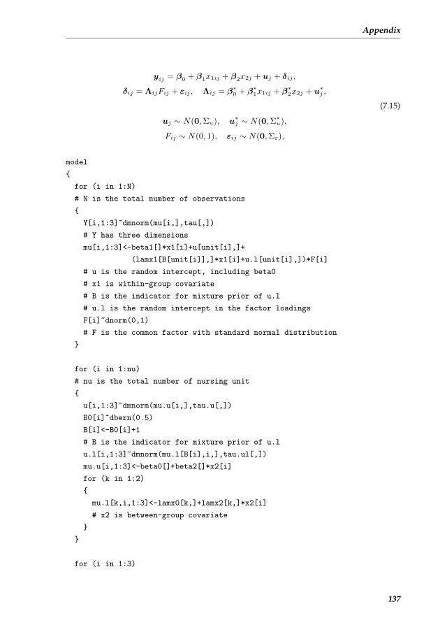
Appendix
yij = β0 + β1x1ij + β2x2j + uj + δij ,
δij = ΛijFij + εij , Λij = β∗0 + β∗1x1ij + β∗2x2j + u∗j ,
uj ∼ N(0,Σu), u∗j ∼ N(0,Σ∗u),
Fij ∼ N(0, 1), εij ∼ N(0,Σε),
(7.15)
model
{
for (i in 1:N)
# N is the total number of observations
{
Y[i,1:3]~dmnorm(mu[i,],tau[,])
# Y has three dimensions
mu[i,1:3]<-beta1[]*x1[i]+u[unit[i],]+
(lamx1[B[unit[i]],]*x1[i]+u.l[unit[i],])*F[i]
# u is the random intercept, including beta0
# x1 is within-group covariate
# B is the indicator for mixture prior of u.l
# u.l is the random intercept in the factor loadings
F[i]~dnorm(0,1)
# F is the common factor with standard normal distribution
}
for (i in 1:nu)
# nu is the total number of nursing unit
{
u[i,1:3]~dmnorm(mu.u[i,],tau.u[,])
B0[i]~dbern(0.5)
B[i]<-B0[i]+1
# B is the indicator for mixture prior of u.l
u.l[i,1:3]~dmnorm(mu.l[B[i],i,],tau.ul[,])
mu.u[i,1:3]<-beta0[]+beta2[]*x2[i]
for (k in 1:2)
{
mu.l[k,i,1:3]<-lamx0[k,]+lamx2[k,]*x2[i]
# x2 is between-group covariate
}
}
for (i in 1:3)
137
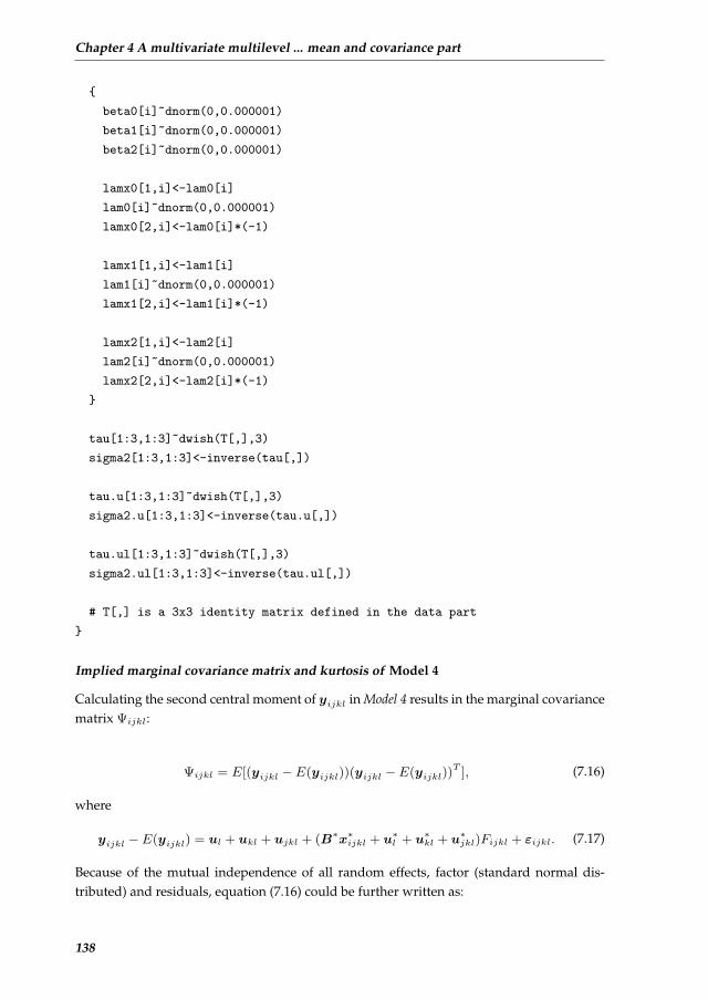
Chapter 4 A multivariate multilevel ... mean and covariance part
{
beta0[i]~dnorm(0,0.000001)
beta1[i]~dnorm(0,0.000001)
beta2[i]~dnorm(0,0.000001)
lamx0[1,i]<-lam0[i]
lam0[i]~dnorm(0,0.000001)
lamx0[2,i]<-lam0[i]*(-1)
lamx1[1,i]<-lam1[i]
lam1[i]~dnorm(0,0.000001)
lamx1[2,i]<-lam1[i]*(-1)
lamx2[1,i]<-lam2[i]
lam2[i]~dnorm(0,0.000001)
lamx2[2,i]<-lam2[i]*(-1)
}
tau[1:3,1:3]~dwish(T[,],3)
sigma2[1:3,1:3]<-inverse(tau[,])
tau.u[1:3,1:3]~dwish(T[,],3)
sigma2.u[1:3,1:3]<-inverse(tau.u[,])
tau.ul[1:3,1:3]~dwish(T[,],3)
sigma2.ul[1:3,1:3]<-inverse(tau.ul[,])
# T[,] is a 3x3 identity matrix defined in the data part
}
Implied marginal covariance matrix and kurtosis of Model 4
Calculating the second central moment of yijkl in Model 4 results in the marginal covariancematrix Ψijkl:
Ψijkl = E[(yijkl − E(yijkl))(yijkl − E(yijkl))T ], (7.16)
where
yijkl − E(yijkl) = ul + ukl + ujkl + (B∗x∗ijkl + u∗l + u∗kl + u∗jkl)Fijkl + εijkl. (7.17)
Because of the mutual independence of all random effects, factor (standard normal dis-tributed) and residuals, equation (7.16) could be further written as:
138
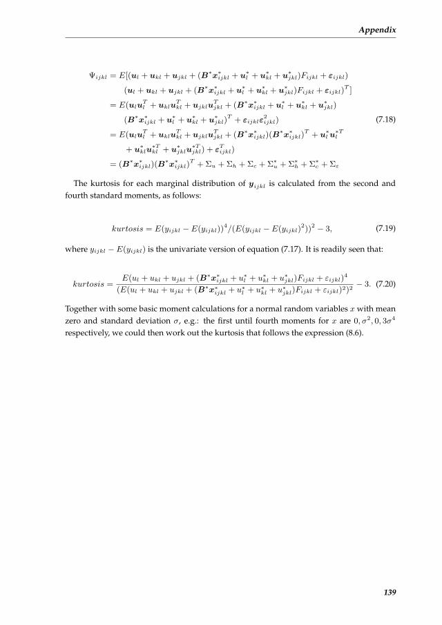
Appendix
Ψijkl = E[(ul + ukl + ujkl + (B∗x∗ijkl + u∗l + u∗kl + u∗jkl)Fijkl + εijkl)
(ul + ukl + ujkl + (B∗x∗ijkl + u∗l + u∗kl + u∗jkl)Fijkl + εijkl)T ]
= E(uluTl + uklu
Tkl + ujklu
Tjkl + (B∗x∗ijkl + u∗l + u∗kl + u∗jkl)
(B∗x∗ijkl + u∗l + u∗kl + u∗jkl)T + εijklε
2ijkl)
= E(uluTl + uklu
Tkl + ujklu
Tjkl + (B∗x∗ijkl)(B
∗x∗ijkl)T + u∗l u
∗Tl
+ u∗klu∗Tkl + u∗jklu
∗Tjkl) + εTijkl)
= (B∗x∗ijkl)(B∗x∗ijkl)
T + Σu + Σh + Σc + Σ∗u + Σ∗h + Σ∗c + Σε
(7.18)
The kurtosis for each marginal distribution of yijkl is calculated from the second andfourth standard moments, as follows:
kurtosis = E(yijkl − E(yijkl))4/(E(yijkl − E(yijkl)
2))2 − 3, (7.19)
where yijkl − E(yijkl) is the univariate version of equation (7.17). It is readily seen that:
kurtosis =E(ul + ukl + ujkl + (B∗x∗ijkl + u∗l + u∗kl + u∗jkl)Fijkl + εijkl)
4
(E(ul + ukl + ujkl + (B∗x∗ijkl + u∗l + u∗kl + u∗jkl)Fijkl + εijkl)2)2− 3. (7.20)
Together with some basic moment calculations for a normal random variables x with meanzero and standard deviation σ, e.g.: the first until fourth moments for x are 0, σ2, 0, 3σ4
respectively, we could then work out the kurtosis that follows the expression (8.6).
139


8MULTILEVEL HIGHER ORDER FACTOR
MODEL: JOINT MODELING OF AMULTILEVEL FACTOR ANALYTIC
MODEL AND A MULTILEVELCOVARIANCE REGRESSION MODEL
Chapter 8 is based on the paper:Li, B., Bruyneel, L., and Lesaffre, E. (2014). Multilevel higher-order factor model: Joint modeling ofa multilevel factor analytic model and a multilevel covariance regression model. Structural EquationModeling: A Multidisciplinary Journal. (submitted)
141
Chapter 8 Multilevel Higher Order Factor Model
Abstract
We propose a multilevel higher-order factor (MHOF) model that com-bines a multilevel factor analytic (MFA) model and a multilevel covari-ance regression (MCR) model, in a Bayesian context. The latter modelwas proposed by Li et al. (2013a) to express the covariance matrix of theresponses with a mixed effects structure via a factor analytic model withstructured factor loadings. The MHOF model replaces the responses inthe MCR part with the factor scores coming from an MFA model, whilepreserving the features of the MCR model. This is quite efficient whenthe responses of the MCR model are not measured directly but are latentvariables such as the burnout measurements in our example data set.
142
8.1 Introduction
8.1 Introduction
Factor analytic methods are commonly used to obtain insight into high-dimensional datastructures. When in addition the data have a multilevel structure, this hierarchical structureshould be incorporated into the factor analysis (Longford and Muthen, 1992). Modelinghigh-dimensional multivariate data can therefore become quite challenging, and becomeseven more demanding when some of the classical assumptions such as normality and ho-moscedasticity are not met. In a previous paper (Li et al., 2013a), we proposed a Bayesianmultivariate multilevel model with a built-in factor analytic model for the covariance matrix(also called the multilevel covariance regression, denoted as MCR) to handle a large four-level structured data set with a complex heteroscedastic structure with a three-dimensionalburnout response that has a non-normal but bounded distribution. The MCR approachproved to be a useful technique to get insight into this complex data structure.
Notwithstanding the complex nature of the data tackled in Li et al. (2013a), it was realizedthat the problem is even more complex. Indeed, the three-dimensional burnout vector wasobtained in the early 1980s through single-level factor models based on a relatively smallsample of US health and service occupation workers. From a preliminary list of 47 itemsmeasuring burnout, a 3-dimensional FA solution measured by 22 items emerged (Maslachand Jackson, 1981). To simplify the practical application of their 3-dimensional FA solu-tion, the authors suggested to use three sum scores of the original items representing thethree dimensions of the burnout measurements (Maslach et al., 1996). Although the di-mensions were labeled after the factor analysis rather than deduced theoretically (Schaufeliet al., 1993), this factor solution is generally supported (Worley et al., 2008). However, FAapproaches accounting for the multilevel research design that many researchers deploy, arenotably absent. The data set used in Li et al. (2013a) has a four-level structure: burnoutwas measured from nurses within nursing units in hospitals across 12 European countries.After taking into account this four-level structure the burnout dimensions may be differentfrom the solution suggested by Maslach and Jackson (1981). We therefore argue that theoriginal factor solution (and the resulting practical approach based on sum scores) obtainedby Maslach and Jackson (1981) may not apply to the RN4CAST population. It thus seemspreferable to evaluate the configural invariance of the three-factor burnout solution to theRN4CAST data, while taking into account the multilevel structure of these data. In addition,since the MCR model applied in Li et al. (2013a) revealed that the multilevel model basedon the sum scores showed heteroscedasticity in its covariance structure, it also seemed nec-essary to combine the multilevel FA (MFA) model with the MCR approach here. The aimof this paper is to jointly model an MCR and an MFA model with a Bayesian approach byusing the factor scores from the MFA model as the responses in the MCR model. We arguethat this approach overcomes several drawbacks associated with the use of sum scores.
There are typically two ways to combine the two models. The first is a two-stage ap-proach whereby the factor solutions are determined and then used as input for the MCRmodel. The second is a joint approach whereby the two estimation processes are performedsimultaneously. A comparison of these two approaches will be done here using a simulation
143

Chapter 8 Multilevel Higher Order Factor Model
study. Joint modeling of the MFA model and the MCR model results in a multilevel higher-order factor (MHOF) model. Basic ideas of a higher-order factor model can be found ine.g. Maruyama (1997). Here, we basically extend a complex higher-order factor structure tothe multilevel setting. The proposed MHOF model can be seen as a particular but complexexample of multilevel structural equation modeling (MSEM) (Muthen, 1994; Hox, 2010),but also as a multiple indicators multiple causes (MIMIC) model (Joreskog and Goldberger,1975). However, the structural part of our modeling (i.e. MCR) has, to our knowledge, notreceived attention in any MSEM or MIMIC model. Our modeling approach can handle thefollowing aspects simultaneously:
• multiple indicators with a multilevel structure;
• higher-order common factors;
• complex structured heteroscedasticity of the lower-order common factors.
We illustrate the MHOF model with the same unique RN4CAST data set that was used inLi et al. (2013a). Applying the joint model to the full multi-country set of RN4CAST data ishowever computationally demanding. But more importantly, the coefficients estimates andthe covariance pattern of burnout may vary across countries likely necessitating an evenmore complex statistical approach. We therefore applied the MHOF model to the Belgiandata only. The extension of our approach to the twelve countries will be the topic of interestin a subsequent paper with a more clinical focus.
The remainder of this paper is structured as follows. In Section 8.2, more details on themotivating data set are provided and the treatment of the non-responses and missing datais also elaborated. We specify the research questions that triggered the development of theMHOF model at the end of this section. The proposed MHOF model and its two compo-nents (MFA and MCR models) are introduced in Section 8.3. Computational details on fit-ting the models to data are discussed in Section 8.4. A limited simulation study to comparethe parameter estimates between the two-stage approach and the joint approach (MHOFmodel) is described in Section 8.5. Section 8.6 applies the proposed MHOF model to themotivating data set thereby addressing the research questions. The two-stage model andthe MCR model with sum scores as responses (proposed in Li et al. (2013a)) are also ap-plied here to make comparisons with the MHOF model. Several model assessments areperformed afterwards and a clinical interpretation of the parameter estimates is provided atthe end of the section. We conclude this paper with a summary of the significant advance-ments in statistical analyses resulting from the MHOF model.
8.2 Motivating Data set
8.2.1 Data description
We use the Belgian sample of the three-year RN4CAST nurse workforce study. The aimof this European FP7-funded project was to study the impact of system-level features inthe organization of nursing care on individual measures of nurse wellbeing and patient
144
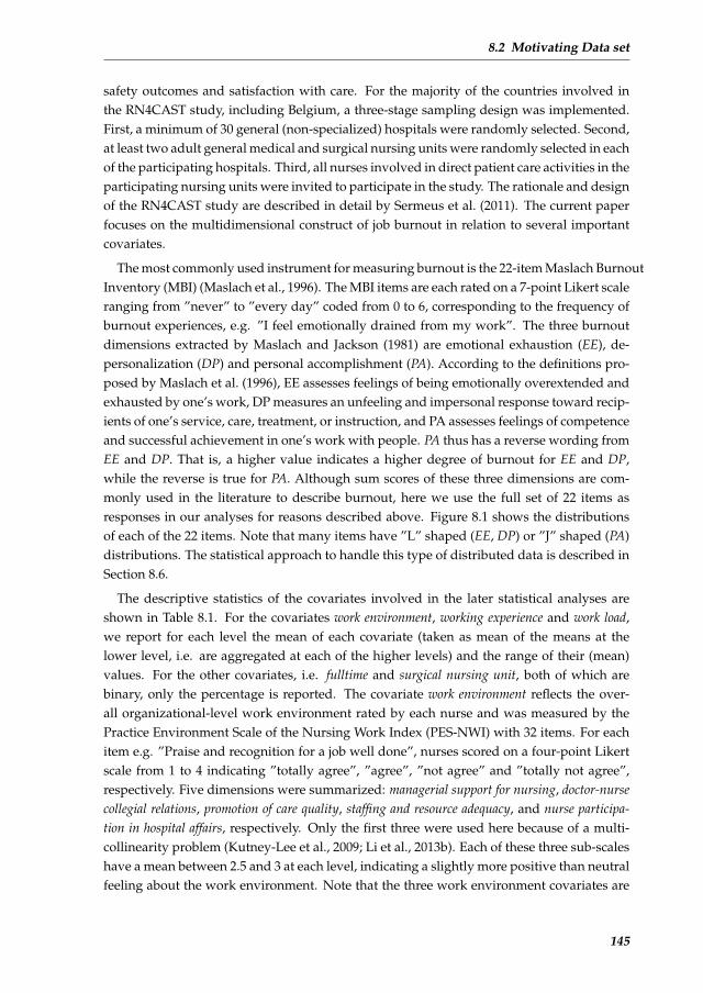
8.2 Motivating Data set
safety outcomes and satisfaction with care. For the majority of the countries involved inthe RN4CAST study, including Belgium, a three-stage sampling design was implemented.First, a minimum of 30 general (non-specialized) hospitals were randomly selected. Second,at least two adult general medical and surgical nursing units were randomly selected in eachof the participating hospitals. Third, all nurses involved in direct patient care activities in theparticipating nursing units were invited to participate in the study. The rationale and designof the RN4CAST study are described in detail by Sermeus et al. (2011). The current paperfocuses on the multidimensional construct of job burnout in relation to several importantcovariates.
The most commonly used instrument for measuring burnout is the 22-item Maslach BurnoutInventory (MBI) (Maslach et al., 1996). The MBI items are each rated on a 7-point Likert scaleranging from ”never” to ”every day” coded from 0 to 6, corresponding to the frequency ofburnout experiences, e.g. ”I feel emotionally drained from my work”. The three burnoutdimensions extracted by Maslach and Jackson (1981) are emotional exhaustion (EE), de-personalization (DP) and personal accomplishment (PA). According to the definitions pro-posed by Maslach et al. (1996), EE assesses feelings of being emotionally overextended andexhausted by one’s work, DP measures an unfeeling and impersonal response toward recip-ients of one’s service, care, treatment, or instruction, and PA assesses feelings of competenceand successful achievement in one’s work with people. PA thus has a reverse wording fromEE and DP. That is, a higher value indicates a higher degree of burnout for EE and DP,while the reverse is true for PA. Although sum scores of these three dimensions are com-monly used in the literature to describe burnout, here we use the full set of 22 items asresponses in our analyses for reasons described above. Figure 8.1 shows the distributionsof each of the 22 items. Note that many items have ”L” shaped (EE, DP) or ”J” shaped (PA)distributions. The statistical approach to handle this type of distributed data is described inSection 8.6.
The descriptive statistics of the covariates involved in the later statistical analyses areshown in Table 8.1. For the covariates work environment, working experience and work load,we report for each level the mean of each covariate (taken as mean of the means at thelower level, i.e. are aggregated at each of the higher levels) and the range of their (mean)values. For the other covariates, i.e. fulltime and surgical nursing unit, both of which arebinary, only the percentage is reported. The covariate work environment reflects the over-all organizational-level work environment rated by each nurse and was measured by thePractice Environment Scale of the Nursing Work Index (PES-NWI) with 32 items. For eachitem e.g. ”Praise and recognition for a job well done”, nurses scored on a four-point Likertscale from 1 to 4 indicating ”totally agree”, ”agree”, ”not agree” and ”totally not agree”,respectively. Five dimensions were summarized: managerial support for nursing, doctor-nursecollegial relations, promotion of care quality, staffing and resource adequacy, and nurse participa-tion in hospital affairs, respectively. Only the first three were used here because of a multi-collinearity problem (Kutney-Lee et al., 2009; Li et al., 2013b). Each of these three sub-scaleshave a mean between 2.5 and 3 at each level, indicating a slightly more positive than neutralfeeling about the work environment. Note that the three work environment covariates are
145

Chapter 8 Multilevel Higher Order Factor Model
0 1 2 3 4 5 6
Burnout item 1
020
040
060
0
0 1 2 3 4 5 6
Burnout item 2
Fre
quen
cy
020
040
060
0
0 1 2 3 4 5 6
Burnout item 3
Fre
quen
cy
010
030
050
0
0 1 2 3 4 5 6
Burnout item 4
Fre
quen
cy
040
080
012
00
0 1 2 3 4 5 6
Burnout item 5
Fre
quen
cy
040
080
012
00
0 1 2 3 4 5 6
Burnout item 6
050
010
0015
00
0 1 2 3 4 5 6
Burnout item 7
Fre
quen
cy
040
080
012
00
0 1 2 3 4 5 6
Burnout item 8
Fre
quen
cy
020
040
060
080
0
0 1 2 3 4 5 6
Burnout item 9
Fre
quen
cy
020
040
060
080
0
0 1 2 3 4 5 6
Burnout item 10
Fre
quen
cy
050
010
0015
00
0 1 2 3 4 5 6
Burnout item 11
020
060
010
00
0 1 2 3 4 5 6
Burnout item 12
Fre
quen
cy
020
040
060
080
0
0 1 2 3 4 5 6
Burnout item 13
Fre
quen
cy
020
040
060
0
0 1 2 3 4 5 6
Burnout item 14
Fre
quen
cy
010
030
050
0
0 1 2 3 4 5 6
Burnout item 15
Fre
quen
cy
050
010
0020
00
0 1 2 3 4 5 6
Burnout item 16
020
060
0
0 1 2 3 4 5 6
Burnout item 17
Fre
quen
cy
020
060
010
00
0 1 2 3 4 5 6
Burnout item 18
Fre
quen
cy
020
060
010
00
0 1 2 3 4 5 6
Burnout item 19
Fre
quen
cy
020
060
010
00
0 1 2 3 4 5 6
Burnout item 20
Fre
quen
cy
020
040
060
080
0
0 1 2 3 4 5 6
Burnout item 21
020
040
060
080
0
0 1 2 3 4 5 6
Burnout item 22
Fre
quen
cy
020
060
010
00
Figure 8.1: Bar plot for each of the 22 burnout items.
146
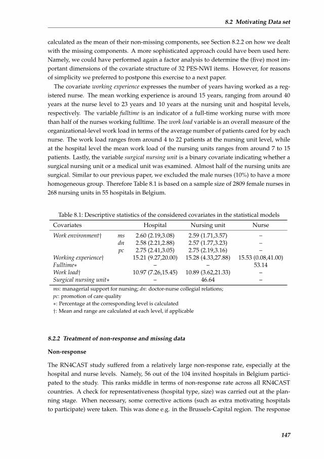
8.2 Motivating Data set
calculated as the mean of their non-missing components, see Section 8.2.2 on how we dealtwith the missing components. A more sophisticated approach could have been used here.Namely, we could have performed again a factor analysis to determine the (five) most im-portant dimensions of the covariate structure of 32 PES-NWI items. However, for reasonsof simplicity we preferred to postpone this exercise to a next paper.
The covariate working experience expresses the number of years having worked as a reg-istered nurse. The mean working experience is around 15 years, ranging from around 40years at the nurse level to 23 years and 10 years at the nursing unit and hospital levels,respectively. The variable fulltime is an indicator of a full-time working nurse with morethan half of the nurses working fulltime. The work load variable is an overall measure of theorganizational-level work load in terms of the average number of patients cared for by eachnurse. The work load ranges from around 4 to 22 patients at the nursing unit level, whileat the hospital level the mean work load of the nursing units ranges from around 7 to 15patients. Lastly, the variable surgical nursing unit is a binary covariate indicating whether asurgical nursing unit or a medical unit was examined. Almost half of the nursing units aresurgical. Similar to our previous paper, we excluded the male nurses (10%) to have a morehomogeneous group. Therefore Table 8.1 is based on a sample size of 2809 female nurses in268 nursing units in 55 hospitals in Belgium.
Table 8.1: Descriptive statistics of the considered covariates in the statistical models
Covariates Hospital Nursing unit Nurse
Work environment† ms 2.60 (2.19,3.08) 2.59 (1.71,3.57) –dn 2.58 (2.21,2.88) 2.57 (1.77,3.23) –pc 2.75 (2.41,3.05) 2.75 (2.19,3.16) –
Working experience† 15.21 (9.27,20.00) 15.28 (4.33,27.88) 15.53 (0.08,41.00)Fulltime∗ – – 53.14Work load† 10.97 (7.26,15.45) 10.89 (3.62,21.33) –Surgical nursing unit∗ – 46.64 –ms: managerial support for nursing; dn: doctor-nurse collegial relations;pc: promotion of care quality∗: Percentage at the corresponding level is calculated†: Mean and range are calculated at each level, if applicable
8.2.2 Treatment of non-response and missing data
Non-response
The RN4CAST study suffered from a relatively large non-response rate, especially at thehospital and nurse levels. Namely, 56 out of the 104 invited hospitals in Belgium partici-pated to the study. This ranks middle in terms of non-response rate across all RN4CASTcountries. A check for representativeness (hospital type, size) was carried out at the plan-ning stage. When necessary, some corrective actions (such as extra motivating hospitalsto participate) were taken. This was done e.g. in the Brussels-Capital region. The response
147

Chapter 8 Multilevel Higher Order Factor Model
rate at the individual nurse level was 72.07%, which is higher than the average response rate(60.2%) in the RN4CAST study. Since no information is available on the non-respondents,no corrective actions for non-response could be undertaken at the analysis stage. However,in a similar nurse survey conducted in the US (Smith, 2008), the author assessed the non-response bias by randomly selecting a number of non-respondents and motivating themto fill in the questionnaires. No differences were found with regard to nurses’ assessmentsof their work environment and burnout. Therefore we argue our findings are likely notdramatically affected by the non-response data.
Missingness in the burnout measurements
There are about 10% nurses having at least one of the 22 burnout items missing. Technically,missing responses are easily dealt with using the Markov Chain Monte Carlo (MCMC) tech-nique in Bayesian modeling. For instance, with WinBUGS the missing response needs to beindicated by ‘NA’. In the MCMC iterative procedure, the missing response is then automati-cally imputed at each iteration, thereby actually performing a multiple imputation approachat convergence. Here it implies that for each iteration, the missing values of the 22 items areimputed via the likelihood based on the current parameter estimates and will be involvedin the estimation of parameters for the next iteration. To this end, the parameter estimatesare actually based on the observed and the multiple imputed data.
Missingness in covariates
We first note that the three work environment covariates are calculated as the mean of theirnon-missing components. Hence, when some of the components are missing they are nottaken into account into the mean score. This assumes a too simple missing-data pattern, ac-tually missing completely at random. For all covariates in Table 8.1, only working experienceand fulltime have missing values with the missing rates about 11% and 1%, respectively. Tomaximally exploit the data set, we applied a Bayesian imputation scheme for each covariate.But this now also requires a statistical model for the joint distribution of the two covariates.Ibrahim et al. (2002) pointed out that the joint model specification is problematic when boththe categorical and continuous covariates have missing values, which is the case here forsome of the observations. This is one of the the motivations for them to come up with thesolution for the joint distribution a sequence of one-dimensional conditional distributions.Applying this to our situation, which is much simpler with only two covariates that haveoccasionally missing data, implies that p(x1, x2 | ψ, . . .) = p(x1 | x2, ψ1, . . .)p(x2 | ψ2, . . .).That is, the joint distribution of the two covariates is written as the product of two con-ditional distributions with x1 and x2 the working experience and fulltime, respectively and. . . signifies that other covariates are included in the model specification. ψ representsall parameters involved in the joint distribution which could be divided into ψ1 and ψ2
belonging to the two conditional models, respectively. For the conditional distributionp(x1 | x2, ψ1, . . .) we assumed a Gaussian linear model for x1 with regressors all covari-ates in Table 8.1 (hence including fulltime). The conditional distribution p(x2 | ψ2, . . .) has
148

8.3 Proposed model
a logistic regression model with again all complete covariates as predictors. Obviously, theparameters of the two conditional distributions must be estimated using only the subjectswith non-missing regressor values in their respective model. A more detailed specificationof the models can be found in the Supplementary Materials 1. Finally, the parameters of thetwo conditional imputation models are estimated simultaneously with the MHOF modelfor the burnout responses.
8.2.3 Research questions
In this paper we wish to examine three research questions related to the burnout measure-ments. We believe that the MHOF model developed in the next section in combination withthe large RN4CAST data set will allow us to address these questions appropriately. Ourresearch questions are:
• Is there any evidence of configural invariance/ non-invariance (Steenkamp and Baum-gartner, 1998) comparing the factor structure of the current data set with the one pro-posed by Maslach and Jackson (1981)? That is, we wish to evaluate whether the twofactor structures are the same in terms of the number of common factors and the itemswithin each common factor dimension.
• Are the means of the latent burnout dimensions (factor solutions) correlated with theorganizational-level and individual-level characteristics?
• Are the correlations among the latent burnout dimensions stable across hospitals,nursing units and nurses, after taking into account a rich set of confounders at dif-ferent levels?
The first research question involves a multilevel FA model based on the original 22 burnoutitems. We will however show that for all three research questions the MHOF model isneeded.
8.3 Proposed model
The Multilevel Higher-Order Factor (MHOF) model contains two parts as illustrated in Fig-ure 8.2: an MFA model and an MCR model. In this section, we first describe these twocomponents and then combine them to establish the MHOF model. To simplify matters, weassume in this section that in all models the responses are normally distributed. In Section8.6 we explain how we dealt with non-normality of the 22 items in the RN4CAST study.
8.3.1 Multilevel factor analytic (MFA) model
The factor model aims to summarize a (large) number of measurements with a limited set of(latent) variables (called common factors) thereby preserving most of the original informa-tion. The MFA model is a multilevel version of the classical confirmatory factor model, see
1All Supplementary materials in this chapter can be found in the website where it is published.
149

Chapter 8 Multilevel Higher Order Factor Model
Hox (2010) and Goldstein (2010) for a general and detailed description of the MFA model.Our motivating data set has a three-level structure, i.e. nurses within nursing units withinhospitals, implying a three-level factor model. Since our interest lies in further modeling ofthe nurse-level common factors, we estimate an unstructured covariance matrix at the nurs-ing unit level and hospital level respectively and keep only the nurse-level factor structure.The considered three-level factor model is therefore:
yijk = µ+ bjk + bk + Lzijk + εijk,
bjk ∼ N(0,Σbu), bk ∼ N(0,Σbh), zijk ∼ N(0,Σz),
εijk ∼ N(0, diag(σ21 , σ
22 , . . . , σ
2P )),
(8.1)
where yijk represents the P = 22-dimensional response for nurse i in nursing unit j in hos-pital k; zijk is the Q-dimensional nurse-level common factor following a multivariate nor-mal distribution with an unstructured covariance matrix Σz , andL is its P ×Q-dimensionalloading matrix; bjk and bk represent the higher-level random effects with an unstructuredcovariance matrix Σbu and Σbh respectively. εijk represents the nurse-level P -dimensionalresidual having a normal distribution with mean zero and variance σ2
p for each of its Pelements. The unique factors are assumed to be independent with each other at each levelrespectively for the sake of identification. This will be elaborated in Section 8.3.4. The upperpart of Figure 8.2 displays graphically model (8.1).
8.3.2 Multilevel covariance regression (MCR) model
The covariance regression model was first proposed by Hoff and Niu (2012) with a multi-variate regression model that has a built-in factor analytic model with factor loadings hav-ing a linear model. The covariance matrix of the multivariate responses, determined by thefactor part, depends quadratically on covariates. The MCR model extends Hoff and Niu’scovariance regression model into the multilevel situation. In an MCR model, both the meanand the covariance parts are allowed to have a mixed effects model and can be modeledsimultaneously. In Li et al. (2013a), a Bayesian approach was opted, as here, for estimatingthe parameters. The authors showed that this approach performed well on the RN4CASTdata.
The MCR model for the Belgian data of the RN4CAST project is given by:
zijk = Bxijk + ujk + uk + δijk,
δijk = ΛijkFijk + εijk, Λijk = B∗x∗ijk + u∗jk + u∗k,
ujk ∼ N(0,Σu), uk ∼ N(0,Σh),
u∗jk ∼ N(0,Σ∗u), u∗k ∼ N(0,Σ∗h),
Fijk ∼ N(0, 1), εijk ∼ N(0,Σε),
(8.2)
where zijk is the Q-dimensional latent burnout variables for nurse i in nursing unit j inhospital k; B is a Q × m matrix of fixed effects associated with the m-dimensional vectorxijk gathering information from all levels. ujk and uk represent theQ-dimensional random
150

8.3 Proposed model
Figure 8.2: The MHOF model: The upper part describes the MFA model, which is a three-level factor analytic model and the lower part describes the MCR part, whichis a three-level covariance regression model with the factor loadings having amixed effects structure. A square represents an observed response or covariate.A circle represents a latent variable. L1-L3 represent the loadings of F1-F3 on Frespectively. A unidirectional arrow connecting two objects represents a regres-sion relationship, and a bidirectional arrow connecting two objects represents thecorrelation of the two objects. A small arrow pointed to a single object representsthe estimation of the error term and the multiple arrows at the nursing unit andhospital levels represent the estimation of the general covariance matrix at eachlevel respectively. The arrows with gray color represent the cross loadings.
intercepts in the mean part at each higher level with general covariance matrices Σu and Σh,respectively. The residuals δijk are decomposed into a fixed part assumed constant acrossnurses with general covariance matrix Σε and a part that varies withm∗ characteristics x∗ijkpossibly different from xijk and allowed to depend on all levels through a factor part. B∗
is a Q ×m∗ matrix of fixed effects associated with x∗ijk, while u∗jk and u∗k represent the Q-dimensional random intercepts in the loadings at each higher level with general covariancematrices Σ∗u and Σ∗h, respectively. The lower part of Figure 8.2 displays graphically model(8.2).
8.3.3 Multilevel higher-order factor (MHOF) model
The MHOF model is a combination of an MFA and an MCR model. The combination isrealized by letting the common factors serve both as the latent variables in the MFA part,as well as dependent variables in the MCR part. Figure 8.2 shows graphically how theMFA and MCR models are combined into the MHOF model. The MHOF model is formally
151

Chapter 8 Multilevel Higher Order Factor Model
defined as:
The MFA part :
yijk = µ+ bjk + bk + Lzijk + εFAijk ,
bjk ∼ N(0,Σbu), bk ∼ N(0,Σbh),
εFAijk ∼ N(0, diag(σ21 , σ
22 , . . . , σ
2P )).
The MCR part :
zijk = Bxijk + δijk,
δijk = ΛijkFijk + εCRijk , Λijk = B∗x∗ijk + u∗jk + u∗k,
u∗jk ∼ N(0,Σ∗u), u∗k ∼ N(0,Σ∗h),
Fijk ∼ N(0, 1), εCRijk ∼ N(0,Σε).
(8.3)
The MFA part is the same as in model (8.1) except for the distribution of zijk, which isincorporated in the MCR model later on. We refer to it as the lower-order factor in theMHOF model. The zijk in the MCR part are output from the MFA model. All parametershave the same meaning as in model (8.2) except that now the random effects at the nursingunit and hospital levels in the mean, i.e. ujk and uk, have been removed for identificationpurposes discussed in Section 8.3.4. The common factors Fijk are also called the higher-order factors in the MHOF model.
Model (8.3) could be also written in a compact form as:
yijk = µ+ bjk + bk + LBxijk + L(B∗x∗ijk + u∗jk + u∗k)Fijk + LεCRijk + εFAijk ,
bjk ∼ N(0,Σbu), bk ∼ N(0,Σbh), εFAijk ∼ N(0, diag(σ21 , σ
22 , . . . , σ
2P )).
u∗jk ∼ N(0,Σ∗u), u∗k ∼ N(0,Σ∗h), Fijk ∼ N(0, 1), εCRijk ∼ N(0,Σε).
(8.4)
From this expression we can see that the nursing unit and hospital level-specific randomintercepts, i.e. bjk and bk, have a multivariate normal distribution with a general covariancematrix, respectively. This is already a saturated model for the covariance matrix at each ofthe two levels, which prevents the inclusion of any other kinds of random effects at theselevels to the mean of the observed P-dimensional responses, and thus to the mean of zijk.We will come back to this in the next section on identification issues.
The MCR model expresses the covariances through a single factor structure whereby thefactor loadings are assumed to be random and modeled with a mixed effects structure. Thecovariance matrix built by the factor loadings then has a mixed effects structure accordingly,and the implied marginal covariance matrix for the latent common factors is given by:
Ψijk = (B∗x∗ijk)(B∗x∗ijk)T + Σ∗u + Σ∗h + Σε. (8.5)
Note that in our example the dimension of the response in the MCR model isQ = 3 and thatthe marginal covariance matrices Ψijk span the whole of the 3× 3 matrices at each value ofx∗ijk.
152

8.3 Proposed model
Similar as in Li et al. (2013a), we can prove that the marginal distribution for each of thethree common factors is not normal. While for each marginal density, the skewness is stillzero when all random effects are mutually independent(assumed here), the kurtosis for theqth marginal density of the lower-order factor becomes:
kurtosisq =6a∗2q + 12a∗qbq
(a∗q + bq + cq)2. (8.6)
In expression (8.6), a∗q , bq , cq are the qth diagonal elements of (Σ∗u+Σ∗h), (B∗x∗ijk)(B∗x∗ijk)T
and Σε, respectively. From this expression we can conclude that the marginal densities areleptokurtic unless the variance of the random effects in the factor loadings is zero (a∗q = 0),and that the kurtosis also depends on the covariates in the factor loadings.
8.3.4 Identification issues
There are three main identification concerns for the MHOF model, coming from the MFApart, the MCR part, and the joint modeling of these two models. We describe these one byone.
Firstly, for the MFA part, it is well-known that scaling constraints are necessary, for eitherthe loading parameters or the variances of the common factors. Here we scaled the loadingparameters of the lower-order factors zijk. A common way is to set the first loading foreach common factor to a constant value, usually 1, see, e.g. Kline (2010). Cross-loadingsare in practice most often small but non-zero, that is why we estimated them as well. This,however, violates the rule of having at least Q2 constraints in a frequentist factor analyticmodel, see e.g. Asparouhov and Muthen (2009). For the Bayesian approach informativepriors for the cross-loadings can restrict them stochastically and thereby overcoming theidentification problem. This was called Bayesian structural equation modeling (BSEM) byMuthen and Asparouhov (2012). The largest cross-loading estimates obtained by Maslachand Jackson (1981) were close to 0.4. Therefore we have chosen an informative normalprior with mean zero and standard deviation around 0.22 for all cross-loadings. This choicecorresponds to a 95% prior range of the cross loadings from -0.45 to 0.45 and allowed thefactor loadings to be identified. In addition we assumed that theP unique factors (residuals)are mutually independent.
Secondly, for the MCR part, the identification issue is the same as described in the paperby Li et al. (2013a). That is, we scaled the higher-order factors with a standard normal distri-bution, and assigned a mixture prior for the random effects u∗jk and u∗k and the coefficientB∗ respectively to overcome the ”flipping states” issue. Given a reasonable variation ofx∗ijk, all parameters in the MCR part, including the whole covariance matrix of the residualεCRijk , could be identified.
The final identification issue stems from the joint modeling of the MFA and the MCRparts. As described above, the key part of this joint modeling are the lower-order factors thatconnect the MFA part and the MCR part. From the MHOF model expressed in both models(8.3) and (8.4), the nursing unit and hospital level-specific covariance matrices formulated
153

Chapter 8 Multilevel Higher Order Factor Model
by bjk and bk, respectively, are saturated, therefore adding random effects to the lower-order factor scores zijk, which will further contribute to the saturated covariance matricesat higher levels, cannot be identified. For this reason we did not include the random effects(ujk and uk) when modeling the mean of burnout (i.e. the lower-order factor scores zijk).There is no such constraint for the modeling the variance/covariance of the factor scores, i.e.modeling the heteroscedasticity. It is valid to assume that the variance of burnout withineach nursing unit is different and may also depend on some covariates. That is also tosay that the modeling of the (co)variance of the lower-level factor(s) could be multilevelstructured, even when the modeling of the mean structure does not have a hierarchicalstructure. We refer to the paper of Li et al. (2013a) for more details on the MCR model.
8.4 Computational procedure
We have opted for the Bayesian approach, for a variety of reasons. One is that the con-sidered model has a relatively large number of random effects, which is known to causeproblems in maximum likelihood algorithms. For the three-level MHOF model, there are2P random intercepts for the P indicators,Q lower-order common factors, one higher-ordercommon factor, and two extra random intercepts for each of the Q factor loadings for thehigher-order common factor. For our analyses, the Jags (Just another Gibbs sampler) MCMCprogram (Plummer, 2003) was used through the R package rjags (Plummer, 2013). We ran50,000 iterations for the burn-in part and another 50,000 iterations for model estimation. TheBrooks-Gelman-Rubin plots with the potential scale reduction factor (Brooks and Gelman,1998) (PSRF, which should be smaller than 1.1) was used for convergence checking. In ad-dition, we ran the Markov chain until the Monte Carlo error was around or smaller than 5%of the posterior standard deviation.
In a Bayesian analysis, all parameters need a prior distribution to express what was al-ready known beforehand. Reasonable informative priors can lead to more accurate param-eter estimates, which is one of the benefits of using the Bayesian approach. Here we usedinformative priors for the cross-loadings of the lower-order factors to overcome the identifi-cation issue described in Section 8.3.4. For the other loading parameters and the intercepts,a vague normal distribution was used for each with mean zero and a large variance (106).For the variance/covariance parameters, we used a inverse gamma distribution with smallshape and rate parameters (0.001) for the univariate case. For the multivariate case we usedan inverse Wishart distribution with a small scale matrix (0.01I with I the identity matrix)and degrees of freedom equal to the dimension of the matrix. For the MCR part, all pa-rameters (including the variance/covariance parameters and the rest) have the same vaguenormal distribution or inverse gamma/Wishart distribution as for the MFA part, except forthe mixture priors of some of the loading parameters (see above).
Models were compared using a pseudo Bayes factor (PSBF), see e.g. Lesaffre and Lawson(2012) for details on the computation. The classical criteria such as DIC (Spiegelhalter et al.,2002), though theoretically feasible for the BOS approach (see Section 8.6), is practicallycumbersome as the BOS approach requires an integration for each observation. In Li et al.
154
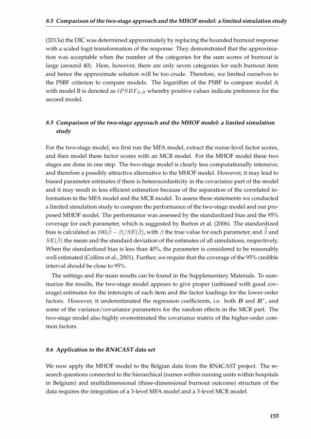
8.5 Comparison of the two-stage approach and the MHOF model: a limited simulation study
(2013a) the DIC was determined approximately by replacing the bounded burnout responsewith a scaled logit transformation of the response. They demonstrated that the approxima-tion was acceptable when the number of the categories for the sum scores of burnout islarge (around 40). Here, however, there are only seven categories for each burnout itemand hence the approximate solution will be too crude. Therefore, we limited ourselves tothe PSBF criterion to compare models. The logarithm of the PSBF to compare model Awith model B is denoted as `PSBFA,B whereby positive values indicate preference for thesecond model.
8.5 Comparison of the two-stage approach and the MHOF model: a limited simulationstudy
For the two-stage model, we first run the MFA model, extract the nurse-level factor scores,and then model these factor scores with an MCR model. For the MHOF model these twostages are done in one step. The two-stage model is clearly less computationally intensive,and therefore a possibly attractive alternative to the MHOF model. However, it may lead tobiased parameter estimates if there is heteroscedasticity in the covariance part of the modeland it may result in less efficient estimation because of the separation of the correlated in-formation in the MFA model and the MCR model. To assess these statements we conducteda limited simulation study to compare the performance of the two-stage model and our pro-posed MHOF model. The performance was assessed by the standardized bias and the 95%coverage for each parameter, which is suggested by Burton et al. (2006). The standardizedbias is calculated as 100| ¯β − β|/SE(β), with β the true value for each parameter, and ¯
β andSE(β) the mean and the standard deviation of the estimates of all simulations, respectively.When the standardized bias is less than 40%, the parameter is considered to be reasonablywell estimated (Collins et al., 2001). Further, we require that the coverage of the 95% credibleinterval should be close to 95%.
The settings and the main results can be found in the Supplementary Materials. To sum-marize the results, the two-stage model appears to give proper (unbiased with good cov-erage) estimates for the intercepts of each item and the factor loadings for the lower-orderfactors. However, it underestimated the regression coefficients, i.e. both B and B∗, andsome of the variance/covariance parameters for the random effects in the MCR part. Thetwo-stage model also highly overestimated the covariance matrix of the higher-order com-mon factors.
8.6 Application to the RN4CAST data set
We now apply the MHOF model to the Belgian data from the RN4CAST project. The re-search questions connected to the hierarchical (nurses within nursing units within hospitalsin Belgium) and multidimensional (three-dimensional burnout outcome) structure of thedata requires the integration of a 3-level MFA model and a 3-level MCR model.
155

Chapter 8 Multilevel Higher Order Factor Model
8.6.1 Choice of response and covariates
The ”L” and ”J” shaped distributions in Figure 8.1 require some advanced modeling ap-proach. Well ordinal logistic or probit modeling may be considered, we opted here foranother technique to handle these bounded outcome scores (BOS). We follow here the ap-proach suggested by Lesaffre et al. (2007). This assumes that a standardized version ofthe burnout measurement is a coarsened latent continuous variable which has a Gaussiandistribution after a logit transformation. More specifically, the observed response is firsttransformed to a (discrete) response y on the unit interval (by a change of scale). Then, a la-tent random variable z on (0,1) is assumed, with the property that log[z/(1− z)] ∼ N(µ, σ2)
and such that y is obtained by coarsening z. Lesaffre et al. (2007) showed that this approachcan handle well a large variety of distributions defined on a finite interval. In our analysis,we applied this technique to all 22 burnout items.
The candidate covariates involved in the mean and/or variance structures in later anal-yses, are listed in Table 8.1. In order to make the regression coefficients of these variablescomparable and to improve computational properties, standardized covariates (mean=0,SD=1) were used in later analyses. In addition, in order to investigate the level-specific ef-fects of the covariates, the following decomposition was made, as suggested by Neuhausand Kalbfleisch (1998):
xijk = (xijk − xjk) + (xjk − xk) + xk
= xn + xu + xh,(8.7)
xjk = 1njk
∑njk
i=1 xijk and xk = 1nk
∑nki=1 xjk. In expression (8.7), the lowest level variable is
partitioned into three parts corresponding to the three levels, i.e. n for nurse, u for nursingunit and h for hospital. By doing so, we study the ”pure” effect of the covariates at each level(for work environment and work load, there is no nurse-level partition because the lowest levelmeasurement is nursing unit).
8.6.2 An exploratory MFA model
Before we fitted the MHOF model, an exploratory MFA was conducted to explore the factorstructure of the 22 Maslach items, thereby addressing the first research question in Sec-tion 8.2. This analysis will also hint towards an appropriate MFA part of the MHOF model.Mplus v7 (Muthen and Muthen, 2010) was used for this task, making use of the robust maxi-mum likelihood estimator (Asparouhov and Muthen, 2005) and an oblique rotation method.As a result, the three-factor solution based on the eigenvalues (larger than 1) summarizesthe 22 items relatively well with reasonable RMSEA (0.027), and SRMR (0.027) values. RM-SEA represents the root mean square error of approximation, with a value of smaller than0.06 being considered good fit (Hu and Bentler, 1999). SRMR is the standardized root meansquare residual with a value smaller than 0.08 representing a good fit (Hu and Bentler, 1999).We found that the configuration of the nurse-level factor structure is similar as in Maslachand Jackson (1981), i.e. with similar three factors EE, DP and PA having similar theoreticalmeanings as before, but with two major discrepancies besides some minor differences in the
156
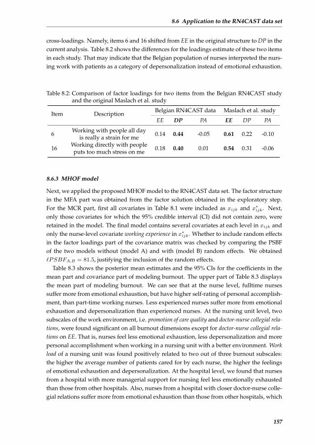
8.6 Application to the RN4CAST data set
cross-loadings. Namely, items 6 and 16 shifted from EE in the original structure to DP in thecurrent analysis. Table 8.2 shows the differences for the loadings estimate of these two itemsin each study. That may indicate that the Belgian population of nurses interpreted the nurs-ing work with patients as a category of depersonalization instead of emotional exhaustion.
Table 8.2: Comparison of factor loadings for two items from the Belgian RN4CAST studyand the original Maslach et al. study
Item Description Belgian RN4CAST data Maslach et al. study
EE DP PA EE DP PA
6 Working with people all day 0.14 0.44 -0.05 0.61 0.22 -0.10is really a strain for me
16 Working directly with people 0.18 0.40 0.01 0.54 0.31 -0.06puts too much stress on me
8.6.3 MHOF model
Next, we applied the proposed MHOF model to the RN4CAST data set. The factor structurein the MFA part was obtained from the factor solution obtained in the exploratory step.For the MCR part, first all covariates in Table 8.1 were included as xijk and x∗ijk. Next,only those covariates for which the 95% credible interval (CI) did not contain zero, wereretained in the model. The final model contains several covariates at each level in xijk andonly the nurse-level covariate working experience in x∗ijk. Whether to include random effectsin the factor loadings part of the covariance matrix was checked by comparing the PSBFof the two models without (model A) and with (model B) random effects. We obtained`PSBFA,B = 81.5, justifying the inclusion of the random effects.
Table 8.3 shows the posterior mean estimates and the 95% CIs for the coefficients in themean part and covariance part of modeling burnout. The upper part of Table 8.3 displaysthe mean part of modeling burnout. We can see that at the nurse level, fulltime nursessuffer more from emotional exhaustion, but have higher self-rating of personal accomplish-ment, than part-time working nurses. Less experienced nurses suffer more from emotionalexhaustion and depersonalization than experienced nurses. At the nursing unit level, twosubscales of the work environment, i.e. promotion of care quality and doctor-nurse collegial rela-tions, were found significant on all burnout dimensions except for doctor-nurse collegial rela-tions on EE. That is, nurses feel less emotional exhaustion, less depersonalization and morepersonal accomplishment when working in a nursing unit with a better environment. Workload of a nursing unit was found positively related to two out of three burnout subscales:the higher the average number of patients cared for by each nurse, the higher the feelingsof emotional exhaustion and depersonalization. At the hospital level, we found that nursesfrom a hospital with more managerial support for nursing feel less emotionally exhaustedthan those from other hospitals. Also, nurses from a hospital with closer doctor-nurse colle-gial relations suffer more from emotional exhaustion than those from other hospitals, which
157
Chapter 8 Multilevel Higher Order Factor Model
seems somewhat illogical. We come back to this in the clinical interpretation part. Work loadof a hospital was found positively related to emotional exhaustion.
The lower part of Table 8.3 displays the covariance part of modeling burnout. We can seethat experienced nurses have a larger variation of self-rating of personal accomplishmentthan less experienced nurses. A clinical interpretation of these results is given in Section8.6.7. Figure 8.3 shows the relationships between the (co)variances/correlations amongthe three burnout dimensions with the variable working experience at the nurse level. All(co)variances/correlations remained almost constant with working experience except for thevariance of personal accomplishment, which changed significantly with working experience,from around 0.7 for the unexperienced nurses to around 1.5 for the most experienced nurses.We did not find any significant covariates that could explain the variation of the variancesof burnout at the hospital and nursing unit levels. Therefore the variation of the variancescan only be ‘explained’ by the random effects. The variance estimates of the random effectsare similar at these two levels for each of the three burnout dimensions respectively, whichare around 0.15, 0.21 and 0.13 for emotional exhaustion, depersonalization and personalaccomplishment, respectively.
8.6.4 Comparison with the two-stage model
We compared the final MHOF model with the parameter estimates obtained from a two-stage analysis. The MFA model is based on the factor solution from Section 8.6.2. For theMCR model, the variables selection strategy was identical as before.
We found that, for the two-stage model and the MHOF model, the same covariates showedsignificant effects on the mean modeling of burnout at the nurse and nursing unit levels. Atthe hospital level, however, no covariates were found to be significantly associated to anyof the burnout dimensions for the two-stage model, while three covariates were found tobe significant in the MHOF model. In the covariance part, both models found only the co-variate working experience to be significantly associated to PA. With regard to the magnitudeof the parameter estimates, we found that the two-stage model provided smaller estimatesthan the MHOF model, which was in line with what we found through the simulation study.A more detailed list of the parameter estimates of the two models was given in the Supple-mentary Materials. In conclusion, for our motivating data set, the MHOF model seemed toshow more power and efficiency for the parameter estimates.
8.6.5 Comparison with the MCR model using sum scores
In this section we compare the parameter estimates obtained from the MHOF model withthose obtained from the MCR model with the sum scores (defined in Maslach et al. (1996)) asthe responses. The use of sum scores can be criticized because it does not adjust for differentweighting of the individual items, but rather assume equal contributions of the items. Thesum scores are also assumed to be mutually exclusive while in reality, the cross-loadings(often relatively small) are quite common. That is, one item could contribute to more thanone sum scores (DiStefano et al., 2009). We now wished to see whether the results obtained
158
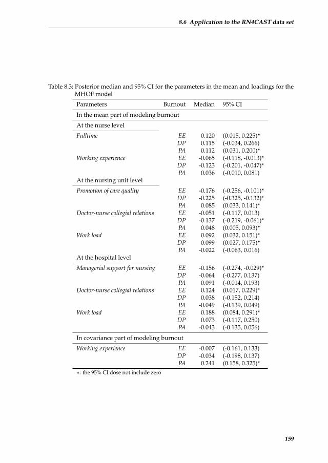
8.6 Application to the RN4CAST data set
Table 8.3: Posterior median and 95% CI for the parameters in the mean and loadings for theMHOF model
Parameters Burnout Median 95% CI
In the mean part of modeling burnout
At the nurse level
Fulltime EE 0.120 (0.015, 0.225)*DP 0.115 (-0.034, 0.266)PA 0.112 (0.031, 0.200)*
Working experience EE -0.065 (-0.118, -0.013)*DP -0.123 (-0.201, -0.047)*PA 0.036 (-0.010, 0.081)
At the nursing unit level
Promotion of care quality EE -0.176 (-0.256, -0.101)*DP -0.225 (-0.325, -0.132)*PA 0.085 (0.033, 0.141)*
Doctor-nurse collegial relations EE -0.051 (-0.117, 0.013)DP -0.137 (-0.219, -0.061)*PA 0.048 (0.005, 0.093)*
Work load EE 0.092 (0.032, 0.151)*DP 0.099 (0.027, 0.175)*PA -0.022 (-0.063, 0.016)
At the hospital level
Managerial support for nursing EE -0.156 (-0.274, -0.029)*DP -0.064 (-0.277, 0.137)PA 0.091 (-0.014, 0.193)
Doctor-nurse collegial relations EE 0.124 (0.017, 0.229)*DP 0.038 (-0.152, 0.214)PA -0.049 (-0.139, 0.049)
Work load EE 0.188 (0.084, 0.291)*DP 0.073 (-0.117, 0.250)PA -0.043 (-0.135, 0.056)
In covariance part of modeling burnout
Working experience EE -0.007 (-0.161, 0.133)DP -0.034 (-0.198, 0.137)PA 0.241 (0.158, 0.325)*
∗: the 95% CI dose not include zero
159

Chapter 8 Multilevel Higher Order Factor Model
−2 −1 0 1 2 3
0.8
1.0
1.2
1.4
1.6
Working experience
Var
ianc
e E
E
−2 −1 0 1 2 3
0.8
1.0
1.2
1.4
1.6
Working experience
Cov
aria
nce
EE
& D
P
−2 −1 0 1 2 3
−0.
8−
0.6
−0.
4−
0.2
0.0
0.2
Working experience
Cov
aria
nce
EE
& P
A
−2 −1 0 1 2 3
0.2
0.4
0.6
0.8
1.0
Working experience
corr
elat
ion
EE
& D
P
−2 −1 0 1 2 3
1.8
2.0
2.2
2.4
2.6
2.8
Working experience
Var
ianc
e D
P
−2 −1 0 1 2 3
−1.
2−
1.0
−0.
8−
0.6
−0.
4−
0.2
Working experience
Cov
aria
nce
DP
& P
A
−2 −1 0 1 2 3
−0.
8−
0.6
−0.
4−
0.2
0.0
0.2
Working experience
Cor
rela
tion
EE
& P
A
−2 −1 0 1 2 3
−0.
8−
0.6
−0.
4−
0.2
0.0
0.2
Working experience
Cor
rela
tion
DP
& P
A
−2 −1 0 1 2 3
0.8
1.0
1.2
1.4
1.6
Working experience
Var
ianc
e PA
Figure 8.3: (co)Variances (upper triangle) and correlations (lower triangle) with working ex-perience at the nurse level
160
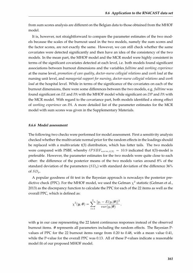
8.6 Application to the RN4CAST data set
from sum scores analysis are different on the Belgian data to those obtained from the MHOFmodel.
It is, however, not straightforward to compare the parameter estimates of the two mod-els because the scales of the burnout used in the two models, namely the sum scores andthe factor scores, are not exactly the same. However, we can still check whether the samecovariates were detected significantly and then have an idea of the consistency of the twomodels. In the mean part, the MHOF model and the MCR model were highly consistent interms of the significant covariates detected at each level, i.e. both models found significantassociations between burnout dimensions and the variables fulltime and working experienceat the nurse level, promotion of care quality, doctor-nurse collegial relations and work load at thenursing unit level, and managerial support for nursing, doctor-nurse collegial relations and workload at the hospital level. While in terms of the significance of the covariates on each of theburnout dimensions, there were some differences between the two models, e.g. fulltime wasfound significant on EE and PA with the MHOF model while significant on DP and PA withthe MCR model. With regard to the covariance part, both models identified a strong effectof working experience on PA. A more detailed list of the parameter estimates for the MCRmodel with sum scores was given in the Supplementary Materials.
8.6.6 Model assessment
The following two checks were performed for model assessment. First a sensitivity analysischecked whether the multivariate normal prior for the random effects in the loadings shouldbe replaced with a multivariate t(3) distribution, which has fatter tails. The two modelswere compared with PSBF, whereby `PSBFnorm,t(3) = 10.9 indicated that t(3)-model ispreferable. However, the parameter estimates for the two models were quite close to eachother: the difference of the posterior means of the two models varies around 8% of thestandard deviation of the parameters (SDp) with standard deviation of the difference 36%of SDp.
A popular goodness of fit test in the Bayesian approach is nowadays the posterior pre-dictive check (PPC). For the MHOF model, we used the Gelman χ2 statistic (Gelman et al.,2013) as the discrepancy function to calculate the PPC for each of the 22 items as well as theoverall PPC, which is defined as:
χ2(y, θ) =
n∑i=1
[yi − E(yi|θ)]2
var(yi|θ),
with y in our case representing the 22 latent continuous responses instead of the observedburnout items. θ represents all parameters including the random effects. The Bayesian P-values of PPC for the 22 burnout items range from 0.20 to 0.48, with a mean value 0.41,while the P-value for the overall PPC was 0.13. All of these P-values indicate a reasonablemodel fit of our proposed MHOF model.
161
Chapter 8 Multilevel Higher Order Factor Model
8.6.7 Clinical interpretation
The current study extends the theoretical and empirical knowledge of burnout measured bythe Maslach Burnout Inventory by examining both the mean and the covariance structureof the burnout dimensions in relation to work setting and individual factors, taking intoaccount the latent nature of the burnout dimensions and the multilevel research design.First, with regards to the latent nature of the burnout dimensions, our findings showed thatthe Maslach Burnout Inventory exhibited evidence of configural invariance. The problemsin factor loadings that we found with items 6 and 16 have previously been reported in ameta-analytic study of MBI factor analyses (Worley et al., 2008) and in a large multicoun-try nurse workforce study with a similar research design (Poghosyan et al., 2009). Second,our findings in both the mean and the variance parts of the three latent burnout dimen-sions have interesting clinical meanings. In the mean part, we found that both work set-ting and individual factors affected the burnout dimensions. Doctor-nurse collegial relationshad a complex relationship to the burnout dimensions. At the nursing unit level, betterrelations between doctors and nurses are related to less feelings of depersonalization andhigher rates of personal accomplishment. At the hospital level however, better relationswere related to higher degrees of emotional exhaustion. Such association has to our knowl-edge not been reported previously and needs close attention in further research. Findingsfor the other two work setting factors demonstrated that these operate differently at dif-ferent levels, with promotion of care quality and managerial support for nursing having effectsonly at the nursing unit level and hospital level respectively. Studies in which the relation-ship between work setting factors and outcomes are examined at multiple levels, have onlyemerged recently in the nursing literature (Li et al., 2013a,b; Gabriel et al., 2013). Previousresearch studies mostly showed findings that were likely to be very similar in terms of repli-cating the same relationships between aggregated work setting factors and outcomes, evenin different study settings. Studies such as this allow for more refined and more context-specific insights. Although in general the implications are similar, i.e. better work settingsresult in better outcomes, there is a larger degree of variation between the study findings.That is, in different settings, different work setting factors at different levels have a differentimpact on outcomes. As such, these studies demonstrate that policy makers and human re-sources managers in different settings need to implement different management strategiesto achieve better outcomes. In line with previously reported research findings, our findingsalso show that such management strategies should be very specific for nurses with differentwork experience and working status. Indeed, more experienced nurses tend to suffer lessfrom emotional exhaustion and depersonalization than less experienced nurses. Higher de-grees of job burnout among younger, less experienced workers have been reported beforeand can be the consequence of unsuccessful occupational socialization (Bakker et al., 2002).It could also be hypothesized that experienced nurses may have developed better copingmechanisms for burnout, or that workload and scope of practice are more fit to experiencednurses. Further, our results indicate that fulltime nurses suffer more from emotional exhaus-tion but have a higher sense of personal accomplishment, compared to part-time workingnurses. In line with our findings, Burke and Greenglass (2000), who measured the effects of
162
8.7 Conclusions
hospitals restructuring on 1362 nurses, found that full-time staff were more emotionally ex-hausted and depersonalized, yet reported greater professional efficacy. This evidence sup-ports the multidimensional measurement of burnout and opposes analytic strategies thatsolely focus on emotional exhaustion as the one and only hallmark of burnout (Schaufeliet al., 2009). It might also imply that caution is warranted in using SEM to model a causalpattern of relationships among the burnout dimensions (Bakker et al., 2002; Van Bogaertet al., 2013), in which emotional exhaustion has a direct impact on depersonalization and anindirect impact on reduced personal accomplishment. As shown here, personal accomplish-ment can develop independently of emotional exhaustion, which was previously theorizedby Leiter (1993). Already in the development of the MBI, Maslach and Jackson (1981) statedthat the personal accomplishment subscale is independent of the emotional exhaustion anddepersonalization subscales and cannot be assumed to be the opposite of these subscales.
The covariance part provides additional insights into the burnout phenomenon. Find-ings suggest a significantly larger variation in personal accomplishment for experiencednurses. A reason might be that, over the years, differences in nurses’ feelings related tointrinsic rewards (e.g. high collaboration with colleagues, positive patient experiences) andextrinsic rewards (e.g. salary, opportunities for advancement) become more pronounced.The fixed effects in the variance part reflect the temporal or demographical measurementof the variation of burnout. The justification of including random effects implies that thecovariances and the correlations among burnout are different across hospitals and nursingunits. A larger value indicates more heterogeneity of burnout feelings among nurses withina unit (a hospital or a nursing unit). We call this the measurement of ”harmonic burden”, i.e.the units with smaller variances reflect a better harmonic burden within it. Different fromthe fixed effects in the variance part, the random effects reflect the spatial or geographicalmeasurement of the variation of burnout.
8.7 Conclusions
Our proposed multilevel higher-order factor model provides a way to directly assess theheteroscedasticity of the multi-dimensional lower-order factor scores in a complex situa-tion. In a multi-center (-district, -country, etc.) study where the interested measurementmight not be observed directly but is a latent construct obtained from a factor analyticmodel, a traditional structural equation modeling approach could be applied. The latentconstruct might however show heteroscedasticity because of e.g. the ”cultural difference”among centers, districts, countries, etc., or because of different characteristics of the individ-uals. We then strongly recommend researchers to apply the proposed MHOF model thatcould efficiently combine the factor analytic model and a regression model, while takinginto account the multilevel structure as well as the heteroscedasticity. This modeling canreveal some ”hidden” information that may have never been obtained through modelingonly the mean of the measurements. For example, the larger variance/covariance matrix insome nursing unit in our motivating data set may imply the unbalanced burden of nursingcare within that nursing unit. Therefore this could provide valuable information for the ad-
163
Chapter 8 Multilevel Higher Order Factor Model
ministration of the hospitals and nursing units. The contribution of this paper is howevernot confined to nursing research. Our methods apply equally well to numerous researchtopics in psychology, sociology and political science, to name a few, which often deal withmultilevel research designs, latent constructs, and an interest in covariance regression.
References
Asparouhov, T. and Muthen, B. (2005). Multivariate statistical modeling with survey data.In Paper Presented at the Federal Committee on Statistical Methodology (FCSM) Research Confer-ence.
Asparouhov, T. and Muthen, B. (2009). Exploratory structural equation modeling. Struc-tural Equation Modeling: A Multidisciplinary Journal, 16(3):397–438.
Bakker, A. B., Demerouti, E., and Schaufeli, W. B. (2002). Validation of the maslach burnoutinventory-general survey: An internet study. Anxiety, Stress & Coping, 15(3):245–260.
Brooks, S. and Gelman, A. (1998). General methods for monitoring convergence of iterativesimulations. Journal of Computational and Graphical Statistics, 7(4):434–455.
Burke, R. J. and Greenglass, E. R. (2000). Effects of hospital restructuring on full time andpart time nursing staff in Ontario. International Journal of Nursing Studies, 37(2):163–171.
Burton, A., Altman, D. G., Royston, P., and Holder, R. L. (2006). The design of simulationstudies in medical statistics. Statistics in Medicine, 25(24):4279–4292.
Collins, L., Schafer, J., and Kam, C. (2001). A comparison of inclusive and restrictive strate-gies in modern missing data procedures. Psychological Methods, 6(4):330–351.
DiStefano, C., Zhu, M., and Mindrila, D. (2009). Understanding and using factor scores:Considerations for the applied researcher. Practical Assessment, Research & Evaluation,14(20):1–11.
Gabriel, A. S., Erickson, R. J., Moran, C. M., Diefendorff, J. M., and Bromley, G. E. (2013).A multilevel analysis of the effects of the practice environment scale of the nursing workindex on nurse outcomes. Research in Nursing & Health, 36(6):567–581.
Gelman, A., Carlin, J. B., Stern, H. S., Dunson, D. B., Vehtari, A., and Rubin, D. B. (2013).Bayesian Data Analysis. Chapman and Hall/CRC, 3rd edition.
Goldstein, H. (2010). Multilevel Statistical Models (Wiley Series in Probability and Statistics).Wiley, 4th edition.
Hoff, P. and Niu, X. (2012). A covariance regression model. Statistica Sinica, 22(2):729–753.
Hox, J. (2010). Multilevel Analysis: Techniques and Applications (Quantitative MethodologySeries). Routledge, 2nd edition.
Hu, L.-t. and Bentler, P. M. (1999). Cutoff criteria for fit indexes in covariance structureanalysis: Conventional criteria versus new alternatives. Structural Equation Modeling: AMultidisciplinary Journal, 6(1):1–55.
Ibrahim, J. G., Chen, M.-H., and Lipsitz, S. R. (2002). Bayesian methods for generalizedlinear models with covariates missing at random. Canadian Journal of Statistics, 30(1):55–78.
Joreskog, K. G. and Goldberger, A. S. (1975). Estimation of a model with multiple indicatorsand multiple causes of a single latent variable. Journal of the American Statistical Association,70(351a):631–639.
Kline, R. B. (2010). Principles and Practice of Structural Equation Modeling (Methodology in theSocial Sciences). The Guilford Press, 3rd edition.
164
References
Kutney-Lee, A., McHugh, M., Sloane, D., Cimiotti, J., Flynn, L., Neff, D., and Aiken, L.(2009). Nursing: a key to patient satisfaction. Health Affairs, 28(4):w669–w677.
Leiter, M. P. (1993). Burnout as a developmental process: Consideration of models. InSchaufeli, W. B., Maslach, C., and Marek, T., editors, Professional burnout: Recent develop-ments in theory and research. Series in applied psychology: Social issues and questions, pages237–250. Philadelphia, PA, US: Taylor & Francis.
Lesaffre, E. and Lawson, A. B. (2012). Bayesian Biostatistics (Statistics in Practice). Wiley, 1stedition.
Lesaffre, E., Rizopoulos, D., and Tsonaka, R. (2007). The logistic transform for boundedoutcome scores. Biostatistics, 8(1):72–85.
Li, B., Bruyneel, L., and Lesaffre, E. (2013a). A multivariate multilevel Gaussian modelwith a mixed effeccts structure in the mean and covariance part. Statistics in Medicine.(accepted).
Li, B., Bruyneel, L., Sermeus, W., Van den Heede, K., Matawie, K., Aiken, L., and Lesaffre,E. (2013b). Group-level impact of work environment dimensions on burnout experiencesamong nurses: A multivariate multilevel probit model. International Journal of NursingStudies, 50(2):281–291.
Longford, N. and Muthen, B. (1992). Factor analysis for clustered observations. Psychome-trika, 57(4):581–597.
Maruyama, G. M. (1997). Basics of Structural Equation Modeling. SAGE Publications, Inc, 1stedition.
Maslach, C. and Jackson, S. E. (1981). The measurement of experienced burnout. Journal ofOrganizational Behavior, 2(2):99–113.
Maslach, C., Jackson, S. E., and Leiter, M. P. (1996). Maslach Burnout Inventory Manual, 3rdedition.
Muthen, B. and Asparouhov, T. (2012). Bayesian structural equation modeling: A moreflexible representation of substantive theory. Psychological Methods, 17(3):313–335.
Muthen, B. O. (1994). Multilevel covariance structure analysis. Sociological Methods & Re-search, 22(3):376–398.
Muthen, L. and Muthen, B. (2010). Mplus User’s guide. Los Angeles: Muthen & Muthen,6th edition.
Neuhaus, J. M. and Kalbfleisch, J. D. (1998). Between- and within-cluster covariate effectsin the analysis of clustered data. Biometrics, 54(2):638–645.
Plummer, M. (2003). JAGS: A program for analysis of Bayesian graphical models usingGibbs sampling. In The 3rd International Workshop on Distributed Statistical Computing (DSC2003). March.
Plummer, M. (2013). Package rjags version 3-10.
Poghosyan, L., Aiken, L. H., and Sloane, D. M. (2009). Factor structure of the Maslachburnout inventory: an analysis of data from large scale cross-sectional surveys of nursesfrom eight countries. International Journal of Nursing Studies, 46(7):894–902.
Schaufeli, W. B., Enzmann, D., and Girault, N. (1993). Measurement of burnout: A re-view. In Schaufeli, W. B., Maslach, C., and Marek, T., editors, Professional burnout: Recentdevelopments in theory and research, pages 199–215. Washington, DC: Taylor & Francis.
Schaufeli, W. B., Leiter, M. P., and Maslach, C. (2009). Burnout: 35 years of research andpractice. Career Development International, 14(3):204–220.
165

Chapter 8 Multilevel Higher Order Factor Model
Sermeus, W., Aiken, L., Van den Heede, K., Rafferty, A., Griffiths, P., Moreno-Casbas, M.,Busse, R., Lindqvist, R., Scott, A., Bruyneel, L., et al. (2011). Nurse forecasting in Europe(RN4CAST): Rationale, design and methodology. BMC Nursing, 10(1):6.
Smith, H. L. (2008). A double sample to minimize skew due to non-response in a mailsurvey. In Ruiz-Gazen, A., Guilbert, P., Haziza, D., and Tille, Y., editors, Survey methods:Applications to longitudinal investigations, health, electoral investigations, and investigations inthe developing countries, pages 334–339. Paris: Dunod.
Spiegelhalter, D., Best, N., Carlin, B., and Van Der Linde, A. (2002). Bayesian measures ofmodel complexity and fit. Journal of the Royal Statistical Society: Series B (Statistical Method-ology), 64(4):583–639.
Steenkamp, J.-B. E. and Baumgartner, H. (1998). Assessing measurement invariance incross-national consumer research. Journal of Consumer Research, 25(1):78–107.
Van Bogaert, P., Kowalski, C., Weeks, S. M., Clarke, S. P., et al. (2013). The relationship be-tween nurse practice environment, nurse work characteristics, burnout and job outcomeand quality of nursing care: A cross-sectional survey. International Journal of Nursing Stud-ies, 50(12):1667–1677.
Worley, J. A., Vassar, M., Wheeler, D. L., and Barnes, L. L. (2008). Factor structure of scoresfrom the Maslach burnout inventory: A review and meta-analysis of 45 exploratory andconfirmatory factor-analytic studies. Educational and Psychological Measurement, 68(5):797–823.
166

9CONCLUSIONS
167

9.1 General conclusions
9.1 General conclusions
A traditional multilevel regression model assumes a constant residual variance after adjust-ing for the fixed and random effects. The focus of this modeling approach is on the expectedvalue (the mean) of the response that can vary with covariates (e.g. age) and across the levelof the units (e.g. medical centers in a multi-center study). When heteroscedasticity exists inthe multilevel context also, the variance may depend on covariates and on random effects,resulting in a mixed effects regression model for the variance with an expression similar asfor a mixed effects regression model of the mean. In the multivariate case, not only the vari-ances, but also the covariance(s) or the correlation(s), can be regressed on fixed and randomeffects. The proposed models in this thesis handle this complex situation well. We calledthis modeling approach multilevel covariance regression (MCR). Modeling of the covari-ance matrix in our MCR model is done by implementing a factor analytic (FA) model to theresidual part of a multivariate random effects model. The Bayesian approach is chosen asthe preferred estimating method because of its flexibility in handling complex situations.
The MCR model aims at modeling heteroscedasticity with both fixed and random effectsin a multivariate and multilevel situation. This provides a way of obtaining insight in thefactors that determine the level of the response and their variability. The multidimensionalconstruct of work-related nurse burnout, measured in the multi-country Registered NurseForecasting (RN4CAST) study, provides an excellent example of how our innovative sta-tistical model provides new substantive insights. This is illustrated in Chapters 6, 7 and 8.With the classical multilevel regression model we demonstrated that nurses’ working experi-ence has a negative effect on the mean burnout measures (i.e. more experienced nurses tendto be less burnout), while with the multilevel covariance regression model we showed inaddition that the variation of burnout depends on nurses’ working experience and randomeffects at each level. The variance of the random effects in the variance part may indicatethe extend to which there is inequality of nursing care activity within a given unit (whichwe refer to as ”harmonic burden” in Chapter 8). Therefore it can give valuable suggestionsto the management of nursing care within a country, hospital or nursing unit.
The type of the response of the multilevel covariance regression model could be binary(Chapter 6), continuous but possibly with a non-standard distribution (e.g. bounded out-come scores in Chapter 7), ordinal, etc., or a combination of these types. Further, if theresponse comes from another model, it is also possible to jointly estimate the two models.In Chapter 8, the burnout response of the multilevel covariance regression model is a re-sult from the factor scores in a multilevel factor analytic (MFA) model, and estimation fromsimultaneously fitting two models (MFA and MCR models) yields a multilevel higher or-der factor (MHOF) model. An advantage of this model is that the original items from thequestionnaire are used instead of predefined dimensions. This, together with modeling theheteroscedasticity, provides some clues on the differences between the factor structure ofthe current data set and that of the predefined structure.
To conclude, the multilevel covariance regression model with different types of responseperformed well when applied to the RN4CAST data set using the Bayesian approach. With
169
Chapter 9 Conclusions
regard to nursing research, our model provides more refined analyses of the relationshipsbetween nurses’ burnout and their characteristics as well as the organizational-level covari-ates. Findings allow insights not only for the mean measures of burnout, but also for thecorrelations among the three burnout dimensions. The proposed model thus uses the datamore efficiently. Not confined to nursing research only, our proposed modeling approachesapply equally well to many other research fields with multilevel research designs, latentconstructs, and where there is an interest in covariance regression.
9.2 Future research
In this section we suggest topics for future research on the multilevel covariance regressionmodel. Specifically, we will discuss further extensions of the MCR and MHOF models, aswell as Bayesian model assessment.
9.2.1 Model extension
The MHOF model combines the MCR model with a multilevel factor analytic (MFA) model,whereby the nurse-level factor scores from the MFA model are used as the burnout re-sponses in the MCR model. Similarly, we could also use the factor scores for the covariatework environment which is measured through a 32-item questionnaire. Namely, we could fitan MFA model for work environment, and extract the factor scores at each level to replacethe used work environment variables in the MHOF model. These work environment variableswere generated from a predefined factor structure based on a different population. Thecombination implies a simultaneous estimation of the MHOF and the MFA models. Thecomputation, however, might be quite demanding as more random effects and latent vari-ables are modeled.
So far, only the nurse-level covariance matrix of the three burnout dimensions is consid-ered depending on fixed and random effects. It is also possible to model the higher-level co-variance matrices of the MCR and MHOF models with both fixed and random effects. Thisextension can address the following question, e.g. ”do the nursing unit-level correlationsof burnout remain constant across hospitals and across the characteristics of the nursingunit?”.
9.2.2 Bayesian model assessment
We first discuss the selection of the number of latent factors in a FA model. As the firstexploratory step of an MHOF model, a multilevel exploratory factor analytic model wasconducted in Chapter 8 to find the factor structure of burnout. For this, the frequentistapproach using the program Mplus produces many approximate indices to evaluate the fitof a FA model, such as RMSEA, TLI, CLI, SRMR, etc. These can help us determine thenumber of latent factors for a parsimonious FA model with a reasonable model fit. In aBayesian context, the number of factors can be determined by comparing the goodness-of-fit indices, e.g. the posterior predictive checks with an appropriate discrepancy measure. Amore formal method was proposed by Lopes and West (2004) who utilized the reversible
170
References
jump MCMC method for this purpose. Either way needs closer investigation to evaluate itsperformance on our proposed models.
The Bayesian model comparison for our proposed MCR and MHOF models can be quitechallenging especially when the response is not of standard form, such as the BOS typeof response (bounded outcome scores) used in Chapters 7 and 8. Both for DIC and PSBF(pseudo Bayes factor) we encountered difficulties with the multivariate BOS response. ForPSBF, it would be of interest in general, how to incorporate model complexity and to applyand test this on the MCR and MHOF models.
References
Lopes, H. F. and West, M. (2004). Bayesian model assessment in factor analysis. StatisticaSinica, 14(1):41–68.
171
Summary
The multilevel model is the focus for all chapters in this thesis. We have compared softwarefor handling one type of this model, namely the logistic random effects regression model.The multilevel factor analytic (MFA) model and multilevel structural equation modeling(multilevel SEM) are also applied. Inspired by a number of clinical research questions fromthe Registered Nurse Forecasting (RN4CAST) study, we have further developed two novelmodeling approaches based on the multilevel model to handle more complex situations.These are the multilevel covariance regression (MCR) modeling and the multilevel higher-order factor (MHOF) modeling.
Chapter 3 compares the commonly used packages/programmes for handling several lo-gistic random effects regression models. Both frequentist and Bayesian approaches werereviewed. Frequentist approaches included R (lme4), Stata (GLLAMM), SAS (GLIMMIXand NLMIXED), MLwiN ([R]IGLS) and MIXOR; Bayesian approaches included WinBUGS,MLwiN (MCMC), R package MCMCglmm and SAS experimental procedure MCMC. Wesaw that most often the packages gave similar parameter estimates, but they differ consider-ably in flexibility, computation time and usability. The frequentist and Bayesian approachesalso performed differently for the small sample problem. The Bayesian approach, thoughsometimes time-consuming, showed the greatest flexibility in modeling.
In Chapters 4 to 8, the RN4CAST data set, collected in the context of a large Europeannurse survey project, was the main inspiration for new statistical developments. In Chapter4, a logistic random effects model was applied to a list of nursing tasks below their skilllevel they performed during the daily nursing work. It allowed for a comparison betweentasks performed by domestically trained nurses and foreign trained nurses from developingcountries.
In Chapter 5, the focus is on the nursing work environment rated by each nurse. A two-level multiple indicators multiple causes (MIMIC) model was applied to detect differencesbetween nursing unit managers’ and staff nurses’ opinions on the work environment. Wefound out that for certain work environment dimensions, nursing unit managers had morepositive opinions compared to nurses.
In Chapters 6 to 8 the burnout measurement of the nurses was of interest. As the orig-inal measure of burnout was not normally distributed, a dichotomized burnout variablewas used in Chapter 6. The relationship between burnout and the work environmentwas examined in a four-level context while taking into account the intra-class correlationand heteroscedasticity of the binary burnout measurement. Modeling of heteroscedasticitywas achieved through a built-in factor analytic model wherein the factor loadings changedacross units (countries, hospitals and nursing units). This is actually a first step and a simpleversion of the multilevel covariance regression model proposed in Chapter 7.
As an extension of the model in Chapter 6, we proposed the multilevel covariance re-gression (MCR) model in Chapter 7. This model can handle the original non-normallydistributed burnout measures as well as modeling the heteroscedasticity with both fixedand random effects. The properties of the MCR model, the identification issues and the
172
Summary
interpretations were carefully described in detail. The simulation study showed good per-formance of the model in handling outliers at each level. The application to the data fromthe RN4CAST study revealed new insights that could not be found through classic mixedmodels.
A further extension of the MCR model was described in Chapter 8, which is called themultilevel higher order factor (MHOF) model. It replaces the response in the MCR modelwith the factor scores coming from a multilevel factor analytic model, which was estimatedsimultaneously with the MCR model. This brought in more challenges on e.g. computation,identification, etc. Our proposed Bayesian method could handle this complex situation well.
173
Samenvatting
In deze thesis hebben we het hierarchisch model toegepast op verpleegkundige gegevensen uitbreidingen voorgesteld voor het multivariate respons geval. In de eerste twee hoofd-stukken hebben we de basisconcepten ingeleid nodig voor deze thesis.
Hoofdstuk 3 vergelijkt de populaire software voor de verschillende logistisch randomeffects regressie modellen; zowel frequentistische als Bayesiaanse benaderingen werden be-handeld. De frequentistische software was: R (lme4), Stata (GLLAMM), SAS (GLIMMIX enNLMIXED), MLwiN ([R]IGLS) en MIXOR en de Bayesiaanse software was: WinBUGS, ML-wiN (MCMC), R pakket MCMCglmm en de toen experimentele SAS (versie 9.2) procedureMCMC. Onze vergelijking liet zien dat vaak de meeste pakketten similaire parameter schat-tingen gaven, maar ook dat ze aardig konden verschillen in flexibiliteit, berekeningstijden gebruiksvriendelijkheid. De performantie van de frequentistische en de Bayesiaansemethodes verschilden ook voor kleine steekproeven. De Bayesiaanse aanpak, weliswaarvaak meer computerintensief, vertoonde de grootste flexibiliteit in het modelleren van degegevens.
In hoofdstukken 4 tot 8 hebben we de RN4CAST data set intensief gebruikt. Deze dataset was het resultaat van een grootschalig Europees project dat werd opgezet om meerinzicht te bekomen in de relatie werkomgeving en werkervaring bij verpleegkundigen. Inhoofdstuk 4 hebben we een logistisch random effect model gebruikt om de factoren te on-derzoeken die bepalen waarom verpleegkundigen taken uitvoerden die niet tot hun oor-spronkelijk takenpakket hoorden en beneden hun competentie lagen. Het model vergelijkthierin ook de verpleegkundigen opgeleid in de respectievelijke RN4CAST landen met deverpleegkundigen opgeleid in hun ontwikkelingsland van herkomst.
In hoofdstuk 5, hebben we de verpleegkundige werkomgeving, zoals gescoord door deverpleegkundigen in de RN4CAST studie, onderzocht. We hebben hiervoor een hierar-chisch model met twee niveaus en meerdere indicatoren (MIMIC model) toegepast om deverschillende beleving van de werkomgeving te bestuderen tussen de hoofden van de ver-pleegkundige afdelingen enerzijds en de verpleegkundigen in die respectievelijke afdelin-gen anderzijds. Onze analyse wees uit dat voor bepaalde werkomgevingsvariabelen dehoofden een duidelijk meer rooskleurig beeld hadden dan de verpleegkundigen zelf.
In hoofstukken 6 tot 8 hebben we burnout bij verpleegkundigen onderzocht. Omdatde originele burnout maat niet normal verdeeld is, hebben we deze gedichomotomiseerdin hoofdstuk 6. We hebben dan de relatie tussen deze binaire burnoutmaat en de ver-pleegkundige werkomgeving onderzocht in een hierarchisch model met 4 niveau’s reken-ing houdende met de heteroscedasticiteit van de binaire burnout metingen. We hebbende heteroscedasticiteit gemodelleerd met behulp van een factor analytische aanpak waar-bij de factorladingen mogen verschillen tussen de verpleegeenheden (landen, hospitalenen verpleegeenheden). Dit was de eerste stap en een eenvoudige versie van hierarchischcovariantie regressie model voorgesteld het volgende hoofdstuk.
In hoofdstuk 7 hebben we het voorgaande model uitgebreid tot het hierarchisch co-variantie regressie (MCR) model. Dit model werkt op de originele niet-normaalverdeelde
174
Samenvatting
burnoutmaten en modelleert de heteroscedasticiteit als een mixed effects model. In dithoofdstuk hebben we ook de eigenschappen van het MCR model onderzocht, alsook de in-terpretatie van de modelparameters en de mogelijke identificatieproblemen voor het bepalenvan parameterschattingen. Een simulatiestudie toonde aan dat het model geschikt is om devariabiliteit van de variantie-covariantie matrix aan het licht te brengen. Toegepast op deRN4CAST studie, bleek uit het MCR model ook de invloed van werkomgeving op de vari-abiliteit van de burnoutmaten.
In hoofdstuk 8 stellen we een uitbreiding van het MCR model voor, genaamd het hier-archisch hogere orde factor (MHOF) model. Dit vervangt de hoog-dimensionele responsin het MCR model door de factor scores uit een hierarchisch factor analytisch model. Deparameters van de twee deelmodellen (MFA en MCR) worden gezamenlijk geschat. Ditbracht extra uitdagingen met zich mee, zoals bijvoorbeeld bijkomende computationele enidentificatie problemen. Echter, de Bayesiaanse aanpak leverde geen problemen op voordeze verdere uitbreiding.
175

Acknowledgements
This journey has finally come to an end for the moment. It is a pleasant journey, althoughit is never easy. I am quite amazed by what I’ve done so far when looking at the thesis infront of me, indeed. It would not have been possible to finish this without all kinds of helparound me. I am very grateful to all my colleagues, my friends and my family.
First and foremost I would like to thank my supervisor Emmanuel Lesaffre who has beensupporting me enormously with great patient and with brilliant ideas. And also thank youfor guiding me into the beautiful new world of Bayesian. I feel so proud of being in thisfield.
I would also like to give my sincere thanks to all my colleagues from the Biostatisticsdepartment in EMC. Being a member of this international family is the fortune of my wholelife. I would like to thank Eline, Siti, Karolina, Johan, Paul, Sten, Magdalena, Dimitris,Vironika, Susan, Elrozy, Kazem, Joost, Nicole, Betina, Maria, Lidia, Wim, Gianluca, Sara,Els, Dymph, Cibele, Anne, Kees, Ehsan, Benedict and also some new members of the family.Thank you all for creating such great atmosphere. I would like to give my special thanks toa former colleague Marek who helped me kindly whenever I had problems for my project.May you rest in peace in heaven.
I also owe my thanks to a lot of friends outside my department. I would like to thankProf. Steyerberg, Hester, Rachel, Nano, Astrid and Adi from this university, and I wouldlike to thank Luk, Prof. Sermeus, and Luwis from the university of Leuven for the long termpleasant and successful collaboration. I would like to thank Bonnie and Chang. Chang, youare one of the friends I knew for the longest time here and you are always so kind andwilling to help.
时间过得很快,4 年多的博士生涯马上结束了。一个人漂泊在海外的生活并不容易, 所幸结识了
一帮志同道合的朋友及损友,让生活变得不乏味。在这里大家一同留下了太多值得纪念的回忆。
大怪路子,杀人游戏,K 歌,大大小小的聚餐,BBQ,乒乓,羽毛球,踢毽子,桌球,滑雪,钓鱼,
挖生蚝,等等。在此,我要感谢我的朋友海波,稚超,徐洪,路狄非,康宁,刘凡,温蓓,孙伟,
海燕,程姐,吕鹏,甜娜,睽睽,天石,蔡蕊,明慧,小娜夫妇,吴庆夫妇,艳楠夫妇,舟桥夫
妇,商鹏夫妇,胡晗,凯音,展民,莹颖,田田,玺峰,黄龄,刘哲,朱玉,唐晖,亚迪,克若,
栾莹,延伟, 亚楠,等等,感谢你们让我在这里度过了难忘的时光。
At last, I would like to thank my parents and my two elder sisters, for their selfless sup-port all along the way. I owe my sincere thanks to my wife for being so persistent andapprehensive and for supporting me in all aspects.
176
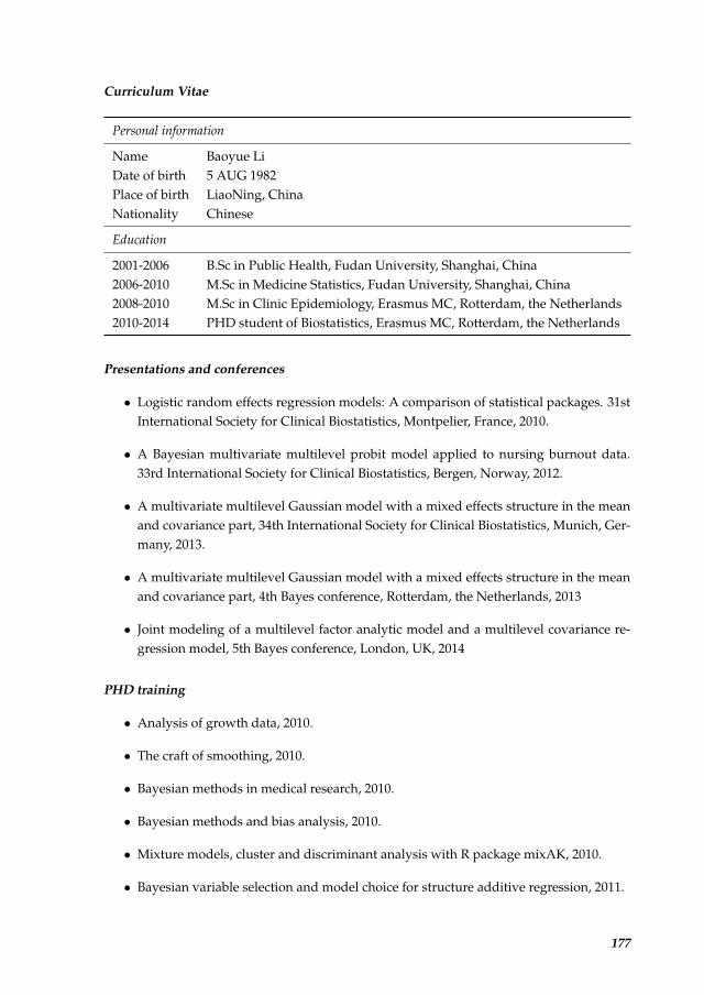
Curriculum Vitae
Personal information
Name Baoyue LiDate of birth 5 AUG 1982Place of birth LiaoNing, ChinaNationality Chinese
Education
2001-2006 B.Sc in Public Health, Fudan University, Shanghai, China2006-2010 M.Sc in Medicine Statistics, Fudan University, Shanghai, China2008-2010 M.Sc in Clinic Epidemiology, Erasmus MC, Rotterdam, the Netherlands2010-2014 PHD student of Biostatistics, Erasmus MC, Rotterdam, the Netherlands
Presentations and conferences
• Logistic random effects regression models: A comparison of statistical packages. 31stInternational Society for Clinical Biostatistics, Montpelier, France, 2010.
• A Bayesian multivariate multilevel probit model applied to nursing burnout data.33rd International Society for Clinical Biostatistics, Bergen, Norway, 2012.
• A multivariate multilevel Gaussian model with a mixed effects structure in the meanand covariance part, 34th International Society for Clinical Biostatistics, Munich, Ger-many, 2013.
• A multivariate multilevel Gaussian model with a mixed effects structure in the meanand covariance part, 4th Bayes conference, Rotterdam, the Netherlands, 2013
• Joint modeling of a multilevel factor analytic model and a multilevel covariance re-gression model, 5th Bayes conference, London, UK, 2014
PHD training
• Analysis of growth data, 2010.
• The craft of smoothing, 2010.
• Bayesian methods in medical research, 2010.
• Bayesian methods and bias analysis, 2010.
• Mixture models, cluster and discriminant analysis with R package mixAK, 2010.
• Bayesian variable selection and model choice for structure additive regression, 2011.
177

• Missing Data in Longitudinal Studies: Strategies for Bayesian Modeling, SensitivityAnalysis, and Causal Inference, 2011.
• New Features Mplus version 7, 2012.
• Bayesian variable selection, 2012.
• Bayesian adaptive methods for clinical trials, 2012.
• An introduction to the joint modeling of longitudinal and survival data, 2013.
Assistant teaching
• Bayesian methods, Nihes, 2012-2014.
• Modern methods, Nihes, 2011-2013.
• Classical methods, Nihes, 2010-2013.
• Repeated measurement, Nihes, 2012-2014.
• Multiple regression methods using SPSS, 2011-2014.
• Introduction to epidemiology, Nihes summer programme, 2011-2012.
178
Publications
Li, B., Bruyneel, L., and Lesaffre, E. (2014). Multilevel higher-order factor model: Joint mod-eling of a multilevel factor analytic model and a multilevel covariance regression model.Structural Equation Modeling: A Multidisciplinary Journal. (under review)
Bruyneel, L., Li, B., Squires, A., Gilmartin, M., Spotbeen, S., Meuleman, B., Lesaffre, E., andSermeus, W. (2014). Nursing unit managers’ and staff nurses’ opinions of the nursing workenvironment: a Bayesian multilevel mimic model for cross-group comparisons. Research inNursing & Health (under review)
Diya, L., Li, B., Heede, K., Sermeus, W., and Lesaffre, E. (2014). Multilevel factor analyticmodels for assessing the relationship between nurse’ reported adverse events and patientsafety. Journal of the Royal Statistical Society: Series A (Statistics in Society), 177(1):237-257.
Li, B., Bruyneel, L., and Lesaffre, E. (2014). A multivariate multilevel Gaussian model witha mixed effects structure in the mean and covariance part. Statistics in Medicine, 33(11):1877-1899.
Bruyneel, L., Li, B., Squires, A., Aiken, L., Lesaffre, E., Van den Heede, K., and Sermeus,W. (2013). A multi-country perspective on nurses tasks below their skill level: Reportsfrom domestically trained nurses and foreign trained nurses from developing countries.International Journal of Nursing Studies, 50(2):202-209.
Croughs, P. D., Li, B., Hoogkamp-Korstanje, J. A. A., and Stobberingh, E. (2013). Thirteenyears of antibiotic susceptibility surveillance of Pseudomonas aeruginosa from intensivecare units and urology services in the Netherlands. European Journal of Clinical Microbiology& Infectious Diseases, 32(2):283-288.
Schubert, M., Ausserhofer, D., Desmedt, M., Schwendimann, R., Lesaffre, E., Li, B., and DeGeest, S. (2013). Levels and correlates of implicit rationing of nursing care in Swiss acutecare hospitals: A cross sectional study. International Journal of Nursing Studies, 50(2):230-239.
Li, B., Bruyneel, L., Sermeus, W., Van den Heede, K., Matawie, K., Aiken, L., and Lesaf-fre, E. (2013). Group-level impact of work environment dimensions on burnout experiencesamong nurses: A multivariate multilevel probit model. International Journal of Nursing Stud-ies, 50(2):281-91.
Li, B., Lingsma, H. F., Steyerberg, E. W., and Lesaffre, E. (2011). Logistic random effectsregression models: A comparison of statistical packages for binary and ordinal outcomes.BMC Medical Research Methodology, 11(1):77.
Lingsma, H. F., Roozenbeek, B., Li, B., Lu, J., Weir, J., Butcher, I., Marmarou, A., Murray, G.D., Maas, A. I., Steyerberg, E. W. (2011). Large between-center differences in outcome aftermoderate and severe traumatic brain injury in the international mission on prognosis andclinical trial design in traumatic brain injury (IMPACT) study. Neurosurgery, 68(3):601-608.
179