multilevel monte carlo for exponential levy models´ · multilevel monte carlo for exponential levy...

Noname manuscript No.(will be inserted by the editor)

Multilevel Monte Carlo For Exponential Levy Models

Michael B. Giles · Yuan Xia

Received: date / Accepted: date

Abstract We apply the multilevel Monte Carlo method for option pricing problemsusing exponential Levy models with a uniform timestep discretisation. For lookbackand barrier options, we derive estimates of the convergence rate of the error intro-duced by the discrete monitoring of the running supremum of a broad class of Levyprocesses. We then use these to obtain upper bounds on the multilevel Monte Carlovariance convergence rate for the Variance Gamma, NIG and α-stable processes. Wealso provide analysis of a trapezoidal approximation for Asian options. Our methodis illustrated by numerical experiments.

Keywords multilevel Monte Carlo · exponential Levy models · Asian options ·lookback options · barrier options

Mathematics Subject Classification (2000) MSC 65C05 ·MSC 91G60

1 Introduction

Exponential Levy models are based on the assumption that asset returns follow aLevy process [25,10]. The asset price follows

St = S0 exp(Xt) (1.1)

where Xt is an (m,σ ,ν)-Levy process

Xt = mt +σBt +∫ t

0

∫|z|≥1

z J(dz,ds)+∫ t

0

∫|z|<1

z(J(dz,ds)−ν(dz)ds)

Mike GilesMathematical Institute and Oxford-Man Institute of Quantitative Finance, Oxford UniversityE-mail: [email protected]

Yuan XiaMathematical Institute and Oxford-Man Institute of Quantitative Finance, Oxford UniversityE-mail: [email protected]

2 Michael B. Giles, Yuan Xia

where m is a constant, Bt is a Brownian Motion, J is the jump measure and ν is theLevy measure [24].

Models with jumps give an intuitive explanation of implied volatility skew andsmile in the index option market and foreign exchange market [10]. The jump fearis mainly on the downside in the equity market which produces a premium for low-strike options; the jump risk is symmetric in the foreign exchange market so theimplied volatility has a smile shape. [10] shows that models building on pure jumpprocesses can reproduce the stylized facts of asset returns, like heavy tails and theasymmetric distribution of increments. Since pure jump processes of finite activitywithout a diffusion component cannot generate a realistic path, it is natural to allowthe jump activity to be infinite. In this work we deal with infinite-activity pure jumpexponential Levy models, in particular models driven by Variance Gamma (VG),Normal Inverse Gaussian (NIG) and α-stable processes which allow direct simulationof increments.

We are interested in estimating the expected payoff value E[ f (S)] in option pric-ing problems. In the case of European options, it is possible to directly sample thefinal value of the underlying Levy process, but in the case of Asian, lookback andbarrier options the option value depends on functionals of the Levy process and soit is necessary to approximate those. In the case of a VG model with a lookback op-tion, the convergence results in [13] show that to achieve an O(ε) root mean square(RMS) error using a standard Monte Carlo method with a uniform timestep discretisa-tion requires O(ε−2) paths, each with O(ε−1) timesteps, leading to a computationalcomplexity of O(ε−3).

In the case of simple Brownian diffusion, Giles [16,17] introduced a multilevelMonte Carlo (MLMC) method, reducing the computational complexity from O(ε−3)to O(ε−2) for a variety of payoffs. The objective of this paper is to investigate whethersimilar benefits can be obtained for exponential Levy processes.

Various researchers have investigated simulation methods for the running maxi-mum of Levy processes. Reference [15] develops an adaptive Monte Carlo methodfor functionals of killed Levy processes with a controlled bias. Small-time asymptoticexpansions of the exit probability are given with computable error bounds. For evalu-ating the exit probability when the barrier is close to the starting point of the process,this algorithm outperforms a uniform discretisation significantly. Reference [20] de-velops a novel Wiener-Hopf Monte-Carlo method to generate the joint distribution of(XT ,sup0≤t≤T Xt

)which is further extended to MLMC in [14], obtaining an RMS er-

ror ε with a computational complexity of O(ε−3)

for Levy processes with boundedvariation and O

(ε−4)

for processes with infinite variation. The method currentlycannot be directly applied to VG, NIG and α−stable processes. References [12,11]adapt MLMC to Levy-driven SDEs with payoffs which are Lipschitz w.r.t. the supre-mum norm. If the Levy process does not incorporate a Brownian process, reference[11] obtains an O

(ε−(6β )/(4−β )

)upper bound on the worst case computational com-

plexity, where β is the BG index which will be defined later.In contrast to those advanced techniques, we take the discretely monitored maxi-

mum based on a uniform timestep discretisation of the Levy process as the approxi-mation. The outline of the work is as follows. First we review the Multilevel Monte

Multilevel Monte Carlo For Exponential Levy Models 3

Carlo method and present the three Levy processes we will consider in our numericalexperiments. To prepare for the analysis of the multilevel variance of lookback andbarrier, we bound the convergence rate of the discretely monitored running maximumfor a large class of Levy processes whose Levy measures have a power law behaviorfor small jumps, and have exponential tails. Based on this, we conclude by boundingthe variance of the multilevel estimators. Numerical results are then presented for themultilevel Monte Carlo applied to Asian, lookback and barrier options using the threedifferent exponential Levy models.

2 Multilevel Monte Carlo (MLMC) method

For a path-dependent payoff P based on an exponential Levy model on the timeinterval [0,T ], let P denote its approximation using a discretisation with M` uniformtimesteps of size h` = M−` T on level `; in the numerical results reported later, weuse M = 2. Due to the linearity of the expectation operator, we have the followingidentity:

E[PL] = E[P0]+L

∑`=1

E[P −P −1]. (2.1)

Let Y0 denote the standard Monte Carlo estimate for E[P0] using N0 paths, and for` > 0, we use N` independent paths to estimate E[P −P −1] using

Y` = N−1`

N`

∑i=1

(P(i)` −P(i)

`−1

). (2.2)

For a given path generated for P(i)` , we can calculate P(i)

`−1 using the same underlyingLevy path. The multilevel method exploits the fact that V` := V[P −P −1] decreaseswith `, and adaptively chooses N` to minimise the computational cost to achieve adesired RMS error. This is summarized in the following theorem in [18,19]:

Theorem 2.1 Let P denote a functional of St , and let P denote the correspondingapproximation using a discretisation with uniform timestep h` = M−` T . If there existindependent estimators Y` based on N` Monte Carlo samples, each with complexityC`, and positive constants α,β ,c1,c2,c3 such that α≥ 1

2 min(1,β ) and

i)∣∣∣E[P −P]

∣∣∣≤ c1 hα`

ii) E[Y`] =

{E[P0], `= 0

E[P − P −1], ` > 0

iii) V[Y`]≤ c2 N−1` hβ

`

iv) C` ≤ c3 N` h−1` ,

then there exists a positive constant c4 such that for any ε < e−1 there are values Land N` for which the multilevel estimator

Y =L

∑`=0

Y`,


has a mean-square-error with bound

MSE ≡ E[(

Y −E[P])2]< ε

2

with a computational complexity C with bound

C ≤

c4 ε−2, β > 1,

c4 ε−2(logε)2, β = 1,

c4 ε−2−(1−β )/α , 0 < β < 1.

We will focus on the multilevel variance convergence rate β in the followingnumerical results and analysis since it is crucial in determining the computationalcomplexity.

3 Levy models

The numerical results to be presented later use the following three models.

3.1 Variance Gamma (VG)

The VG process with parameter set (σ ,θ ,κ) is the Levy process Xt with characteristicfunction E[exp(iuXt)] = (1− iuθκ + 1

2 σ2u2κ)−t/κ . The Levy measure of the VGprocess is ([10] p117)

ν(x) =1

κ |x|eA−B|x| with A =

θ

σ2 and B =

√θ 2 +2σ2/κ

σ2 .

One advantage of the VG process is that its additional parameters make it possibleto fit the skewness and kurtosis of the stock returns ([10]). Another is that it is easilysimulated as we have a subordinator representation Xt = θGt +σBGt in which Bt isa Brownian process and the subordinator Gt is a Gamma process with parameters(1/κ,1/κ).

For the ease of computation, we follow the mean-correcting pricing measure in[25], with risk-free interest rate r = 0.05. This results in the drift being

m = r+κ−1 log(1+θκ− 1

2 σ2κ).

The calibration in the same book gives σ = 0.1213,θ =−0.1436,κ = 0.1686.


3.2 Normal Inverse Gaussian (NIG)

The NIG process with parameter set (σ ,θ ,κ) is the Levy process Xt with character-istic function E[exp(iuXt)] = exp

(tκ− t

κ

√1−2iuθκ +κσ2u2

)and Levy measure

ν(x) =C

κ |x|eAxK1 (B |x|) with A =

θ

σ2 , B =

√θ 2 +σ2/κ

σ2 , C =

√θ 2 +2σ2/κ

2πσ√

κ.

Kn (x) is the modified Bessel function of the second kind ([10] p117). As x→ 0,K1 (x)∼ 1

x +O (1) , while as x→ ∞, K1 (x)∼ e−x√

π

2|x|

(1+O

(1|x|

)).

In terms of simulation, the NIG process can be represented as Xt = θ It +σBIt ,where the subordinator It is an Inverse Gaussian process with parameters ( 1

κ,1). Al-

gorithm in p184 of [10] can be used to generate Inverse Gaussian samples.Using the mean-correcting pricing measure leads to

m = r−κ−1 +πCBκ

−1√

B2− (A+1)2.

Following the calibration in [25] we use the parameters σ = 0.1836,θ =−0.1313,κ =1.2819, and again use risk-free interest rate r = 0.05.

3.3 Spectrally negative α-stable process

The scalar spectrally negative α-stable process has a Levy measure of the form ([10]):

ν(x) =B

|x|α+1 1{x<0}

for 0 < α < 2 and some non-negative B. We follow the reference to discuss anotherparameterisation of α-stable process with characteristic function

E[exp(iuXt)] = exp{−tBα |u|α

(1+ isgn(u) tan πα

2

)}, if α 6= 1,

E[exp(iuXt)] = exp{−tB |u|

(1+ i 2

πsgn(u) log |u|

)}, if α = 1,

(3.1)

where sgn(u)= |u|/u if u 6=0 and sgn(0)=0; see [23].There are no positive jumps forthe spectrally negative process, which has a finite exponential moment E[exp(uXt)][4].

For this case, the mean-correcting drift is

m = r+Bα sec απ

2 .

Sample paths of α-stable processes can be generated by the algorithm in [5]. Follow-ing [4], we use the parameters α =1.5597 and B=0.1486.


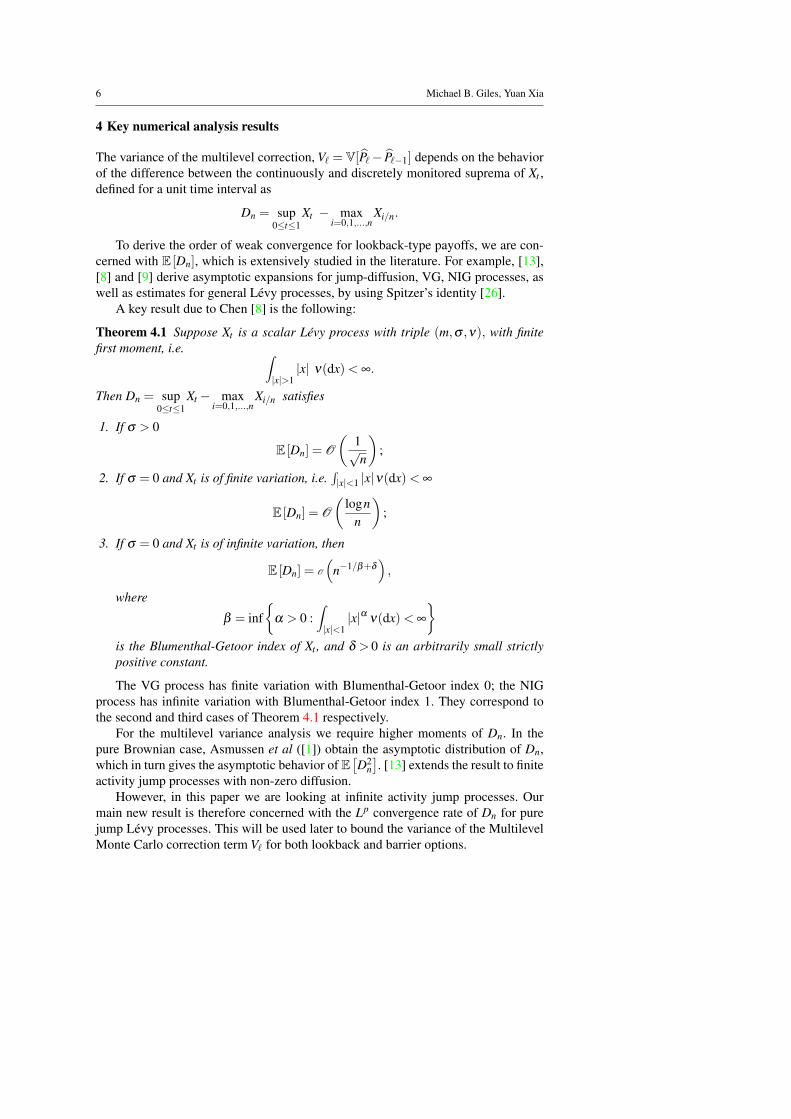
4 Key numerical analysis results

The variance of the multilevel correction, V` = V[P − P −1] depends on the behaviorof the difference between the continuously and discretely monitored suprema of Xt ,defined for a unit time interval as

Dn = sup0≤t≤1

Xt − maxi=0,1,...,n

Xi/n.

To derive the order of weak convergence for lookback-type payoffs, we are con-cerned with E [Dn], which is extensively studied in the literature. For example, [13],[8] and [9] derive asymptotic expansions for jump-diffusion, VG, NIG processes, aswell as estimates for general Levy processes, by using Spitzer’s identity [26].

A key result due to Chen [8] is the following:

Theorem 4.1 Suppose Xt is a scalar Levy process with triple (m,σ ,ν), with finitefirst moment, i.e. ∫

|x|>1|x| ν(dx)< ∞.

Then Dn = sup0≤t≤1

Xt − maxi=0,1,...,n

Xi/n satisfies

1. If σ > 0

E [Dn] = O

(1√n

);

2. If σ = 0 and Xt is of finite variation, i.e.∫|x|<1 |x|ν(dx)< ∞

E [Dn] = O

(logn

n

);

3. If σ = 0 and Xt is of infinite variation, then

E [Dn] = O

(n−1/β+δ

),

where

β = inf{

α > 0 :∫|x|<1|x|α ν(dx)< ∞

}is the Blumenthal-Getoor index of Xt , and δ > 0 is an arbitrarily small strictlypositive constant.

The VG process has finite variation with Blumenthal-Getoor index 0; the NIGprocess has infinite variation with Blumenthal-Getoor index 1. They correspond tothe second and third cases of Theorem 4.1 respectively.

For the multilevel variance analysis we require higher moments of Dn. In thepure Brownian case, Asmussen et al ([1]) obtain the asymptotic distribution of Dn,which in turn gives the asymptotic behavior of E

[D2

n]. [13] extends the result to finite

activity jump processes with non-zero diffusion.However, in this paper we are looking at infinite activity jump processes. Our

main new result is therefore concerned with the Lp convergence rate of Dn for purejump Levy processes. This will be used later to bound the variance of the MultilevelMonte Carlo correction term V` for both lookback and barrier options.


Theorem 4.2 Let Xt be a scalar pure jump Levy process, and suppose its Levy mea-sure ν(x) satisfies

C2 |x|−1−α ≤ ν(x)≤C1 |x|−1−α , for |x| ≤ 1;

ν(x)≤ exp(−C3 |x|) , for |x|> 1,(4.1)

where C1,C2,C3 > 0, 0≤ α < 2 are constants. Then for p≥ 1

Dn = sup0≤t≤1

Xt − maxi=0,1,...,n

Xi/n

satisfies

E [Dpn ] =

O( 1

n

), p > 2α;

O

((logn

n

) p2α

), p≤ 2α.

If, in addition, Xt is spectrally negative, i.e. ν(x) = 0 for x > 0, then

E [Dpn ] =

{O (n−p) , 0≤ α < 1;

O

(n−p/α+δ

), 1≤ α < 2;

for any δ > 0.

We will give the proof of this result later in Section 7.6. Note that for p=1, thegeneral bound in Theorem 4.2 is slightly sharper than Chen’s result for α < 1

2 , isthe same for α = 1

2 , and is not as tight as Chen’s result for 12 <α <2; the spectrally

negative bound is slightly sharper than Chen’s result for α <1, and the bound is thesame for 1≤α <2.

5 MLMC analysis

5.1 Asian options

We consider the analysis for a Lipschitz arithmetic Asian payoff P = P(S)

where

S = S0 T−1∫ T

0exp(Xt)dt .

and P is Lipschitz such that |P(S1)−P(S2)| ≤ LK |S1−S2|.

We approximate the integral using a trapezoidal approximation:

S := S0 T−1n−1

∑j=0

12 h(exp(X jh)+exp

(X( j+1)h

)), (5.1)

and the approximated payoff is then P = P(

S)

.


Proposition 5.1 Let Xt be a scalar Levy process underlying an exponential Levymodel. If S,S are as defined above, and

∫|z|>1 e2z ν(dz)< ∞, then

E[(

S−S)2]= O(h2).

The proof will be given later in Section 7.1. Using the Lipschitz property, theweak convergence for the numerical approximation is given by∣∣∣E[P −P

]∣∣∣≤ LKE[∣∣∣S`−S

∣∣∣]≤ LK

(E[(

S−S)2])1/2

,

while the convergence of the MLMC variance follows from

V` ≤ E[(

P − P −1

)2]

≤ 2 E[(

P −P)2]+2 E

[(P −1−P

)2]

≤ 2L2K E

[(S`−S

)2]+2L2

K E[(

S`−1−S)2].

5.2 Lookback options

In exponential Levy models, the moment generating function E[exp(qsup0≤t≤T Xt

)]can be infinite for large value of q. To avoid problems due to this, we consider alookback put option which has a bounded payoff

P = exp(−rT ) (K−S0 exp(m))+ , (5.2)

where m = sup0≤t≤T Xt . Note that P is a Lipschitz function of m, since we have|P′(x)| ≤ K. Without loss of generality, we assume T = 1 in the following.

Because of the Lipschitz property, we have∣∣∣E[P−P ]

∣∣∣≤ KE[Dn] where n=M`=

h−1` . Therefore we obtain weak convergence for the processes covered by Theorem

4.1, with the convergence rate given by the Theorem.To analyse the variance, V` = V[P −P −1], we first note that

0≤ max0≤i≤M`

Xi/M` − max0≤i≤M`−1

Xi/M`−1 ≤ sup0≤t≤1

Xt − max0≤i≤M`−1

Xi/M`−1 = Dn

where n = M`−1. Hence, we have

V` ≤ E[(

P − P −1

)2]≤ K2 E[D2

n].

Theorem 4.2 then provides the following bounds on the variance for the VG, NIGand spectrally negative α-stable processes.


Proposition 5.2 Let Xt be a scalar Levy process underlying an exponential Levymodel. For the Lipschitz lookback put payoff (5.2), we have the following multilevelvariance convergence rate results:

1. If Xt is a Variance Gamma (VG) process, then V` = O (h`);2. If Xt is a Normal Inverse Gaussian (NIG) process, then V` = O (h` |logh`|);3. If Xt is a spectrally negative α-stable process with α > 1, then V` = O

(h2/α−δ

`

),

for any small δ > 0.

5.3 Barrier options

We consider a bounded up-and-out barrier option with discounted payoff

P = exp(−rT ) f (ST) 1{sup0<t<T St<B} = exp(−rT ) f (ST) 1{m<log(B/S0)}, (5.3)

where again m = sup0<t<T Xt , and | f (x)|≤F is bounded. On level `, the numericalapproximation is

P = exp(−rT ) f (ST) 1{m`<log(B/S0)}. (5.4)

where m` = max0≤i≤M` Xih` .Our analysis for NIG and the spectrally negative α-stable processes requires the

following quite general result.

Proposition 5.3 If m is a random variable with a locally bounded density in a neigh-bourhood of B, and m is a numerical approximation to m, then for any p > 0 thereexists a constant Cp(B) such that

E[∣∣1{m<B}−1{m<B}

∣∣]<Cp(B) ‖m− m‖p/(p+1)p .

Proof This result was first proved by Avikainen (Lemma 3.4 in [2]), but we give herea simpler proof. If, for some fixed X >0, we have |m−B|> X and |m−m|< X , then1m<B−1m<B = 0. Hence,

E[ |1m<B−1m<B| ] ≤ P(|m−B| ≤ X)+P(|m−m| ≥ X)

≤ 2ρsup(B)X +X−p ‖m− m‖pp

with the first term being due to the local bound ρsup(B) of m’s density and the secondterm due to the Markov inequality. Differentiating the upper bound w.r.t. X , we findthat it is minimised by choosing X p+1 = p

2ρsup(B)‖m− m‖p

p, and we then get thedesired bound.

Our analysis for the Variance Gamma process requires a sharper result customisedto the properties of Levy processes.


Proposition 5.4 If Xt is a scalar pure jump Levy process satisfying the conditionsof Theorem 4.2 with 0 ≤ α ≤ 1

2 , and m and mn are the continuously and discretelymonitored suprema of Xt and m has a locally bounded density in a neighbourhood ofB, then

E[∣∣1{m<B}−1{m<B}

∣∣]= O(n−1/(1+2α)+δ ),

for any δ > 0.

The proof is given later in Section 7.7.

Both of the above propositions require the condition that the supremum m has alocally bounded density for all strictly positive values. There is considerable currentresearch on the supremum of Levy processes [6,7,21,22]. In particular, the com-ments following Proposition 2 in [7] indicate that the condition is satisfied by stableprocesses, and by a wide class of symmetric subordinated Brownian motions. Un-fortunately, the VG and NIG processes in the current paper are not symmetric, so atpresent they lie outside the range of current theory, but new theory under develop-ment [3] will extend the property to a larger class of Levy processes including bothVG and NIG.

We now bound the weak convergence of the estimator and the multilevel varianceconvergence.

Proposition 5.5 Let Xt be a scalar Levy process underlying an exponential Levymodel. For the up-and-out barrier option payoff (5.3), with the numerical approxi-mation (5.4), we have the following rates of convergence for the multilevel correctionvariance and the weak error, assuming that m has a bounded density:

– If Xt is a Variance Gamma (VG) process, then

V` = O(h1−δ

` );∣∣∣E[P−P]∣∣∣ = O(h1−δ

` )

where δ is an arbitrary positive number.– If Xt is a NIG process, then

V` = O(h1/2−δ

` );∣∣∣E[P−P]∣∣∣ = O(h1/2−δ

` )

where δ is an arbitrary positive number.– If Xt is a spectrally negative α-stable process with α > 1, then

V` = O

(h

1α−δ

`

);∣∣∣E[P−P

]∣∣∣ = O

(h

1α−δ

`

)where δ is an arbitrary positive number.


Proof The variance of the multilevel correction term is bounded by

V` ≤ E[(

P − P −1

)2]≤ 2 E

[(P −P

)2]+2 E

[(P −1−P

)2].

For an up-and-out Barrier option, since the payoff is bounded we have

E[(

P −P)2]≤ F2 E

[1{mn<log(B/S0)}−1{m<log(B/S0)}

],∣∣∣E[P −P

]∣∣∣ ≤ F E[1{mn<log(B/S0)}−1{m<log(B/S0)}

],

where n = M`.The bounds for the VG process come from Proposition 5.4 together with the

results from Theorem 4.2.The bounds for the NIG come from taking p=1 in Proposition 5.3 together with

Chen’s result Theorem 4.1.The bounds for the spectrally negative α-stable process come from Proposition

5.3 together with the results from Theorem 4.2. Theorem 4.2 gives

‖m−m‖p/(p+1)p ≡ (E [ |m−m|p])1/(p+1) = O(h

p(p+1)α−

δp+1 ).

We then obtain the desired bound by taking p to be sufficiently large.

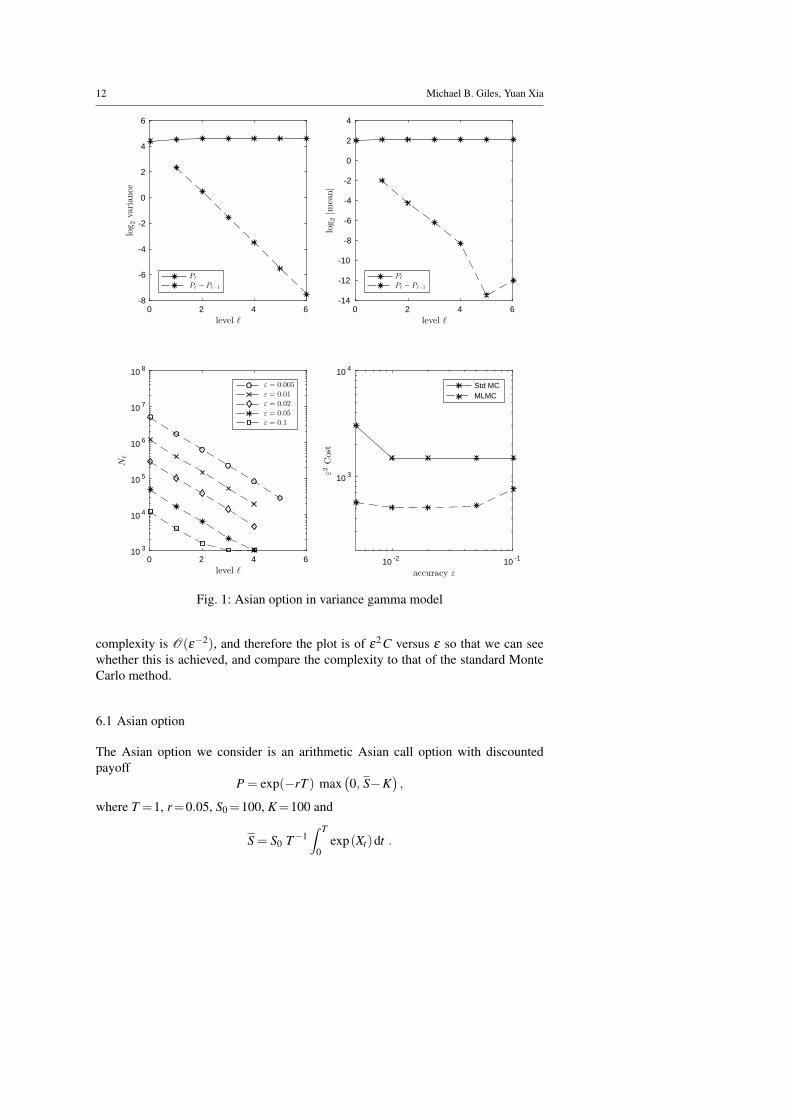
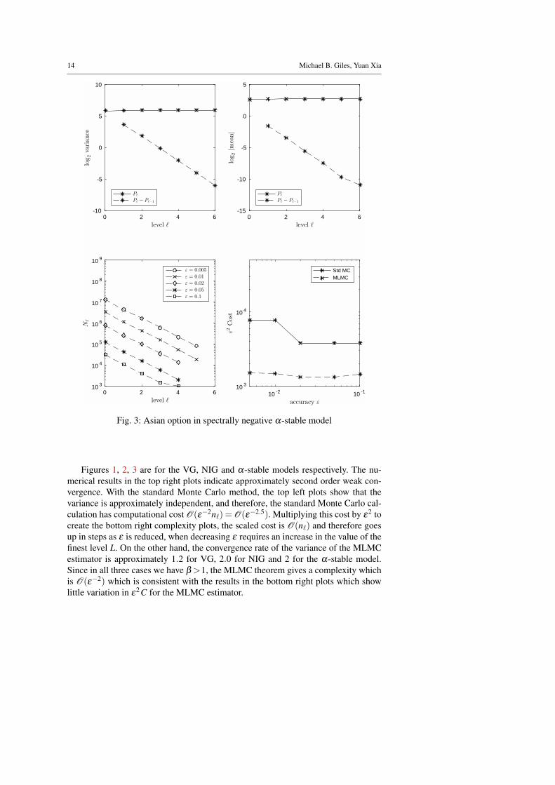
6 Numerical results

We have numerical results for three different Levy models: Variance Gamma, NormalInverse Gaussian and α-stable processes, and three different options: Asian, lookbackand barrier.

The current code is based on Giles’ MATLAB code [17], using which we generatestandardised numerical results and a set of four figures. The top two plots correspondto a set of experiments to investigate how the variance and mean for both P andP − P −1 vary with level `. The top left plot shows the values for log2(variance),so that the absolute value of the slope of the line for log2V[P −P −1] indicates theconvergence rate β of V` in condition i) of Thereom 2.1. Similarly, the absolute valueof the slope of the line for log2 |E[P −P −1]| in the top right plot indicates the weakconvergence rate α in the condition i) of Thereom 2.1.

The bottom two plots correspond to a set of MLMC calculations for different val-ues of the desired accuracy ε . Each line in the bottom left plot corresponds to onemultilevel calculation and displays the number of samples N` on each level. Notethat as ε is varied, the MLMC algorithm automatically decides how many levels arerequired to reduce the weak error appropriately. The optimal number of samples oneach level is based on an empirical estimation of the multilevel correction varianceV`, together with the use of a Lagrange multiplier to determine how best to minimisethe overall computational cost for a given target accuracy. A complete description ofthe algorithm is given in [19]. The bottom right plots show the variation of the com-putational complexity C with the desired accuracy ε . In the best cases, the MLMC


0 2 4 6level ℓ

-8

-6

-4

-2

0

2

4

6log2variance

Pℓ

Pℓ − Pℓ−1

0 2 4 6level ℓ

-14

-12

-10

-8

-6

-4

-2

0

2

4

log2|m

ean|

Pℓ

Pℓ − Pℓ−1

0 2 4 6level ℓ

10 3

10 4

10 5

10 6

10 7

10 8

Nℓ

ε = 0.005

ε = 0.01

ε = 0.02

ε = 0.05

ε = 0.1

10 -2 10 -1

accuracy ε

10 3

10 4

ε2Cost

Std MCMLMC

Fig. 1: Asian option in variance gamma model

complexity is O(ε−2), and therefore the plot is of ε2 C versus ε so that we can seewhether this is achieved, and compare the complexity to that of the standard MonteCarlo method.

6.1 Asian option

The Asian option we consider is an arithmetic Asian call option with discountedpayoff

P = exp(−rT ) max(0, S−K

),

where T =1, r=0.05, S0=100, K=100 and

S = S0 T−1∫ T

0exp(Xt)dt .


0 2 4 6level ℓ

-8

-6

-4

-2

0

2

4

6log2variance

Pℓ

Pℓ − Pℓ−1

0 2 4 6level ℓ

-20

-15

-10

-5

0

5

log2|m

ean|

Pℓ

Pℓ − Pℓ−1

0 2 4 6level ℓ

10 3

10 4

10 5

10 6

10 7

10 8

Nℓ

ε = 0.005

ε = 0.01

ε = 0.02

ε = 0.05

ε = 0.1

10 -2 10 -1

accuracy ε

10 3

10 4

ε2Cost

Std MCMLMC

Fig. 2: Asian option in Normal Inverse Gaussian model

For a general Levy process it is not easy to directly sample the integral process. Weuse the trapezoidal approximation

S := S0 T−1n−1

∑j=0

12 h (exp

(X jh)+exp

(X( j+1)h

)),

where n =T/h is the number of timesteps. The payoff approximation is then

P = exp(−rT ) max(

0, S−K).

In the multilevel estimator, the approximation P on level ` is obtained using n` :=2`

timesteps.


0 2 4 6level ℓ

-10

-5

0

5

10log2variance

Pℓ

Pℓ − Pℓ−1

0 2 4 6level ℓ

-15

-10

-5

0

5

log2|m

ean|

Pℓ

Pℓ − Pℓ−1

0 2 4 6level ℓ

10 3

10 4

10 5

10 6

10 7

10 8

10 9

Nℓ

ε = 0.005

ε = 0.01

ε = 0.02

ε = 0.05

ε = 0.1

10 -2 10 -1

accuracy ε

10 3

10 4

ε2Cost

Std MCMLMC

Fig. 3: Asian option in spectrally negative α-stable model

Figures 1, 2, 3 are for the VG, NIG and α-stable models respectively. The nu-merical results in the top right plots indicate approximately second order weak con-vergence. With the standard Monte Carlo method, the top left plots show that thevariance is approximately independent, and therefore, the standard Monte Carlo cal-culation has computational cost O(ε−2n`) =O(ε−2.5). Multiplying this cost by ε2 tocreate the bottom right complexity plots, the scaled cost is O(n`) and therefore goesup in steps as ε is reduced, when decreasing ε requires an increase in the value of thefinest level L. On the other hand, the convergence rate of the variance of the MLMCestimator is approximately 1.2 for VG, 2.0 for NIG and 2 for the α-stable model.Since in all three cases we have β >1, the MLMC theorem gives a complexity whichis O(ε−2) which is consistent with the results in the bottom right plots which showlittle variation in ε2 C for the MLMC estimator.


0 2 4 6level ℓ

-4

-3

-2

-1

0

1

2

3

4

5log2variance

Pℓ

Pℓ − Pℓ−1

0 2 4 6level ℓ

-4

-3

-2

-1

0

1

2

3

log2|m

ean|

Pℓ

Pℓ − Pℓ−1

0 2 4 6 8 10 12level ℓ

10 3

10 4

10 5

10 6

10 7

10 8

Nℓ

ε = 0.005

ε = 0.01

ε = 0.02

ε = 0.05

ε = 0.1

10 -2 10 -1

accuracy ε

10 3

10 4

10 5

10 6

ε2Cost

Std MCMLMC

Fig. 4: Lookback option with Variance Gamma model

For this Asian option, MLMC is 3-8 times more efficient than standard MC. Thegains are modest because the high rate of weak convergence means that only 4 levelsof refinement are required in most cases, so there is only a 24=16 difference in costbetween each MC path calculation on the finest level, and each of the MLMC pathcalculations on the coarsest level.

6.2 Lookback option

The lookback option we consider is a put option on the floating underlying,

P = exp(−rT )(

K− sup0≤t≤T

St

)+

= exp(−rT )(K−S0 exp(m))+ ,


0 2 4 6level ℓ

-4

-3

-2

-1

0

1

2

3

4

5log2variance

Pℓ

Pℓ − Pℓ−1

0 2 4 6level ℓ

-4

-3

-2

-1

0

1

2

3

log2|m

ean|

Pℓ

Pℓ − Pℓ−1

0 2 4 6 8 10 12level ℓ

10 3

10 4

10 5

10 6

10 7

10 8

Nℓ

ε = 0.005

ε = 0.01

ε = 0.02

ε = 0.05

ε = 0.1

10 -2 10 -1

accuracy ε

10 3

10 4

10 5

ε2Cost

Std MCMLMC

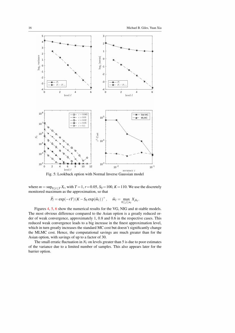
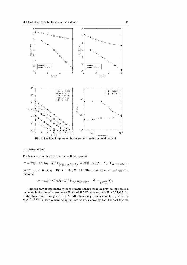
Fig. 5: Lookback option with Normal Inverse Gaussian model

where m = sup0≤t≤T Xt , with T =1, r=0.05, S0=100, K=110. We use the discretelymonitored maximum as the approximation, so that

P = exp(−rT )(K−S0 exp(m`))+ , m` = max

0≤ j≤n`X jh` .

Figures 4, 5, 6 show the numerical results for the VG, NIG and α-stable models.The most obvious difference compared to the Asian option is a greatly reduced or-der of weak convergence, approximately 1, 0.8 and 0.6 in the respective cases. Thisreduced weak convergence leads to a big increase in the finest approximation level,which in turn greatly increases the standard MC cost but doesn’t significantly changethe MLMC cost. Hence, the computational savings are much greater than for theAsian option, with savings of up to a factor of 30.

The small erratic fluctuation in N` on levels greater than 5 is due to poor estimatesof the variance due to a limited number of samples. This also appears later for thebarrier option.


0 2 4 6level ℓ

-3

-2

-1

0

1

2

3

4

5log2variance

Pℓ

Pℓ − Pℓ−1

0 2 4 6level ℓ

-3

-2

-1

0

1

2

3

log2|m

ean|

Pℓ

Pℓ − Pℓ−1

0 2 4 6 8 10 12level ℓ

10 3

10 4

10 5

10 6

10 7

10 8

10 9

Nℓ

ε = 0.005

ε = 0.01

ε = 0.02

ε = 0.05

ε = 0.1

10 -2 10 -1

accuracy ε

10 3

10 4

10 5

ε2Cost

Std MCMLMC

Fig. 6: Lookback option with spectrally negative α-stable model

6.3 Barrier option

The barrier option is an up-and-out call with payoff

P = exp(−rT )(ST−K)+ 1{sup0≤t≤T S(t)<B} = exp(−rT )(ST−K)+ 1{m<log(B/S0)},

with T =1, r=0.05, S0 =100, K=100, B=115. The discretely monitored approxi-mation is

P = exp(−rT )(ST−K)+ 1{m`<log(B/S0)}, m` = max0≤ j≤n`

X jh`

With the barrier option, the most noticeable change from the previous options is areduction in the rate of convergence β of the MLMC variance, with β ≈ 0.75,0.5,0.6in the three cases. For β < 1, the MLMC theorem proves a complexity which isO(ε−2−(1−β )/α), with α here being the rate of weak convergence. The fact that the


0 2 4 6level ℓ

-4

-2

0

2

4

6

8log2variance

Pℓ

Pℓ − Pℓ−1

0 2 4 6level ℓ

-6

-5

-4

-3

-2

-1

0

1

2

log2|m

ean|

Pℓ

Pℓ − Pℓ−1

0 2 4 6 8 10 12level ℓ

10 3

10 4

10 5

10 6

10 7

10 8

10 9

Nℓ

ε = 0.005

ε = 0.01

ε = 0.02

ε = 0.05

ε = 0.1

10 -2 10 -1

accuracy ε

10 3

10 4

10 5

ε2Cost

Std MCMLMC

Fig. 7: Barrier option in variance gamma model

MLMC complexity is not O(ε−2) is clearly visible from the bottom right complexityplots, but there are still significant savings compared to the standard MC computa-tions.


0 2 4 6level ℓ

-4

-2

0

2

4

6

8log2variance

Pℓ

Pℓ − Pℓ−1

0 2 4 6level ℓ

-6

-5

-4

-3

-2

-1

0

1

2

log2|m

ean|

Pℓ

Pℓ − Pℓ−1

0 2 4 6 8 10 12level ℓ

10 3

10 4

10 5

10 6

10 7

10 8

Nℓ

ε = 0.005

ε = 0.01

ε = 0.02

ε = 0.05

ε = 0.1

10 -2 10 -1

accuracy ε

10 3

10 4

10 5

ε2Cost

Std MCMLMC

Fig. 8: Barrier option in Normal Inverse Gaussian model

6.4 Summary and discussion

Table 1 summarizes the convergence rates for the weak error E[P−P] and the MLMCvariance V` = V[P −P −1] given by Propositions 5.1, 5.2, 5.5, and the empirical con-vergence rates observed in the numerical experiments.

In general, the agreement between the analysis and the numerical rates of conver-gence is quite good, suggesting that in most cases the analysis may be sharp. The mostobvious gap between the two is with the weak order of convergence for the Asian op-tion with all three models; the analysis proves an O(h) bound, whereas the numericalresults suggest it is actually O(h2). The numerical results are perhaps not surprisingas O(h2) is the order of convergence of trapezoidal integration of a smooth function,and therefore it is the order one would expect if the payoff was simply a multiple ofS.


0 2 4 6level ℓ

-1

0

1

2

3

4log2variance

Pℓ

Pℓ − Pℓ−1

0 2 4 6level ℓ

-5

-4

-3

-2

-1

0

1

log2|m

ean|

Pℓ

Pℓ − Pℓ−1

0 2 4 6 8 10 12level ℓ

10 3

10 4

10 5

10 6

10 7

10 8

10 9

Nℓ

ε = 0.005

ε = 0.01

ε = 0.02

ε = 0.05

ε = 0.1

10 -2 10 -1

accuracy ε

10 3

10 4

10 5

ε2Cost

Std MCMLMC

Fig. 9: Barrier option in spectrally negative α-stable model

7 Proofs

7.1 Proof of Proposition 5.1

Proof We decompose the difference between the true value and approximation intoparts which we can bound separately:

∣∣∣S− S∣∣∣ = S0 T−1

∣∣∣∣∣∫ T

0exp(Xt)dt −

n−1

∑j=0

12 h (exp

(X jh)+exp

(X( j+1)h

))

∣∣∣∣∣= S0 T−1

∣∣∣∣∣n−1

∑j=0

exp(X jh)∫ ( j+1)h

jh

(exp(Xt −X jh

)−1)

dt− 12 hexp(XT )+

12 h

∣∣∣∣∣.


Table 1: Convergence rates of weak error and variance V` for VG, NIG and α-stableprocesses; δ can be any small positive constant. The numerical values are estimatesbased on the numerical experiments.

VGnumerical analysis

option weak var weak varAsian O

(h2) O

(h2) O (h) O

(h2)

lookback O (h) O(h1.2) O (h |logh|) O (h)

barrier O(h0.8) O

(h0.9)

O

(h1−δ

)O

(h1−δ

)NIG

numerical analysisoption weak var weak varAsian O

(h2) O

(h2) O (h) O

(h2)

lookback O(h0.8) O

(h1.2)

O

(h1−δ

)O (h |logh|)

barrier O(h0.4) O

(h0.5)

O

(h0.5−δ

)O

(h0.5−δ

)spectrally negative α-stable with α > 1

numerical for α = 1.5597 analysisoption weak var weak varAsian O

(h2) O

(h2) O (h) O

(h2)

lookback O(h0.6) O

(h1.6)

O

(h1/α−δ

)O

(h2/α−δ

)barrier O

(h0.5) O

(h0.6)

O

(h1/α−δ

)O

(h1/α−δ

)

If we define

b j = exp(X jh),

I j =∫ ( j+1)h

jh

(exp(Xt−X jh

)−1)

dt,

RA = − 12 hexp(XT )+

12 h,

then

E[(

S−S)2]= T−2S2

0 E

∣∣∣∣∣n−1

∑j=0

b jI j +RA

∣∣∣∣∣2 ≤ 2T−2S2

0

E

∣∣∣∣∣n−1

∑j=0

b jI j

∣∣∣∣∣2+E

[R2

A] .

We have E[R2

A

]= O

(h2), and due to the independence of b j and I j we obtain

E

∣∣∣∣∣n−1

∑j=0

b jI j

∣∣∣∣∣2 = E

[n−1

∑j=0

b2j I

2j +2

n−1

∑m=1

m−1

∑j=0

bmImb jI j

]

=n−1

∑j=0

E[b2

j]E[I2

j]+2

n−1

∑m=1

m−1

∑j=0

E [bmImb jI j] . (7.1)


Defining A = 2m+∫ (

e2z−1−2z1|z|<1)

ν (dz), we have E[b2

j

]= eA jh. Furthermore,

by the Cauchy-Schwarz inequality,

E[I2

j]≤ h E

[∫ ( j+1)h

jh

(exp(Xt −X jh

)−1)2 dt

]= h

∫ h

0E[(exp(Xt)−1)2

]dt

= h(

1A

(eAh−1−Ah

)−2

1r

(erh−1− rh

))

Note that 1+ x < ex < 1+ x+ x2 for 0<x<1, and therefore for h<1/A we haveE[I2

j

]< Ah3 and hence

n−1

∑j=0

E[b2

j]E[I2

j]< Ah3

n−1

∑j=0

eA jh = AeAT −1eAh−1

h3 < (eAT−1) h2.

Now we calculate the second term in (7.1). Note that for m> j, Im is independentof bmb jI j, and bm/b j+1 is independent of b j+1b jI j, so

n−1

∑m=1

m−1

∑j=0

E [bmImb jI j] =n−1

∑m=1

E [Im]m−1

∑j=0

E[bm/b j+1

]E[b j+1b jI j

].

Firstly, for h < 1/r,

E [Im] =∫ h

0(ert −1) dt = r−1

(erh−1− rh

)< r h2.

Moreover, we have E[bm/b j+1

]= er(m− j−1)h and

E[b j+1b jI j

]=E

[exp(2X jh

)exp(X( j+1)h−X jh

)∫ ( j+1)h

jh

(exp(Xt−X jh

)−1)

dt]

=E[exp(2X jh

)]E[

exp(Xh)∫ h

0

(exp(Xt)−1

)dt]

= eA jh∫ h

0

(E [exp(Xh−Xt)]E [exp(2Xt)]−E [exp(Xh)]

)dt

= eA jh∫ h

0

(er(h−t)eAt − erh

)dt

= eA jherh e(A−r)h−1− (A−r)hA−r

.


Thus, for h < 1/(A−r),

n−1

∑m=1

m−1

∑j=0

E[bm/b j+1

]E[b j+1b jI j

]=

e(A−r)h−1− (A−r)A−r

n−1

∑m=1

m−1

∑j=0

er(m− j)heA jh

=e(A−r)h−1− (A−r)h(A−r)(e(A−r)h−1)

n−1

∑m=1

(eAmh− ermh)

< heAT −1eAh−1

< A−1(eAT −1).

Hence,

E

[n−1

∑m=1

m−1

∑j=0

bmImb jI j

]=

n−1

∑m=1

E [Im]m−1

∑j=0

E[bm/b j+1

]E[b j+1b jI j

]= O(h2),

and we can therefore conclude that E[(

S−S)2]= O(h2).

7.2 Levy process decomposition

The proofs rely on a decomposition of the Levy process into a combination of afinite-activity pure jump part, a drift part, and a residual part consisting of very smalljumps.

Let Xt be an (m,0,ν)-Levy process:

Xt = mt +∫ t

0

∫|z|≥1

z J(dz,ds)+∫ t

0

∫|z|<1

z(J(dz,ds)−ν(dz)ds) . (7.2)

The finite activity jump part is defined by

Xεt =

∫ t

0

∫ε<|z|

z J(dz,ds) =Nt

∑i=1

Yi

to be the compound Poisson process truncating the jumps of Xt smaller than ε whichis assumed to satisfy 0<ε <1. The intensity of Nt and the c.d.f. of Yi are

λε =∫

ε<|z|ν(dz). (7.3)

P(Yi < y) = λ−1ε

∫z<y

1{ε<|z|}ν(dz);

The drift rate for the drift term is defined to be

µε = m−∫

ε<|z|<1z ν(dz), (7.4)


so that the residual term is then a martingale:

Rεt :=

∫ t

0

∫|z|≤ε

z(J(dz,ds)−ν(dz)ds) . (7.5)

We define

σ2ε =

∫|z|≤ε

z2ν(dz), (7.6)

so that V [Rεt ] = σ2

ε t.These three quantities, µε , λε and σε will all play a major role in the subsequent

numerical analysis.We bound Dn by the difference between continuous maxima and 2-point maxima

over all timesteps:

Dn = sup0≤t≤1

Xt − maxi=0,1,...,n

X in≤ max

i=0,...,n−1D(i)

n (7.7)

where the random variables

D(i)n = sup

[ in ,

i+1n ]

Xt −max(

X i+1n,X i

n

)are independent and identically distributed. If we now define

∆(i)Xt = X i

n+t−X in, ∆

(i)Xεt = Xε

in+t−Xε

in, ∆

(i)t = t− in, ∆

(i)Rεt = Rε

in+t−Rε

in,

then

D(i)n = sup

[0, 1n ]

∆(i)Xt −

(∆(i)X 1

n

)+= sup

[0, 1n ]

(∆(i)Xε

t +∆(i)Rε

t +µε ∆(i)t)−(

∆(i)Xε

1n+∆

(i)Rε1n+µε

1n

)+

≤ sup[0, 1

n ]

(∆(i)Xε

t +∆(i)Rε

t

)−(

∆(i)Xε

1n+∆

(i)Rε1n

)++|µε |

n

≤ sup[0, 1

n ]

∆(i)Xε

t −(

∆(i)Xε

1n

)++|µε |

n+ sup

[0, 1n ]

∆(i)Rε

t +(−∆

(i)Rε1n

)+≤ sup

[0, 1n ]

∆(i)Xε

t −(

∆(i)Xε

1n

)++|µε |

n+2 sup

[0, 1n ]

∣∣∣∆ (i)Rεt

∣∣∣ (7.8)

where we use (a+b)+ ≤ a++b+ with a = ∆ (i)Xε1n+∆ (i)Rε

1n+µε

1n , b =−µε

1n in the

first inequality, and a = ∆ (i)Xε1n+∆ (i)Rε

1n

, b =−∆ (i)Rε1n

in the second inequality.


Let Z(i)n := sup[0, 1

n ]∆ (i)Xε

t −(

∆Xε1n

)+

and S(i)n := sup[0, 1n ]

∣∣∣∆ (i)Rεt

∣∣∣. Then, for p≥

1, Jensen’s inequality gives us

E [Dpn ]

≤E[

max0≤i<n

(Z(i)

n +|µε |

n+2S(i)n

)p]≤3p−1E

[max

0≤i<n

(Z(i)

n

)p+

(|µε |

n

)p

+2p max0≤i<n

(S(i)n

)p]

≤3p−1n E

sup[0, 1

n ]

Xεt −

(Xε

1n

)+p+3p−1(|µε |

n

)p

+3p−12pE[

max0≤i<n

(S(i)n

)p]

(7.9)

where in the final step we have used the fact that all of the ∆ (i)Xεt have the same

distribution as Xεt .

The task now is to bound the first and third terms in the final line of (7.9).

7.3 Bounding moments of sup[0, 1n ]

Xεt − (Xε

1n)+

Theorem 7.1 Let Xt be a scalar Levy process with a triple (m,0,ν), and let Xεt , µε ,

λε and σε be as defined in section 7.2.Then provided λε≤n, for any p>1 there exists a constant Kp such that

E

sup[0, 1

n ]

Xεt −

(Xε

1n

)+p≤ Kp

(ε

p +Lε (p)

λ 2ε

)λ 2

ε

n2 , (7.10)

where Lε (p) = p∫

x>εxp−1λ 2

x dx is a function depending on the Levy measure ν(x).

Proof Let

Z = sup[0, 1

n ]

Xεt −

(Xε

1n

)+.

We will determine an upper bound on E [Zp] by analysing the jump behavior ofthe finite-activity process Xε

t in a single interval [0, 1n ].

Let N be the number of jumps. If N≤ 1, then Z = 0, while if N = 2, then Z ≤min(|Y1| , |Y2|). This can be seen from the behavior of Xε

t in the different scenariosillustrated in Figure 10. More generally, if N=k, k≥2, then

Z > x =⇒ ∃ 1≤ j ≤ k−1 s.t.

∣∣∣∣∣ j

∑l=1

Yl

∣∣∣∣∣> x,

∣∣∣∣∣ k

∑l= j+1

Yl

∣∣∣∣∣> x

=⇒ ∃ j1, j2 s.t.∣∣Yj1

∣∣> xk−1

,∣∣Yj2

∣∣> xk−1

.


-

6

-

6

t

Xεt

t

Xεt

t

t

t

t

Fig. 10: Behavior of Xεt in the case of one or two jumps in the interval [0, 1

n ].

Since

P(∃ j1, j2 s.t.

∣∣Yj1

∣∣> xk−1

,∣∣Yj2

∣∣> xk−1

)≤ ∑

( j1, j2)P(∣∣Yj1

∣∣> xk−1

,∣∣Yj2

∣∣> xk−1

)

=k (k−1)

2P(|Y1|>

xk−1

)2

.

it follows that

E [Zp | N=k ] = p∫

xp−1P(Z > x | N=k)dx

≤ k (k−1)2

p∫

xp−1P(|Y1|>

xk−1

)2

dx

=k (k−1)

2p

λ 2ε

∫xp−1

(∫|z|>x/(k−1)

1{ε<|z|}ν(dz))2

dx

=k (k−1)p+1

2p

λ 2ε

∫xp−1

(∫|z|>x

1{ε<|z|}ν(dz))2

dx

≡ dk,p

(ε

p +Lε (p)

λ 2ε

), (7.11)

where dk,p =12 k (k−1)p+1. We then have

E [Zp] =∞

∑k=2

E [Zp | N=k] P(N=k)

≤(

εp +

Lε(p)λ 2

ε

)exp(−λε

n

)∞

∑k=2

dk,p

(λε

n

)k 1k!


For kp = dpe+2 there exists Cp such that for any k ≥ kp, dk,p ≤Cpk!

(k−kp)!, so

∞

∑k=2

dk,p

(λε

n

)k 1k!≤

kp−1

∑k=2

dk,p

(λε

n

)k 1k!

+Cp

∞

∑k=kp

(λε

n

)k 1(k− kp)!

≤kp−1

∑k=2

dk,p

(λε

n

)k 1k!

+Cp

(λε

n

)kp

exp(

λε

n

)≤ Kp

(λε

n

)2

for some constant Kp, where the last step uses the fact that λε≤n.Therefore, we obtain the final result that

E [Zp]≤ Kp

(ε

p +Lε (p)

λ 2ε

)(λε

n

)2

.

7.4 Bounding moments of sup[0,T ] |Rεt |

Proposition 7.2 Let Xt be a scalar Levy process with a triple (m,0,ν) and let Rεt ,

µε , λε and σε be as defined in section 7.2. Then Rεt satisfies

E

[sup[0,T ]|Rε

t |p

]≤

Kp

(T p/2σ

pε +T

∫|z|≤ε|z|p ν(dx)

), p > 2;

Kp T p/2σpε , 1≤ p≤ 2,

(7.12)

where Kp is a constant depending on p.

Proof For any 1≤ p≤2, by Jensen’s inequality and the Doob inequality (c.f. [24]),

E[

sup0≤t≤T

|Rεt |

p]≤ E

[sup

0≤t≤T|Rε

t |2]p/2

≤ 2pE[|Rε

T |2]p/2

= 2p T p/2σ

pε .

For any p>2, the Burkholder–Davis–Gundy inequality (c.f. [24]) gives

E[

sup0≤t≤1

|Rεt |

p]≤ E

[[Rε ]

p/21

]where [Rε ]t is the quadratic variation of Rε

t . We can use the method in pages 347-348of [24] to get

E[[Rε ]

p/21

]≤ Kp

[(∫|z|≤ε

z2ν(dz)

)p/2

+∫|z|≤ε

|z|p ν(dz)

]

= Kp

(σ

pε +

∫|z|≤ε

|z|p ν(dz))


where Kp is a constant depending on p.To extend this result to an arbitrary time interval [0,T ] we use a change of time

coordinate, t ′=t/T , with associated changed Levy measure ν ′(dz)=T ν(dz) to obtain

E

[sup[0,T ]|Rε

t |p

]≤ Kp

[T p/2

σp/2ε +T

∫|z|≤ε

|z|p ν(dz)].

7.5 Bounding moments of max0≤i<n S(i)n

Proposition 7.3 Let Xt be a scalar pure jump Levy process, with Levy measure ν(x)which satisfies

C2 |x|−1−α ≤ ν(x)≤C1 |x|−1−α , as |x| ≤ 1;

for constants C1,C2 > 0 and 0≤α<2. If S(i)n is as defined in section 7.2, and λε ≤ n,then for p≥1, and arbitrary δ >0 there exists a constant Cp,δ , which does not dependon n,ε such that

E[(

max0≤i<n

S(i)n

)p]≤Cp,δ ε

p−δ .

In the particular case of α =0, such a bound holds with δ =0.

Proof By Proposition 7.2, for q > 2,

E[(

max0≤i<n

S(i)n

)q]≤ n E

sup[0, 1

n ]

|Rεt |

q

≤ Kq

(n1−q/2

σqε +

∫|z|≤ε

|z|q ν(dx)).

Recalling the definition of σε (7.6), due to the assumption on ν(x) we have

σqε ≤

(2C1

2−α

)q/2

εq−qα/2,

∫|z|≤ε

|z|q ν(dx) ≤ 2C1

q−αε

q−α .

Given p≥ 1, for any q > max(2, p), Jensen’s inequality gives us

E[(

max0≤i<n

S(i)n

)p]≤ E

[(max

0≤i<nS(i)n

)q]p/q

≤ K p/qq

[(2C1

2−α

)q/2(ε−α

n

)q/2−1

+2C1

q−α

]p/q

εp−α p/q.

If α =0, then the desired bound is obtained immediately. On the other hand, if 0<α <2, then

λε ≥ C2

∫ε<|z|<1

1

|z|α+1 dz =2C2

α

(ε−α −1

).

Since λε≤n it implies that ε−α ≤ Kα

2C2n+1, and thus ε−α/n is bounded. Hence there

exists a constant C such that

E[(

max0≤i<n

S(i)n

)p]≤C ε

p−α p/q,

and by choosing q large enough so that α p/q≤ δ we obtain the desired bound.


7.6 Proof of Theorem 4.2

Proof Provided λε≤n, by (7.9) and (7.10) we have

E [Dpn ]≺ E

[(max

0≤i<nS(i)n

)p]︸︷︷︸

1)

+εp λ 2

ε

n︸︷︷︸2)

+Lε (p)

n︸︷︷︸3)

+

(|µε |

n

)p

︸︷︷︸4)

, (7.13)

where the notation u≺ v means there exists constant c > 0 independent of n such thatu < cv.

We can now bound each term, given the specification of the Levy measure, andif we can choose appropriately how ε → 0 as n→ ∞ so that the RHS of (7.13) isconvergent, then the convergence rate of E

[Dp

n]

can be bounded.For 0<x<1,

λx ≤ C1

∫x<|z|<1

1

|z|α+1 dz+∫

1<|z|exp(−C3 |z|) dz

≤

{2C1 log 1

x + l1, α = 0;

l2 x−α , 0 < α < 2.(7.14)

where l1, l2 are constants with l2 ≥ 2C−13 , while for x≥1,

λx ≤∫

x<|z|exp(−C3 |z|) dz = 2C−1

3 exp(−C3 x).

If α > 0, then

Lε(p) = p∫

x>ε

xp−1λ

2x dx

≤ l22 p∫

x>ε

xp−1 ( 1{x<1}x−2α +1{x>1} exp(−2C3x)

)dx

≤

l4, p > 2α;

l4 log 1ε+ l5, p = 2α;

l4ε−2α+p + l5, p < 2α.

(7.15)

where l3, l4, l5 are additional constants. If α = 0, it is easily verified that Lε(p) isbounded for p≥1, so (7.15) applies equally to this case.

Given 0<ε <1 we have

|µε | =∣∣∣∣m−∫

ε<|z|<1z ν(dz)

∣∣∣∣≤

|m|+ |C1−C2| ε1−α−1α−1 , α 6= 1;

|m|+ |C1−C2| log 1ε, α = 1.

(7.16)

Subject to the condition that λε ≤ n, we now have


1) By Proposition 7.3,

E[(

maxi=1,...,n

S(i)n

)p]≺ ε

p−δ , for any δ >0.

2) By (7.14),

εp λ 2

ε

n≺ n−1×

{ε p log 1

ε, α = 0;

ε p−2α , 0 < α < 2.

3) By (7.15),

Lε(p)n

≺ n−1×

1, p > 2α;

log 1ε, p = 2α;

ε−2α+p, p < 2α.

4) By (7.16),

(|µε |

n

)p

≺ n−p×

1+ |C1−C2|p ε p(1−α), α > 1;

1+(|C1−C2| log 1

ε

)p, α = 1;

1, α < 1.

In the following we assume C1 6=C2.

1. p≥ 2α .If we choose ε = C n−2/p, then λε ≺ ε−α ≺ n2α/p, and the constant C can betaken to be sufficiently small so that λε ≤ n for sufficiently large n.Taking δ < p/2, we find that the dominant contribution to (7.13) comes from 3),giving the desired result that

E [Dpn ]≺

{n−1, p > 2α;logn

n , p = 2α.

2. 1≤ p < 2α .

We can use Holder’s inequality to give E[Dp

n]≤ E

[D2α

n] p

2α ≺(

lognn

) p2α

.

For a spectrally negative process, sup[0, 1n ]

Xεt −(

Xε1n

)+

= 0, since Xt doesn’t have

positive jumps, and hence

E [Dpn ]≤ E

[(max

0≤i<nS(i)n

)p]+

(|µε |

n

)p

.

We can take ε = C n−1/α with the constant C again chosen so that λε ≤ n forsufficiently large n. We then obtain

E [Dpn ]≺

{n−p/α+δ , α ≥ 1;n−p, α < 1.

for any δ >0.


7.7 Proof of Proposition 5.4

We decompose the term we want to bound into parts and then balance their asymp-totic orders to get desired result.

Note that 1{mn<B} − 1{m<B} = 1 only if either m is close to the barrier or thedifference between discretely and continuously monitored maximum Dn = m− mn islarge. More precisely, {

1{mn<B}−1{m<B} = 1}⊂ F ∪G,

where F := {B≤ m≤ B+n−r} and G := {Dn > n−r} for an r > 0 to be determined.Hence

E[1{mn<B}−1{m<B}

]≤ P(F)+P(G) .

Due to the locally bounded density for m, P(F) = O (n−r).If we denote

Z(i)n = sup

[0, 1n ]

∆(i)Xε

t −(

∆(i)Xε

1n

)+.

where ∆ (i)Xt is as defined previously in Section 7.2, then (7.8) gives

Dn ≤ max0≤i<n

Z(i)n +

|µε |n

+ max0≤i<n

S(i)n

For α < 1, µε is bounded, so |µε | ≤ 12 n1−r, for sufficiently large n. Hence,

P(Dn > n−r) ≤ P

(max

0≤i<nZ(i)

n + max0≤i<n

S(i)n > 12 n−r

)≤ P

(max

0≤i<nZ(i)

n > 14 n−r

)+P

(max

0≤i<nS(i)n > 1

4 n−r).

Now, max0≤i<n Z(i)n > 0 requires that there are at least two jumps in one of the n

intervals. The probability of two jumps in one particular interval is

1− exp(− λε

n

)(1+ λε

n

)≺(

λε

n

)2

if λε ≤ n, and hence

P(

max0≤i<n

Z(i)n > 1

4 n−r)≺ λ 2

ε

n.

We use the Markov inequality for the remaining term. According to Proposition7.2, E

[max0≤i<n

(S(i)n

)p]≺ ε p−δ and so

P(

max0≤i<n

S(i)n > 14 n−r

)≺ E

[max

0≤i<n

(S(i)n

)p]/( 1

4 n−r)p ≺ εp−δ nrp.

Combining these elements, provided λε ≤ n, we have

E[1{mn<B}−1{m<B}

]≺ n−r + ε

p−δ nrp +λ 2

ε

n.


Equating the first two terms on the right hand side gives ε = n−r(1+p)/(p−δ ).

If α = 0, then λε ≺ log 1ε≺ logn, so λε = O(n) is satisfied. We also have λ 2

ε

n ≺(logn)2

n , and therefore for any r<1 we have E[1{mn<B}−1{m<B}

]≺ n−r.

If 0<α<2, then λε ≺ ε−α ≺ nrα(1+p)/(p−δ ), and hence λ 2ε

n ≺ n−1+2rα(1+p)/(p−δ ).Balancing n−r and n−1+2rα(1+p)/(p−δ ), gives λε = O(n) and

r =(

1+2α1+pp−δ

)−1

. (7.17)

Since r→ 11+2α

as δ→ 0, and p→∞, for any fixed value of r < 11+2α

it is possibleto choose appropriate values of p and δ to satisfy (7.17) and thereby conclude thatE[1{mn<B}−1{m<B}

]≺ n−r.

Acknowledgements This work was supported by the China Scholarship Council and the Oxford-Man In-stitute of Quantitative Finance. We would like to thank Ben Hambly, Andreas Kyprianou, Loic Chaumont,Jacek Malecki and Jose Blanchet for their helpful comments.

References

1. Asmussen, S., Glynn, P., Pitman, J.: Discretization error in simulation of one-dimensional reflectingBrownian motion. The Annals of Applied Probability 5(4), 875–896 (1995)

2. Avikainen, R.: Convergence rates for approximations of functionals of SDEs. Finance and Stochastics13(3), 381–401 (2009)

3. Blanchet, J.: personal communication (2015)4. Carr, P., Wu, L.: The Finite Moment Log Stable Process and Option Pricing. The Journal of Finance

58(2), 753–778 (2003)5. Chambers, J.M., Mallows, C.L., Stuck, B.: A method for simulating stable random variables. Journal

of the American Statistical Association 71(354), 340–344 (1976)6. Chaumont, L.: On the law of the supremum of Levy processes. The Annals of Probability 41(3A),

1191–1217. (2013)7. Chaumont, L., Malecki, J.: The asymptotic behavior of the density of the supremum of Levy pro-

cesses. Annales de l’Institut Henri Poincare (To appear)8. Chen, A.: Sampling error of the supremum of a Levy process. Ph.D. thesis, University of Illinois at

Urbana-Champaign (2011). URL https://www.ideals.illinois.edu/handle/2142/263219. Chen, A., Feng, L., Song, R.: On the monitoring error of the supremum of a normal jump diffusion

process. Journal of Applied Probability 48(4), 1021–1034 (2011)10. Cont, R., Tankov, P.: Financial modelling with jump processes. Chapman & Hall/CRC, London (2004)11. Dereich, S.: Multilevel Monte Carlo Algorithms for Levy-driven SDEs with Gaussian correction. The

Annals of Applied Probability 21(1), 283–311 (2011)12. Dereich, S., Heidenreich, F.: A multilevel Monte Carlo algorithm for Levy-driven stochastic differen-

tial equations. Stochastic Processes and their Applications 121(7), 1565–1587 (2011)13. Dia, E., Lamberton, D.: Connecting discrete and continuous lookback or hindsight options in expo-

nential Levy models. Advances in Applied Probability 43(4), 1136–1165 (2011)14. Ferreiro-Castilla, A., Kyprianou, A.E., Scheichl, R., Suryanarayana, G.: Multilevel Monte Carlo sim-

ulation for Levy processes based on the Wiener–Hopf factorisation. Stochastic Processes and theirApplications 124(2), 985–1010 (2014)

15. Figueroa-Lopez, J., Tankov, P.: Small-time asymptotics of stopped Levy bridges and simulationschemes with controlled bias. Bernoulli, 20(3), 1126–1164 (2014)

16. Giles, M.: Improved multilevel Monte Carlo convergence using the Milstein scheme. In: A. Keller,S. Heinrich, H. Niederreiter (eds.) Monte Carlo and Quasi-Monte Carlo Methods 2006, pp. 343–358.Springer-Verlag, Berlin Heidelberg New York (2007)

https://www.ideals.illinois.edu/handle/2142/26321


17. Giles, M.: Multilevel Monte Carlo path simulation. Operations Research 56(3), 607–617 (2008)18. Giles, M.B.: Multilevel Monte Carlo methods. In: Monte Carlo and Quasi-Monte Carlo Methods

2012. Springer-Verlag (2012)19. Giles, M.B.: Multilevel Monte Carlo methods. Acta Numerica 24, 259–328 (2015)20. Kuznetsov, A., Kyprianou, A., Pardo, J., Van Schaik, K.: A Wiener–Hopf Monte Carlo simulation

technique for Levy processes. The Annals of Applied Probability 21(6), 2171–2190 (2011)21. Kuznetsov, A.: On extrema of stable processes. The Annals of Probability 39(3), 1027–1060 (2011)22. Kwasnicki, M., Malecki, J., Ryznar, M.: Suprema of Levy processes. The Annals of Probability

41(3B), 2047–2065 (2013)23. Kyprianou, A.: Introductory lectures on fluctuations of Levy processes with applications. Springer

Verlag, Berlin Heidelberg New York (2006)24. Protter, P.: Stochastic integration and differential equations. Springer Verlag, Berlin Heidelberg New

York (2004)25. Schoutens, W.: Levy processes in finance: pricing financial derivatives. Wiley-Blackwell, New Jersey

(2003)26. Spitzer, F.: A combinatorial lemma and its application to probability theory. Trans. Amer. Math. Soc

82(2), 323–339 (1956)

multilevel monte carlo for exponential levy models´ · multilevel monte carlo for exponential levy...

Documents