multilevel modelling of event history data: comparing...
TRANSCRIPT

Stewart, Catherine H. (2010) Multilevel modelling of event history data: comparing methods appropriate for large datasets. PhD thesis. http://theses.gla.ac.uk/2007/ Copyright and moral rights for this thesis are retained by the author A copy can be downloaded for personal non-commercial research or study, without prior permission or charge This thesis cannot be reproduced or quoted extensively from without first obtaining permission in writing from the Author The content must not be changed in any way or sold commercially in any format or medium without the formal permission of the Author When referring to this work, full bibliographic details including the author, title, awarding institution and date of the thesis must be given
Glasgow Theses Service http://theses.gla.ac.uk/

Multilevel Modelling of Event History
Data: Comparing Methods Appropriate for Large Datasets
Catherine Helen Stewart
Submitted in fulfilment of the requirements for the Degree of Doctor of Philosophy
Department of Statistics Faculty of Information and Mathematical Sciences
University of Glasgow
2
Abstract
When analysing medical or public health datasets, it may often be of interest to
measure the time until a particular pre-defined event occurs, such as death from
some disease. As it is known that the health status of individuals living within
the same area tends to be more similar than for individuals from different areas,
event times of individuals from the same area may be correlated. As a result,
multilevel models must be used to account for the clustering of individuals
within the same geographical location. When the outcome is time until some
event, multilevel event history models must be used.
Although software does exist for fitting multilevel event history models, such as
MLwiN, computational requirements mean that the use of these models is
limited for large datasets. For example, to fit the proportional hazards model
(PHM), the most commonly used event history model for modelling the effect of
risk factors on event times, in MLwiN a Poisson model is fitted to a person-period
dataset. The person-period dataset is created by rearranging the original dataset
so that each individual has a line of data corresponding to every risk set they
survive until either censoring or the event of interest occurs. When time is
treated as a continuous variable so that each risk set corresponds to a distinct
event time, as is the case for the PHM, the size of the person-period dataset can
be very large. This presents a problem for those working in public health as
datasets used for measuring and monitoring public health are typically large.
Furthermore, individuals may be followed-up for a long period of time and this
can also contribute to a large person-period dataset. A further complication is
that interest may be in modelling a rare event, resulting in a high proportion of
censored observations. This can also be problematic when estimating multilevel
event history models.
Since multilevel event history models are important in public health, the aim of
this thesis is to develop these models so they can be fitted to large datasets
considering, in particular, datasets with long periods of follow-up and rare
events. Two datasets are used throughout the thesis to investigate three
possible alternatives to fitting the multilevel proportional hazards model in
MLwiN in order to overcome the problems discussed. The first is a moderately-

3
sized Scottish dataset, which will be the main focus of the thesis, and is used as
a ‘training dataset’ to explore the limitations of existing software packages for
fitting multilevel event history models and also for investigating alternative
methods. The second dataset, from Sweden, is used to test the effectiveness of
each alternative method when fitted to a much larger dataset. The adequacy of
the alternative methods are assessed on the following criteria: how effective
they are at reducing the size of the person-period dataset, how similar
parameter estimates obtained from using methods are compared to the PHM and
how easy they are to implement.
The first alternative method involves defining discrete-time risk sets and then
estimating discrete-time hazard models via multilevel logistic regression models
fitted to a person-period dataset. The second alternative method involves
aggregating the data of individuals within the same higher-level units who have
the same values for the covariates in a particular model. Aggregating the data
like this means that one line of data is used to represent all such individuals
since these individuals are at risk of experiencing the event of interest at the
same time. This method is termed ‘grouping according to covariates’. Both
continuous-time and discrete-time event history models can be fitted to the
aggregated person-period dataset. The ‘grouping according to covariates’
method and the first method, which involves defining discrete-time risk sets, are
both implemented in MLwiN and pseudo-likelihood methods of estimation are
used. The third and final method to be considered, however, involves fitting
Bayesian event history (frailty) models and using Markov chain Monte Carlo
(MCMC) methods of estimation. These models are fitted in WinBUGS, a software
package specially designed to make practical MCMC methods available to applied
statisticians. In WinBUGS, an additive frailty model is adopted and a Weibull
distribution is assumed for the survivor function.
Methodological findings were that the discrete-time method led to a successful
reduction in the continuous-time person-period dataset; however, it was
necessary to experiment with the length of time intervals in order to have the
widest interval without influencing parameter estimates. The grouping according
to covariates method worked best when there were, on average, a larger
number of individuals per higher-level unit, there were few risk factors in the
model and little or none of the risk factors were continuous. The Bayesian
4
method could be favourable as no data expansion is required to fit the Weibull
model in WinBUGS and time is treated as a continuous variable. However,
models took a much longer time to run using MCMC methods of estimation as
opposed to likelihood methods. This thesis showed that it was possible to use a
re-parameterised version of the Weibull model, as well as a variance expansion
technique, to overcome slow convergence by reducing correlation in the Markov
chains. This may be a more efficient way to reduce computing time than running
further iterations.

5
Table of Contents Abstract...................................................................................... 2 Acknowledgements........................................................................ 11 Author’s Declaration ...................................................................... 12 1 Introduction........................................................................... 13
1.1 The Use of Event History Models in Public Health ......................... 13 1.2 Introduction to Multilevel Modelling......................................... 14 1.3 Objectives ....................................................................... 16 1.4 Computing Hardware........................................................... 16 1.5 Overview of Thesis ............................................................. 17
2 Data Description...................................................................... 19 2.1 Introduction ..................................................................... 19 2.2 The Moderately-Sized Scottish Dataset...................................... 19 2.3 The Larger Swedish Dataset................................................... 22
3 Mental Health and Psychiatric Admissions in Scotland ......................... 24 3.1 Introduction to Mental Health in Scotland .................................. 24 3.2 Recording and Detecting Mental Disorder in Scotland .................... 26
3.2.1 The 12-item General Health Questionnaire (GHQ-12) ............... 27 3.3 Risk Factors for Psychiatric Admission....................................... 31
3.3.1 Demographic Predictors .................................................. 31 3.3.2 Socioeconomic Predictors................................................ 34 3.3.3 Lifestyle Predictors ....................................................... 37
3.4 Area Variations in Mental Illness ............................................. 39 3.5 Objectives using Scottish Health Survey Data .............................. 41
4 Psychiatric Admissions in Scotland: Some Exploratory Analyses ............. 43 4.1 Descriptive Statistics........................................................... 43
4.1.1 Psychiatric Admissions in the Scottish Health Survey................ 43 4.1.2 Distribution of GHQ-12 Score in the Scottish Health Survey ........ 45 4.1.3 Missing Data in the Scottish Health Survey ............................ 47
4.2 Applying Multilevel Modelling to Logistic Regression...................... 48 4.3 Results from Multilevel Logistic Regression................................. 51 4.4 Chapter Summary............................................................... 55
5 Multilevel Event History Modelling: A Review................................... 56 5.1 Introduction ..................................................................... 56 5.2 Single-Level Survival Modelling ............................................... 56
5.2.1 Introduction to Survival Modelling ...................................... 56 5.2.2 Proportional Hazards Model ............................................. 59 5.2.3 Accelerated Lifetime Model ............................................. 61
5.3 Multilevel Survival Modelling.................................................. 62 5.3.1 Extending the Single-Level Model....................................... 62 5.3.2 Software for Fitting Multilevel Models ................................. 63 5.3.3 Fitting a Multilevel Proportional Hazards Model in MLwiN .......... 64 5.3.4 Fitting a Multilevel Accelerated Lifetime Model in MLwiN.......... 73 5.3.5 Estimation of Parameters in MLwiN .................................... 74
5.4 Multilevel Survival Modelling in MLwiN: Results........................... 78 5.4.1 Introduction................................................................ 78 5.4.2 Results from Multilevel Continuous-Time Hazard Model ............ 81 5.4.3 Summary.................................................................... 84
5.5 Use of Multilevel Survival Models in Previous Studies ..................... 85 5.6 Chapter Summary............................................................... 88
6 Discussion: Findings from the Scottish Health Survey ......................... 91

6
6.1 Introduction ..................................................................... 91 6.2 Summary of Findings ........................................................... 91 6.3 Limitations....................................................................... 98
6.3.1 Limitations of Data........................................................ 98 6.3.2 Limitations of Variables and Analyses.................................101
6.4 Recommendations for Future Work .........................................103 6.5 Implications of the Findings..................................................104 6.6 Conclusions .....................................................................105
7 Alternative Methods for Fitting Multilevel Survival Models to Large Datasets 106
7.1 Introduction ....................................................................106 7.2 Defining Different Risk Sets ..................................................106
7.2.1 Introduction...............................................................106 7.2.2 The Multilevel Discrete-Time Model...................................108 7.2.3 Assumptions ...............................................................112 7.2.4 Estimation .................................................................113
7.3 Grouping According to Covariates...........................................113 7.3.1 Introduction...............................................................113 7.3.2 Continuous-Time Models ................................................115 7.3.3 Discrete-Time Models....................................................119
7.4 Bayesian Survival Models .....................................................123 7.4.1 Introduction to Bayesian Multilevel Survival Models ................123 7.4.2 Frailty Models.............................................................125 7.4.3 The Shared Frailty Model................................................126 7.4.4 Fitting Frailty Models in WinBUGS .....................................130 7.4.5 Estimating the Parameters in WinBUGS...............................136 7.4.6 Monitoring Convergence in WinBUGS..................................139
8 Fitting Alternative Methods to the Scottish Dataset: Results................145 8.1 Defining Different Risk Sets ..................................................145
8.1.1 Multilevel Discrete-Time Models with Equal Intervals of Time ....146 8.1.2 Multilevel Discrete-Time Models with Varied Intervals of Time...150 8.1.3 Summary: Defining Different Risk Sets ...............................154
8.2 Grouping According to Covariates...........................................155 8.2.1 Results from Grouping According to Covariates in Continuous Time 157 8.2.2 Results from Grouping According to Covariates in Discrete Time.161 8.2.3 Summary: Grouping According to Covariates........................165
8.3 Bayesian Survival Models .....................................................167 8.3.1 Proportional Hazards Models using a Bayesian Approach...........167 8.3.2 Fitting Frailty Models in WinBUGS .....................................170 8.3.3 Fitting Bayesian Frailty Models to a Simulated Dataset ............179 8.3.4 Reducing Correlation in the Weibull Model...........................183 8.3.5 Parameter Expansion in the Weibull Model ..........................205 8.3.6 Summary: Bayesian Frailty Models....................................212
8.4 Chapter Summary..............................................................214 9 Applying Alternative Methods to a Larger Dataset .............................219
9.1 Introduction ....................................................................219 9.2 Objectives using Swedish Data ..............................................219 9.3 Preliminary Analysis of Swedish Data.......................................220
9.3.1 Descriptive Statistics ....................................................220 9.3.2 Missing Data ...............................................................224 9.3.3 Results from Preliminary Analyses of Swedish Data.................225 9.3.4 Summary of Preliminary Analyses of Swedish Data..................230
7
9.4 Fitting Multilevel Survival Models to the Swedish Dataset...............230 9.4.1 Multilevel Continuous-Time Survival Models .........................231 9.4.2 Multilevel Discrete-time Survival Models .............................232 9.4.3 Grouping According to Covariates .....................................244 9.4.4 Bayesian Frailty Models..................................................250
9.5 Conclusions: Results from the Swedish Data..............................262 9.5.1 Summary of Findings from the Swedish Dataset .....................263 9.5.2 Limitations of the Data..................................................265
9.6 Conclusions: Suitability of Methods ........................................266 10 Discussion..........................................................................269
10.1 Introduction ....................................................................269 10.2 Summary of Methodological Findings .......................................270 10.3 Conclusions .....................................................................274 10.4 Implications of the Findings..................................................278 10.5 Limitations and Recommendations..........................................280
10.5.1 Methodological Limitations and Recommendations .................280 10.5.2 Other Limitations.........................................................282 10.5.3 Other Recommendations ................................................283
Appendix 1: 12-Item General Health Questionnaire (GHQ-12)....................284 Appendix 2: Checking the Proportional Hazards Assumption in the SHeS Data.285 Appendix 3: Trace Plots and Gelman-Rubin Plots from SHeS Weibull Model ...287 Appendix 4: WinBUGS Code for Re-parameterised Model with all Covariates ..291 Appendix 5: Discrete-Time Groupings for Swedish Dataset .......................293 Appendix 6: Checking the Proportional Odds Assumption in the Swedish Dataset..............................................................................................295 Appendix 7: Fitting a Discrete-Time Model with Five Risk Sets to the Swedish Dataset.....................................................................................297 Appendix 8: Trace Plots and Gelman-Rubin Plots from Swedish Weibull Model299 Appendix 9: WinBUGS code for the Weibull Model with Different Shape Parameters ................................................................................303 References.................................................................................304

8
List of Tables Table 2.1 - Variables in the Scottish dataset.......................................... 22 Table 2.2 - Variables in the Swedish dataset.......................................... 23 Table 4.1 - Psychiatric admission following survey interview ...................... 43 Table 4.2 - Psychiatric admission following survey interview by survey year .... 44 Table 4.3 - Psychiatric admission following survey interview by number of prior admissions .................................................................................. 45 Table 4.4 - Distribution of GHQ-12 score in SHeS .................................... 46 Table 4.5 - Psychiatric admission following survey interview by GHQ-12 score . 46 Table 4.6 - Results from multilevel logistic regression .............................. 53 Table 5.1 - Sample of SHeS Data before Expansion .................................. 69 Table 5.2 - Sample of SHeS Data after Expansion .................................... 69 Table 5.3 - Results from multilevel continuous-time hazard model ............... 82 Table 5.4 - Summary of multilevel survival modelling literature with large datasets..................................................................................... 86 Table 8.1 - Expanded dataset with equal discrete time intervals ................147 Table 8.2 - Results from ML discrete-time models with equal intervals .........148 Table 8.3 - Groupings for varying discrete time intervals..........................151 Table 8.4 - Expanded dataset with varying discrete time intervals ..............151 Table 8.5 - Results from ML discrete-time models with varying intervals .......153 Table 8.6 - Expanded dataset when grouping according to GHQ-12 score in continuous-time ..........................................................................158 Table 8.7 - Results from ML continuous-time models grouped according to GHQ-12 score ....................................................................................160 Table 8.8 - Percentage reduction when grouping covariates for continuous-time models .....................................................................................161 Table 8.9 - Expanded dataset when grouping according to GHQ-12 score in discrete-time..............................................................................162 Table 8.10- Results from ML discrete-time models grouped according to GHQ-12 score........................................................................................164 Table 8.11 - Percentage reduction when grouping covariates for discrete-time models with varying intervals ..........................................................165 Table 8.12 - Results from PH Models using a Bayesian Approach..................169 Table 8.13 - Results from Weibull model .............................................173 Table 8.14 - MC Error as a percentage of posterior standard deviation..........177 Table 8.15 - Comparing intercept-only models between all-event and highly censored simulated datasets ...........................................................180 Table 8.16 - Results from re-parameterised model fitted to simulated data ...186 Table 8.17 - Results from Weibull model with re-parameterisation ..............200 Table 8.18 - Results of re-parameterised Weibull model with variance expansion..............................................................................................207 Table 9.1 - Percentage of events by cohort year ....................................220 Table 9.2 - Percentage of events by socioeconomic risk factors ..................223 Table 9.3 - Results from preliminary analyses of Swedish data ...................226 Table 9.4 - Dividing time in the Swedish dataset....................................234 Table 9.5 - Discrete-time grouping for expanded dataset with 3 risk sets ......235 Table 9.6 - Discrete-time grouping for expanded dataset with 7 risk sets ......235 Table 9.7 - Results from fitting multilevel discrete-time models to Swedish data..............................................................................................236 Table 9.8 - Results from investigating the effect of cohort........................243

9
Table 9.9 - Percentage reduction in expanded dataset when grouping according to covariates ..............................................................................245 Table 9.10 - Results from grouping according to covariates with Swedish data 246 Table 9.11 - Results from fitting Bayesian frailty models to Swedish data .....252 Table 9.12 - MC error as a percentage of posterior standard deviation..........255 Table 9.13 - Results from fitting re-parameterised Weibull model with variance expansion to the Swedish dataset .....................................................259

10
List of Figures Figure 8.1 - Trace plots for GHQ-12 only model .....................................174 Figure 8.2 - Trace plots for full model ................................................175 Figure 8.3 - Gelman-Rubin plots for GHQ-12 only model...........................176 Figure 8.4 - Gelman Rubin Plots for full model ......................................176 Figure 8.5 - Trace plots for intercept-only models from all-event & highly censored simulated datasets ...........................................................180 Figure 8.6 - Gelman-Rubin plots for intercept-only models from uncensored & highly censored simulated datasets ...................................................181 Figure 8.7 - Trace plots for re-parameterised model fitted to simulated dataset with no censoring.........................................................................189 Figure 8.8 - Trace plots for re-parameterised model fitted to simulated dataset with censoring ............................................................................192 Figure 8.9 - Gelman-Rubin plots for re-parameterised model fitted to simulated dataset with no censoring...............................................................194 Figure 8.10 - Gelman-Rubin plots for re-parameterised model fitted to simulated dataset with censoring ..................................................................195 Figure 8.11 - Trace plots for re-parameterised GHQ-12 model....................201 Figure 8.12 - Trace plots for re-parameterised full model.........................202 Figure 8.13 - Gelman-Rubin plots for re-parameterised GHQ-12 model .........203 Figure 8.14 - Gelman-Rubin plots for re-parameterised full model...............203 Figure 8.15 - Trace plots for re-parameterised GHQ-12 model with variance expansion ..................................................................................208 Figure 8.16 - Trace plots for re-parameterised full model with variance expansion ..................................................................................209 Figure 8.17 - Gelman-Rubin plots for re-parameterised GHQ-12 model with variance expansion.......................................................................210 Figure 8.18 - Gelman-Rubin plots for re-parameterised full model with variance expansion ..................................................................................210 Figure 9.1 - Date of event by birth cohort year......................................221 Figure 9.2 - Trace plots for 'Individual+Area' Model .................................253 Figure 9.3 - Gelman-Rubin plots for 'Individual+Area' model ......................253 Figure 9.4 - Trace plots for 'Individual+Area+Time*Cohort' Model ................254 Figure 9.5 - Gelman-Rubin plots for 'Individual+Area+Time*Cohort' Model ......254 Figure 9.6 - Trace plots for re-parameterised Weibull model with variance expansion ..................................................................................260 Figure 9.7 - Gelman-Rubin plots for re-parameterised Weibull model with variance expansion.......................................................................261

11
Acknowledgements
Firstly I would like to acknowledge the Medical Research Council Social & Public
Health Sciences unit for funding this PhD and the Statistics Department for their
continued support.
Thank you to my supervisors, Professor Alastair Leyland and Professor Mike
Titterington, for their continual help, support and guidance over the years. It
has been a privilege to work with such highly-respected researchers. I would also
like to acknowledge Dr Agostino Nobile for his input, and Dr Göran Henriksson for
providing data.
I owe a big thank you to my proof-readers; Carolyn, Chris, Denise, Ruth and my
dad, Robert. Your comments have been very much appreciated during these
final stages. I would also like to thank my fellow-PhD students; Alison, Caroline,
Emily and Kalonde. Sharing an office with you all has provided me with a lot of
laughter and support over the years and because of this I have lots of fond
memories of doing my PhD.
Outside of university I would especially like to thank my parents, Catherine and
Robert. Without their support and encouragement I would never have had the
confidence to embark on a PhD. I hope I have made you both proud. Thanks to
my brother, Gavin and my sister-in-law, Myla, for their support also.
Finally, I would like to say thank you to Chris for being so patient and
understanding during the final stressful stages of the PhD. You have given me
many happy times over the last three years.

12
Author’s Declaration
Results in Section 5.4 have been published (Gray L, Batty GD, Craig P, Stewart C,
Whyte B, Findlayson B, Leyland AH. Cohort Profile: The Scottish Health Surveys
Cohort: linkage of study participants to routinely collected records for
mortality, hospital discharge, cancer and offspring birth characteristics in three
nationwide studies. International Journal of Epidemiology, 2010. 39(2): p. 345-
350.)

13
1 Introduction
1.1 The Use of Event History Models in Public Healt h
When analysing medical or public health datasets, it may often be of interest to
measure the time until a particular pre-defined event occurs, such as death from
a particular disease. This time is known as the survival time. Event history
models are applied when the outcomes are measures of duration. In general, the
fundamental aim of event history analysis is to use data to provide estimates of
the probability of surviving beyond a specified time. This probability is known as
the ‘survivor function’. It has been shown, however, that survival data are
modelled more appropriately through the ‘hazard function’. The term ‘hazard’ is
used to describe the concept of the risk of ‘failure’ in an interval after time t,
conditional on the subject having survived to time t [1]. With event history data,
there may be information available on a number of explanatory variables
suspected to have an effect on the time until event. The proportional hazards
and accelerated lifetime models are the most commonly used models for
regressing the time until event on potential explanatory variables in public
health.
One of the main features of event history models is their ability to deal with
incomplete observations of survival time, referred to as ‘censored’ observations.
The most commonly encountered censoring mechanism in public health is ‘right-
censoring’. Right-censoring implies that it is known only that an individual has
not experienced the event of interest by the end of a period of follow-up. Other
types of censoring include ‘left-censoring’ and ‘interval-censoring’.
For many outcomes, the health of individuals has been shown to vary between
areas and this can also be true for event times. In such circumstances it is
important that the data are analysed using multilevel models. Hence, in the case
of event history data, multilevel event history models should be employed.

Chapter 1
14
1.2 Introduction to Multilevel Modelling
There is a growing amount of research in epidemiology and public health into
the relationship between characteristics of places where people live and health
outcomes. This is creating widespread acceptance that health varies across
geographic locations [2].
Although the focus on the importance of area variations in health outcomes has
changed over time, the concept is not new. Initially, public health and early
epidemiological investigations of infectious diseases were fundamentally
ecological, and were interested in the associations of health and disease with
environmental and community characteristics [3]. An example of this was John
Snow’s study of cholera, which concluded that geographical setting was key to
the spread of cholera in London [4].
Conversely, between the mid 1940s to the early 1990s, modern epidemiology
focused more on individual-level factors rather than environmental factors [5].
One reason for this shift was the increased prominence of chronic disease in this
century, with research focusing mainly on behavioural and biological
characteristics responsible for chronic disease [3]. A second reason concerned
the ‘ecological fallacy’. The ecological fallacy occurs when associations found at
the group level are inferred to the individual level when, in truth, no such
association exists [3, 6, 7]. The ecological fallacy arose as a result of ecological
studies used in the ‘pre-modern phase of epidemiology’ [8].
Since the 1980s and early 1990s, there has been renewed interest in the
importance of the effect of context on health outcomes [9]. The ‘new public
health’ seeks to bring the focus of public health research ‘back towards
structural and environmental influences on health and health behaviours’ [5].
Duncan, Jones and Moon [10] argued that, as well as recognising the health risks
of the present day being associated with individual behavioural choices, they
should also be regarded as being part of the broader social world. Health
outcomes may be affected by contextual effects associated with a particular
geographical location, or variations in health outcomes may be a result of
compositional effects, whereby particular types of individuals, who are more

Chapter 1
15
susceptible to poor health outcomes due to their individual characteristics, are
clustered in particular geographical locations [11].
As discussed earlier, it is widely accepted that health varies across geographical
locations. Instinctively, individuals within the same area tend to be more similar
in health status than individuals from different areas [12]. This clustering of
individuals within areas leads to a correlation of health outcomes for individuals
within the same area, demonstrating the shared experiences of individuals
within the same area [13]. This correlation structure leads to the violation of
the assumption of independence required for common regression techniques,
which in turn leads to underestimation of standard errors [13]. In addition, the
finding of differences and relationships when they do not actually exist is also
more likely [14].
Data that fall into hierarchies can be analysed using multilevel models, which
account for the dependence of outcomes of people within the same area [12]
[13]. Multilevel models allow the total variation in the response, which is
measured at the individual level, to be partitioned into variation attributable to
individual factors and variation that is attributable to differences between areas
[7, 13].The contribution of individual-level characteristics and area-level
characteristics to the total variation in the response can then be measured
simultaneously. Not only do multilevel models overcome the ecological fallacy
defined earlier, they also overcome the ‘atomistic’ or ‘individualistic’ fallacy.
The atomistic fallacy occurs when associations found between an outcome and
an individual characteristic are inferred to the group-level, when in truth this
association does not exist [3, 7].
Although multilevel modelling has appeared and reappeared over the last 50
years in a variety of forms [15], it was in the 1980s that notable developments in
multilevel modelling occurred, in particular, in the field of educational research
[16]. It is only in the last fifteen years that it has become more widely used in
the field of public health [17], partly to deal with the problem of the ecological
fallacy [18]. However, developments in statistical computing capabilities have
now made multilevel models accessible to researchers from a number of
different fields of research [19].

Chapter 1
16
1.3 Objectives
When analysing event history data that fall into hierarchies, multilevel event
history models should be used in order to account for the dependence of survival
times of individuals nested within the same area. Although multilevel event
history models have been developed, computational requirements mean that
their use is limited for large datasets. This poses a problem for those working in
the field of public health since datasets used for measuring and monitoring
public health are typically large, coming from routine sources such as hospital
discharge records or death records, or from survey sources. Additionally,
depending on the outcome of interest and the length of follow-up, there may be
relatively few events resulting in a large proportion of censored observations.
Having many censored observations can also become problematic when
estimating multilevel event history models.
The main objective of this thesis is therefore to investigate ways in which
multilevel event history models can be developed to model large datasets. In
particular, datasets with long periods of follow-up and cases where the outcome
of interest is rare, implying a high proportion of censored observations, will be
considered. Specifically, this research will consider limitations of existing
software packages for fitting multilevel event history models and alternative
strategies or software which may be applied instead.
1.4 Computing Hardware
All analyses in the thesis will be performed on a Dell OptiPlex 755 desktop
computer with Intel® Core™ 2 Duo processor; processor speed 1.95 GHz and 2048
MB of RAM.

Chapter 1
17
1.5 Overview of Thesis
The following chapter introduces datasets to which multilevel event history
models will be fitted in order to investigate, firstly, the limitations of existing
software packages for fitting these models and secondly, alternative strategies
which could be applied.
Chapter 3 introduces the first research question which will be the main focus for
the majority of the thesis. Background information detailing the context and
specific aims to be investigated will be covered, as well as a thorough review of
existing literature that has previously addressed this research question.
In Chapter 4, some initial investigations of the moderately-sized dataset being
used to analyse the first research question are conducted. Specifically, this
includes descriptive statistics and some preliminary analysis using multilevel
logistic regression.
Chapter 5 introduces event history models, showing how a single-level model can
be extended to incorporate random effects to fit multilevel models. A summary
of existing software for fitting multilevel event history models is included, with
a particular focus on MLwiN [20]. A detailed account of how MLwiN can be used
to fit multilevel continuous-time event history models is given, along with some
potential limitations of this package. This is demonstrated through fitting
multilevel continuous-time event history models to the moderately-sized dataset
being analysed to address the first research question. A brief summary of
modelling strategies and software used in previous studies for fitting multilevel
event history models to large datasets is also included.
Detailed conclusions for the first research question, as well as limitations of the
dataset being analysed and the analyses performed to address this research
question are considered in Chapter 6. Recommendations for future work and
implications of the findings are also covered here.
Chapter 7 considers other potential methods which may be used as an
alternative to fitting multilevel continuous-time event history models. In
particular, other strategies which could be utilised in MLwiN are considered. The

Chapter 1
18
latter part of this chapter discusses the use of WinBUGS [21] for fitting
multilevel event history models using a Bayesian approach.
In Chapter 8, the alternative methods considered in Chapter 7 are fitted to the
moderately-sized dataset being used to address the first research question.
Results from fitting alternative methods are compared to the standard
continuous-time models discussed in Chapter 5. The alternative methods are
then assessed to determine whether they are adequate substitutes for fitting
multilevel continuous-time event history models.
Chapter 9 introduces a much larger dataset which is then used to demonstrate
how effective the alternative methods discussed in Chapter 7 are when fitted to
a dataset with a larger number of individuals and a longer period of follow-up.
Finally, Chapter 10 discusses overall conclusions which can be drawn from the
thesis. Methodological implications of the findings for those working in the field
of public health are considered, as well as limitations of the research and
recommendations for further research.

19
2 Data Description
2.1 Introduction
This chapter gives an overview of the datasets which will be used to investigate
ways of fitting multilevel event history models. Two datasets will be analysed
over the course of the thesis. The first is a moderately-sized Scottish dataset
which will be used as a ‘training’ dataset for, firstly, investigating how
multilevel continuous-time event history models can be fitted in MLwiN, along
with the limitations of this software for fitting these models and secondly, for
testing alternative strategies to fitting continuous-time models which can be
utilised both in MLwiN, and in other packages. The Scottish training dataset will
be the main focus for the majority of the thesis. Once effective alternative
methods have been established using the training dataset, they will then be
applied to a Swedish dataset consisting of a much larger number of individuals
who were followed up for a much longer period of time compared with the
Scottish dataset. As the Swedish dataset will only be used to see how effective
alternative methods are when applied to a much larger dataset, the dataset and
research questions to be analysed will not be considered in as much depth as the
Scottish dataset.
2.2 The Moderately-Sized Scottish Dataset
This section introduces the Scottish dataset which will be used as the training
dataset as described in Section 2.1 above. The data come from the 1995 and
1998 Scottish Health Surveys (SHeS), and were linked to all death records and
psychiatric hospital admission records (Scottish Morbidity Record 04 (SMR04))
[22].
The 1995 and 1998 Scottish Health Surveys are the first two of a series of
ongoing general health surveys being conducted in Scotland. Before the
introduction of the Scottish Health Survey (SHeS) in 1995 there was a paucity of
systematic information on health and health-related behaviour available in

Chapter 2
20
Scotland to allow researchers to investigate reasons for variations in mortality
and morbidity in the Scottish population [23]. The series of surveys,
commissioned by The Scottish Executive Health Department (formerly The
Scottish Office Department of Health) was designed to rectify this lack of
knowledge.
The SHeS is modelled on the annual Health Survey for England in terms of the
core questions and measurements recorded. Therefore, in addition to allowing
the investigation of explanations for variations in mortality in Scotland,
differences between Scotland and England may also be investigated.
A wide range of information on health-related factors (e.g. long-standing illness,
recent diagnoses, prescribed medicines), behavioural variables (e.g. smoking,
physical activity) and biological measurements (e.g. blood pressure, BMI) were
recorded by the survey via an interview and a nurse visit [24]. Information on
deprivation and socioeconomic characteristics was measured both at the
individual-level and the household-level. The sample was designed to provide a
nationally representative sample of the working-age population of Scotland in
private households and is based on a stratified multistage random sample design
covering all of mainland Scotland as well as the larger inhabited islands [23, 25].
Postcode sectors within Scotland were ordered by region (seven regions defined
by Health Board) and deprivation (using the Carstairs index of deprivation [26]),
with 312 postcode sectors then being selected each year. Within the 312
sampled postcode sectors, 14 358 and 15 288 addresses were selected for the
1995 and 1998 surveys respectively using the Postcode Address File (PAF) [23,
25]. There were slight differences between the 1995 and 1998 surveys when
proceeding to select households and individuals from the random sample of
addresses. In the 1995 survey, one person aged 16-64 was randomly selected for
inclusion at each address containing a private household. However, in the 1998
survey up to three private households at each address could be selected. The
age limits were also changed so that anyone aged 2-74 was eligible for inclusion.
In each private household one person aged 16-74 and up to two children aged 2-
15 were randomly selected for inclusion. However, in this thesis, analyses will be
based only on subjects aged 16-74 years, i.e. children will be excluded. This
multistage clustered design is a commonly used sampling method in national
Chapter 2
21
surveys and is more cost-effective than designs without clustering, such as
simple random sampling [27].
Data from the Scottish Health Survey were obtained for use in the thesis by
means of a data application request to the Information and Services Division
Scotland (ISD Scotland). On applying for the survey data, all psychiatric hospital
admission records (SMR04), as well as all death records were requested in the
form of a linked dataset. The SMR04 is used to collect patient based data on day
cases and inpatient admissions, readmissions and discharges from psychiatric
hospitals and units.
Linkage of the 1995 and 1998 SHeS data to Scottish hospital admission records
and death records began in 2004 [27]. For those survey respondents who gave
permission to be linked to the NHS administrative database, survey data were
linked with all Scottish hospital records and death records from the year 1981 to
2004 [27]. Linkage was successful with around 92% of respondents in each of the
1995 and 1998 surveys agreeing to have their survey data linked to the NHS
administrative database [24]. The linkage procedure is summarised briefly as
follows [28]. For all respondents who agree to linkage, the National Centre for
Social Research (NCSR) send a datafile containing details of respondent’s name,
postcode, date of birth and year of participation in survey, along with an
encrypted serial number, to ISD Scotland for linkage with hospital records and
death records using probability matching techniques [29]. Following
anonymisation, these linked records are then forwarded to NHS Health Scotland
(formerly the Public Health Institute of Scotland). In addition, NCSR provide NHS
Health Scotland with a datafile containing all survey data and the same
encrypted serial number. The encrypted serial number thus allows merging of
survey data and the linked hospital and death records. The final merged dataset,
which does not include the encrypted serial number, is then sent back to and
stored by ISD Scotland. A primary benefit of data linkage includes being able to
investigate relationships between risk factors measured in the health survey and
hospital admissions or mortality [24]; however, there are also some weaknesses
associated with using linked datasets for analysis. These will be considered in
Section 6.3.1.

Chapter 2
22
When requesting the linked datasets from ISD Scotland, a description of all
survey variables required was also included in the application. Although many
variables were available, only those shown in Table 2.1 below were requested.
Table 2.1 - Variables in the Scottish dataset
The data were received from ISD Scotland in April 2006. All cleaning and merging
of the 1995 and 1998 linked datasets was done at this time for a dissertation
submitted in August 2006 as part of the University of Glasgow Master of Public
Health degree [30].
2.3 The Larger Swedish Dataset
This section introduces the Swedish dataset being used to test the effectiveness
of the alternative methods when fitted to a much larger dataset. Only a brief
overview is given here since this dataset is not the main focus of the thesis.
The Swedish dataset consists of two birth cohorts from the years 1972 and 1977,
containing 99458 and 86505 individuals respectively. Individuals were followed
up until at least 2003 with the last date of follow-up in 2006. It is clear from this
that the Swedish dataset is much larger than the Scottish dataset, in terms of
both the number of individuals and the length of follow-up time.
Like the Scottish dataset, the Swedish dataset is hierarchically structured, with
the 185963 individuals nested within 2596 parishes, which are in turn nested

Chapter 2
23
within 280 municipalities. Early-life socioeconomic variables at both the
individual-level and the higher-levels were available, as displayed in Table 2.2.
Table 2.2 - Variables in the Swedish dataset
The Swedish dataset is provided courtesy of Dr Göran Henriksson, University of
Gothenburg.

24
3 Mental Health and Psychiatric Admissions in
Scotland
A current and increasing health problem in Scotland is that of mental illness.
Using the linked Scottish Health Survey (SHeS), this thesis will investigate those
at risk of mental health problems in Scotland. This chapter provides an overview
of the extent of mental health problems in Scotland, and how mental health
problems are recorded and detected. Later sections of this chapter provide a
review of the literature for risk factors associated with poor mental health. The
final section of this chapter sets out the objectives to be considered when
analysing the SHeS data.
3.1 Introduction to Mental Health in Scotland
The World Health Organisation (WHO) defines health as ‘a state of complete
physical, mental and social well-being and not merely the absence of disease or
infirmity’ [31]. The Scottish Public Mental Health Alliance [32] noted that,
throughout the last century, there was an improvement in physical health in
Scotland and remarked that even mortality from illnesses such as heart disease
and cancer declined. However, they observed that the pattern of disease in the
industrialised world is changing, with poor mental health, as opposed to poor
physical health, being the main burden of ill-health in Scotland today. In order
to improve health to comply with the WHO’s definition, the new challenge for
the 21st century must be to focus on improving mental health and well-being.
In Scotland, it has been estimated that one in four people will experience
problems with mental wellbeing during their lifetime, and a recent survey
revealed that 62% of Scots knew of someone who had been diagnosed as being
mentally ill [33]. To highlight the costs of mental health problems to society and
the economy in Scotland, a report entitled ‘What’s it Worth?’ was launched in
2006. The report found that the total cost of mental health problems in Scotland
in 2005 was £8.6 billion, which was more than the total amount spent by the
National Health Service (NHS) in Scotland for all other health conditions

Chapter 3
25
combined [34]. The document ‘With Health in Mind: Improving mental health
and wellbeing in Scotland’ [32] provides a further insight into the costs of
mental health problems in Scotland, in particular, the cost to industry. It
reported that around 3 in 10 employees experience mental health problems each
year. Further research commissioned by the Scottish Association for Mental
Health [35] reported that the cost of absence as a result of mental health
problems to Scotland’s employers was around £360 million.
Definitions of mental disorder expand to include anything from conditions such
as depression and schizophrenia to alcohol and drug abuse. The terminology used
to describe poor mental health varies considerably and is not clear-cut [36]. In
general, mental disorder is divided into two categories, namely neurotic and
psychotic disorders. Neurotic disorders, such as depression, are much more
common than psychotic disorders, and indeed, nowadays, are referred to as
‘common mental health problems’ [37]. The World Health Organisation [38]
predicts that, by the year 2030, ‘depression will become the single highest
contributor to the overall disease burden’ in high-income countries. However,
psychotic disorders, such as distortion of a person’s perception of reality, are
much more severe and can be viewed as ‘mental illness’ as opposed to a mental
health problem [36]. Duration and severity of symptoms are two elements
considered when making the distinction between mental health problems and
mental illness, with mental health problems usually being shorter in duration
and less severe than mental illness [36]. In this thesis, no distinction will be
made between mental health problems and mental illness, and the term ‘mental
disorder’ will be used to encompass both aspects.
In response to the problem of mental disorder in Scotland, ‘The National
Programme for Improving Mental Health and Wellbeing’ [39] was initiated in
2001 with the vision ‘to improve the mental health and well-being of everyone
living in Scotland and to improve the quality of life and social inclusion of people
who experience mental health problems’. This programme is important in terms
of the Scottish Government’s commitment to improving health in Scotland [40].
The ‘With Health in Mind: Improving mental health in Scotland’ [32] document
also acknowledges that positive mental health is ‘a fundamental resource for
everyday life and the basis of physical, mental and social wellbeing for
everyone’. Both of these documents recognise that improving the mental health

Chapter 3
26
of the population may in turn impact on physical health status. The World Health
Organisation also reported evidence of the link between mental and physical
health and illness [38, 41] and therefore, if promoting positive mental health in
Scotland can also improve physical and social wellbeing, then this is a step
forward in achieving the World Health Organisation’s definition of health.
3.2 Recording and Detecting Mental Disorder in Scot land
In Scotland, most of the information on mental health comes from acute and
psychiatric hospitals, where data are collected at the time of admission to, and
discharge from, hospital on all patients [42]. Therefore, it seems reasonable to
use psychiatric admission as an indicator of poor mental health in Scotland. A
discussion of how information on psychiatric admissions in Scotland is obtained,
as well as its linkage with the SHeS, was given Section 2.2.
Admissions to psychiatric facilities in Scotland are classified into one of three
categories: a first admission if ‘patients have not previously received psychiatric
inpatient care’; a readmission if ‘patients are readmitted following a break from
psychiatric care’; or a transfer if patients have a ‘direct transfer from another
psychiatric hospital or from one consultant to another within the same hospital’
[42]. Since 1996, patients have been further classified into one of five mental
illness specialities on admission to psychiatric facilities – either general
psychiatry, psychiatry of old age, adolescent psychiatry, child psychiatry or
forensic psychiatry.
Up-to-date figures on psychiatric hospital activity in Scotland are published by
the Information and Services Division (ISD). Their latest statistics reported that
there were a total of 24294 admissions to mental health hospitals during the
year ending 31 March 2007 [43]. Twenty-seven percent of this was for first-ever
admission to psychiatric inpatient care, fifty-eight percent for readmissions, and
ten percent for transfers from another psychiatric hospital. Admission type for
the remaining five percent was unknown. The figures reported here continue a
downward trend, and represent a 16% reduction in the number of admissions
since 2003 [44]. The downward trend in psychiatric admission, for those

Chapter 3
27
diagnosed as mentally ill, may represent a shift away from inpatient psychiatric
care towards caring in the community. Indeed, the World Health Organisation
recommends the closure of large psychiatric hospitals, with treatment instead
being offered in primary care centres and other community-based settings [38].
Although the World Health Organisation advise that primary care services are
usually the most affordable option for providing mental health care, they
acknowledge that, worldwide, there is a significant gap between the prevalence
of mental disorders and the number of people receiving treatment [38]. They
reported that at least one in four patients who visit a health service has some
kind of mental disorder. However, most of these go undiagnosed. A number of
self-administered questionnaires have been developed to aid the detection and
prediction of mental disorder, one of which is the General Health Questionnaire
(GHQ). A discussion of the GHQ is given in the following section (3.2.1).
3.2.1 The 12-item General Health Questionnaire (GHQ -12)
3.2.1.1 The Use and Scoring of the GHQ-12
It is accepted that the GHQ is one of the most widely used self-administered
questionnaires when assessing for possible psychiatric morbidity [45-47]. The
GHQ was designed to detect breaks in normal function, rather than lifelong
traits, and only detects mental disorders of less than two weeks’ duration [48].
Several versions of the GHQ are available, each of a different length. However,
the shortest version (GHQ-12) comprises twelve questions based on general
levels of happiness, anxiety and depression. For each of the twelve items,
respondents rate their recent experiences of that particular symptom or
behaviour using a four-point scale ranging from ‘less than usual’ to ‘much more
than usual’. There are then two possible ways in which this four-point response
scale is scored: the original scoring method, known as the GHQ or binary
method; or the Likert method. Goldberg and Williams [48] and Hardy et al. [49]
give a comprehensible summary of the two methods of scoring. A copy of the
GHQ-12 can be found in Appendix 1.
Chapter 3
28
There are a number of reasons why the shorter GHQ-12 is favoured over the
longer versions, the first reason being that it takes less time to complete
(between 2 and 5 minutes) than the longer versions, and so its use is more
appealing in busy clinical settings [47, 50, 51]. Secondly, van Hemert et al. [46]
found that individuals were likely to answer more affirmatively when shorter
versions of the GHQ were used. Thirdly, physical illness is thought to have an
influence on scoring in the GHQ, with higher scores being obtained for those who
are medically ill [46, 48]. The GHQ-12 eliminates this problem as all questions
regarding somatic symptoms were removed from this version [46, 48]. Finally,
although the GHQ-12 contains fewer items than the longer versions, it has been
found that this shorter version is similar to the longer versions in detecting
psychiatric cases [46, 50, 52].
As well as being used as a self-administered screening test to detect psychiatric
disorders in community settings and non-psychiatric clinical settings or as part of
a two-stage process to make clinical diagnoses, the GHQ may also be used in
survey research [48]. In fact, it is the GHQ-12 that is used in the Scottish Health
Survey (SHeS) to assess the psychosocial health of respondents [23, 25].
Informants in the SHeS were asked to complete the GHQ-12 in the form of a self-
completion booklet at the end of the main survey interview in order to detect
any possible psychiatric morbidity in the few weeks prior to interview.
In order to classify subjects as having a potential psychiatric disorder, a
threshold score between 0 and 12 must first be defined. In his original validity
study of the GHQ-12 in the UK in 1972, Goldberg found that a score of 1 or 2 was
the optimal threshold score [45, 50]. However, there are many issues which
should be considered when selecting a threshold score, and these issues have
been considered by a number of different authors [45, 46, 48-55]. Lewis and
Araya[45] wrote that the threshold score should be chosen to ‘maximise the
sensitivity and specificity of the GHQ’. Sensitivity refers to ‘the probability of
testing positive if the disease is truly present’ and specificity refers to ‘the
probability of screening negative if the disease is truly absent’ [56]. It is
generally accepted that the threshold score needed to maximise the sensitivity
and specificity varies considerably between different settings, cultures and
populations [45, 46, 48, 51, 52, 54, 55]. Some authors recommend that the mean
GHQ score in a specific population provides a rough guide to the best threshold

Chapter 3
29
score[53, 57]. However, Willmott et al. [55] argued that the mean value may be
more sensitive to skewness, and instead recommended that the median GHQ
score be a more reliable guide of threshold score than the mean. Most agree,
however, that the GHQ be tested in the intended target population in order to
establish the best threshold for that particular setting [46, 48, 52].
3.2.1.2 Other Issues with the GHQ-12
A common issue arising from the literature in terms of the GHQ is that its use is
only recommended for detection of minor psychiatric disorder such as depressive
symptoms and anxiety [49, 51, 58]. However, it has been discussed that it may
not detect chronic neurotic illness [59], but as was discussed in Section 3.2.1.1,
it was only intended that the GHQ would detect breaks in normal function,
rather than lifelong traits [48].
A number of studies have been conducted to assess the performance of the GHQ.
This is usually represented in terms of specificity, sensitivity and positive and
negative predictive power [60]. It has been argued that the GHQ has low positive
predictive value [61] and a high rate of false positive results, and that to
overcome this the GHQ should be combined with other screening instruments
[47, 61]. However, Goldberg and Williams [48] argued that there was never any
intention that the GHQ should possess predictive validity.
A bias which may be associated with the GHQ is reporting (or responder) [45, 49,
58]. It has been shown that some people may give false answers to questions,
and therefore those who are mentally distressed would not reach caseness and
be diagnosed [45, 49]. However, to overcome this bias, the GHQ was designed in
such a way as to ask questions on both negative and positive aspects of mental
health, and, when the original binary GHQ scoring method is applied, those who
answer as having ‘no change’ in recent behaviour or symptoms to the negative
items are still scored, thus contributing to overall score [49]. In other words,
problems associated with ‘middle users’ (i.e. respondents answering ‘no change’
in recent behaviour or symptoms) are avoided [48].

Chapter 3
30
There are some references in the literature acknowledging that the GHQ
correlates well with other self-administered questionnaires. Hardy et al. [49]
investigated the correlation of the GHQ-12 with questionnaires such as the Brief
Screen for Depression and the Warr Depression scale, and found high to
moderate correlations of 0.70 and 0.63 respectively. Goldberg and Williams [48]
also reported results from investigating the correlation of various versions of the
GHQ with other self-administered questionnaires. Published results from the
Scottish Health Surveys also reported a strong relationship between GHQ-12 and
self-reported health with a poor rating of self-assessed general health being
related to a high score on the GHQ-12 [23, 25]. It may therefore be necessary to
take this supposedly high correlation between GHQ and self-reported health into
account when analysing the SHeS data. This notion is discussed further in Section
3.5.
In Section 3.2.1.1 it was discussed that the threshold score for the GHQ may vary
considerably between different settings and cultures. However, there are also a
number of other factors which have been noted as having an effect on the
validity of the GHQ-12. The most common discussions highlighted in the
literature were regarding the effect of sex, age and socioeconomic status on
GHQ [45, 50, 51, 58, 62]. In terms of the effect of sex on GHQ score, Donath [51]
reported women as obtaining higher scores on average than men; however, this
conclusion was not supported by Banks et al. [62], who reported no difference in
scores obtained between the sexes. In terms of validity with regard to the effect
of sex, Goldberg et al. [50] found no difference in the validity characteristics
between males and females; however, they noted that this finding conflicted
with that of Mari & Williams [63], who found that the GHQ worked better with
females than with males. When considering age in terms of its effect on score
and validity, Banks et al. [62] found no significant relationship between age and
score, and Goldberg et al. [50] reported no effect of age on the validity
characteristics. There is a wide range of information available on the association
of socioeconomic circumstances and GHQ. In their recent paper investigating
socioeconomic circumstances and common mental disorders (as measured by the
GHQ-12), Lahelma et al. [58] highlighted reporting bias as a problem with those
in lower socioeconomic positions, especially amongst lower-class men. The main
findings from this paper indicated that childhood and adulthood economic

Chapter 3
31
difficulties were strongly associated with a GHQ-12 score of 3 or more; however,
they reported generally non-existent associations between a GHQ-12 score of 3
or more and the more widely used measures of socioeconomic status (e.g.
education, occupational class, home ownership). In terms of validity, an early
study by Banks et al. [62] found that GHQ-12 scores were not sensitive to job
level (e.g. blue collar, managerial, etc). This was supported by Goldberg et al.
[50] who found that validity characteristics were not influenced by educational
level (if it can be assumed that educational level is a proxy for job level).
However, both Goldberg et al. [50] and Lewis and Araya [45] reviewed studies by
other authors who found an effect of educational level on the validity of the
GHQ-12, in that the less well educated were more likely to be false positives on
the GHQ [63, 64]. An extremely comprehensive review of the effects of a range
of demographic and personality variables on the GHQ in different cultural
settings, as found by a variety of authors, is also given by Goldberg & Williams
[48]. Taking all of the above arguments into consideration, it may be sensible to
adjust for such risk factors when analysing the SHeS data.
3.3 Risk Factors for Psychiatric Admission
It was discussed in Section 3.2.1.2 that GHQ-12 score could be affected by a
number of factors, such as sex, age and socioeconomic status. If GHQ-12 score
varies between populations, and if the GHQ is taken as a measure of potential
psychiatric morbidity, then this could imply that different populations may be at
different degrees of risk of developing psychiatric morbidity, and thus possibly
experiencing a psychiatric admission. This section will review the literature on
possible risk factors for mental disorder in order to establish which risk factors
could affect the likelihood of psychiatric admission.
3.3.1 Demographic Predictors
There is a large body of literature available on the investigation of differences in
rates of mental disorders by demographic risk factors such as sex, age and

Chapter 3
32
marital status. It is generally accepted that each of these variables, either
when considered separately or when interacting with each other, may be an
important selection factor for the prevalence of psychiatric disorder and/or
psychiatric treatment [65, 66]. As shown in Table 2.1 (Section 2.2), data were
available on the sex, age and marital status of respondents of the SHeS. A
literature review of the association between each of these three variables and
the prevalence or treatment of psychiatric disorder was conducted, and the
findings are considered here.
Debates over the relationship between sex and psychiatric disorder arose in the
1970s, and at this time it was generally accepted that women had higher rates
of psychiatric disorder [67-70]. However, since then, the evidence surrounding
the debate has grown, and led to differing conclusions in terms of the
prevalence of psychiatric disorder. A study by Zent [68] could not support past
theories of women having higher rates of mental disorder, but Zent also
commented that this did not necessarily imply that males had higher rates. In
1985, a study by Jenkins [71] reported a less than two percent difference in the
prevalence of minor psychiatric morbidity between the sexes, and also went on
to conclude that there were no sex differences in the prevalence following
adjustment for age, education, occupation and social environment.
As well as the debate surrounding differences in the prevalence of psychiatric
disorder between the sexes, there is also controversy on differences in service
utilisation i.e. admission to psychiatric facilities. A review of the literature into
admissions demonstrated that results were inconclusive. It has been reported
that, although there may be gender differences in the prevalence of psychiatric
morbidity, there was no evidence to suggest that women had higher rates of
treated disorder [65]. This finding was also supported by others. Kirshner and
Johnston [72] concluded that there was no significant effect of sex on admission
in the USA, either when considered additively or in combination with other
demographic and socioeconomic risk factors. A study conducted on a Swedish
cohort by Timms [73] also concluded that males and females had the same
overall incidence of hospitalisation with a psychiatric diagnosis. The conclusions
of Kirshner and Johnston and Timms were both based on studies conducted
outside the UK; however, a study by Jarman et al. [66] reported similar national
psychiatric admission rates for men and women in the UK. More specifically, a

Chapter 3
33
study conducted using the Scottish Health Survey data by Stewart [30] found
that sex had no significant effect on first psychiatric admission, following
adjustment for a range of other risk factors.
There are a number of studies, however, that do report differences in
psychiatric admission between the sexes. The earliest such study to be reviewed
was that of Zent [68]. Zent concluded that the rates of first admissions in the
USA were higher in males than in females. More recent studies were carried out
by Saarento et al. [74] in Finland and Thompson et al. [75] in England. Again,
both of these studies reported higher admission rates for males than for females,
even following adjustment for various other risk factors [74]. These three studies
all concluded that psychiatric admission rates were higher in males; however,
both Zent and Saarento et al. discussed that this finding may occur as a result of
males suffering from disorders, or exhibiting behaviour, that more often require
hospitalisation than females. This suggestion will be considered further in
Chapter 6.
A few studies consider the effects of age on psychiatric disorder. Rushing [76]
reported that the rates of most types of mental disorder were highest in adults
aged 20-34 years, and decreased thereafter. Indeed, Fox [65] found that rates of
treated mental illness peaked around 25-44 years before declining. Recent
studies, however, do not support this notion. Although Mattioni et al. [77] found
a significant univariate effect of age on psychiatric admission; this effect did not
remain significant when other risk factors were considered in addition. This
finding is consistent with that of Stewart [30] who reported no significant effect
of age on first psychiatric admission following adjustment for a range of other
risk factors.
Another important demographic predictor of prevalence of psychiatric disorder
and rates of admission is marital status. As with sex, there is a large body of
literature available on the association of marital status and psychiatric disorder.
However, unlike sex, where results are inconsistent, studies investigating marital
status generally lead to the same conclusion, and indeed Martin [78] and Rushing
[76] acknowledge that the relationship between marital status and psychiatric
disorder is one of the most persistent and consistent findings. Of the studies
investigating the effect of marital status reviewed here, it was found by all that

Chapter 3
34
married persons were at the lowest risk of psychiatric disorder and had the
lowest likelihood of admission [30, 65, 76, 78-81]. There is, however, strong
evidence of an interaction between marital status and sex, with it being
suggested that married women are at higher risk of psychiatric disorder and
admission than married men, and vice versa for unmarried persons [65, 79, 80,
82, 83]. Indeed, it was acknowledged by Gove [84] that ‘…the data on mental
illness…clearly suggest that in modern Western industrial society marriage is
more beneficial to men than women’ [85]. However, Tweed & Jackson [82]
maintained that, although married females may be at a higher risk of psychiatric
disorder than married males, they (married females) were still at a lesser risk
than persons of any other category of marital status.
3.3.2 Socioeconomic Predictors
It has been inferred by some that there is a firmly established association
between socioeconomic position and psychiatric disorder, with lower
socioeconomic position being associated with a higher risk of mental disorder
[73, 86, 87]. However, as acknowledged by Rushing and Ortega [88], these
inferences do not distinguish between types of disorder. Although it seems to be
agreed that severe mental disorders, such as schizophrenia and major
depression, are unequally distributed by socioeconomic position, with the
prevalence of severe mental disorder being higher among those in lower
socioeconomic position [58, 66, 89, 90], a review of the literature has
highlighted inconsistencies in conclusions regarding the association between
socioeconomic position and common mental disorders. Whilst Rodgers [91] and
Weich et al. [92] ascertain that common mental disorders (also known as
neuroses), such as anxiety, are much more common in persons of lower
socioeconomic position; Dohrenwend [93], Weich & Lewis [94], Lahelma et al.
[58] and Skapinakis et al. [95] all contend that there are inconsistencies in the
evidence on socioeconomic differences in common mental disorders.
Some authors focused purely on reviewing literature on the association between
socioeconomic position and admission to psychiatric hospital, and all recognised
a long-standing association between low socioeconomic position and admission

Chapter 3
35
to psychiatric hospital [96, 97]. However, an admission to psychiatric hospital
may be regarded as an outcome of more severe mental disorders. This notion
will be discussed further in Chapter 6.
A wide range of different variables are used in studies to measure socioeconomic
position, and conventional measures normally include social/occupational class,
education, income, material circumstances (such as home and car ownership)
and employment status [58, 86, 90, 98, 99]. Kessler [86] proposed that, when
one is measuring socioeconomic position, either one of these measures could be
used, or two or more could be used together. However, he debated that the
same association was found no matter which procedure was employed. This is
not supported by Lahelma et al. [58], who suggested that there may be
variations in the association between socioeconomic position and mental
disorder depending on which measure is adopted. Apart from income, data were
available on all of the measures listed above in the Scottish Health Survey (see
Table 2.1 in Section 2.2 for a full list of variables).
Several studies have investigated the role of social class as a measure of
socioeconomic position, and its association with mental disorder and psychiatric
admission. The results have been varied. Studies by Weich and Lewis [94], Belek
[98] and Lahelma et al. [58] found an association between low social class and
common mental disorder, as measured by the GHQ. Halldin [83] found that a
higher percentage of respondents in the lowest social class in their study carried
out in Sweden had a psychiatric diagnosis; however, this finding was not
investigated using formal methods. In relation to psychiatric admissions,
Thornicroft [89] and Jarman et al. [66] found moderate positive correlations
between low social class and admission to psychiatric hospital. In contrast to
these findings, studies by Rodgers [91], Weich et al. [92] and Skapinakis et al.
[95] all reported no association between social class and common mental
disorder. It was also found by Stewart [30] that social class was not associated
with psychiatric admission, following adjustment for a range of other risk
factors.
There have been some disputes over the reliability of social class as a measure
of socioeconomic inequality [100], especially in terms of its precision [86], and
Fryers et al. [90] agreed that it does not apply well to women, students, armed

Chapter 3
36
forces, retired or unemployed persons. They went on to suggest that education,
employment status and material circumstances may be more precise and more
easily definable measures of socioeconomic position, as well as being
representative of factors which contribute to overall social class.
It has been demonstrated that education is a good marker of long-term economic
position [90], and it has also been noted that education affects employment,
which, in turn, may affect income [58]. In the Scottish Health Survey, data were
available on age at which education was completed and highest academic
qualification attained. It is expected that both of these variables are highly
correlated, although it is recommended by Fryers et al [90] that years spent in
education may be a more comparable measure than highest academic
qualification attained, especially across different cultures. Both Kessler [86] and
Belek [98] found an association between education and psychological distress,
and Rushing & Ortega [88] found a decreasing trend in psychiatric admission
rates as the number of years spent in education increased. However, this was
not supported by Stewart [30], who reported no association between education
and risk of psychiatric hospital admission.
As discussed above, employment status is one of the commonly used measures of
socioeconomic position, and there is a long history of interest in the relationship
between employment status and mental disorder, with evidence suggesting that
unemployment is causally associated with common mental disorders [92, 101]. A
number of more recent studies have continued to investigate the association of
employment status and psychiatric admission. Studies by Kammerling &
O’Connor [96], Koppel & McGuffin [87] and Stewart [30] reported strong
associations between unemployment and psychiatric admission, with the first
study reporting that ‘unemployment rates alone explained over 90% of the
variation in standardised admission ratios’. However, Kammerling & O’Connor
did point out that including persons aged over 65 years would underestimate the
power of this relationship. This statement suggests that employment status may
not be a useful predictor in older respondents.
Income is another of the conventional measures of socioeconomic position.
However, the accuracy of this as a measure has been questioned by some. Fryers
et al. [90] advised that income data obtained from questionnaires may not

Chapter 3
37
always be reliable, and Carter et al. [102] also argued that it may be influenced
by short-time changes in employment. Instead, both of these studies agreed that
‘wealth’ was a better measure than income, with Fryers et al. suggesting that
wealth may be measured by recording material standard of living, perhaps in
terms of car and home ownership. Data were available on both car and home
ownership in the Scottish Health Survey. Indeed, a number of studies have
investigated the association between mental disorder and car and home
ownership. In their study predicting psychiatric admissions in Wales, Koppel &
McGuffin [87] found that the best predictor of admission for most types of
psychiatric disorder was not having a car. Two other reviewed studies also
echoed this finding. Both Jarman et al. [66] and Thornicroft [89] found moderate
positive correlations between not having a car and psychiatric admission. In
terms of home ownership, however, neither Lahelma et al. [58] nor Stewart [30]
found an association between home ownership and common mental disorder as
measured by the GHQ [58], or psychiatric admission [30].
3.3.3 Lifestyle Predictors
In the SHeS dataset, information was also available on a number of ‘lifestyle’
variables, namely, smoking status, physical exercise and average alcohol
consumption per week. There has been a recent increase in interest on the
effect of such lifestyle predictors on mental disorder, and this section will
provide a brief review of some of the available literature.
It is well established that smoking is a risk factor for many diseases, such as lung
cancer [103, 104]; however, its link with mental disorder is also becoming well-
recognised. It is known that persons with mental disorder have elevated tobacco
use; nevertheless, the causal pathway is not clear [105]. In the past it was
assumed that mental disorders caused smoking, but recent evidence has also
suggested that smoking may increase the risk of mental disorder [105-107]. The
reviewed literature revealed that smoking was associated with common mental
disorder [105, 107, 108], and that this association remained, even after
adjustment for further risk factors [107, 108]. Both Rasul et al. [108] and Araya
et al. [107] also reported that the risk of disorder increased with increased

Chapter 3
38
smoking habit; however, this was not found by Cuijpers et al. [105]. The findings
for severe mental disorder, such as major depression, are inconsistent. It has
been noted by some that the risk of major depression is higher in smokers [103,
106], and, although Breslau et al. [106] confirmed this in their study in the USA,
this association was not found by Cuijpers et al. [105]. Stewart [30] reported a
significant increase in the likelihood of psychiatric admission, which may be a
measure of severe mental disorder, in current smokers, and found that this
increase remained significant following adjustment for a range of other risk
factors.
Between the late 1980s and early 1990s there was a vast increase in interest in
the topic of exercise and mental health [109], with previous studies suggesting
that exercise or physical activity was associated with mental disorder, and in
particular with depression [109-111]. A dose-response relationship between
activity level and risk of depression was also reported by Paffenbarger et al.
[111, 112], with those participating in high activity being at a greater reduced
risk of depression. Although a relationship has been established for depression, a
common mental disorder, there is an absence of information available on the
association of exercise or physical activity with severe mental disorder and
hence possibly with psychiatric admission if those with a severe mental disorder
are more likely to be admitted to psychiatric hospital than those with a common
mental disorder. A more comprehensive review of the evidence of what is known
about exercise and mental illness can be found in the inaugural edition of the
‘Mental Health and Physical Activity’ journal [113].
There is evidence to suggest that prolonged alcohol abuse can cause certain
mental disorders; however, as with smoking, there are two types of cause-effect
relations that should be considered – whether alcoholism is a result of mental
disorder, or whether high alcohol consumption leads to mental disorder [114,
115]. In a study of young Swedish males, Andréasson & Allebeck [115] found a
strong association between high alcohol consumption and psychiatric admission,
which remained after adjustment for other variables, but they did remark that,
even though the independent effect of alcohol consumption remained following
adjustment for a range of other factors, it was not the strongest predictor of
psychiatric admission. However, a study by Bernadt & Murray [114] considered
various diagnoses at admission, and found that only those admitted for

Chapter 3
39
alcoholism had a significantly higher mean alcohol consumption than those
admitted for other diagnoses, such as major depression and personality
disorders. In terms of common mental disorder, a Mexican study by Arillo-
Santillan et al. [107, 116] reported an association between alcohol and
depressive symptoms.
3.4 Area Variations in Mental Illness
Winkelstein [18, 117] proposed that ‘ecological factors may be the most
important determinants of the health and disease status of a population’. In
relation to this, Section 1.2 summarised the widely accepted notion that health
varies across geographical location and reviewed the renewed interest in the
importance of context on health outcomes. Although there is a long history of
interest in the effect of place on mental health, with work by Faris and Dunham
dating back to 1939 [118], the evidence is limited [119-123], particularly in
Britain [124], and a review of the literature on the effect of place on mental
health highlighted inconsistencies in the available evidence. Dupéré & Perkins
[121] stated that there had been very little examination of the contextual risk
factors, i.e. the specific attributes of a place, in relation to mental health, and
that contextual risk factors, if they were investigated, appeared to most
commonly include urban/rural status [123, 125-128] or aggregated compositional
risk factors, such as mean/median (household) income [123, 129],
unemployment rate [118, 120, 123, 130, 131], percentage receiving a range of
benefits [118, 122, 132, 133], ethnic minority composition [118, 120, 125, 131,
134], proportion living in poverty [118, 123, 134] and social
fragmentation/cohesion [121, 128, 134-136], or indices measuring area-based
deprivation constructed from compositional risk factors, such as, an index of
multiple deprivation/Townsend score/Carstairs index [119, 128, 133, 137-140].
Most of the literature reviewed here used multilevel models in order to observe
the variation of measures of mental disorder at area/neighbourhood level as
they adjusted for compositional and contextual risk factors. However, a few of
the studies failed to employ multilevel modelling techniques, even though their

Chapter 3
40
data were hierarchical; these including Paykel et al. [126] and Allardyce et al.
[128], who both had postcode sector information, Sundquist et al. [127], who
had small-area market statistics (SAMS) information, and Harrison et al [131],
who had health district information. As pointed out in Section 1.2, ignoring the
hierarchical structure of data can lead to underestimation of standard errors,
and therefore conclusions drawn in these studies may be misleading. With this in
mind, the remainder of this section only reviews studies in which multilevel
modelling was used.
A review of twenty papers that applied multilevel modelling techniques
highlighted various differences and important findings. The most evident
difference between the papers appeared to be the effect of contextual
characteristics over and above compositional characteristics. Of the papers
reviewed, six found that contextual characteristics (which included
neighbourhood and regional characteristics) were associated with various
measures of mental disorder, even after adjustment for compositional
characteristics [118, 122, 132, 133, 138, 140]. However, it was found by Duncan
et al. [141] that neighbourhood characteristics did not bear any importance for
mental disorder, although they did find an effect of urbanicity, which they
termed a regional difference. On the other hand, four found that contextual
characteristics were not associated with the various measures of mental disorder
in addition to compositional characteristics [120, 130, 135, 139]. These findings
support the view that the evidence for the effect of place on mental health is
inconsistent; however, it is important to realise that the studies were carried
out on different populations, and so results may not be transferable from one
population to another, especially as the size of the areas used varied between
studies [142, 143]. The inconsistent evidence between studies regarding the
importance of place has also led to differing opinions on policy implications.
Wainwright and Surtees [137] argued that interventions may be better targeted
at the individual rather than the area; however, both Driessen et al. [132] and
Fone & Dunstan [140] argued that area-based interventions may be more
suitable than interventions at the individual level.
Irrespective of the differences in conclusions across the different studies, it was
found by most that, in general, any variation in measures of mental disorder
between higher levels, such as postcode sectors, neighbourhoods and regions,

Chapter 3
41
was very small. Instead, an important finding which emerged from the literature
regarded variation at the household level. Several authors included household as
a level in their analyses [120, 124, 139, 143], and all concluded that more
variation occurred at the household level, as opposed to any levels above this,
and that characteristics at the household level may be more important than
characteristics of neighbourhood.
3.5 Objectives using Scottish Health Survey Data
A study by Stewart [30], carried out for a Masters dissertation, revealed that
there was a shortage of information on risk factors for mental disorder in the
Scottish population. By using data from the Scottish Health Survey (described in
Section 2.2) as being representative of the population of Scotland, and using
psychiatric admission as an indicator of poor mental health in Scotland, Stewart
investigated various demographic, socioeconomic and lifestyle risk factors of
psychiatric admission, and hence mental disorder in Scotland.
However, this study only employed single-level models, and, as discussed in
Section 2.2, the Scottish Health Survey data was hierarchical in nature, with
survey respondents nested within postcode sectors. Section 1.2 highlighted some
potential problems with fitting single-level models to hierarchical data, such as
underestimating standard errors. Therefore, work carried out in this thesis will
seek to address these problems by fitting more sophisticated multilevel models
to the SHeS dataset.
The study by Stewart found that there were significant differences in the
likelihood of psychiatric admission between those who had never experienced a
(known) psychiatric admission, and thus for whom any admission following
survey interview would be a first admission, and those who had history of at
least one previous psychiatric admission, and hence for whom any admission
following survey interview would be a readmission. This suggested that risk
factors for first admissions and readmissions should be considered separately.
However, in the Scottish Health Survey dataset, the number of respondents with
a history of previous admissions was small, and hence analyses in this thesis will

Chapter 3
42
focus solely on first psychiatric admissions. Further discussion of this is given in
Chapter 4.
To summarise, by using the GHQ-12 as an indicator of potential psychiatric
morbidity, the objectives which will be addressed in the thesis using the Scottish
Health Survey data are given below.
1. To investigate the association between the GHQ-12 and first psychiatric
admission in Scotland.
2. To investigate if any association between the GHQ-12 and first psychiatric
admission remains following adjustment for a range of individual- and
area-level demographic, socioeconomic and lifestyle risk factors, and
whether or not this is consistent with the reviewed literature.
3. To determine the ‘best’ threshold score for use of the GHQ-12 in
Scotland.
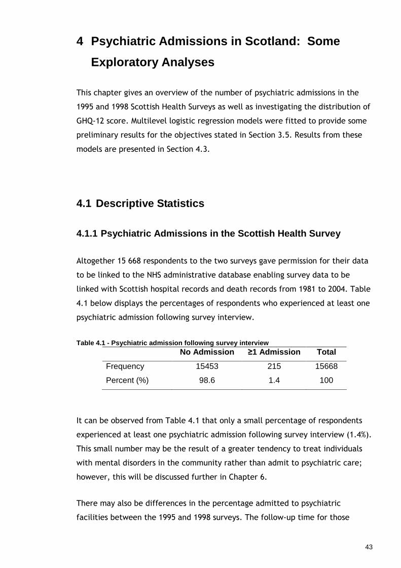
43
4 Psychiatric Admissions in Scotland: Some
Exploratory Analyses
This chapter gives an overview of the number of psychiatric admissions in the
1995 and 1998 Scottish Health Surveys as well as investigating the distribution of
GHQ-12 score. Multilevel logistic regression models were fitted to provide some
preliminary results for the objectives stated in Section 3.5. Results from these
models are presented in Section 4.3.
4.1 Descriptive Statistics
4.1.1 Psychiatric Admissions in the Scottish Health Survey
Altogether 15 668 respondents to the two surveys gave permission for their data
to be linked to the NHS administrative database enabling survey data to be
linked with Scottish hospital records and death records from 1981 to 2004. Table
4.1 below displays the percentages of respondents who experienced at least one
psychiatric admission following survey interview.
Table 4.1 - Psychiatric admission following survey interview No Admission ≥1 Admission Total
Frequency
Percent (%)
15453
98.6
215
1.4
15668
100
It can be observed from Table 4.1 that only a small percentage of respondents
experienced at least one psychiatric admission following survey interview (1.4%).
This small number may be the result of a greater tendency to treat individuals
with mental disorders in the community rather than admit to psychiatric care;
however, this will be discussed further in Chapter 6.
There may also be differences in the percentage admitted to psychiatric
facilities between the 1995 and 1998 surveys. The follow-up time for those

Chapter 4
44
interviewed in the 1995 survey was longer, perhaps implying that a greater
percentage of admissions is to be expected. Table 4.2 investigates this.
Table 4.2 - Psychiatric admission following survey interview by survey year 1995 Survey 1998 Survey Total No Admission Frequency Percent (%)
7246 98.4
8207 98.8
15453 98.6
≥1 Admission Frequency Percent (%)
117 1.6
98 1.2
215 1.4
Total Frequency Percent (%)
7363 100
8305 100
15668
100
Table 4.2 shows that there was a slightly higher percentage of admissions during
follow-up for those who were interviewed in 1995 than in 1998 (difference of
0.4%). This may be as expected as a result of the longer follow-up period for
respondents of the 1995 survey. The difference could also be due to differences
in the age distributions between the two surveys. Recall that the 1995 survey
was restricted to those under 65 years, whereas the 1998 survey was restricted
to those under 75 years. If younger individuals are at a greater risk of admission,
then a higher percentage of admissions may again be expected in the 1995
survey.
Stewart [30] reported differences in the likelihood of psychiatric admission
depending on whether or not an individual had experienced at least one previous
psychiatric admission. Using single-level logistic regression on the 1995 and 1998
linked SHeS dataset, Stewart found that those with at least one previous
psychiatric admission had highly significantly greater odds (OR = 30.3, 95% CI =
(22.4, 41.0)) of being admitted to psychiatric facilities following survey
interview than those with no known history of psychiatric admission prior to
survey interview. This result suggests it may be sensible to stratify analyses
according to whether or not a respondent has a known history of psychiatric
admission. This will mean that risk factors for first psychiatric admission and for
readmission can be investigated separately. Table 4.3 below shows the
percentage of subjects admitted to psychiatric facilities by type of admission,
i.e. first admission if the respondent had no known history of psychiatric

Chapter 4
45
admission prior to survey interview or readmission if the respondent had at least
one psychiatric admission prior to survey interview. To recap, the rows of the
table correspond to admissions following survey interview, and the columns of
the table correspond to admissions prior to survey interview.
Table 4.3 - Psychiatric admission following survey interview by number of prior admissions No Prior
Admission ≥1 Prior
Admission
Total No Admission Frequency Percent (%)
15168 99.1
285 78.5
15453 98.6
≥1 Admission Frequency Percent (%)
137 0.9
78
21.5
215 1.4
Total Frequency Percent (%)
15305 100
363 100
15668
100
After omitting those with prior admission(s) there were 15305 respondents with
no known history of psychiatric admission prior to survey interview, and of them
only a small percentage was admitted to psychiatric facilities following survey
interview (0.9%). Of the 363 respondents with history of at least one psychiatric
admission prior to survey interview, 21.5% went on to be readmitted following
survey interview. When considering first admissions and readmissions separately,
Table 4.3 also reveals that the number of respondents who had at least one
psychiatric admission prior to survey interview is very small (= 363). This is only
2.3% of the original 15668 respondents for whom data were available. Because of
this small number of respondents, analyses will focus solely on investigating the
association between GHQ-12 score and psychiatric admission for those with no
known history of psychiatric admission prior to survey interview (i.e.
respondents for whom any admission following survey interview is assumed to be
a first-ever admission).
4.1.2 Distribution of GHQ-12 Score in the Scottish Health Survey
Each respondent in the SHeS had data recorded on actual GHQ-12 score (i.e. an
integer-valued score between 0 and 12). However, rather than use the ordinal

Chapter 4
46
version, GHQ-12 score was categorised into four categories corresponding to
whether the respondent had a score of 0, 1-2, 3-4 or 5-12. Categories were
defined in this way in order to distinguish between those with no or low risk of
psychiatric caseness (i.e. a score of 0), those with a borderline risk of psychiatric
caseness (i.e. a score of 1-2 or 3-4 depending on the threshold score employed)
and those with a high risk of psychiatric caseness (i.e. a score of 5-12). Table
4.4 displays the distribution of GHQ-12 score in the SHeS.
Table 4.4 - Distribution of GHQ-12 score in SHeS Score 0 Score 1-2 Score 3-4 Score 5-12 Total
Frequency
Percent (%)
8771
57.3
3232
21.1
1331
8.7
1971
12.9
15305
100
The majority of respondents in the SHeS had a GHQ-12 score of 0 (57.3%), and
would therefore be considered as being at low risk of psychiatric caseness,
which, using these data, is being represented by having no admission to
psychiatric facilities. Only 12.9% of respondents obtained a GHQ-12 score in the
high risk category (a score of 5-12).
It is also of interest to check for any trend in the percentage of respondents
admitted to psychiatric facilities across GHQ-12 score in order to informally
investigate the association between GHQ-12 score and psychiatric admission,
which is the primary objective using the SHeS data.
Table 4.5 - Psychiatric admission following survey interview by GHQ-12 score Score 0 Score 1-2 Score 3-4 Score 5-12 Total No Admission Frequency Percent (%)
8725 99.5
3198 98.9
1313 98.6
1932 98.0
15168 99.1
≥1 Admission Frequency Percent (%)
46 0.5
34 1.1
18 1.4
39 2.0
137 0.9
Total Frequency Percent (%)
8771 100
3232 100
1331 100
1971 100
15305 100
Table 4.5 demonstrates that, informally, psychiatric admission following survey
interview appears to be associated with GHQ-12 score. The percentage of

Chapter 4
47
respondents experiencing at least one psychiatric admission following survey
interview increased as GHQ-12 score increased, indicating a possible increasing
trend. This trend will be investigated formally in Section 4.3 of this chapter and
in later chapters.
4.1.3 Missing Data in the Scottish Health Survey
Of the 15305 individuals with no known of history psychiatric admission prior to
survey interview, 1584 (10.3%) had missing data on at least one variable. Two
primary consequences of ignoring missing data include loss of power and biased
estimates of associations [144]. Although the proportion of missing data in the
SHeS was small, it was still of interest to impute values for the missing data
since it is known that, even when the proportion of missing data is small,
potential bias can still occur [145, 146].
Missing data were imputed in SPSS 14.0 [147] using the missing value analysis
regression technique. This method involved treating variables with missing
values as dependent variables to be predicted by the other variables in the
dataset using multiple linear regression. As this produced continuous estimates
for the imputed values, the imputed values obtained for categorical variables
were rounded to the nearest whole category. It is accepted that other more
sophisticated methods of imputation are available for this purpose, and these
will be considered in the Discussion (Chapter 10). However, as the purpose of
this thesis was not focused on estimating missing values, and also due to time
constraints, only the multiple regression method described here was used.
When imputing missing data in SPSS using the missing value analysis regression
technique, a random component can be added to the regression estimates to
reflect the uncertainty associated with the imputation [148]. The random
component selected can either be residuals, normal variates or Student’s t
variates. Alternatively, no adjustment can made.

Chapter 4
48
4.2 Applying Multilevel Modelling to Logistic Regre ssion
In health research, it is common to observe outcomes that are not measured on
a continuous scale. For example, some health outcome data are qualitative, and
in particular binary. In that case there are two possible outcomes (of which only
one can occur), such as ‘alive/dead’ or ‘pass/fail’. In general, these can be
referred to as ‘response’ or ‘non-response’ depending on the outcome of
interest.
Linear regression cannot be used sensibly to model these outcomes on a set of
explanatory variables. Instead, so-called generalised linear models are applied in
which there exists a linear predictor based on the explanatory variables
η = ∑xPβP ,
where the coefficients β1, . . . , βq are unknown.
In the case of binary data, the objective is to measure the response probability,
π, based on a set of explanatory variables. A suitable link function, g, maps the
response onto the predictor such that
g(πi) = ηi = ∑xiPβP ,
for the ith unit (i = 1, . . . , n). There are a number of link functions available to
do this. Only the logit/logistic function will be discussed here; however, a full
discussion of other possible link functions is given in McCullagh and Nelder [149].
The logit/logistic function is of the form
g(π) = log[π/(1- π)] = logit(π).
The logit link function allows values of g(π), or logit(π), to take any value in the
range (-∞, ∞) by transforming the original probability values which are bounded
between 0 and 1, whilst ensuring that predicted probabilities derived from the
fitted model are in the range [0,1] [150]. Some reasons why the logit/logistic
function is favoured over alternative link functions are that it has simpler

Chapter 4
49
theoretical properties and the coefficients from a logit model can be interpreted
simply as logarithms of odds ratios (or as odds ratios when exponentiated) [149].
For a single-level logistic regression model, yi denotes the binary response for
the ith unit. The observed responses are proportions and follow a binomial
distribution such that
yi ~ Bin(1, πi) ,
where πi is the expected proportion for the ith unit. This is also referred to as a
Bernoulli distribution. The probability of response, i.e. that yi = 1, is denoted by
πi. The single-level logit model can then be written as
logit(πi) = β0 + ∑βpxpi ,
where xpi (p = 1, . . . , q) is the row vector of explanatory variables for the ith
level-1 unit. As discussed previously, the coefficient, βp, from this model is
interpreted as the change in the log odds ratio of a positive response relative to
a negative response for each unit increase in the associated explanatory variable
if the explanatory is continuous; or as the log odds ratio in the case of a
categorical explanatory, where one level of the variable is selected as the
baseline. Exponentiating the right-hand side of this model allows the coefficients
to be interpreted as the odds ratio of a positive response relative to a negative
response for each unit increase in the continuous explanatory variable, or as the
odds ratio when the explanatory is categorical. Rearranging the model allows
the probability of a positive response to be given as
πi = exp(β0 + ∑βpxpi)/[1 + exp(β0 + ∑βpxpi)].
The single-level logistic regression model may be extended to a multilevel model
with two or more levels in order to account for the clustering of binomial
(binary) data nested within higher-level units. The response is given a further
subscript, j, so that yij is the binary response for the ith individual nested within
the jth unit (j = 1, . . . , m). Hence, the probability of response i.e. that yij = 1,
is now denoted by πij.

Chapter 4
50
Following the same form as the single-level model using the logit function, the
multilevel logistic regression model is given as
logit(πij) = log[πij/(1- πij)] = β0 + ∑βpxpij + uj.
As usual, the βp are the coefficients for the fixed effects, xpij; however, in
multilevel random intercept models, the intercept is allowed to vary randomly
across the higher-level unit. uj is the random effect of the higher-level unit.
These higher-level residuals are assumed to follow a Normal distribution with
mean 0 and variance σu2. The full model for estimating probabilities is then
given as
πij = exp(β0 + ∑βpxpij + uj)/[1 + exp(β0 + ∑βpxpij+ uj)].
The coefficients of the explanatory variables are interpreted in the same manner
as in the single-level model. The significance of the fixed effects may be tested
using Wald tests in MLwiN. Testing random parameters, i.e. σu2, is more difficult;
however, a Wald test can provide an approximation. Snidjers and Bosker [151]
provide explanations of alternative methods for testing the random intercept.
When multilevel logistic regression is used, it is also possible to estimate the
intraclass correlation (ICC). Goldstein et al. [152] discussed a number of
procedures for calculating the ICC for discrete response models. In some cases,
they may lead to different answers. In this thesis, all estimates of the ICC for
the logistic regression models in Section 4.3 of this chapter have been calculated
using a procedure called the ‘latent variable approach’ [152]. In this case, the
ICC is estimated as
ICC = σu2/[ σu
2 + π2/3],
where π corresponds to the number pi. For a number of examples to which
multilevel logistic regression could be applied refer to Chapter 3 by Rice on
Binomial Regression in Leyland & Goldstein [153].

Chapter 4
51
4.3 Results from Multilevel Logistic Regression
As discussed in Section 3.5, the primary objective was to investigate the
association between psychological distress, as measured by the GHQ-12, and
first psychiatric hospital admission in Scotland using data from the Scottish
Health Survey, while controlling for a range of risk factors. This section presents
results obtained from fitting multilevel logistic regression models in MLwiN.
Multilevel models were fitted in order to account for the hierarchical structure
of the data which consisted of two levels – individuals nested within postcode
sectors. The binary response was of the form ‘subject did or did not experience
a psychiatric admission following survey interview’. Results presented in this
section are for those respondents with no psychiatric admissions prior to survey
interview (see Section 4.1 for a further discussion of this). Results from the
multilevel logistic regression models will give a prior insight into results to be
expected from fitting the more complex multilevel event history models.
A binomial model with logit link was fitted to the imputed dataset including the
random component (residual), and the parameter estimates were obtained using
first-order penalised quasi-likelihood (PQL) estimation (see Section 5.3.5 for a
discussion of estimation procedures). First-order PQL was used as parameter
estimates would not converge when 2nd-order PQL was used. The outcome was
assumed to be binomially distributed.
In Section 4.1, Table 4.5 showed that, subjectively, there appeared to be an
increase in the percentage of respondents admitted to psychiatric facilities
following survey interview as GHQ-12 score increased. To investigate if this
increase was significant model A1, containing GHQ-12 score and a random
intercept for postcode sector, was fitted.
Following the fitting of only GHQ-12 score in model A1, it was then of interest to
investigate if the association between increasing GHQ-12 score and increased
odds of psychiatric admission remained after adjustment for a range of
individual- and area-level demographic, socioeconomic and lifestyle risk factors.
As discussed in Section 3.2.1.2, GHQ-12 score is highly correlated with self-
assessed general health in predicting mental health outcomes. Therefore, in

Chapter 4
52
order to avoid potential over-controlling if both of these variables were included
in the model, models were fitted both including and excluding self-assessed
general health. Model A2 fitted all individual- and area-level risk factors apart
from self-assessed general health, and finally, model A3 was fitted as in model
A2 but including self-assessed general health. In order to investigate how much
of the variation in the odds of psychiatric admission between postcode sectors
could be explained by individual characteristics, models A2 and A3 were at first
fitted allowing only for the adjustment of individual-level risk factors. After
removal of all non-significant individual-level risk factors, area-level risk factors
(which included a measure of deprivation and a measure of urbanicity) were
added to the models. The remaining variation in the odds of psychiatric
admission between postcode sectors explained by adding these variables could
then be calculated.
Both estimates of the fixed and random parameters and estimated standard
errors obtained from fitting the three separate models are presented in Table
4.6 below. Due to the large number of variables that were available in this
dataset, Table 4.6 displays results for significant individual- and area-level risk
factors only. Table 2.1 provides a comprehensive list of all available risk factors.
Results from model A1 demonstrated that there was a highly significant
increasing trend in the odds of first psychiatric admission during follow-up as
GHQ-12 score increased. It can also be observed that the odds of psychiatric
admission for each category of GHQ-12 score were significantly different from
that of the baseline score of 0. This indicated that any GHQ-12 score of 1 or
more is significantly associated with psychiatric admission, implying that a score
of 1 may be a suitable threshold score for the GHQ-12 in the Scottish population.
After adjustment for GHQ-12 score, the probability of psychiatric admission in
the average area for an individual with a GHQ-12 score of 0, obtained by taking
the antilogit function of the intercept, was 0.0052. The intra-class correlation
(ICC) indicated that 7.9% of the total variation was due to differences between
postcode sectors.

Chapter 4
53
Table 4.6 - Results from multilevel logistic regres sion Model A1 Model A2 Model A3 Estimate(s.e) Estimate(s.e) Estimate(s.e) Fixed
Intercept (β0) -5.253(0.150) -5.731(0.310) -5.940(0.327)
GHQ-12 Score 0 0.000** 0.000** 0.000* 1-2 (β1) 0.701(0.227) 0.580(0.229) 0.485(0.231) 3-4 (β2) 0.959(0.280) 0.670(0.285) 0.512(0.290) 5-12 (β3) 1.342(0.220) 0.930(0.229) 0.671(0.239)
Sex Male 0.000 0.000 Female (β4) -0.137(0.189) -0.088(0.190)
Age 16-24 0.000 0.000 25-34 (β5) -0.287(0.289) -0.254(0.291) 35-44 (β6) -0.012(0.280) 0.028(0.283) 45-54 (β7) -0.682(0.336) -0.737(0.339) 55-64 (β8) -0.277(0.307) -0.397(0.312) 65-74 (β9) -0.112(0.387) -0.082(0.389)
Marital Status Married/cohabiting 0.000 0.000 Other (β10) 0.534(0.180) 0.439(0.183)
Receipts of Benefits No 0.000 0.000 Yes (β11) 0.781(0.202) 0.567(0.211)
Smoking Status Non-Smoker 0.000 0.000 Current Smoker (β12) 0.794(0.215) 0.697(0.217) Ex-Smoker (β13) 0.028(0.302) -0.002(0.303)
Employment Status Full-Time 0.000 0.000 Unemployed (β14) 0.445(0.267) 0.573(0.272) Part-Time (β15) -0.353(0.255) -0.303(0.256)
Self-Assessed Health Very Good 0.000 Good (β16) 0.566(0.226) Fair (β17) 1.040(0.252) Bad (β18) 0.319(0.558) Very Bad (β19) 2.076(0.472)
Random
Area Variation(σu2) 0.281(0.268) 0.220(0.257) 0.239(0.255)
ICC 0.079 0.063 0.068 * ptrend < 0.05 ** ptrend <0.001
Chapter 4
54
Model A2 displays results obtained following adjustment for all significant
individual-level risk factors excluding self-assessed general health. The
increasing trend in the odds of psychiatric admission remained highly significant,
and, in addition to having a GHQ-12 score of 1 or more, other significant risk
factors associated with an increased odds of psychiatric admission included not
being married (i.e. single, separated, divorced or widowed), being in receipt of
benefits and finally, being a current smoker. Again this indicated that, even
following adjustment for a range of other risk factors, a score of 1 appears to be
a suitable threshold score for the GHQ-12 in the Scottish population. The
between-postcode sector variation (σu2 = 0.220) was reduced from model A1 to
model A2, with approximately 22% of the total unexplained variation between
postcode sectors being explained as a result of adjusting for further individual-
level risk factors. Neither of the area-level risk factors was significantly
associated with the outcome in addition to the individual-level risk factors.
In fitting model A3, self-assessed general health was also allowed to be included
as a potential risk factor. The increasing trend in the odds of outcome remained
significant following adjustment for all significant individual-level risk factors, of
which those associated with an increased odds of psychiatric admission, in
addition to a GHQ-12 score of 1 or more, included the following: not being
married (i.e. single, separated, divorced or widowed); being in receipt of
benefits; being a current smoker; being unemployed; and having a self-assessed
general health rating of other than ‘very good’. As with the two previous
models, this model demonstrated that, even after adjustment for a range of
other risk factors, this time including self-assessed general health, a GHQ-12
score of 1 appeared to be an appropriate threshold score in the Scottish
population. Again, neither of the area-level risk factors was associated with the
outcome when added to the model including all the significant individual-level
risk factors. The between-postcode sector variation in model A3 (σu2 = 0.239)
increased from model A2 as a result of including self-assessed general health. An
explanation of this phenomenon can be found in Snijders and Bosker [151].

Chapter 4
55
4.4 Chapter Summary
Fitting multilevel logistic regression models has given an insight into individual-
level and area-level risk factors associated with first psychiatric admission in
Scotland, while acknowledging the hierarchical structure of the data. However,
as the data were from the 1995 and 1998 Scottish Health Surveys, the lengths of
follow-up times from survey interview until 2004 were different for the two
surveys. A more appropriate approach, which would account for differences in
follow-up times between the two surveys, is to use multilevel event history
models. One of the main differences in using event history analysis methodology
over logistic regression is that time until the event of interest can be partially
observed. In this case, for subjects who experience a psychiatric admission after
survey interview, the time variable records the actual time to event. However,
for subjects who do not experience a psychiatric admission, the time variable
refers to length of follow-up. This is an incomplete observation of survival time,
and these incomplete observations are referred to as being ‘censored’. In this
study, observations will be censored if the subject dies or reaches the end of
follow up without experiencing a psychiatric admission (or if they are lost to
follow-up). Event history models are particularly important when the length of
follow-up is long, and therefore the number of individuals dying or being lost to
follow-up may be large. Additionally, it has been shown in previous literature
that psychological distress, as measured by the GHQ, is associated with a higher
risk of mortality [154, 155]. Since results from the multilevel logistic regression
in Table 4.6 showed that those with a higher GHQ score were at a greater risk of
psychiatric admission, based on the previous literature this would also imply that
individuals with an increased risk of psychiatric admission are at greater risk of
death, and hence censoring. Once again this demonstrates that the use of
multilevel event history models is preferred over multilevel logistic regression.

56
5 Multilevel Event History Modelling: A Review
5.1 Introduction
This chapter will provide a review of conventional methods used for fitting
multilevel event history models to public health data. It will discuss problems
which may be encountered when datasets are large, as is usually the case with
public health survey data. Successive chapters review possible methods which
could be used to overcome these problems.
Event history models are also commonly referred to as ‘survival models’ in the
context of biology and health. Since this thesis is concerned with the application
of event history models to public health research, such models will now be
referred to as ‘survival models’ in the text.
5.2 Single-Level Survival Modelling
5.2.1 Introduction to Survival Modelling
When analysing medical or public health datasets, it may often be of interest to
measure the time until a particular pre-defined event occurs, such as death from
a particular disease. This time is known as the survival time. With the SHeS
dataset, interest was in observing the time until first psychiatric hospital
admission as measured from survey interview, and the effect that demographic,
socioeconomic and lifestyle risk factors had on the survival time. If time until
event, i.e. the survival time, is treated as a continuous variable, it may seem
reasonable to regress the natural logarithm of time on the covariates; however,
as discussed in Allison [156] and Petersen [157], there are two problems with
this approach. Firstly, there may be some individuals who do not experience the
event of interest during the period of follow-up. For example, when following-up
individuals in the SHeS data to measure time until first psychiatric hospital
admission, it is highly likely that not all individuals will experience a psychiatric
hospital admission during the follow-up period. These individuals are referred to
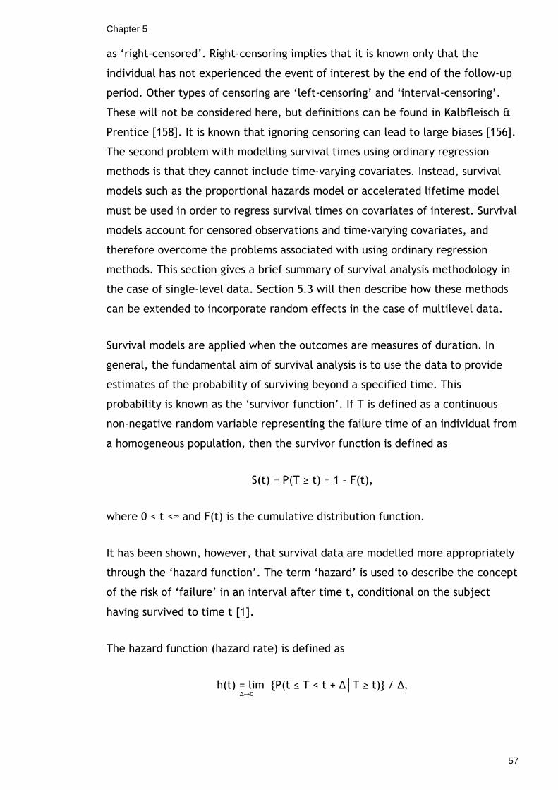
Chapter 5
57
as ‘right-censored’. Right-censoring implies that it is known only that the
individual has not experienced the event of interest by the end of the follow-up
period. Other types of censoring are ‘left-censoring’ and ‘interval-censoring’.
These will not be considered here, but definitions can be found in Kalbfleisch &
Prentice [158]. It is known that ignoring censoring can lead to large biases [156].
The second problem with modelling survival times using ordinary regression
methods is that they cannot include time-varying covariates. Instead, survival
models such as the proportional hazards model or accelerated lifetime model
must be used in order to regress survival times on covariates of interest. Survival
models account for censored observations and time-varying covariates, and
therefore overcome the problems associated with using ordinary regression
methods. This section gives a brief summary of survival analysis methodology in
the case of single-level data. Section 5.3 will then describe how these methods
can be extended to incorporate random effects in the case of multilevel data.
Survival models are applied when the outcomes are measures of duration. In
general, the fundamental aim of survival analysis is to use the data to provide
estimates of the probability of surviving beyond a specified time. This
probability is known as the ‘survivor function’. If T is defined as a continuous
non-negative random variable representing the failure time of an individual from
a homogeneous population, then the survivor function is defined as
S(t) = P(T ≥ t) = 1 – F(t),
where 0 < t <∞ and F(t) is the cumulative distribution function.
It has been shown, however, that survival data are modelled more appropriately
through the ‘hazard function’. The term ‘hazard’ is used to describe the concept
of the risk of ‘failure’ in an interval after time t, conditional on the subject
having survived to time t [1].
The hazard function (hazard rate) is defined as
h(t) = lim P(t ≤ T < t + ∆T ≥ t) / ∆, ∆→0

Chapter 5
58
and specifies the instantaneous rate of failure. The hazard function can also be
defined in terms of the survivor function so that
h(t) = f(t)/S(t),
where f(t) is the probability density function.
The survivor and hazard functions may be estimated parametrically by fitting
any non-negative distribution to describe the survival data. They may also be
estimated non-parametrically, for example, using the Kaplan-Meier estimator.
The most common parametric distributions for describing survival data include
the exponential, Weibull, log-normal, gamma and so on. These will not be
discussed in detail here; however, a review of the most commonly used
parametric distributions can be found in books by Cox & Oakes [159], Klein &
Moeschberger [160], Hougaard [161] and Kalbfleisch and Prentice [158]. Choice
of parametric distribution depends on a number of different factors, for
example, the type of survival data (e.g. human lifetimes) and their convenience
for statistical inference. Cox & Oakes [159] and Hougaard [161] provide
comparisons of parametric distributions used for describing survival data based
on, among others, properties of the hazard and the number of parameters in the
distribution. However, as discussed above, it is possible to avoid assuming a
particular parametric distribution altogether by using non-parametric methods.
Common non-parametric methods for estimating the survivor function in the
presence of right-censoring include the Kaplan-Meier estimator, also known as
the Product-Limit estimator, and the Nelson-Aalen estimator. Again, these will
not be covered here, but full definitions of these estimators can be found in
Hougaard [161] and Kalbfleisch & Prentice [158]. A clear disadvantage of the
non-parametric methods is that estimation of the hazard function is not possible
therefore, if interest lies more in estimating the hazard function rather than the
survivor function, parametric methods should be used. For further comparisons
of parametric and non-parametric methods refer to Hougaard [161].
With survival data, there may also be information available on a number of
explanatory variables or covariates, which may have an effect on failure time.
The most commonly used models are the proportional hazards and accelerated
lifetime models. Both will now be considered.

Chapter 5
59
5.2.2 Proportional Hazards Model
If h(t, x) is the hazard function at time t for an individual with covariate vector
x, then the proportional hazards model (PHM) is defined as
h(t;x) = h0(t)exp(βTx) ,
Equation 5.1
where h0(t) is a baseline hazard function (i.e. the hazard for an individual with
x=0), and β is a vector of unknown regression parameters. The survivor function
is thus given as
( )[ ] ( )xT
tSxtTPxtS βexp0)();( =>= ,
where S0(t) is the baseline survivor function, and can be written in terms of the
baseline hazard function, h0(t), as follows:
S0(t) = exp- ∫t
0
h0(u) du .
The baseline hazard function, h0(t), could assume some parametric form. More
commonly, however, the form of the baseline hazard is left unspecified yielding
the widely-used semi-parametric (Cox) PHM. This model is semi-parametric in
the sense that a parametric form is assumed only for the covariate effect, with
the baseline hazard function treated non-parametrically. When the model is
semi-parametric, the method of analysis for estimation of the β regression
parameters is partial likelihood, with the hazard function being treated as a
nuisance parameter. If it is assumed that censoring is non-informative right-
censoring, this method is based on the conditional probability that individual i
experiences the event in the next unit of time, ti+δti , given that only one
individual from the risk set (Ri, i.e. the set of individuals at risk at time ti) fails
at that time.

Chapter 5
60
Therefore, supposing that there are no tied observations, under the PHM this
conditional probability can be written as
( ) ( )( ) ( )∑
∈ iRjj
Ti
T
xth
xth
ββ
exp
exp
0
0 .
This expression simplifies since the baseline hazard function, h0(t), cancels out,
therefore, the partial likelihood for β is
( ) ( )( )∏
∑=∈
=m
iRj
jT
iT
i
x
xL
1 exp
exp
βββ .
for m distinct failure times. There are various ways in which the partial
likelihood can be modified when there are tied observations among the
uncensored failure times. These will not be considered here, but a full
explanation can be found in Klein & Moeschberger [160] and Kalbfleisch and
Prentice [158].
Although the β regression parameters may be estimated using the partial
likelihood as described above, it may also be of interest to estimate the survivor
function for any set of values of the covariates. There are a number of ways this
can be done non-parametrically, and, although they will not be covered here, a
review can be found in Kalbfleisch & Prentice [158].
In some cases, there may be information on covariates whose values change over
the course of the study, i.e. time-varying covariates. The PHM can easily be
extended to incorporate time-varying covariates. Information on this can be
found in Klein & Moeschberger [160].

Chapter 5
61
5.2.3 Accelerated Lifetime Model
Although perhaps not as widely used as the proportional hazards model, the
accelerated lifetime model is, however, another commonly used model in
survival regression analysis. The hazard function for duration in the accelerated
lifetime model is defined as
h(t; x) = h0t exp(βTx)exp(βTx) ,
Equation 5.2
where h0 is the baseline function, and x is the covariate vector. From this it is
clear that the explanatory variables have a direct effect on the survival time,
and accelerate or decelerate the time to failure [162]. This effect makes
interpretation of results clearer in the accelerated lifetime model, where results
refer to the effect of covariates on the mean survival time; rather than in the
PHM, where instead results refer to the effects of covariates on a conditional
probability [162]. As well as the fact that interpretation of results is generally
simpler using the accelerated lifetime model, another reason why it may be
preferred over the PHM is that it does not require the assumption of proportional
hazards. Instead, the accelerated lifetime model assumes proportional
probability of the survival time and the baseline survival i.e. P(T > t x) = P(t0 >
texp(βTx)) [163].
The above function can be written as a log linear model for the random variable
T, modelling the relationship between the (natural) logarithm of survival time
and the covariates such that
ln(T) = α + βTx + σε ,
where α is the intercept and estimate of overall median survival time on the
natural log scale [163], x is the vector of covariates, β is a vector of unknown
regression parameters, σ is an unknown scale parameter, and ε is the random
error term [164] with mean zero and a distribution not depending on x [159].
Examples of distributions for the random error term include the Normal,

Chapter 5
62
Extreme value, Logistic or Gamma distribution. Skrondal & Rabe-Hesketh [165]
discussed examples of accelerated lifetime models depending on the distribution
for the error term - the log-normal duration model if ε is Normally distributed;
the log-logistic duration model for a logistic ε; and the Weibull duration model if
ε follows an extreme value (Gumbel) distribution. The accelerated lifetime
model and proportional hazards model are indeed connected if the extreme
value distribution is used [166] in that the Weibull duration model possesses both
the proportional hazards and accelerated lifetime properties [165]. If the
distribution of the error term is left unspecified, the accelerated lifetime model
may be considered as a semiparametric alternative to the Cox model [158].
Maximum likelihood can be used to estimate the accelerated lifetime model.
Estimation procedures for the accelerated lifetime model will not be considered
here; however, Kalbfleisch & Prentice [158] considered use of the censored data
rank test for estimating the β regression parameters.
As in the proportional hazards model, time-varying covariates may also be
incorporated into the accelerated lifetime model. Information on the inclusion
of time-varying covariates in the accelerated lifetime model can be found in Cox
& Oakes [159] and Kalbfleisch & Prentice [158].
5.3 Multilevel Survival Modelling
5.3.1 Extending the Single-Level Model
This section will briefly describe how single-level survival models may be
extended to incorporate random effects, in particular with reference to the PHM
and accelerated lifetime model. Further details of how these multilevel models
may be fitted using appropriate software is given in Sections 5.3.3 and 5.3.4.
The single-level proportional hazards and accelerated lifetime models may be
extended to incorporate a multilevel structure. As discussed by Goldstein [166],
the multilevel structure of a survival model may arise in two ways. The first
corresponds to when there are repeated durations within individuals, and the

Chapter 5
63
second corresponds to when each individual has a single duration, but the
individuals are grouped within higher-level units. With the SHeS data, interest
lies only in measuring the time until first ever psychiatric admission of
individuals who are nested within postcode-sectors. Therefore, the multilevel
structure when fitting survival models to the SHeS data is a single duration for
each individual with individuals grouped within higher-level units.
Suppose individuals are nested within higher-level units. Then the 2-level
proportional hazards model for the ijth level-1 unit is
h(tij; xij) = h0(tij)exp(βTxij) .
Similarly, the 2-level accelerated lifetime model for the ijth level-1 unit is
hij(t) = h0texp(βTxij)exp(βTxij) .
In the above models, t is a continuous variable, h0 is the baseline hazard function
and xij is the column vector of explanatory variables for the level-1 units.
Explanatory variables may be defined at any level and, as with the single-level
PHM, time-varying covariates, i.e. covariates that vary across failure times, may
be included in the multilevel model. The multilevel PHM and accelerated
lifetime model may be extended to include any number of random effects.
5.3.2 Software for Fitting Multilevel Models
Kelly [167] provided a comprehensive review of six computer packages which
may be used for analysing correlated survival data, namely, SAS, Stata, S-Plus,
R, MLwiN and WinBUGS. In terms of using these packages for fitting multilevel
survival models, the author reviewed them on the basis of the estimation
method used, distributions available for the random effect and user-friendliness.
It was concluded that MLwiN and WinBUGS were the most suitable packages for
fitting survival models with more than one random effect, with MLwiN being the
most suitable when fitting a model to a hierarchical structure and WinBUGS
being preferable if modelling a complex structure. The rest of this chapter

Chapter 5
64
considers the use of MLwiN for fitting multilevel survival models and in
particular, its suitability for fitting multilevel survival models to large datasets.
The use of WinBUGS for fitting such models is considered in Chapter 7.
MLwiN is a package specially designed for fitting multilevel models. The latest
version is MLwiN 2.16, which may be downloaded from
http://www.cmm.bristol.ac.uk/MLwiN/index.shtml. Academics in the UK may
download MLwiN for free.
Although fitting multilevel survival models is not a standard feature of MLwiN,
macros for fitting both the accelerated lifetime and proportional hazards models
are available from the MLwiN website stated above. The use of these macros is
considered in Sections 5.3.3 and 5.3.4. The estimation procedures used in MLwiN
are discussed in Section 5.3.5. A manual for modelling survival data in MLwiN
version 1.20 was written by Yang & Goldstein [163]. This manual is also
appropriate for higher versions of MLwiN.
5.3.3 Fitting a Multilevel Proportional Hazards Mod el in MLwiN
5.3.3.1 Fitting a Multilevel Poisson Model
Both proportional hazards models and accelerated lifetime models (referred to
in MLwiN as a ‘log-duration’ model) can be fitted in MLwiN. This section provides
an overview of how multilevel proportional hazards models can be fitted in
MLwiN. A guide to fitting accelerated lifetime models is provided in Section
5.3.4.
Yang & Goldstein [163] detailed briefly how the multilevel proportional hazards
model for the ijth individual may be fitted in MLwiN using a Poisson model with
log link as follows:
ygij = ln(dgij) ≈ ln(ngij) + ln[(tg+∆-tg)h0(tg)] + βTxij ,

Chapter 5
65
which may be rewritten as
ygij = ln(dgij) ≈ (offset) + φ(tg) + βTxij ,
Equation 5.3
where φ(tg) is a function of time used to model the baseline hazard function.
Possible forms for φ(tg) will be discussed in Section 5.3.3.3. The offset is the
natural logarithm of the number of tied observations, ng. This section gives a
slightly more detailed account of how these expressions are obtained.
Recall from Equation 5.1 that the proportional hazards model at time t for
individual with covariate x is expressed as
h(t;x) = h0(t)exp(βTx) ,
and that the β regression parameters are estimated using the partial likelihood
( ) ( )( )∏
∑=∈
=m
iRj
jT
iT
i
x
xL
1 exp
exp
βββ .
Equation 5.4
Suppose, for each time tg (g = 1 , . . . , h), Yg are independent Poisson random
variables with mean µg, where
µg = mgexp(αg + βTx)
where mg is the total number of individuals at time tg and exp(αg) = (tg+∆-
tg)h0(tg).

Chapter 5
66
For each individual in the risk set at time tg, an artificial Poisson response is
defined such that
Whitehead [168] showed that, when all failure times are distinct, i.e. dgi = 1 at
tg for one individual only and 0 for the rest, the likelihood of the Poisson model
at its maximum is proportional to the maximum of the likelihood in Equation 5.4.
This demonstrates that the estimates of β are identical for the Poisson and
proportional hazards models. Whitehead then went on to describe how the
Poisson model can incorporate tied observations by setting Yg = ng, where ng is
the number of failures at tg (i.e. ng = ∑i dgi), and showed how the likelihood for
this Poisson model at its maximum is proportional to the likelihood for β in
Peto’s generalisation of the proportional hazards model to incorporate ties. This
proves that this Poisson model and Peto’s survival model obtain identical
estimates of β.
Now, it was described by McCullagh & Nelder [149] that because of the
equivalence between the multinomial and Poisson likelihoods, the estimates of β
obtained from the Poisson and multinomial likelihoods are also identical. Thus,
based on the above, the estimate of β obtained from the multinomial likelihood
is identical to that from the partial likelihood for β in Equation 5.4. McCullagh &
Nelder then described that to adjust for tied observations in the multinomial log
likelihood using Peto’s method, the multinomial total should be set to equal the
number of ties at that time (ng, say). This implies that the Poisson log likelihood
is equivalent to Peto’s version of the partial likelihood. Following McCullagh &
Nelder, when adjusting for tied observations, the ‘probabilities’ of the
multinomial response model become
( )( )∑
=
jij
T
ijT
gijgijgij x
xnn
ββ
πexp
exp ,

Chapter 5
67
and therefore the equivalent log-linear model becomes
log(µgij) = log[ngijexp(α + βTxij)]
i.e.
log(µgij) = log[ngijexp(α)exp(βTxij)]
= log[ngij(tg+∆-tg)h0(tg) exp(βTxij)]
= log(ngij) + log[(tg+∆-tg)h0(tg)] + βTxij .
This is equivalent to Equation 5.3.
For the multilevel proportional hazards model, Ma et al. [169] showed how
random effects Poisson models can be used to estimate random effects (Cox)
proportional hazards models. A variance components model for the expected
Poisson count is
πij = exp(αg + βTxij + uj) ,
where αg estimates the baseline hazard function which will be described in
Section 5.3.3.3.
From Equation 5.3, it can be observed that, in order to fit Poisson models, each
duration is expanded so that every individual has a series of records – one for
each time point until either the event of interest or censoring occurs. This
expansion allows the variable dg to be created, where dg is a count of the total
number of failures at time tg. Recall also that the ijth individual will have a
value dgij=0 for each time point they survive, with this becoming dgij=1 if the
individual experiences the event of interest. Therefore, counting up each of the
dgij=1 at a particular time point will give the total number of failures at that
time. This expanded dataset is referred to as a person-period dataset, and will
be discussed further in Section 5.3.3.2.

Chapter 5
68
5.3.3.2 Obtaining the Person-Period Dataset
Section 5.3.3.1 noted that, in order to fit the Poisson model, a person-period
dataset must first be created. This requires each individual’s record to be
replicated as many times as the observed number of time intervals until either
the event of interest or censoring occurs. Clearly, this leads to an expansion in
the size of the original dataset. Using the Scottish Health Survey dataset, this
section will demonstrate how the person-period dataset required to fit the
Poisson model is created in MLwiN.
To fit the Poisson model, MLwiN requires the person-period dataset to include
the following five columns: the response for each individual, dgij; the number of
total failures, dg, at each time tg; a risk time indicator, i.e. an indicator of the
risk set corresponding to each event time; a column of the survival (event) times
and, finally, the number of individuals at the start point of the time. The ‘SURV’
command in MLwiN performs the data expansion to create the expanded dataset
containing the five columns as well as information on available covariates. The
process for expansion of the Scottish Health Survey dataset will now be
considered.
As discussed previously, the dataset is rearranged so that every individual has a
line of data corresponding to each time, tg, until failure or censoring occurs.
Because time is treated as a continuous variable, each tg corresponds to each
distinct event time. Section 4.1.1 noted that, in the SHeS dataset, 137
individuals experienced the event of interest, i.e. admission to psychiatric
facilities. This implies that there should be 137 event times; however, as two
individuals were admitted at the same number of days from survey interview,
there were only 136 distinct event times. Consequently, there were also 136 risk
sets, since a risk set was defined for each distinct failure time, tg.
Consider the SHeS data for the first few individuals in the first postcode sector,
shown below in Table 5.1. Note that, for illustrative purposes, Table 5.1 below
only includes covariate information on GHQ-12 score.

Chapter 5
69
Table 5.1 - Sample of SHeS Data before Expansion
Postcode Sector
Level-1 ID
GHQ-12 Score
Survival Time
Censoring Indicator
(1=censored) 1 1 1 . . .
1 2 3 . . .
1-2 3-4
5-12 . . .
3277 3309 3315
.
.
.
1 1 1 . . .
Following the data expansion, obtained via the ‘SURV’ command in MLwiN, the
person-period dataset for individual 1 in postcode-sector 1 now appears as in
Table 5.2 below.
Table 5.2 - Sample of SHeS Data after Expansion Postcode
Sector Level-1
ID GHQ-12 Score
Response Failure Risk-Time Indicator
Survival Time
Number at Risk
1 1 1 1 1 1 . . 1 1
1 1 1 1 1 1 . . 1 1
1-2 1-2 1-2 1-2 1-2 1-2
.
. 1-2 1-2
0 0 0 0 0 0 . . 0 0
1 1 1 1 1 2 . . 1 1
1 2 3 4 5 6 . .
135 136
20 40 44 51 63 65 . .
2943 3046
15301 15297 15296 15291 15288 15285
.
. 6825 5023
Table 5.2 above contains the five columns created by the ‘SURV’ command in
MLwiN and also any covariate information. The ‘response’ column corresponds to
dgij and, therefore, takes the value 0 for each time point the individual survives
and the value 1 if the individual experiences the event of interest. If and when a
value of 1 is observed, data collection terminates for this individual. The
‘response’ column is the only column from the five created by the ‘SURV’
command that is specific to a particular individual i.e. each individual has their
own response vector, whereas the other four columns correspond to the whole
dataset; therefore, the information in these four columns is replicated for each
individual in the dataset.
From this table it can be observed that the first psychiatric admission (i.e. the
first event) occurred at 20 days from survey interview. As time is being treated
as a continuous variable, this distinct failure time is treated as a risk set. Hence,
in this case, the failure at 20 days from survey interview was the first risk set as
indicated by the ‘risk-time indicator’ column. It can be further observed that

Chapter 5
70
there were 136 risk sets corresponding to each of the 136 distinct failure times.
As discussed above, although there were 137 psychiatric admissions, there were
only 136 distinct failure times since two individuals were admitted at the same
number of days from survey interview. Table 5.2 shows that the ‘tied
observation’ occurred in the 6th risk set which corresponds to a failure time of 65
days. Thus, two individuals were admitted to psychiatric facilities at 65 days as
measured from the date of their respective survey interviews. Recall that tied
observations are accounted for by the offset in the Poisson model, which is the
logarithm of the number of failures at a particular time, tg; hence, in the 6th risk
set, the offset would take the form loge(2).
With respect to the first individual in the first postcode-sector, the expanded
dataset shows that this individual did not experience the event of interest i.e.
they were not admitted to psychiatric facilities at any time during follow-up.
This is clear as the response vector for this individual contains only zeros. It
should also be noted that this individual remained in the study until past the
time of the last psychiatric admission (at which point they were censored). This
is because they have a risk set corresponding to each of the 136 distinct failure
times. If an individual is censored at any point during the study, either as a
result of death or being lost to follow-up, data collection terminates for this
individual; however, their response at time tg of termination would be zero
indicating that termination was a result of censoring and not a result of
experiencing the event of interest.
Creation of the person-period dataset (Table 5.2) led to a vast expansion in the
size of the original dataset (Table 5.1). The person-period dataset contains just
below 1.9 million observations within individuals compared to the original
dataset which contains 15305 individuals.
5.3.3.3 Modelling the Baseline Hazard Function
In Equation 5.3, φ(tg) denoted a function of time used to model the baseline
hazard function. Possible forms for φ(tg) will now be considered. These may
include fitting a polynomial function, using blocking factors, or assuming some

Chapter 5
71
parametric form, such as the Weibull or Exponential distribution. Consider first
the use of blocking factors.
Blocking factors are a set of dummy variables corresponding to the risk sets, and
take the form
α1Z1 + α2Z2 + . . . + αlZl ,
where the α’s are parameters to be estimated and for g = 1, . . . , l;
There may be a dummy variable corresponding to each risk set. Alternatively,
one risk set may be taken as the baseline with the dummy variables then
corresponding to the difference in the baseline log hazard between every other
risk set and the baseline risk set. This implies there will either be tg or tg-1
dummy variables respectively. For the SHeS dataset, when time is being treated
as a continuous variable, recall that there were 136 risk sets. Thus, if using
blocking factors, there would either be 136 or 135 dummy variables. This is a
large number of parameters to be estimated, and therefore this method is not
recommended if there are a large number of risk sets [163]. Indeed, Goldstein
[166] and Yang & Goldstein [163] discussed that, instead of adopting the
blocking factors approach, fitting all of these nuisance parameters may be
avoided by using a polynomial function to obtain efficient estimates of the
model parameters. Yang & Goldstein also noted that the higher the order of the
polynomial, the better the approximation to the baseline hazard and other
estimates in the model. The polynomial function takes the form
α1log(tg) + α2[log(tg)]2 + . . . + αl[log(tg)]
l .
The order of the polynomial should be experimented with until adding further
terms does not alter the model parameters [163].

Chapter 5
72
As discussed above, a parametric form may be assumed for the baseline hazard
function. However, in this thesis, only semiparametric proportional hazards
models will be fitted in MLwiN, and therefore parametric forms will not be
considered here, although Yang & Goldstein [163] briefly described how the
Weibull and Exponential distributions could be fitted in MLwiN to model the
baseline hazard function.
5.3.3.4 Checking the Proportional Hazards Assumptio n
As implied by the name, the so-called ‘proportional hazards’ model requires the
assumption of proportional hazards to hold, otherwise the model can lead to
incorrect inferences [170]. The proportional hazards assumption states that the
relative hazard for the ith individual is proportional in relation to any change of
the covariates [163] i.e. that
( )( ) ( )i
Ti xth
th βexp0
= .
In other words, the ratio of the hazard functions is constant with respect to
time, and hence the hazard functions hi(t) and h0(t) are assumed proportional
[170]. There are a number of possible methods available for assessing the
proportional hazards assumption. A comprehensive review of several methods
can be found in Hess [170]. Yang & Goldstein [163] also described possible
methods which can be used in MLwiN to check the assumption. The method
termed ‘checking the relative hazards’ by Yang & Goldstein will be used for
checking the assumption in this thesis. This method involves including a time-
dependent variable by creating an interaction term between the variable of
interest and the logarithm of time and treating it the same as other time-
independent variables. An non-significant interaction implies that the
proportional hazards assumption is satisfied.

Chapter 5
73
5.3.4 Fitting a Multilevel Accelerated Lifetime Mod el in MLwiN
This section summarises how a multilevel accelerated lifetime model may be
fitted in MLwiN. The notation follows that of Yang & Goldstein [163].
Recall from Equation 5.2 that the form of the general hazard function under the
accelerated lifetime model for the ith individual in the jth level-2 unit at time t is
hij(t) = h0texp(βTxij)exp(βTxij) .
Also, if t0 is an event time from the baseline distribution (i.e. when the values of
the covariates are zero), then, following a natural logarithm transformation, the
accelerated lifetime model with the effects of covariates is
log(Tij) = α + βTxij + uj + log(t0) ,
which may be rewritten as
yij = α + βTxij + uj + eij ,
where uj is the random effect for the jth level-2 unit and follows a Normal
distribution with mean zero and variance σu2. The exponential of the random
effects measures the difference of median survival times among the level-2 units
[163]. Recall that the term for the baseline survival time (t0), eij, can be
assumed to come from a number of different distributions as discussed in Section
5.2.3. Because the dependent variable, yij, is the (natural) logarithm of the
survival time, this model is also referred to as the ‘log-duration’ model [163].
There are a set of macros, named ‘SURVIVAL-V2’, which are used to fit
multilevel log-duration models in MLwiN. Although no data expansion is required
to fit this model (as was required when fitting a proportional hazards model via
a Poisson model), some data preparation is required in order to use the macros.
A brief summary will be provided in this section, but full details can be found in
Yang & Goldstein [163].

Chapter 5
74
The macro requires a distribution to be specified for the error term, eij. MLwiN
allows a choice of four distributions: Normal, Extreme value, Gamma, or
Logistic. Another requirement is that information on the event should be
contained in a column named ‘UNCENS’, taking the value 1 if the ijth individual
experienced the event of interest or 0 if the ijth individual was censored.
5.3.5 Estimation of Parameters in MLwiN
In MLwiN, model parameters are estimated using iterative generalised least
squares (IGLS). However, before this method may be applied for non-linear
models like the Poisson model, discussed in Section 5.3.3.1, quasi-likelihood
methods are used to approximate generalised linear multilevel models by linear
multilevel models. Marginal quasi-likelihood (MQL) and penalised (or predictive)
quasi-likelihood (PQL) are the types of approximation available in MLwiN. This
section will discuss the IGLS algorithm, MQL and PQL as well as the advantages
and disadvantages of using these two approximations. Notation will follow that
of Goldstein [166, 171] and Goldstein & Rasbash [172].
5.3.5.1 Iterative Generalised Least Squares
Consider a linear variance components model with two levels and, for
illustration purposes, just one explanatory variable,
yij = β0 + β1xij + uj + eij .
Suppose the residual covariance matrix, V = cov(YβX), is known. Here, Y is the
response vector and X is the design matrix for the explanatory variable(s), where
Xij is the ijth row of X. Then the estimators for the fixed coefficients can be
obtained using Generalised Least Squares (GLS)
β = (XTV-1X)-1XTV-1Y ,
Equation 5.5

Chapter 5
75
and
cov( β ) = (XTV-1X)-1.
It has been shown by Goldstein [171] that, when the residuals follow a Normal
distribution, Equation 5.5 also generates maximum likelihood estimates. The
iterative estimation procedure starts from reasonable estimates of the fixed
parameters. These are usually obtained from an initial ordinary least squares
(OLS) fit, where it is assumed that σu2 = 0. Here, σu
2 is the variance at level-2.
This yields the OLS estimates of the fixed coefficients, β (0). From this, the
‘raw’ residuals are formed,
y~ ij = yij - β 0 - β 1xij ,
and the vector of raw residuals is written
Y~
= y~ ij .
V is then simply the expected value of the cross-product matrix Y~
Y~ T, i.e.
V = E(Y~
Y~ T) = E(Y*), say .
By stacking the columns of the cross-product matrix it can be rearranged into a
vector, vec(Y*) = Y**, say. A linear model involving the random parameters can
then be written as
E(Y**) = Z*θ ,
where Z* is the design matrix for the random parameters. θ may then be
estimated using GLS
θ = (Z*TV*-1Z*)-1Z*TV*-1Y** ,
Equation 5.6

Chapter 5
76
where
V* = V ⊗ V .
Here, ⊗ is the Kronecker product. The covariance matrix of θ is given as
cov(θ ) = (Z*TV*-1Z*)-1Z*TV*-1cov(Y**)V*-1Z*(Z*TV*-1Z*)-1 .
Goldstein [166] showed that this can be written as
cov(θ ) = 2(Z*TV*-1Z*)-1 .
Using the current estimates of the fixed and random parameters, the IGLS
procedure then iterates between Equations 5.5 and 5.6 [171]. As discussed
previously, starting values for the fixed parameters are usually obtained from an
OLS fit. On achieving convergence, under the assumption of multivariate
Normality, the estimates are maximum likelihood.
5.3.5.2 Restrictive Iterative Generalised Least Squ ares
It is known that, in general, the IGLS procedure produces biased results [166].
This is especially problematic when the sample size is small. Alternatively,
restricted iterative generalised least squares (RIGLS) can be used to obtain
unbiased estimates. These are equivalent to restricted maximum likelihood
estimates (REML) in the multivariate normal case [172]. Instead, E(Y*) = V is
rewritten using the estimates of the fixed parameters, β , to give
E(Y*) = V – Xcov( β )XT = V - X(XTV-1X)-1XT .
From accounting for the sampling variation of β , an unbiased estimate of V is
obtained by adding the second term in the above expression at each iteration
until convergence is obtained. The second term is the ‘hat’ matrix from Y* and
can be considered as a correction for bias [173].

Chapter 5
77
5.3.5.3 Marginal and Penalised Quasi-likelihood
This section refers to Goldstein [166].
Consider a general 2-level model,
yij = X1ijβ1 + Z1ij(2)u1j + Z1ij
(1)e1ij + f(X2ijβ2 + Z2ij(2)u2j + Z2ij
(1)e2ij) + . . . ,
where f is a nonlinear function, X represents the fixed explanatory variables,
Z(1), Z(2) are the random explanatory variables at levels 1 and 2 respectively, and
the ‘+ . . .’ signifies that additional nonlinear functions, involving X or Z(1), Z(2)
terms, may be included in the model. First, a suitable Taylor expansion is used
to linearise the model. This produces a linear model where the explanatory
variables in f are transformed using first and second derivatives of the nonlinear
function.
Goldstein [166] shows that the nonlinear function, f, may be written as the sum
of a fixed-part component and a random part. For the random part, the Taylor
expansion up to a second-order approximation for the ijth unit is given by
fij = fij(Ht+1) + (Z2ij(2)u2j + Z2ij
(1)e2ij)f'ij(Ht) + (Z2ij
(2)u2j + Z2ij(1)e2ij)
2f''ij(Ht)/2 .
Equation 5.7
The first term on the right-hand side of the above expression is the fixed part
value of f at the current ((t+1)th) iteration of the IGLS (or RIGLS) algorithm. The
other two terms are the first and second differentials of the nonlinear function,
which are evaluated at the current values obtained from the previous iteration.
From Equation 5.7 there is
E(Z2ij(2)u2j + Z2ij
(1)e2ij) = 0, E(Z2ij(2)u2j + Z2ij
(1)e2ij)2 = σ2
zu + σ2ze ,
σ2zu = Z2ij
(2)Ωu Z2ij(2)T
, σ2ze = Z2ij
(1)Ωe Z2ij(1)T .

Chapter 5
78
The expansion for the fixed-part value in Equation 5.7 is written as
fij(Ht+1) = fij(Ht) + Xij(β1,t+1 - β1,t) f'ij(Ht) ,
where β1,t+1, β1,t are the current and previous iteration values of the fixed-part
coefficients. Ht may be chosen to be the current value of the fixed-part
predictor, X2ijβ2. This is referred to as a ‘marginal’ quasi-likelihood (MQL) model.
Alternatively, the current estimated residuals may be added when forming the
Taylor expansion to give an improved approximation to the nonlinear component
for each unit. This is referred to as a ‘penalised’ (or ‘predictive’) quasi-
likelihood (PQL) model.
It is known that, in general, the MQL procedure tends to underestimate the
values of the fixed and random parameters. This is especially a problem when
the sample size is small [174, 175]; however, the PQL procedure has been shown
to improve estimates [172]. Greater accuracy may also be obtained by using the
second-order approximation rather than the first-order based upon the first term
in the Taylor expansion. Therefore, improved estimates may be obtained using
the 2nd-order PQL procedure. Intermediate choices include 1st-order PQL and 2nd-
order MQL [150].
5.4 Multilevel Survival Modelling in MLwiN: Result s
5.4.1 Introduction
This section will present results obtained by fitting multilevel survival models in
MLwiN. As discussed previously in Section 3.5, the aim was to investigate the
association between GHQ-12 score and first psychiatric hospital admission in
Scotland, as measured in days from Scottish Health Survey interview. Some
respondents may have had several psychiatric hospital admissions during follow-
up; however, as interest was in modelling time until first psychiatric admission
only, the multilevel structure for the models took the form of a single duration
for each respondent, with respondents being nested within postcode sectors.
Chapter 5
79
This chapter has discussed the use of both the proportional hazards model and
the accelerated lifetime model for investigating the effect of covariates on
survival time. Although the proportional hazards model, estimated using a
Poisson model in MLwiN, is probably the most commonly used survival model,
the use of the accelerated lifetime model may seem more intuitive when fitting
multilevel survival models in MLwiN as it does not require creation of a person-
period dataset. However, Yang & Goldstein [163] discussed that the quasi-
likelihood under IGLS estimation procedure, used by MLwiN to estimate this
model, is prone to breaking down when there are many censored observations.
They suggested that this estimation procedure would not be recommended if
there are more than 50% censored observations in the dataset. Recall that 99.1%
of the observations in the SHeS dataset were censored. Thus, based on the
advice from Yang & Goldstein, a multilevel accelerated lifetime model could not
be fitted in MLwiN. As a result, only proportional hazards models will be used
throughout this thesis when fitting survival models to the SHeS dataset in MLwiN.
To estimate the proportional hazards model, a two-level Poisson model with log
link was fitted in MLwiN and a second-order polynomial was sufficient to smooth
the blocking factors. The polynomial coefficients need not be interpreted since
they are regarded as nuisance parameters. The response is the length of time in
days from Scottish Health Survey interview, and observations were censored if
the subject died or did not experience a psychiatric admission during follow-up.
Note that the results presented in this section are for those respondents with no
psychiatric hospital admissions prior to survey interview. For a further discussion
of this see Sections 3.5 and 4.1.1.
For the continuous-time model, risk sets were defined for each failure time,
which, in this example, was the time in days from survey interview at which a
respondent was admitted to psychiatric facilities. This implied there were 136
risk sets for reasons discussed in Section 5.3.3.2. An offset was fitted in order to
account for any tied observations. This was simply the logarithm of the number
of failures in a particular time interval. In general, the offset was zero, since, as
described above, there was only one interval at which there were tied
observations.

Chapter 5
80
Three separate models were fitted in order to investigate the association
between GHQ-12 score and the hazard of psychiatric admission. Estimates of the
fixed and random parameters with respective estimated standard errors are
displayed in Table 5.3. Parameter estimates were obtained using IGLS and 1st-
order penalised quasi-likelihood (PQL) approximation. IGLS was used as opposed
to RIGLS since the sample size was large (n=15305), and 1st-order PQL was used
rather than the preferred 2nd-order PQL method due to problems with
convergence when trying to use the latter. For a discussion of estimation
procedures see Section 5.3.5. The modelling strategy for the three models will
be described below.
In Section 4.1.2, Table 4.5 showed that, subjectively, there appeared to be an
increase in the percentage of respondents admitted to psychiatric facilities as
GHQ-12 score increased. In order to investigate if this increase was significant,
model B1, containing GHQ-12 score only and a random intercept for postcode
sector, was fitted. Following this, it was then of interest to investigate if the
association between increasing GHQ-12 score and an increased hazard of
psychiatric admission remained after adjustment for a range of individual- and
area-level demographic, socioeconomic and lifestyle risk factors.
As discussed in Section 3.2.1.2, GHQ-12 score is highly correlated with self-
assessed general health in predicting mental health outcomes and therefore, in
order to avoid potential over-controlling models were fitted both including and
excluding self-assessed general health. Model B2 fitted all individual- and area-
level risk factors apart from self-assessed general health and, finally, model B3
was fitted as in Model B2 but including self-assessed general health.
In order to investigate how much of the variation in the hazard of psychiatric
admission between postcode sectors could be explained by individual
characteristics, models B2 and B3 were at first fitted allowing only for the
adjustment of individual-level risk factors. After removal of all non-significant
individual-level risk factors, area-level risk factors (which included a measure of
deprivation and a measure of urbanicity) were then added to the models. This
allowed calculation of how much of the remaining variation in the hazard of
psychiatric admission between postcode sectors was explained by these variables

Chapter 5
81
when added to the models with all significant individual-level risk factors
included.
Due to the large number of variables available in this dataset, Table 5.3 only
displays results for significant individual- and area-level risk factors only. Table
2.1 provides a comprehensive list of all available risk factors.
5.4.2 Results from Multilevel Continuous-Time Hazar d Model
Results from fitting the multilevel continuous-time hazard model via a Poisson
model in MLwiN are given in Table 5.3. Results from checking the proportional
hazards assumption are given in Appendix 2.
Results from model B1 concluded that there was a highly significant increasing
trend in the hazard of psychiatric admission (p < 0.001) as GHQ-12 score
increased. The between-postcode sector variation (σu2 = 0.255) was large in
comparison to the average hazard of psychiatric admission (for a person with a
GHQ-12 score of 0) when accounting for GHQ-12 score (exp(β0) = 0.00004). The
large between-postcode sector variation implied a greater similarity in the
hazard of event for individuals within a postcode sector. Parameter estimates
for the log hazard ratios in model B1 were similar to those for the log odds ratios
in model A1 (Table 4.6). This is not unexpected, since it has been shown that the
proportional hazards model and logistic regression model yield similar results
when the outcome of interest is rare, in particular less than 5% [176]. Recall that
0.9% of individuals experienced the outcome of interest in this dataset.

Chapter 5
82
Table 5.3 - Results from multilevel continuous-time hazard model Model B1 Model B2 Model B3 Estimate(s.e) Estimate(s.e) Estimate(s.e) Fixed
Intercept (β0) -10.173(0.165) -10.684(0.317) -10.866(0.333)
Log(tij) (α1) 0.227(0.117) 0.227(0.117) 0.203(0.116)
Log(tij)^2 (α2) 0.089(0.061) 0.087(0.061) 0.076(0.061)
GHQ-12 Score 0 0.000** 0.000** 0.000* 1-2 (β1) 0.699(0.226) 0.571(0.228) 0.483(0.229) 3-4 (β2) 0.964(0.278) 0.676(0.282) 0.535(0.286) 5-12 (β3) 1.353(0.218) 0.944(0.227) 0.713(0.236)
Sex Male 0.000 0.000 Female (β4) -0.146(0.187) -0.107(0.187)
Age 16-24 0.000 0.000 25-34 (β5) -0.274(0.286) -0.245(0.287) 35-44 (β6) 0.009(0.277) 0.048(0.279) 45-54 (β7) -0.636(0.333) -0.687(0.335) 55-64 (β8) -0.196(0.304) -0.302(0.308) 65-74 (β9) 0.161(0.384) 0.207(0.386)
Marital Status Married/cohabiting 0.000 0.000 Other (β10) 0.474(0.179) 0.390(0.181)
Receipts of Benefits No 0.000 0.000 Yes (β11) 0.801(0.200) 0.605(0.210)
Smoking Status Non-Smoker 0.000 0.000 Current Smoker (β12) 0.812(0.213) 0.722(0.215) Ex-Smoker (β13) 0.035(0.300) 0.016(0.301)
Employment Status Full-Time 0.000 0.000 Unemployed (β14) 0.425(0.262) 0.541(0.267) Part-Time (β15) -0.365(0.253) -0.317(0.254)
Self-Assessed Health Very Good 0.000 Good (β16) 0.505(0.225) Fair (β17) 0.962(0.249) Bad (β18) 0.191(0.553) Very Bad (β19) 1.917(0.456) Random Area Variation(σu
2) 0.255(0.263) 0.201(0.250) 0.246(0.247)

Chapter 5
83
* ptrend < 0.05 ** ptrend <0.001
Following adjustment for all significant individual-level risk factors, apart from
self-assessed general health, results from model B2 revealed that any GHQ-12
score of 1 or more remained significantly associated with an increased hazard of
psychiatric admission (p = 0.005). The increasing trend continued to be highly
significant (p < 0.001). In addition to having a GHQ-12 score of 1 or more, other
significant individual-level risk factors associated with an increased hazard of
psychiatric admission included not being married (i.e. single, separated,
divorced or widowed), being in receipt of benefits and finally, being a current
smoker. When added to the model including all significant individual-level risk
factors, neither of the area-level risk factors was significantly associated with
the outcome, and hence their addition did not explain any of the remaining
variation between postcode sectors. Thus, the final version of model B2
contained (significant) individual-level risk factors only. The between-postcode
sector variation in model B2 (σu2 = 0.201) reduced from model B1 as a result of
adjusting for further risk factors, with approximately 21% of the total
unexplained variation between postcode sectors being explained as a result of
going from model B1 to model B2.
Finally, following adjustment of all significant individual-level risk factors as
well as self-assessed general health, results from model B3 indicated that,
although the effect of GHQ-12 score on the hazard of psychiatric admission was
attenuated when self-assessed general health was included, the increasing trend
in GHQ-12 score remained significant (p = 0.002). Results from model B3
indicated that, in addition to a GHQ-12 score of 1 to 2 or 5 to 12, other
significant individual-level risk factors associated with an increased hazard of
admission included not being married (i.e. single, separated, divorced or
widowed), being in receipt of benefits, being a current smoker, being
unemployed, and having a self-assessed general health rating of other than ‘very
good’. Again, when the two area-level risk factors were added to the model
containing all significant individual-level risk factors, neither was significantly
associated with the outcome. Therefore, the final version of model B3 contained
(significant) individual-level risk factors only. Just as in model A3 when logistic

Chapter 5
84
regression was used, the between-postcode sector variation in model B3 (σu2 =
0.246) increased from model B2 as a result of including self-assessed general
health.
The possibility of over-controlling, if self-assessed general health was included in
the model in addition to GHQ-12 score, was discussed earlier in this section and
also more extensively in Section 3.2.1.2. Results from model B3, however, have
shown that the increasing trend in the hazard of psychiatric admission still
remained significant (p = 0.002) after inclusion of self-assessed general health.
This suggested that both measures, in addition to each other, were still related
to the outcome. Self-assessed general health was more strongly related to the
outcome and therefore, if only one measure of potential psychiatric morbidity
were available, this may be the better option. However, even after adjustment
for self-assessed general health, GHQ-12 score still provided some information,
implying that the two measures, used in combination with each other, were
more powerful at prediction.
5.4.3 Summary
As discussed throughout this chapter, when fitting the continuous-time survival
models to the SHeS data (with corresponding results displayed in Table 5.3), risk
sets were defined for each failure time, which was the time in days from survey
interview at which a respondent was admitted to psychiatric facilities. This
discussion demonstrated that, in order to fit the Poisson models, the data had to
be rearranged into a suitable form as shown in Table 5.2. Rearranging the data
into this format meant that each respondent then had a line of data
corresponding to each risk set they survived, and hence the size of the dataset
expanded from 15305 respondents to just less than 1.9 million data points within
respondents.
Defining risk sets for each failure time was not particularly problematic for the
Scottish Health Survey dataset as its size (n=15305) was not exceptionally large.
However, when considering much larger datasets, defining risk sets in this way
may prove to be much more troublesome since, when rearranged, the expanded

Chapter 5
85
person-period dataset will also be much larger. Larger datasets may lead to
computational problems, either when trying to expand the data to create the
person-period dataset in order to fit the Poisson models, or when trying to
estimate the models in MLwiN. Therefore, alternative strategies for fitting
survival models to larger datasets will be investigated. Chapter 7 reviews other
methods which may be used as an alternative to continuous-time hazard models.
Results obtained from the alternative methods will be compared with those in
this chapter, which will be treated as the ‘gold standard’.
5.5 Use of Multilevel Survival Models in Previous S tudies
This section will briefly review techniques adopted for fitting multilevel survival
models to large datasets in other studies. Recall that the SHeS dataset consisted
of 15305 individuals followed up for a maximum of 9 years. As this dataset is
considered to be moderately-sized, with its purpose being to develop methods
for fitting multilevel survival models to large datasets, other studies were only
considered for review if datasets consisted of more than 15305 individuals
and/or had a follow-up period greater than 9 years. This is because Section 5.4
demonstrated that multilevel continuous-time hazards models could still be
fitted via Poisson models in MLwiN, suggesting that, even following data
expansion, datasets of this size and follow-up period would not be problematic
in MLwiN.
Around forty papers fitting multilevel survival models to real data were
reviewed. However, from these, only ten papers met the criteria defined above
and warranted inclusion in this section for discussion. The ten papers are
summarised in Table 5.4 below. Note that the context of interest in the papers
will not be covered here.
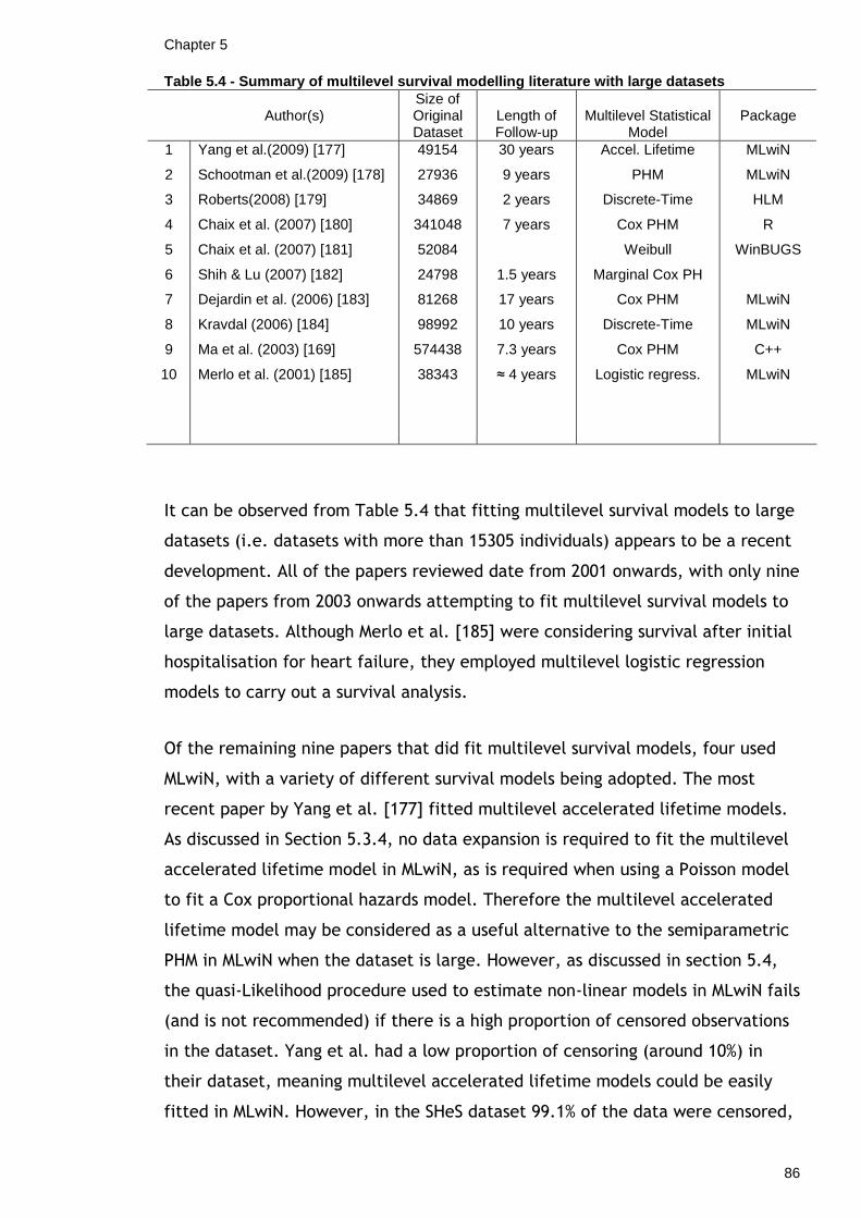
Chapter 5
86
Table 5.4 - Summary of multilevel survival modellin g literature with large datasets
Author(s) Size of Original Dataset
Length of Follow-up
Multilevel Statistical
Model
Package
1
2
3
4
5
6
7
8
9
10
Yang et al.(2009) [177]
Schootman et al.(2009) [178]
Roberts(2008) [179]
Chaix et al. (2007) [180]
Chaix et al. (2007) [181]
Shih & Lu (2007) [182]
Dejardin et al. (2006) [183]
Kravdal (2006) [184]
Ma et al. (2003) [169]
Merlo et al. (2001) [185]
49154
27936
34869
341048
52084
24798
81268
98992
574438
38343
30 years
9 years
2 years
7 years
1.5 years
17 years
10 years
7.3 years
≈ 4 years
Accel. Lifetime
PHM
Discrete-Time
Cox PHM
Weibull
Marginal Cox PH
Cox PHM
Discrete-Time
Cox PHM
Logistic regress.
MLwiN
MLwiN
HLM
R
WinBUGS
MLwiN
MLwiN
C++
MLwiN
It can be observed from Table 5.4 that fitting multilevel survival models to large
datasets (i.e. datasets with more than 15305 individuals) appears to be a recent
development. All of the papers reviewed date from 2001 onwards, with only nine
of the papers from 2003 onwards attempting to fit multilevel survival models to
large datasets. Although Merlo et al. [185] were considering survival after initial
hospitalisation for heart failure, they employed multilevel logistic regression
models to carry out a survival analysis.
Of the remaining nine papers that did fit multilevel survival models, four used
MLwiN, with a variety of different survival models being adopted. The most
recent paper by Yang et al. [177] fitted multilevel accelerated lifetime models.
As discussed in Section 5.3.4, no data expansion is required to fit the multilevel
accelerated lifetime model in MLwiN, as is required when using a Poisson model
to fit a Cox proportional hazards model. Therefore the multilevel accelerated
lifetime model may be considered as a useful alternative to the semiparametric
PHM in MLwiN when the dataset is large. However, as discussed in section 5.4,
the quasi-Likelihood procedure used to estimate non-linear models in MLwiN fails
(and is not recommended) if there is a high proportion of censored observations
in the dataset. Yang et al. had a low proportion of censoring (around 10%) in
their dataset, meaning multilevel accelerated lifetime models could be easily
fitted in MLwiN. However, in the SHeS dataset 99.1% of the data were censored,

Chapter 5
87
and hence the use of multilevel accelerated lifetime models in MLwiN for this
dataset would not be recommended.
Of the other three papers using MLwiN, other methods for fitting multilevel
survival models included the use of discrete-time models and the proportional
hazards model. Kravdal [184] used multilevel discrete-time hazard models to
analyse a Norwegian dataset consisting of 98992 individuals. The follow-up time
of 10 years was split into 6-month intervals, which the author deemed
reasonable having compared results to when time was grouped into intervals of 3
months. A wider discrete-time interval led to fewer risk sets. Dejardin et al.
[183] fitted a multilevel semiparametric proportional hazards model, which, in
MLwiN, is fitted via a Poisson model, to analyse a French dataset consisting of
81268 individuals. Although time was considered to be continuous, the unit of
time in this study (months), was larger than that considered in the SHeS dataset
(days). A larger unit of time may lead to a greater number of tied failure times,
and hence a smaller number of risk sets, thus resulting in a smaller dataset
following expansion. Dejardin et al. also stratified analysis, breaking up the
dataset into 12 separate cohorts which were analysed separately, with the
largest cohort consisting of 28010 individuals before data expansion. A criticism
of this paper is the estimation procedure adopted. First-order MQL was used to
estimate the multilevel Poisson model; however, as discussed in Section 5.3.5.3,
the MQL procedure may underestimate values of both the fixed and random
effects. Greater accuracy is to be expected when the second-order
approximation is used rather than the first-order, as adopted in this paper.
Finally, Schootman et al. [178] used MLwiN to fit multilevel survival models to a
dataset consisting of 27936 individuals; however, their analysis was stratified,
hence breaking up the dataset into five cohorts which were analysed separately.
The largest cohort then consisted of 7867 individuals. Models were estimated
using PQL estimation.
Five of the ten papers reviewed here used packages other than MLwiN to fit
multilevel survival models. Roberts [179] used the HLM6 program to fit
multilevel discrete-time survival models to three separate cohorts, the largest
containing 34869 individuals before data expansion. The size of this increased to
130961 following data expansion to obtain the person-period dataset. The
follow-up time of 2 years was grouped into 8 intervals of unequal numbers of

Chapter 5
88
days. In 2007, Chaix et al. [180, 181] wrote two separate papers using multilevel
survival models to model large Swedish datasets. The first [180] concerned a
dataset consisting of 341048 individuals, with a follow-up time of 7 years. The
full dataset was split into two cohorts depending on the age of the individuals,
thus leading to two cohorts comprising 192840 and 148208 individuals. The R
software was used to fit multilevel Cox proportional hazards models which were
estimated using a penalised likelihood method. The use of R for fitting multilevel
survival models was reviewed by Kelly [167], who concluded that R was useful if
only a single random effect was to be fitted. If more than one random effect was
desired, R would not be suitable. In the paper by Chaix et al., individuals were
nested within local areas; therefore, only one random effect was required,
meaning the R software could be used. A possible disadvantage of R is that the
random effect is limited to follow only a Gamma, Normal or t distribution.
However, this is not as restrictive as MLwiN, where the random effect may only
follow a (multivariate) Normal distribution. An advantage of the R software is
that it is free to download from http://www.r-project.org. In their second paper of
2007 [181], Chaix et al. fitted a multilevel Weibull survival model to a dataset of
52084 individuals. Models were estimated in WinBUGS using Markov chain Monte
Carlo (MCMC). WinBUGS was also reviewed in the paper by Kelly [167], who
discussed how any number of random effects could be fitted, with a number of
distributions being available for the random effects. WinBUGS is discussed
further in Section 7.4. Ma et al. [169] fitted a Cox PHM to a dataset of 574438
individuals via a Poisson model using a program written in C++. Parameter
estimates were obtained based on the orthodox best linear unbiased predictor
approach. Finally, Shih & Lu [182] considered a dataset containing 24798 Nepali
children. They fitted a two-level frailty model using a three-stage estimation
approach. It is not clear which software was used to estimate the model.
5.6 Chapter Summary
This chapter has shown how commonly used single-level survival models, such as
the proportional hazards model and the accelerated lifetime model, may be
extended to include random effects to account for hierarchical clustering. The

Chapter 5
89
use of several statistical packages for fitting multilevel survival models was
considered in Section 5.3.2, with MLwiN being acknowledged as the most
suitable package for fitting such models to a hierarchical structure. MLwiN is
able to fit both the proportional hazards model and the accelerated lifetime
model with the use of macros. As this thesis is concerned with fitting multilevel
survival models to large datasets, it was of interest to see how MLwiN would
perform when fitting multilevel survival models to such datasets. Section 5.4
displayed results obtained from fitting a multilevel proportional hazards model
to data from the 1995 and 1998 Scottish Health Surveys (SHeS) in MLwiN.
Interest was in measuring the association between GHQ-12 score and time until
first psychiatric hospital admission as measured from survey interview, following
adjustment for a range of demographic, socioeconomic and lifestyle risk factors.
The event of interest was rare meaning that there was a high percentage of
censored observations in the dataset (99.1%). In the presence of many censored
observations, Section 5.4.1 discussed how the quasi-likelihood under IGLS
estimation procedure tends to break down when fitting the multilevel
accelerated lifetime model. As a result, this model was not appropriate for the
SHeS data, and thus only the proportional hazards model was considered.
A multilevel continuous-time proportional hazards model was fitted to the SHeS
data in MLwiN via a Poisson model with log link function. Detailed information of
how the Poisson model was fitted in MLwiN was given in Section 5.3.3.1. In
particular, this included a discussion about how each duration had to be
expanded so that every individual had a series of records for each time point
until either the event of interest or censoring occurred (known as the person-
period dataset). This inevitably leads to an expansion in the size of the original
dataset and, in the case of the SHeS dataset which consisted originally of 15305
individuals, creating the person-period dataset led to an expanded dataset
consisting of approximately 1.9 million observations within individuals. MLwiN
coped with fitting the multilevel Poisson model to these data; however,
parameter estimates could only be obtained using the 1st-order PQL procedure
instead of the preferred 2nd-order PQL procedure.
The SHeS dataset was viewed as a moderately sized dataset, and therefore did
not prove to be too problematic. However, it can be envisaged that the data
expansion resulting from creating the person-period dataset could be vast if the

Chapter 5
90
size of the original dataset was already large (i.e. consisting of more individuals
than the SHeS dataset), and therefore perhaps leading to problems with
estimation. As health survey datasets are typically large, it is of interest to
investigate more efficient ways to fit multilevel survival models to large
datasets, and to ensure that these models are accessible to those working in
public health. Using the SHeS dataset as a training dataset for developing and
testing various methods, succeeding chapters will seek to establish the most
efficient ways of fitting multilevel survival models to large datasets. Successful
models will then be applied to a much larger dataset to confirm their
effectiveness.

91
6 Discussion: Findings from the Scottish Health
Survey
6.1 Introduction
The Scottish Health Survey (SHeS) dataset was linked with all psychiatric hospital
admission and death records between 1981 and 2004 for the purpose of
investigating the growing problem of mental disorder in Scotland. A review of
the literature (Chapter 3) revealed that there was a lack of information
available on risk factors for mental disorder in Scotland, and most of the
literature reviewed came from studies conducted elsewhere.
In Scotland, most of the information on mental health comes from acute and
psychiatric hospital discharge records. It therefore seemed appropriate to use
psychiatric admission as a measure of poor mental health in Scotland. Using the
linked SHeS dataset, it was possible to investigate risk factors for poor mental
health in Scotland, where a psychiatric admission would be an indicator of poor
mental health. The SHeS dataset contained information on a wide range of
demographic, socioeconomic and lifestyle risk factors and the specific objective,
using the SHeS data, was to investigate the association between the GHQ-12 (the
questionnaire used to assess the psychosocial health of respondents in the SHeS)
and psychiatric admission, while controlling for the numerous risk factors
available in the SHeS.
Since the Scottish Health Survey dataset was hierarchical in nature, with
respondents nested within postcode sectors, multilevel modelling techniques
were employed to overcome the problems discussed in Section 1.2.
6.2 Summary of Findings
The outcome was time until psychiatric admission as measured in days from
Scottish Health Survey interview. An unpublished Master of Public Health
dissertation by Stewart [30] revealed that the likelihood of psychiatric admission

Chapter 6
92
differed depending on whether the admission was a first admission or a
readmission. Based on this finding, it was appropriate to stratify analyses
according to whether or not respondents had any known history of psychiatric
admission. No known history of psychiatric admission prior to survey interview
implied that any psychiatric admission following survey interview was taken as a
first ever admission. Similarly, if a respondent had a known history of psychiatric
admission(s) prior to survey interview, then any admission following survey
interview was taken as a readmission. For reasons given in Section 4.1.1,
analyses focused only on risk factors for first psychiatric admission.
The first objective, as stated in Section 3.5, was to investigate the association
between the GHQ-12 and first psychiatric hospital admission in Scotland. Table
4.5 in Section 4.1.2 suggested that, subjectively, there appeared to be an
association between psychiatric admission and GHQ-12 score, with the indication
of a possible increasing trend. This trend was investigated formally in Chapters 4
and 5 by fitting various multilevel logistic regression (Table 4.6) and multilevel
survival models (Table 5.3). All results given in the tables listed indicated that
there was a highly significant increasing trend in the hazard (odds for the logistic
regression model in Table 4.6) of first psychiatric admission as GHQ-12 score
increased. The between-postcode-sectors variation was always small (although it
was large in comparison to the probability of psychiatric admission in the
average area). This finding was consistent with the reviewed literature, where it
was found by most that any variation between higher-levels, such as postcode
sectors, was indeed very small (Section 3.4).
The second objective, as stated in Section 3.5, was to investigate whether any
association between psychiatric admission and the GHQ-12 remained following
adjustment for a range of individual- and area-level demographic,
socioeconomic and lifestyle risk factors. There were a number of issues to
consider before fitting the models. In public health and epidemiology, it is
standard practice to control for sex and age when investigating the association
between a set of risk factors and an outcome. In view of this, it was decided to
include sex and age in every adjusted model, even if they were not significantly
associated with the outcome in addition to the other predictors. The second
issue concerned the over-controlling of variables in the models. Section 3.2.1.2
discussed how it had been shown that the GHQ correlated well with other self-

Chapter 6
93
administered questionnaires. As information on respondents’ self-assessed
general health was available in the SHeS, there was the possibility of over-
controlling if both GHQ-12 score and respondent’s rating of their self-assessed
general health were included in the model. In order to avoid this, models
adjusting for other various risk factors were fitted both including and excluding
self-assessed general health rating.
Fitting the various multilevel models (Tables 4.6 and 5.3) revealed that, when
self-assessed general health was excluded, the increasing trend in the hazard
(odds for the logistic regression model) of first psychiatric admission remained
highly significant following adjustment for a range of, in the first instance,
individual-level risk factors. Significant risk factors associated with an increased
hazard of first admission (in addition to GHQ-12 score of one or more) included
not being married (i.e. single, separated, divorced or widowed), being in receipt
of benefits, and being a current smoker. Sex and age were not significantly
associated with the outcome in addition to the other significant variables;
however, they were included in the model for reasons discussed above.
Employment status was bordering on significance; therefore, it was kept in the
model. When the two area-level risk factors were added to the model including
all significant individual-level risk factors, neither was associated with the
outcome. The area-level risk factors comprised a measure of area deprivation
(Carstairs score) and a measure of urbanicity. The multilevel logistic regression
model indicated that this model explained 22% of the total unexplained variation
between postcode sectors.
When the same models were refitted with self-assessed general health allowed
as a potential risk factor, results were similar to those when self-assessed
general health was excluded. The effect of GHQ-12 score on the hazard (odds for
logistic regression model) was attenuated when self-assessed general health was
included; however, the increasing trend remained significant. Significant
individual-level risk factors also remained the same; however, this time, being
unemployed, and having a self-assessed general health rating other than ‘very
good’ (i.e. ‘good’, ‘fair’, ‘bad’ or ‘very bad’), were also among the individual-
level risk factors associated with an increased hazard (odds) of first psychiatric
admission. Again, neither of the area-level risk factors was significantly

Chapter 6
94
associated with the outcome when added to the model including all significant
individual-level risk factors.
The results found here are not unexpected, and are fairly consistent with the
literature. Section 3.3.1 highlighted discrepancies in the literature on the
effects of demographic risk factors, such as sex and age, on mental disorder and
psychiatric admission. Some authors reported significant associations between
sex and mental disorder and age and mental disorder; other studies reported no
significant associations. A number of studies conducted outside the UK [65, 72,
73] reported similar results to those found here, with no difference in admission
to psychiatric facilities found between the sexes. A study conducted in the UK by
Jarman et al. [66], which may be more comparable to the results found in this
study of Scotland, also reported similar national psychiatric admission rates for
men and women. However, a study conducted in England by Thompson et al.
[75] did find differences in admission rates between the sexes, with higher rates
being reported for males. The study by Thompson et al. was quite different from
this study in that interest was in investigating patterns of psychiatric admission
by age, gender, diagnosis and regional health authority, rather than
investigating risk factors for psychiatric admission. Therefore they did not adjust
for any socioeconomic or lifestyle predictors known to affect psychiatric
admission. Thus, although the finding by Thompson et al. is not consistent with
that found here in Scotland, the studies are not directly comparable. It may be
somewhat surprising that sex was not found to be significant in this study as it
has been suggested in the literature [68] that females suffer more from disorders
that do not require hospitalisation (i.e. neurotic disorders). As a result, it may
have been expected to find that males had a greater likelihood of psychiatric
admission.
Marital status was found to be significantly associated with psychiatric admission
in addition to a range of other risk factors. Indeed, it was shown that those in
the ‘not married’ category, which included single, separated, divorced and
widowed persons, had a higher likelihood of psychiatric admission than their
married counterparts. This finding is consistent with the literature, with all of
the reviewed literature reporting the lowest risk of mental disorder for married
persons. It was also noted in the literature that married persons are more likely
than single persons to be treated in the community [79]. It is therefore possible

Chapter 6
95
that the significance of this risk factor only represents differing patterns of
treatment (i.e. treatment in the community as opposed to inpatient admission)
and not a greater likelihood of mental disorder.
In terms of socioeconomic risk factors for psychiatric admission, it is difficult to
make direct comparisons between findings in this study and findings from other
studies, as the range of socioeconomic factors varied between the studies
reviewed. Apart from income, this study included all of the conventional
measures of socioeconomic position (social class, education, material
circumstances, employment status), whereas most of the reviewed literature
included only one or two measures of socioeconomic status. An exception to this
was the study by Lahelma et al. [58], which included a wide range of measures
of socioeconomic position at childhood and adulthood. Indeed, Lahelma et al.
commented that ‘socioeconomic measures are not directly interchangeable and
any single indicator is unlikely to provide a sufficient description of past and
present socioeconomic circumstances’. Socioeconomic risk factors found to be
associated with psychiatric admission in this study were receipt of benefits and
employment status. Socioeconomic risk factors that were not significant in the
model included social class of the chief income earner, years spent in education,
top academic qualification and material circumstances. The latter corresponded
to car and home ownership. It was not altogether surprising that a lot of these
variables were not significant in the model in addition to each other, as high
correlation between the variables is to be expected. For example, it would be
expected that persons who spent the fewest years in education would have the
lowest qualifications. This, in turn, may lead to poorer job opportunities, making
car and home ownership difficult; or, indeed, the lowest qualified persons may
be unemployed and thus receiving benefits. It is perhaps, therefore, somewhat
surprising that both employment status and receipt of benefits were both
significant in the model. The results indicated that unemployed persons and
persons in receipt of benefits had an increased likelihood of psychiatric
admission. It was not surprising that employment status was found to be
significantly associated with the outcome, as there is a long history of interest in
the association of this variable with mental disorder acknowledged in the
literature [30, 87, 92, 96, 101]. If unemployment and receipt of benefits are
taken to be representative of low socioeconomic position, then these findings

Chapter 6
96
were in line with those of Kammerling & O’Connor [96] and Dekker et al. [97],
who recognised a long-standing association between low socioeconomic position
and admission to psychiatric hospital.
A number of ‘lifestyle’ variables such as average weekly alcohol consumption,
smoking status and weekly participation in sports were also included as potential
risk factors. Smoking status was the only lifestyle variable found to be
significantly associated with first psychiatric admission in this study (Tables 4.6,
5.3). Again, it may not be surprising that not all of the lifestyle variables were
significant in the model as there could be some correlation between them. For
example, smoking status and alcohol consumption are usually correlated, with
smokers tending to drink more and heavy drinkers tending to smoke more [186-
188]. This unhealthy lifestyle may also imply that those persons would be less
likely to participate in physical exercise. Findings from this study indicated that
current smokers had an increased hazard (odds) of first psychiatric admission. No
significant differences were found between non-smokers and ex-smokers.
Findings from this study were consistent with those of Rasul et al. [108], Araya
et al. [107] and Cuijpers et al. [105], who also reported a greater likelihood of
mental disorder in current smokers. In addition, Araya et al. [107] reported no
difference between non- and ex-smokers. However, these studies all referred to
common mental disorders and therefore findings may not be directly comparable
to those in this study if psychiatric admission is viewed more as a measure of
major mental disorder. However, the study by Cuijpers et al. that found an
association between common mental disorder and smoking found no association
between smoking and incidence of major depression. On the other hand, Breslau
et al. [106] did report an association between major mental disorder and
smoking; however, they found an increased risk in both current and ex-smokers.
A number of studies also suggested that the risk of mental disorder in current
smokers increased even more as the number of cigarettes smoked increased
[107, 108]; however, these data were not requested when applying to the
Information and Services Division Scotland (ISD Scotland) for the Scottish Health
Survey data to be used in this study (refer to Section 2.2 and Table 2.1).
As well as smoking status being an indicator of a poor or healthy lifestyle, it
should be recognised that it may also be a measure of poor socioeconomic
position. Many studies have reported that inequalities in smoking habits exist,

Chapter 6
97
with low socioeconomic position being associated with a higher prevalence of
smoking [189-192]. Smoking status has also been shown to be associated with a
number of other measures of socioeconomic position. In particular, level of
education [189-192] and occupational class [189, 190, 192] have been shown to
be inversely associated with smoking status. These associations may also explain
why not many of the socioeconomic risk factors in this study were significant in
the model in addition to each other.
The final objective was to determine the ‘best’ threshold score for use of the
GHQ-12 in Scotland. Section 3.2.1.1 noted that Goldberg suggested that a score
of 1 or 2 was the optimal threshold score, as found by his original validity study
in the UK in 1972 [45, 50]. However, many studies since this time suggested
different threshold scores. As it is generally accepted that threshold scores vary
between different settings, cultures and populations (reference list given in
Section 3.2.1.1), it is not at all surprising that findings in the literature were
inconsistent. In the published reports from the 1995 and 1998 Scottish Health
Surveys [23, 25], a score of four or more was used to identify respondents with a
high GHQ-12 score, and thus at risk of potential psychiatric disorder. However,
using the 1995 and 1998 linked SHeS data, this study found that the hazard
(odds) of first psychiatric admission was significantly increased in those scoring
one or more in the GHQ-12 (Tables 4.6 and 5.3). This remained the case even
after adjustment for a range of demographic, socioeconomic and lifestyle risk
factors. Therefore, findings from this study suggest that a score of one or more
is the ‘best’ threshold score for indicating high GHQ-12 score in the Scottish
population. This fits in with Goldberg’s original validity study in the UK, as
discussed in Section 3.2.1.1. However, if GHQ-12 is being used to predict the
likelihood of psychiatric admission, then a threshold score of one or more would
put a lot of people, perhaps falsely, at risk of psychiatric admission. Other
studies have also reported that the GHQ-12 can produce a high rate of false
positive results (Section 3.2.1.2), and therefore should be combined with other
screening instruments. The combined use of the GHQ-12 and other screening
instruments would also be recommended based on results from this study.

Chapter 6
98
6.3 Limitations
6.3.1 Limitations of Data
Section 2.2 acknowledged that there could be weaknesses associated with using
the linked SHeS-SMR04 dataset that could have implications for analyses. These
weaknesses will now be considered. The first weakness is that of non-response
to the survey interview. This is a potential source of bias since characteristics of
responders may differ to those of non-responders. For the 1995 and 1998 SHeS,
response rates to the individual survey interviews were 81% and 76%
respectively. Generally it was found that women were more likely to respond
than men, younger ages were the most likely to refuse and response rates
decreased as level of urbanicity increased [23]. Weights were used in order to
account for the differing rates of response between the sexes, age groups and
regions. As with any survey, there were some respondents in the SHeS who
refused to answer specific questions or have a biological measurement taken,
thus leading to missing data. Furthermore, a small percentage of respondents (7-
9%) refused permission to linkage. It may be that the decision to refuse, either
to answering a question or to data linkage, is socially or geographically
patterned which could bias results obtained from analysing these data. Using the
1998 SHeS dataset, Lawder et al. [27] investigated this notion by excluding all
cases with missing values in any variables and reported that respondents for
which complete survey data were available tended to be healthier (in terms of
vegetable consumption, blood pressure, BMI measurements, general health and
longstanding illness), less deprived, less likely to be on benefits, more likely to
own their own home, better educated and of a higher social class. These findings
suggest that refusal is socially patterned and that complete case analysis would
lead to biased results since the sample would not be representative of the
population of Scotland. It may be possible to overcome this by employing
appropriate techniques for handling missing data, such as multiple imputation.
This may lead to a more representative sample of the population of Scotland.
Another source of potential bias with using the linked SHeS-SMR04 dataset is
emigration. As respondents to the SHeS are followed-up long after their survey
interview, it may be possible that their SMR records are incomplete at the date
Chapter 6
99
of linkage to the SHeS if they have emigrated subsequent to survey interview.
Although emigration levels in Scotland generally tend to be low [22], there is a
procedure in order to determine potential emigrants during the linkage process.
This procedure involves linking the SHeS to the Community Health Index (CHI) in
order to determine whether respondents are registered with a Scottish General
Practice at the end of the SMR follow-up period [24]. Lawder et al. [27] reported
that of the 15668 respondents to the 1995 and 1998 surveys who agreed to
linkage, 15446 (98.6%) still linked to CHI in March 2005 (which is beyond the
follow-up period for the Scottish dataset in this thesis). Although it is important
to take emigration into consideration since characteristics of emigrants may be
different to other individuals in the survey, Lawder et al. showed that including
or excluding emigrants from modelling would only have a minimal impact on the
results.
It is generally acknowledged that using cross-sectional data may be a limitation
since it implies that no inferences about causal pathways can be made from the
results [135, 137, 138, 140, 142]. Although the SHeS is cross-sectional, events
are recorded following survey interview and therefore risk factors precede
psychiatric admissions. However, as individuals who are mentally ill could be
undiagnosed at the time of survey interview it is unclear as to whether risk
factors precede psychiatric disorder. In particular, many studies have queried
the direction of the relationships between marital status and mental disorder,
and measures of socioeconomic circumstances and mental disorder. These
queries will now be considered.
Marital status has been shown by many, as well as by this study, to be
significantly associated with mental disorder, leading to the conclusion that
persons in any category of marital status, other than married, were at higher
risk of disorder (see Section 3.3.1 for references). However, as analyses were
performed on cross-sectional data in most of these studies, authors were unable
to comment on the direction of the association. Many authors have considered
two hypotheses in an attempt to explain the association between mental
disorders and marital status. They are most commonly known as the ‘selection
hypothesis’ and the ‘protection hypothesis’. The selection hypothesis argues
that constitutional traits of persons who develop mental disorders, even before
its outbreak, may inhibit marriage [76, 81, 83, 193]. The protection hypothesis,

Chapter 6
100
on the other hand, argues that marriage offers a degree of protection against
conflict, even for those with constitutional traits, which in non-married persons
may lead to an outbreak of mental disorder.
There are similar hypotheses attempting to explain the association between
socioeconomic deprivation and mental disorder. These hypotheses are known as
the social segregation hypothesis or ‘drift’ effect and the social causation
hypothesis, or ‘breeder’ effect. The ‘drift’ effect argues that people already
with a mental disorder are more inclined to move towards poorer areas, whereas
the ‘breeder’ effect argues that factors, such as socioeconomic deprivation,
encourage and exacerbate mental disorders [73, 83, 89, 194].
Similarly, there have also been suggestions of a ‘two-way’ relationship between
smoking status and mental disorder; in particular, depression. Depression has
been shown to be associated with initiation of smoking; conversely, however, it
has also been shown that nicotine may increase the risk of mental disorder
[195].
Another limitation of the linked SHeS dataset corresponds to the definition of
‘first psychiatric admission’. In this study, any admission recorded following
survey interview was assumed to be a first admission if the respondent had no
record of psychiatric admission prior to survey interview. However, psychiatric
admission records were only available from 1981 onwards, and as a result
information on any psychiatric admission(s) occurring prior to 1981 was
unavailable. Consequently, when respondents were defined as having had no
admission prior to survey interview, this definition only truly referred to having
had no psychiatric admission since 1981. This issue is further affected by
immigrants moving to Scotland from other countries. As information on any prior
admissions outside of Scotland is unavailable, immigrants would be coded as
having no prior psychiatric admission even though they may have been admitted
to psychiatric facilities in their home countries. Similarly, individuals who
migrate to other countries before the end of follow-up and subsequently
experience a psychiatric admission in another country will have no outcome
recorded (and will be censored when modelling the data using survival analysis).

Chapter 6
101
6.3.2 Limitations of Variables and Analyses
A number of variables, suggested by the literature as being potentially important
risk factors for mental disorder, were not available in this study. In particular,
these included ethnicity and diagnostic group. Although ethnic group was
recorded in the SHeS, the number of respondents classed in minority groups (i.e.
non-white) was very small (<1%). It was therefore not possible to investigate the
effect of ethnicity on psychiatric admission. As a result, this variable was
discarded. Discarding this variable may have led to a loss of potentially
important information since it has been shown by some that ethnic group may be
associated with mental disorder [89, 96].
Diagnostic group has been shown by some to be associated with psychiatric
admission; however, information on diagnostic group was not requested when
applying for the SHeS dataset. Thompson et al. [75] found that depression and
anxiety was the primary diagnosis given at admission, followed by schizophrenia
and related psychoses. In addition, diagnosis has been shown to vary by gender.
Both Timms [73] and Saarento et al. [74] discussed that, generally,
dependencies and schizophrenia occurred more frequently in males, whereas
neuroses and affective psychoses were more common in females. It may
therefore have been of interest to investigate for a possible interaction between
sex and diagnostic group, had information on diagnostic group been available.
As well as the suggestion of an interaction between diagnostic group and sex,
there were a number of other potentially important interactions suggested by
the literature. In particular, the most consistent findings included the following
interactions. The first was between age and sex, where it was found by
Thompson et al. [75] that the ages at which admission rates peaked differed for
males and females; however, this was not supported by Kirshner & Johnston
[72], who found no interacting effect of sex and age on admission. The second
was between sex and marital status, where it has been suggested that the effect
of marital status on admission differs by sex. It has been shown that males have
higher rates of admission than females in every category of marital status except
‘married’, where it has been shown that males have lower rates of admission
[82, 196]; however, Kirshner & Johnston [72] did not support this finding. There

Chapter 6
102
was also the suggestion of a three-way interaction between sex, age and marital
status [79, 80]. Due to time constraints, this study did not test for interactions
between any combinations of variables since the purpose of the thesis was
focussed more on the development of methods for fitting multilevel event
history models, rather than providing a comprehensive investigation of
psychiatric admissions.
Another interesting risk factor for admission which was not included in analyses,
but possibly should have been, was survey year i.e. the year in which
respondents took part in the SHeS, which would have been either 1995 or 1998.
Although fitting survival models accounted for the differing lengths of follow-up
time between the two surveys, inclusion of this variable may have demonstrated
the changing patterns in psychiatric admission. If results had shown that
respondents who took part in the 1998 survey had a smaller likelihood of
admission than those in the 1995 survey, then this may have been a reflection of
the shift from inpatient admission to treatment in the community.
In this study, the primary objective was to investigate the association between
the GHQ-12 and first psychiatric hospital admission. However, there is a possible
limitation with using this as the outcome measure. This concerns the changing
patterns in psychiatric admissions with a shift from inpatient admissions to care
in the community. In a study investigating geographical variations in the use of
psychiatric inpatient services in New York, and how they have changed from
1990 to 2000, Almog et al. [197] noted that differences in rates of admission
between certain population groups may have resulted from an inadequacy in
access to community care. Thus, if people in more advantaged areas have better
access to psychiatric care in the community and make use of this service instead
of inpatient psychiatric care, then it may appear that admissions are higher in
disadvantaged areas. Indeed, this study found that those of low socioeconomic
position had a greater likelihood of psychiatric admission.

Chapter 6
103
6.4 Recommendations for Future Work
A discussion of the limitations of this study in Section 6.3 suggested a number of
recommendations for future work. The first recommendation concerns
interactions between variables. Section 6.3.2 discussed a number of interactions
between individual-level risk factors which were consistently found to be
associated with mental disorder in the literature, but which were not
investigated in this study. Therefore, this study could be developed further by
including interactions between individual-level risk factors, random slopes to
investigate how the association between each risk factor and first psychiatric
admission varies across areas and cross-level interactions, i.e. interactions
between individual- and area-level risk factors in the analyses.
Another recommendation concerns the outcome measure used. It should be
decided before the study whether interest lies in investigating common mental
disorder or serious mental disorder. Since the outcome measure here was
psychiatric admission, this suggests that interest was in investigating more
serious mental disorder, since, as has been discussed throughout the thesis,
there is now the tendency to treat more common mental disorders in the
community. This means that all findings from this study may only truly apply to
serious mental disorders. However, if interest were in investigating risk factors
for all mental disorders together, then GHQ-12 score might be a more
appropriate outcome variable, since this study has shown that GHQ-12 score is
associated with serious mental disorder, as well as common mental disorders, as
was suggested by the literature.
Finally, if any further work was to be done with the same subset of Scottish
Health Survey data as used in this study, it would perhaps be worthwhile
reapplying to ISD Scotland for information on other potential risk factors of
psychiatric admission. In particular, it may have been useful to have information
on psychiatric diagnosis (and perhaps on the number of cigarettes smoked per
day as discussed in Section 6.2).

Chapter 6
104
6.5 Implications of the Findings
A literature review of risk factors for mental disorder and psychiatric hospital
admission (Section 3.3) revealed that there was a paucity of information for the
Scottish population and indeed almost all of the reviewed literature came from
studies conducted outside Scotland. Although findings from studies conducted
outside Scotland provide valuable information on risk factors for psychiatric
admission, the generalisability of these findings to other populations, in this
instance, the Scottish population, is always questionable since it is unlikely that
risk factors affecting psychiatric admissions in one population will be identical to
those in another. This may be a consequence of differences in management and
diagnosis between populations. Therefore, one of the most important
contributions that the findings from this study will make will be in providing a
basis for which future studies of risk factors for psychiatric admissions in the
Scottish population can refer to and build on. A proviso would be increased
availability of information in Scotland. Increasing and expanding the amount of
information on risk factors for psychiatric admission may have implications for
both future research in studies conducted in Scotland and elsewhere, and future
mental health policies and programmes in Scotland. For example, this study
showed that low socioeconomic position was associated with first psychiatric
admission. As a result, public health policies for mental health should, in
particular, be targeting the most deprived individuals in Scotland. This may lead
to a reduction in mental health inequalities between the poorer and more
affluent socioeconomic groups.
Improving mental health may also lead to an improvement in other poor health
behaviour, such as smoking. In this study smoking was shown to be associated
with mental disorder, as measured by psychiatric admission. Smoking has been
shown to be used as a ‘coping mechanism’ in order to manage depression and
stress [191]; therefore, this would imply that an improvement in mental health
may lead to a reduction in the need for coping mechanisms, such as smoking.
The primary finding of this study was that GHQ-12 score was associated with first
psychiatric admission. With common mental disorders now tending to be treated
in the community rather than in a hospital, psychiatric hospital admission is

Chapter 6
105
perhaps more representative of more serious mental disorder. However, findings
from the literature recommended that the GHQ only be used for detection of
minor psychiatric disorder [49, 51, 58]; therefore, findings from this study are
particularly interesting as they suggest that the GHQ is also associated with
more serious mental disorder, as represented by a psychiatric admission. Hence,
another implication of the findings is the use of the GHQ for detection of more
serious mental disorders.
6.6 Conclusions
This study has shown that the GHQ-12 is significantly associated with first
psychiatric hospital admission in Scotland, even after adjustment for a range of
demographic, socioeconomic and lifestyle risk factors. Multilevel models allowed
the variation in the hazard of first psychiatric admission to be partitioned into
that attributable to differences between individuals and that attributable to
differences between postcode sectors. The between-postcode sector variation
was always found to be small, a finding that was consistent with the literature.
This study suggested that a score of 1 or 2 on the GHQ-12 was the optimal
threshold score for defining psychiatric caseness in the Scottish population. This
was consistent with Goldberg’s original validity study carried out in the UK in
1972; however, it was perhaps not consistent with all of the other reviewed
literature. This is not worrying given that variation in optimal threshold scores
between different populations and cultures is to be expected, as was discussed
in Section 3.2.1.1.
In conclusion, this study has provided a basis for which future studies of mental
disorder in the Scottish population can refer to and build on, as well as
highlighting groups most at risk of poor mental health, such as those of a low
socioeconomic position. These groups need to be targeted in order to improve
mental health in Scotland and reduce health inequalities between poorer and
more affluent areas. The GHQ-12 may be used as a screening instrument to
identify those at risk of potential psychiatric caseness for both common and
more serious mental disorders.

106
7 Alternative Methods for Fitting Multilevel
Survival Models to Large Datasets
7.1 Introduction
Chapter 5 discussed ways in which multilevel survival models can be fitted in
MLwiN – a package specially designed for fitting multilevel models to hierarchical
datasets. To fit a proportional hazards model, one of the most commonly used
continuous-time survival models for modelling the effect of covariates on
survival time, MLwiN adopts a Poisson modelling approach. As discussed in
Section 5.3.3.2, a person-period dataset must be created in order to fit the
Poisson model. This involves replicating each individual’s record as many times
as the observed number of time intervals, either until the event of interest or
censoring occurs for that individual. Clearly, this leads to an expansion in the
size of the original dataset which can become problematic for reasons discussed
in Section 5.6. It is therefore of interest to investigate other methods which
could be used as an alternative to fitting continuous-time multilevel proportional
hazards models. Three possible alternatives will be considered in this chapter.
These three methods will then be fitted to the SHeS dataset in order to test
their effectiveness as alternatives to the continuous-time model. Results are
given in Chapter 8.
7.2 Defining Different Risk Sets
7.2.1 Introduction
The first method to be considered, as an alternative to fitting continuous-time
hazard models, involves defining different risk sets. When expanding the dataset
in order to fit continuous-time hazard models, each individual event time was
considered as a separate risk set. As a result, the size of the expanded dataset
could become very large if there were a lot of events. Instead of considering
each event as a separate risk set, one alternative is to consider all events

Chapter 7
107
within, for example, a month or a year or any other length of time interval. This
is achieved by dividing time into short intervals so that risk sets now correspond
to each predetermined interval. Using this method involves fitting discrete-time
models and it is expected that dividing time into short intervals and fitting
discrete-time models will lead to a reduction in the size of the expanded
dataset.
There are a number of other reasons why discrete-time models are favoured
over continuous-time models. Firstly, accommodating tied observations (i.e.
when two or more individuals experience the event of interest at the same time)
is more straightforward using a discrete-time approach. In the SHeS data, tied
observations were not a problem as there were so few events and the scale used
to record time was so small (i.e. event times were recorded in days) making it
unlikely that two or more individuals would have been admitted to psychiatric
facilities at the same number of days from survey interview. However, if there
are a lot of events in the dataset and the scale used to record time is longer,
months, for example, then there is the potential for tied observations to occur.
The use of continuous-time models in the presence of tied observations is
inappropriate as inconsistent estimators can result [198]. Incorporation of time-
varying covariates is also more straightforward using the discrete-time approach.
Finally, following some restructuring of the data so that the response variable is
binary (see Section 7.2.2), standard methods for fitting discrete response data,
such as logistic regression, may be used to fit discrete-time models.
As mentioned above, the logit link function can be used to model the
dependence of the hazard rate on time and explanatory variables; however,
other link functions, such as the complementary log-log function, may also be
used. If time is divided into meaningful discrete intervals, then the logit link is
used; however, if an event occurs at an exact time, but the measurement of
time is coarse (for example, if it is rounded to the nearest month), then this is
referred to as grouped-time, and the complementary log-log link function should
be used [199]. The complementary log-log link may also be preferred as the
coefficient vector is invariant to the length of time intervals [156, 200];
however, the logit link may be favoured because of its computational
convenience, and also because it is easy to interpret in terms of odds ratios
[201]. Generally, however, the choice of link function does not matter as both

Chapter 7
108
produce similar results, leading to the recommendation that the choice be based
on ease of interpretation [202, 203].
7.2.2 The Multilevel Discrete-Time Model
7.2.2.1 Fitting Multilevel Discrete-Time Survival M odels in MLwiN
Section 7.2.1 remarked that standard methods for fitting discrete response data
may be used to fit discrete-time models. This means that any statistical package
that can perform regression analysis of dichotomous response variables can be
used to fit discrete-time hazard models. However, as the hierarchical structure
of the Scottish Health Survey data must be incorporated into the model, a
multilevel discrete-time model must be used. As discussed in section 5.3.2,
MLwiN is a package specifically designed for fitting multilevel models; therefore,
it is reasonable to use it to fit the (multilevel) discrete-time models.
Assuming that time is divided into p intervals (not necessarily of equal length),
It = [at-1, at) with 0 = a0 < a1< . . . <ap < ∞, with discrete time T=t where t in 1,
. . . , p denotes an observed event in interval It. Then the discrete hazard
function for individual i in postcode sector j is
( ) ( )( ) ( ) ( ) j
q
ptpijpjtij utfxutfxthg +++= ∑
=10,,; βββ ,
where xij(t) is a vector of (possibly time-varying) covariates, β is a vector of
parameters to be estimated and represents the effect of the covariates on the
baseline hazard (on the scale generated by g(.)), uj is the random-effect for
postcode sector j, and is assumed to be Normally distributed with mean 0 and
variance σu2, and, finally, f(t) is a function of time used to model the baseline
hazard function. Possible forms for f(t) will be discussed in Section 7.2.2.3.

Chapter 7
109
Because of its computational convenience and ease of interpretation, the logit
link will be adopted as the link function for g(.) when fitting the multilevel
discrete-time models in MLwiN. Therefore, the model can be written as
( )( ) ( )( ) ( ) ( ) j
q
ptpijpij
ij
ij utfxthitth
th+++==
− ∑=1
0log1
log ββ ,
Equation 7.1
where the logit-hazard, logit(hij(t)), refers to the log-odds of event occurrence in
any time interval, given that the event has not already occurred prior to this
time. This model is known as a proportional odds model. The proportional odds
assumption will be discussed in Section 7.2.3. Petersen [157] noted that the
coefficients estimated from a logit model may not be entirely comparable with
those obtained from a continuous-time model; however, as discussed by
Petersen, Willet & Singer [204] and Hank [205], if the conditional probability
that an event occurs in time interval t (given that it has not occurred prior to
this time) is small (Hank suggests no larger than 0.1), then the coefficients
obtained from the discrete-time model will be similar to those obtained from
the continuous-time model, and therefore the logit model can be viewed as
providing a good approximation to the continuous-time proportional hazards
model [205, 206].
In order to fit a discrete-time model, the data must first be expanded so that
every individual’s record is replicated as many times as the observed number of
time intervals before experiencing the event of interest or being censored. As
seen with the continuous-time data in Table 5.2, the original dataset can
become very large after expansion; however, in the discrete-time case, time is
restructured into intervals where each time interval represents a risk set,
instead of treating each separate event time as a risk set as in the continuous-
time case. This means that the expanded dataset in the discrete-time case will
be smaller than in the continuous–time case since there will be fewer risk sets.

Chapter 7
110
During the data expansion process, a set of dummy variables, yij(t), are defined
for individual i in group j so that
Therefore, if an individual does not experience the event, they will have a
sequence of zeros for every risk set, including a zero in the final risk set
indicating they were ultimately censored. On the other hand, if an individual
does experience the event, they will have a sequence of zeros for each risk set
prior to experiencing the event, and then a value of one for the risk set during
which the event occurred. Once an individual experiences the event, data
collection terminates for this individual. Fitting a discrete-time hazard model is
thus equivalent to fitting a binary response model on the expanded dataset.
When the hazard is modelled using the logit link, the parameters represent the
additive effects on the log odds of event.
Section 7.2.1 remarked that time-varying covariates could be easily incorporated
into a discrete-time model. Time-varying covariates are covariates which change
over time, such as age. The values of these covariates may vary between
intervals, but should remain constant within each time interval. Time-varying
covariates can be included in the model as interactions between fixed-time
covariates and time [200]. A time-varying covariate implies that the proportional
odds assumption is no longer valid. This will be discussed further in Section
7.2.3.
Because discrete-time models are fitted using standard models for binary
response data, such as logistic regression, an approximate intraclass correlation
(i.e. the proportion of the total variance that is accounted for by the higher-
level units) may be calculated as follows:
( )22
2
σσσ+
=U
UICC .

Chapter 7
111
When the logit link is used, the standard variance σ2 = π2/3 [203]. Alternatively,
if the complementary log-log link is used, σ2 = π2/6 [203]. Further information on
the intraclass correlation can be found in Section 4.2.
7.2.2.2 Determining the Length of Time Intervals
Section 7.2.2.1 discussed how the original dataset must be restructured so that
each individual has a line of data corresponding to each risk set until failure or
censoring occurs in order to fit the logistic model. As with continuous-time
models (refer to Section 5.3.3.2 for information on data expansion in the
continuous-time case), this restructuring inevitably leads to an expansion in the
size of the original dataset. When time is grouped into discrete intervals so that
there are fewer risk sets (with the number of risk sets being equal to the number
of discrete-time intervals) than in the continuous-time case, the discrete-time
person-period dataset still has the potential to be very large in size if the width
of the intervals is short relative to the observation period [207, 208]. One way to
reduce the size of this dataset is to increase the length of the intervals. This will
lead to fewer intervals, hence fewer risk sets, and thus the size of the expanded
person-period dataset will be reduced. Diamond et al. [209] found that little
precision was lost by grouping durations into reasonably broad groups.
It should be noted also that each time interval need not be of equal length. If
the data are restructured into time intervals corresponding to when event times
occur, then each interval will vary in length. On the other hand, it may be
appropriate to divide time into predetermined intervals, such as months, or
calendar years, etc, depending on the nature of the study, thus leading to
intervals of equal length.
7.2.2.3 Modelling the Baseline Hazard Function
In Equation 7.1 in Section 7.2.2.1, f(t) was written to denote the baseline hazard
function. Several forms can be considered for f(t), as was also noted in Section

Chapter 7
112
5.3.3.3. To recap, some of the possible forms, as discussed in Section 5.3.3.3,
included fitting a polynomial function, blocking factors, or some parametric
form could be assumed, such as the Weibull or Exponential distribution. When
fitting the continuous-time models in Chapter 5, a polynomial function was used.
It would not have been practical to use blocking factors in this case because of
the large number of risk sets. Blocking factors are a set of dummy variables for
the risk sets, written as
α1Z1 + α2Z2 + . . . + αlZl ,
where the α’s are parameters to be estimated and, for g = 1, . . . , l,
As there are tg or tg-1 dummy variables, using them in the continuous-time case
would have meant that a large number of parameters would have to have been
estimated. However, in the discrete-time case, where time has been grouped
into a few intervals, it is recommended that the blocking factor approach be
used [163]. In the logistic discrete-time model the α parameters thus represent
the baseline hazard in each time interval as measured on a logistic scale.
7.2.3 Assumptions
As in the continuous-time case, fitting discrete-time models also requires a
proportionality assumption. When a logit link is used as the link function, the
proportionality assumption is termed the ‘proportional odds’ assumption. The
proportional odds assumption is comparable to the proportional hazards
assumption in a model for the log-hazard, and for it to be valid requires that the
effect of a covariate is the same at all time points [199]. The proportional odds
assumption is tested by including interaction terms between predictors and time
in the model. The presence of a significant interaction implies non-
proportionality, thus indicating that a covariate is time-varying.

Chapter 7
113
As noted above, testing the proportional odds assumption is straightforward for
single-level discrete-time models. However, as discussed in Reardon et al. [199]
testing the proportionality assumptions becomes more complex in the multilevel
case. Reardon et al. remarked that, as well as testing whether the effect of
individual-level covariates on the hazard function is constant at all time points,
testing whether the effect of higher-level covariates is constant at all time
points must also be considered. They also discussed how multilevel models
include an additional proportionality assumption, which they termed the
‘proportional error assumption’, the assumption that the higher-level error term
for group j is constant at all time points. Full details of these assumptions and
how they can be tested can be found in their paper.
7.2.4 Estimation
Maximum likelihood is the most widely used approach for estimating the
parameters in the multilevel discrete-time model [201]. As the multilevel
discrete-time model is non-linear, approximate estimation procedures are used.
The two procedures available in MLwiN are marginal quasi-likelihood (MQL) and
penalised quasi-likelihood (PQL). Refer to Section 5.3.5 for a full discussion of
these procedures.
7.3 Grouping According to Covariates
7.3.1 Introduction
The second method to be considered as an alternative to fitting continuous-time
proportional hazards models involves grouping individuals within postcode
sectors according to values of their covariates and fitting continuous-time
hazard models in MLwiN to the grouped dataset. This method entails grouping all
individuals in the same postcode sector with the same values for covariates
being fitted in a particular model and creating one line of data for these
individuals as opposed to having a line of data for each individual. The concept

Chapter 7
114
behind this method is that all individuals within the same postcode sector with
the same values for covariates included in a particular model are at risk at the
same time, and can therefore be represented by one line of data, so that the
size of the expanded dataset can be reduced.
When individuals are aggregated according to their characteristics there is a
slight change in the nesting structure. In the case of the SHeS dataset there are
still two levels, with postcode sectors remaining at the higher-level (level 2).
However, at level 1 there is now a pseudo-level of cells defined by each possible
combination of the chosen characteristics. For example, in the case of model B1
(Table 5.3) where GHQ-12 is the only covariate in the model, each level 1 ‘cell’
corresponds to one category of GHQ-12 score (score of 0, 1-2, 3-4 or 5-12).
However, suppose the covariate ‘sex’ (where the choice is either ‘male’ or
‘female’) is added to this model. This means that there is now a cell
corresponding to each GHQ-12 score/sex combination (i.e. ‘score 0/female’,
‘score 1-2/female’, . . . , ‘score 5-12/male’). It is therefore envisaged that, as
the number of covariates in a particular model increases, thus leading to an
increase in the number of possible level-1 ‘cell’ combinations, fewer individuals
in each postcode sector will have similar cell characteristics. This implies that
the percentage reduction in the size of the original continuous-time expanded
dataset (Table 5.2) will not be as great as when only a small number of
covariates (and hence fewer ‘cell’ combinations) are included in the model.
Another factor which can determine how effective this method is at reducing the
size of the original continuous-time person-period dataset is the number of
individuals within each higher-level unit. For a higher-level unit consisting of a
large (small) number of individuals, there is a greater chance that there will be
more (fewer) individuals within that higher-level unit sharing the same values of
covariates and vice versa. This then leads to a bigger (smaller) reduction in the
size of the expanded dataset as there would be more (fewer) individuals within a
higher-level unit that could be grouped together by the values of their
covariates.
As discussed above, this method involves fitting continuous-time hazard models
to the grouped dataset, where individuals within the same postcode sector are
grouped according to the values of their covariates. It is anticipated that
Chapter 7
115
grouping individuals in this way will lead to a reduction in the size of the original
continuous-time dataset (Table 5.2). However, it may be possible to reduce the
size of the dataset even further by instead fitting discrete-time hazard models
to the grouped dataset. As discussed in Section 7.2, fitting discrete-time hazard
models involves dividing time into either intervals of equal length, such as
calendar years, or intervals of varying length which are constructed
corresponding to times when events occur. Adapting both continuous-time and
discrete-time hazard models to be fitted to the grouped dataset, as well as a
discussion of how to obtain the aggregated (grouped) dataset for both models,
will be considered in Sections 7.3.2 and 7.3.3.
7.3.2 Continuous-Time Models
As discussed in Section 5.3, defining a response variable (indicating an observed
failure or not) at each failure time for each member of the risk set leads to an
expansion in the size of the original dataset, meaning that a continuous-time
proportional hazards model can be fitted via a Poisson model in MLwiN. For
individuals within the same postcode sector with the same values for the
covariates in a particular model, this expanded dataset can be aggregated into
one line of data, and the Poisson models can then be fitted to the aggregated
dataset. Recall from Section 5.3 that the Poisson model included an offset,
log(ngi), where ngi is the total number of individuals that fail in a risk set across
all postcode sectors, to account for any tied survival times. The offset is zero if
there is only one failure during a particular risk set. When fitting the Poisson
model to the aggregated dataset, a further term containing the number of
individuals within a particular postcode sector with identical risk factors (i.e.
the number of individuals in each cell) in a particular risk set is added. With the
same notation as in Section 5.3, the model thus becomes
log(λgij) = log(xgij + rgij) + log(ngij) + φ(tg) + βTxij ,
Equation 7.2
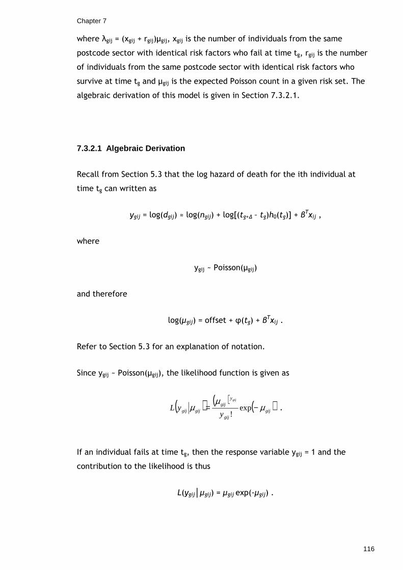
Chapter 7
116
where λgij = (xgij + rgij)µgij, xgij is the number of individuals from the same
postcode sector with identical risk factors who fail at time tg, rgij is the number
of individuals from the same postcode sector with identical risk factors who
survive at time tg and µgij is the expected Poisson count in a given risk set. The
algebraic derivation of this model is given in Section 7.3.2.1.
7.3.2.1 Algebraic Derivation
Recall from Section 5.3 that the log hazard of death for the ith individual at
time tg can written as
ygij = log(dgij) ≈ log(ngij) + log[(tg+∆ – tg)h0(tg)] + βTxij ,
where
ygij ~ Poisson(µgij)
and therefore
log(µgij) = offset + φ(tg) + βTxij .
Refer to Section 5.3 for an explanation of notation.
Since ygij ~ Poisson(µgij), the likelihood function is given as
( ) ( ) ( )gijgij
ygij
gijgij yyL
gij
µµ
µ −= exp!
.
If an individual fails at time tg, then the response variable ygij = 1 and the
contribution to the likelihood is thus
L(ygijµgij) = µgij exp(-µgij) .

Chapter 7
117
Otherwise, if the individual survives at time tg, then the response variable ygij =
0 and the contribution to the likelihood is then
L(ygijµgij) = exp(-µgij) .
If xgij individuals fail and rgij individuals survive (say), from the same postcode
sector and with identical risk factors, µgij will be the same for all such individuals
and hence the contribution to the total likelihood is
( ) ( ) ( ) ( )gijgijgijgijx
gijgijgij rxyL gij µµµµ −−= expexp
( ) ( )[ ]gijgijgijx
gij rxgij µµ +−= exp
( )( )[ ] ( )[ ]
!
exp!
gij
gijgijgijx
gijgijgij
xgijgij
gij
x
rxrx
rx
x gij
gij
µµ +−+
+= .
Therefore
ygij ~ Poisson(λgij) ,
where
λgij = (xgij + rgij) µgij .
Hence
log(λgij) = log[(xgij + rgij) µgij]
= log(xgij + rgij) + log(µgij) = log(xgij + rgij) + log(ngij) + φ(tg) + βTXij ,
since, as written above, and shown in Section 5.3, log(µgij) = log(ngij) + φ(tg) +
Xijβ. This is now Equation 7.2, the continuous-time hazard model to be fitted to
the aggregated dataset, and the offset term is now log(xgij + rgij) + log(ngij).

Chapter 7
118
7.3.2.2 Obtaining the Aggregated Dataset
This section gives an overview of how the aggregated dataset is created from the
original expanded dataset in MLwiN.
Before Equation 7.2 can be fitted, the original expanded dataset (Table 5.2)
must be aggregated so that, for each risk set, there is just one line of data
representing all individuals within the same postcode sector with the same
values for the covariates in a particular model. The new response variable and
the additional offset term, log(xgi + rgi) must be also be created. Note that xgi +
rgi is the total number of individuals in a cell within postcode sector at the
beginning of each risk set.
The first step in creating the aggregated dataset is to define the new level-1
units i.e. the cells within postcode sectors defined by each combination of the
chosen covariates. For each risk set (where a risk set still corresponds to each
specific event time), the number of individuals within a postcode sector with a
particular covariate combination are counted and this creates the level-1 ‘cells’,
giving the number at risk at the beginning of each risk set, i.e. xgi + rgi. If any
cells are empty, i.e. there is no-one within a particular postcode sector with a
particular covariate combination, then this cell may be omitted. Each cell within
postcode sector is given a level-1 identifier. Next, the response variable (i.e. the
number of individuals in each cell within postcode sector that are admitted
during each risk set) is created. This is done by summing the response variable
from the original expanded dataset, ygij, for all individuals in each cell within
postcode sector. This gives the number of psychiatric admissions in each risk set
for each cell within postcode sector. ngi, the number of people who fail in each
risk set across all postcode sectors, is the same as in the original Poisson model
fitted to the ungrouped continuous-time expanded dataset.
Following aggregation, the size of the original expanded dataset will be reduced;
however, as discussed in Section 7.3.1, the percentage reduction will depend on
the number of covariates being used for the grouping. Grouping on a larger
number of covariates will lead to a smaller percentage reduction in the original
expanded dataset.

Chapter 7
119
7.3.2.3 Modelling the Baseline Hazard Function
Several forms are available for the baseline hazard function, φ(tg). Two common
ways of estimating φ(tg), as discussed in Section 5.3.3.3, include fitting a
polynomial function or using blocking factors. If there are a large number of
time points, as may usually be the case when time is being treated as a
continuous variable, fitting a polynomial function is the form recommended by
Yang & Goldstein [163], as it avoids the need for estimating a large number of
dummy variables, which would be the case if blocking factors were used. For a
full discussion of modelling the baseline hazard function refer to Section 5.3.3.3.
7.3.3 Discrete-Time Models
Section 7.2 discussed how discrete-time hazard models, with time intervals of
either equal or varying lengths, could be fitted as an alternative to continuous-
time hazard models using a standard logistic model. The binary responses,
indicating whether or not an individual failed in a given time period, followed a
Bernoulli(πgij) distribution. Fitting the logistic model in MLwiN still required use
of an expanded dataset with each individual having a line of data corresponding
to each risk set they survived. As time was grouped into intervals, instead of
having a risk set for each distinct failure time as in the continuous-time case,
the expanded dataset was much smaller than the original expanded continuous-
time dataset; however, it was anticipated that this already smaller expanded
dataset for fitting discrete-time hazard models could be reduced even further by
aggregating it also so that there would be just one line of data representing all
individuals within the same postcode sector with the same values of covariates
in a particular model. This would mean, however, that the response, which
would now be the proportion of individuals in a cell within postcode sector who
failed in each risk set, would no longer follow a Bernoulli distribution as the
denominator for the proportion, ngij, would no longer be 1. Instead, ngij would
now correspond to the number of individuals in a risk set for each cell within
postcode sector meaning that the responses would follow a Binomial(ngij, πgij)
distribution. The algebraic derivation of the Binomial model follows in Section
7.3.3.1.

Chapter 7
120
7.3.3.1 Algebraic Derivation
Recall from Section 7.2.2.1 that the logistic model for modelling πgij, the
probability of an individual failing in the current time period, given that they
survived from the last period is written as
( ) ( ) ijT
ggijgij
gij xtit βϕππ
π+==
−log
1log ,
where the actual binary response, ygij, is 1 if the individual fails in the current
time period, and 0 otherwise, and follows a Bernoulli(πgij) distribution (i.e. a
Binomial distribution with ngij = 1).
Therefore, the likelihood function is given as
( ) ( ) gijgij ygij
ygijgijgijyL −−= 11 πππ .
If an individual fails at time tg, the contribution to the likelihood is thus
L(ygijπgij) = πgij .
Otherwise, if the individual survives at time tg, the contribution to the likelihood
is then
L(ygijπgij) = (1 - πgij) .
If xgij individuals fail and rgij individuals survive (say), from the same postcode
sector and with identical risk factors, πgij will be the same for all such
individuals and hence the contribution to the total likelihood is
( ) ( ) ( ) gijgij rgij
xgijgijgijyL πππ −= 1
( ) ( ) gijgijgij xngij
xgij
−−= ππ 1 ,
since ngij = xgij + rgij.

Chapter 7
121
Hence
ygij ~ Binomial(ngij, πgij) .
7.3.3.2 Obtaining the Aggregated Dataset
As in Section 7.3.2.2, this section will just give a brief overview of how the
aggregated dataset is created.
As with aggregating the data for the continuous-time model in Section 7.3.2.2,
the discrete-time expanded dataset must again be rearranged so that, for each
risk set, there is just one line of data representing all individuals within the
same postcode sector with the same values for the covariates in a particular
model. To fit the discrete-time model, the new binomial-distributed observed
responses, ygij, i.e. the proportion of individuals in each cell within postcode
sector who fail within a given risk set and the denominator for the proportion,
ngij, corresponding to the number of individuals in a risk set for each cell within
postcode sector, must be created.
Similarly to Section 7.3.2.2, the first step is to define the new level 1 cells
within postcode sectors by counting, for each risk set (where this time a risk set
corresponds to a specific time interval), the number of individuals within a
postcode sector with a particular covariate combination. This also creates the
denominator for the proportion, ngij. Each cell within the postcode sector is
given a level-1 identifier and again a cell may be omitted if there is no-one in
that postcode sector with the specified covariate combination. Next, the
response variable, ygij, is created using the ungrouped discrete-time expanded
dataset. Because, in the ungrouped discrete-time expanded dataset, each
individual in a given postcode sector has a binary response taking the value ‘1’ if
the individual fails in a given time interval and the value ‘0’ otherwise, the
proportion of individuals who fail in a given time interval for each cell within
postcode sector (i.e. the new response in the aggregated dataset) can be
calculated by summing the values of the binary response variables at time tg for
all individuals within a particular cell within postcode sector, and dividing it by

Chapter 7
122
the number of individuals in that cell within postcode sector (at time tg). For
example, suppose that at time tg there are 4 individuals in a given cell within
postcode sector with binary responses (0, 0, 1, 0), i.e. one person in this cell
within postcode sector fails during this particular time interval (time tg).
Therefore, the proportion of individuals in this cell within postcode sector who
fail at this particular time is (0 + 0 + 1 + 0)/4 = 1/4, which is the new response,
ygij, in the aggregated discrete-time dataset.
7.3.3.3 Modelling the Baseline Hazard Function
In the case of discrete-time models, where time is grouped into intervals,
blocking factors would be an appealing choice for modelling the baseline hazard
function, φ(tg). There would be a blocking factor for each time interval.
However, this choice may not be desirable if there are a lot of time intervals,
and hence a continuous polynomial function may be used instead. A full
discussion of this can be found in Section 5.3.3.3.
7.3.3.4 Determining the Length of Time Intervals
As discussed in Section 7.2.2.2, time intervals can either be constructed
corresponding to when events occur, thus giving time intervals of varying length,
or time can be divided into predetermined intervals, such as calendar years.
Fewer time intervals will mean a greater percentage reduction in the size of the
expanded dataset.
7.3.3.5 Estimation
Procedures for estimating non-linear models are discussed in Section 5.3.5.

Chapter 7
123
7.4 Bayesian Survival Models
7.4.1 Introduction to Bayesian Multilevel Survival Models
To recap, interest in the Scottish Health Survey data involved investigating the
association between psychosocial distress, as determined by the GHQ-12 and
time until first psychiatric hospital admission in Scotland, which was measured in
days from Scottish Health Survey interview. Previously, a multilevel Cox
proportional hazards model was fitted via a Poisson model in MLwiN, and
parameters were estimated using first-order penalised quasi-likelihood (PQL).
This model may also be fitted using a Bayesian approach and estimated using
Markov chain Monte Carlo (MCMC). However, as discussed in Section 5.3.3.2, the
data must be rearranged so that each individual has a line of data corresponding
to each risk set they survived before the Poisson models can be fitted. This can
lead to a vast increase in the size of this new expanded dataset, especially if the
size of the original dataset before expansion is already large, meaning that
models will take a long time to run when MCMC methods of estimation are used,
and certainly longer than when PQL methods are used. However, there are
advantages in using a Bayesian approach over a frequentist approach, especially
for random-effects models due to the connection between them and Bayesian
hierarchical models, and of using MCMC methods of estimation over maximum
likelihood methods. These advantages will be briefly considered here.
One of the main advantages of using a Bayesian approach over a frequentist
approach is that, in addition to the sampling distribution, P(xθ), it allows any
prior knowledge about the value of θ (obtained, for example, through previous
experiments or research), where θ represents some quantity of interest, to be
incorporated into analysis as a probability density function, P(θ).
Given these two distributions, the joint distribution of (θ, x) can be constructed
as follows:
P(θ, x) = P(xθ)P(θ).
The likelihood function, P(xθ), provides the chances of each value of θ having
led to the observed value of x and the prior density contains the probability

Chapter 7
124
distribution of θ before observation of the data, x [210]. However, observing the
data changes the information about a parameter, and therefore inference should
be based on the probability distribution of θ after observing the data. This
distribution is known as the posterior distribution, and can be obtained via
Bayes’ Theorem:
( ) ( ) ( )( )xP
PxPxP
θθθ =
( ) ( )θθ PxP∝ .
where
P(x) = ∫ P(xθ)P(θ) dθ .
Equation 7.3
A ‘drawback’ of the Bayesian approach, especially for non-linear models such as
the proportional hazards model, is that the likelihood function does not have an
analytical form, and there can be difficulty integrating the required integrals.
Previously, numerical integration or analytical approximation techniques would
be required for parameter estimation in such models; however, with the recent
advances in computing technology, techniques such as Markov Chain Monte Carlo
(MCMC) may be used as an alternative to traditional approaches. MCMC will be
discussed further in section 7.4.5.1.
Bayesian inference using MCMC methods has several advantages over frequentist
approaches. Firstly, unlike the frequentist approach, which relies heavily on
asymptotic approximation and can raise the issue of whether the sample size is
large enough for these approximations to be valid, Bayesian inference allows
exact inference for any sample size [211]. Secondly, Bayesian inference using
MCMC allows more complex models to be fitted straightforwardly. For a
thorough comparison of Bayesian and likelihood-based methods for fitting
multilevel models, refer to Browne & Draper [212].
Although there is a large amount of literature available on the proportional
hazards model, very little of this involves Bayesian inference [213]. This has
mainly been because of computational limitations; however, as discussed above,
MCMC methods, which are now much more accessible using packages such as

Chapter 7
125
WinBUGS, make estimation of previously intractable models more
straightforward.
It was discussed above that, although the Poisson model fitted in MLwiN could be
fitted using a Bayesian approach and MCMC methods of estimation; MCMC
methods would prove to be very slow because of the large person-period dataset
required to fit the Poisson model. However, as an alternative, WinBUGS allows
frailty models to be fitted to multilevel survival data. As the frailty modelling
approach does not require any data expansion, estimation of these models may
be faster. Frailty models are discussed in Section 7.4.2. For a brief review of
previous research on frailty modelling from both a frequentist and a Bayesian
viewpoint, refer to Sargent [214].
7.4.2 Frailty Models
7.4.2.1 Introduction to Frailty Models
The term ‘frailty’ was originally suggested by Vaupel et al. [215] in the case of
univariate survival data and by Clayton [216] for bivariate data. For univariate
data, the frailty is a random effect used to represent unobserved population
heterogeneity among individuals, i.e. the influence of unobserved or
unmeasurable risk factors, in univariate survival analysis [217-219]. Clayton
[216], on the other hand, studied pairs of related individuals (e.g. fathers and
sons), and included a parameter to measure the association arising when two
members of a pair share some common influence. More recently, frailty models
have also become popular for modelling multivariate survival data. Multivariate
survival data may also be referred to as ‘correlated survival data’ or ‘clustered
data’ [161]. There are two ways in which survival times may be
correlated/clustered (note that these terms will be used interchangeably
throughout the thesis). Firstly, observations may be clustered in a way that
introduces an association between the individual survival times within a cluster;
for example, individuals within a postcode sector, as in the Scottish Health
Survey, may have some unmeasured environmental factors in common [220,
221]. Secondly, if several events are measured on the same person (recurrent

Chapter 7
126
event data) then correlation between events within an individual would be
expected [220]. In the case of multivariate survival data, the frailty represents
an unobserved random effect shared by individuals within a cluster [160]. Frailty
models are mixed models or random effects models for survival data where the
frailty variable, assumed to act multiplicatively on the hazard function, models
the dependence between survival times [222-224]. The frailty term allows
individuals in the same cluster to share a common baseline hazard function, but
allows this hazard function to differ between clusters [214]. Because the frailties
act multiplicatively on the baseline hazard, they are interpreted as relative
risks. The most common type of frailty model for modelling correlated survival
data is the so-called ‘shared frailty model’. The shared frailty model will be
discussed in Section 7.4.3.
7.4.3 The Shared Frailty Model
The shared frailty model is a conditional independence model in the sense that
event times of individuals within a cluster are independent, conditional on the
frailty terms [161, 220]. The model assumes two sources of variation – the group
variation, which is described by the frailty, and individual random variation,
which is described by the hazard function [161].
The hazard at time t, conditional on the frailty, w, is assumed to be the product
of the frailty and a baseline hazard, h0(t), such that
h(tw) = wh0(t) .
The shared frailty model is, in fact, an extension of the proportional hazards
model therefore allowing covariates to be incorporated into the model. Thus,
the hazard function at time tij, where Tij is the survival (failure) time of the ith
subject (i = 1, . . . , n) in the jth cluster (j = 1, . . . , m), given the unobserved
frailty parameter, wj, and fixed observed covariate vector, xij (which may be
time dependent), is
h(tijxij, wj) = h0(tij)exp(βTxij) wj .

Chapter 7
127
The frailty random variables, wj, are assumed to be independent and identically
distributed for each cluster, and typically follow some parametric distribution
with unit mean and unknown variance, σw2. Any positive distribution can be
chosen to model frailty [225]. However, there are some common choices in the
literature which will be considered in Section 7.4.3.1. The mean is constrained
to be one in order to make the baseline hazard function identifiable. The
baseline hazard function can then be interpreted as the hazard rate of an
‘average individual’ [226]. Thus, individuals with frailty greater than one have
an increased hazard of failure and vice versa. The unknown variance parameter,
σw2, measures the between-cluster variation. A variance of zero implies that
individuals within the same cluster are independent, whereas a larger variance
means greater variability in frailty between clusters i.e. a greater correlation of
survival times of individuals within the same cluster [224].
Because the shared frailty model is an extension of the proportional hazards
model, there is flexibility in modelling the baseline hazard function. Shared
frailty models may be parametric, where both the frailty and baseline hazard
function follow some (positive) parametric distribution; or semi-parametric,
where a parametric distribution is specified for the frailty only and the baseline
hazard function is left completely unspecified. Various approaches to modelling
the baseline hazard function, as well as advantages and disadvantages with
following a particular approach, are discussed in section 7.4.3.2.
7.4.3.1 Choice of Frailty Distribution
This section provides a brief review of some possible choices for the frailty
distribution. A more comprehensive review of possible parametric choices can be
found in Hougaard [161] and Ibrahim et al. [221].
The conventional distribution for modelling the frailty term is the gamma
distribution [161, 218, 224, 225, 227-229]. The most common reason for using
the gamma distribution, as described in the literature, is its mathematical
convenience. This is due to the simplicity of the derivative of the Laplace
transform, meaning that traditional maximum likelihood procedures can be used

Chapter 7
128
for parameter estimation [161, 225]. Its flexible shape is another reason given
for selection of the gamma distribution as the frailty distribution [228, 229].
Although it may be the most commonly used frailty distribution for the
mathematical reasons here described, Hougaard [218] emphasised that there are
no biological reasons for choosing the gamma distribution. There are, however,
some disadvantages of the gamma distribution. Clayton [230] described that the
marginal relationship between the hazard and covariates does not follow the
proportional hazards model, and that there is a convergence of hazards. Instead,
the positive stable distribution has been recommended as an alternative frailty
distribution as it avoids this problem [161, 230]; however, as noted by Hougaard
[161], the derivatives of the Laplace transform are more complicated than with
the gamma distribution, making parameter estimation more complicated.
However, Bayesian methods using MCMC estimation can offer an alternative to
traditional frequentist methods of estimation [221]. Bayesian methods of
estimation will be discussed in Section 7.4.5.
The log-normal distribution has also been used and recommended by some
authors as the frailty distribution [161, 214, 220, 222, 225, 226, 228, 231-233]. If
uj (j = 1 , . . . , m) follows a normal distribution, where the frailty variable is
defined as wj = exp(uj), then wj follows a log-normal distribution. However,
unlike the mathematically attractive gamma distribution, where an explicit
representation of the likelihood function is always available [225], a closed-form
expression for the observed data likelihood is not allowed by the log-normal
distribution [226]. This means that more sophisticated methods of estimation
must be used. If a frequentist estimation approach is being used then the
Laplace transform and its derivatives can be approximated ([161, 233] for a
summary of frequentist methods); however, Bayesian MCMC methods may be
applied (see Section 7.4.5).
Although this section has so far discussed how it is customary for the frailty
random effect to follow some parametric distribution, a small number of authors
have, in fact, considered a nonparametric frailty distribution [234-236]. It has
been argued that misspecification of the random effects (where random effects
are defined to be the logarithms of the frailties) could lead to poor estimates of
the parameter of interest. When the frailty distribution or random effects
distribution is modelled nonparametrically, the distribution is left completely

Chapter 7
129
unspecified, with the only assumption being that it is finite [236]. Naskar [236]
adopted a semiparametric model in that the hazard function was modelled
parametrically with the distribution of the frailty being modelled
nonparametrically using a Dirichlet process. Dos Santos et al. [234] also adopted
a semiparametric approach with a parametric hazard and nonparametric frailty;
however, they did advise that a fully nonparametric approach (i.e.
nonparametric hazard and frailty) would be preferred, but that this approach is
limited by computational limitations and identifiability problems. Since then,
however, Walker & Mallick [235] did manage to adopt a fully nonparametric
approach by leaving the baseline hazard function completely unspecified, and
using Pólya trees as a Bayesian nonparametric prior for the random effects
distribution. Bayesian MCMC methods were used to overcome computational
limitations, and they argued that the identifiability problem was solved using
Pólya trees. Pólya tree distributions are generalisations of Dirichlet processes
[237]. Detailed information on Pólya trees can be found in Lavine [237, 238] and
Mauldin et al. [239].
It has been argued that the choice of frailty distribution may be relatively
unimportant [217, 223, 228, 231, 233, 240]. In particular, Sastry [228] reported
that results were ‘unlikely to be sensitive to the choice of frailty distributions
when the proportion of the population surviving the period of analysis is high,
unless the variance of the frailty distribution is large’. However, Hougaard [161]
argued that the choice of frailty distribution depends on the problem, and that
model properties of each distribution should be considered as relevant. With this
in mind, Hougaard [161, 218] compared the properties and the fit of some
commonly used frailty distributions.
7.4.3.2 Modelling the Baseline Hazard Function
Section 5.2 described how the baseline hazard function of the proportional
hazards model can be modelled either parametrically or non-parametrically. As
discussed throughout this section, the shared frailty model is an extension of the
proportional hazards model in that, conditional on the frailty, event times follow
the usual proportional hazards model. This implies that the baseline hazard

Chapter 7
130
function may be modelled nonparametrically or parametrically. In terms of
modelling the baseline hazard function parametrically, Hougaard [161]
acknowledged the Weibull model as the most natural choice of parametric
distribution as it allows for the proportional hazards model and the accelerated
lifetime model. The Weibull model will be discussed further in Section 7.4.4 as
the modelling strategy used by WinBUGS to fit the shared frailty model involves
fitting an additive frailty model with Weibull hazard.
Although the baseline hazard function may be modelled parametrically, some
have argued that the parameters of the frailty distribution may be sensitive to
the choice of distribution for the hazard, and that the choice of distribution for
the hazard may, in fact, be more important than the choice of frailty
distribution [223, 234]. On account of this argument, it may be better to model
the baseline hazard function nonparametrically and leave it completely
unspecified. This would mean adopting a semiparametric approach if the frailty
follows some parametric distribution, as is usually the case, or a fully
nonparametric approach if the frailty is also being modelled nonparametrically
(see Section 7.4.3.1). A nonparametric distribution for the hazard function has
been used by Klein [241] in a frequentist framework and by Clayton [230] in a
Bayesian framework. Sinha & Dey [242] also considered different ways of
Bayesian modelling for nonparametric parts of the frailty model, such as the
baseline hazard function.
7.4.4 Fitting Frailty Models in WinBUGS
Section 7.4.1 remarked that multilevel survival models using a Bayesian
framework could be fitted in packages such as WinBUGS. WinBUGS, an acronym
for ‘Bayesian Analysis Using Gibbs Sampling’ aims to make practical MCMC
methods available to applied statisticians and is an ideal package to use as it can
be downloaded free of charge from http://www.mrc-
bsu.cam.ac.uk/bugs/winbugs/contents.shtml, making its use readily available.
WinBUGS 1.4 is the current (Windows) version of the package it and can be
readily applied to implement the shared frailty model. To fit the frailty model,
WinBUGS assumes a parametric Weibull distribution for the survivor function.

Chapter 7
131
Suppose that (r, γ) are the parameters of the Weibull distribution. Then the
hazard function is given by
h(tijxij, wj) = γrwitijr-1exp(βTxij).
This model is a multiplicative frailty model; however, the modelling strategy
adopted in WinBUGS is based on an additive frailty model. The additive frailty
model is achieved by writing
h(tijxij, uj) = µijrtijr-1,
Equation 7.4
where
log(µij) = α + βTxij + uj.
Exponentiating this leads to the parameterisation
tij ~ Weibull(r, µij),
for i = 1, . . . , n and j = 1, . . . , m. The shape and scale parameters of the
Weibull distribution are denoted by r and µij respectively. The shape parameter,
r, allows the hazard function to increase or decrease with increasing time, and is
interpreted as follows: for r < 1 the hazard rate strictly decreases in a nonlinear
pattern as time increases; for r = 1 the hazard rate is constant (and the Weibull
and exponential survival probabilities are the same); and, for r >1, the hazard
rate is strictly increasing in a nonlinear pattern as time increases [243].The uj’s
are the additive random effects in the exponent of the hazard model and are
assumed to follow a normal (0, τ) distribution. In fact, the additive frailty model
is actually a multiplicative frailty model with a log-normal frailty distribution;
therefore, the additive and multiplicative frailty models should yield similar
inferences [221, 244].

Chapter 7
132
7.4.4.1 Fitting the Weibull Model to the Scottish H ealth Survey Data
The association between the GHQ-12 and the hazard of first psychiatric hospital
admission in Scotland can be investigated using frailty models, which were fitted
in WinBUGS via a Weibull model with a log-normal frailty distribution.
Recall that the SHeS dataset consisted of 15305 individuals within 624 postcode
sectors; therefore, the model is given by
tij ~ Weibull(r, µij),
for i = 1, . . . , 15305 and j = 1, . . . , 624. Thus, if taking a GHQ-12 score of 0 as
the baseline, the model is written in WinBUGS as follows:
The ui’s are the additive random effects for postcode sectors in the exponent of
the hazard model and are assumed to follow a normal (0, σu2) distribution. In
WinBUGS, the variance of the normal distribution is written in terms of the
precision, τ, where τ = 1/ σu2.
In line 5 of the above WinBUGS code, it can be seen that the distribution for
time is expressed as time[i] ~ dweib(r,mu[i]) I(censor[i],). This indicates that,
for the censored observations, the survival distribution is a truncated Weibull
distribution, with lower bound corresponding to the censoring time [245].

Chapter 7
133
The regression coefficients, shape parameter and the random effects variance
are given non-informative priors. Choice of priors will be discussed in Section
7.4.4.2 below. Bayesian estimation of the parameters, as performed in
WinBUGS, is discussed in Section 7.4.5.
Following estimation of log(µij), the hazard function of the additive hazard
Weibull model is calculated as shown in Equation 7.4. It may also be of interest
to calculate other properties, such as the mean survival time.
If the survivor function is distributed as Weibull, then the mean survival time is
given as
E(t) = µ-1/rΓ(1 + 1/r),
where Γ represents the gamma function.
The survivor function is given as
S(t) = P(T ≥ t) = exp(-µtr).
7.4.4.2 Priors
Unlike the frequentist approach, the Bayesian approach allows any prior
knowledge about the value of θ, where θ represents some quantity of interest,
to be incorporated into analysis as a probability density function. As seen in
Equation 7.3 in Section 7.4.1, Bayes theorem can be written as
P(θx) α P(xθ)P(θ) ,
where P(θx) is the posterior distribution, P(xθ) is the likelihood function, and
P(θ) is the prior distribution. Prior distributions must be specified for all
unknown parameters in the analysis. The frailty model is a hierarchical model,
and therefore involves several levels of conditional prior distributions, where the
dependence between the θ’s is accounted for by modelling them as conditionally
independent given some hyperparameter.

Chapter 7
134
There are a number of cases in which it may not be desirable to incorporate
prior information into the analysis. Firstly, prior information on θ may not be
available; or it may be preferable to let the data dominate; or, finally, MCMC
methods may just be being used for computational convenience and hence the
inclusion of prior information may not be desired [246]. In these cases, ‘vague’
or ‘reference’ priors may be used. Vague priors are also commonly referred to as
‘diffuse’ or ‘non-informative’.
In this thesis, MCMC methods have been adopted for computational convenience
since fitting multilevel survival models via Bayesian frailty models in WinBUGS
does not require the data expansion required to fit multilevel survival models via
a Poisson model in MLwiN. With this in mind, vague priors were adopted for all
parameters and hyperparameters. In the Weibull model (code given above),
priors must be specified for the regression coefficients, βk (k = 1, 2, 3) and the
random effects, uj (j = 1 , . . , 624), as well as a hyperprior for the random
effects variance, σu2, and a prior for the shape parameter, r, of the Weibull
distribution.
It is assumed that the GHQ-12 scores in the SHeS are representative of GHQ-12
scores in the Scottish population, and therefore beta regression coefficients
were assigned independent vague Normal priors with zero mean and precision
0.0001,
βk ~ Normal(0, 0.0001), (k = 1, 2, 3).
Recall that the betas represent logarithms of relative risks.
For the shape parameter of the Weibull distribution, Spiegelhalter et al. [245]
used a Gamma(1, 0.0001) prior which is slowly decreasing on the positive real
line; however, assigning a Gamma prior to the shape parameter when fitting the
model to the SHeS dataset tended to cause ‘trap’ messages in WinBUGS. Trap
messages correspond to an error which has not been picked up by WinBUGS
[245], and generally these messages are difficult to decode, especially for novice
users. However, suggestions on how to interpret some common trap messages
are given in the WinBUGS manual [245].

Chapter 7
135
Instead, a vague log-Normal prior with mean one was assigned such that,
log(r) ~ Normal(0, 0.1) .
Finally, a prior must be specified for the random effects. By definition of the
log-Normal frailty model, it is assumed that the uj’s follow a Normal distribution
with mean zero and variance σu2. In WinBUGS, the variance is specified in terms
of the precision, τ; therefore, the prior distribution for the uj’s is
uj ~ Normal(0, τ) , (j = 1, . . . , 624).
A hyperprior must also be specified for the variance term. A vague hyperprior
will also be used for this. There are a couple of options usually adopted by
WinBUGS for this purpose. The first option is a vague Uniform prior on the
standard deviation, and the second option is a vague Gamma prior on the
precision i.e. an inverse-Gamma prior on the variance. The WinBUGS manual
advises the use of the Uniform prior on the standard deviation with use of the
Gamma prior on the precision generally not recommended as it can commonly
cause trap messages [245]. Gustafson [231] also discussed why an inverse-
Gamma prior on the variance may not be appropriate.
Therefore, the following vague hyperprior was specified for the random effects
standard deviation:
σu ~ Uniform(0, 1).
Lambert et al. [246] recommended that a sensitivity analysis should be
performed when using prior distributions that are intended to be vague for the
between-unit variance. However, they also discussed how the influence of the
prior distribution is reduced as the number of higher-level units increases. As
there are a large number of postcode sectors in the SHeS dataset (624 postcode
sectors), inferences should not be sensitive to the choice of prior distribution for
this parameter.

Chapter 7
136
7.4.5 Estimating the Parameters in WinBUGS
7.4.5.1 Markov Chain Monte Carlo
Bayesian Markov chain Monte Carlo (MCMC) methods are commonly used as
estimation procedures in shared frailty models. The posterior distribution in
hierarchical models, such as the frailty model, is usually difficult to integrate
out in order to find the marginal posterior of each random parameter [225];
however, MCMC methods can now allow analysis based on previously intractable
posterior distributions [231]. MCMC methods avoid the need for high-dimensional
integration by performing the integration implicitly through generating samples
from the joint posterior distribution of the unknown parameters [247, 248].
The general idea behind MCMC is as follows. Suppose the target distribution,
π(θ) for θ є E ⊂ Rn, where π(θ) = p(θx) (the posterior distribution) is complex
and cannot be sampled from directly. Samples from π can, however, be obtained
indirectly by constructing a Markov chain with state space E whose equilibrium
(stationary) distribution is π(θ). If the chain is run for long enough, simulated
values can thus be treated as a dependent sample from the target (posterior)
distribution which can be used to summarise characteristics of π. In order to
reach the stationary distribution, the chain must satisfy three conditions. It must
be irreducible, aperiodic and positive recurrent. Further details of this can be
found in Gilks et al. [249].
Markov chains with the desired stationary distribution are constructed using
MCMC algorithms, the two most common being the Gibbs sampler and the
Metropolis-Hastings algorithm. The Gibbs sampler is the easiest algorithm to
implement and is the algorithm adopted by WinBUGS. Therefore, only Gibbs
sampling will be discussed in this thesis (Section 7.4.5.2). However, details of
the Metropolis-Hastings algorithm can be found in Smith & Roberts [250], Brooks
& Roberts [251], Gilks et al. [249] and Gamerman & Lopes [210].

Chapter 7
137
7.4.5.2 Gibbs Sampling
This subsection will give a brief introduction to Gibbs sampling. For a more
comprehensive review refer to Gilks et al. [249] and Gamerman and Lopes [210].
The Gibbs sampler is an iterative Monte Carlo method used to generate samples
from difficult multivariate posterior distributions. It generates samples indirectly
from the joint distribution of the parameters without having to calculate the
density by repeatedly sampling from the full conditional posterior distributions
of the model parameters to produce realisations from the joint posterior
distribution. Considering only one unknown quantity at a time, the Gibbs
sampler generates a value from the corresponding full conditional distribution
given the current values of the other quantities [230]. In general, the Gibbs
sampler proceeds as follows. Suppose the parameter θ is partitioned into p
subvectors (or possibly scalars) such that
θ = θ1, θ2, . . . , θp.
If the current state of the Markov chain is
θ(t) = θ1(t), θ2
(t), . . . , θp(t),
then the Gibbs sampler proceeds to θ(t+1) in p steps as follows.
This process generates a Markov chain and, provided each conditional
distribution is sampled from sufficiently frequently, under a wide set of
conditions, the samples obtained are from the joint posterior distribution, where
θ(t) is the state vector of a convergent Markov chain with the posterior
distribution as the stationary distribution [252]. Samples obtained from the
posterior distribution can then be used for inference.

Chapter 7
138
Gilks et al. [249] considered some steps required to implement Gibbs sampling.
Firstly, they stated that starting values must be provided for all unobserved
nodes. Starting, or ‘initial’ values, as they are referred to in WinBUGS and will
be referred to in the thesis from here on, are chosen for the parameters of the
model before proceeding through the steps of the algorithm. Although WinBUGS
can generate initial values for unobserved nodes by forward sampling from the
prior distribution for each parameter [245], it is recommended that initial values
should be provided for parameters with vague prior distributions. The values
chosen for initial values are not particularly important in terms of inferences
made from Gibbs sampling since, when the chain is run for long enough to
achieve equilibrium, it loses all dependence on initial values [247, 249].
However, choice of initial values can affect the performance of the chain, for
example, the speed at which it reaches convergence. Methods adopted for the
selection of initial values have included, for example, using estimates from
simpler models by setting the hyperparameters to fixed values, or, alternatively,
using maximum likelihood estimates [247, 253]. More rigorous methods of
selection of initial values are discussed in Brooks [247] and references therein.
Construction of the full conditional distributions for each unobserved node is the
second point to be considered by Gilks et al. [249]. The full conditional
distributions are derived from the joint distribution of the variables as follows.
( ) ( )( )∫ −
−− =
iii
iiii
dθθθπθθπθθπ
,
, .
WinBUGS automatically constructs the full conditional distributions and chooses
appropriate methods for sampling from them [254]. If random variables are
Gamma, inverse-Gamma or Normally distributed, as is usually the case in frailty
models, sampling is fairly straightforward via standard algorithms. However, in
other cases, alternative random variate generating methods, such as the
‘inversion method’ or the ‘rejection method’, can be used [213]. If the full
conditional posterior distributions of the model parameters can be shown to be
log-concave, adaptive rejection sampling can be used. See Dellaportas and Smith
[213] for a definition of log-concavity, and Dellaportas and Smith and Gilks et al.

Chapter 7
139
[249] for a discussion of adaptive rejection sampling as well as alternative
methods for random variate generation.
The third point considered by Gilks et al. [249] is that of monitoring
convergence. This issue will be discussed separately in Section 7.4.6.
7.4.6 Monitoring Convergence in WinBUGS
Section 7.4.5 above discussed that, provided a Markov chain is run for long
enough during a period referred to as ‘burn-in’, simulated values can be treated
as a dependent sample from the target (posterior) distribution which can be
used to summarise characteristics of π. The purpose of the burn-in period is to
remove dependence of the simulated chain on its starting location [253] in order
for effective convergence to be reached. One of the main problems, however, is
determining the length of the burn-in period in order to safely assume that all
further samples are representative of the stationary distribution of the Markov
chain. Therefore, it is necessary to assess convergence using procedures called
‘convergence diagnostics’.
The study of convergence can be approached in two ways. The first approach is
theoretical and will not be considered here. However, a discussion of this can be
found in Cowles & Carlin [255] and Gamerman & Lopes [210] and references
therein. The second approach applies diagnostic tools to the output of the
simulation, and will be the approach considered here. Cowles & Carlin
recommended that a variety of diagnostic tools should be used to assess
convergence, and there are a number available in WinBUGS. In particular,
convergence will be assessed here by using the Gelman-Rubin method and trace
plots for each parameter. These will be reviewed in Sections 7.4.6.1 and 7.4.6.2
below. However, comprehensive reviews of further techniques for monitoring
convergence can be found in Cowles & Carlin, Brooks & Roberts [251], Gilks et
al. [249] and Gamerman & Lopes [210].
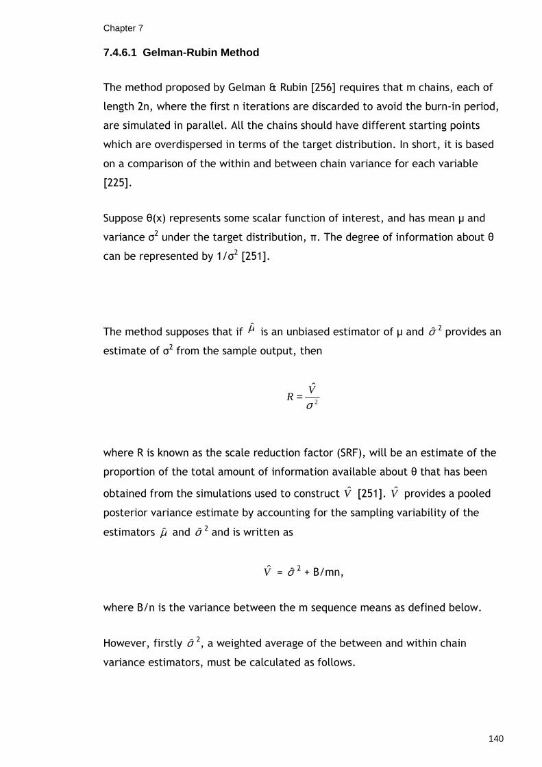
Chapter 7
140
7.4.6.1 Gelman-Rubin Method
The method proposed by Gelman & Rubin [256] requires that m chains, each of
length 2n, where the first n iterations are discarded to avoid the burn-in period,
are simulated in parallel. All the chains should have different starting points
which are overdispersed in terms of the target distribution. In short, it is based
on a comparison of the within and between chain variance for each variable
[225].
Suppose θ(x) represents some scalar function of interest, and has mean µ and
variance σ2 under the target distribution, π. The degree of information about θ
can be represented by 1/σ2 [251].
The method supposes that if µ is an unbiased estimator of µ and σ 2 provides an
estimate of σ2 from the sample output, then
2
ˆ
σV
R =
where R is known as the scale reduction factor (SRF), will be an estimate of the
proportion of the total amount of information available about θ that has been
obtained from the simulations used to construct V [251]. V provides a pooled
posterior variance estimate by accounting for the sampling variability of the
estimators µ and σ 2 and is written as
V = σ 2 + B/mn,
where B/n is the variance between the m sequence means as defined below.
However, firstly σ 2, a weighted average of the between and within chain
variance estimators, must be calculated as follows.

Chapter 7
141
To begin, define B/n as the variance between the m sequence means, θ i., each
based on n values of θ where
( )( )1
..2
.
−
−=∑
mn
B ii θθ
, (i = 1, . . . , m)
Next, W, the average of the m within-sequence variances, si2, each of which has
n-1 degrees of freedom, is defined as
W = ∑i si2/m, (i = 1, . . . , m).
σ 2 is thus calculated as
Bn
Wn
n 11ˆ 2 +−=σ .
Under stationarity, σ 2 is an unbiased estimator of σ2, but will overestimate σ2 if
the starting distribution is appropriately overdispersed. Brooks & Gelman [257]
warn that σ 2 can be too low if over-dispersion does not hold, meaning that
convergence can be falsely diagnosed.
Following calculation of σ 2, V and hence R, the scale reduction factor, can be
calculated. However, the denominator of R, σ2, is unknown, and therefore it
must be estimated from the data. W is thus used to provide an (under)estimate
of σ2, which, in turn, means R can be (over)estimated by
mn
n
Wm
m
W
VR
1ˆ1ˆˆ
2 −−+== σ .
R is referred to as the potential scale reduction factor (PSRF) and can be
interpreted as a convergence diagnostic. If the value of R is large, then σ 2 can
be decreased further by running more simulations, thereby improving inference
about the target distribution, as it is clear that the simulated sequences have
not yet made a full tour of the target distribution [257]. However, if R is close
to 1, then it can be concluded that each of the m sets of n simulated
observations is close to the target distribution [257].

Chapter 7
142
The PSRF can be modified to account for sampling variability in the variance
estimates by using the correction factor (d+3)/(d+1). Justification of this
correction factor can be found in Gelman & Rubin [256] and Brooks & Gelman
[257].
Using this correction factor gives the corrected scale reduction factor (CSRF),
which is defined as
W
V
d
dR
d
dRc
ˆ
)1(
)3(ˆ)1(
)3(ˆ++=
++= .
Interpretation of R c is the same as that for R . It is usually taken to assume that
convergence has been reached if R c < 1.2 for all parameters [257].
This original method was further developed by Brooks & Gelman [257] so that
more than one parameter could be considered simultaneously. In that case, θ
denotes a vector of parameters. Further details of this can be found in Brooks &
Gelman and Brooks & Roberts [251].
The CSRF provides a useful indicator as to whether or not convergence has been
attained; however, Brooks & Gelman [257] argued that monitoring R c alone only
considers one of the three conditions which should hold at convergence. At
convergence, as well as R c approaching 1, the other conditions to hold are that
the mixture-of-sequences variance, V, should stabilise as a function of n and the
within-sequence variance, W, should stabilise as a function of n [257]. They
considered an alternative graphical approach to monitoring convergence by
dividing the m sequences into batches of length b, and then calculating V(k),
W(k) and R c(k) based on the second half of the observations of a sequence of
length 2kb (k = 1, . . . , n/b) for some suitably large n [257]. Then, as well as
plotting R c(k) against k, the two scale factors, V1/2(k) and W1/2(K), functions of k
can be included on the same plot. Both plots stabilising at the same value
indicates that convergence has been attained. Brooks & Gelman [257] noted that
the scale factors are given to the power 1/2 in order to be on a directly
interpretable scale.

Chapter 7
143
WinBUGS allows R c(k) and the two scale factors to be plotted together. A red
line is used to indicate R c(k), a green line indicates the width of the central 80%
interval of the pooled runs, and a blue line indicates the average width of the
80% intervals within the individual runs [245]. As discussed above, convergence
is attained when R c (red line) approaches 1 and the pooled and within interval
widths (green and blue lines respectively) stabilise at the same value.
Spiegelhalter et al. [245] noted that the pooled and within-interval widths are
normalised to have an overall maximum of one for plotting purposes. These plots
will be used to monitor convergence when fitting the frailty models along with
trace plots for each parameter. Refer to Section 7.4.6.2 for a discussion of trace
plots.
Although the Gelman-Rubin method requires multiple sequences to be run in
parallel using a range of different starting values, Jackman [252] noted that
some authors prefer one long run of a MCMC sampler rather than several shorter
ones, especially in a situation where convergence is slow (refer to Brooks [247]
for a further discussion). However, given improvements in computational power,
it is now usually recommended that ‘more is better’ [252]. Indeed, there are a
number of advantages in running multiple chains, as problems that would
otherwise not be revealed if only one chain was being run, such as poor mixing,
can be revealed [253].
7.4.6.2 Trace Plots
As discussed previously, Cowles & Carlin [255] recommended that a variety of
diagnostic tools should be used to assess convergence. In addition to more
formal techniques, such as the Gelman-Rubin method, ‘trace plots’ may also be
used to assess convergence for each parameter of interest. Trace plots, which
are easily attained in WinBUGS, display the iterative history of MCMC sequences
by plotting the sample values versus iteration number to try and assess when the
simulation appears to have stabilised. If running only one chain, on graphical
inspection the chain should be fairly stable around a sample value, and the trace
should be ‘caterpillar-like’ in appearance if convergence is reasonable. If more

Chapter 7
144
than one chain is being run simultaneously, in addition to the conditions which
indicate convergence when only one chain is run, the multiple chains, which
WinBUGS plots in different colours, should be overlapping each other. If this is
not the case, and the chains do not appear to be ‘mixing’ well, where mixing
refers to the degree to which a simulated chain spans the entire parameter
space [253], then a bigger burn-in period may be required.
7.4.6.3 Iterations After Convergence
Once convergence has been attained, it is necessary to run the simulation for
further iterations in order to obtain the samples to be used for posterior
inference. Although the accuracy of the posterior estimates will improve as the
number of samples saved increases, running too many further iterations will not
be computationally efficient. Therefore, Spiegelhalter et al. [245] have
suggested a way in which the accuracy of the posterior estimates may be
assessed. For each parameter, this is done by calculating an estimate of the
difference between the mean of the sampled values, which is being used as an
estimate of the posterior mean, and the true posterior mean to give what is
referred to as the ‘Monte Carlo error’ (MC error).
Spiegelhalter et al. [245] recommended that, as a rule of thumb, the simulation
should be run until the Monte Carlo error for each parameter of interest is less
than around 5% of the sample standard deviation (SD). Both the MC error and SD
are reported in the summary statistics table produced by WinBUGS.

145
8 Fitting Alternative Methods to the Scottish
Dataset: Results
This section presents results obtained from fitting the three methods described
in Chapter 7 to the Scottish Health Survey dataset.
8.1 Defining Different Risk Sets
The first alternative to be considered involved defining different risk sets.
Instead of having a risk set for each failure time as in continuous-time hazard
models, which, in the context of the Scottish Health Survey data, was the time
at which an individual was admitted to psychiatric facilities as measured in days
from survey interview, the time scale is divided into short intervals, and failures
are observed within each interval. As reviewed in Section 7.2, the data were
expanded so that each individual had a line of data corresponding to each risk
set they survived. Discrete-time hazard models were fitted with a binary
response coded as 1 if an individual was admitted to psychiatric facilities in the
time period, and 0 otherwise. Censoring was as in the continuous-time hazard
models (Section 5.4.1). As individuals were nested within postcode sectors, a
random effect for postcode sector was incorporated into the model to account
for the hierarchical structure.
For both the 1995 and 1998 surveys, follow-up time was measured from the date
of survey interview until 2004. Instead of treating time as continuous and
observing it in days, it may also seem natural to group follow-up time into years.
Grouping time into yearly intervals implied that there were fewer risk sets and
hence the size of the expanded dataset was reduced. Although grouping time
into yearly intervals led to a reduction in the size of the expanded dataset, it
was also of interest to investigate whether it was possible to establish a more
effective way of grouping time in order to reduce the size of the expanded
dataset further. To do this, time intervals were defined so that they
corresponded to times when events occurred, and thus the length of each
discrete time interval varied. The time intervals were constructed in such a way

Chapter 8
146
that the size of the expanded dataset was reduced as much as possible with a
minimal loss of information.
Sections 8.1.1 and 8.1.2 present results obtained from fitting two-level discrete-
time hazard models in MLwiN for when time intervals were grouped into years
and were of varying length respectively. Models were re-run including all
available risk factors in order to investigate if significant variables and
parameter estimates in the final discrete-time hazard models were comparable
to those obtained when fitting continuous-time hazard models (Section 5.4). The
modelling strategy employed when fitting the discrete-time hazard models was
identical to that when fitting the continuous-time models in that three separate
models were fitted. To recap, the three models included a model with GHQ-12
score only as a way of investigating the association between GHQ-12 score and
the hazard of first psychiatric admission, a model adjusting for all significant risk
factors apart from self-assessed general health and, finally, a model adjusting
for all significant risk factors including self-assessed general health as a
potential risk factor. For further information on the modelling strategy see
Section 5.4.1, and for further information on the relationship between GHQ-12
score and self-assessed general health see Section 3.2.1.2.
8.1.1 Multilevel Discrete-Time Models with Equal In tervals of Time
Table 8.2 displays results obtained from fitting discrete-time hazard models with
year-long time intervals. In order to make results obtained from fitting discrete-
time hazard models comparable with results obtained from fitting the
continuous-time hazard models (Table 5.3), first-order PQL was used to estimate
the parameters. A discussion of estimation procedures in MLwiN for non-linear
models can be found in Section 5.3.5. It should be noted again that results are
for those respondents with no psychiatric admissions prior to survey interview.
The last observation (which was censored) occurred at 3476 days from survey
interview suggesting ten year-long intervals; however, as the last event
(admission) occurred at 3046 days from survey interview, the data were
restructured into nine risk sets, with all ‘survivors’ being censored after this

Chapter 8
147
time. An example of the expanded dataset obtained in MLwiN for the first
individual is displayed in Table 8.1 below.
Table 8.1 - Expanded dataset with equal discrete ti me intervals ID Response Failure Risk Set
Indicator
Survival
Time
Number at
Risk
1
1
1
1
1
1
1
1
1
.
.
.
0
0
0
0
0
0
0
0
0
.
.
.
25
24
19
23
16
16
8
4
2
.
.
.
1
2
3
4
5
6
7
8
9
.
.
.
1
2
3
4
5
6
7
8
9
.
.
.
15208
15093
14971
14846
14453
6974
6924
6860
550
.
.
.
Size of dataset = 110643
As shown in Table 8.1, grouping time into year-long intervals reduced the size of
the expanded continuous-time dataset (Table 5.2) from just fewer than 1.9
million observations within individuals to just fewer than 111000 observations
within subjects. This was a reduction of approximately ninety four percent.
A two-level discrete-time model with a fourth-order polynomial describing the
underlying hazard was fitted in MLwiN. The logit link was used to model the
hazard. Note that results obtained here will be compared with results obtained
from fitting the continuous-time proportional hazards models (models B1, B2 and
B3) displayed in Table 5.3.

Chapter 8
148
Table 8.2 - Results from ML discrete-time models wi th equal intervals Model C1 Model C2 Model C3 Estimate(s.e) Estimate(s.e) Estimate(s.e) Fixed
Intercept (β0) -7.059(0.911) -7.536(0.939) -7.667(0.943)
tij (α1) 0.214(1.188) 0.154(0.170) 0.056(1.170) t ij
2 (α2) -0.147(0.484) -0.117(0.476) -0.071(0.476) t ij
3 (α3) 0.029(0.076) 0.024(0.075) 0.016(0.075) t ij
4 (α4) -0.002(0.004) -0.002(0.004) -0.001(0.004)
GHQ-12 Score 0 0.000** 0.000** 0.000* 1-2 (β1) 0.698(0.226) 0.571(0.227) 0.482(0.229) 3-4 (β2) 0.962(0.278) 0.674(0.282) 0.530(0.286) 5-12 (β3) 1.351(0.218) 0.943(0.226) 0.707(0.236)
Sex Male 0.000 0.000 Female (β4) -0.145(0.186) -0.105(0.187)
Age 16-24 0.000 0.000 25-34 (β5) -0.276(0.286) -0.246(0.287) 35-44 (β6) 0.005(0.277) 0.044(0.279) 45-54 (β7) -0.642(0.333) -0.694(0.335) 55-64 (β8) -0.210(0.303) -0.318(0.308) 65-74 (β9) 0.123(0.385) 0.162(0.387)
Marital Status Married/cohabiting 0.000 0.000 Other (β10) 0.478(0.179) 0.395(0.181)
Receipts of Benefits No 0.000 0.000 Yes (β11) 0.799(0.200) 0.600(0.209)
Smoking Status Non-Smoker 0.000 0.000 Current Smoker (β12) 0.810(0.213) 0.718(0.215) Ex-Smoker (β13) 0.036(0.300) 0.016(0.301)
Employment Status Full-Time 0.000 0.000 Unemployed (β14) 0.427(0.262) 0.545(0.267) Part-Time (β15) -0.364(0.253) -0.315(0.254)
Self-Assessed Health Very Good 0.000 Good (β16) 0.512(0.225) Fair (β17) 0.973(0.250) Bad (β18) 0.206(0.552) Very Bad (β19) 1.932(0.457)

Chapter 8
149
Random
Area Variation(σu2) 0.245(0.263) 0.191(0.249) 0.233(0.246)
ICC 0.069 0.055 0.066
* ptrend < 0.05 ** ptrend <0.001
Model C1 demonstrated a highly significant increasing trend in the hazard of first
psychiatric admission following survey interview (p <0.001) as GHQ-12 score
increased. Taking the anti-logit of the intercept revealed that, after adjusting
for GHQ-12, the probability of psychiatric admission in the average postcode
sector was 0.000859. The intraclass correlation (ICC = 0.069) indicated that 6.9%
of the total variation was attributable to the level of postcode sector. Parameter
estimates obtained for the fixed effects in model C1 were very similar to those
obtained in model B1. There were slight differences in the estimates of the
random effects between models C1 and B1. The postcode sector variation was
underestimated using the discrete-time model (C1) compared to the Poisson
model (B1). However, when fitting discrete-time models the response follows a
Binomial distribution, as opposed to continuous-time models where the response
is Poisson-distributed. As a result, these models and hence parameter estimates,
are not strictly comparable. It can be observed, however, that the 95%
confidence interval (not displayed here) for the higher-level variance in model
B1 contained the value of the estimate obtained in model C1.
Model C2 allowed for the adjustment of all significant risk factors apart from
self-assessed general health. The increasing trend in the hazard of admission as
GHQ-12 score increased remained highly significant following adjustment for all
significant risk factors. In addition to having a GHQ-12 score of 1 or more, other
significant risk factors associated with an increased hazard of admission included
not being married (i.e. single, separated, divorced or widowed), being in receipt
of benefits and being a current smoker. Neither of the area-level risk factors was
significantly associated with the outcome, and thus model C2 contained
individual-level risk factors only. The intraclass correlation decreased to 5.5% as
a result of adjusting for further significant demographic, socioeconomic and
lifestyle risk factors, with 22% of the total unexplained variation between

Chapter 8
150
postcode sectors being attributed to going from model C1 to model C2. Model
C2 is identical to model B2 in terms of risk factors significantly associated with
an increased hazard of psychiatric admission. Comparing model C2 to model B2
also revealed that the parameter estimates obtained for the fixed effects were
very similar for the two models. However, the postcode sector variation was
underestimated. Reasons for this difference were discussed above.
The final model (model C3) allowed for adjustment of all significant risk factors
including self-assessed general health. As in previous models (A3 and B3), the
relationship between GHQ-12 score and psychiatric admission was attenuated
following the inclusion of self-assessed general health; however, the increasing
trend in the hazard of psychiatric admission remained significant. Parameter
estimates for the fixed and random effects in model C3 were comparable to
those obtained in model B3, with the same risk factors being associated with an
increased hazard of psychiatric admission in the two models. In addition to a
GHQ-12 score of one or more, these included not being married (i.e. single,
separated, divorced or widowed), being in receipt of benefits, being a current
smoker, being unemployed and having a self-assessed general health rating other
than ‘very good’ (i.e. ‘good’, ‘fair’, ‘bad’ or ‘very bad’). As in model B3, the
between-postcode sector variation in model C3 (σu2 = 0.233) had increased as a
result of including self-assessed general health in the model; however, the
discrete-time model was still underestimating this parameter.
8.1.2 Multilevel Discrete-Time Models with Varied I ntervals of
Time
It was discussed above that time intervals should be constructed in such a way as
to reduce the size of the expanded dataset to the greatest extent possible whilst
retaining as much information as possible. Therefore, as an alternative to fitting
strict year-long time intervals, the lengths of the intervals were allowed to vary
according to when admissions occurred. Time was divided into five intervals
which were defined as shown in Table 8.3 below.
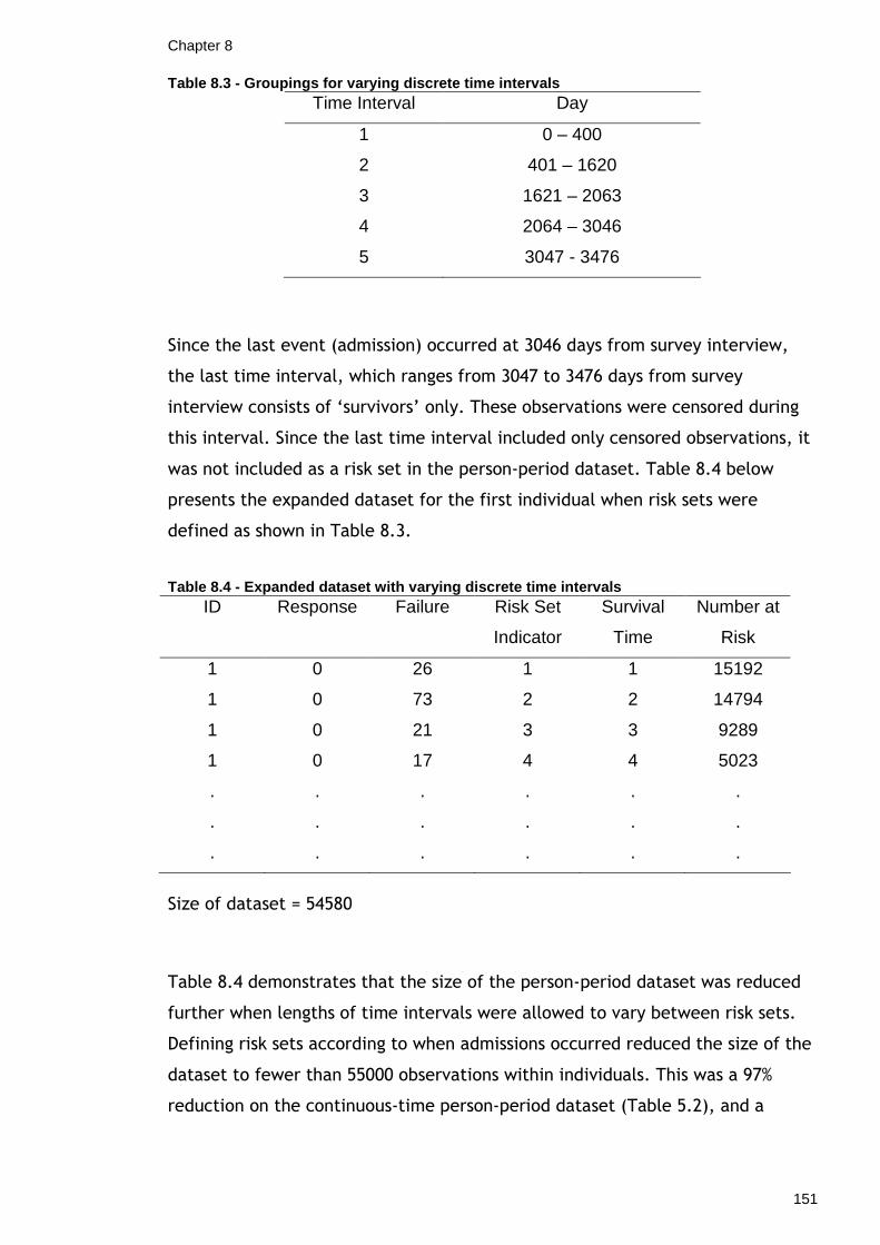
Chapter 8
151
Table 8.3 - Groupings for varying discrete time int ervals Time Interval Day
1
2
3
4
5
0 – 400
401 – 1620
1621 – 2063
2064 – 3046
3047 - 3476
Since the last event (admission) occurred at 3046 days from survey interview,
the last time interval, which ranges from 3047 to 3476 days from survey
interview consists of ‘survivors’ only. These observations were censored during
this interval. Since the last time interval included only censored observations, it
was not included as a risk set in the person-period dataset. Table 8.4 below
presents the expanded dataset for the first individual when risk sets were
defined as shown in Table 8.3.
Table 8.4 - Expanded dataset with varying discrete time intervals ID Response Failure Risk Set
Indicator
Survival
Time
Number at
Risk
1
1
1
1
.
.
.
0
0
0
0
.
.
.
26
73
21
17
.
.
.
1
2
3
4
.
.
.
1
2
3
4
.
.
.
15192
14794
9289
5023
.
.
.
Size of dataset = 54580
Table 8.4 demonstrates that the size of the person-period dataset was reduced
further when lengths of time intervals were allowed to vary between risk sets.
Defining risk sets according to when admissions occurred reduced the size of the
dataset to fewer than 55000 observations within individuals. This was a 97%
reduction on the continuous-time person-period dataset (Table 5.2), and a

Chapter 8
152
reduction of more than half (51%) on the expanded dataset when time was
grouped into year-long intervals (Table 8.1).
A two-level discrete-time model using a logit link to model the hazard was fitted
in MLwiN. As there were only four risk sets, dummy variables known as ‘blocking
factors’ were used for the modelled time intervals, with the first risk set being
taken as the baseline. As in models C1, C2 and C3 above, results obtained here
were compared with those obtained from fitting continuous-time hazard models
(models B1, B2 B3) as displayed in Table 5.3.
Results from model D1 indicated a highly significant increasing trend in the
hazard of first psychiatric admission during follow-up as GHQ-12 score increased
(p<0.001). Parameter estimates obtained for the fixed effects (GHQ-12 score)
were very similar to those obtained in model B1 and also in model C1. However,
postcode sector variation in model D1 (σu2 = 0.279) was slightly larger than in
models B1 and C1 which had estimates of σu2 = 0.255 and σu
2 = 0.245
respectively. This may be a consequence of the widths of the longer time
intervals. When there are fewer risk sets as a result of having wider discrete-
time intervals, it is more likely that the hazard of event for individuals within a
postcode sector will be similar, i.e. that more individuals in that postcode sector
to be admitted in each risk set (given that they have already survived until that
time). If there is less variation (between individuals) within a higher-level unit,
then this implies more variation between the higher-level units. This could
explain why the estimate of the random effects variance is higher in model D1
than in B1 and C1. However, it should be noted that the 95% confidence interval
for the random effects variance (not displayed here) obtained from fitting the
continuous-time model, model B1, does in fact contain the value of the estimate
obtained in model D1.

Chapter 8
153
Table 8.5 - Results from ML discrete-time models wi th varying intervals Model D1 Model D2 Model D3 Estimate(s.e) Estimate(s.e) Estimate(s.e) Fixed
Intercept (β0) -6.927(0.232) -7.435(0.357) -7.634(0.372)
t2ij (α1) 1.047(0.229) 1.056(0.229) 1.062(0.229) t3ij (α2) -0.169(0.294) -0.149(0.294) -0.139(0.294) t4ij (α3) 0.081(0.313) 0.071(0.314) 0.016(0.314)
GHQ-12 Score 0 0.000** 0.000** 0.000* 1-2 (β1) 0.699(0.227) 0.574(0.228) 0.482(0.230) 3-4 (β2) 0.963(0.279) 0.677(0.283) 0.531(0.288) 5-12 (β3) 1.350(0.219) 0.940(0.228) 0.697(0.237)
Sex Male 0.000 0.000 Female (β4) -0.140(0.187) -0.098(0.188)
Age 16-24 0.000 0.000 25-34 (β5) -0.280(0.287) -0.249(0.288) 35-44 (β6) 0.004(0.278) 0.043(0.280) 45-54 (β7) -0.657(0.334) -0.710(0.337) 55-64 (β8) -0.227(0.305) -0.341(0.310) 65-74 (β9) 0.060(0.386) 0.100(0.388)
Marital Status Married/cohabiting 0.000 0.000 Other (β10) 0.494(0.180) 0.406(0.182)
Receipts of Benefits No 0.000 0.000 Yes (β11) 0.796(0.201) 0.591(0.210)
Smoking Status Non-Smoker 0.000 0.000 Current Smoker (β12) 0.803(0.214) 0.719(0.216) Ex-Smoker (β13) 0.034(0.301) 0.013(0.302)
Employment Status Full-Time 0.000 0.000 Unemployed (β14) 0.433(0.266) 0.557(0.269) Part-Time (β15) -0.360(0.254) -0.309(0.255)
Self-Assessed Health Very Good 0.000 Good (β16) 0.530(0.225) Fair (β17) 0.997(0.251) Bad (β18) 0.244(0.555) Very Bad (β19) 1.986(0.462)
Random
Area Variation(σu2) 0.279(0.266) 0.223(0.254) 0.257(0.251)
ICC 0.078 0.064 0.072

Chapter 8
154
Model D2 was fitted as in model B2, with self-assessed general health being
excluded as a possible risk factor. Once again, the increasing trend in the hazard
of psychiatric admission remained highly significant following adjustment for all
significant risk factors, apart from self-assessed general health. Risk factors
selected in model D2 as being significantly associated with an increased hazard
of psychiatric admission were exactly as in model B2 (and C2), with parameter
estimates for the fixed effects being very similar to those in model B2 (and C2).
The postcode sector variation in model D2 (σu2 = 0.223) was again slightly higher
than in models B2 and C2, where the postcode sector variation was σu2 = 0.201
and σu2 = 0.191 respectively. A similar argument to that discussed for model D1
applies here also.
Finally, self-assessed general health was permitted to be included as a potential
risk factor, with model D3 displaying all significant risk-factors in Table 8.5
above. Parameter estimates for the fixed effects were once again similar to
those in model B3 (and C3). The postcode sector variation in model D3 (σu2 =
0.257) was slightly higher than in model B3 (σu2 = 0.246) and model C3 (σu
2 =
0.233). Again, the argument justifying the larger higher-level variance in model
D1 compared to B1 and C1 can be applied here. As in models B3 and C3, the
postcode sector variation in model D3 increased as a result of adding self-
assessed general health to the model.
8.1.3 Summary: Defining Different Risk Sets
As an alternative to fitting multilevel continuous-time hazard models, which can
lead to a vast increase in the size of the original dataset following expansion,
this section investigated ways in which different risk sets could be defined to
reduce the size of the expanded person-period dataset with minimal loss of
information. This involved grouping time into short intervals and fitting
multilevel discrete-time hazard models. Two possible groupings of time were
considered. The first involved grouping time into year-long intervals so that each
risk set was the same length. The second allowed the size of each risk set to
vary, with time intervals defined corresponding to when events occurred.

Chapter 8
155
The effectiveness of these methods at reducing the size of the expanded dataset
was tested through their application to the Scottish Health Survey dataset.
Grouping time into year long intervals led to a 94% reduction of the size of
expanded dataset in the continuous-time case, where each day at which an
event occurred was defined as a risk set. This percentage was increased further
when risk sets were allowed to vary in size. The reductions achieved were 97% in
the continuous-time person-period dataset and 51% in the discrete-time person-
period dataset with year-long intervals.
Comparing results from both discrete-time models in Tables 8.2 and 8.5 with the
continuous-time models (Table 5.3) revealed that significant risk factors
associated with first psychiatric admission during follow-up were the same across
all three models, with parameter estimates for the fixed and random effects
being very similar also. As results across the three sets of models were
comparable, this suggested that discrete-time hazard models could be used as
an alternative to fitting continuous-time hazard models. Discrete-time models
can lead to a vast reduction in the size of the expanded dataset, and therefore
allow models to be estimated more efficiently.
8.2 Grouping According to Covariates
The second method to be considered as an alternative to fitting continuous-time
proportional hazards models involved grouping according to covariates. This
method entailed grouping all individuals in the same postcode sector with the
same values for covariates being fitted in a particular model and creating one
line of data for these individuals as opposed to having a line of data for each
individual. The concept behind this method is that all individuals within the
same postcode sector with the same values for covariates included in a
particular model are at risk at the same time. Therefore, they can be
represented by one line of data meaning that the size of the person-period
dataset can be reduced. When individuals were aggregated according to their
characteristics there was a slight change in the nesting structure. In the case of
the SHeS dataset there were still two levels, with postcode sectors remaining at

Chapter 8
156
the higher-level (level-2). However, at level-1 there was a new pseudo-level of
cells defined by each possible combination of the chosen characteristics. A
further description of this method and the algebraic derivation was given in
Section 7.3.
The grouping according to covariates method was applied to both continuous-
time and discrete-time models. For the continuous-time models, each risk set
represented a particular day on which a psychiatric admission occurred, as was
the case with the original continuous-time models in Section 5.4. The response
became the number of individuals from the same postcode sector with the same
values for covariates in a particular model who were admitted to psychiatric
facilities in a particular risk set. In the discrete-time case, risk sets represented
defined intervals corresponding to when events occurred, and therefore the
intervals varied in length. The response for the discrete-time models was the
proportion of individuals from the same postcode sector with the same values
for covariates in a particular model who were admitted to psychiatric facilities
in a particular risk set. For both types of model, observations were censored if
the subject died or reached the end of follow-up without experiencing a
psychiatric admission.
Section 8.2.1 presents results obtained from fitting both continuous- and
discrete-time models for the grouping according covariates method. Three
models were fitted: the first with GHQ-12 score only; the second with GHQ-12
score, age and sex and finally, the fully adjusted model including self-assessed
general health. A new grouped dataset had to be created each time a new
model was fitted as the number of individuals within each cell at level-1
changed as covariates were added or removed from the model since cell
definition changes as covariates are added or removed from the model. For
example, if the model contained the variable ‘sex’ only, then cells are defined
by sex, i.e. there would be a cell for both males and females nested within each
level-2 unit. However, if the model contained ‘sex’ and ‘age’, there would then
be a cell for every possible combination of sex and age.
Results obtained from fitting the continuous-time and discrete-time models for
this method are shown in Tables 8.7 and 8.10 below. Parameters were estimated
using first-order PQL in order to make results comparable with the other
Chapter 8
157
methods presented in this chapter. As with all other analyses in this chapter,
results are for those with no psychiatric admissions prior to survey interview.
8.2.1 Results from Grouping According to Covariates in
Continuous Time
The aggregated datasets were derived from the original continuous-time
expanded person-period dataset (Table 5.2). Table 8.6 below shows the
expanded dataset for the first postcode sector when the data were grouped
according to GHQ-12 score, i.e. each level 1 ‘cell’ corresponded to a particular
GHQ-12 score nested within postcode sectors.
When grouping on GHQ-12 score, nested within each postcode sector, there
were 4 pseudo-level-1 cells. These corresponded to each of the four categories
of GHQ-12 score (i.e. score 0, score 1-2, score 3-4, score 5-12), as indicated by
the ‘cell ID’ column. If any of the cells were empty, i.e. there was no individual
within a particular postcode sector with a particular category of GHQ-12 score,
this cell could be omitted. Each cell within a postcode sector then had a line of
data corresponding to each risk set. In the dataset there were 136 distinct
failure times and, as time was being treated as continuous here also, this meant
that there was a risk set corresponding to each distinct failure time, implying
that there were 136 risk sets. The ‘no. at risk in cell’ column indicates how
many individuals there were within each cell nested within postcode sector at
risk at the beginning of each risk set.
For cell ID 1, Table 8.6 indicates that there were 10 individuals at risk in the
first risk set, i.e. 10 individuals within this postcode sector had GHQ-12 score 0.
As no individual in this cell ‘failed’ (indicated by the ‘no. of failures in cell’
column) or was censored, there continued to be 10 individuals at risk in the last
risk set. The ‘no. of total individual failures’ column indicates the total number
of individuals who failed within the whole dataset overall – it is not specific to
cells or postcode sectors. This column and the ‘no. at risk in cell’ column were
required to form the offset for the continuous-time Poisson model being fitted to
the aggregated dataset.

Chapter 8
158
Table 8.6 - Expanded dataset when grouping accordin g to GHQ-12 score in continuous-time Postcode
Sector
Cell
ID
GHQ-12
Score
Risk Set
Indicator
No. at
Risk in
Cell
No. of
Failures
in Cell
No. of Total
Individual
Failures
Survival
Time
(days)
95001
95001
.
.
95001
95001
.
.
95001
95001
.
.
95001
95001
.
.
95001
1
1
.
.
1
2
.
.
2
3
.
.
3
4
.
.
4
0
0
.
.
0
1-2
.
.
1 – 2
3 – 4
.
.
3 – 4
5 – 12
.
.
5 - 12
1
2
.
.
136
1
.
.
136
1
.
.
136
1
.
.
136
10
10
.
.
10
7
.
.
7
1
.
.
1
3
.
.
2
0
0
.
.
0
0
.
.
0
0
.
.
0
0
.
.
0
1
1
.
.
1
1
.
.
1
1
.
.
1
1
.
.
1
20
40
.
.
3046
20
.
.
3046
20
.
.
3046
20
.
.
3046
Size of dataset = 298172
Table 8.6 also revealed that aggregating the data in this way (grouped on GHQ-
12 score only) reduced the size of the expanded person-period dataset by around
84%; from just fewer than 1.9 million observations within individuals in the
original continuous-time expanded dataset (Table 5.2) to just fewer than 300000
observations (cells). Although this was a good reduction, it was presumed that
this percentage would decrease as the number of covariates in the model
increased. With this in mind, a slightly different modelling strategy was adopted
when using this method. For the second model fitted, instead of containing all
significant risk factors apart from self-assessed general health, as was the case
for all other results presented so far, it was fitted including GHQ-12 score, age
and sex only. This slightly different modelling strategy was employed here in
Chapter 8
159
order to demonstrate more clearly the changes in percentage reduction as the
number of covariates in the model changed.
A two-level Poisson model with log link was used to fit the continuous-time
hazard models in MLwiN. A second-order polynomial was used to model the
baseline hazard function.
Results from fitting the three models discussed above are presented in Table
8.7. Since the algebraic derivation of the Poisson model to be fitted to the
aggregated dataset (Section 7.3.2.1) revealed that this model was the same as
the original Poisson model (Section 5.3.3.1), this method was only deemed
reliable if results obtained from these models were identical to those obtained
from the original continuous-time hazard models (Table 5.3). Recall that, as
there were slight differences in the models fitted in this section, results in Table
8.7 may only be compared to models B1 and B3 in Table 5.3. Comparing model
E1 with model B1 and model E3 with B3 revealed identical results. As the
parameter estimates are identical, no further discussion of results will be
included in this section. For a full discussion refer back to Section 5.4.2.
The primary focus of this section was to demonstrate that grouping according to
covariates could lead to a reduction in the size of the original expanded person-
period dataset. Therefore, the percentage reduction in the expanded person-
period dataset for each of the three models was of particular interest. The size
of the original continuous-time person period dataset (Table 5.2) was just below
1.9 million. Table 8.8 displays the percentage reduction in the expanded
dataset, for each of the three models E1, E2 and E3, compared to the original
expanded dataset. This will be used to demonstrate how the percentage
reduction in the original expanded dataset decreased as the number of
covariates to be grouped on increased.

Chapter 8
160
Table 8.7 - Results from ML continuous-time models grouped according to GHQ-12 score Model E1 Model E2 Model E3 Estimate(s.e) Estimate(s.e) Estimate(s.e) Fixed
Intercept (β0) -10.173(0.165) -9.766(0.271) -10.866(0.333)
Log(tij) (α1) 0.227(0.117) 0.232(0.117) 0.203(0.116)
Log(tij)^2 (α2) 0.089(0.061) 0.091(0.061) 0.076(0.061)
GHQ-12 Score 0 0.000 0.000** 0.000 1-2 (β1) 0.699(0.226) 0.692(0.227) 0.483(0.229) 3-4 (β2) 0.964(0.278) 0.987(0.279) 0.535(0.286) 5-12 (β3) 1.353(0.218) 1.396(0.219) 0.713(0.236)
Sex Male 0.000 0.000 Female (β4) -0.197(0.173) -0.107(0.187)
Age 16-24 0.000 0.000 25-34 (β5) -0.403(0.284) -0.245(0.287) 35-44 (β6) -0.186(0.275) 0.048(0.279) 45-54 (β7) -0.788(0.330) -0.687(0.335) 55-64 (β8) -0.298(0.294) -0.302(0.308) 65-74 (β9) -0.103(0.372) 0.207(0.386)
Marital Status Married/cohabiting 0.000 Other (β10) 0.391(0.181)
Receipts of Benefits No 0.000 Yes (β11) 0.605(0.210)
Smoking Status Non-Smoker 0.000 Current Smoker (β12) 0.722(0.215) Ex-Smoker (β13) 0.016(0.301)
Employment Status Full-Time 0.000 Unemployed (β14) 0.541(0.267) Part-Time (β15) -0.317(0.254)
Self-Assessed Health Very Good 0.000 Good (β16) 0.505(0.225) Fair (β17) 0.962(0.249) Bad (β18) 0.191(0.553) Very Bad (β19) 1.917(0.456)
Random
Area Variation(σu2) 0.255(0.263) 0.267(0.264) 0.246(0.246)

Chapter 8
161
* ptrend < 0.05 ** ptrend <0.001
Table 8.8 - Percentage reduction when grouping cova riates for continuous-time models Covariate Grouping Size of New Dataset % Reduction
GHQ-12 (model E1) 298 172 84%
GHQ-12, Age & Sex (model E2) 1 248 126 33%
Fully Adjusted (model E3) 1 794 049 4%
Grouping on GHQ-12 score only led to a fairly successful percentage reduction in
the original continuous-time person-period dataset (Table 5.2). However, the
table clearly demonstrates that, as the number of covariates in the model
increased, the percentage reduction in the dataset decreased.
8.2.2 Results from Grouping According to Covariates in Discrete
Time
In Section 8.1, it was shown that the greatest reduction in the discrete-time
person-period dataset was achieved when the lengths of the intervals were
defined according to when admissions occurred. Consequently, when fitting
discrete-time hazard models to the grouped dataset, this was the approach
taken. Table 8.3 detailed the discrete-time interval construction for this. The
discrete-time aggregated dataset, with time intervals of varying length, was
derived from that shown in Table 8.4. Table 8.9 below shows the aggregated
discrete-time person-period dataset when data were grouped according to GHQ-
12 score. The data are presented for the first postcode sector only.

Chapter 8
162
Table 8.9 - Expanded dataset when grouping accordin g to GHQ-12 score in discrete-time Postcode
Sector
Cell
ID
GHQ-12
Score
Risk Set
Indicator
No. at
Risk in
Cell
No. of
Failures
in Cell
No. of Total
Individual
Failures
Survival
Time
(days)
95001
95001
95001
95001
95001
.
95001
95001
.
95001
95001
.
95001
1
1
1
1
2
.
2
3
.
3
4
.
4
0
0
0
0
1 – 2
.
1 – 2
3 – 4
.
3 – 4
5 – 12
.
5 - 12
1
2
3
4
1
.
4
1
.
4
1
.
4
10
10
10
10
7
.
7
1
.
1
3
.
3
0
0
0
0
0
.
0
0
.
0
0
.
0
26
73
21
17
26
.
17
26
.
17
26
.
17
0-400
401-1620
1621-2063
2064-3046
0-400
.
2064-3046
0-400
.
2064-3046
0-400
.
2064-3046
Size of dataset = 8741
The columns in Table 8.9 above are exactly the same as those in the aggregated
continuous-time person-period dataset in Table 8.6, and therefore all the
interpretation is the same. The only exception is the ‘survival time’ column. In
the continuous-time case this column referred to the number of days from
interview at which an admission occurred; however, for the discrete-time case,
this column now refers to a range of days constructed around the occurrence of
admissions. Censoring may also occur within the intervals. Aggregating
individuals within the same postcode sector according to GHQ-12 score reduced
the size of the dataset to just below 9000 observations (cells) within postcode
sectors. This provided a reduction of 84% from the original (ungrouped) discrete-
time dataset with varied intervals (Table 8.4), which consisted of 54580
observations within postcode sectors. This also provided a reduction of over 99%
on the original continuous-time expanded dataset (Table 5.2), containing just
fewer than 1.9 million observations within postcode sectors.
As with the continuous-time hazard models, when aggregating the data in this
way, interest was in investigating how the percentage reduction in the person-

Chapter 8
163
period dataset changed as the number of covariates in the model changed. In
order for this method to be reliable, results had to be the same or similar to
those obtained before aggregation. Results from fitting the discrete-models to
the aggregated data are shown in Table 8.10 below. The modelling strategy here
was the same as for the continuous-time hazard models using the grouped data,
and results were therefore comparable with models D1 and D3 in Table 8.5. The
percentage reduction in the person-period dataset when using this method is
displayed in Table 8.11.
When discrete-time hazard models were fitted in Section 8.1, the actual binary
responses followed a Bernoulli distribution. However, when data were grouped
according to postcode sector and covariates, the algebraic derivation (Section
7.3.3.1) revealed that the response was binomially distributed with denominator
ngij. Here, ngij referred to the total number of individuals in a particular postcode
sector with the same values for the covariates, i.e. the total number of
individuals within each level-1 ‘cell’. As cell sizes will vary, weights should be
used accordingly; however, as MLwiN assigns equal weights, a Poisson model was
fitted instead, with the logarithm of the cell size used as the offset. Blocking
factors were used to model the baseline hazard function. As with the
continuous-time models above, a new aggregated dataset had to be created for
each of the three models.
Comparing model F1 with D1 and F3 with D3 revealed similar parameter
estimates for the fixed effects. Estimates of the random effects differed slightly
when comparing model F1 to D1 and F3 to D3 with random effects being slightly
underestimated using the aggregated data. These differences could be
attributed to the fact that the Poisson model was being used instead of a
Binomial model to model data that were grouped in discrete-time. This was
because Binomial models fitted in MLwiN could not assign weights to account for
the differences in cell sizes. As the directions of the regression parameter
estimates were the same for models F1 and D1 and F3 and D3, a discussion of
the conclusions can be found in Section 8.1.2.

Chapter 8
164
Table 8.10- Results from ML discrete-time models gr ouped according to GHQ-12 score Model F1 Model F2 Model F3 Estimate(s.e) Estimate(s.e) Estimate(s.e) Fixed
Intercept (β0) -6.927(0.231) -6.514(0.316) -7.228(0.325)
t2ij (α1) 1.045(0.228) 1.045(0.228) 1.061(0.228) t3ij (α2) -0.167(0.293) -0.165(0.293) -0.131(0.294) t4ij (α3) 0.082(0.312) 0.090(0.313) 0.023(0.313)
GHQ-12 Score 0 0.000 0.000 0.000 1-2 (β1) 0.697(0.226) 0.689(0.227) 0.481(0.229) 3-4 (β2) 0.960(0.278) 0.977(0.279) 0.523(0.286) 5-12 (β3) 1.342(0.218) 1.384(0.219) 0.692(0.236)
Sex Male 0.000 0.000 Female (β4) -0.188(0.173) -0.095(0.187)
Age 16-24 0.000 0.000 25-34 (β5) -0.401(0.283) -0.246(0.287) 35-44 (β6) -0.187(0.275) 0.040(0.279) 45-54 (β7) -0.795(0.330) -0.703(0.335) 55-64 (β8) -0.317(0.294) -0.336(0.308) 65-74 (β9) -0.190(0.372) 0.090(0.386)
Marital Status Married/cohabiting 0.000 Other (β10) 0.403(0.181)
Receipts of Benefits No 0.000 Yes (β11) 0.588(0.209)
Smoking Status Non-Smoker 0.000 Current Smoker (β12) 0.702(0.215) Ex-Smoker (β13) 0.010(0.301)
Employment Status Full-Time 0.000 Unemployed (β14) 0.552(0.267) Part-Time (β15) -0.308(0.254)
Self-Assessed Health Very Good 0.000 Good (β16) 0.524(0.225) Fair (β17) 0.981(0.250) Bad (β18) 0.236(0.552) Very Bad (β19) 1.944(0.455)
Random
Area Variation(σu2) 0.263(0.264) 0.274(0.264) 0.215(0.245)

Chapter 8
165
The percentage reduction in the person-period dataset after aggregation is
shown in Table 8.11 for each of the three models. Recall that the size of the
original continuous-time person-period dataset (Table 5.2) comprised just fewer
than 1.9 million observations within postcode sectors. The ungrouped discrete-
time dataset when using varied intervals (Table 8.4) comprised just fewer than
55000 observations within postcode sectors. Table 8.11 displays the percentage
reduction when comparing the aggregated dataset to each of these.
Table 8.11 - Percentage reduction when grouping cov ariates for discrete-time models with varying intervals
Covariate Grouping
Size of New
Dataset
% Reduction on Original Continuous
Data
% Reduction on Discrete Data (varied
intervals) GHQ-12 (model F1) 8741 99.5% 84%
GHQ-12, Age & Sex (model F2) 36 451 98% 33%
Fully Adjusted (model F3) 52 371 97% 4%
Fitting discrete-time hazard models to the aggregated dataset led to a
substantial reduction in the original continuous-time dataset for all three
models. However, when comparing the size of the discrete-time aggregated
dataset to the ungrouped one, only grouping on GHQ-12 score led to a
considerable percentage reduction in the dataset. Again, this demonstrates that
the percentage reduction in the dataset decreased as the number of covariates
in the model increased.
8.2.3 Summary: Grouping According to Covariates
Based on the assumption that all individuals within the same postcode sector
with the same values for covariates included in a particular model are at risk at
the same time, this section fitted multilevel survival models using aggregated
datasets as a means of reducing the size of the original person-period dataset in
Table 5.2. Multilevel continuous-time and discrete-time hazard models were
fitted to aggregated datasets and the percentage reduction in the ungrouped
continuous-time person-period dataset (and the ungrouped person-period
Chapter 8
166
discrete-time dataset) was assessed. As well as observing the percentage
reduction in the original expanded dataset for the models, it was also important
to monitor the parameter estimates. For the grouping covariates method to be
reliable, it was important for parameter estimates to be identical (or at least
similar in the discrete-time case) to those obtained using the original ungrouped
datasets.
Fitting continuous-time hazard models to the aggregated dataset (Table 8.7)
produced identical parameter estimates to those obtained with the original
continuous-time dataset (Table 5.3). However, Table 8.8 revealed that the size
of the dataset was only reduced considerably when the data were grouped
according to GHQ-12 score alone. This was also the case when fitting discrete-
time hazard models. Although fitting discrete-time models led to a vast
reduction in the continuous-time person-period dataset, it can be observed that,
when comparing the aggregated discrete-time dataset to the ungrouped
discrete-time dataset, the reduction was only considerable when grouping on
GHQ-12 score.
To summarise, the grouping covariates method can be successful in reducing the
size of the original expanded dataset when the number of covariates to be
grouped on is small and, in particular, when time is treated as a discrete
variable. However, as the number of covariates in the model, and therefore the
number of covariates to be grouped on increases, the percentage reduction in
the expanded person-period dataset decreases considerably. Recall also that the
number of individuals within each higher-level unit can affect the percentage
reduction in the ungrouped person-period dataset. In the SHeS dataset there
were approximately 25 individuals per postcode-sector on average. Because this
number is fairly small, there may be fewer individuals within each postcode-
sector sharing the exact same values for the covariates to be grouped on. This is
especially true when grouping according to all covariates in the fully adjusted
model. This explains why the method did not perform well for the models
including a larger number of covariates when applied to the SHeS dataset.
A possible disadvantage of using the grouping covariates method is the process
of having to create a new grouped dataset to generate the new level-1 ‘cell’
combinations as the covariates included in the model change. This suggests that

Chapter 8
167
this method should not be used during model selection, but only once a final
modelling strategy has been selected. Model selection could be carried out by
fitting survival models to the ungrouped datasets; however, this does not
eliminate the problems associated with fitting multilevel survival models to very
large datasets, which is the intended purpose of the grouping covariates
method. Therefore, it may be worthwhile to use multilevel logistic regression
models during the model selection process, and then proceed to use the
grouping covariates method once all final models have been selected.
8.3 Bayesian Survival Models
8.3.1 Proportional Hazards Models using a Bayesian Approach
All results presented in Chapter 5 and Sections 8.1 and 8.2 were obtained from
fitting proportional hazards (PH) models in MLwiN, using first-order PQL as the
method of estimation. This section adopts a Bayesian approach to fitting
proportional hazards models. Since fitting proportional hazards models in
WinBUGS still requires the appropriate data expansion such that each subject
has a line of data corresponding to each risk set they survived, it may not seem
worthwhile fitting these models again in WinBUGS; however, results obtained
here were compared to those obtained in MLwiN in order to check that MCMC
estimation was producing similar results to PQL estimation. Confirmation of this
then permitted the fitting of frailty models in WinBUGS.
In order to ensure a fair comparison between the two methods of estimation
(MCMC and PQL), the proportional hazards model fitted using a Bayesian
approach was exactly the same as that fitted using a frequentist approach in
Section 5.4. To reiterate, a continuous-time Poisson model with log link using a
second-order polynomial to smooth the blocking factors was fitted in WinBUGS.
Since time was treated as continuous, the response was the length of time in
days from Scottish Health Survey interview until first psychiatric admission. As
usual, observations were censored if the subject died or did not experience a
psychiatric admission during follow-up. The data expansion was also the same as

Chapter 8
168
that in Chapter 5, and therefore the expanded person-period dataset consisted
of just fewer than 1.9 million observations within individuals.
As the purpose of fitting the proportional hazards models using a Bayesian
approach was just to confirm that MCMC estimation was obtaining the same
results as PQL estimation, only the model including just GHQ-12 score was fitted
here. Results from this model are presented in Section 8.3.1.1.
8.3.1.1 Results from fitting Proportional Hazards M odels in WinBUGS
When employing a Bayesian approach to fit the PH models in this section, the
postcode sector residuals were given a Normal prior with mean zero and
precision 1/σu2. As discussed in Section 7.4.4.2, the higher-level standard
deviation was given a vague uniform(0,3) prior. A value of 3 was chosen for the
upper bound on the standard deviation (i.e. 9 on the variance) so that it was
large enough that it would not be reached. It was known from previous results
that the variance had been considerably smaller than 9. As no prior information
was available on the parameters of the fixed effects, they were assigned vague
Normal priors with zero mean and precision 0.0001. Results are presented in
Table 8.12.
Initial values were chosen based on the parameter estimates obtained from
fitting the continuous-time proportional hazards models in MLwiN (Table 5.3).
Because it was predicted that the models would take a while to run due to the
vast size of the expanded dataset, only 1 chain was run using the full dataset.
Prior to this, some exploratory analyses were performed on a subset of the full
expanded dataset based on the first 25 postcode sectors. This gave an idea of
the size of the burn-in required for stationarity, as well as the number of
iterations required after convergence for monitoring parameter estimates. A
burn-in of 10000 iterations appeared to adequately achieve convergence with a
further 10000 updates after convergence.
All parameter estimates obtained in Table 8.12 below should be compared to the
parameter estimates in model B1, presented in Table 5.3. As usual, results
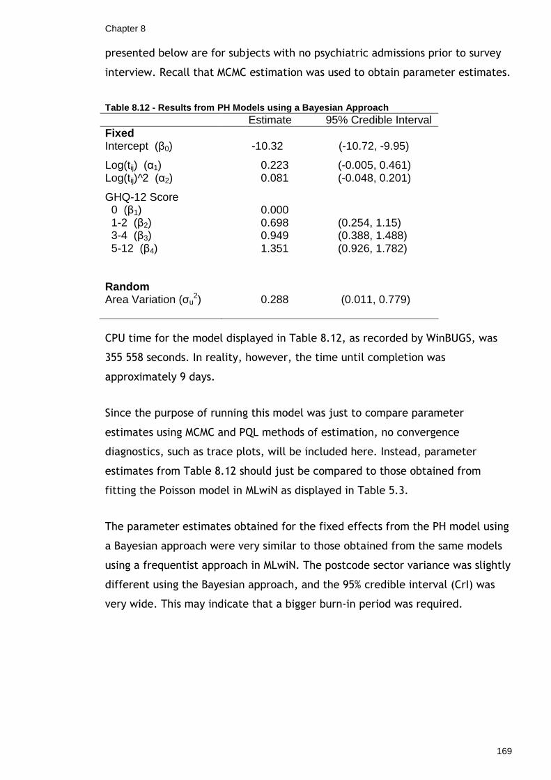
Chapter 8
169
presented below are for subjects with no psychiatric admissions prior to survey
interview. Recall that MCMC estimation was used to obtain parameter estimates.
Table 8.12 - Results from PH Models using a Bayesia n Approach Estimate 95% Credible Interval
Fixed Intercept (β0)
Log(tij) (α1) Log(tij)^2 (α2)
GHQ-12 Score 0 (β1) 1-2 (β2) 3-4 (β3) 5-12 (β4)
Random Area Variation (σu
2)
-10.32 (-10.72, -9.95)
0.223 (-0.005, 0.461) 0.081 (-0.048, 0.201)
0.000 0.698 (0.254, 1.15) 0.949 (0.388, 1.488) 1.351 (0.926, 1.782)
0.288 (0.011, 0.779)
CPU time for the model displayed in Table 8.12, as recorded by WinBUGS, was
355 558 seconds. In reality, however, the time until completion was
approximately 9 days.
Since the purpose of running this model was just to compare parameter
estimates using MCMC and PQL methods of estimation, no convergence
diagnostics, such as trace plots, will be included here. Instead, parameter
estimates from Table 8.12 should just be compared to those obtained from
fitting the Poisson model in MLwiN as displayed in Table 5.3.
The parameter estimates obtained for the fixed effects from the PH model using
a Bayesian approach were very similar to those obtained from the same models
using a frequentist approach in MLwiN. The postcode sector variance was slightly
different using the Bayesian approach, and the 95% credible interval (CrI) was
very wide. This may indicate that a bigger burn-in period was required.

Chapter 8
170
8.3.1.2 Summary of Bayesian Proportional Hazards Mo del Results
Section 8.3.1 discussed the application of Bayesian methods to survival
modelling, and why these methods may be more attractive than taking a
frequentist approach. Subsequent sections in this chapter will proceed to fit
frailty models using a Bayesian approach; however, it was firstly necessary to
demonstrate that MCMC estimation would produce similar estimates to those
obtained using PQL estimation. This ensures that Bayesian methods for fitting
multilevel survival models in WinBUGS are comparable to frequentist methods
employed to fit these models in MLwiN.
Comparison of MCMC and PQL estimation was carried out by fitting the same
continuous-time proportional hazards model using a Bayesian approach in
WinBUGS as was fitted previously in MLwiN (Section 5.4). The PH model took a
considerably longer time to run in WinBUGS using MCMC estimation than in
MLwiN using PQL estimation; however, as parameter estimates using the two
approaches (Bayesian and frequentist) were similar, this ensured that estimates
obtained using these different methods of estimation were comparable.
Confirmation of this now means that a new type of model may be tested as an
alternative to fitting continuous-time proportional hazard models in MLwiN – the
frailty model using a Bayesian approach. Results from these models are
presented in Section 8.3.2.
8.3.2 Fitting Frailty Models in WinBUGS
This section will present results obtained from fitting the shared frailty model in
WinBUGS. As discussed in Section 7.4.4.1, a Weibull distribution is assumed for
the survivor function with shape parameter, r, and scale parameter, µij. While
the Poisson model fitted in MLwiN required the dataset to be expanded into a
person-period dataset, thus leading to a vast increase in the size of the dataset,
no such expansion is required to fit frailty models in WinBUGS.
Since Section 8.3.1 of this chapter confirmed that PQL and MCMC estimation
were obtaining similar parameter estimates, results from the shared frailty

Chapter 8
171
model can be compared with results from the original Poisson model in Table
5.3. The Poisson model produced estimates of hazard ratios; therefore, in order
to be able to compare parameter estimates from the Poisson model and the
Weibull model fitted in WinBUGS, it was important to check that the parameter
estimates from the Weibull model fitted in WinBUGS could also be interpreted as
hazard ratios. Recall from 7.4.4 that the hazard function from fitting the
additive frailty model in WinBUGS is given as
h(tijxij, uj) = µijrtijr-1,
where
log(µij) = α + βTxij + uj.
Consider the baseline hazard for which all values of the covariates are zero, and
therefore the model contains an intercept, α, (and possibly random effects)
only. Consider also the hazard of event for an individual with covariate vector x.
Then, in the proportional hazards model, exp(βTx) represents the hazard ratio,
i.e. the hazard of event at time t for an individual with covariate vector x
relative to the baseline hazard. If the ratio of these hazards equals exp(βTx),
then the regression parameters from the additive frailty model fitted in
WinBUGS may be interpreted as hazard ratios.
( )( )
( )[ ]( )[ ] 1
1
0 exp
exp,−
−
+++
=rijj
rijjij
T
j
jijij
rtu
rtux
uth
uxth
αβα
=exp(BTxij) .
Therefore, the regression parameter estimates obtained from fitting the additive
frailty model in WinBUGS may be interpreted as hazard ratios.

Chapter 8
172
8.3.2.1 Results from Bayesian Frailty Models
This section presents results obtained from fitting a Weibull model to the
Scottish Health Survey data in WinBUGS. As before, the response was time until
first psychiatric admission as measured in days from Scottish Health Survey
interview, with any individuals who did not experience the event or who died
during follow-up being censored. Recall also that the primary interest was to
investigate the effect of GHQ-12 score on the hazard of first psychiatric
admission. Information was also available on a range of demographic,
socioeconomic and lifestyle risk factors.
Table 8.13 below displays results from fitting two Weibull models - one
containing GHQ-12 score only, and the other containing GHQ-12 score plus other
risk factors which were found to be significant when fitting the continuous-time
model in Section 5.4, referred to here as the ‘full model’. In other words, results
from Table 8.13 below should be compared to models B1 and B3 in Table 5.3.
Recall from Section 7.4.4.2 that the random effects (frailties) were given a log-
Normal prior, thus making the model a log-Normal frailty model. The random
effects standard deviation was given a Uniform prior, the shape parameter a log-
Normal prior, and finally, regression coefficients were given Normal priors.
Initial values were chosen based on parameter estimates obtained from fitting
the continuous-time Poisson model. For the model containing GHQ-12 score only,
a burn-in of 5000 iterations seemed to adequately achieve convergence, with a
further 41000 iterations after convergence to obtain posterior estimates. In the
model containing GHQ-12 score and all other significant risk factors, 25000
iterations were required for burn-in, with a further 50000 iterations on attaining
convergence. Convergence was assessed using trace plots (Figures 8.1 and 8.2)
and Gelman-Rubin plots (Figures 8.3 and 8.4). Note that, for the model
containing all significant covariates i.e. the full model, Figures 8.2 and 8.4 only
display trace plots and Gelman-Rubin plots for the intercept, GHQ-12 regression
parameters, shape and random effects variance. Trace plots and Gelman-Rubin
plots for all other significant covariates can be found in Appendix 3.

Chapter 8
173
Table 8.13 - Results from Weibull model GHQ-12 Only Full Model Estimate Credible Interval Estimate Credible Interval Fixed
Intercept (α) -12.2 (-13.26, -11.27) -12.87 (-14.36, -11.78)
GHQ-12 Score 0 0.000 0.000 1-2 (β1) 0.706 (0.27, 1.14) 0.475 (0.001, 0.92) 3-4 (β2) 0.956 (0.37, 1.48) 0.511 (-0.10, 1.09) 5-12 (β3) 1.368 (0.97, 1.78) 0.725 (0.26, 1.18)
Sex Male 0.000 Female (β4) -0.123 (-0.50, 0.25)
Age 16-24 0.000 25-34 (β5) -0.285 (-0.82, 0.29) 35-44 (β6) 0.024 (-0.51, 0.58) 45-54 (β7) -0.717 (-1.46, -0.02) 55-64 (β8) -0.321 (-0.97, 0.28) 65-74 (β9) 0.269 (-0.46, 0.99)
Marital Status Married/cohabiting 0.000 Other (β10) 0.351 (-0.01, 0.72)
Receipts of Benefits No 0.000 Yes (β11) 0.639 (0.22, 1.05)
Smoking Status Non-Smoker 0.000 Current Smoker (β12) 0.728 (0.32, 1.21) Ex-Smoker (β13) -0.032 (-0.69, 0.60)
Employment Status Full-Time 0.000 Unemployed (β14) 0.504 (-0.05, 1.04) Part-Time (β15) -0.339 (-0.82, 0.14)
Self-Assessed Health Very Good 0.000 Good (β16) 0.446 (-0.002, 0.90) Fair (β17) 0.897 (0.43, 1.38) Bad (β18) 0.001 (-1.24, 1.03) Very Bad (β19) 1.783 (0.81, 2.67)
Shape (r) 0.870 (0.74, 0.98) 0.866 (0.76, 1.04)
Random
Area Variation(σu2) 0.263 (0.001, 0.807) 0.307 (0.001, 0.91)

Chapter 8
174
alpha chains 1:2
iteration
5001 20000 40000
-14.0
-13.0
-12.0
-11.0
-10.0
beta[2] chains 1:2
iteration
5001 20000 40000
-0.5
0.0
0.5
1.0 1.5
2.0
beta[3] chains 1:2
iteration
5001 20000 40000
-1.0
0.0
1.0
2.0
beta[4] chains 1:2
iteration
5001 20000 40000
0.5
1.0
1.5
2.0
2.5
r chains 1:2
iteration
5001 20000 40000
0.7
0.8
0.9
1.0
1.1
sigma2.u2 chains 1:2
iteration
5001 20000 40000
0.0
0.5
1.0
1.5
Figure 8.1 - Trace plots for GHQ-12 only model

Chapter 8
175
alpha chains 1:2
iteration
25001 40000 60000
-15.0
-14.0
-13.0
-12.0
-11.0
beta[1] chains 1:2
iteration
25001 40000 60000
-0.5
0.0
0.5
1.0
1.5
beta[2] chains 1:2
iteration
25001 40000 60000
-1.0
0.0
1.0
2.0
beta[3] chains 1:2
iteration
25001 40000 60000
-0.5
0.0
0.5
1.0
1.5
r chains 1:2
iteration
25001 40000 60000
0.7
0.8
0.9
1.0
1.1
sigma2.u2 chains 1:2
iteration
25001 40000 60000
0.0
0.5
1.0
1.5
2.0
Figure 8.2 - Trace plots for full model
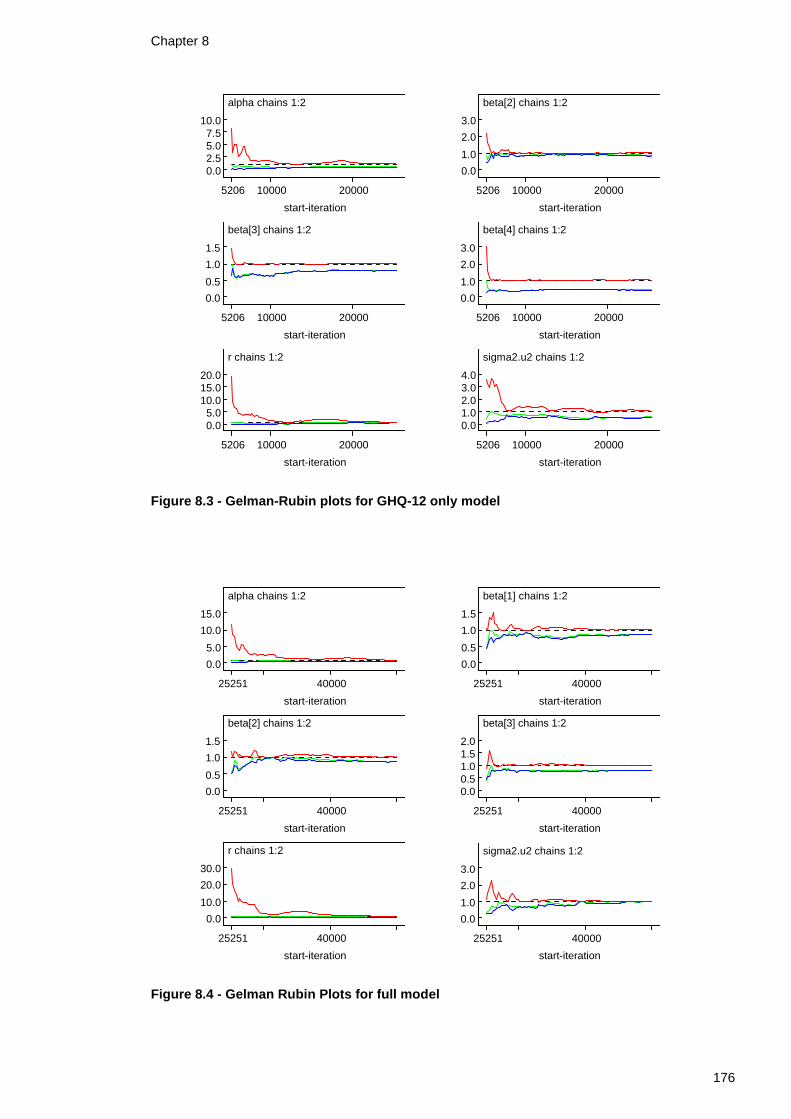
Chapter 8
176
alpha chains 1:2
start-iteration
5206 10000 20000
0.0 2.5 5.0 7.5 10.0
beta[2] chains 1:2
start-iteration
5206 10000 20000
0.0
1.0
2.0
3.0
beta[3] chains 1:2
start-iteration
5206 10000 20000
0.0
0.5
1.0
1.5
beta[4] chains 1:2
start-iteration
5206 10000 20000
0.0
1.0
2.0
3.0
r chains 1:2
start-iteration
5206 10000 20000
0.0 5.0 10.0 15.0 20.0
sigma2.u2 chains 1:2
start-iteration
5206 10000 20000
0.0 1.0 2.0 3.0 4.0
Figure 8.3 - Gelman-Rubin plots for GHQ-12 only mod el
alpha chains 1:2
start-iteration
25251 40000
0.0
5.0
10.0
15.0
beta[1] chains 1:2
start-iteration
25251 40000
0.0
0.5
1.0
1.5
beta[2] chains 1:2
start-iteration
25251 40000
0.0
0.5
1.0
1.5
beta[3] chains 1:2
start-iteration
25251 40000
0.0 0.5 1.0 1.5 2.0
r chains 1:2
start-iteration
25251 40000
0.0
10.0
20.0
30.0
sigma2.u2 chains 1:2
start-iteration
25251 40000
0.0
1.0
2.0
3.0
Figure 8.4 - Gelman Rubin Plots for full model
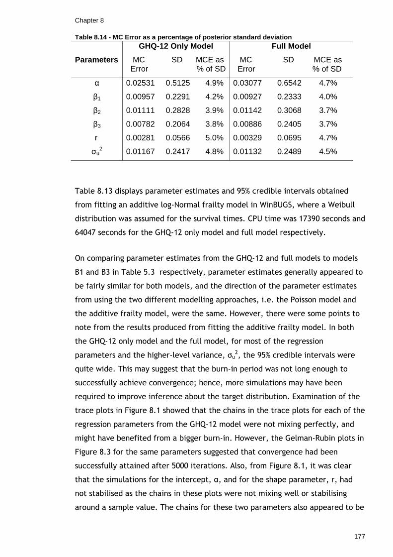
Chapter 8
177
Table 8.14 - MC Error as a percentage of posterior standard deviation
Parameters
GHQ-12 Only Model
MC SD MCE as Error % of SD
Full Model
MC SD MCE as Error % of SD
α
β1
β2
β3
r
σu2
0.02531 0.5125 4.9%
0.00957 0.2291 4.2%
0.01111 0.2828 3.9%
0.00782 0.2064 3.8%
0.00281 0.0566 5.0%
0.01167 0.2417 4.8%
0.03077 0.6542 4.7%
0.00927 0.2333 4.0%
0.01142 0.3068 3.7%
0.00886 0.2405 3.7%
0.00329 0.0695 4.7%
0.01132 0.2489 4.5%
Table 8.13 displays parameter estimates and 95% credible intervals obtained
from fitting an additive log-Normal frailty model in WinBUGS, where a Weibull
distribution was assumed for the survival times. CPU time was 17390 seconds and
64047 seconds for the GHQ-12 only model and full model respectively.
On comparing parameter estimates from the GHQ-12 and full models to models
B1 and B3 in Table 5.3 respectively, parameter estimates generally appeared to
be fairly similar for both models, and the direction of the parameter estimates
from using the two different modelling approaches, i.e. the Poisson model and
the additive frailty model, were the same. However, there were some points to
note from the results produced from fitting the additive frailty model. In both
the GHQ-12 only model and the full model, for most of the regression
parameters and the higher-level variance, σu2, the 95% credible intervals were
quite wide. This may suggest that the burn-in period was not long enough to
successfully achieve convergence; hence, more simulations may have been
required to improve inference about the target distribution. Examination of the
trace plots in Figure 8.1 showed that the chains in the trace plots for each of the
regression parameters from the GHQ-12 model were not mixing perfectly, and
might have benefited from a bigger burn-in. However, the Gelman-Rubin plots in
Figure 8.3 for the same parameters suggested that convergence had been
successfully attained after 5000 iterations. Also, from Figure 8.1, it was clear
that the simulations for the intercept, α, and for the shape parameter, r, had
not stabilised as the chains in these plots were not mixing well or stabilising
around a sample value. The chains for these two parameters also appeared to be

Chapter 8
178
correlated with each other. Finally, from Figure 8.1 it was observed that the
Gibbs sampler for the random effects variance was getting stuck near zero. Once
trapped here, the simulation may take a long time to escape [258]. A parameter
expansion scheme may be adopted to overcome slow convergence. This will be
considered in Section 8.3.5. Similar patterns for the full model were observed in
Figures 8.2 and 8.4.
Another way of assessing the accuracy of the posterior estimates is by comparing
the Monte Carlo error (MC error) and the sample standard deviation, as was
discussed in Section 7.4.6.3. A rule of thumb is that the MC error should be less
than around 5% of the sample standard deviation. For the GHQ-12 only model,
Table 8.14 shows that this was the case for all parameters. However, for most
parameters, the MC error was only just less than 5% of the sample standard
deviation, suggesting that more iterations may have been required after
achieving convergence. The same was true of the full model.
The shape parameter in the GHQ-12 only model in Table 8.13 was less than 1 (=
0.870) with 95% credible interval wholly less than 1. This suggested that the
hazard rate of event, when adjusting for GHQ-12 score, was strictly decreasing
in a nonlinear pattern as time increases. When the model was adjusted for all
further significant covariates, the shape parameter was still less than 1 (=
0.866); however, the 95% credible interval overlapped 1, indicating that it was
plausible that the hazard rate remained constant as time increased.
Several areas for consideration arose from fitting the additive frailty model to
the SHeS dataset. Firstly, the chains for the shape parameter and intercept
displayed in the trace plots in Figures 8.1 and 8.2 were very highly correlated.
Secondly, the Gibbs sampler was prone to getting trapped near zero for the
higher-level variance. As few individuals experienced the event of interest,
there were a large number of censored observations (approximately 99%). One
notion was that the problems were a consequence of the high percentage of
censoring, with the Weibull model perhaps not providing a ‘good fit’ in the
presence of many censored observations. To investigate this further a simulation
study was carried out. Full details are given in Section 8.3.3.
Chapter 8
179
8.3.3 Fitting Bayesian Frailty Models to a Simulate d Dataset
In the previous section it was discussed that the high percentage of censoring in
the SHeS dataset could be problematic when trying to fit the Weibull model. To
investigate this notion, a simulation study was carried out by simulating two
datasets – one which contained no censored observations and another which
contained a percentage of censored observations similar to that of the SHeS
dataset. Fitting models to both of these simulated datasets and comparing
results would indicate whether or not the high percentage of censoring was
posing a difficulty when trying to fit the Weibull model.
The simulated datasets had to be similar to the SHeS dataset in terms of size.
Recall that in the SHeS dataset there were 15305 individuals (with no psychiatric
admission prior to survey interview) nested within 624 postcode sectors;
therefore, the simulated datasets were specified to contain 15000 level-1 units
within 600 level-2 units. Recall also that the SHeS dataset was created from
information obtained from two different survey years, namely 1995 and 1998. It
is clear that those surveyed in 1995 would have a follow-up time of around 9
years, whereas those surveyed in 1998 would have a shorter-follow up time of 6
years (follow-up time was until 2004). The differences in follow-up times also
had to be accounted for when generating the simulated datasets. Parameter
estimates obtained from fitting the continuous-time Poisson model to the SHeS
data (Table 5.3) were used calculate the scale parameter, µ. This was required
when simulating the Weibull survival times, t, which were calculated using the
distribution’s inverse probability function [259] such that
( )[ ]rrndr
t1
ln−×= µ ,
where ‘rnd’ corresponded to the random numbers generated from the Uniform
distribution on the interval (0,1). The simulated datasets were created in MLwiN
and were then transferred into WinBUGS to fit the Weibull model.
The first point to investigate was the correlation in the chains for the intercept,
α, and the shape parameter, r. It was of interest to observe whether or not the
percentage of censored observations would have an effect on how these

Chapter 8
180
parameters behaved. Two models were fitted to both the simulated dataset with
no censoring and the simulated dataset with a percentage of censoring similar to
that of the actual SHeS dataset. The first model contained an intercept only (i.e.
no covariates or random effects) and fixed the shape parameter at 0.9 in the
Weibull distribution for survival times (recall from Table 8.13 that 0.9 was the
parameter estimate obtained for the shape parameter, r, when fitting the
Weibull model to the SHeS dataset); the second model was similar except that r
was not fixed and was specified to follow a log-Normal distribution. Parameter
estimates and 95% credible intervals are displayed in Table 8.15. Trace plots and
Gelman-Rubin plots are displayed in Figures 8.5 and 8.6.
Table 8.15 - Comparing intercept-only models betwee n all-event and highly censored simulated datasets r fixed at 0.9 r not fixed
Estimate 95% CrI Estimate 95% CrI No Censoring Intercept (α) Shape (r)
-10.0 (-10.02, -9.99) -9.999 (-10.12, -9.88) - - 0.900 (0.89, 0.91)
95% Censoring Intercept (α) Shape (r)
-10.06 (-10.13, -9.99) -10.48 (-11.08, -10.13) - - 0.953 (0.91, 1.03)
Figure 8.5 - Trace plots for intercept-only models from all-event & highly censored simulated datasets

Chapter 8
181
alpha chains 1:2
start-iteration
5061 8000 10000
0.0
0.5
1.0
alpha chains 1:2
start-iteration
5061 8000 10000
0.0 0.5 1.0 1.5 2.0
alpha chains 1:2
start-iteration
5061 8000 10000
0.0 0.5 1.0 1.5 2.0
alpha chains 1:2
start-iteration
5061 8000 10000
0.0
5.0
10.0
15.0
r chains 1:2
start-iteration
5061 8000 10000
0.0 0.5 1.0 1.5 2.0
r chains 1:2
start-iteration
5061 8000 10000
0.0 5.0 10.0 15.0 20.0
No censoring, r fixed Censoring, r fixed
No censoring, r not fixed
No censoring, r not fixed
Censoring, r not fixed
Censoring, r not fixed
Figure 8.6 - Gelman-Rubin plots for intercept-only models from uncensored & highly censored simulated datasets
As in the frailty model fitted in Section 8.3.2.1, the intercept, α, was given a
Normal(0, 0.0001) prior, and the shape parameter, r, a log-Normal(0, 0.1) prior.
For each of the four models in Table 8.15 above, a burn-in period of 5000
iterations was used before running a further 12000 iterations to obtain the
parameter estimates displayed. The average CPU time for the four models was
2644 seconds.
When comparing results from fitting the four models displayed in Table 8.15,
generally there was not much of a difference in the parameter estimates for
alpha and r respectively. However, there were some points to note. It was
mentioned previously that parameter estimates obtained from fitting the Poisson
model to the SHeS data (Table 5.3) were used in the simulation, i.e. a value of

Chapter 8
182
-10 for alpha. The value of 0.9 for r was obtained from fitting the Weibull model
to the SHeS data (Table 8.13). When examining the results in Table 8.15, the
parameter estimates for alpha and r (where applicable) were all close to these
respective values; however, when looking at results from the model containing
both alpha and r which was fitted to the simulated dataset with a high
percentage of censoring, the 95% credible interval for alpha did not include -10
and, similarly, the 95% credible interval for r did not include 0.9. The trace plots
in Figure 8.5 were used to determine how well the parameters are behaving. For
the model containing alpha only fitted to the simulated dataset with no
censoring, the trace plot indicated that the multiple chains were mixing well,
and hence convergence looked reasonable. The parameter estimate of alpha
from this model was exactly -10, with a very narrow 95% CrI. When the same
model (intercept only) was fitted to the simulated dataset containing the high
percentage of censoring, the multiple chains in the trace plot were not mixing
quite as well as when there were no censored observations; however,
convergence still looked reasonable, and the Gelman-Rubin plot in Figure 8.6
also indicated that a burn-in period of 5000 seemed sufficient enough to achieve
convergence. The 95% CrI, however, was slightly wider when censoring was
present than when the same model was fitted to the simulated dataset
containing no censoring.
When the shape parameter was no longer fixed at 0.9 in the Weibull distribution,
the multiple chains in the trace plot for the model (now containing both alpha
and r) fitted to the simulated dataset with no censoring were not mixing very
well for either parameter, with evidence of correlation between the chains for
the two parameters. The Gelman-Rubin plots in Figure 8.6 indicated that a
bigger burn-in period may have been required (perhaps around 9000 iterations).
When comparing the two models fitted to the simulated dataset containing no
censored observations, the 95% credible interval for the intercept in the model
when r was not fixed was wider than that obtained when r was fixed at 0.9;
however, -10 was still included in the range of plausible values. Finally, the
multiple chains in trace plots for the model fitted to the highly censored
simulated dataset when r was not fixed at 0.9 were not mixing at all for either
parameter and again there appeared to be correlation between the chains for
the two parameters. Neither of the 95% credible intervals for alpha and r

Chapter 8
183
overlapped the respective values of -10 or 0.9, which were the values expected
for those parameters.
Up to this point, the simulation study showed that having a high percentage of
censored observations had a slight effect on the results. Parameter estimates
were the least precise when censoring was present, as opposed to when there
were no censored observations; however, there was still correlation between the
chains for the intercept and the shape parameter when there were no censored
observations, although the multiple chains were mixing better. It is of interest
to reduce the correlation in the Markov chains in order to reduce the number of
iterations required, thus speeding up computing time. Ways of eliminating this
correlation are considered in Section 8.3.4.
8.3.4 Reducing Correlation in the Weibull Model
Consider a Weibull distribution with shape parameter r and scale parameter µ. In
WinBUGS notation this is X ~ dweib(r, µ) and the probability density function,
p(x), is given as
p(x) = r µxr-1exp(-µxr); x>0 .
The expectation of X is thus given as
E(X) = µ -1/rΓ(1 + 1/r) .
The value of E(X) will be pinned down by the data and
µ -1/rΓ(1 + 1/r) ≈ constant, k say .
Taking the natural logarithm, this becomes
-1/r log(µ) + log[Γ(1 + 1/r)] ≈ k
i.e. log(µ) ≈ -rk - log[Γ(1 + 1/r)
Equation 8.1

Chapter 8
184
Suppose, for the purpose of illustration, that the model to be fitted contains an
intercept, α, only, i.e. there are no covariates or random effects. Then log(µ) =
α. Thus, from Equation 8.1, it is clear that the posterior negative correlation
observed between α and r is not surprising (especially if r is close to 1).
Consider, instead, the probability density function for an alternative
parameterisation of the Weibull distribution,
p(x) = r/λ(x/λ)r-1exp[-(x/λ)r]; x>0 ,
= (r/ λr)xr-1exp[-(xr/λr)] ,
for a Weibull distribution with shape parameter r and scale parameter λ. Now
the expected value of X is given as
E(X) = λΓ(1 + 1/r) .
This re-parameterisation should lead to a posterior for (r, λ) with less
correlation. It is clear from the re-parameterisation that
µ = 1/λr .
Thus, for a model containing an intercept only the model is written in WinBUGS
as

Chapter 8
185
This may be extended to include covariates and random effects. The form of the
model including all significant covariates and random effects, as written in
WinBUGS, can be found in Appendix 4.
Using the re-parameterised version of the scale parameter, µ, a model
containing only an intercept, i.e. log(µ) = α, was fitted to both simulated
datasets, i.e. with no censored observations and with a high percentage of
censored observations. This was done in order to investigate if the correlation
between alpha and the shape parameter had been reduced. GHQ-12 score was
then added to the model before adding all covariates to fit the full model in
order to see what effect adding further covariates to the model would have.
Results are displayed in Table 8.16 below. Trace plots for alpha, r and the
higher-level variance, σu2, as well as for the GHQ-12 score regression parameters
(where applicable) are displayed in Figures 8.7 and 8.8. Corresponding Gelman-
Rubin plots are displayed in Figures 8.9 and 8.10. Trace plots and Gelman-Rubin
plots for the other significant covariates in the full model are not displayed
here.

186
Table 8.16 - Results from re-parameterised model fi tted to simulated data No Censoring 80% Censoring
Intercept GHQ-12 Full Est. 95%CrI Est. 95%CrI Est. 95%CrI
Intercept GHQ-12 Full Est. 95%CrI Est. 95%CrI Est. 95%CrI
Fixed
Intercept (α)
GHQ-12 Score 0 1-2 (β1) 3-4 (β2) 5-12 (β3)
Sex Male Female (β4)
Age 16-24 25-34 (β5) 35-44 (β6) 45-54 (β7) 55-64 (β8) 65-74 (β9)
Marital Status Married/cohabiting Other (β10)
Receipts of Benefits No Yes (β11)
Smoking Status Non-Smoker Current Smoker (β12) Ex-Smoker (β13)
-10.0 (-10.14, -9.88) -9.9 (-10.09, -9.81) -10.9 (-11.09, -10.76)
0 0 0.68 (0.64, 0.72) 0.98 (0.93, 1.02) 0.86 (0.80, 0.92) 1.58 (1.51, 1.64) 1.27 (1.21, 1.32) 2.84 (2.77, 2.90) 0 -0.26 (-0.29, -0.23)
0 -0.42 (-0.48, -0.35) 0.20 (0.14, 0.26) -2.67 (-2.74, -2.60) -1.43 (-1.50, -1.37) 1.25 (1.17, 1.32)
0 0.76 (0.73, 0.80)
0 1.20 (1.16, 1.24)
0 0.70 (0.66, 0.74) 0.02 (-0.02, 0.06)
-10.5 (-11.1, -9.96) -10.5 (-10.85, -10.07) -11.0 (-11.31, -10.71)
0 0 0.61 (0.47, 0.74) 0.91 (0.80, 1.02) 0.78 (0.61, 0.95) 1.59 (1.46, 1.71) 1.23 (1.10, 1.36) 2.82 (2.72, 2.93) 0 -0.28 (-0.35, -0.20)
0 -0.50 (-0.62, -0.37) 0.15 (0.04, 0.27) -2.71 (-2.93, -2.50) -1.45 (-1.60, -1.28) 1.16 (1.02, 1.30)
0 0.71 (0.64, 0.79)
0 1.20 (1.12, 1.28)
0 0.63 (0.55, 0.72) 0.04 (-0.07, 0.14)

187
Employment Status Full-Time Unemployed (β14) Part-Time (β15)
Self-Assessed Health Very Good Good (β16) Fair (β17) Bad (β18) Very Bad (β19)
Shape (r)
Random
Area Variation(σu2)
0 0.53 (0.46, 0.61) -0.64 (-0.68, -0.60)
0 1.02 (0.98, 1.06) 2.86 (2.79, 2.92) 0.73 (0.61, 0.84) 8.67 (8.44, 8.90)
0.90 (0.89, 0.91) 0.90 (0.89, 0.91) 0.90 (0.88, 0.91)
0.24 (0.21, 0.27) 0.25 (0.22, 0.29)
0 0.40 (0.26, 0.55) -0.70 (-0.81, -0.59)
0 0.99 (0.90, 1.09) 2.86 (2.75, 2.96) 0.63 (0.34, 0.90) 8.82 (8.51, 9.11)
0.95 (0.89, 1.03) 0.96 (0.91, 1.01) 0.93 (0.90, 0.96)
0.33 (0.25, 0.43) 0.27 (0.21, 0.33)
alpha chains 1:2
iteration
5001 10000 15000
-10.4
-10.2
-10.0
-9.8
-9.6
r chains 1:2
iteration
5001 10000 15000
0.86
0.88
0.9
0.92
0.94
Intercept-only model
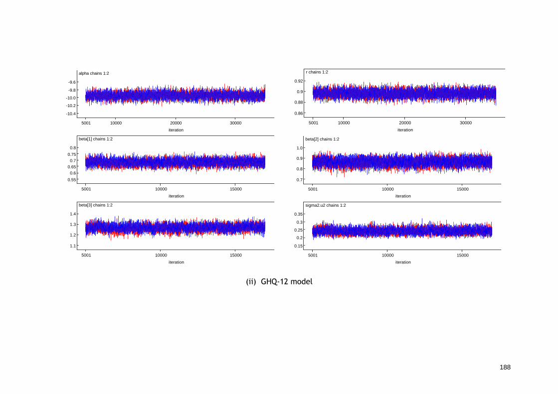
188
alpha chains 1:2
iteration
5001 10000 20000 30000
-10.4
-10.2
-10.0
-9.8
-9.6
r chains 1:2
iteration
5001 10000 20000 30000
0.86
0.88
0.9
0.92
beta[1] chains 1:2
iteration
5001 10000 15000
0.55
0.6
0.65
0.7
0.75
0.8
beta[2] chains 1:2
iteration
5001 10000 15000
0.7
0.8
0.9
1.0
beta[3] chains 1:2
iteration
5001 10000 15000
1.1
1.2
1.3
1.4
sigma2.u2 chains 1:2
iteration
5001 10000 15000
0.15
0.2
0.25
0.3
0.35
(ii) GHQ-12 model

189
alpha chains 1:2
iteration
10001 15000 20000 25000
-11.4
-11.2
-11.0 -10.8
-10.6
-10.4
r chains 1:2
iteration
10001 15000 20000 25000
0.86
0.88
0.9
0.92
0.94
beta[1] chains 1:2
iteration
10001 15000 20000 25000
0.85
0.9
0.95
1.0
1.05
1.1
beta[2] chains 1:2
iteration
10001 15000 20000 25000
1.4
1.5
1.6
1.7
1.8
beta[3] chains 1:2
iteration
10001 15000 20000 25000
2.6
2.7
2.8
2.9
3.0
sigma2.u2 chains 1:2
iteration
10001 15000 20000 25000
0.15
0.2
0.25
0.3
0.35
(iii) Full Model
Figure 8.7 - Trace plots for re-parameterised model fitted to simulated dataset with no censoring

190
alpha chains 1:2
iteration
5001 10000 20000 30000
-11.5
-11.0
-10.5
-10.0
-9.5
r chains 1:2
iteration
5001 10000 20000 30000
0.8
0.9
1.0
1.1
(i) Intercept only model

191
alpha chains 1:2
iteration
5001 10000 20000 30000
-11.5
-11.0
-10.5
-10.0
-9.5
r chains 1:2
iteration
5001 10000 20000 30000
0.8
0.85
0.9
0.95
1.0
1.05
beta[1] chains 1:2
iteration
5001 10000 20000 30000
0.2
0.4
0.6
0.8
1.0
beta[2] chains 1:2
iteration
5001 10000 20000 30000
0.4
0.6
0.8
1.0
1.2
beta[3] chains 1:2
iteration
5001 10000 20000 30000
0.8
1.0
1.2
1.4
1.6
sigma2.u2 chains 1:2
iteration
5001 10000 20000 30000
0.0
0.2
0.4
0.6
(ii) GHQ-12 model

192
alpha chains 1:2
iteration
10001 15000 20000 25000
-12.0
-11.5
-11.0
-10.5
r chains 1:2
iteration
10001 15000 20000 25000
0.85
0.9
0.95
1.0
beta[1] chains 1:2
iteration
10001 15000 20000 25000
0.6
0.8
1.0
1.2
beta[2] chains 1:2
iteration
10001 15000 20000 25000
1.2
1.4
1.6
1.8
2.0
beta[3] chains 1:2
iteration
10001 15000 20000 25000
2.6
2.8
3.0
3.2
sigma2.u2 chains 1:2
iteration
10001 15000 20000 25000
0.1
0.2
0.3
0.4
0.5
(iii) Full Model
Figure 8.8 - Trace plots for re-parameterised model fitted to simulated dataset with censoring
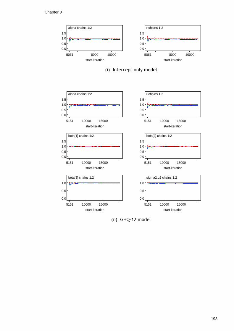
Chapter 8
193
alpha chains 1:2
start-iteration
5061 8000 10000
0.0
0.5
1.0
1.5
r chains 1:2
start-iteration
5061 8000 10000
0.0
0.5
1.0
1.5
(i) Intercept only model
alpha chains 1:2
start-iteration
5151 10000 15000
0.0
0.5
1.0
1.5
r chains 1:2
start-iteration
5151 10000 15000
0.0
0.5
1.0
1.5
beta[1] chains 1:2
start-iteration
5151 10000 15000
0.0
0.5
1.0
1.5
beta[2] chains 1:2
start-iteration
5151 10000 15000
0.0
0.5
1.0
1.5
beta[3] chains 1:2
start-iteration
5151 10000 15000
0.0
0.5
1.0
sigma2.u2 chains 1:2
start-iteration
5151 10000 15000
0.0
0.5
1.0
(ii) GHQ-12 model

Chapter 8
194
alpha chains 1:2
start-iteration
10076 12000 14000 16000
0.0
0.5
1.0
1.5
r chains 1:2
start-iteration
10076 12000 14000 16000
0.0
0.5
1.0
1.5
beta[1] chains 1:2
start-iteration
10076 12000 14000 16000
0.0
0.5
1.0
1.5
beta[2] chains 1:2
start-iteration
10076 12000 14000 16000
0.0
0.5
1.0
1.5
beta[3] chains 1:2
start-iteration
10076 12000 14000 16000
0.0
0.5
1.0
1.5
sigma2.u2 chains 1:2
start-iteration
10076 12000 14000 16000
0.0
0.5
1.0
1.5
(iii) Full model
Figure 8.9 - Gelman-Rubin plots for re-parameterise d model fitted to simulated dataset with no censoring
alpha chains 1:2
start-iteration
5151 10000 15000
0.0
1.0
2.0
3.0
r chains 1:2
start-iteration
5151 10000 15000
0.0
1.0
2.0
3.0
(i) Intercept only model

Chapter 8
195
alpha chains 1:2
start-iteration
5151 10000 15000
0.0
0.5
1.0
1.5
r chains 1:2
start-iteration
5151 10000 15000
0.0 0.5 1.0 1.5 2.0
beta[1] chains 1:2
start-iteration
5151 10000 15000
0.0
0.5
1.0
1.5
beta[2] chains 1:2
start-iteration
5151 10000 15000
0.0
0.5
1.0
1.5
beta[3] chains 1:2
start-iteration
5151 10000 15000
0.0
0.5
1.0
1.5
sigma2.u2 chains 1:2
start-iteration
5151 10000 15000
0.0
0.5
1.0
1.5
(ii) GHQ-12 model
alpha chains 1:2
start-iteration
10076 12000 14000 16000
0.0
0.5
1.0
1.5
r chains 1:2
start-iteration
10076 12000 14000 16000
0.0
0.5
1.0
1.5
beta[1] chains 1:2
start-iteration
10076 12000 14000 16000
0.0
0.5
1.0
1.5
beta[2] chains 1:2
start-iteration
10076 12000 14000 16000
0.0
0.5
1.0
1.5
beta[3] chains 1:2
start-iteration
10076 12000 14000 16000
0.0
0.5
1.0
1.5
sigma2.u2 chains 1:2
start-iteration
10076 12000 14000 16000
0.0
0.5
1.0
1.5
(iii) Full model
Figure 8.10 - Gelman-Rubin plots for re-parameteris ed model fitted to simulated dataset with censoring

Chapter 8
196
The trace plots in Figures 8.7 and 8.8 can be examined in order to investigate
whether re-parameterising the scale parameter, µ, in terms of λ has reduced the
correlation in the Markov chains between the intercept, α, and the shape
parameter, r. Recall that three models were fitted to both the simulated dataset
with no censored observations and the simulated dataset with a high percentage
of censored observations: a model including an intercept only; a model
including GHQ-12 score and random effects; and a full model including all
significant covariates (as determined when fitting the Poisson model displayed in
Table 5.3) and random effects.
The trace plots in Figure 8.7 were obtained from fitting the three models
described to the simulated dataset with no censored observations. Firstly, from
observing the trace plots for the model containing the intercept only (Figure 8.7
(i)), it was clear that the correlation between alpha and r had been reduced,
with the multiple chains for each of these parameters mixing well and having
stabilised around the respective sample values of -10 and 0.9. When comparing
this to the trace plots obtained from the same model fitted without the re-
parameterisation (Figure 8.5), it could be seen that the plots obtained from the
model with the re-parameterisation behaved much better than those without
and had achieved convergence after a burn-in period of 5000 iterations. This was
not the case for the plots from the model without the re-parameterisation. GHQ-
12 score and the random effects were then added to this model to see whether
or not including any covariates would affect results. All trace plots obtained
from fitting the model with the re-parameterisation behaved well. There was no
indication of any correlation between alpha and r, and a burn-in of 5000
iterations had been sufficient to achieve convergence. Finally, all other
significant covariates were added to the model including GHQ-12 score. Trace
plots for the significant covariates, other than GHQ-12 score, are not displayed
here; however, the multiple chains in the trace plots for all other parameters
were mixing well, and there was no evidence of any correlation between alpha
and r.
The trace plots in Figure 8.8 were those obtained from fitting the same three
models to the simulated dataset with a high percentage of censored
observations. Comparing the trace plots from the model including an intercept
only (Figure 8.8 (i)) to the trace plots in Figure 8.5 obtained from fitting the

Chapter 8
197
same model without the re-parameterisation, it could be seen that re-
parameterising greatly reduced the correlation between alpha and r. The
multiple chains for both parameters were mixing much better after a burn-in
period of 5000 iterations than they had been for the model without the re-
parameterisation after the same burn-in period. However, the high percentage
of censoring seemed to slightly affect results. When the trace plots from Figure
8.8 (i) were compared to those in 8.7 (i), the multiple chains in the plots in
Figure 8.8 (i) were not mixing quite as well. This suggested that a bigger burn-in
period may have been required (in the presence of censoring) in order to achieve
convergence. The Gelman-Rubin plots for alpha and r in Figure 8.10 (i) suggested
that a burn-in period of at least 12000 iterations may have been required to
achieve convergence. GHQ-12 score and the random effects were then added to
the re-parameterised model fitted to the simulated dataset with a high
percentage of censored observations. Examination of the trace plots obtained
from this model (displayed in Figure 8.8 (ii)) showed that the correlation
between alpha and r had been reduced further on addition of GHQ-12 score to
the model. The multiple chains for alpha and r were mixing much better than
they had been when the re-parameterised model including only an intercept had
been fitted to the same data. Comparing this re-parameterised model (Figure
8.8 (ii)) to the same model fitted to the simulated dataset with no censoring
(Figure 8.7 (ii)), suggested that the multiple chains for alpha and r were not
mixing quite as well after the same burn-in period (5000 iterations) in the
presence of censoring; however, the difference was minimal. Finally, all
significant covariates were added to the re-parameterised model fitted to the
simulated dataset with a high percentage of censored observations. The multiple
chains in the trace plots for alpha and r (Figure 8.8 (iii)) were mixing fairly well
following a burn-in period of 10000 iterations; however, there was perhaps the
suggestion from the Gelman-Rubin plots for this model, displayed in Figure 8.10
(iii), that a burn-in period of 13000 iterations may have been more sufficient for
achieving convergence. Censoring appeared to have had a small effect on the
results. When the trace plots from this model were compared to the trace plots
from the same model fitted to the simulated dataset with no censored
observations (Figure 8.7 (iii)); there was some evidence that the multiple chains
for alpha and r, in the presence of censoring, were not behaving as well as when

Chapter 8
198
there were no censored observations after the same burn-in period (10000
iterations).
Parameter estimates obtained from fitting the three models to both the
simulated dataset without censoring and the simulated dataset with a high
percentage of censoring are displayed in Table 8.16. Recall that the parameter
estimates used for creating the simulated dataset (i.e. in the calculation of the
scale parameter, µ) were those obtained from fitting the continuous-time
Poisson model to the SHeS data (Table 5.3); therefore, parameter estimates
when fitting the three (re-parameterised) Weibull models to the simulated
datasets should be similar to those in Table 5.3. On inspection of the results in
Table 8.16, it can be seen that, when the (re-parameterised) model containing
an intercept only and the model which also contained GHQ-12 score were fitted
to the simulated dataset without censoring, all parameter estimates were close
to the values used in the simulation. Additionally, all 95% credible intervals
overlapped the values used in the simulation for each parameter. Apart from the
intercept in the GHQ-12-only model, this was also the case when the intercept-
only model and model containing GHQ-12 score were fitted to the simulated
dataset with the high percentage of censoring. It should be noted that the 95%
credible intervals in the models fitted to the simulated dataset with a high
percentage of censored observations were wider than those from the models
fitted to the simulated dataset with no censoring. The parameter estimate for
intercept in the model with GHQ-12 score, however, was smaller than expected
(-10.5 as opposed to -10), and the 95% credible interval did not overlap -10.
When fitting the models with all significant covariates to both simulated
datasets (i.e. no censoring and a high percentage of censoring), parameter
estimates for most of the covariates were not close to those used when creating
the simulated dataset (i.e. obtained from model B3 in Table 5.3), and the 95%
credible intervals did not contain these respective values.
To summarise, it appears that re-parameterising the scale parameter in the
Weibull model reduced the correlation in the Markov chains between the
intercept, α, and the shape parameter, r. This meant that the burn-in period
required to achieve convergence using the re-parameterised model was shorter
than that required for the model without the re-parameterisation. Hence, the
re-parameterised model could be estimated in a shorter time. Fitting models to

Chapter 8
199
simulated datasets with both no censored observations and a high percentage of
censored observations revealed that a high percentage of censoring only had a
minimal effect on the results and computing time. Thus, it was of interest to go
on to fit the re-parameterised model to the actual SHeS dataset, a dataset
which contained a high percentage of censored observations, to discover
whether or not the re-parameterisation would work with the real dataset.
8.3.4.1 Fitting the Re-parameterised Model to the S cottish Dataset
This section displays results obtained from fitting the re-parameterised model to
the Scottish Health Survey dataset. Recall that the purpose of the re-
parameterised model was to reduce the correlation in the Markov chains
between the intercept parameter, α, and the shape parameter, r, in order to
reduce the number of iterations required, hence speeding up computing time.
Parameter estimates obtained from fitting a model containing GHQ-12 score
only, and a model containing all significant covariates, are presented in Table
8.17. The respective trace plots and Gelman-Rubin plots are given in Figures
8.11 and 8.12 and Figures 8.13 and 8.14. Note that only trace plots and Gelman-
Rubin plots for the intercept, GHQ-12 regression parameters, shape parameter
and higher level variance, σu2, are presented. Plots for all other covariates are
not included here.
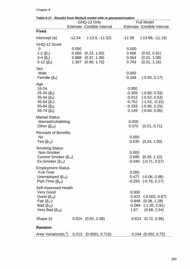
Chapter 8
200
Table 8.17 - Results from Weibull model with re-par ameterisation GHQ-12 Only Full Model Estimate Credible Interval Estimate Credible Interval Fixed
Intercept (α) -12.54 (-13.9, -11.52) -12.39 (-13.88, -11.19)
GHQ-12 Score 0 0.000 0.000 1-2 (β1) 0.656 (0.23, 1.05) 0.466 (0.02, 0.91) 3-4 (β2) 0.888 (0.37, 1.38) 0.554 (0.01, 1.08) 5-12 (β3) 1.307 (0.90, 1.72) 0.743 (0.31, 1.16)
Sex Male 0.000 Female (β4) -0.184 (-0.50, 0.17)
Age 16-24 0.000 25-34 (β5) -0.309 (-0.80, 0.33) 35-44 (β6) -0.013 (-0.52, 0.53) 45-54 (β7) -0.752 (-1.52, -0.15) 55-64 (β8) -0.333 (-0.90, 0.25) 65-74 (β9) 0.149 (-0.64, 0.85)
Marital Status Married/cohabiting 0.000 Other (β10) 0.370 (0.01, 0.71)
Receipts of Benefits No 0.000 Yes (β11) 0.635 (0.24, 1.00)
Smoking Status Non-Smoker 0.000 Current Smoker (β12) 0.695 (0.29, 1.10) Ex-Smoker (β13) -0.040 (-0.71, 0.57)
Employment Status Full-Time 0.000 Unemployed (β14) 0.477 (-0.06, 0.98) Part-Time (β15) -0.293 (-0.76, 0.17)
Self-Assessed Health Very Good 0.000 Good (β16) 0.422 (-0.002, 0.87) Fair (β17) 0.848 (0.38, 1.28) Bad (β18) -0.084 (-1.35, 0.91) Very Bad (β19) 1.67 (0.68, 2.54) Shape (r) 0.924 (0.81, 0.98) 0.823 (0.72, 0.96) Random
Area Variation(σu2) 0.213 (0.0001, 0.716) 0.244 (0.002, 0.75)

201
alpha chains 1:2
iteration
25001 40000 60000
-15.0
-14.0
-13.0
-12.0
-11.0
-10.0
r chains 1:2
iteration
25001 40000 60000
0.7
0.8
0.9
1.0
1.1
1.2
beta[2] chains 1:2
iteration
25001 40000 60000
-0.5
0.0
0.5
1.0
1.5
beta[3] chains 1:2
iteration
25001 40000 60000
-1.0
0.0
1.0
2.0
beta[4] chains 1:2
iteration
25001 40000 60000
0.0
0.5
1.0
1.5
2.0
2.5
sigma2.u2 chains 1:2
iteration
25001 40000 60000
0.0
0.5
1.0
1.5
Figure 8.11 - Trace plots for re-parameterised GHQ- 12 model

202
alpha chains 1:2
iteration
25001 40000 60000
-16.0
-14.0
-12.0
-10.0
r chains 1:2
iteration
25001 40000 60000
0.6
0.7
0.8
0.9
1.0
1.1
beta[1] chains 1:2
iteration
25001 40000 60000
-0.5
0.0
0.5
1.0
1.5
beta[2] chains 1:2
iteration
25001 40000 60000
-1.0
-0.5
0.0
0.5
1.0
1.5
beta[3] chains 1:2
iteration
25001 40000 60000
0.0
0.5
1.0
1.5
sigma2.u2 chains 1:2
iteration
25001 40000 60000
0.0
0.25
0.5
0.75
1.0
Figure 8.12 - Trace plots for re-parameterised full model

Chapter 8
203
alpha chains 1:2
start-iteration
25251 40000
0.0 0.5 1.0 1.5 2.0
r chains 1:2
start-iteration
25251 40000
0.0
1.0
2.0
3.0
beta[2] chains 1:2
start-iteration
25251 40000
0.0 0.5 1.0 1.5 2.0
beta[3] chains 1:2
start-iteration
25251 40000
0.0 0.5 1.0 1.5 2.0
beta[4] chains 1:2
start-iteration
25251 40000
0.0
1.0
2.0
3.0
sigma2.u2 chains 1:2
start-iteration
25251 40000
0.0
1.0
2.0
3.0
Figure 8.13 - Gelman-Rubin plots for re-parameteris ed GHQ-12 model
alpha chains 1:2
start-iteration
25251 40000
0.0
1.0
2.0
3.0
r chains 1:2
start-iteration
25251 40000
0.0
2.0
4.0
beta[1] chains 1:2
start-iteration
25251 40000
0.0 1.0 2.0 3.0 4.0
beta[2] chains 1:2
start-iteration
25251 40000
0.0
1.0
2.0
3.0
beta[3] chains 1:2
start-iteration
25251 40000
0.0 1.0 2.0 3.0 4.0
sigma2.u2 chains 1:2
start-iteration
25251 40000
0.0
1.0
2.0
3.0
Figure 8.14 - Gelman-Rubin plots for re-parameteris ed full model

Chapter 8
204
Parameter estimates displayed in Table 8.17 for both the GHQ-12 model and the
full model were obtained from running 50000 iterations following a burn-in
period of 25000 iterations. From examination of the trace plots in Figures 8.11
and 8.12, and comparing them to the trace plots in Figures 8.7 and 8.8, it can be
seen that the re-parameterisation did not perform as well when fitting the
model to the real SHeS dataset as it did with the simulated datasets. There still
appeared to be correlation in the multiple chains for the intercept and shape
parameter even when using the re-parameterised model. Although the multiple
chains did appear to be mixing better than they had been without the re-
parameterisation (Figures 8.1 and 8.3), this may just have been a result of
running more iterations. However, for the full model with and without the re-
parameterisation, the burn-in period and the number of iterations after burn-in
were the same. The trace plots for the intercept and shape parameter were
mixing better in Figure 8.12 than in Figure 8.2; this would support the use of the
re-parameterised model. Trace plots for the GHQ-12 regression parameters in
Figures 8.11 and 8.12 behaved fairly well, with sufficient mixing of the multiple
chains for each; however, the Gelman-Rubin plots for these parameters,
displayed in Figures 8.13 and 8.14, suggested that a burn-in period of 35000
iterations may have been more sufficient for achieving convergence. Finally,
from observing the trace plot for the higher-level variance, σu2, it can be seen
that the Gibbs sampler was still getting trapped near zero, leading to slow
convergence for this parameter. This may be overcome using a parameter
expansion scheme which is investigated further in Section 8.3.5.
The parameter estimates obtained from fitting the re-parameterised model to
the SHeS dataset (Table 8.17) were compared to those obtained from fitting the
model without the re-parameterisation (Table 8.13). Parameter estimates and
95% credible intervals for both the GHQ-12 model and the full model using the
re-parameterisation were very similar to those from the original Weibull model.
Still perhaps of concern, however, was the 95% credible interval for the higher-
level variance, σu2. Intervals for this parameter in both the GHQ-12 model and
the full model were very wide; however, successful implementation of the
parameter expansion scheme could possibly lead to more precise interval
estimates.

Chapter 8
205
8.3.5 Parameter Expansion in the Weibull Model
Trace plots for the higher-level variance in Figures 8.11 and 8.12 indicated that
the Gibbs sampler was getting trapped near zero, hence leading to slow
convergence for this parameter. Parameter expansion can be effective when the
variance parameter in random-effects models gets trapped near zero. The
technique was originally developed to speed up the EM algorithm by Liu et al.
[260]; however, it has since also been considered in relation to MCMC sampling
and the Gibbs sampler [261]. The parameter expansion technique works by
embedding the model of interest in a larger model by including additional
redundant parameters. The larger parameter is unidentified; however, the
embedded model is still identifiable, and parameters may be extracted [207].
The aim of the parameter expansion technique is to try to reduce the correlation
between the random-effects chains and the chain for their variance by
introducing an additional parameter that updates the random effects and their
variance simultaneously [207]. Each set of residuals is multiplied by an
additional parameter, a, say. The parameter expansion technique was adopted
for the re-parameterised Weibull model. For a model containing GHQ-12 score
only, the re-parameterised Weibull model with parameter expansion was written
in WinBUGS as follows:

Chapter 8
206
The original parameters are thus given by
uj = avj , σu2 = a2σv
2 ,
as indicated in lines 6 and 33 of the above WinBUGS code, respectively. Browne
[262] discussed that as the ‘a’ parameters multiply both the variance and the
residuals, the sampler is given a quick route out of the part of the posterior near
the origin. Parameter estimates obtained from fitting this model are displayed in
Table 8.18. Trace plots and Gelman-Rubin plots are given in Figures 8.15 – 8.18.
As well as GHQ-12 score only, the model was also extended to include all
significant covariates, i.e. the full model. Note that, as in previous sections,
trace plots and Gelman-Rubin plots are only displayed for the intercept, shape
parameter, higher-level variance and the GHQ-12 regression parameters. Plots
for the other covariates are not included.

Chapter 8
207
Table 8.18 - Results of re-parameterised Weibull mo del with variance expansion GHQ-12 Only Full Model Estimate 95% CrI Estimate 95% CrI Fixed
Intercept (α) -12.47 (-1367, -11.44) -12.16 (-13.29, -11.05)
GHQ-12 Score 0 0.000 0.000 1-2 (β1) 0.633 (0.22, 1.06) 0.404 (0.02, 0.81) 3-4 (β2) 0.868 (0.25, 1.38) 0.409 (-0.19, 0.96) 5-12 (β3) 1.311 (0.87, 1.70) 0.654 (0.17, 1.13)
Sex Male 0.000 Female (β4) -0.101 (-0.50, 0.34)
Age 16-24 0.000 25-34 (β5) -0.265 (-0.79, 0.35) 35-44 (β6) 0.022 (-0.56, 0.56) 45-54 (β7) -0.689 (-1.44, -0.06) 55-64 (β8) -0.279 (-0.94, 0.31) 65-74 (β9) 0.295 (-0.46, 1.02)
Marital Status Married/cohabiting 0.000 Other (β10) 0.328 (-0.05, 0.65)
Receipts of Benefits No 0.000 Yes (β11) 0.653 (0.20, 1.07)
Smoking Status Non-Smoker 0.000 Current Smoker (β12) 0.667 (0.28, 1.06) Ex-Smoker (β13) -0.078 (-0.67, 0.46)
Employment Status Full-Time 0.000 Unemployed (β14) 0.516 (-0.06, 1.05) Part-Time (β15) -0.352 (-0.83, 0.18)
Self-Assessed Health Very Good 0.000 Good (β16) 0.446 (-0.03, 0.18) Fair (β17) 0.895 (0.38, 1.42) Bad (β18) 0.017 (-1.18, 0.98) Very Bad (β19) 1.727 (0.72, 2.58) Shape (r) 0.917 (0.81, 1.06) 0.794 (0.70, 0.88) Random
Area Variation(σu2) 0.183 (0.0003, 0.614) 0.168 (0.0002, 0.64)

208
alpha chains 1:2
iteration
60001 80000 100000
-15.0
-14.0
-13.0
-12.0
-11.0
-10.0
r chains 1:2
iteration
60001 80000 100000
0.7
0.8
0.9
1.0
1.1
1.2
beta[2] chains 1:2
iteration
60001 80000 100000
-0.5
0.0
0.5
1.0
1.5
beta[3] chains 1:2
iteration
60001 80000 100000
-1.0
0.0
1.0
2.0
beta[4] chains 1:2
iteration
60001 80000 100000
0.5
1.0
1.5
2.0
sigma2.u2 chains 1:2
iteration
60001 80000 100000
0.0
0.5
1.0
1.5
Figure 8.15 - Trace plots for re-parameterised GHQ- 12 model with variance expansion

209
alpha chains 1:2
iteration
60001 80000 100000
-16.0
-14.0
-12.0
-10.0
-8.0
r chains 1:2
iteration
60001 80000 100000
0.6
0.7
0.8
0.9
1.0
beta[1] chains 1:2
iteration
60001 80000 100000
-0.5
0.0
0.5
1.0
1.5
beta[2] chains 1:2
iteration
60001 80000 100000
-1.0
0.0
1.0
2.0
beta[3] chains 1:2
iteration
60001 80000 100000
-0.5
0.0
0.5
1.0
1.5
sigma2.u2 chains 1:2
iteration
60001 80000 100000
0.0
0.5
1.0
1.5
Figure 8.16 - Trace plots for re-parameterised full model with variance expansion

Chapter 8
210
alpha chains 1:2
start-iteration
60251 70000 80000
0.0 0.5 1.0 1.5 2.0
r chains 1:2
start-iteration
60251 70000 80000
0.0
1.0
2.0
3.0
beta[2] chains 1:2
start-iteration
60251 70000 80000
0.0 0.5 1.0 1.5 2.0
beta[3] chains 1:2
start-iteration
60251 70000 80000
0.0
0.5
1.0
1.5
beta[4] chains 1:2
start-iteration
60251 70000 80000
0.0 0.5 1.0 1.5 2.0
sigma2.u2 chains 1:2
start-iteration
60251 70000 80000
0.0
1.0
2.0
3.0
Figure 8.17 - Gelman-Rubin plots for re-parameteris ed GHQ-12 model with variance expansion
alpha chains 1:2
start-iteration
60251 70000 80000
0.0 0.5 1.0 1.5 2.0
r chains 1:2
start-iteration
60251 70000 80000
0.0
1.0
2.0
3.0
beta[1] chains 1:2
start-iteration
60251 70000 80000
0.0 0.5 1.0 1.5 2.0
beta[2] chains 1:2
start-iteration
60251 70000 80000
0.0
1.0
2.0
3.0
beta[3] chains 1:2
start-iteration
60251 70000 80000
0.0 0.5 1.0 1.5 2.0
sigma2.u2 chains 1:2
start-iteration
60251 70000 80000
0.0
1.0
2.0
3.0
Figure 8.18 - Gelman-Rubin plots for re-parameteris ed full model with variance expansion

Chapter 8
211
Parameter estimates for both the GHQ-12 model and the full model were
obtained after running 50000 iterations, following a burn-in period of 60000
iterations. CPU time was 78269 seconds and 118297 seconds for the GHQ-12 and
full model respectively. As the purpose of the parameter expansion was to try to
prevent the Gibbs sampler getting trapped near zero for the random-effects
variance, it was of most interest to observe the trace plots for this parameter.
From looking at the trace plot for the higher-level variance from the GHQ-12
model (Figure 8.15) and comparing this with the trace plots for the same
parameter from the original Weibull model (Figure 8.1) and with the re-
parameterised Weibull model (Figure 8.11), it can be seen that the parameter
expansion technique appeared to have minimal impact on overcoming the
problem of the Gibbs sampler getting trapped near zero. The trace plot in Figure
8.15 showed that the Gibbs sampler was still prone to getting trapped at zero
even after adopting the parameter expansion technique. The multiple chains
were perhaps mixing better when the parameter expansion was used; however,
this may just have been a result of having a bigger burn-in period, thus giving
the Markov chain a longer time to achieve convergence. The parameter estimate
for the higher-level variance was slightly smaller (= 0.183) when the parameter
expansion was used. This was opposed to estimates of 0.263 and 0.213 for the
original Weibull and the re-parameterised Weibull models respectively. The 95%
credible interval for this parameter was slightly narrower, also, when the
parameter expansion was used compared to the original and re-parameterised
Weibull models. However, the interval still covered a wide range of values,
perhaps reflecting that convergence had not been achieved before sampling
from the posterior distribution.
Similar conclusions were drawn when comparing the trace plot for the full model
with the parameter expansion (Figure 8.16) to the trace plots for the original
Weibull (Figure 8.2) and re-parameterised Weibull (Figure 8.12) models.
Although the multiple chains in the trace plot for the parameter expansion
model perhaps appeared to be mixing slightly better, there was still the
tendency for the Gibbs sampler to get trapped near zero. Again, from looking at
the parameter estimate of the higher-level variance in Table 8.18, it can be
seen that the estimate was smaller when the parameter expansion was used (=
0.168) when compared with the estimates from the original Weibull (Table 8.13)

Chapter 8
212
and the re-parameterised Weibull (Table 8.17) models. The 95% credible interval
was also slightly narrower for the model using the parameter expansion;
however, the interval still covered a large range of values.
8.3.6 Summary: Bayesian Frailty Models
Fitting a frailty model using a Bayesian approach in WinBUGS was viewed as a
favourable alternative to the Poisson model in MLwiN for fitting continuous-time
survival models as it avoided the need for data expansion. This section focussed
on fitting frailty models to the SHeS data assuming a Weibull distribution for
survival times, and a log-Normal frailty distribution. As MCMC estimation was to
be used when fitting the models in WinBUGS via a Bayesian approach, as
opposed to PQL estimation in MLwiN, it was necessary to check that both
methods of estimation would produce similar results. This was done by re-fitting
the continuous-time Poisson model in WinBUGS and using MCMC estimation to
estimate model parameters. Similar parameter estimates were obtained from
fitting the same model with the two different methods of estimation, meaning
that, when the Weibull model was fitted in WinBUGS using MCMC estimation,
parameter estimates could be compared to those from models using PQL
estimation.
The Weibull model with log-Normal frailty was then fitted to the SHeS dataset. A
model containing only GHQ-12 score and another containing all of the significant
covariates were fitted, and results were compared to those obtained from fitting
the original continuous-time Poisson model (Table 5.3). Although parameter
estimates for the GHQ-12 model and the full model from fitting the Weibull and
the Poisson models were similar, there were some problems with convergence of
the Markov chains when estimating the Weibull models. The two main issues
were that the Markov chains for the intercept and the shape parameter of the
Weibull distribution appeared to be correlated. The multiple chains for these
parameters did not appear to be mixing well, indicating poor convergence.
Furthermore, the multiple chains for the higher-level variance were not mixing
well, and the Gibbs sampler was prone to getting trapped near zero. It was
thought that the high percentage of censored observations in the SHeS dataset

Chapter 8
213
may have been the root of these problems; therefore, to investigate this notion
further, a simulation study was carried out.
Two datasets were created in the simulation study – one with no censored
observations, and another with a percentage of censored observations similar to
that of the actual SHeS dataset (approx. 99%). The apparent correlation between
the intercept and shape parameter was the first issue to be considered. Results
from fitting the Weibull model to the simulated datasets suggested that a high
percentage of censoring was not the main cause of the problem. As the problem
could not be attributed entirely to the level of censoring, a re-parameterised
version of the Weibull model was considered as a possible way of reducing the
correlation between these parameters. It was hoped that this would speed up
computing time by reducing the number of iterations required (Section 8.3.4).
By re-parameterising the scale parameter of the Weibull distribution, the
correlation between the multiple chains of the intercept and shape parameter
was greatly reduced, even when there was a high percentage of censored
observations.
As re-parameterising the Weibull model seemed to reduce the correlation
between the intercept and the shape parameter when fitting models to the
simulated datasets, it was then of interest to try fitting this model to the actual
SHeS dataset. The re-parameterised model appeared to work just as well when
fitted to the SHeS dataset; however, there were still problems with the higher-
level variance in that it was still prone to getting trapped near zero. This
problem had not existed when fitting models to the simulated datasets.
A parameter expansion technique was adopted to try and overcome this problem
(Section 8.3.5). Parameter expansion has been shown to be effective when the
variance parameter in random-effects models gets trapped near zero. When
applied in the Weibull model fitted to the SHeS dataset, however, this technique
did not appear to have much impact on overcoming the problem of the Gibbs
sampler getting trapped near zero. Instead, a possible solution would have been
to run more iterations; however, this is not a computationally efficient method,
particularly for a large dataset.
Chapter 8
214
8.4 Chapter Summary
This chapter presented results obtained from fitting the alternative models,
discussed in Chapter 7, to the Scottish Health Survey dataset. Recall that three
methods were being investigated as an alternative to fitting continuous-time
Poisson models in MLwiN, namely, discrete-time models, grouping according to
covariates, and fitting multilevel survival models in WinBUGS using a Bayesian
approach. As fitting the continuous-time Poisson model in MLwiN required the
use of a person-period dataset, the original dataset, which must be expanded in
order to create the person-period dataset, can often become very large. This
can be problematic if the dataset was large to begin with, as is often the case
with survey data used in the field of public health. Therefore, the three methods
named above were considered as a solution to overcome the problems
associated with fitting continuous-time models, in particular by allowing the size
of the dataset after expansion to be reduced. This section will assess the
adequacy of these three methods as possible alternatives to continuous-time
models based on the following criteria: the percentage reduction in the
expanded dataset for the continuous-time model; the similarity of the
parameter estimates when compared with the original continuous-time model;
and, finally, how easy they were to implement.
The first alternative method to be considered involved defining different risk
sets so that, instead of treating time as a continuous variable, it was divided
into short intervals meaning discrete-time models could then be used. The
discrete intervals could be either of equal length or of varying length, defined
according to when events occurred. Both approaches were considered when
testing this method on the SHeS dataset. Firstly, intervals of equal length were
considered, where the follow-up time was divided into years and, secondly,
intervals of varying length were considered. Dividing the follow-up time into
year-long intervals created 9 risk sets, as opposed to 136 risk sets when time was
treated as a continuous variable. Having only 9 risk sets meant that the size of
the expanded dataset was 110643 (observations within individuals). This was a
reduction of approximately 94% of the original dataset, which consisted of just
fewer than 1.9 million observations within individuals following expansion. When
intervals of varying length were created according to when events occurred,
Chapter 8
215
time was divided such that just 4 risk sets resulted. With only 4 risk sets, the
size of the person-period dataset was then 54580, a 97% reduction of the
expanded dataset from when time was continuous. Parameter estimates of the
fixed effects, obtained from fitting discrete-time models to the expanded
datasets containing 4 risk sets and 9 risk sets, were very similar to those
obtained from fitting continuous-time models. There were some differences in
the estimates of the random effects when time was grouped into longer discrete
intervals to create the 4 risk sets. A possible explanation for this was given in
Section 8.1.2. Discrete-time models were easy to implement since standard
methods for fitting discrete response data, such as logistic regression, could be
used to fit them after some restructuring of the data so that the response
variable was binary.
The second method considered was the ‘grouping according to covariates’
method. As all individuals within the same postcode sector with the same values
for covariates included in a particular model are at risk at the same time, their
data could be aggregated so that just one line of data represented all such
individuals. Time could be treated as a continuous or a discrete variable,
meaning either Poisson or logistic regression models could be used. As a new
dataset had to be created each time a covariate was added to the model, the
sizes of the person-period datasets for fitting the three different models, i.e.
the GHQ-12 only model, the full model without self-assessed general health and
the full model with self-assessed general health were all different. When time
was treated as continuous, the percentage reduction of the original expanded
dataset ranged from 4% to 84% depending on the number of covariates in the
model. When time was treated as discrete and intervals varied in length (i.e.
were defined in the way that created 4 risk sets), the percentage reduction in
the original continuous-time expanded dataset ranged from 97% to 99.5%. Having
fewer covariates in the model led to a greater percentage reduction in the
original continuous-time person-period dataset consisting of around 1.9 million
observations within individuals. Parameter estimates for the fixed and random
effects obtained from fitting continuous-time models to the aggregated dataset,
i.e. the dataset which had been grouped according to postcode sectors and
covariates, were identical. Although estimates of the fixed effects obtained
from fitting discrete-time models to the aggregated dataset were similar to

Chapter 8
216
those of the original continuous-time Poisson model and also to those of the
discrete-time model fitted to the dataset without aggregation, there were some
differences in the estimates of the random effects. However, the differences
were not especially large and 95% confidence intervals (not displayed) for the
higher-level variance from the discrete-time model fitted to the aggregated
dataset contained the estimate of the higher-level variance from the original
Poisson model (0.255 and 0.246 for the GHQ-12 only and full models
respectively).
The grouping according to covariates method was not the easiest method to
implement. The aggregated dataset had to be created using a specially written
macro, and had to be re-created each time the covariates in the model changed;
hence the use of this method would not be recommended for model selection.
The number of covariates to be grouped on and the number of individuals within
postcode sectors also affected how effective this method was at reducing the
size of the original continuous-time person-period dataset. For a postcode sector
consisting of a large number of individuals, there was a greater chance that
there would be more individuals within that postcode sector sharing the same
values of covariates and vice versa. This then leads to a bigger (smaller)
reduction in the size of the expanded dataset as there would be more (fewer)
individuals within a postcode sector that could be grouped together by the
values of their covariates. Ultimately, however, regardless of the number of
individuals in each postcode sector, the number of individuals with identical
covariates would become smaller as the number of covariates to be grouped on
increased.
Risk factors measured on a continuous scale may also be problematic when using
the grouping according to covariates method. For example, consider an
individual from a defined postcode sector aged 30 years with a GHQ-12 score of
3, where both age and GHQ-12 score are measured on a continuous scale. If
there are a large number of individuals within the defined postcode sector, then
it may be more likely that other individuals will share the exact age of 30 years
and GHQ-12 score of 3 than if there were a small number of individuals within
the postcode sector. However, regardless of how many individuals there are
within a postcode sector, the number of individuals sharing exact values for
continuous risk factors will decrease as the number of continuous variables to be

Chapter 8
217
grouped on increases, even more so than when risk factors are recorded on a
discrete scale. Therefore, this method may not be particularly effective at
reducing the size of the continuous-time person-period dataset if there are a
large number of covariates to be grouped on, especially if many of them are
continuous.
The final method to be considered involved fitting Bayesian shared frailty
models in WinBUGS, assuming a log-Normal distribution for the frailties. The
survival times were assumed to follow a Weibull distribution. An advantage of
using this approach was that the data did not need to be expanded to fit the
Weibull models; therefore, the size of the dataset for this approach remained at
15305 individuals (nested within 624 postcode sectors). Parameter estimates
were obtained via MCMC using Gibbs sampling. It was shown that parameter
estimates obtained from the Weibull model could be interpreted as hazard
ratios; hence they were comparable with those obtained from fitting the
continuous-time Poisson model. Parameter estimates of fixed and random
effects obtained from the Weibull model were very similar to those obtained
from the Poisson model; however, 95% credible intervals for the random-effects
variance were very large, a possible result of poor mixing of the Markov chains
for this parameter. Poor mixing of the Markov chains was also evident for the
intercept and the shape parameter of the Weibull model. A possible way of
overcoming this would have been to run further iterations; however, as this is
not computationally efficient, a re-parameterised version of the Weibull model
was adopted. This was combined with a parameter expansion technique to
prevent the Gibbs sampler getting trapped near zero for the random effects. The
re-parameterised version of the Weibull model reduced correlation in the Markov
chains for the intercept and shape parameter; however, the parameter
expansion did not have much effect at preventing the Gibbs sampler getting
trapped near zero when fitted to the SHeS dataset.
Another problem with using a Bayesian approach was the time taken to estimate
the models using MCMC. Even after adopting various techniques such as re-
parameterisation and a parameter expansion technique to speed up convergence
to reduce computing time, the time taken to estimate the models, especially
those containing all significant covariates, was long. As the SHeS dataset was the
smaller training dataset, it is envisaged that the same models fitted to an even

Chapter 8
218
larger dataset could take a while to run. Unless computing time is not
important, this approach could have the potential to be computationally
inefficient for larger datasets.
219
9 Applying Alternative Methods to a Larger
Dataset
9.1 Introduction
Methods which could potentially be used as an alternative to fitting multilevel
continuous-time survival models were investigated and tested using the Scottish
training dataset in previous chapters. As the Scottish dataset was moderately
sized, in terms of the size of datasets used in public health, it is now of interest
to establish how effective these potential alternative methods are when fitted
to a much larger dataset.
9.2 Objectives using Swedish Data
The primary objective of the work on the Swedish dataset is to demonstrate how
effective the alternative methods discussed in Chapter 7 are when fitted to a
much larger dataset. However, the aim of the research is to investigate the
association between sex, early-life socioeconomic conditions and either suicide
or attempted suicide. A list of all available early-life socioeconomic risk factors
was given in Table 2.2.
Recall that the Swedish dataset consists of two birth cohorts from the years 1972
and 1977. Therefore, it is also of interest to investigate how the background
hazard in the outcome of interest, i.e. either an attempted suicide or death
from suicide, varies between the two birth cohorts. Individuals were followed-up
from the date of their 12th birthday, until either the event of interest occurred,
or they died from a cause other than suicide, or the end of follow-up which was
between 2003 and 2006. It is hypothesised that there may be differences
between the two cohorts as a result of a period of recession during the 1990s in
Sweden. Those in the older 1972 birth cohort would have been leaving high
school and entering the labour market at the beginning of the recession period,
whereas those in the younger 1977 cohort would have been leaving education
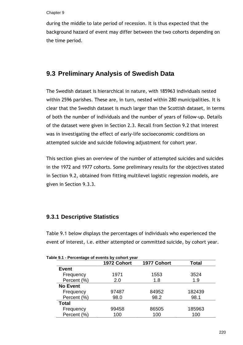
Chapter 9
220
during the middle to late period of recession. It is thus expected that the
background hazard of event may differ between the two cohorts depending on
the time period.
9.3 Preliminary Analysis of Swedish Data
The Swedish dataset is hierarchical in nature, with 185963 individuals nested
within 2596 parishes. These are, in turn, nested within 280 municipalities. It is
clear that the Swedish dataset is much larger than the Scottish dataset, in terms
of both the number of individuals and the number of years of follow-up. Details
of the dataset were given in Section 2.3. Recall from Section 9.2 that interest
was in investigating the effect of early-life socioeconomic conditions on
attempted suicide and suicide following adjustment for cohort year.
This section gives an overview of the number of attempted suicides and suicides
in the 1972 and 1977 cohorts. Some preliminary results for the objectives stated
in Section 9.2, obtained from fitting multilevel logistic regression models, are
given in Section 9.3.3.
9.3.1 Descriptive Statistics
Table 9.1 below displays the percentages of individuals who experienced the
event of interest, i.e. either attempted or committed suicide, by cohort year.
Table 9.1 - Percentage of events by cohort year 1972 Cohort 1977 Cohort Total Event Frequency Percent (%)
1971 2.0
1553 1.8
3524 1.9
No Event Frequency Percent (%)
97487 98.0
84952 98.2
182439
98.1 Total Frequency Percent (%)
99458
100
86505
100
185963
100
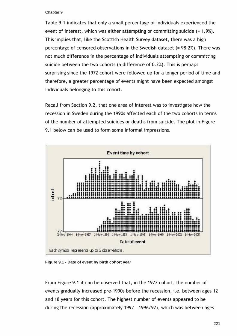
Chapter 9
221
Table 9.1 indicates that only a small percentage of individuals experienced the
event of interest, which was either attempting or committing suicide (= 1.9%).
This implies that, like the Scottish Health Survey dataset, there was a high
percentage of censored observations in the Swedish dataset (= 98.2%). There was
not much difference in the percentage of individuals attempting or committing
suicide between the two cohorts (a difference of 0.2%). This is perhaps
surprising since the 1972 cohort were followed up for a longer period of time and
therefore, a greater percentage of events might have been expected amongst
individuals belonging to this cohort.
Recall from Section 9.2, that one area of interest was to investigate how the
recession in Sweden during the 1990s affected each of the two cohorts in terms
of the number of attempted suicides or deaths from suicide. The plot in Figure
9.1 below can be used to form some informal impressions.
Figure 9.1 - Date of event by birth cohort year
From Figure 9.1 it can be observed that, in the 1972 cohort, the number of
events gradually increased pre-1990s before the recession, i.e. between ages 12
and 18 years for this cohort. The highest number of events appeared to be
during the recession (approximately 1992 – 1996/97), which was between ages

Chapter 9
222
18 and 22 years, before declining in the post-recession period. Individuals in the
1977 cohort were around 13 years old when the recession began. There was a
sharp rise in the number of events halfway through the period of recession
(around 1993/94) for this cohort, i.e. around the ages 15 to 16 years. This would
coincide with the age at which this cohort would be beginning to leave
education to seek employment. The number of events peaked during the second
half of the recession period (around 1995) towards 18 years old. This is around
the time at which all individuals would have left secondary education. There was
a slight decline in the number of events from the end of the recession period;
however, it was not as marked as the decline in the 1972 cohort. This might
suggest that the effects of the recession affected the younger cohort more;
perhaps as they struggled to find employment on leaving education at the end of
the recession period and thus leading to a greater number of attempted suicides
or deaths from suicides.
Some information was also available on variables reflecting the early-life
socioeconomic conditions of the individuals. Table 9.2 below displays the
percentage of events by each early-life socioeconomic risk factor.
The following informal observations can be made from Table 9.2 in terms of the
effect of early-life socioeconomic conditions on the percentage of events. A
greater percentage of females than males experienced the event (difference of
0.9%); the percentage of events was highest for those whose fathers’ social class
was unclassifiable or missing (this category may have included unemployed
persons as unclassifiable); there appeared to be an increasing trend in the
percentage of events as the household income quintile at birth worsened, again
with the highest percentage of events in the ‘missing’ category; a higher
percentage of those in rented accommodation experienced the event than those
in owner occupied accommodation (difference of 1.3%); and the percentage of
events appeared highest among smaller regions, dominated by private
enterprises.

Chapter 9
223
Table 9.2 - Percentage of events by socioeconomic r isk factors Attempted/Committed Suicide
(%)
Sex Male Female
Father’s occupational social class (1980) Employers/Farmers/Entrepreneurs Non-manual workers Manual workers Unclassifiable/Missing
Household income quintile at birth 1 = lowest 2 3 4 5 = highest Missing
Housing tenure at birth Owner occupied Rented
Economic region Metropolitan areas Larger regional centres Smaller regional centres Small regions (mostly private enterprises) Small regions (mostly public sector)
1.5 2.4
1.6 1.3 2.0 3.5
2.2 1.8 1.7 1.8 1.3 4.2
1.5 2.8
2.0 1.8 1.7 2.4 2.0
Table 9.2 suggested that early-life socioeconomic conditions of children may
have an effect on the likelihood of attempting or committing suicide as
measured from age 12 years. It may also have been of interest to investigate
whether the effect of these variables differed by age. This will be considered
during formal analysis by fitting two-way interactions between cohort and each
of the socioeconomic risk factors (and sex). Results from fitting these
interactions will indicate whether the influence of early-life socioeconomic
conditions on the likelihood of attempting or committing suicide varied between
the different cohorts, i.e. the different ages.

Chapter 9
224
9.3.2 Missing Data
There was missing data in the Swedish dataset for all explanatory variables apart
from sex and birth cohort year. Due to the high percentage of missing data for
the variables ‘father’s social class in 1980’ (14% missing), and ‘household income
quintile at birth (4% missing)’, missing or unclassifiable observations for these
variables were included as a separate category in analyses. It is perhaps sensible
to include these as a separate category since it is possible that observations
were classified as missing/unclassifiable as a result of unemployment. This will
be considered further in Section 9.5.2. However, for the variable ‘housing
tenure at birth’ only 0.3% had missing data and thus cases with data missing on
this variable were excluded and not treated as a separate category. There was
also missing data on the higher-level variable, ‘economic region’. Cases with
missing data were excluded from analysis even though a high percentage of
observations (12.3%) were coded as missing. No further information was
available from the data source on why cases with missing data with this variable
were excluded and not coded as a separate category.
Of the 185963 individuals in the Swedish dataset, 12.6% of individuals had
missing data on at least one of the variables ‘economic region’ or ‘housing
tenure at birth’. As discussed above, cases with missing data were excluded
from analysis. This method of case deletion was adopted, as opposed to a
method of imputation, due to time constraints on analyses. Consequences of
ignoring missing data are discussed further in Chapter 10. After excluding cases
with missing data on individual-level variables (housing tenure at birth) there
were 185449 individuals, nested within 2596 parishes, nested within 280
municipalities. However, when excluding cases with missing data on all
individual-level and higher-level variables (housing tenure at birth and economic
region) there were only 162 539 individuals nested within 1988 parishes nested
within 232 municipalities left for analyses.

Chapter 9
225
9.3.3 Results from Preliminary Analyses of Swedish Data
This section presents results obtained from fitting single-level Cox proportional
hazards models (PHM) in SPSS and multilevel logistic regression models in MLwiN.
Results from the Cox PHM and multilevel logistic regression were fitted to gain
an insight into expected results prior to fitting the more complex multilevel
survival models. When fitting the single-level Cox PHM, the response was time
until attempted suicide or death by suicide. Observations were censored if an
individual died from any cause other than suicide or did not experience the
event of interest during follow-up. Single-level models do not account for the
fact that the data are hierarchically structured, consisting of three levels –
individuals nested within parishes nested within municipalities. Instead,
multilevel logistic regression models were fitted to investigate whether there
were any differences in the likelihood of event across the higher levels. For the
multilevel logistic regression, the binary response was of the form ‘individual did
or did not attempt or commit suicide’, as measured from their 12th birthday. A
binomial model with logit link was fitted in MLwiN, and the parameter estimates
were obtained using second-order penalised quasi-likelihood (PQL) estimation.
The outcome was assumed to be Binomially distributed.
Three models (using both a single-level Cox PHM and a multilevel logistic
regression) were fitted to the data. The first contained individual-level variables
only (‘Individual’). The second model added higher-level variables to the model
containing all individual variables (‘Individual+Area’) to see what percentage of
the remaining variation at the higher-levels could be explained by these
variables after adjustment for the individual-level variables. Finally, two-way
interactions between all variables and cohort (‘Full’) were included to
investigate whether the influence of early-life socioeconomic conditions on the
likelihood of attempting or committing suicide varied by age. Results are
displayed in Table 9.3 below. Note that the estimates obtained from the single-
level Cox PHM are log hazard ratios and the estimates obtained from the
multilevel logistic regression model are log odds ratios.

226
Table 9.3 - Results from preliminary analyses of Sw edish data Single-Level Cox PHM Multilevel Logistic Regression
Individual Individual+Area Full Estimate (s.e.) Estimate (s.e.) Estimate (s.e.)
Individual Individual+Area Full Estimate (s.e.) Estimate (s.e.) Estimate (s.e.)
Fixed
Intercept (β0)
Sex Male Female (β1)
Father Soc. Class 1980 Employers etc Non-manual (β2) Manual (β3) Unclassifiable (β4)
Hhold Income Quintile Quintile 1 Quintile 2 (β5) Quintile 3 (β6) Quintile 4 (β7) Quintile 5 (β8) Missing (β9)
Housing Tenure Owner Occupied Rented (β10)
Birth Cohort 1972 1977 (β11)
- - -
0.000** 0.000** 0.000** 0.475 (0.034) 0.496 (0.037) 0.452 (0.049)
0.000** 0.000** 0.000** -0.107 (0.068) -0.102 (0.073) -0.174 (0.092) 0.168 (0.063) 0.169 (0.068) 0.137 (0.087) 0.585 (0.068) 0.563 (0.073) 0.487 (0.092)
0.000** 0.000** 0.000** -0.132 (0.051) -0.142 (0.055) -0.234 (0.072) -0.164 (0.054) -0.164 (0.057) -0.269 (0.076) -0.090 (0.056) -0.095 (0.059) -0.228 (0.079) -0.246 (0.063) -0.285 (0.067) -0.401 (0.086) 0.490 (0.067) 0.463 (0.071) 0.397 (0.094)
0.000** 0.000** 0.000** 0.478 (0.036) 0.484 (0.038) 0.454 (0.050)
0.000** 0.000** 0.000* 0.167 (0.036) 0.149 (0.038) -0.326 (0.155)
-4.463 (0.070) -4.416 (0.080) -4.209 (0.099)
0.000 0.000 0.000 0.481 (0.035) 0.502 (0.037) 0.458 (0.049)
0.000 0.000 0.000 -0.110 (0.069) -0.104 (0.074) -0.178 (0.093) 0.166 (0.064) 0.167 (0.069) 0.135 (0.088) 0.587 (0.069) 0.566 (0.074) 0.491 (0.094)
0.000 0.000 0.000 -0.135 (0.052) -0.145 (0.056) -0.238 (0.073) -0.167 (0.055) -0.166 (0.058) -0.274 (0.077) -0.095 (0.057) -0.098 (0.060) -0.234 (0.081) -0.251 (0.064) -0.288 (0.068) -0.405 (0.088) 0.500 (0.069) 0.473 (0.073) 0.406 (0.097)
0.000 0.000 0.000 0.475 (0.037) 0.484 (0.039) 0.453 (0.051)
0.000 0.000 0.000 -0.026 (0.035) -0.039 (0.038) -0.519 (0.157)

227
Economic Region Metropolitan Larger Regional (β12) Smaller Regional (β13) Private Enterprise(β14) Public Sector (β15)
Cohort*Sex 1972*Male 1977*Female (β16)
Cohort*Soc. Class 1972*Employers etc 1977*Non-manual (β17) 1977*Manual (β18) 1977*Unclass. (β19)
Cohort*Income 1972*Quintile 1 1977*Quintile 2 (β20) 1977*Quintile 3 (β21) 1977*Quintile 4 (β22) 1977*Quintile 5 (β23) 1977*Missing (β24)
Cohort*Housing Tenure 1972*Owner Occupied 1977*Rented (β25)
Cohort*Region 1972*Metropolitan 1977*Larger reg. (β26) 1977*Smaller reg.(β27) 1977*Private (β28) 1977*Public (β29)
Random
Parish Variation(σu2)
Municipal. Variation(σv2)
0.000* 0.000* -0.078 (0.041) -0.104 (0.054) -0.122 (0.058) -0.278 (0.081) 0.148 (0.095) 0.188 (0.119) -0.044 (0.129) -0.230 (0.183) 0.000 0.102 (0.074)
0.000 0.164 (0.151) 0.079 (0.142) 0.181 (0.150)
0.000 0.209 (0.112) 0.240 (0.115) 0.299 (0.120) 0.276 (0.138) 0.147 (0.144)
0.000 0.078 (0.078)
0.000* 0.066 (0.082) 0.345 (0.117) -0.106 (0.196) 0.418 (0.258)
0.000 0.000 -0.075 (0.044) -0.101 (0.056) -0.117 (0.062) -0.274 (0.084) 0.147 (0.100) 0.189 (0.124) -0.031 (0.135) -0.221 (0.188)
0.000 0.102 (0.075)
0.000 0.168 (0.153) 0.080 (0.144) 0.180 (0.152)
0.000 0.212 (0.114) 0.246 (0.117) 0.305 (0.122) 0.280 (0.140) 0.150 (0.148)
0.000 0.081 (0.080)
0.000 0.066 (0.084) 0.347 (0.119) -0.109 (0.200) 0.423 (0.263)
0.022 (0.012) 0.017 (0.011) 0.017 (0.011)
0.000 (0.000) 0.000 (0.000) 0.000 (0.000)

Chapter 9
228
From Table 9.3 it can be observed that, apart from the parameter estimates for
birth cohort year, parameter estimates obtained from the single-level Cox PHM
and the multilevel logistic regression were very similar. However, the parameter
estimates obtained from the single-level Cox PH model and the multilevel
logistic regression model for cohort year were not similar for the ‘Individual’ and
‘Individual+Area’ models. In the single-level model, there were significant
differences in the hazard of event between the two cohorts after adjusting for
other individual- and also other individual- and area-level variables. This effect
was not present in the multilevel logistic regression model.
In the single-level Cox PHM with individual-level covariates only (‘Individual’),
all of the covariates were found to have a highly significant effect on the hazard
of attempting or committing suicide after adjusting for the others. Results
showed the following, after adjusting for each of the other covariates: females
had a significantly higher hazard of event than males; an increasing trend in the
hazard of event was present as fathers’ social class became less
professional/more manual, with those having fathers categorised as
‘unclassifiable or missing’ (which possibly includes unemployed persons) having
the highest hazard of event; there was a general decreasing trend in the hazard
of event as the household income at birth increased (i.e. the direction of the
quintiles ranged 1 to 5), with the ‘missing’ category leading to the highest
hazard of event (again, those classified as missing could be individuals whose
parents were unemployed at the time of birth); those in rented accommodation
at birth had a significantly higher hazard of event later in life than those in
privately owned accommodation; and those in the 1977 cohort had a
significantly higher hazard of event than those in the earlier 1972 cohort. When
the higher-level variable ‘economic region’ was added to this model
(‘Individual+Area’), the individual-level variables remained highly significant and
parameter estimates did not change much. In addition to the individual-level
variables, there was a significant effect of economic region on the hazard of
attempting or committing suicide during follow-up. Finally, as discussed above,
it was of interest to fit two-way interactions between all variables and cohort
(‘Full’) to investigate whether the influence of early-life socioeconomic
conditions on the likelihood of attempting or committing suicide differed
between the two different cohorts. Results from the single-level PHM indicated
Chapter 9
229
that the only significant interaction was between cohort year and economic
region. Results suggest that the effect of economic region on the hazard of
event was generally stronger for those born in 1977. This may coincide with the
impression that the recession had a longer-lasting effect on the younger 1977
cohort. If such individuals were struggling to find employment post-recession,
then it is possible that they were unable to move away from economic regions
that could be having a damaging effect on their health.
As noted above, apart from the variable ‘cohort’, parameter estimates for the
covariates in the ‘Individual’ and ‘Individual+Area’ models were similar when
using the multilevel logistic regression model to when the single-level Cox PHM
was used. However, as the data were hierarchical, with individuals nested within
parishes nested within municipalities, it was more appropriate to use a
multilevel model. This allowed the variation in the hazard of attempting or
committing suicide to be partitioned into that attributable to differences
between individuals and that attributable to differences between municipalities
and parishes. In the ‘Individual’ multilevel logistic regression model, taking the
antilogit function of the intercept indicated that, following adjustment for all
individual-level covariates, the probability of attempting or committing suicide
for a person with baseline characteristics in the average district within
municipality was 0.011. There was no variation in the hazard of event at the
highest level, i.e. between municipalities, and less than 1% (=0.66%) of the total
variation was attributable to differences between parishes within municipalities.
Adding economic region to the model (i.e. the ‘Individual+ Area’ model)
explained 23% of the variation between parishes within municipalities. No
further variation at the parish (within municipality) level was explained by
adding two-way individual-level and cross-level interactions between each
variable and cohort year. Parameter estimates for all two-way interactions
obtained from the multilevel logistic regression model were similar to those
obtained from the single-level Cox PHM. This suggests that the only significant
two-way interaction was the cross-level interaction between birth cohort year
and economic region.

Chapter 9
230
9.3.4 Summary of Preliminary Analyses of Swedish Da ta
One objective of the Swedish dataset was to investigate the association between
early-life socioeconomic conditions and the hazard of attempting or committing
suicide, as measured from an individual’s 12th birthday. Multilevel models must
be used to account for the hierarchical nature of the data – individuals within
parishes within municipalities.
Before fitting the more complex multilevel survival models, some preliminary
analysis of the dataset, using single-level proportional hazards models and
multilevel logistic regression models, was carried out in order to gain an insight
into expected results. Results indicated that there were significant additive
effects of sex and various measures of early-life socioeconomic conditions on the
hazard or odds of event. There was also some evidence of a significant cross-
level interaction between birth cohort year and economic region. The multilevel
logistic regression model showed that there was no variation in the hazard of
event at the municipality level, and less than 1% was attributable to differences
between parishes within municipalities. It is expected that similar results will be
observed when fitting multilevel survival models.
9.4 Fitting Multilevel Survival Models to the Swedi sh
Dataset
As discussed in previous chapters, the proportional hazards model (PHM) is one
of the most commonly used continuous-time models for modelling survival data.
The single-level PHM may be extended to include random effects yielding a
multilevel model. MLwiN is able to fit multilevel continuous-time proportional
hazards models via a multilevel Poisson model fitted to a person-period dataset.
As creation of the person-period dataset leads to an expansion in the size of the
original dataset, computational problems can arise if the original dataset is large
to begin with and/or if individuals are followed up for a long period of time.
Thus, it is of interest to investigate alternative ways of fitting multilevel survival
Chapter 9
231
models to large datasets since it is clear that continuous-time models can be
problematic.
Previous chapters considered three possible alternatives to fitting continuous-
time multilevel models in MLwiN. These included fitting discrete-time models in
MLwiN, aggregating data according to covariates and fitting continuous- and
discrete-time models to the aggregated data and fitting frailty models in
WinBUGS. The three methods were fitted to a moderately-sized Scottish dataset
in order to test their suitability as an alternative to the continuous-time models
fitted in MLwiN. This section will now consider whether the alternative methods
are still appropriate when fitted to a much larger Swedish dataset. The dataset
is large in terms of the number of individuals and the period of follow-up.
9.4.1 Multilevel Continuous-Time Survival Models
It was of interest to investigate whether MLwiN would be able to estimate a
continuous-time proportional hazards model, fitted via a Poisson model, to the
large Swedish dataset. First, the person-period dataset had to be created. The
‘SURV’ command in MLwiN is used to perform the data expansion. However, the
Swedish dataset proved to be much too large to use the ‘SURV’ command in
order to create the expanded dataset when time was treated as a continuous
variable, i.e. measured in days. As the person-period dataset could not be
created, multilevel PH models, fitted via Poisson models in MLwiN, could not be
implemented in this package. Recall also that, due to the high percentage of
censored observations in the Swedish dataset (98%), the accelerated lifetime
(log-duration) model, which does not require any data expansion, could not be
used. This is because of the tendency of the quasi-likelihood estimation
procedure to break down for this model in the presence of many censored
observations. Furthermore, as there were three hierarchical levels in the
Swedish data, the only other readily available statistical package that could be
used to fit multilevel survival models is WinBUGS (refer to Section 5.3.2). Fitting
multilevel survival (frailty) models in WinBUGS is considered in Section 9.4.4.

Chapter 9
232
9.4.2 Multilevel Discrete-time Survival Models
Multilevel discrete-time models (fitted in MLwiN) were found to be a useful
alternative to fitting continuous-time models in MLwiN when tested on the
moderately-sized Scottish Health Survey dataset. Time was divided into short
intervals, of either equal or varying length, leading to a reduction in the number
of risk sets and hence a reduction in the size of the expanded person-period
dataset. Discrete-time models were easily implemented using multilevel logistic
regression models fitted to the person-period dataset. It was of interest to see
how well these models would perform when fitted to a much larger dataset.
Various groupings were considered when dividing up time to form the discrete-
time intervals. It was of interest to investigate the largest number of discrete-
time intervals that MLwiN would allow before the person-period dataset became
too large and estimating the models became problematic. Conversely, it was
also of interest to determine the smallest number of discrete-time intervals
permitted without losing precision by having wide intervals.
Table 9.4 below summarises the various attempts at dividing up time. It displays
whether time was divided into intervals of equal or varied lengths according to
when each event occurred, how many risk sets resulted from the division and
the size of the expanded dataset for each particular division. Finally, it indicates
whether each of the three models described in Section 9.3.3, i.e. the
‘Individual’, ‘Individual+Area’ and ‘Full’ models, as well as a baseline model
containing no covariates, could be estimated in MLwiN. Information on the
estimation procedure used is also displayed. Parameter estimates for the three
models fitted to the smallest and largest datasets resulting from the various
groupings are then displayed in Table 9.7. Checks of proportionality assumptions
are included in Appendix 6.
Table 9.4 shows that grouping time into year-long intervals led to an expanded
dataset that was too large to allow the estimation of models. The expanded
dataset for this particular grouping of time consisted of 3801822 observations
within individuals – twice as many as the moderately sized Scottish Health Survey
dataset which consisted of approximately 1.9 million observations within
individuals in the continuous-time case. Further grouping of time into intervals

Chapter 9
233
of length 2 years halved the size of the expanded dataset from when time was
grouped in years; however, estimation of models was still problematic and only
the baseline model, with no covariates, included could be estimated.
There were four alternative groupings for intervals of varied length considered in
Table 9.4. The groupings were defined according to days when clusters of events
occurred when looking at dotplots of the event/survival times. Groupings for the
expanded dataset with 3 risk sets are given in Table 9.5 and in Table 9.6 for the
expanded dataset with 7 risk sets. Groupings for the other expanded datasets
can be found in Appendix 5. It can be observed that, as the number of risk sets
decreased, i.e. the lengths of the intervals became longer, the size of the
expanded dataset also decreased.

234
Table 9.4 - Dividing time in the Swedish dataset
Division No. of
Risk Sets Size of
Expanded Dataset
Baseline Individual Individual+Area Full
Equal year-long intervals
Equal two-year long intervals
Varied - defined by events
Varied - defined by events
Varied - defined by events
Varied - defined by events
23
12
10
7
5
3
3 801 822
1 950 471
1 668 284
1 202 560
921 279
553 652
- - - -
Polynomial PQL2
Blocking Factors PQL2 PQL2 - PQL2
Blocking Factors PQL2 PQL2 PQL2 PQL2
Blocking Factors PQL2 PQL2 PQL2 PQL2
Blocking Factors PQL2 PQL2 PQL2 PQL2

Chapter 9
235
Table 9.5 - Discrete-time grouping for expanded dat aset with 3 risk sets Time Interval Grouping
1 2 3 4
Day 0 – day 2700 Day 2701 – day 4500 Day 4501 – day 8373 Day 8374 – day 8500
Table 9.6 - Discrete-time grouping for expanded dat aset with 7 risk sets Time Interval Grouping
1 2 3 4 5 6 7 8
Day 0 – day 1700 Day 1701 – day 2700 Day 2701 – day 3500 Day 3501 – day 4500 Day 4501 – day 5900 Day 5901 – day 6900 Day 6901 – day 8373 Day 8374 – day 8500
Table 9.5 displays the division of time for the expanded dataset with 3 risk sets.
Note that, although there were 4 distinct time intervals, the last time interval
contains only censored observations (since the last event occurred at 8373 days
from 12th birthday), and therefore was not included as a risk set since no events
occurred during that interval. Note that the last event for those in the 1977
cohort was 6502 days from 12th birthday. Similarly, for the expanded dataset
with 7 risk sets (Table 9.6), there were 8 distinct time intervals; however, the
last time interval contained censored observations only and thus was not
included as a risk set.
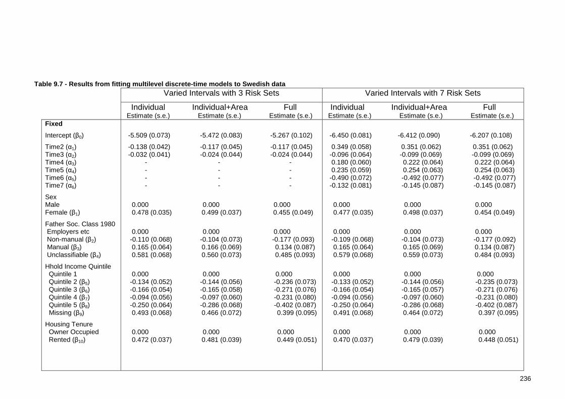
236
Table 9.7 - Results from fitting multilevel discret e-time models to Swedish data Varied Intervals with 3 Risk Sets Varied Intervals with 7 Risk Sets
Individual Individual+Area Full Estimate (s.e.) Estimate (s.e.) Estimate (s.e.)
Individual Individual+Area Full Estimate (s.e.) Estimate (s.e.) Estimate (s.e.)
Fixed
Intercept (β0)
Time2 (α1) Time3 (α2) Time4 (α3) Time5 (α4) Time6 (α5) Time7 (α6)
Sex Male Female (β1)
Father Soc. Class 1980 Employers etc Non-manual (β2) Manual (β3) Unclassifiable (β4)
Hhold Income Quintile Quintile 1 Quintile 2 (β5) Quintile 3 (β6) Quintile 4 (β7) Quintile 5 (β8) Missing (β9)
Housing Tenure Owner Occupied Rented (β10)
-5.509 (0.073) -5.472 (0.083) -5.267 (0.102)
-0.138 (0.042) -0.117 (0.045) -0.117 (0.045) -0.032 (0.041) -0.024 (0.044) -0.024 (0.044) - - - - - - - - - - - -
0.000 0.000 0.000 0.478 (0.035) 0.499 (0.037) 0.455 (0.049)
0.000 0.000 0.000 -0.110 (0.068) -0.104 (0.073) -0.177 (0.093) 0.165 (0.064) 0.166 (0.069) 0.134 (0.087) 0.581 (0.068) 0.560 (0.073) 0.485 (0.093)
0.000 0.000 0.000 -0.134 (0.052) -0.144 (0.056) -0.236 (0.073) -0.166 (0.054) -0.165 (0.058) -0.271 (0.076) -0.094 (0.056) -0.097 (0.060) -0.231 (0.080) -0.250 (0.064) -0.286 (0.068) -0.402 (0.087) 0.493 (0.068) 0.466 (0.072) 0.399 (0.095)
0.000 0.000 0.000 0.472 (0.037) 0.481 (0.039) 0.449 (0.051)
-6.450 (0.081) -6.412 (0.090) -6.207 (0.108)
0.349 (0.058) 0.351 (0.062) 0.351 (0.062) -0.096 (0.064) -0.099 (0.069) -0.099 (0.069) 0.180 (0.060) 0.222 (0.064) 0.222 (0.064) 0.235 (0.059) 0.254 (0.063) 0.254 (0.063) -0.490 (0.072) -0.492 (0.077) -0.492 (0.077) -0.132 (0.081) -0.145 (0.087) -0.145 (0.087)
0.000 0.000 0.000 0.477 (0.035) 0.498 (0.037) 0.454 (0.049)
0.000 0.000 0.000 -0.109 (0.068) -0.104 (0.073) -0.177 (0.092) 0.165 (0.064) 0.165 (0.069) 0.134 (0.087) 0.579 (0.068) 0.559 (0.073) 0.484 (0.093)
0.000 0.000 0.000 -0.133 (0.052) -0.144 (0.056) -0.235 (0.073) -0.166 (0.054) -0.165 (0.057) -0.271 (0.076) -0.094 (0.056) -0.097 (0.060) -0.231 (0.080) -0.250 (0.064) -0.286 (0.068) -0.402 (0.087) 0.491 (0.068) 0.464 (0.072) 0.397 (0.095)
0.000 0.000 0.000 0.470 (0.037) 0.479 (0.039) 0.448 (0.051)

237
Birth Cohort 1972 1977 (β11)
Economic Region Metropolitan Larger Regional (β12) Smaller Regional (β13) Private Enterprise(β14) Public Sector (β15)
Cohort*Sex 1972*Male 1977*Female (β16)
Cohort*Soc. Class 1972*Employers etc 1977*Non-manual (β17) 1977*Manual (β18) 1977*Unclass. (β19)
Cohort*Income 1972*Quintile 1 1977*Quintile 2 (β20) 1977*Quintile 3 (β21) 1977*Quintile 4 (β22) 1977*Quintile 5 (β23) 1977*Missing (β24)
Cohort*Housing Tenure 1972*Owner Occupied 1977*Rented (β25)
Cohort*Region 1972*Metropolitan 1977*Larger reg. (β26) 1977*Smaller reg.(β27) 1977*Private (β28) 1977*Public (β29)
0.000 0.000 0.000 -0.025 (0.035) -0.038 (0.037) -0.514 (0.156)
0.000 0.000 -0.074 (0.043) -0.100 (0.056) -0.116 (0.061) -0.271 (0.083) 0.147 (0.099) 0.189 (0.123) -0.032 (0.133) -0.219 (0.187) 0.000 0.102 (0.075)
0.000 0.166 (0.152) 0.080 (0.143) 0.180 (0.151)
0.000 0.210 (0.113) 0.242 (0.116) 0.301 (0.121) 0.277 (0.139) 0.150 (0.146)
0.000 0.080 (0.079)
0.000 0.064 (0.083) 0.344 (0.118) -0.108 (0.198) 0.418 (0.261)
0.000 0.000 0.000 0.103 (0.036) 0.087 (0.038) -0.389 (0.156)
0.000 0.000 -0.074 (0.043) -0.100 (0.056) -0.116 (0.061) -0.270 (0.083) 0.147 (0.098) 0.189 (0.123) -0.032 (0.133) -0.218 (0.187)
0.000 0.102 (0.074)
0.000 0.166 (0.152) 0.080 (0.142) 0.179 (0.151)
0.000 0.210 (0.113) 0.242 (0.116) 0.301 (0.120) 0.277 (0.139) 0.150 (0.145)
0.000 0.080 (0.079)
0.000 0.064 (0.083) 0.343 (0.117) -0.108 (0.197) 0.417 (0.260)
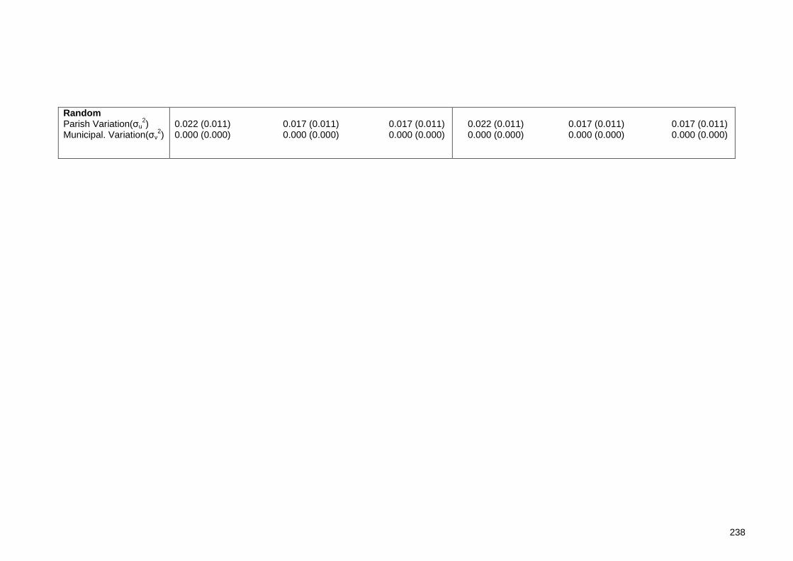
238
Random Parish Variation(σu
2) Municipal. Variation(σv
2)
0.022 (0.011) 0.017 (0.011) 0.017 (0.011) 0.000 (0.000) 0.000 (0.000) 0.000 (0.000)
0.022 (0.011) 0.017 (0.011) 0.017 (0.011) 0.000 (0.000) 0.000 (0.000) 0.000 (0.000)
Chapter 9
239
Table 9.7 displays results obtained from fitting the three models (‘Individual’,
‘Individual+Area’ and ‘Full’) to the expanded dataset with 3 risk sets and the
expanded dataset with 7 risk sets. It was discussed above that it was of interest
to compare parameter estimates from the models fitted to the smallest and
largest expanded datasets resulting from the various groupings of time. This was
in order to determine whether precision had been lost by having a fewer number
of longer time intervals. The fewer the number of time intervals, the smaller the
size of the expanded dataset, meaning that models can be estimated in a
shorter time. The person-period dataset with 7 risk sets was chosen to compare
results from the person-period dataset with 3 risk sets. This was because it was
the largest expanded dataset that allowed estimation of all three models (see
Table 9.4). Blocking factors were used to estimate the baseline hazard function
in these models. A polynomial function could also have been used for the
expanded dataset with 7 risk sets of varied lengths to reduce the number of
nuisance parameters to be estimated.
The first aspect to be considered from Table 9.7 was whether the three models,
fitted to both of the different sizes of expanded dataset, yielded similar
parameter estimates. Considering just the ‘Individual’ and ‘Individual+Area’
models, it was observed that the parameter estimates for all covariates, apart
from ‘cohort’, were very similar for the two different datasets. However, in the
‘Individual’ and ‘Individual+Area’ models fitted to the expanded dataset with 3
risk sets, there was no significant effect of cohort on the hazard of attempting
or committing suicide following adjustment for the other covariates. This was
not the case for the same models fitted to the expanded dataset with 7 risk sets.
In this case, there was a significant effect of cohort, with those born in 1977
having a significantly higher hazard of event during follow-up than those born in
1972, after adjusting for the other covariates. This suggested that, when time
was divided into intervals of longer length, the effect of cohort on the hazard of
event was being lost. This will be considered below.
The estimates of the alpha parameters in the models indicated the change in the
baseline hazard as time increased, i.e. as individuals get older. The baseline
hazard was fitted using blocking factors, i.e. dummy variables, where the
baseline hazard of event in each risk set was compared to the baseline hazard in
the first risk set. The intercept, β0, denotes the hazard of event in the first risk

Chapter 9
240
set. For the models fitted to the expanded dataset with 3 risk sets, the
parameter estimates for alpha indicated that there was a significantly lower
hazard of event during the second risk set compared to the first risk set, i.e. a
lower hazard of event when individuals were aged 19-24 years than when they
were aged 12-19 years. There were no significant differences in the baseline
hazard between the third and first risk set, i.e. between ages 24-34 years (24-29
years for those in the 1977 cohort) and 12-19 years. This was not what was
observed from the models fitted to the expanded dataset with 7 risk sets.
Instead it can be seen that, compared to the first risk set, i.e. aged 12-16 years,
there was a significantly higher hazard of event in the second risk set (aged 16-
19 years), the fourth risk set (aged 21-24 years) and the fifth risk set (aged 24-28
years). In addition, there was a significantly lower hazard of event in the sixth
risk set (age 28-30 for 1972 cohort and 28-29 for the 1977 cohort) than in the
first risk set. These differences were not observed when the broader groupings
of time were used, i.e. when there were only 3 risk sets.
There was no clear evidence of any two-way interactions between cohort year
and the socioeconomic variables in the ‘Full’ models fitted to the expanded
dataset with 3 or with 7 risk sets.
Parameter estimates from the multilevel discrete-time survival models were
compared to those obtained from the single-level PHM and the multilevel logistic
regression. Parameter estimates for the ‘Individual’, ‘Individual+Area’ and the
‘Full’ models fitted using the three different methods (single-level PHM,
multilevel logistic and multilevel survival) were similar for all parameters apart
from ‘cohort’. Parameter estimates for ‘cohort’ obtained from the single-level
PH models were similar to those obtained from the multilevel discrete-time
models fitted to the expanded dataset with 7 risk sets. However, parameter
estimates obtained for this variable from the multilevel logistic regression
models were more similar to those obtained from the multilevel discrete-time
model fitted to the expanded dataset with 3 risk sets. This demonstrated again
that the parameter estimate for ‘cohort’ was affected by the way time was
divided. This result is not unexpected since it is known that parameter estimates
of coefficients depend on the length of the time interval when the logistic model
is used to fit the discrete-time hazard model [156, 157]. Allison [156] and
Petersen [157] gave a detailed overview of this problem and discussed that, if

Chapter 9
241
the width of the time interval is small (and hence the probability of an event in
each time interval is small), then the logistic model converges to the
proportional hazards model, and coefficients obtained from using a discrete-
time model will be quite similar to those obtained from a continuous-time
model. Also, if the probability of event is small, only the intercept term depends
on the length of the time interval, with changes in the time unit tending to have
no influence on the other coefficients. Petersen and Allison offered some
possible solutions to overcome the problem of the dependence of coefficients on
the length of time intervals. Petersen discussed an estimator which could be
used to adjust for time aggregation bias. Alternatively, both Allison & Petersen
discussed that a complementary log-log link function could be used instead of
the logistic regression function. They discussed how the complementary log-log
model is unaffected by the length of time intervals, and would provide
consistent estimators of the continuous-time proportional hazards model,
regardless of the length of time intervals.
With the knowledge that parameter estimates for the regression parameters can
be affected by the length of time interval, it is somewhat interesting that only
the coefficients for the variable ‘cohort’ (after accounting for the other
variables in the model) seemed to be affected by having a smaller number of
risk sets of longer length. This indicates that the effect of cohort on the hazard
of event depended on the length of time interval used, suggesting an interaction
between time and cohort. With this in mind, the next step in analysis would be
to include a two-way interaction between time and cohort to investigate
whether the effect of time on the hazard of event differs by cohort. It seemed
reasonable to assume that the parameter estimates obtained from the models
fitted to the expanded dataset with 7 risk sets were more accurate than those
obtained from the models fitted to the expanded dataset with 3 risk sets. This
view was held since the former obtained estimates which were more similar to
those produced by the single-level proportional hazards model, where time was
treated as a continuous variable. It should be noted also that the same three
models were fitted to an expanded dataset containing 5 risk sets (results
displayed in Appendix 7); however, the estimates of cohort in each of the
models were more similar to those obtained from the models fitted to the
expanded dataset with 3 risk sets, thus suggesting that the groupings of time

Chapter 9
242
used in this case were still too large to provide consistent estimators of the
proportional hazards parameters.
From fitting three different models to the expanded datasets, i.e. ‘Individual’,
‘Individual+Area’ and ‘Full’, it was observed that the ‘Individual+Area’ model,
which included all individual- and higher-level additive effects, was the most
appropriate model. This was because it explained the largest amount of
variation in the hazard of event at the higher level, and also because there were
no significant two-way interactions between cohort year and any of the other
socioeconomic variables. Therefore, a two-way interaction between time and
cohort was included in the ‘Individual+Area’ model fitted to the expanded
dataset with 7 risk sets. Results are displayed in Table 9.8 below.
Results from Table 9.8 for the two-way interaction between time and cohort
indicated that, after adjusting for early-life socioeconomic risk factors, the
hazard of attempting or committing suicide in the third risk set (i.e. aged 19-21)
and in the sixth risk set (i.e. aged 28-30 for those in the 1972 cohort and 28-29
for those in the 1977 cohort) compared to the first risk set was significantly
lower for those in the 1977 cohort than those in the 1972 cohort. This difference
could reflect the effect of the recession on the hazard of event; those in the
1972 cohort would have been trying to find employment in the middle of the
recession when aged 19-21 years, whereas the recession had passed by the time
those in the 1977 cohort were aged 19-21 years and were perhaps seeking
employment. The difference in the hazard of event during the 6th risk set
between the two cohorts possibly just reflected the end of follow-up for those in
the 1977 cohort, thus censoring any remaining individuals. As expected, the
parameter estimate for the time*cohort interaction in the seventh risk set (i.e.
β22) was zero, simply indicating the longer period of follow-up for those in the
1972 cohort. Finally, parameter estimates and estimated standard errors for all
additive effects remained unchanged as a result of adding the interaction
between time and cohort. Addition of this term did not explain any more of the
variation in the hazard of event at the parish level.

Chapter 9
243
Table 9.8 - Results from investigating the effect o f cohort
Estimate (s.e.)
Fixed
Intercept (β0)
Time 1 Time2 (α1) Time3 (α2) Time4 (α3) Time5 (α4) Time6 (α5) Time7 (α6)
Sex Male Female (β1)
Father Soc. Class 1980 Employers etc Non-manual (β2) Manual (β3) Unclassifiable (β4)
Hhold Income Quintile Quintile 1 Quintile 2 (β5) Quintile 3 (β6) Quintile 4 (β7) Quintile 5 (β8) Missing (β9)
Housing Tenure Owner Occupied Rented (β10)
Birth Cohort 1972 1977 (β11)
Economic Region Metropolitan Larger Regional (β12) Smaller Regional (β13) Private Enterprise(β14) Public Sector (β15)
Time*Cohort 1972*Time 1 (β16) 1977*Time 2 (β17) 1977*Time 3 (β18) 1977*Time 4 (β19) 1977*Time 5 (β20) 1977*Time 6 (β21) 1977*Time 7 (β22)
Random
Parish Variation(σu2)
Municipal. Variation(σv2)
-6.506 (0.101)
0.000 0.468 (0.086) 0.055 (0.095) 0.298 (0.090) 0.179 (0.092) -0.091 (0.099) -0.052 (0.098)
0.000 0.498 (0.037)
0.000 -0.104 (0.073) 0.165 (0.069) 0.559 (0.073)
0.000 -0.144 (0.056) -0.165 (0.057) -0.097 (0.060) -0.286 (0.068) 0.464 (0.072)
0.000 0.479 (0.039)
0.000 0.278 (0.095)
0.000 -0.074 (0.043) -0.116 (0.061) 0.147 (0.098) -0.032 (0.133)
0.000 -0.244 (0.124) -0.326 (0.138) -0.154 (0.127) 0.141 (0.127) -1.032 (0.166) 0.000 (0.000)
0.017 (0.011) 0.000 (0.000)

Chapter 9
244
9.4.3 Grouping According to Covariates
If individuals nested within the same higher-level units have the same values for
covariates included in a particular model, then it is clear that these individuals
are at risk of experiencing the event of interest at the same time. The data for
these individuals can be aggregated so that only one line of data represents all
such individuals, thus leading to a reduction in the size of the expanded person-
period dataset. This so-called ‘grouping according to covariates’ method was
found to successfully reduce the size of the expanded Scottish Health Survey
dataset, especially when time was treated as a discrete variable. It was
therefore of interest to investigate if this method performed as well when fitted
to the much larger Swedish dataset.
There were a number of points to consider before applying this method to the
Swedish dataset. Firstly, since the data aggregation must be carried out using
the expanded dataset, time could only be treated as a discrete variable since
the Swedish dataset was much too large to expand in MLwiN when time was
being treated as continuous. Secondly, in the Scottish dataset, individuals were
nested within postcode-sectors only, but in the Swedish dataset, there is a
further higher level, with individuals being nested within parishes, which are in
turn nested within municipalities. However, as parishes are nested within
municipalities, the grouping will be the same as it would be if municipalities
were ignored.
To apply this method to the Swedish dataset, the expanded dataset with 7 risk
sets was used for aggregation. Four models were fitted to the expanded dataset
after aggregation; the ‘Individual’ model, the ‘Individual+Area’ model, the ‘Full’
model and the ‘Individual+Area’ model which also included a two-way
interaction between time and cohort. To fit these models, two aggregated
datasets had to be created. The first aggregated data for individuals in the same
parish and municipality with the same values for individual-level covariates and
the second aggregated data for individuals within the same parish and
municipality with the same values for individual-level and higher-level
covariates. Although time was discrete, Poisson models were used for reasons
discussed in Section 8.2.2, and the logarithm of the cell size was used as the

Chapter 9
245
offset. Blocking factors were used to model the baseline hazard function. All
models were estimated using second-order PQL. Table 9.9 displays the
percentage reduction in the expanded dataset with 7 risk sets after aggregation.
Recall, from Table 9.4, that the size of the expanded dataset with 7 risk sets
was 1 202 560. Results are displayed in Table 9.10 below, and parameter
estimates should be compared to those in Tables 9.7 and 9.8.
Table 9.9 - Percentage reduction in expanded datase t when grouping according to covariates
Covariate Grouping Size of New Dataset % Reduction
Individual 531 726 56%
Individual+Area 531 726 56%
Table 9.9 shows that when data for individuals nested in the same parish within
municipality were aggregated according to values of individual-level covariates,
the reduction in size from the expanded dataset with 7 risk sets was 56%.
Sections 8.2.3 and 8.4 discussed how the percentage reduction would decrease
as the number of covariates to be grouped on increased; however, it can be seen
from Table 9.9 that this was not the case when a further higher-level covariate
was added to the list of covariates to be grouped on. The higher-level variable
that was added, economic region, indicates what type of area the parish within
municipality is; therefore, it is expected that all individuals in the same parish
within municipality would have the same categorical value for this variable. As a
result, it was not surprising that adding this variable to the list of covariates to
be grouped on had no effect on the percentage reduction.

246
Table 9.10 - Results from grouping according to cov ariates with Swedish data Varied Intervals with 7 Risk Sets
Individual Individual+Area Full Individual+Area+Time*Cohort Estimate (s.e.) Estimate (s.e.) Estimate (s.e.) Estimate (s.e.)
Fixed
Intercept (β0)
Time2 (α1) Time3 (α2) Time4 (α3) Time5 (α4) Time6 (α5) Time7 (α6)
Sex Male Female (β1)
Father Soc. Class 1980 Employers etc Non-manual (β2) Manual (β3) Unclassifiable (β4)
Hhold Income Quintile Quintile 1 Quintile 2 (β5) Quintile 3 (β6) Quintile 4 (β7) Quintile 5 (β8) Missing (β9)
Housing Tenure Owner Occupied Rented (β10)
-6.452 (0.080) -6.415 (0.090) -6.209 (0.108) -6.508 (0.101)
0.348 (0.058) 0.349 (0.062) 0.349 (0.062) 0.466 (0.086) -0.095 (0.064) -0.098 (0.069) -0.098 (0.069) 0.055 (0.094) 0.180 (0.060) 0.221 (0.063) 0.221 (0.063) 0.296 (0.089) 0.235 (0.059) 0.253 (0.063) 0.253 (0.063) 0.178 (0.092) -0.488 (0.072) -0.490 (0.077) -0.490 (0.077) -0.090 (0.098) -0.131 (0.081) -0.144 (0.086) -0.144 (0.086) -0.052 (0.097)
0.000 0.000 0.000 0.000 0.474 (0.035) 0.494 (0.037) 0.452 (0.049) 0.494 (0.037)
0.000 0.000 0.000 0.000 -0.106 (0.068) -0.100 (0.073) -0.176 (0.092) -0.100 (0.073) 0.168 (0.064) 0.169 (0.069) 0.134 (0.087) 0.169 (0.069) 0.581 (0.068) 0.561 (0.073) 0.482 (0.093) 0.561 (0.073)
0.000 0.000 0.000 0.000 -0.134 (0.052) -0.144 (0.055) -0.234 (0.072) -0.144 (0.055) -0.165 (0.054) -0.164 (0.057) -0.269 (0.076) -0.164 (0.057) -0.093 (0.056) -0.097 (0.059) -0.229 (0.080) -0.097 (0.059) -0.249 (0.064) -0.285 (0.068) -0.400 (0.087) -0.285 (0.068) 0.490 (0.067) 0.464 (0.071) 0.394 (0.095) 0.464 (0.071)
0.000 0.000 0.000 0.000 0.468 (0.037) 0.477 (0.039) 0.447 (0.051) 0.477 (0.039)

247
Birth Cohort 1972 1977 (β11)
Economic Region Metropolitan Larger Regional (β12) Smaller Regional (β13) Private Enterprise(β14) Public Sector (β15)
Cohort*Sex 1972*Male 1977*Female (β16)
Cohort*Soc. Class 1972*Employers etc 1977*Non-manual (β17) 1977*Manual (β18) 1977*Unclass. (β19)
Cohort*Income 1972*Quintile 1 1977*Quintile 2 (β20) 1977*Quintile 3 (β21) 1977*Quintile 4 (β22) 1977*Quintile 5 (β23) 1977*Missing (β24)
Cohort*Housing Tenure 1972*Owner Occupied 1977*Rented (β25)
Cohort*Region 1972*Metropolitan 1977*Larger reg. (β26) 1977*Smaller reg.(β27) 1977*Private (β28) 1977*Public (β29)
0.000 0.000 0.000 0.000 0.102 (0.036) 0.086 (0.038) -0.395 (0.156) 0.276 (0.095)
0.000 0.000 0.000 -0.074 (0.043) -0.099 (0.056) -0.074 (0.043) -0.115 (0.061) -0.270 (0.083) -0.115 (0.061) 0.147 (0.098) 0.188 (0.122) 0.147 (0.098) -0.032 (0.133) -0.218 (0.186) -0.032 (0.133)
0.000 0.098 (0.074)
0.000 0.176 (0.152) 0.091 (0.143) 0.192 (0.151)
0.000 0.204 (0.112) 0.239 (0.116) 0.298 (0.120) 0.275 (0.139) 0.154 (0.144)
0.000 0.077 (0.079)
0.000 0.064 (0.083) 0.342 (0.117) -0.107 (0.197) 0.416 (0.259)

248
Time*Cohort 1972*Time 1 (β30) 1977*Time 2 (β31) 1977*Time 3 (β32) 1977*Time 4 (β33) 1977*Time 5 (β34) 1977*Time 6 (β35) 1977*Time 7 (β36)
Random Parish Variation(σu
2) Municipal. Variation(σv
2)
0.000 -0.242 (0.123) -0.324 (0.138) -0.152 (0.127) 0.141 (0.126) -1.029 (0.166) 0.000 (0.000)
0.021 (0.011) 0.016 (0.011) 0.016 (0.011) 0.016 (0.011) 0.000 (0.000) 0.000 (0.000) 0.000 (0.000) 0.000 (0.000)

Chapter 9
249
From examining parameter estimates for the ‘Individual’ model in Table 9.10
and comparing them to results obtained from fitting the same model before
aggregation of the dataset with 7 risk sets (Table 9.7), it can be seen that
parameter estimates and estimated standard errors, of both the fixed and
random effects, were either identical or very similar following data aggregation
to what they were prior to aggregating the data. This was also true of the
‘Individual+Area’ model. When two-way interactions between birth cohort year
and the socioeconomic risk factors (and sex) were added to the model fitted to
the aggregated dataset with 7 risk sets (i.e. the ‘Full’ model), parameter
estimates for the interaction terms were not as similar to those obtained from
the same model fitted to the dataset with 7 risk sets before aggregation as they
had been for the main effects. However, the differences were not especially
large, and 95% confidence intervals (not displayed here) for the parameter
estimates of the interaction terms in the model fitted to the aggregated dataset
contained the estimates of the respective parameters obtained from fitting the
same model to the same dataset before aggregation. Finally, when comparing
results from the ‘Individual+Area+Time*Cohort’ model (Table 9.10), it can be
seen that parameter estimates and estimated standard errors of all fixed effects
and random effects were either identical or very similar to those obtained for
the same model fitted to the same dataset before aggregation (results in Table
9.8). Recall that, this model included all socioeconomic risk factors (and sex)
and a two-way interaction between birth cohort year and the dummy variables
for time (used to estimate the baseline hazard function).
This section has shown that the grouping according to covariates method has
performed well, even on a larger dataset with a longer period of follow-up time,
as compared to the Scottish ‘training’ dataset. This method can be deemed
successful for the Swedish dataset since aggregating the person-period dataset
led to a high percentage reduction (56%) in the size of the same dataset before
aggregation. More importantly, however, parameter estimates were either
identical or very similar to those obtained before aggregation. A possible
explanation as to why this method has been successful for this dataset may be
the large number of individuals living within each parish. After deletion of all
individuals with missing data, there were approximately 82 individuals per parish
on average. As discussed in Section 8.4, for a higher level unit consisting of a
Chapter 9
250
larger number of individuals, there is a greater chance that more of these
individuals will share the same values for the covariates to be grouped on. This
could be why the percentage reduction in the expanded dataset with 7 risk sets
following aggregation was so large at over a fifty percent reduction.
9.4.4 Bayesian Frailty Models
As discussed throughout this thesis, fitting multilevel proportional hazards
models in MLwiN, whether they are continuous-time models or discrete-time
(proportional odds) models, requires the creation of a person-period dataset.
This inevitably leads to an expansion in the size of the original dataset. One
alternative to fitting multilevel survival models in MLwiN, as reviewed in Section
7.4, is to adopt a Bayesian approach. Although the Poisson model used to
estimate the proportional hazards model in MLwiN can be fitted using a Bayesian
approach, MCMC methods used to estimate the Bayesian model can result in long
computing times. Instead, the so-called ‘shared frailty’ model can be used,
where the frailty term, equal to the exponential of the random effects, wj =
exp(uj), accounts for the clustering of individuals within higher-level units.
WinBUGS can be used to fit the shared-frailty model. An additive frailty model is
adopted by WinBUGS and a Weibull distribution is assumed for the survivor
function (refer to Section 7.4.4). Using this method does not require any data
expansion. This section will present results obtained from fitting the shared
frailty model in WinBUGS to the Swedish dataset.
Many distributions can be assumed for the frailty parameter (details in Section
7.4.3.1); however, as when fitting this model to the Scottish dataset in Chapter
8, a log-Normal distribution was adopted for this term. Additionally, prior
distributions also had to be specified for all unknown parameters in the model.
As in Chapter 8, vague Normal priors were assumed for the regression
parameters, and the shape parameter of the Weibull distribution was assigned a
log-Normal distribution. Finally, a vague Uniform hyperprior was assumed for the
random-effects standard deviation. Results from fitting the additive frailty
model including all individual- and higher-level additive effects (i.e. the
‘Individual+Area’ model) and the same model also including a two-way

Chapter 9
251
interaction between the baseline hazard function, ‘time’, and birth cohort year
(i.e. the Individual+Area+Time*Cohort model) are presented in Table 9.11. Trace
plots and Gelman-Rubin plots are presented in Figures 9.2 and 9.3 respectively.
Only plots for the intercept, α, shape parameter, r, higher-level variance, σu2,
and regression parameters for one of the covariates (for cohort), β11, are
displayed. Plots for all other regression parameters can be found in Appendix 8.
Table 9.12 displays the Monte Carlo error (MC error) as a percentage of the
standard deviation for each parameter. Recall from Section 7.4.6.3 that this
method is used to assess the accuracy of the posterior estimates. Spiegelhalter
et al. [245] recommended that the simulations should be run until the MC error
for each parameter of interest is less than around 5% of the sample standard
deviation.
Recall from Section 8.3.2 that the beta regression parameters may be
interpreted as hazard ratios. Note that only the two models discussed above
were fitted since it was shown that the additive model including covariates from
all levels explained the largest amount of variation at the higher-level. Also, the
effect of time on the hazard of event seemed to differ between cohorts,
suggesting that the two-way interaction between those terms should be included
in the model. As it was anticipated that the frailty models fitted to the Swedish
data using MCMC estimation would take a few days to run, information on
municipality has been discarded in order to reduce computing time. This
information could be discarded since previous results have shown that there was
no variation in the hazard of event at this level. Thus, a two-level model has
been fitted, with individuals nested within parishes. The results obtained from
this model may be compared to those obtained from using the discrete-time
model (Tables 9.7 and 9.8) and the grouping according to covariates approach
(Table 9.10).

Chapter 9
252
Table 9.11 - Results from fitting Bayesian frailty models to Swedish data
Individual+Area Individual+Area+Time*Cohort Estimate (s.e.) Estimate (s.e.)
Fixed
Intercept (α)
Sex Male Female (β1)
Father Soc. Class 1980 Employers etc Non-manual (β2) Manual (β3) Unclassifiable (β4)
Hhold Income Quintile Quintile 1 Quintile 2 (β5) Quintile 3 (β6) Quintile 4 (β7) Quintile 5 (β8) Missing (β9)
Housing Tenure Owner Occupied Rented (β10)
Birth Cohort 1972 1977 (β11)
Economic Region Metropolitan Larger Regional (β12) Smaller Regional (β13) Private Enterprise(β14) Public Sector (β15)
Shape r r1 (cohort1972) r2 (cohort1977) Random Parish Variation(σu
2)
-14.16 (0.388) -14.64 (0.374)
0.000 0.000 0.496 (0.035) 0.493 (0.037)
0.000 0.000 -0.106 (0.064) -0.096 (0.077) 0.167 (0.060) 0.172 (0.070) 0.558 (0.066) 0.566 (0.074)
0.000 0.000 -0.142 (0.054) -0.140 (0.055) -0.161 (0.060) -0.159 (0.059) -0.094 (0.060) -0.089 (0.057) -0.281 (0.071) -0.285 (0.069) 0.460 (0.071) 0.466 (0.071)
0.000 0.000 0.477 (0.039) 0.483 (0.037)
0.000 0.000 0.229 (0.039) -0.052 (0.211)
0.000 0.000 -0.074 (0.043) -0.068 (0.043) -0.117 (0.059) -0.111 (0.059) 0.144 (0.093) 0.153 (0.098) -0.032 (0.135) -0.033 (0.133)
1.081 (0.043) 1.132 (0.040) 1.166 (0.048) 0.015 (0.010) 0.015 (0.012)

Chapter 9
253
alpha chains 1:2
iteration
10001 15000 20000 25000 30000
-15.0
-14.5
-14.0
-13.5
-13.0
beta[11] chains 1:2
iteration
10001 15000 20000 25000 30000
0.0
0.1
0.2
0.3
0.4
r chains 1:2
iteration
10001 15000 20000 25000 30000
0.95
1.0
1.05
1.1
1.15
sigma2.u2 chains 1:2
iteration
10001 15000 20000 25000 30000
0.0
0.02
0.04
0.06
Figure 9.2 - Trace plots for 'Individual+Area' Mode l
alpha chains 1:2
start-iteration
10101 12500 15000 17500
0.0
10.0
20.0
30.0
beta[11] chains 1:2
start-iteration
10101 12500 15000 17500
0.0 0.5 1.0 1.5 2.0
r chains 1:2
start-iteration
10101 12500 15000 17500
0.0
20.0
40.0
60.0
sigma2.u2 chains 1:2
start-iteration
10101 12500 15000 17500
0.0
1.0
2.0
3.0
Figure 9.3 - Gelman-Rubin plots for 'Individual+Are a' model
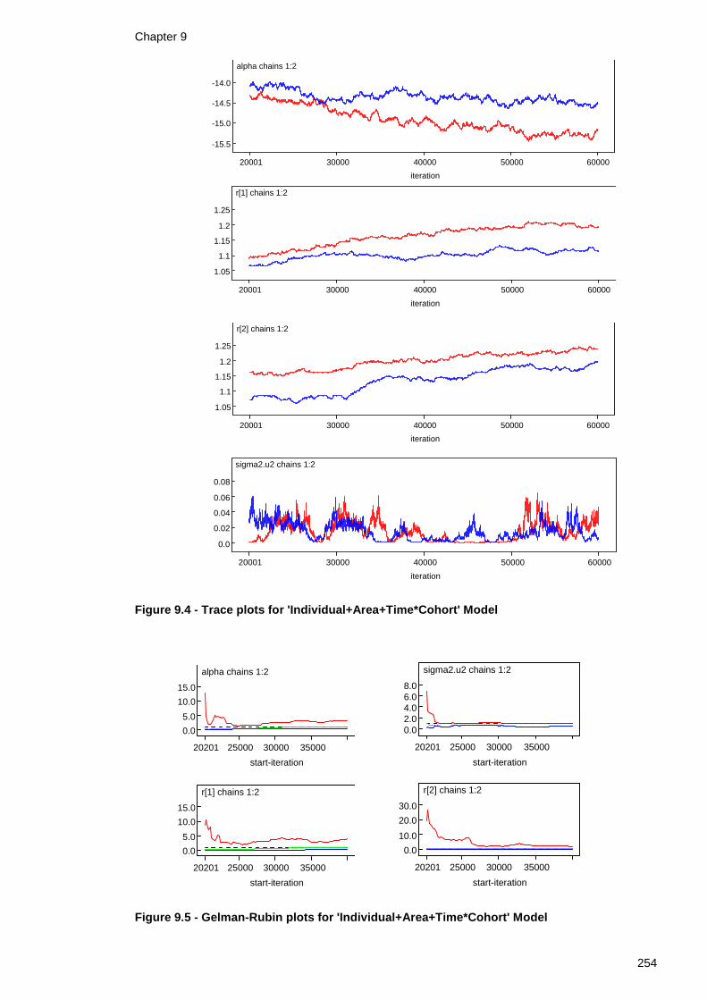
Chapter 9
254
alpha chains 1:2
iteration
20001 30000 40000 50000 60000
-15.5
-15.0
-14.5
-14.0
r[1] chains 1:2
iteration
20001 30000 40000 50000 60000
1.05
1.1
1.15
1.2
1.25
r[2] chains 1:2
iteration
20001 30000 40000 50000 60000
1.05
1.1
1.15
1.2
1.25
sigma2.u2 chains 1:2
iteration
20001 30000 40000 50000 60000
0.0
0.02
0.04
0.06
0.08
Figure 9.4 - Trace plots for 'Individual+Area+Time* Cohort' Model
alpha chains 1:2
start-iteration
20201 25000 30000 35000
0.0
5.0
10.0
15.0
sigma2.u2 chains 1:2
start-iteration
20201 25000 30000 35000
0.0 2.0 4.0 6.0 8.0
r[1] chains 1:2
start-iteration
20201 25000 30000 35000
0.0
5.0
10.0
15.0
r[2] chains 1:2
start-iteration
20201 25000 30000 35000
0.0
10.0
20.0
30.0
Figure 9.5 - Gelman-Rubin plots for 'Individual+Are a+Time*Cohort' Model

Chapter 9
255
Table 9.12 - MC error as a percentage of posterior standard deviation Individual+Area Individual+Area+Time*Cohort
MCE as % of SD MCE as % of SD
α
β1
β2 β3 β4 β5 β6 β7 β8 β9 β10 β11 β12 β13 β14 β15
r r1 (cohort1972) r2 (cohort1977)
σu2
6.0
4.8 5.5 5.4 5.2 4.9 5.0 4.9 5.3 4.1 4.7 5.0 4.9 4.6 4.1 4.2
6.0
5.7
5.0
3.8 4.6 4.6 4.3 4.0 4.0 3.9 4.1 3.1 3.5 5.0 3.9 3.5 3.1 3.2
5.0 5.0
4.8
For a burn-in period of 10000 iterations followed by a further 20000 iterations,
CPU time for the ‘Individual+Area’ frailty model was 251 064s; however, in real
time it was approximately 3.5 days. From comparing parameter estimates for
this model in Table 9.11 to those presented in Tables 9.7 and 9.10, obtained
using the discrete-time models and grouping according to covariates method
respectively, it can be seen that parameter estimates and standard errors for
the higher-level variation and all regression parameters apart from ‘cohort’ were
very similar. However, the parameter estimate for ‘cohort’ obtained from fitting
the Bayesian frailty model (=0.229) was larger than when discrete-time models
were fitted to the dataset before aggregation (=0.087) and after aggregation
according to covariates (=0.086). There are a few possible reasons that could
explain this difference. Firstly, from observing the trace plot in Figure 9.2 for
this parameter (β11), it can be seen that a bigger burn-in period might have been
required as the chains were not mixing perfectly by the end of the allotted burn-
in period (10000 iterations). The Gelman-Rubin plot for this same parameter
(Figure 9.3) indicated that a burn-in period of 12500 iterations may have been
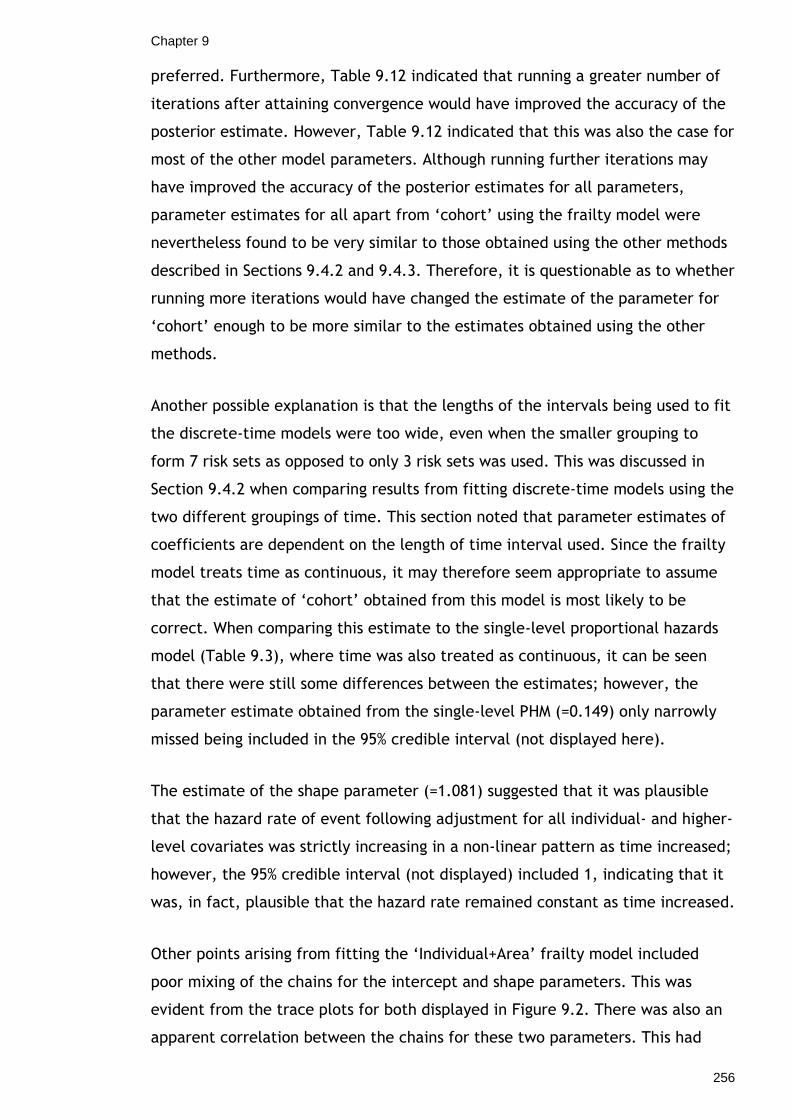
Chapter 9
256
preferred. Furthermore, Table 9.12 indicated that running a greater number of
iterations after attaining convergence would have improved the accuracy of the
posterior estimate. However, Table 9.12 indicated that this was also the case for
most of the other model parameters. Although running further iterations may
have improved the accuracy of the posterior estimates for all parameters,
parameter estimates for all apart from ‘cohort’ using the frailty model were
nevertheless found to be very similar to those obtained using the other methods
described in Sections 9.4.2 and 9.4.3. Therefore, it is questionable as to whether
running more iterations would have changed the estimate of the parameter for
‘cohort’ enough to be more similar to the estimates obtained using the other
methods.
Another possible explanation is that the lengths of the intervals being used to fit
the discrete-time models were too wide, even when the smaller grouping to
form 7 risk sets as opposed to only 3 risk sets was used. This was discussed in
Section 9.4.2 when comparing results from fitting discrete-time models using the
two different groupings of time. This section noted that parameter estimates of
coefficients are dependent on the length of time interval used. Since the frailty
model treats time as continuous, it may therefore seem appropriate to assume
that the estimate of ‘cohort’ obtained from this model is most likely to be
correct. When comparing this estimate to the single-level proportional hazards
model (Table 9.3), where time was also treated as continuous, it can be seen
that there were still some differences between the estimates; however, the
parameter estimate obtained from the single-level PHM (=0.149) only narrowly
missed being included in the 95% credible interval (not displayed here).
The estimate of the shape parameter (=1.081) suggested that it was plausible
that the hazard rate of event following adjustment for all individual- and higher-
level covariates was strictly increasing in a non-linear pattern as time increased;
however, the 95% credible interval (not displayed) included 1, indicating that it
was, in fact, plausible that the hazard rate remained constant as time increased.
Other points arising from fitting the ‘Individual+Area’ frailty model included
poor mixing of the chains for the intercept and shape parameters. This was
evident from the trace plots for both displayed in Figure 9.2. There was also an
apparent correlation between the chains for these two parameters. This had

Chapter 9
257
been a cause for concern when fitting the frailty model to the Scottish dataset.
Section 8.3.4 considered a re-parameterised version of the Weibull model which
could be fitted as a possible way of eliminating this correlation. Finally, the
trace plot for the higher-level variance in Figure 9.2 indicated that the Gibbs
sampler was tending to get trapped near zero. This resulted in slow convergence
for the parameter. This was another problem to have been observed when fitting
the frailty model to the Scottish dataset. A parameter expansion technique
aiming to speed up convergence was suggested in Section 8.3.5. The re-
parameterised Weibull model with variance expansion of Section 8.3.5 was fitted
to the Swedish dataset. Results are displayed in Table 9.13. Note that, due to
time constraints, this technique was only considered for the model containing
additive effects only (i.e. without the two-way interaction between ‘time’ and
‘cohort’). Trace plots and Gelman-Rubin plots for the intercept, shape
parameter of the Weibull distribution, higher-level variance and the regression
parameters for ‘cohort’ are given in Figures 9.6 and 9.7 respectively. Note that
plots for other regression parameters in the model are not displayed here.
To fit a two-way interaction between ‘time’ and ‘cohort’, the shape parameter
of the Weibull distribution was defined separately for each cohort. This allowed
the hazard to assume different shapes for each birth cohort year. The WinBUGS
code used to fit this model is given in Appendix 9. The model was run for a burn-
in period of 20000 iterations followed by a further 40000 iterations. CPU time
was 486 183 seconds. Parameter estimates for this model were compared with
those in Tables 9.7 and 9.10 for the same model. It can be observed that
estimates of all main effects (excluding ‘cohort’) and the higher level variance
were similar across the three tables (Tables 9.7, 9.10 and 9.11). The estimates
of the main effects and higher-level variance for the ‘Individual+Area’ and
‘Individual+Area+Time*Cohort’ obtained from fitting the Weibull model (Table
9.11) can also be compared. Table 9.12 indicated that the posterior estimates
for the ‘Individual+Area+Time*Cohort’ were more accurate than the
‘Individual+Area’ model, as the Monte Carlo error (MCE) for each parameter was
5% or less of the sample standard deviation. This was not the case for all
parameters in the ‘Individual+Area’ model. The improvements in the accuracy of
the results were most likely a consequence of running a further number of
iterations following the burn-in period.

Chapter 9
258
The trace plots for the regression parameters (excluding ‘cohort’) in Figure 9.4
indicated that the burn-in period of 20000 iterations was sufficient for attaining
convergence since the multiple chains in each plot were mixing well and were
stable around the mean value. However, it can also be observed that the
multiple chains for the intercept and shape parameters were not mixing well,
and there was evidence of correlation in the chains for these two parameters.
Furthermore, the trace plot for the higher-level variance indicated that the
Gibbs sampler was prone to getting trapped near zero. The re-parameterised
Weibull model with variance expansion may have been required to resolve these
problems.
Of most interest, however, are the estimates of the shape parameters defined
for each birth cohort year. Results in Table 9.11 indicated that the hazard
function for those in the 1977 cohort (r2 = 1.166) is increasing more steeply than
for those in the 1972 birth cohort (r1 = 1.132), thus confirming an interaction
between ‘time’ and birth cohort year. It should be noted, however, that there is
quite a lot of overlap in the 95% credible intervals (not displayed here) for r1 and
r2.

Chapter 9
259
Table 9.13 - Results from fitting re-parameterised Weibull model with variance expansion to the Swedish dataset Individual+Area
Estimate (s.e.) Fixed
Intercept (α) -15.44 (0.225)
Sex Male Female (β1)
0.000 0.490 (0.034)
Father Soc. Class 1980 Employers etc Non-manual (β2) Manual (β3) Unclassifiable (β4)
0.000 -0.132 (0.072) 0.133 (0.067) 0.527 (0.073)
Hhold Income Quintile Quintile 1 Quintile 2 (β5) Quintile 3 (β6) Quintile 4 (β7) Quintile 5 (β8) Missing (β9)
0.000 -0.150 (0.056) -0.176 (0.059) -0.112 (0.065) -0.299 (0.067) 0.451 (0.070)
Housing Tenure Owner Occupied Rented (β10)
0.000 0.480 (0.040)
Birth Cohort 1972 1977 (β11)
0.000 0.267 (0.035)
Economic Region Metropolitan Larger Regional (β12) Smaller Regional (β13) Private Enterprise(β14) Public Sector (β15)
0.000 -0.082 (0.043) -0.124 (0.060) 0.142 (0.095) -0.045 (0.136)
Shape (r) 1.228 (0.026)
Random Parish Variation(σu
2) 0.012 (0.010)

Chapter 9
260
alpha chains 1:2
iteration
15001 20000 30000 40000 50000
-16.5
-16.0
-15.5
-15.0
-14.5
r chains 1:2
iteration
15001 20000 30000 40000 50000
1.15
1.2
1.25
1.3
1.35
beta[11] chains 1:2
iteration
15001 20000 30000 40000 50000
0.1
0.2
0.3
0.4
sigma2.u2 chains 1:2
iteration
15001 20000 30000 40000 50000
0.0
0.02
0.04
0.06
Figure 9.6 - Trace plots for re-parameterised Weibu ll model with variance expansion

Chapter 9
261
alpha chains 1:2
start-iteration
15201 20000 25000 30000
0.0 2.0 4.0 6.0 8.0
r chains 1:2
start-iteration
15201 20000 25000 30000
0.0 2.5 5.0 7.5 10.0
beta[11] chains 1:2
start-iteration
15201 20000 25000 30000
0.0
1.0
2.0
3.0
sigma2.u2 chains 1:2
start-iteration
15201 20000 25000 30000
0.0 0.5 1.0 1.5 2.0
Figure 9.7 - Gelman-Rubin plots for re-parameterise d Weibull model with variance expansion
The re-parameterised Weibull model with parameter expansion was run for a
burn-in period of 15000 iterations, with a further 40000 iterations run after the
burn-in period to obtain posterior estimates. CPU time was 593 835 seconds, i.e.
approximately seven days. Recall that this model was fitted in order to try and
eliminate the correlation between the chains for the intercept, alpha and the
shape parameter, r. Therefore, parameter estimates, trace plots and Gelman-
Rubin plots should be compared to Table 9.11 and Figures 9.2 and 9.3
respectively.
To determine whether using a re-parameterised version of the Weibull model has
eliminated the correlation between the intercept and the shape parameter, it
was of most interest to observe the trace plots for these parameters (Figure 9.6)
and compare them to the trace plots for the same parameters in Figure 9.2. It
can be seen that the multiple chains for both the intercept and the shape
parameter were mixing better in Figure 9.6 following the re-parameterisation
than in Figure 9.2. There was still some evidence of correlation in the multiple
chains; however, it had been greatly reduced following the re-parameterisation.
This would support the use of the re-parameterised model.
It was also of most interest to compare the trace plot for the higher-level
variance, σu2, in Figure 9.6 to that in Figure 9.2 in order to determine whether
using a parameter expansion technique had been successful in preventing the
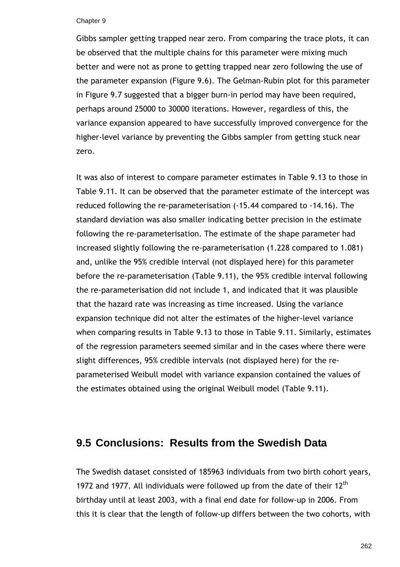
Chapter 9
262
Gibbs sampler getting trapped near zero. From comparing the trace plots, it can
be observed that the multiple chains for this parameter were mixing much
better and were not as prone to getting trapped near zero following the use of
the parameter expansion (Figure 9.6). The Gelman-Rubin plot for this parameter
in Figure 9.7 suggested that a bigger burn-in period may have been required,
perhaps around 25000 to 30000 iterations. However, regardless of this, the
variance expansion appeared to have successfully improved convergence for the
higher-level variance by preventing the Gibbs sampler from getting stuck near
zero.
It was also of interest to compare parameter estimates in Table 9.13 to those in
Table 9.11. It can be observed that the parameter estimate of the intercept was
reduced following the re-parameterisation (-15.44 compared to -14.16). The
standard deviation was also smaller indicating better precision in the estimate
following the re-parameterisation. The estimate of the shape parameter had
increased slightly following the re-parameterisation (1.228 compared to 1.081)
and, unlike the 95% credible interval (not displayed here) for this parameter
before the re-parameterisation (Table 9.11), the 95% credible interval following
the re-parameterisation did not include 1, and indicated that it was plausible
that the hazard rate was increasing as time increased. Using the variance
expansion technique did not alter the estimates of the higher-level variance
when comparing results in Table 9.13 to those in Table 9.11. Similarly, estimates
of the regression parameters seemed similar and in the cases where there were
slight differences, 95% credible intervals (not displayed here) for the re-
parameterised Weibull model with variance expansion contained the values of
the estimates obtained using the original Weibull model (Table 9.11).
9.5 Conclusions: Results from the Swedish Data
The Swedish dataset consisted of 185963 individuals from two birth cohort years,
1972 and 1977. All individuals were followed up from the date of their 12th
birthday until at least 2003, with a final end date for follow-up in 2006. From
this it is clear that the length of follow-up differs between the two cohorts, with
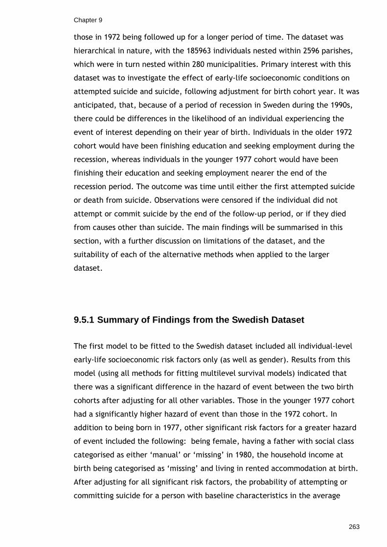
Chapter 9
263
those in 1972 being followed up for a longer period of time. The dataset was
hierarchical in nature, with the 185963 individuals nested within 2596 parishes,
which were in turn nested within 280 municipalities. Primary interest with this
dataset was to investigate the effect of early-life socioeconomic conditions on
attempted suicide and suicide, following adjustment for birth cohort year. It was
anticipated, that, because of a period of recession in Sweden during the 1990s,
there could be differences in the likelihood of an individual experiencing the
event of interest depending on their year of birth. Individuals in the older 1972
cohort would have been finishing education and seeking employment during the
recession, whereas individuals in the younger 1977 cohort would have been
finishing their education and seeking employment nearer the end of the
recession period. The outcome was time until either the first attempted suicide
or death from suicide. Observations were censored if the individual did not
attempt or commit suicide by the end of the follow-up period, or if they died
from causes other than suicide. The main findings will be summarised in this
section, with a further discussion on limitations of the dataset, and the
suitability of each of the alternative methods when applied to the larger
dataset.
9.5.1 Summary of Findings from the Swedish Dataset
The first model to be fitted to the Swedish dataset included all individual-level
early-life socioeconomic risk factors only (as well as gender). Results from this
model (using all methods for fitting multilevel survival models) indicated that
there was a significant difference in the hazard of event between the two birth
cohorts after adjusting for all other variables. Those in the younger 1977 cohort
had a significantly higher hazard of event than those in the 1972 cohort. In
addition to being born in 1977, other significant risk factors for a greater hazard
of event included the following: being female, having a father with social class
categorised as either ‘manual’ or ‘missing’ in 1980, the household income at
birth being categorised as ‘missing’ and living in rented accommodation at birth.
After adjusting for all significant risk factors, the probability of attempting or
committing suicide for a person with baseline characteristics in the average

Chapter 9
264
parish within municipality was small (≈ 0.00158). All variation was at parish level
(i.e. there was no variation in the hazard of event between municipalities), and
was bordering on significance. Although the between-parish variation was fairly
small (≈ 0.022), it was large in comparison to the hazard of event in the average
parish within municipality.
A contextual-level variable was then added to the model containing all
individual-level variables. This variable was an indicator of the type of economic
region. Although there were no significant differences when comparing each
level of region to the baseline, i.e. metropolitan regions, adding this variable to
the model explained some more of the variation between parishes within
municipalities (≈ 23% of the variation). Whilst the effect of cohort on the hazard
of event was attenuated when adding economic region, there were still
significant differences between the two cohorts after adjusting for the other
variables.
Two further models were fitted; one which included all individual- and higher-
level additive effects plus two-way interactions between cohort and each of the
other variables and another which included all additive effects and a two-way
interaction between time and cohort. It was of interest to fit the first model to
investigate if the effect of gender and each of the early-life socioeconomic risk
factors on the hazard of event differed between the two birth cohort years.
Generally, there was no strong indication that the effect of gender and the
socioeconomic variables on the hazard of event differed between cohort years;
however, there was a suggestion that living in smaller regional centres
(compared to metropolitan areas) significantly increased the hazard of event for
those born in 1977 compared to those born in 1972. There was also a weak
suggestion that the hazard of event was significantly higher for those born in
1977 compared to those born in 1972 when household income at birth was in the
third or fourth quintile (compared to quintile 1).
Finally, results from the model containing all additive effects plus a two-way
interaction between time and cohort suggested that as time increased, the
hazard of attempting or committing suicide differed between the two cohorts. It
could be observed that the hazard of event in the third and sixth risk sets
(compared to the first risk set) differed between the two cohorts, with those in

Chapter 9
265
the 1977 cohort having a significantly higher hazard of event at these times than
those in the 1972 cohort. An explanation of this result was given in Section
9.4.2.
9.5.2 Limitations of the Data
The main limitation of the Swedish dataset was the lack of information available
on reasons for missing data. Results showed that those categorised as
‘unclassifiable or missing’ for the variables ‘father’s social class in 1980’ and
‘household income at birth’ had the highest hazard of event compared to the
baseline categories. It would have been beneficial to know why these data had
been coded as ‘unclassifiable or missing’ in the first place, in order to determine
what it was about those categories that increased the hazard of event. One
possible explanation could have been unemployment. If an individual’s father
was unemployed in 1980 then it may not have been possible to assign one of the
other social class categories to this observation. Similarly, if there was no
household income at birth, then observations may again just have been coded as
missing. If this were the case, then it would suggest that individuals whose
parents were unemployed during early childhood years could be at greater risk
of attempting or committing suicide during their teenage years and in early
adulthood.
Another point concerning missing data was the way it was handled during
analyses. Although individuals with missing data for the ‘social class’ and
‘household income’ variables were coded as a separate category and included in
analysis as described above, some individuals also had missing data for the
‘housing tenure at birth’ and ‘economic region’ variables. Individuals with
missing data on either of these variables were excluded from analysis. As
discussed in Section 4.1.3, ignoring missing data can lead to loss of power or
biased estimates of associations. Since it is known that even a small proportion
of missing data can potentially bias results, it would have been preferable to
impute values for the missing data rather than exclude the cases; however, due
to time constraints on analyses, methods of missing value imputation were not
employed. This would be a recommendation for further work with this dataset.

Chapter 9
266
9.6 Conclusions: Suitability of Methods
The primary aim of using the Swedish dataset was to investigate which of the
alternative methods described in Chapter 7 performed well when fitted to a
much larger dataset. The Swedish dataset was larger than the Scottish ‘training’
dataset, in terms of both the number of individuals and the length of follow-up.
As with the Scottish dataset, there was a high percentage of censored
observations in the Swedish dataset (approximately 98%). This section
summarises how well each of the methods being considered as an alternative to
fitting multilevel continuous-time proportional hazards models in MLwiN
performed when fitted to the large Swedish dataset.
Since the Swedish dataset was large to begin with (containing 185 963
individuals), it was anticipated that treating time as a continuous variable would
not be a plausible option. As discussed throughout this thesis, fitting multilevel
continuous-time models in MLwiN requires the creation of a person-period
dataset so that each individual’s record is replicated for each time point until
the individual experiences the event of interest or is censored. When an event is
rare, this implies that most individuals will have a line of data for all time
points, which poses a problem if the period of follow-up is long. The Swedish
dataset was much too large to allow creation of the person-period dataset in
MLwiN when time was being treated as a continuous variable (i.e. measured in
days). Thus, alternative methods had to be adopted in order to fit multilevel
survival models to this dataset.
The first alternative method to be considered involved defining different risk
sets, so that time was divided into discrete intervals instead of being treated as
continuous. Various groupings of time were considered for the Swedish dataset,
as displayed in Table 9.4. It was of interest to investigate how narrow intervals
could be before estimating models in MLwiN became problematic. Recall that
the shorter the length of the time interval the more risk sets there are, thus
resulting in a larger person-period dataset. Similarly, it was also of interest to
determine the smallest number of risk sets permitted without losing precision in
the estimates by having long time intervals. The smallest person-period dataset
which could successfully fit multilevel discrete-time survival models in MLwiN

Chapter 9
267
without losing precision in estimates contained just over 1.2 million observations
within individuals. Results from fitting multilevel discrete-time models were
presented and discussed in Section 9.4.2. Results suggested that various
groupings of time should be considered when defining discrete time intervals in
order to ensure that no information is being lost by having wider intervals and
thus, fewer risk sets. Models should be fitted to the person-period dataset
obtained from using the grouping of time that leads to the smallest number of
risk sets (and hence the smallest person-period dataset) without changing the
parameter estimates of coefficients. Alternatively an estimator adjusting for
time aggregation bias, or the complementary log-log link function as opposed to
the logistic, should be used.
The second alternative method to be considered involved aggregating the data
of individuals within the same higher-level units, who had the same values for
covariates included in a particular model. This implied that just one line of data
represented all such individuals. Aggregating the data in this way can lead to a
reduction in the size of the expanded dataset. Although it should be possible to
fit both multilevel continuous-time and discrete-time survival models to the
aggregated dataset, because the person-period dataset could not be created in
MLwiN for the Swedish data when time was continuous, only discrete-time
models could be fitted. This is because the aggregated dataset has to be
constructed from the person-period dataset.
This method works best when there are a large number of individuals nested
within each of the higher-level units, when the number of covariates to be
grouped on is small and when covariates are categorical variables. Because all of
these criteria were satisfied when aggregating the Swedish dataset, grouping the
data in this way led to a large percentage reduction, over 50%, in the size of the
person-period dataset before aggregation.
The final alternative method to be considered involved fitting Bayesian survival
‘frailty’ models in WinBUGS and using MCMC methods of estimation. In WinBUGS,
an additive frailty model is adopted and a Weibull distribution is assumed for the
survivor function. There are a number of reasons why this approach may be
favoured over the others. Firstly, the Weibull model does not require the
creation of a person-period dataset, and therefore there are no concerns over
Chapter 9
268
the dataset becoming too large to work with. Recall that the Swedish dataset
contained 185963 individuals, or 185449 individuals after excluding those with
missing data. Secondly, time is treated as a continuous variable in the Weibull
model, and thus there is no time aggregation bias implying that parameter
estimates may be more accurate than when using discrete-time models. The
Weibull model fitted to the Swedish dataset using MCMC estimation produced
results which were consistent with those obtained from fitting the other
alternative methods in MLwiN. However, as with the Scottish dataset, there was
the problem of slow convergence for some parameters. A re-parameterised
version of the Weibull model which incorporated a parameter expansion was
adopted in an attempt to overcome these problems.
This section has detailed how well the three alternative methods performed
when fitted to a large dataset. Recommendations for which of the three
methods may be the most suitable, depending on, for example, the type of data,
the research questions etc, are given in Chapter 10.

269
10 Discussion
10.1 Introduction
Event history models, or survival models, as they are more commonly referred to
in medical applications, are applied when the outcome is a measure of duration.
Therefore, they are important in the field of public health where it is often of
interest to measure time until a particular pre-defined event occurs, such as
death from some disease.
It is widely acknowledged that, for many outcomes, the health of individuals
varies across geographical locations. Since this can also be true of event times,
it is important that such survival data are analysed using multilevel survival
models. These account for the dependence of event times nested within the
same geographical location. Although multilevel survival models have been
developed, computational requirements mean that their use is limited for large
datasets. As discussed in Section 1.3, this poses a problem for those working in
the field of public health since datasets for monitoring and measuring public
health outcomes are typically large. Additionally, public health survival datasets
may contain a large proportion of censored observations, because either the
event of interest is rare or the period of follow-up is long. This poses a further
problem since having many censored observations can also be troublesome when
estimating multilevel survival models.
To recap from Section 1.3, the purpose of this thesis was to investigate ways in
which multilevel survival models could be developed to model large datasets
with a large proportion of censored observations. It is hoped that this will make
them more accessible to those working in public health. Two datasets were
employed for this purpose. The first was a moderately-sized Scottish dataset
which was used as a training dataset to explore the limitations of existing
software packages for fitting multilevel survival models, and then to develop
alternative methods. Once alternative methods had been developed using this
dataset, they were then applied to a second much larger dataset from Sweden
to test how effective these alternative methods were when fitted to a larger

Chapter 10
270
dataset. Section 10.2 provides a summary of methodological findings from the
Scottish training dataset and the larger Swedish dataset.
10.2 Summary of Methodological Findings
A software package specially designed for fitting multilevel models to
hierarchical data is MLwiN. Although fitting multilevel survival models is not a
standard feature of MLwiN, macros are available for fitting two of the most
commonly used survival models for modelling the effect of covariates on an
outcome of duration. These are the proportional hazards model and the
accelerated lifetime model. Because of the high proportion of censoring in the
Scottish training dataset, a multilevel accelerated lifetime model could not be
fitted for reasons discussed in Section 5.4.1. This meant that only the multilevel
continuous-time proportional hazards model could be estimated in MLwiN for
this dataset. Section 5.3.3.1 demonstrated how a proportional hazards model
can be fitted via a Poisson model, which is the method adopted in MLwiN. This
section also demonstrated how the person-period dataset required to fit the
Poisson model could be created. This required that each individual’s record be
replicated as many times as the observed number of time points until either the
event of interest or censoring occurred. As time is being treated as a continuous
variable when fitting the Poisson model, creating the person-period dataset can
lead to a vast expansion in the size of the original dataset, especially if the
period of follow-up is long. Additionally, if the event of interest is rare, then the
majority of individuals in the dataset would have a record of data corresponding
to every continuous time point at which an event occurred. With the Scottish
dataset, which originally consisted of 15305 individuals, creation of the person-
period dataset led to an expanded dataset containing approximately 1.9 million
observations within individuals.
MLwiN was able to cope with fitting the multilevel Poisson model to this size of
dataset, the only problem being that the first-order PQL estimation procedure
had to be used instead of the preferred second-order PQL procedure. However,
since the Scottish dataset was only moderately-sized in the realm of public

Chapter 10
271
health datasets, it was necessary to investigate other methods which could be
used as an alternative to multilevel continuous-time models when datasets are
much larger. Indeed, Section 9.4.1 revealed that the use of multilevel
continuous-time models in MLwiN for the large Swedish dataset, which consisted
of 185963 individuals, was impossible. This was because the dataset was too
large to be expanded in order to create the person-period dataset to which the
Poisson models are then fitted.
Three alternative methods were discussed in Chapter 7 and were applied to the
Scottish training dataset, with results displayed in Chapter 8. Two of the
alternative methods were applied in MLwiN; however, the third method involved
fitting Bayesian multilevel survival (frailty) models in WinBUGS and using MCMC
methods of estimation. The three alternative methods were then fitted to the
Swedish dataset to test their suitability for modelling a much larger dataset
(Chapter 9). The performance of these three methods when fitted to the both
datasets is now considered.
The first alternative method, as discussed in Section 7.2, involved defining
different risk sets and fitting discrete-time hazard models. Instead of treating
time as a continuous variable, thus having to define a risk set for each time at
which an event occurred, this method involved dividing time into discrete time
intervals, either of equal or varying length. Dividing time like this led to a
reduction in the number of risk sets, and thus a reduction in the size of the
person-period dataset. On creation of the person-period dataset using this new
discrete-grouping of time, standard methods for fitting multilevel models to
discrete response data, such as logistic regression, could be employed. Indeed,
it was the logistic link function that was used to fit the multilevel discrete-time
model to the Scottish training dataset. Dividing time into discrete-time intervals,
either when intervals were divided into equal lengths or varying lengths,
constructed according to when events occurred, led to a vast reduction in the
size of the continuous-time person-period dataset. The percentage reductions in
the continuous-time person-period dataset were approximately 94% and 97%
respectively when intervals were of equal and varying lengths. The discrete-time
modelling approach also worked well when fitted to the large Swedish dataset,
although various attempts at dividing up time had to be considered in order to
find the smallest number of discrete-time intervals permitted, and hence the

Chapter 10
272
smallest number of risk sets, without influencing estimates of coefficients. It
was of interest to have fewer risk sets since this implies a smaller person-period
dataset.
The second alternative method, as discussed in Section 7.3, was termed
‘grouping according to covariates’, and involved aggregating the data of
individuals within the same higher-level units who had the same values for
covariates included in a particular model so that one line of data was used to
represent all such individuals. The concept behind this method is that all
individuals within the same geographical location with the same values for
covariates included in a particular model are at risk of experiencing the event of
interest at the same time. As a result, all of these individuals can be
represented by one line of data. Aggregating the data in this way can lead to a
reduction in the size of the expanded dataset. The multilevel continuous-time
and discrete-time survival models employed by MLwiN can be adapted to model
the aggregated dataset. This was covered in Sections 7.3.2 and 7.3.3. Both
continuous-time and discrete-time models were fitted to the aggregated Scottish
dataset. When time was treated as continuous, implying a risk set for each
distinct event time, aggregating the dataset reduced the size of the continuous-
time person-period dataset (before aggregation) by between 4% and 84%. This
depended upon how many covariates were used for the grouping. Time was then
treated as discrete and, although the widths of the intervals could be equal or
varying, the most successful percentage reduction in the continuous-time
Scottish person-period dataset occurred when intervals were varying in length,
leading to a reduction of between 97% and 99.5%. Again, this percentage
depended upon how many covariates were used for the grouping. This method
also worked well when fitted to the large Swedish dataset; however, because
the aggregated dataset must be created using the person-period dataset, only
discrete-time models could be fitted to the Swedish dataset since it was too
large to create the person-period dataset when time was continuous. When time
was discrete, grouping according to all individual- and higher-level covariates
led to a reduction of over 50% in the discrete-time person-period dataset before
aggregation.
The final alternative method to be considered involved fitting Bayesian survival
‘frailty’ models in WinBUGS and using the MCMC method of estimation, as

Chapter 10
273
discussed in Section 7.4. In WinBUGS, an additive frailty model is adopted and a
Weibull distribution is assumed for the survivor function. It was shown that the
regression parameter estimates obtained from the Weibull model could be
interpreted as hazard ratios; hence they were comparable with those obtained
from fitting the continuous-time Poisson model. However, when fitting frailty
models to the Scottish dataset, although parameter estimates of fixed and
random effects obtained from the Weibull model were very similar to those
obtained using the Poisson model in MLwiN, trace plots revealed some poor
mixing of Markov chains for some parameters, as well as the Gibbs sampler
tending to get trapped near zero for the random-effects variance. It was
hypothesised that the high percentage of censored observations could be the
root of the problems, with the Weibull model failing to provide a good fit in the
presence of many censored observations. However, a simulation study revealed
that the high percentage of censoring only slightly affected parameter
estimates, and could not explain the poor mixing of Markov chains for some
parameters. Therefore, it was necessary to consider, instead, a re-
parameterised version of the Weibull model, which also included a parameter
expansion to help speed up convergence for the random-effects variance. Similar
problems were encountered when fitting the Bayesian frailty model to the
Swedish dataset; therefore the re-parameterised Weibull model with the
parameter expansion was considered for this dataset also. As with the Scottish
dataset, using the re-parameterised version of the Weibull model successfully
improved the poor mixing and reduced the correlation in the chains for the
intercept and the shape parameter of the Weibull distribution. Furthermore,
using the variance expansion technique appeared to be more effective at
speeding up convergence for the higher-level variance when fitted to the
Swedish dataset than it had been when used in the Weibull model fitted to the
Scottish dataset.
There were further points for consideration when the Weibull model was fitted
to the Swedish dataset. Unlike the Scottish dataset, for which the proportional
hazards assumption had been reasonable, there was evidence of time-varying
covariates in the Swedish dataset. When fitting either the continuous-time or
discrete-time hazard model in MLwiN, time-varying covariates are easily
incorporated by including an interaction between the time-dependent variable

Chapter 10
274
and the baseline hazard function. However, in the Weibull model this could
prove to be problematic as the baseline hazard function is restricted to be
monotonically increasing, decreasing or constant [263]. A possible solution would
be to use the piecewise Weibull model. The piecewise Weibull model allows the
Weibull baseline hazard function to change at unknown change points [263].
Tarrés et al. [264] and Casellas [263] demonstrated how the inclusion of time-
varying covariates converted the Weibull hazard function into a piecewise
Weibull (or Weibull time-dependent) hazard function. They showed how a
different slope is defined for each period of time, where the cut-point (or
change point) of the time period can be established either using a spline
regression [264] or treating them as unknown parameters in the model to be
estimated [263]. The differing slopes represent the differing hazards in each
time period.
10.3 Conclusions
This thesis has considered a number of ways in which multilevel survival models
can be fitted to large datasets with a high percentage of censored observations.
Based on the results from each of these methods, as summarised in Section 10.2,
this section will provide recommendations on the effectiveness of each method
by considering the advantages and disadvantages of each.
Fitting a Poisson model in MLwiN may seem like an appealing option since, after
creation of a person-period dataset, the (exponentials of) regression parameters
in the Poisson model provide identical estimates of hazard ratios obtained from
proportional hazards models. In addition, there is no time-aggregation bias when
time is treated as continuous, since each distinct event time corresponds to a
separate risk set. However, although this method is effective for small to
moderately sized datasets, this thesis has shown that it fails when fitted to large
datasets. As a result, fitting multilevel Poisson models in MLwiN would not be
recommended to those working in the field of public health, where datasets
typically tend to be large in size, unless they are sure that the dataset in
question is small enough to be expanded for creation of the person-period
Chapter 10
275
dataset. An alternative continuous-time model which can be implemented in
MLwiN is the accelerated lifetime model. This approach may be more favourable
than the Poisson modelling approach as no data expansion is required to fit the
accelerated lifetime model. However, it is recommended that this model is not
used if at least half of the observations in the dataset are censored. This is
because estimation procedures used in MLwiN to estimate non-linear models
(quasi-likelihood under IGLS) are prone to breaking down for this model when
there is a high proportion of censored observations. As a result, the accelerated
lifetime model may also not be recommendable to those working in public
health, unless the outcome of interest and the length of follow-up time are such
that no more than fifty percent of observations in a dataset are censored.
Fitting discrete-time models in MLwiN can be a useful alternative to fitting
continuous-time models. Because risk sets correspond to discrete-time intervals
instead of each distinct event time, the size of the person-period dataset also
required to fit these models can be greatly reduced. On creation of the person-
period dataset, fitting discrete-time models in MLwiN is straightforward since
standard approaches to modelling discrete response data, such as logistic
regression, may be used. Other advantages of the discrete-time approach
include that it can easily incorporate tied observations and time-varying
covariates. There are, however, some potential problems with this method
which must be considered before using it for data analysis.
One potential problem with using the discrete-time model is that estimates of
coefficients depend on the length of time interval when the logistic link function
is used; therefore, estimates from this model may not be completely identical to
those obtained from fitting a continuous-time model. However, if the width of
each discrete-time interval is small enough, then the logistic model converges to
the proportional hazards model, meaning estimates of coefficients will be more
similar. Therefore, when using this method, it is necessary to experiment with
the widths of the discrete-time intervals in order to find a trade-off between
having the smallest number of discrete-time intervals, and hence the smallest
number of risk sets, so that the size of the person-period dataset is as small as
possible without influencing coefficient estimates. If using the discrete-time
approach, it may be advisable to, first, run a single-level proportional hazards
model to get a rough idea of parameter estimates. This will determine whether

Chapter 10
276
estimates obtained using the discrete-time approach are being influenced by the
length of the time intervals. Alternatively, an adjustment for time-bias could be
included, or the complementary log-log link could be used as opposed to the
logistic. Use of the complementary log-log link was not considered here because
of time constraints, and also because of the computational convenience and
easier interpretation when the logistic function is used, thus making its use more
desirable.
When fitting multilevel survival models in MLwiN, either using the continuous-
time Poisson modelling approach or the discrete-time modelling approach, the
size of the person-period dataset required for both methods can be reduced
further by grouping according to covariates. However, as discussed throughout
this thesis, this method is not the easiest to implement for a number of reasons.
Firstly, the aggregated dataset has to be re-created each time the covariates in
a particular model change. As a result, this method would not be recommended
for model selection. Secondly, the effectiveness of this method at reducing the
size of the person-period dataset depends largely on the number of covariates to
be grouped on and the number of individuals within each higher-level unit. If on
average there are a large number of individuals clustered within each higher-
level unit, then there is a greater chance that there will be more individuals
within that higher-level unit sharing the same values for the covariates to be
grouped on. This would lead to a greater reduction in the person-period dataset
and vice versa. Ultimately, however, it is clear that, regardless of the number of
individuals per higher-level unit, the number of individuals with identical
covariates becomes smaller as the number of covariates to be grouped on
increases. Further to this, if risk factors are measured on a continuous scale, the
number of individuals sharing exact values for continuous risk factors will
decrease as the number of continuous risk factors to be grouped on increases. It
should be noted also that, because the aggregated dataset must be constructed
from the person-period dataset, only discrete-time models can be used if a
dataset is very large for reasons discussed earlier in this section.
Although there are many issues which must be considered before adopting the
grouping according to covariates method, it can be very effective in reducing
the size of the person-period dataset, as demonstrated with both the Scottish
and Swedish datasets. Once a final model has been selected, provided that there

Chapter 10
277
are, on average, a large number of individuals per higher-level unit, not too
many covariates in the final model, and that the majority of covariates are
categorical, this method can lead to a vast reduction in the size of the person-
period dataset before aggregation. As a result more preferable methods of
estimation in MLwiN, such as second-order PQL, may become available due to
the reduction in the size of the person-period dataset.
An entirely different approach which may be adopted is to fit Bayesian survival
(frailty) models and use MCMC methods of estimation. Such models can be easily
implemented in WinBUGS, a package designed specially to make practical MCMC
methods available to applied statisticians. There are a number of reasons why a
Bayesian approach may be preferred over a traditional frequentist approach.
Firstly, the Bayesian approach allows any prior knowledge about parameters to
be incorporated into analysis. This may be useful in the field of public health if a
particular research problem has been considered before in previous studies
meaning that prior information is available on the parameters of interest.
Secondly, with the recent advances in computing technology, Bayesian inference
using MCMC allows more complex models to be fitted straightforwardly.
More specifically, however, there are also reasons why fitting multilevel survival
models in WinBUGS may be preferred to MLwiN. Unlike the approaches adopted
in MLwiN in this thesis, fitting frailty models in WinBUGS does not require
creation of a person-period dataset, and thus there is no issue of a dataset
becoming too large to work with following expansion. Also, time is treated as
continuous when fitting frailty models in WinBUGS implying that there are no
concerns over time-aggregation bias. Lastly, there is also much more flexibility
in the choice of frailty distribution in WinBUGS than in MLwiN. The frailty is the
exponential of the random effects and in MLwiN it is constrained to follow a log-
Normal distribution, whereas any distribution can be selected for this term in
WinBUGS.
Although fitting Bayesian survival models in WinBUGS may seem like a more
appealing approach than fitting these models in MLwiN, there are some
drawbacks to the Bayesian approach. Estimating models using MCMC can take
longer than estimating the same models using quasi-likelihood methods.
Although various techniques such as re-parameterisation and parameter

Chapter 10
278
expansion can be employed to speed up convergence with the aim of reducing
computing time, if quick estimation of models is required, this would not be the
best approach. This is especially a problem when the dataset in question is
large, and also if there are a lot of covariates in the model. However, if
computing time is not important, then this approach, due to its greater
flexibility, may be more favourable than the frequentist approaches.
This thesis has shown that there are a number of efficient methods which can be
used to model large, hierarchically-structured, survival datasets as an
alternative to continuous-time models. However, before selecting one of these
approaches, public health researchers should first consider what the main
objectives of the research are. If interest lies in quickly analysing a dataset to
determine associations between covariates and event times, then the discrete-
time approach in MLwiN may be desirable as models can be estimated quickly
and straightforwardly using, for example, logistic regression models fitted to a
person-period dataset. It may also be possible to reduce the size of the person-
period dataset by grouping according to covariates. The frailty modelling
approach in WinBUGS would not be favourable here as models take a long time
to run using MCMC when datasets are large. However, if computing time is not
an issue, then fitting frailty models in WinBUGS may be more desirable because
of the greater flexibility in using a Bayesian approach. Furthermore, parameter
estimates may be more accurate since time is treated as continuous, and thus
there are no concerns over time-aggregation bias.
10.4 Implications of the Findings
In the past, the use of multilevel survival models in the field of public health has
been limited because datasets used for measuring and monitoring public health
are typically large. Large datasets pose a problem when trying to fit commonly
used multilevel survival models such as the proportional hazards models, in
conventional multilevel software packages such as MLwiN. This thesis has
introduced alternative approaches which can be employed to make multilevel
survival models more accessible to those working in public health, and this

Chapter 10
279
section considers what the research in this thesis has contributed to the wider
literature.
In Chapter 5, forty papers fitting multilevel survival models to real datasets
were reviewed; not all were public health datasets. From these forty papers, ten
were selected as meeting the criteria for being classed as large datasets. To
meet these criteria, the datasets in question had to either consist of more than
15305 individuals and/or have a follow-up period of more than 9 years. These
conditions were defined as it had already been demonstrated using the Scottish
dataset that multilevel proportional hazards models, estimated via Poisson
models in MLwiN, could be fitted without any problems to datasets of this size.
Therefore, it was not of interest to consider datasets smaller than this. Of the
ten papers reviewed, the authors had considered various options to fit multilevel
survival models to their datasets. MLwiN was the most commonly used package,
with half of the papers using it to fit the models. Most authors using MLwiN
stratified analysis by breaking-up the datasets into smaller cohorts in order to
make the person-period dataset of a more manageable size for fitting
proportional hazards models. This thesis has introduced methods which do not
require the need to break up datasets in order to fit multilevel survival models.
Another of the papers that used MLwiN implemented the accelerated lifetime
model; however, as discussed throughout this thesis, the use of MLwiN to
estimate this model is not recommended if there is a high proportion of
censored observations. This can occur in public health if the event of interest is
rare. This thesis has considered models which can still be easily estimated, even
when the proportion of censored observations is high.
One of the reviewed papers was able to successfully implement the proportional
hazards model on a very large dataset using the R software package. This could
be yet another alternative way of fitting continuous-time models as opposed to
using MLwiN or WinBUGS; however, it was noted that R can only be used to fit
multilevel models when there is just one random effect. For many public health
datasets, there may be more than one higher level, as with the Swedish dataset
in this thesis; thus the use of R would not be suitable. This thesis has introduced
methods which can incorporate more than one random effect.

Chapter 10
280
Only one of the reviewed papers adopted a Bayesian approach to fitting
multilevel survival models. Authors fitted an additive frailty model in WinBUGS,
the same approach as taken in this thesis. This thesis aims to assist in increasing
the awareness of public health researchers to the possibility of using Bayesian
survival (frailty) models as an alternative to traditional frequentist approaches.
To summarise, this thesis has attempted to contribute to the wider literature by
introducing approaches for dealing with many of the problems posed by public
health datasets. For example, it has shown that multilevel survival models can
still be fitted when datasets are large, when there is a high percentage of
censored observations and when there is more than one higher level. It has also
highlighted the possibility of using a Bayesian approach instead of traditional
frequentist methods.
10.5 Limitations and Recommendations
This section will summarise the methodological limitations of this research and
recommend areas for further work based on these limitations. Limitations
concerning the datasets used in this thesis will not be considered here since this
has already been covered in Chapter 6 for the Scottish data and in Section 9.5.2
for the Swedish data.
10.5.1 Methodological Limitations and Recommendatio ns
For each of the four methods employed for fitting multilevel survival models in
this thesis, i.e. the Poisson, discrete-time and grouping according to covariates
modelling in MLwiN, and the frailty modelling approach in WinBUGS, Section
10.3 gave a detailed account of the advantages and disadvantages of each. The
disadvantages may be seen as limitations of using these methods. For example,
Section 10.3 discussed that, when fitting discrete-time models, it is advisable to
experiment with the widths of the discrete-time intervals in order to find a
trade-off between having the smallest number of discrete-time intervals, and

Chapter 10
281
hence the smallest number of risk sets so that the size of the person-period
dataset is as small as possible without influencing coefficient estimates. This
implies having to create a new person-period dataset for each different division
of time being considered, as well as having to run models using each different
division of time in order to compare estimates of coefficients from each.
Therefore, in practice, this method has the potential to be quite cumbersome.
For the grouping according to covariates approach, Section 10.3 discussed how
this method is most suitable when there are a large number of individuals nested
within each of the higher-level units, when the number of covariates to be
grouped on is small, and when covariates are categorical variables. These can be
a lot of conditions to satisfy, and therefore this method may not prove very
efficient in a lot of circumstances. This could be particularly true if using this
method for applications outside public health. In public health and
epidemiology, a lot of data on risk factors tends to be categorical; however, this
may not be the case in other fields of research.
The biggest limitation with using Bayesian methods, as highlighted in Section
10.3, is the time taken to run models when using MCMC methods of estimation,
especially when datasets are large or there are a lot of covariates to be included
in the model. Another limitation which can increase the time taken to draw final
conclusions from Bayesian models is that models should be run with different
priors on the parameters. Repeatedly running models in order to test the use of
different prior distributions will increase the overall computing time. In this
thesis, vague priors were adopted so as not to have any influence on the results.
Therefore, in order to check that the choice of prior distribution was not
affecting results, a sensitivity analysis should have been performed. This was not
performed here due to time constraints on the thesis, and also because
parameter estimates obtained from the Bayesian models were similar to those
obtained from the frequentist models. However, if only adopting Bayesian
models, then it would be advisable to perform a sensitivity analysis using
different prior distributions.

Chapter 10
282
10.5.2 Other Limitations
In Section 4.1.3 it was acknowledged that the multiple linear regression
technique used for imputing missing values in the SHeS dataset was not the most
sophisticated means of imputing data. Similarly, for the Swedish dataset,
Section 9.3.2 discussed that no method of imputation was used to impute
missing data and therefore, any individuals with missing data were excluded
from analyses.
Excluding cases with missing data, as was the method used when analysing the
Swedish dataset, is not advisable since this can affect inferences drawn from
analyses. Fayers et al. [144] discussed the three main consequences of ignoring
missing data, which included loss of power and biased estimates of associations.
Additionally, excluding cases with missing data could lead to having insufficient
data to form any sensible conclusions from analyses. This was not an issue with
the Swedish dataset, although it could become more of a problem for a smaller
dataset with a lot of missing data. However, it is not advisable to ignore missing
data, even when the proportion of missing data is small, since it known that bias
can still occur. Excluding cases with missing data, known as ‘listwise’ or ‘case’
deletion is the most commonly used approach to missing data, and is the option
used by statistical software packages. Acock [148] detailed the disadvantages
with this method.
When analysing the Scottish data, some attempt was made to impute missing
values using single imputation via multiple linear regression. Although this is
much more favourable than case deletion, there are still some drawbacks with
this method as opposed to more sophisticated methods. Acock [148] described
how single imputation can underestimate standard errors, thereby
overestimating the level of precision. Instead, multiple imputation would have
been the preferred method for imputing missing values in this thesis. Multiple
imputation generates a defined number of separate datasets. Parameter
estimates from each can be pooled together to provide an improved estimate
[148]. Multiple imputation was not used in this thesis due to time constraints;
however, if results were going to be submitted for publication, then it may be
advisable to use a more sophisticated method, such as multiple imputation.

Chapter 10
283
10.5.3 Other Recommendations
The following are not recommendations based on limitations of this research,
but are instead ways in which the research in this thesis could be extended.
In this thesis, interest has been confined to observing the time until an event
occurs for the first time. For example, with the Scottish dataset, interest was in
measuring the time until first psychiatric admission during follow-up; however,
in this example, and in many other public health applications, it is possible that
an individual could experience the event of interest more than once. In the case
of the Scottish data, this would be the form of a readmission to psychiatric
facilities during follow-up. Obviously, there are some cases in which more than
one occurrence of an event would be impossible, for example, if the outcome of
interest was death from some disease. However, for situations where more than
one event of interest is possible, these ‘repeated events’ are usually handled by
including individual-specific random effects in a survival model. The random
effects account for the correlation in the durations between events due to the
presence of unobserved individual-level factors [208].
Other common features of survival models can include multiple states; for
example, ‘diseased’ or ‘not diseased’. An event would then be a transition
between states. Another feature is competing risks, which refers to when there
are multiple types of event. For information on how to model repeated events,
multiple states and/or competing risks refer to Steele et al. [265], Steele et al.
[174], Goldstein et al. [266], Steele et al. [208] and references therein.

284
Appendix 1: 12-Item General Health Questionnaire
(GHQ-12)
Source: www.bris.ac.uk/poverty/pse/99-Pilot/99-Pilot_4.doc

285
Appendix 2: Checking the Proportional Hazards
Assumption in the SHeS Data
As discussed in Section 5.3.3.4, the proportional hazards assumption can be
checked by including an interaction term between each variable of interest and
the variable for time. A non-significant interaction signifies that the proportional
hazards assumption is satisfied. The table below presents parameter estimates
obtained from fitting a two-way interaction between the logarithm of time and
each of the fixed effects included in the continuous-time model with all
significant risk factors (model B3 in Table 5.3). Note that the two-way
interactions were fitted one at a time and not all at once. Note also that only
the estimates for the interaction terms are given here. For all other parameter
estimates refer to Table 5.3. Estimates were obtained using 1st-order PQL.
Two-way interaction Estimate (s.e.) p-value for interaction GHQ-12*log(t) Score 0 Score 1-2*log(t) Score 3-4*log(t) Score 5-12*log(t)
0.000 0.217 (0.244) -0.083 (0.259) -0.022 (0.209)
0.971
Sex*log(t) Male Female*log(t)
0.000 -0.089 (0.170)
0.599
Age*log(t) 16-24 25-34*log(t) 35-44*log(t) 45-54*log(t) 55-64*log(t) 65-74*log(t)
0.000 -0.160 (0.261) -0.009 (0.263) 0.251 (0.355) 0.222 (0.304) 0.538 (0.466)
0.997
Marital Status*log(t) Married/Cohabiting Other marital*log(t)
0.000 -0.031 (0.169)
0.856
Benefits*log(t) No benefits Yes benefits*log(t)
0.000 0.053 (0.171)
0.755
Smoking Status*log(t) Non-Smoker Current smoker*log(t) Ex-smoker*log(t)
0.000 -0.065 (0.201) 0.608 (0.396)
0.351
Employment Status*log(t) Full-time Part-time*log(t) Unemployed*log(t)
0.000 0.008 (0.234) 0.037 (0.238)
0.999

286
Self-Assessed Health*log(t) Very good Good*log(t) Fair*log(t) Bad*log(t) Very bad*log(t)
0.000 -0.554 (0.275) -0.672 (0.277) -0.996 (0.445) 0.717 (0.777)
0.462
It can be seen from the table above that the proportional hazards assumption is
satisfied for all covariates.
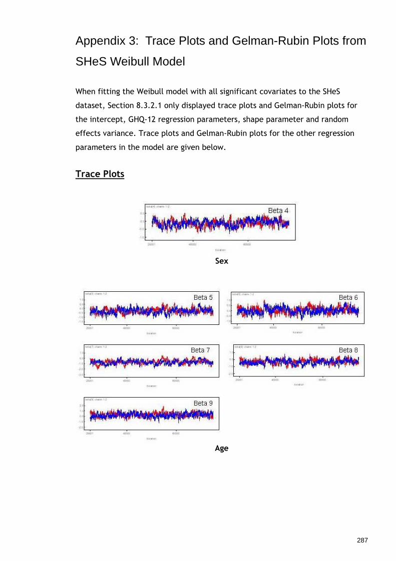
287
Appendix 3: Trace Plots and Gelman-Rubin Plots from
SHeS Weibull Model
When fitting the Weibull model with all significant covariates to the SHeS
dataset, Section 8.3.2.1 only displayed trace plots and Gelman-Rubin plots for
the intercept, GHQ-12 regression parameters, shape parameter and random
effects variance. Trace plots and Gelman-Rubin plots for the other regression
parameters in the model are given below.
Trace Plots
Sex
Age

288
Marital Status
Receipt of Benefits
Smoking Status
Employment Status
Self-Assessed General Health

289
Gelman-Rubin Plots
beta[4] chains 1:2
start-iteration
25251 40000
0.0 0.5 1.0 1.5 2.0
Sex
beta[5] chains 1:2
start-iteration
25251 40000
0.0
0.5
1.0
1.5
beta[6] chains 1:2
start-iteration
25251 40000
0.0
1.0
2.0
3.0
beta[7] chains 1:2
start-iteration
25251 40000
0.0
1.0
2.0
3.0
beta[8] chains 1:2
start-iteration
25251 40000
0.0
1.0
2.0
3.0
beta[9] chains 1:2
start-iteration
25251 40000
0.0
1.0
2.0
3.0
Age
beta[10] chains 1:2
start-iteration
25251 40000
0.0
0.5
1.0
1.5
Marital Status

290
beta[11] chains 1:2
start-iteration
25251 40000
0.0
0.5
1.0
1.5
Receipt of Benefits
beta[12] chains 1:2
start-iteration
25251 40000
0.0 0.5 1.0 1.5 2.0
beta[13] chains 1:2
start-iteration
25251 40000
0.0 1.0 2.0 3.0 4.0
Smoking Status
beta[14] chains 1:2
start-iteration
25251 40000
0.0
0.5
1.0
1.5
beta[15] chains 1:2
start-iteration
25251 40000
0.0
0.5
1.0
1.5
Employment Status
beta[16] chains 1:2
start-iteration
25251 40000
0.0
1.0
2.0
3.0
beta[17] chains 1:2
start-iteration
25251 40000
0.0
0.5
1.0
1.5
beta[18] chains 1:2
start-iteration
25251 40000
0.0
0.5
1.0
1.5
beta[19] chains 1:2
start-iteration
25251 40000
0.0
0.5
1.0
1.5
Self-Assessed General Health

291
Appendix 4: WinBUGS Code for Re-parameterised
Model with all Covariates
The WinBUGS code for the re-parameterised Weibull model containing all
significant covariates, i.e. the ‘full’ model, in Section 8.3.4 is given below.
Model for (i in 1:N) time[i] ~ dweib(r,mu[i])I(censor[i],) log(mu[i]) <- -r*log(lambda[i]) + u2[area[i]] # Random effects: for (j in 1:n2) u2[j] ~ dnorm(0.0, tau.u2) # Priors: loglambda1 ~ dnorm(0, 0.1) for (k in 1:19) loglambda2[k] ~ dnorm(0, 0.1) for (i in 1:N) loglambda[i] <- loglambda1 + loglambda2[1]*score_1_2[i] + loglambda2[2]*score_3_4[i] + loglambda2[3]*score_5_12[i] + loglambda2[4]*female[i] + loglambda2[5]*v25_34[i] + loglambda2[6]*v35_44[i]+ loglambda2[7]*v45_54[i] + loglambda2[8]*v55_64[i] + loglambda2[9]*v65_74[i] + loglambda2[10]*other_marital[i] + loglambda2[11]*yes_benefits[i] + loglambda2[12]*currentsmok[i] + loglambda2[13]*exsmok[i] + loglambda2[14]*unemployed[i] + loglambda2[15]*part_time[i] + loglambda2[16]*good[i] + loglambda2[17]*fair[i] + loglambda2[18]*bad[i] + loglambda2[19]*very_bad[i] lambda[i] <- exp(loglambda[i]) alpha <- -(r*loglambda1) beta[1] <- -(r*loglambda2[1]) beta[2] <- -(r*loglambda2[2]) beta[3] <- -(r*loglambda2[3]) beta[4] <- -(r*loglambda2[4]) beta[5] <- -(r*loglambda2[5]) beta[6] <- -(r*loglambda2[6]) beta[7] <- -(r*loglambda2[7]) beta[8] <- -(r*loglambda2[8]) beta[9] <- -(r*loglambda2[9]) beta[10] <- -(r*loglambda2[10]) beta[11] <- -(r*loglambda2[11]) beta[12] <- -(r*loglambda2[12]) beta[13] <- -(r*loglambda2[13]) beta[14] <- -(r*loglambda2[14]) beta[15] <- -(r*loglambda2[15]) beta[16] <- -(r*loglambda2[16]) beta[17] <- -(r*loglambda2[17]) beta[18] <- -(r*loglambda2[18]) beta[19] <- -(r*loglambda2[19]) # Priors for random effects variance sigma.u2~ dunif(0,3) sigma2.u2 <- sigma.u2*sigma.u2 tau.u2<-1/sigma2.u2

292
#Prior on shape parameter logr ~ dnorm(0, 0.1) r <-exp(logr)

293
Appendix 5: Discrete-Time Groupings for Swedish
Dataset
The following two tables display the discrete-time groupings of days used to
create the Swedish person-period dataset with 5 risk sets and 10 risk sets
respectively. The groupings for the person-period datasets with 3 and 7 risk sets
were given in Tables 9.5 and 9.6 respectively.
Discrete-time grouping for expanded dataset with 5 risk sets
Time Interval Grouping
1 2 3 4 5 6
Day 0 – day 1700 Day 1701 – day 2700 Day 2701 – day 4500 Day 4501 – day 6100 Day 6101 – day 8373 Day 8374 – day 8500
Note that, although there are 6 discrete-time intervals in the above table, the
last time interval contains only censored observations, and therefore was not
included as a risk set since no events occurred during that interval.
Discrete-time grouping for expanded dataset with 10 risk sets
Time Interval Grouping
1 2 3 4 5 6 7 8 9
10 11
Day 0 – day 900 Day 901 – day 1700
Day 1701 – day 2700 Day 2701 – day 3500 Day 3501 – day 4500 Day 4501 – day 5100 Day 5101 – day 6100 Day 6101 – day 6700 Day 6701 – day 7300 Day 7301 – day 8373 Day 8374 – day 8500
Note that, although there are 11 discrete-time intervals in the above table, the
last time interval contains only censored observations, and therefore was not

294
included as a risk set since no events occurred during that interval. Note that
the 9th and 10th risk sets contain information on events for individuals from the
older 1972 birth cohort only, as the last censored observation in the 1977 cohort
occurred at 6559 days from 12th birthday.

295
Appendix 6: Checking the Proportional Odds
Assumption in the Swedish Dataset
Section 7.2.3 noted that fitting discrete-time models requires a proportionality
assumption, which is referred to as the ‘proportional odds’ assumption if the
logit link function is adopted. As with the proportional hazards assumption, this
can be checked by including two-way interactions between covariates and time
in the model of interest in order to check that the effect of the covariate is the
same at all time points. A non-significant interaction implies the proportionality
assumption is reasonable.
The table below displays parameter estimates obtained from fitting a two-way
interaction between time and each of the fixed effects included in the discrete-
time ‘Individual+Area’ model fitted to the Swedish person-period dataset in
Section 9.4.2. Note that the two-way interactions were fitted one at a time and
not all at once. Note also that only the estimates for the interaction terms are
given here. For all other parameter estimates refer to Table 9.7. Since it was
already established in Table 9.8 that the effect of ‘cohort’ was not constant
over time, it is not necessary to check the proportionality assumption for this
variable again here. In order to cut down on the number of parameters to be
estimated, the models including the two-way interactions were fitted to the
person-period dataset with 3 risk sets. Although it was discussed that the
baseline hazard function wasn’t being estimated very accurately when there
were only 3 risk sets, it is hoped, nevertheless, that a rough indication of
whether or not the effects of the covariates are constant over time will be
obtained. Estimates were obtained using 2nd-order PQL.
Two-way interaction Estimate (s.e.) Sex*Time Male*Time 1 Female*Time 2 Female*Time 3
0.000 -0.547 (0.095) -1.022 (0.092)
Father Soc. Class*Time Employers etc*Time 1 Non-manual*Time 2 Manual*Time 2 Unclassifiable*Time 2 Non-manual*Time 3
0.000 0.207 (0.173) 0.184 (0.166) 0.050 (0.176) 0.024 (0.172)

296
Manual*Time 3 Unclassifiable*Time 3
0.204 (0.163) 0.251 (0.170)
Income Quintile*Time Quintile 1*Time 1 Quintile 2*Time 2 Quintile 3*Time 2 Quintile 4*Time 2 Quintile 5*Time 2 Missing*Time 2 Quintile 2*Time 3 Quintile 3*Time 3 Quintile 4*Time 3 Quintile 5*Time 3 Missing*Time 3
0.000 0.051 (0.136) 0.166 (0.142) -0.166 (0.143) 0.221 (0.156) 0.038 (0.175) -0.037 (0.132) 0.125 (0.137) -0.200 (0.139) -0.024 (0.156) -0.086 (0.172)
Housing Tenure*Time Owner Occupied*Time 1 Rented*Time 2 Rented*Time 3
0.000 -0.120 (0.089) 0.111 (0.087)
Economic Region*Time Metropolitan*Time 1 Larger Regional*Time 2 Smaller Regional*Time 2 Private Enterprise*Time 2 Public Sector*Time 2 Larger Regional*Time 3 Smaller Regional*Time 3 Private Enterprise*Time 3 Public Sector*Time 3
0.000 0.159 (0.099) -0.173 (0.145) -0.162 (0.233) 0.769 (0.321) 0.082 (0.098) -0.038 (0.136) -0.161 (0.226) 0.184 (0.352)
Generally, the proportional odds assumptions seem reasonable for the variables
‘father’s social class in 1980’, ‘household income quintile at birth’ and
‘economic region’. However, there are significant two-way interactions between
sex and time and housing tenure at birth and time, indicating that the
proportionality assumption is not valid for these variables. This would suggest
that these two-way interaction terms should be included in the final model.

297
Appendix 7: Fitting a Discrete-Time Model with Five
Risk Sets to the Swedish Dataset
Section 9.4.2 noted that discrete-time models were also fitted to a person-
period dataset containing 5 risk sets. A table indicating how the time intervals
were constructed to create the 5 risk sets is given in Appendix 5. Results from
fitting the ‘Individual’, ‘Individual+Area’ and ‘Full’ models to the Swedish data
are given in the table below. Parameter estimates should be compared to those
in Table 9.7. Models were estimated using 2nd-order PQL.
Varied Intervals with 5 Risk Sets
Individual Individual+Area Full Estimate (s.e.) Estimate (s.e.) Estimate (s.e.)
Fixed
Intercept (β0)
Time2 (α1) Time3 (α2) Time4 (α3) Time5 (α4)
Sex Male Female (β1)
Father Soc. Class 1980 Employers etc Non-manual (β2) Manual (β3) Unclassifiable (β4)
Hhold Income Quintile Quintile 1 Quintile 2 (β5) Quintile 3 (β6) Quintile 4 (β7) Quintile 5 (β8) Missing (β9)
Housing Tenure Owner Occupied Rented (β10)
Birth Cohort 1972 1977 (β11)
Economic Region Metropolitan Larger Regional (β12) Smaller Regional (β13) Private Enterprise(β14) Public Sector (β15)
-6.393 (0.080) -6.357 (0.090) -6.152 (0.108)
0.349 (0.058) 0.351 (0.062) 0.351 (0.062) 0.747 (0.054) 0.769 (0.057) 0.769 (0.057) 0.342 (0.054) 0.355 (0.062) 0.356 (0.062) -0.067 (0.064) -0.066 (0.068) -0.066 (0.068)
0.000 0.000 0.000 0.477 (0.035) 0.498 (0.037) 0.454 (0.049)
0.000 0.000 0.000 -0.110 (0.068) -0.104 (0.073) -0.177 (0.092) 0.165 (0.064) 0.166 (0.069) 0.134 (0.087) 0.580 (0.068) 0.559 (0.073) 0.484 (0.093)
0.000 0.000 0.000 -0.133 (0.052) -0.144 (0.056) -0.236 (0.073) -0.166 (0.054) -0.165 (0.057) -0.271 (0.076) -0.094 (0.056) -0.097 (0.060) -0.231 (0.080) -0.249 (0.064) -0.286 (0.068) -0.402 (0.087) 0.491 (0.068) 0.465 (0.072) 0.397 (0.095)
0.000 0.000 0.000 0.471 (0.037) 0.480 (0.039) 0.449 (0.051)
0.000 0.000 0.000 -0.024 (0.035) -0.037 (0.037) -0.514 (0.156)
0.000 0.000 -0.074 (0.043) -0.100 (0.056) -0.115 (0.061) -0.271 (0.083) 0.147 (0.099) 0.188 (0.123) -0.032 (0.133) -0.219 (0.187)
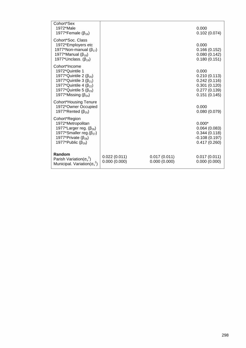
298
Cohort*Sex 1972*Male 1977*Female (β16)
Cohort*Soc. Class 1972*Employers etc 1977*Non-manual (β17) 1977*Manual (β18) 1977*Unclass. (β19)
Cohort*Income 1972*Quintile 1 1977*Quintile 2 (β20) 1977*Quintile 3 (β21) 1977*Quintile 4 (β22) 1977*Quintile 5 (β23) 1977*Missing (β24)
Cohort*Housing Tenure 1972*Owner Occupied 1977*Rented (β25)
Cohort*Region 1972*Metropolitan 1977*Larger reg. (β26) 1977*Smaller reg.(β27) 1977*Private (β28) 1977*Public (β29)
Random Parish Variation(σu
2) Municipal. Variation(σv
2)
0.000 0.102 (0.074)
0.000 0.166 (0.152) 0.080 (0.142) 0.180 (0.151)
0.000 0.210 (0.113) 0.242 (0.116) 0.301 (0.120) 0.277 (0.139) 0.151 (0.145)
0.000 0.080 (0.079)
0.000* 0.064 (0.083) 0.344 (0.118) -0.108 (0.197) 0.417 (0.260) 0.022 (0.011) 0.017 (0.011) 0.017 (0.011) 0.000 (0.000) 0.000 (0.000) 0.000 (0.000)

299
Appendix 8: Trace Plots and Gelman-Rubin Plots from
Swedish Weibull Model
When fitting the Weibull ‘Individual+Area’ model with all significant covariates
to the Swedish dataset, Section 9.4.4 only displayed trace plots and Gelman-
Rubin plots for the intercept, ‘cohort’ regression parameter, shape parameter
and random effects variance. Trace plots and Gelman-Rubin plots for the other
regression parameters in the model are given below.
Trace Plots
Sex
Father’s Social Class in 1980

300
Household Income Quintile at Birth
Housing Tenure at Birth
Economic Region

301
Gelman-Rubin Plots
beta[1] chains 1:2
start-iteration
10101 12500 15000 17500
0.0
1.0
2.0
3.0
Sex
beta[2] chains 1:2
start-iteration
10101 12500 15000 17500
0.0 0.5 1.0 1.5 2.0
beta[3] chains 1:2
start-iteration
10101 12500 15000 17500
0.0 0.5 1.0 1.5 2.0
beta[4] chains 1:2
start-iteration
10101 12500 15000 17500
0.0 0.5 1.0 1.5 2.0
Father’s Social Class in 1980

302
beta[5] chains 1:2
start-iteration
10101 12500 15000 17500
0.0
1.0
2.0
3.0
beta[6] chains 1:2
start-iteration
10101 12500 15000 17500
0.0
1.0
2.0
3.0
beta[7] chains 1:2
start-iteration
10101 12500 15000 17500
0.0
0.5
1.0
1.5
beta[8] chains 1:2
start-iteration
10101 12500 15000 17500
0.0
0.5
1.0
1.5
beta[9] chains 1:2
start-iteration
10101 12500 15000 17500
0.0
0.5
1.0
1.5
Household Income at Birth
beta[10] chains 1:2
start-iteration
10101 12500 15000 17500
0.0
0.5
1.0
1.5
Housing Tenure at Birth
beta[12] chains 1:2
start-iteration
10101 12500 15000 17500
0.0
1.0
2.0
3.0
beta[13] chains 1:2
start-iteration
10101 12500 15000 17500
0.0 0.5 1.0 1.5 2.0
beta[14] chains 1:2
start-iteration
10101 12500 15000 17500
0.0 0.5 1.0 1.5 2.0
beta[15] chains 1:2
start-iteration
10101 12500 15000 17500
0.0 0.5 1.0 1.5 2.0
Economic Region

303
Appendix 9: WinBUGS code for the Weibull Model
with Different Shape Parameters
The WinBUGS code for the Weibull model with shape parameter defined
separately for each cohort is given below.
model for (i in 1:N) time[i] ~ dweib(r[cohort_77[i]+1],mu[i]) I(censor[i],) log(mu[i]) <- alpha + beta[1] * Female[i] + beta[2] * Non_manual_workers[i] + beta[3] * Manual_workers[i] + beta[4] * Unclassifiable_and_missing[i] + beta[5] * hh_incbth_2[i] + beta[6] * hh_incbth_3[i] + beta[7] * hh_incbth_4[i] + beta[8] * hh_incbth_5[i] + beta[9] * hh_incbth_miss[i] + beta[10] * rented[i] + beta[11] * cohort_77[i] + beta[12] * Larger_regional_centres[i] + beta[13] * Smaller_regional_centres[i] + beta[14] * Small_regions___mostly_private_enterprises[i] + beta[15] * Small_regions___mostly_public_sector[i] + u2[parbth[i]] for (j in 1:n2) u2[j] ~ dnorm(0.0, tau.u2) # Priors: alpha ~ dnorm(0.0, 0.0001) for (k in 1:15) beta[k] ~ dnorm(0.0, 0.0001) logr[1] ~ dnorm(0, 0.1) logr[2] ~ dnorm(0, 0.1) r[1] <-exp(logr[1]) r[2] <-exp(logr[2]) # Priors for random effects variance sigma.u2~ dunif(0,3) sigma2.u2 <- sigma.u2*sigma.u2 tau.u2<-1/sigma2.u2
304
References
1. Hosmer, D.W. and S. Lemeshow, Applied Survival Analysis: Regression Modeling of Time to Event Data. 1999: John Wiley & Sons, Inc.Canada.
2. Diez Roux, A.V., Invited commentary: Places, people, and health. American Journal of Epidemiology, 2002. 155(6): p. 516-519.
3. Diez-Roux, A.V., Bringing context back into epidemiology: Variables and fallacies in multilevel analysis. American Journal of Public Health, 1998. 88(2): p. 216-222.
4. Petronis, K.R. and J.C. Anthony, A different kind of contextual effect: geographical clustering of cocaine incidence in the USA. Journal of Epidemiology and Community Health, 2003. 57(11): p. 893-900.
5. Macintyre, S., A. Ellaway, and S. Cummins, Place effects on health: how can we conceptualise, operationalise and measure them? Social Science & Medicine, 2002. 55(1): p. 125-139.
6. Vonkorff, M., T. Koepsell, S. Curry, and P. Diehr, Multilevel Analysis in Epidemiologic Research on Health Behaviors and Outcomes. American Journal of Epidemiology, 1992. 135(10): p. 1077-1082.
7. Leyland, A.H. and P.P. Groenewegen, Multilevel modelling and public health policy. Scandinavian Journal of Public Health, 2003. 31(4): p. 267-274.
8. Pearce, N., The ecological fallacy strikes back. Journal of Epidemiology and Community Health, 2000. 54(5): p. 326-327.
9. Diez Roux, A.V., Investigating neighborhood and area effects on health. American Journal of Public Health, 2001. 91(11): p. 1783-9.
10. Duncan, C., K. Jones, and G. Moon, Health-related behaviour in context: A multilevel modelling approach. Social Science & Medicine, 1996. 42(6): p. 817-830.
11. Duncan, C., K. Jones, and G. Moon, Context, composition and heterogeneity: Using multilevel models in health research. Social Science & Medicine, 1998. 46(1): p. 97-117.
12. Merlo, J., B. Chaix, M. Yang, J. Lynch, and L. Rastam, A brief conceptual tutorial of multilevel analysis in social epidemiology: linking the statistical concept of clustering to the idea of contextual phenomenon. Journal of Epidemiology and Community Health, 2005. 59(6): p. 443-449.
13. Rice, N. and A. Leyland, Multilevel models: applications to health data. Journal of Health Services Research & Policy, 1996. 1(3): p. 154-64.
14. Skinner, C.J. and D. Holt, Analysis of Complex Surveys, ed. T.M.F. Smith. 1989: John Wiley & Sons Inc.
15. Greenland, S., Principles of multilevel modelling. International Journal of Epidemiology, 2000. 29(1): p. 158-167.
16. Jones, K., Specifying and Estimating Multilevel Models for Geographical Research. Transactions of the Institute of British Geographers, 1991. 16(2): p. 148-159.
17. O'Campo, P., Invited commentary: Advancing theory and methods for multilevel models of residential neighborhoods and health. American Journal of Epidemiology, 2003. 157(1): p. 9-13.
18. Pickett, K.E. and M. Pearl, Multilevel analyses of neighbourhood socioeconomic context and health outcomes: a critical review. Journal of Epidemiology and Community Health, 2001. 55(2): p. 111-122.

305
19. Sullivan, L.M., K.A. Dukes, and E. Losina, Tutorial in biostatistics - An introduction to hierarchical linear modelling. Statistics in Medicine, 1999. 18(7): p. 855-888.
20. Rasbash, J., C. Charlton, W. Browne, M.J.R. Healy, and B. Cameron. MLwiN Version 2.02. 2005 [cited; Available from: http://www.cmm.bristol.ac.uk/MLwiN/index.shtml.
21. Imperial College and MRC, U. WinBUGS with DoodleBUGS Version 1.4.3. 2007 [cited; Available from: http://www.mrc-bsu.cam.ac.uk/bugs/welcome.shtml.
22. Gray, L., G.D. Batty, P. Craig, C. Stewart, B. Whyte, A. Finlayson, and A.H. Leyland, Cohort Profile: The Scottish Health Surveys Cohort: linkage of study participants to routinely collected records for mortality, hospital discharge, cancer and offspring birth characteristics in three nationwide studies. International Journal of Epidemiology, 2009: p. dyp155.
23. Scottish Executive Health Department, Scotland's Health: Scottish Health Survey 1995, W. Dong and B. Erins, Editors. 1997.
24. Economic and Social Data Service. The Scottish Health Survey SMR1/SMR4/Cancers/Deaths Linked Datasets. [cited 2007; Available from: http://www.esds.ac.uk/government/shes/.
25. Scottish Executive Health Department, The Scottish Health Survey 1998, A. Shaw, A. McMunn, and J. Field, Editors. 2000, Joint Health Surveys Unit at The National Centre for Social Research and Department of Epidemiology & Public Health, UCL.
26. McLoone, P., Carstairs scores for Scottish postcode sectors from the 2001 Census. 2004, Medical Research Council Social & Public Health Sciences Unit.
27. Lawder, R., A. Elders, and D. Clark. Using the linked Scottish Health Survey to predict hospitalisation and death: an analysis of the link between behavioural, biological and social risk factors and subsequent hospital admission and death in Scotland. 2007 [cited; Available from: http://www.scotpho.org.uk/nmsruntime/saveasdialog.asp?lID=4018&sID=3480.
28. Craig, P. The Scottish Health Survey-Scottish Morbidity Record Linked Datasets: Introduction to a new resource. [cited 2010; Powerpoint Presentation]. Available from: www.ccsr.ac.uk/esds/events/2008-07-08/petercraig.ppt.
29. Kendrick, S. The Development of Record Linkage in Scotland: The Responsive Application of Probability Matching. [cited 2010 June]; Available from: http://www.fcsm.gov/working-papers/skendrick.pdf.
30. Stewart, C., Risk Factors for Psychiatric Hospital Admissions in Scotland, in Public Health. 2006, University of Glasgow: Glasgow.
31. Naidoo, J. and J. Wills, Health Promotion: Foundations for Practice. 2nd ed. 2000, Edinburgh: Bailliere Tindall.
32. Hannah, M. and M. Halliday, With Health in Mind: Improving mental health and wellbeing in Scotland, S. Platt, Editor. 2002, The Scottish Public Mental Health Alliance.
33. Well Scotland. Scotland's Mental Health. [cited 2009; Available from: http://www.wellscotland.info/mentalhealth/.
34. Scottish Association for Mental Health. What's It Worth? The Social and Economic Costs of Mental Health Problems in Scotland. [cited 2009; Available from: http://www.samh.org.uk/assets/files/112.pdf.

306
35. Scottish Association for Mental Health. Working it Out: A Guide to Managing Mental Health in the Workplace. [cited 2009; Available from: http://www.samh.org.uk/assets/files/273.pdf.
36. Scottish Public Health Observatory. Mental health: introduction. [cited 2010; Available from: http://www.scotpho.org.uk/home/Healthwell-beinganddisease/MentalHealth/mental_intro.asp.
37. Mental Health Foundation. Mental health - an overview. [cited 2010; Available from: http://www.mentalhealth.org.uk/information/mental-health-overview/.
38. World Health Organisation, Integrating mental health into primary care: A global perspective. 2008, World Health Organisation.
39. Scottish Executive, National Programme for Improving Mental Health and Well-Being: Action plan 2003-2006. 2003, Scottish Executive.
40. Well Scotland. About the National Programme. [cited 2010; Available from: http://www.wellscotland.info/mentalhealth/national-programme.html.
41. Prince, M., V. Patel, S. Saxena, M. Maj, J. Maselko, M.R. Phillips, and A. Rahman, Global mental health 1 - No health without mental health. Lancet, 2007. 370(9590): p. 859-877.
42. Information and Services Division Scotland. Mental Health: Hospital Inpatients. [cited 2009; Available from: http://www.isdscotland.org/isd/information-and-statistics.jsp?pContentID=1220&p_applic=CCC&p_service=Content.show&.
43. Information and Services Division Scotland, Mental illness specialities; inpatient admissions by speciality - Year ending 31st March 2007. 2008.
44. Information and Services Division Scotland. Mental Health Statistical Publication Notice: Mental Health (Psychiatric) Hospital Activity Statistics. 2008 [cited 2009; Available from: http://www.isdscotland.org/isd/5694.html.
45. Lewis, G. and R.I. Araya, Is the General Health Questionnaire (12 Item) a Culturally Biased Measure of Psychiatric-Disorder. Social Psychiatry and Psychiatric Epidemiology, 1995. 30(1): p. 20-25.
46. Vanhemert, A.M., M. Denheijer, M. Vorstenbosch, and J.H. Bolk, Detecting Psychiatric-Disorders in Medical-Practice Using the General Health Questionnaire - Why Do Cutoff Scores Vary. Psychological Medicine, 1995. 25(1): p. 165-170.
47. Schmitz, N., J. Kruse, and W. Tress, Improving screening for mental disorders in the primary care setting by combining the GHQ-12 and SCL-90-R subscales. Comprehensive Psychiatry, 2001. 42(2): p. 166-173.
48. Goldberg, D.P. and P. Williams, A User's Guide to the General Health Questionnaire 1991: NFER-Nelson.
49. Hardy, G.E., D.A. Shapiro, C.E. Haynes, and J.E. Rick, Validation of the general health questionnaire-12 using a sample of employees from England's health care services. Psychological Assessment, 1999. 11(2): p. 159-165.
50. Goldberg, D.P., R. Gater, N. Sartorius, T.B. Ustun, M. Piccinelli, O. Gureje, and C. Rutter, The validity of two versions of the GHQ in the WHO study of mental illness in general health care. Psychological Medicine, 1997. 27(01): p. 191-197.
51. Donath, S., The validity of the 12-item General Health Questionnaire in Australia: a comparison between three scoring methods. Australian and New Zealand Journal of Psychiatry, 2001. 35(2): p. 231-235.

307
52. Holi, M.M., M. Marttunen, and V. Aalberg, Comparison of the GHQ-36, the GHQ-12 and the SCL-90 as psychiatric screening instruments in the Finnish population. Nordic Journal of Psychiatry, 2003. 57(3): p. 233-238.
53. Bartlett, C.J. and E.C. Coles, Psychological health and well-being: why and how should public health specialists measure it? Part 1: rationale and methods of the investigation, and review of psychiatric epidemiology. Journal of Public Health Medicine, 1998. 20(3): p. 281-287.
54. Schmitz, N., J. Kruse, and W. Tress, Application of stratum-specific likelihood ratios in mental health screening. Social Psychiatry and Psychiatric Epidemiology, 2000. 35(8): p. 375-379.
55. Willmott, S.A., J.A.P. Boardman, C.A. Henshaw, and P.W. Jones, Understanding General Health Questionnaire (GHQ-28) score and its threshold. Social Psychiatry and Psychiatric Epidemiology, 2004. 39(8): p. 613-617.
56. Hennekens, C.H. and J.E. Buring, Epidemiology in Medicine, ed. S.L. Mayrent. 1987, Philadelphia: Lippincott Williams & Wilkins.
57. Goldberg, D.P., T. Oldehinkel, and J. Ormel, Why GHQ threshold varies from one place to another. Psychological Medicine, 1998. 28(4): p. 915-921.
58. Lahelma, E., M. Laaksonen, P. Martikainen, O. Rahkonen, and S. Sarlio-Lahteenkorva, Multiple measures of socioeconomic circumstances and common mental disorders. Social Science & Medicine, 2006. 63(5): p. 1383-1399.
59. Finlayjones, R.A. and E. Murphy, Severity of Psychiatric-Disorder and the 30-Item General Health Questionnaire. British Journal of Psychiatry, 1979. 134(JUN): p. 609-616.
60. Schmitz, N., J. Kruse, C. Heckrath, L. Alberti, and W. Trees, Diagnosing mental disorders in primary care: the General Health Questionnaire (GHQ) and the Symptom Check List (SCL-90-R) as screening instruments. Social Psychiatry and Psychiatric Epidemiology, 1999. 34(7): p. 360-366.
61. Bushnell, J., D. McLeod, A. Dowell, C. Salmond, S. Ramage, S. Collings, P. Ellis, M. Kljakovic, and L. McBain, The effectiveness of case-finding for mental health problems in primary care. British Journal of General Practice, 2005. 55(518): p. 665-669.
62. Banks, M.H., C.W. Clegg, P.R. Jackson, N.J. Kemp, E.M. Stafford, and T.D. Wall, The Use of the General Health Questionnaire as an Indicator of Mental-Health in Occupational Studies. Journal of Occupational Psychology, 1980. 53(3): p. 187-194.
63. Mari, J.D. and P. Williams, Misclassification by Psychiatric Screening Questionnaires. Journal of Chronic Diseases, 1986. 39(5): p. 371-378.
64. Araya, R., R. Wynn, and G. Lewis, Comparison of 2 Self Administered Psychiatric Questionnaires (Ghq-12 and Srq-20) in Primary Care in Chile. Social Psychiatry and Psychiatric Epidemiology, 1992. 27(4): p. 168-173.
65. Fox, J.W., Sex, Marital-Status, and Age as Social Selection Factors in Recent Psychiatric-Treatment. Journal of Health and Social Behavior, 1984. 25(4): p. 394-405.
66. Jarman, B., S. Hirsch, P. White, and R. Driscoll, Predicting Psychiatric Admission Rates. British Medical Journal, 1992. 304(6835): p. 1146-1151.
67. Gove, W.R., Gender Differences in Mental and Physical Illness - the Effects of Fixed Roles and Nurturant Roles. Social Science & Medicine, 1984. 19(2): p. 77-91.
68. Zent, M.R., Sex and Mental Disorder - a Reappraisal. Sociological Focus, 1984. 17(2): p. 121-136.

308
69. Emslie, C., R. Fuhrer, K. Hunt, S. Macintyre, M. Shipley, and S. Stansfeld, Gender differences in mental health: evidence from three organisations. Social Science & Medicine, 2002. 54(4): p. 621-624.
70. Yip, K.S., Gender differences in mental illness in Hong Kong. Administration and Policy in Mental Health, 2003. 30(4): p. 361-368.
71. Jenkins, R., Sex-Differences in Minor Psychiatric Morbidity - a Survey of a Homogeneous Population. Social Science & Medicine, 1985. 20(9): p. 887-899.
72. Kirshner, L.A. and L. Johnston, Effects of Gender on Inpatient Psychiatric-Hospitalization. Journal of Nervous and Mental Disease, 1983. 171(11): p. 651-657.
73. Timms, D., Gender, social mobility and psychiatric diagnoses. Social Science & Medicine, 1998. 46(9): p. 1235-1247.
74. Saarento, O., S. Rasanen, P. Nieminen, H. Hakko, and M. Isohanni, Sex differences in the contact rates and utilization of psychiatric services. A three-year follow-up study in northern Finland. European Psychiatry, 2000. 15(3): p. 205-212.
75. Thompson, A., M. Shaw, G. Harrison, D. Ho, D. Gunnell, and J. Verne, Patterns of hospital admission for adult psychiatric illness in England: analysis of Hospital Episode Statistics data. The British Journal of Psychiatry, 2004. 185(4): p. 334-341.
76. Rushing, W.A., Marital-Status and Mental Disorder - Evidence in Favor of a Behavioral-Model. Social Forces, 1979. 58(2): p. 540-556.
77. Mattioni, T., D. Di Lallo, R. Roberti, M. Miceli, M. Stefani, C. Maci, and C.A. Perucci, Determinants of psychiatric inpatient admission to general hospital psychiatric wards: an epidemiological study in a region of central Italy. Social Psychiatry and Psychiatric Epidemiology, 1999. 34(8): p. 425-31.
78. Martin, W.T., Status Integration, Social Stress, and Mental-Illness - Accounting for Marital-Status Variations in Mental Hospitalization Rates. Journal of Health and Social Behavior, 1976. 17(3): p. 280-294.
79. Robertson, N.C., The Relationship Between Marital Status and the Risk of Psychiatric Referral. The British Journal of Psychiatry, 1974. 124(2): p. 191-202.
80. Lavik, N.J., Marital-Status in Psychiatric-Patients. Acta Psychiatrica Scandinavica, 1982. 65(1): p. 15-28.
81. Adler, L.M., The Relationship of Marital Status to Incidence of and Recovery from Mental Illness. Social Forces, 1953. 32(2): p. 185-194.
82. Tweed, D.L. and D.J. Jackson, Psychiatric-Disorder and Gender - a Logit Analysis. Social Forces, 1981. 59(4): p. 1200-1216.
83. Halldin, J., Prevalence of Mental Disorder in an Urban-Population in Central Sweden in Relation to Social-Class, Marital-Status and Immigration. Acta Psychiatrica Scandinavica, 1985. 71(2): p. 117-127.
84. Gove, W.R., Sex differences in the epidemiology of mental disorder: Evidence and explanations, in Gender and disordered behaviour, E.S. Gomberg and V. Franks, Editors. 1979, Brunner/Mazel: New York.
85. Gold, J.H., Gender differences in psychiatric illness and treatments - A critical review. Journal of Nervous and Mental Disease, 1998. 186(12): p. 769-775.
86. Kessler, R.C., A Disaggregation of the Relationship between Socio-Economic Status and Psychological Distress. American Sociological Review, 1982. 47(6): p. 752-764.
309
87. Koppel, S. and P. McGuffin, Socio-economic factors that predict psychiatric admissions at a local level. Psychological Medicine, 1999. 29(5): p. 1235-1241.
88. Rushing, W.A. and S.T. Ortega, Socioeconomic-Status and Mental Disorder - New Evidence and a Sociomedical Formulation. American Journal of Sociology, 1979. 84(5): p. 1175-1200.
89. Thornicroft, G., Social Deprivation and Rates of Treated Mental Disorder - Developing Statistical-Models to Predict Psychiatric-Service Utilization. British Journal of Psychiatry, 1991. 158: p. 475-484.
90. Fryers, T., D. Melzer, and R. Jenkins, Social inequalities and the common mental disorders - A systematic review of the evidence. Social Psychiatry and Psychiatric Epidemiology, 2003. 38(5): p. 229-237.
91. Rodgers, B., Socioeconomic-Status, Employment and Neurosis. Social Psychiatry and Psychiatric Epidemiology, 1991. 26(3): p. 104-114.
92. Weich, S., R. Churchill, G. Lewis, and A. Mann, Do socio-economic risk factors predict the incidence and maintenance of psychiatric disorder in primary care? Psychological Medicine, 1997. 27(01): p. 73-80.
93. Dohrenwend, B.P., Sociocultural and Social-Psychological Factors in Genesis of Mental-Disorders. Journal of Health and Social Behavior, 1975. 16(4): p. 365-392.
94. Weich, S. and G. Lewis, Material standard of living, social class, and the prevalence of the common mental disorders in Great Britain. Journal of Epidemiology and Community Health, 1998. 52(1): p. 8-14.
95. Skapinakis, P., S. Weich, G. Lewis, N. Singleton, and R. Araya, Socio-economic position and common mental disorders - Longitudinal study in the general population in the UK. British Journal of Psychiatry, 2006. 189: p. 109-117.
96. Kammerling, R.M. and S. Oconnor, Unemployment Rate as Predictor of Rate of Psychiatric Admission. British Medical Journal, 1993. 307(6918): p. 1536-1539.
97. Dekker, J., J. Peen, A. Goris, H. Heijnen, and H. Kwakman, Social deprivation and psychiatric admission rates in Amsterdam. Social Psychiatry and Psychiatric Epidemiology, 1997. 32(8): p. 485-492.
98. Belek, I., Social class, income, education, area of residence and psychological distress: does social class have an independent effect on psychological distress in Antalya, Turkey? Social Psychiatry and Psychiatric Epidemiology, 2000. 35(2): p. 94-101.
99. Galobardes, B., M. Shaw, D.A. Lawlor, J.W. Lynch, and G.D. Smith, Indicators of socioeconomic position (part 1). Journal of Epidemiology and Community Health, 2006. 60(1): p. 7-12.
100. Working Group on Inequalities and Health, G.B., Inequalities in Health: The Black Report: The Health Divide, ed. P. Townsend. 1988: Penguin Books.
101. Warr, P., Work, Unemployment and Mental Health. 1987: Clarendon Press.
102. Carter, K.N., T. Blakely, S. Collings, F.I. Gunasekara, and K. Richardson, What is the association between wealth and mental health? Journal of Epidemiology and Community Health, 2009. 63(3): p. 221-226.
103. Lopes, F.L., I. Nascimento, W.A. Zin, A.M. Valenca, M.A. Mezzasalma, I. Figueira, and A.E. Nardi, Smoking and psychiatric disorders: a comorbidity survey. Brazilian Journal of Medical and Biological Research, 2002. 35(8): p. 961-967.

310
104. Peto, R., A.D. Lopez, J. Boreham, M. Thun, and C. Heath, Mortality from Tobacco in Developed-Countries - Indirect Estimation from National Vital-Statistics. Lancet, 1992. 339(8804): p. 1268-1278.
105. Cuijpers, P., F. Smit, M. ten Have, and R. de Graaf, Smoking is associated with first-ever incidence of mental disorders: a prospective population-based study. Addiction, 2007. 102(8): p. 1303-1309.
106. Breslau, N., S.P. Novak, and R.C. Kessler, Daily smoking and the subsequent onset of psychiatric disorders. Psychological Medicine, 2004. 34(2): p. 323-333.
107. Araya, R., J. Gaete, G. Rojas, R. Fritsch, and G. Lewis, Smoking and common mental disorders: a population-based survey in Santiago, Chile. Social Psychiatry and Psychiatric Epidemiology, 2007. 42(11): p. 874-880.
108. Rasul, F., S.A. Stansfeld, G. Davey-Smith, C.L. Hart, and C. Gillis, Sociodemographic factors, smoking and common mental disorder in the Renfrew and Paisley (MIDSPAN) study. Journal of Health Psychology, 2001. 6(2): p. 149-158.
109. Faulkner, G. and S. Biddle, Exercise and mental health: It's just not psychology! Journal of Sports Sciences, 2001. 19(6): p. 433-444.
110. Burbach, F.R., The efficacy of physical activity interventions within mental health services: Anxiety and depressive disorders. Journal of Mental Health, 1997. 6(6): p. 543.
111. Fox, K.R., The influence of physical activity on mental well-being. Public Health Nutrition, 1999. 2(3A): p. 411-8.
112. Paffenbarger, R.S., I.M. Lee, and R. Leung, Physical activity and personal characteristics associated with depression and suicide in American college men. Acta Psychiatrica Scandinavica, 1994. 89(s377): p. 16-22.
113. Taylor, A.H. and G. Faulkner, Inaugural editorial. Mental Health and Physical Activity, 2008. 1(1): p. 1-8.
114. Bernadt, M.W. and R.M. Murray, Psychiatric-Disorder, Drinking and Alcoholism - What Are the Links. British Journal of Psychiatry, 1986. 148: p. 393-400.
115. Andreasson, S. and P. Allebeck, Alcohol and Psychiatric-Illness - Longitudinal-Study of Psychiatric Admissions in a Cohort of Swedish Conscripts. International Journal of the Addictions, 1991. 26(6): p. 713-728.
116. Arillo-Santillan, E., E. Lazcano-Ponce, M. Hernandez-Avila, E. Fernandez, B. Allen, R. Valdes, and J. Samet, Associations between individual and contextual factors and smoking in 13,293 Mexican students. American Journal of Preventive Medicine, 2005. 28(1): p. 41-51.
117. Winkelstein, W., Epidemiological Considerations Underlying Allocation of Health and Disease Care Resources. International Journal of Epidemiology, 1972. 1(1): p. 69-74.
118. Silver, E., E.P. Mulvey, and J.W. Swanson, Neighborhood structural characteristics and mental disorder: Faris and Dunham revisited. Social Science & Medicine, 2002. 55(8): p. 1457-1470.
119. Weich, S., L. Twigg, G. Holt, G. Lewis, and K. Jones, Contextual risk factors for the common mental disorders in Britain: a multilevel investigation of the effects of place. Journal of Epidemiology and Community Health, 2003. 57(8): p. 616-621.
120. Propper, C., K. Jones, A. Bolster, S. Burgess, R. Johnston, and R. Sarker, Local neighbourhood and mental health: Evidence from the UK. Social Science & Medicine, 2005. 61(10): p. 2065-2083.

311
121. Dupere, V. and D.D. Perkins, Community types and mental health: a multilevel study of local environmental stress and coping. American Journal of Community Psychology, 2007. 39(1-2): p. 107-119.
122. Fone, D., F. Dunstan, G. Williams, K. Lloyd, and S. Palmer, Places, people and mental health: A multilevel analysis of economic inactivity. Social Science & Medicine, 2007. 64(3): p. 633-645.
123. Peterson, L.E., A.C. Tsai, S. Petterson, and D.G. Litaker, Rural-urban comparison of contextual associations with self-reported mental health status. Health & Place, 2009. 15(1): p. 125-132.
124. Weich, S., G. Holt, L. Twigg, K. Jones, and G. Lewis, Geographic variation in the prevalence of common mental disorders in Britain: A multilevel investigation. American Journal of Epidemiology, 2003. 157(8): p. 730-737.
125. Goldsmith, H.F., C.E. Holzer, and R.W. Manderscheid, Neighborhood characteristics and mental illness. Evaluation and Program Planning, 1998. 21(2): p. 211-225.
126. Paykel, E.S., R. Abbott, R. Jenkins, T.S. Brugha, and H. Meltzer, Urban-rural mental health differences in Great Britain: findings from the National Morbidity Survey. Psychological Medicine, 2000. 30(2): p. 269-280.
127. Sundquist, K., G. Frank, and J. Sundquist, Urbanisation and incidence of psychosis and depression - Follow-up study of 4.4 million women and men in Sweden. British Journal of Psychiatry, 2004. 184: p. 293-298.
128. Allardyce, J., H. Gilmour, J. Atkinson, T. Rapson, J. Bishop, and R.G. McCreadie, Social fragmentation, deprivation and urbanicity: relation to first-admission rates for psychoses. British Journal of Psychiatry, 2005. 187: p. 401-406.
129. Chaix, B., J. Merlo, S.V. Subramanian, J. Lynch, and P. Chauvin, Comparison of a spatial perspective with the multilevel analytical approach in neighborhood studies: The case of mental and behavioral disorders due to psychoactive substance use in Malmo, Sweden, 2001. American Journal of Epidemiology, 2005. 162(2): p. 171-182.
130. Reijneveld, S.A. and A.H. Schene, Higher prevalence of mental disorders in socioeconomically deprived urban areas in the Netherlands: Community or personal disadvantage? Journal of Epidemiology and Community Health, 1998. 52(1): p. 2-7.
131. Harrison, J., S. Barrow, and F. Creed, Mental health in the North West Region of England: associations with deprivation. Social Psychiatry and Psychiatric Epidemiology, 1998. 33(3): p. 124-128.
132. Driessen, G., N. Gunther, and J. Van Os, Shared social environment and psychiatric disorder: a multilevel analysis of individual and ecological effects. Social Psychiatry and Psychiatric Epidemiology, 1998. 33(12): p. 606-612.
133. Fone, D.L., K. Lloyd, and F.D. Dunstan, Measuring the neighbourhood using UK benefits data: a multilevel analysis of mental health status. Bmc Public Health, 2007. 7.
134. Curtis, S., A. Copeland, J. Fagg, P. Congdon, M. Almog, and J. Fitzpatrick, The ecological relationship between deprivation, social isolation and rates of hospital admission for acute psychiatric care: a comparison of London and New York City. Health & Place, 2006. 12(1): p. 19-37.
135. Drukker, M., G. Driessen, L. Krabbendam, and J. van Os, The wider social environment and mental health service use. Acta Psychiatrica Scandinavica, 2004. 110(2): p. 119-129.

312
136. Fone, D., F. Dunstan, K. Lloyd, G. Williams, J. Watkins, and S. Palmer, Does social cohesion modify the association between area income deprivation and mental health? A multilevel analysis. International Journal of Epidemiology, 2007. 36(2): p. 338-345.
137. Wainwright, N.W.J. and P.G. Surtees, Places, people, and their physical and mental functional health. Journal of Epidemiology and Community Health, 2004. 58(4): p. 333-339.
138. Skapinakis, P., G. Lewis, R. Araya, K. Jones, and G. Williams, Mental health inequalities in Wales, UK: multi-level investigation of the effect of area deprivation. British Journal of Psychiatry, 2005. 186: p. 417-422.
139. Weich, S., L. Twigg, G. Lewis, and K. Jones, Geographical variation in rates of common mental disorders in Britain: prospective cohort study. British Journal of Psychiatry, 2005. 187: p. 29-34.
140. Fone, D.L. and F. Dunstan, Mental health, places and people: A multilevel analysis of economic inactivity and social deprivation. Health & Place, 2006. 12(3): p. 332-344.
141. Duncan, C., K. Jones, and G. Moon, Psychiatric Morbidity - a Multilevel Approach to Regional Variations in the Uk. Journal of Epidemiology and Community Health, 1995. 49(3): p. 290-295.
142. Chaix, B., A.H. Leyland, C.E. Sabel, P. Chauvin, L. Rastam, H. Kristersson, and J. Merlo, Spatial clustering of mental disorders and associated characteristics of the neighbourhood context in Malmo, Sweden, in 2001. Journal of Epidemiology and Community Health, 2006. 60(5): p. 427-435.
143. Thomas, H., N. Weaver, J. Patterson, P. Jones, T. Bell, R. Playle, F. Dunstan, S. Palmer, G. Lewis, and R. Araya, Mental health and quality of residential environment. British Journal of Psychiatry, 2007. 191: p. 500-505.
144. Fayers, P.M., D. Curran, and D. Machin, Incomplete quality of life data in randomized trials: Missing items. Statistics in Medicine, 1998. 17(5-7): p. 679-696.
145. Kline, R.B., Principles and Practice of Structural Equation Modeling. 1998: The Guilford Press.
146. Musil, C.M., C.B. Warner, P.K. Yobas, and S.L. Jones, A comparison of imputation techniques for handling missing data. Western Journal of Nursing Research, 2002. 24(7): p. 815-829.
147. SPSSInc., SPSS 14.0 for Windows. 2005. 148. Acock, A.C., Working with missing values. Journal of Marriage and the
Family, 2005. 67(4): p. 1012-1028. 149. McCullagh, P. and J.A. Nelder, Generalized Linear Models. Second Edition
ed. 1989: Chapman and Hall. 150. Rasbash, J., F. Steele, W.J. Browne, and H. Goldstein. A User's Guide to
MLwiN, v2.10. 2009 [cited; Available from: http://www.cmm.bristol.ac.uk/MLwiN/download/MLwiN-userman-09.pdf.
151. Snijders, T. and R. Bosker, Multilevel Analysis: An introduction to basic and advanced multilevel modelling. 1999: SAGE Publications.
152. Goldstein, H., W. Browne, and J. Rasbash, Partitioning Variation in Multilevel Models. Understanding Statistics, 2002. 1(4): p. 223.
153. Rice, N., Multilevel Modelling of Health Statistics, ed. A.H. Leyland and H. Goldstein. 2001: Wiley. pp.28 - 31.
154. Huppert, F.A. and J.E. Whittington, Symptoms of Psychological Distress Predict 7-Year Mortality. Psychological Medicine, 1995. 25(5): p. 1073-1086.
313
155. Robinson, K.L., J. McBeth, and G.J. MacFarlane, Psychological distress and premature mortality in the general population: A prospective study. Annals of Epidemiology, 2004. 14(7): p. 467-472.
156. Allison, P.D., Discrete-Time Methods for the Analysis of Event Histories. Sociological Methodology, 1982. 13: p. 61-98.
157. Petersen, T., The Statistical-Analysis of Event Histories. Sociological Methods & Research, 1991. 19(3): p. 270-323.
158. Kalbfleisch, J.D. and R.L. Prentice, The Statistical Analysis of Failure Time Data. Second Edition ed. 2002: Wiley.
159. Cox, D.R. and D. Oakes, Analysis of Survival Data. 1984: Chapman and Hall.
160. Klein, J.P. and M.L. Moeschberger, Survival Analysis: Techniques for Censored and Truncated Data. 1997: Springer.
161. Hougaard, P., Analysis of Multivariate Survival Data. 2000: Springer. 162. Orbe, J., E. Ferreira, and V. Nunez-Anton, Comparing proportional
hazards and accelerated failure time models for survival analysis. Statistics in Medicine, 2002. 21(22): p. 3493-3510.
163. Yang, M. and H. Goldstein. Modelling survival data in MLwiN 1.20. 2003 [cited; Available from: http://www.cmm.bristol.ac.uk/MLwiN/download/msdm.pdf.
164. Patel, K., R. Kay, and L. Rowell, Comparing proportional hazards and accelerated failure time models: an application in influenza. Pharmaceutical Statistics, 2006. 5(3): p. 213-224.
165. Skrondal, A. and S. Rabe-Hesketh, Generalised Latent Variable Modelling: Multilevel, Longitudinal and Structural Equation Models. 2004: Chapman & Hall/CRC.
166. Goldstein, H., Multilevel Statistical Models. Second Edition ed. 1995: Arnold.
167. Kelly, P.J., A review of software packages for analyzing correlated survival data. American Statistician, 2004. 58(4): p. 337-342.
168. Whitehead, J., Fitting Cox's Regression Model to Survival Data using GLIM. Journal of the Royal Statistical Society. Series C (Applied Statistics), 1980. 29(3): p. 268-275.
169. Ma, R.J., D. Krewski, and R.T. Burnett, Random effects Cox models: A Poisson modelling approach. Biometrika, 2003. 90(1): p. 157-169.
170. Hess, K.R., Graphical Methods for Assessing Violations of the Proportional Hazards Assumption in Cox Regression. Statistics in Medicine, 1995. 14(15): p. 1707-1723.
171. Goldstein, H., Multilevel Mixed Linear-Model Analysis Using Iterative Generalized Least-Squares. Biometrika, 1986. 73(1): p. 43-56.
172. Goldstein, H. and J. Rasbash, Efficient Computational Procedures for the Estimation of Parameters in Multilevel Models Based on Iterative Generalized Least-Squares. Computational Statistics & Data Analysis, 1992. 13(1): p. 63-71.
173. Goldstein, H., Restricted Unbiased Iterative Generalized Least-Squares Estimation. Biometrika, 1989. 76(3): p. 622-623.
174. Steele, F., S.L. Curtis, and M. Choe, The impact of family planning service provision on contraceptive-use dynamics in Morocco. Studies in Family Planning, 1999. 30(1): p. 28-42.
175. Rodriguez, G. and N. Goldman, An Assessment of Estimation Procedures for Multilevel Models with Binary Responses. Journal of the Royal Statistical Society Series a-Statistics in Society, 1995. 158: p. 73-89.

314
176. Callas, P.W., H. Pastides, and D.W. Hosmer, Empirical comparisons of proportional hazards, Poisson, and logistic regression modeling of occupational cohort data. American Journal of Industrial Medicine, 1998. 33(1): p. 33-47.
177. Yang, M., S. Eldridge, and J. Merlo, Multilevel survival analysis of health inequalities in life expectancy. International Journal for Equity in Health, 2009. 8: p. 31.
178. Schootman, M., D.B. Jeffe, M. Lian, W.E. Gillanders, and R. Aft, The Role of Poverty Rate and Racial Distribution in the Geographic Clustering of Breast Cancer Survival Among Older Women: A Geographic and Multilevel Analysis. American Journal of Epidemiology, 2009. 169(5): p. 554-561.
179. Roberts, A., The influences of incident and contextual characteristics on crime clearance of nonlethal violence: A multilevel event history analysis. Journal of Criminal Justice, 2008. 36(1): p. 61-71.
180. Chaix, B., M. Rosvall, and J. Merlo, Assessment of the magnitude of geographical variations and socioeconomic contextual effects on ischaemic heart disease mortality: a multilevel survival analysis of a large Swedish cohort. Journal of Epidemiology and Community Health, 2007. 61(4): p. 349-355.
181. Chaix, B., M. Rosvall, and J. Merlo, Recent increase of neighborhood socioeconomic effects on ischemic heart disease mortality: A multilevel survival analysis of two large Swedish cohorts. American Journal of Epidemiology, 2007. 165(1): p. 22-26.
182. Shih, J.H. and S.E. Lu, Analysis of failure time data with multilevel clustering, with application to the child vitamin a intervention trial in Nepal. Biometrics, 2007. 63(3): p. 673-680.
183. Dejardin, O., L. Remontet, A.M. Bouvier, A. Danzon, B. Tretarre, P. Delafosse, F. Molinie, N. Maarouf, M. Velten, E.A. Sauleau, N. Bourdon-Raverdy, P. Grosclaude, S. Boutreux, G. De Pouvourville, and G. Launoy, Socioeconomic and geographic determinants of survival of patients with digestive cancer in France. British Journal of Cancer, 2006. 95(7): p. 944-949.
184. Kravdal, O., Does place matter for cancer survival in Norway? A multilevel analysis of the importance of hospital affiliation and municipality socio-economic resources. Health & Place, 2006. 12(4): p. 527-537.
185. Merlo, J., P.O. Ostergren, K. Broms, A. Bjorck-Linne, and H. Liedholm, Survival after initial hospitalisation for heart failure: a multilevel analysis of patients in Swedish acute care hospitals. Journal of Epidemiology and Community Health, 2001. 55(5): p. 323-329.
186. Dawson, D.A., Drinking as a risk factor for sustained smoking. Drug and Alcohol Dependence, 2000. 59(3): p. 235-249.
187. Romberger, D.J. and K. Grant, Alcohol consumption and smoking status: the role of smoking cessation. Biomedicine & Pharmacotherapy, 2004. 58(2): p. 77-83.
188. Kahler, C.W., R. Borland, A. Hyland, S.A. McKee, M.E. Thompson, and K.M. Cummings, Alcohol consumption and quitting smoking in the International Tobacco Control (ITC) Four Country Survey. Drug and Alcohol Dependence, 2009. 100(3): p. 214-220.
189. Shohaimi, S., R. Luben, N. Wareham, N. Day, S. Bingham, A. Welch, S. Oakes, and K.T. Khaw, Residential area deprivation predicts smoking habit independently of individual educational level and occupational social class. A cross sectional study in the Norfolk cohort of the European

315
Investigation into Cancer (EPIC-Norfolk). Journal of Epidemiology and Community Health, 2003. 57(4): p. 270-276.
190. Laaksonen, M., O. Rahkonen, S. Karvonen, and E. Lahelma, Socioeconomic status and smoking. European Journal of Public Health, 2005. 15(3): p. 262-269.
191. Harwood, G.A., P. Salsberry, A.K. Ferketich, and A.E. Wewers, Cigarette smoking, socioeconomic status, and psychosocial factors: Examining a conceptual framework. Public Health Nursing, 2007. 24(4): p. 361-371.
192. Schaap, M.M., H.M.E. van Agt, and A.E. Kunst, Identification of socioeconomic groups at increased risk for smoking in European countries: Looking beyond educational level. Nicotine & Tobacco Research, 2008. 10(2): p. 359-369.
193. Odegard, O., Marriage and Mental Disease : A Study in Social Psychopathology. Journal of Mental Science, 1946. 92(386): p. 35-59.
194. Dohrenwend, B.P., Socioeconomic-Status (Ses) and Psychiatric-Disorders - Are the Issues Still Compelling. Social Psychiatry and Psychiatric Epidemiology, 1990. 25(1): p. 41-47.
195. Kassel, J.D., L.R. Stroud, and C.A. Paronis, Smoking, stress, and negative affect: Correlation, causation, and context across stages of smoking. Psychological Bulletin, 2003. 129(2): p. 270-304.
196. Gove, W.R., The Relationship between Sex Roles, Marital Status, and Mental Illness. Social Forces, 1972. 51(1): p. 34-44.
197. Almog, M., S. Curtis, A. Copeland, and P. Congdon, Geographical variation in acute psychiatric admissions within New York City 1990-2000: growing inequalities in service use? Social Science & Medicine, 2004. 59(2): p. 361-376.
198. Manda, S. and R. Meyer, Age at first marriage in Malawi: a Bayesian multilevel analysis using a discrete time-to-event model. Journal of the Royal Statistical Society Series a-Statistics in Society, 2005. 168: p. 439-455.
199. Reardon, S.F., R.T. Brennan, and S.L. Buka, Estimating multi-level discrete-time hazard models using cross-sectional data: Neighborhood effects on the onset of adolescent cigarette use. Multivariate Behavioral Research, 2002. 37(3): p. 297-330.
200. Biggeri, L., M. Bini, and L. Grilli, The transition from university to work: a multilevel approach to the analysis of the time to obtain the first job. Journal of the Royal Statistical Society Series a-Statistics in Society, 2001. 164: p. 293-305.
201. Paccagnella, O., Comparing vocational training courses through a discrete-time multilevel hazard model. Statistical Modelling, 2006. 6(2): p. 119-139.
202. McCullagh, P., Regression-Models for Ordinal Data. Journal of the Royal Statistical Society Series B-Methodological, 1980. 42(2): p. 109-142.
203. Hedeker, D., O. Siddiqui, and F.B. Hu, Random-effects regression analysis of correlated grouped-time survival data. Statistical Methods in Medical Research, 2000. 9(2): p. 161-179.
204. Willett, J.B. and J.D. Singer, Investigating Onset, Cessation, Relapse, and Recovery - Why You Should, and How You Can, Use Discrete-Time Survival Analysis to Examine Event Occurrence. Journal of Consulting and Clinical Psychology, 1993. 61(6): p. 952-965.
205. Hank, K., Regional social contexts and individual fertility decisions: A multilevel analysis of first and second births in Western Germany.
316
European Journal of Population-Revue Europeenne De Demographie, 2002. 18(3): p. 281-299.
206. Yamaguchi, K., Event History Analysis. Applied Social Research Methods Series. Vol. 28. 1991: Sage Publications.
207. Browne, W.J., F. Steele, M. Golalizadeh, and M.J. Green, The use of simple reparameterizations to improve the efficiency of Markov chain Monte Carlo estimation for multilevel models with applications to discrete time survival models. Journal of the Royal Statistical Society : Series A, 2009. 172(3): p. 579-598.
208. Steele, F., H. Goldstein, and W. Browne, A general multilevel multistate competing risks model for event history data, with an application to a study of contraceptive use dynamics. Statistical Modelling, 2004. 4(2): p. 145-159.
209. Diamond, I.D., J.W. McDonald, and I.H. Shah, Proportional Hazards Models for Current Status Data - Application to the Study of Differentials in Age at Weaning in Pakistan. Demography, 1986. 23(4): p. 607-620.
210. Gamerman, D. and H.F. Lopes, Markov Chain Monte Carlo: Stochastic Simulation for Bayesian Inference. Second Edition ed. 2006: Chapman & Hall/CRC, Taylor & Francis Group.
211. Wong, M.C.M., K.F. Lam, and E.C.M. Lo, Multilevel modelling of clustered grouped survival data using Cox regression model: an application to ART dental restorations. Statistics in Medicine, 2006. 25(3): p. 447-457.
212. Browne, W.J. and D. Draper, A comparison of Bayesian and likelihood-based methods for fitting multilevel models. Bayesian Analysis, 2006. 1(3): p. 473-513.
213. Dellaportas, P. and A.F.M. Smith, Bayesian-Inference for Generalized Linear and Proportional Hazards Models Via Gibbs Sampling. Applied Statistics-Journal of the Royal Statistical Society Series C, 1993. 42(3): p. 443-459.
214. Sargent, D.J., A general framework for random effects survival analysis in the cox proportional hazards setting. Biometrics, 1998. 54(4): p. 1486-1497.
215. Vaupel, J.W., K.G. Manton, and E. Stallard, Impact of Heterogeneity in Individual Frailty on the Dynamics of Mortality. Demography, 1979. 16(3): p. 439-454.
216. Clayton, D.G., Model for Association in Bivariate Life Tables and Its Application in Epidemiological-Studies of Familial Tendency in Chronic Disease Incidence. Biometrika, 1978. 65(1): p. 141-151.
217. Guo, G.A. and G. Rodriguez, Estimating a Multivariate Proportional Hazards Model for Clustered Data Using the Em Algorithm, with an Application to Child Survival in Guatemala. Journal of the American Statistical Association, 1992. 87(420): p. 969-976.
218. Hougaard, P., Frailty models for survival data. Lifetime Data Analysis, 1995. 1(3): p. 255-73.
219. Gutierrez, R.G., Parametric frailty and shared frailty survival models. Stata Journal, 2002. 2(1): p. 22-44.
220. Ripatti, S. and J. Palmgren, Estimation of multivariate frailty models using penalized partial likelihood. Biometrics, 2000. 56(4): p. 1016-1022.
221. Ibrahim, J.G., M.-H. Chen, and S. Debajyoti, Bayesian Survival Analysis. 2001, New York: Springer.
222. Korsgaard, I.R., P. Madsen, and J. Jensen, Bayesian inference in the semiparametric log normal frailty model using Gibbs sampling. Genetics Selection Evolution, 1998. 30(3): p. 241-256.
317
223. Do Ha, I. and Y. Lee, Estimating frailty models via Poisson hierarchical generalized linear models. Journal of Computational and Graphical Statistics, 2003. 12(3): p. 663-681.
224. Rondeau, V., L. Filleul, and P. Joly, Nested frailty models using maximum penalized likelihood estimation. Statistics in Medicine, 2006. 25(23): p. 4036-4052.
225. Locatelli, I., P. Lichtenstein, and A.I. Yashin, A Bayesian correlated frailty model applied to Swedish breast cancer data, in MPIDR Working Paper WP 2003-025. 2003, Max Planck Institute for Demographic Research.
226. Petersen, J.H., P.K. Andersen, and R.D. Gill, Variance components models for survival data. Statistica Neerlandica, 1996. 50(1): p. 193-211.
227. Shih, J.H. and T.A. Louis, Assessing gamma frailty models for clustered failure time data, in Lifetime Data: Models in Reliability and Survival Analysis, N.P. Jewell, et al., Editors. 1996, Kluwer Academic Publ: Dordrecht. p. 299-305.
228. Sastry, N., A nested frailty model for survival data, with an application to the study of child survival in northeast Brazil. Journal of the American Statistical Association, 1997. 92(438): p. 426-435.
229. Manda, S.O.M., A comparison of methods for analysing a nested frailty model to child survival in Malawi. Australian & New Zealand Journal of Statistics, 2001. 43(1): p. 7-16.
230. Clayton, D.G., A Monte-Carlo Method for Bayesian-Inference in Frailty Models. Biometrics, 1991. 47(2): p. 467-485.
231. Gustafson, P., Large hierarchical Bayesian analysis of multivariate survival data. Biometrics, 1997. 53(1): p. 230-242.
232. Matsuyama, Y., J. Sakamoto, and Y. OhashI, A Bayesian hierarchical survival model for the institutional effects in a multi-centre cancer clinical trial. Statistics in Medicine, 1998. 17(17): p. 1893-1908.
233. Wienke, A., K.G. Arbeev, I. Locatelli, and A.I. Yashin, A comparison of different bivariate correlated frailty models and estimation strategies. Mathematical Biosciences, 2005. 198(1): p. 1-13.
234. Dossantos, D.M., R.B. Davies, and B. Francis, Nonparametric Hazard Versus Nonparametric Frailty Distribution in Modeling Recurrence of Breast-Cancer. Journal of Statistical Planning and Inference, 1995. 47(1-2): p. 111-127.
235. Walker, S.G. and B.K. Mallick, Hierarchical generalized linear models and frailty models with Bayesian nonparametric mixing. Journal of the Royal Statistical Society Series B-Methodological, 1997. 59(4): p. 845-860.
236. Naskar, M., Semiparametric analysis of clustered survival data under nonparametric frailty. Statistica Neerlandica, 2008. 62(2): p. 155-172.
237. Lavine, M., Some Aspects of Polya Tree Distributions for Statistical Modeling. Annals of Statistics, 1992. 20(3): p. 1222-1235.
238. Lavine, M., More Aspects of Polya Tree Distributions for Statistical Modelling. The Annals of Statistics, 1994. 22(3): p. 1161-1176.
239. Mauldin, R.D., W.D. Sudderth, and S.C. Williams, Polya Trees and Random Distributions. The Annals of Statistics, 1992. 20(3): p. 1203-1221.
240. Glidden, D.V. and E. Vittinghoff, Modelling clustered survival data from multicentre clinical trials. Statistics in Medicine, 2004. 23(3): p. 369-388.
241. Klein, J.P., Semiparametric Estimation of Random Effects Using the Cox Model Based on the Em Algorithm. Biometrics, 1992. 48(3): p. 795-806.
242. Sinha, D. and D.K. Dey, Semiparametric Bayesian analysis of survival data. Journal of the American Statistical Association, 1997. 92(439): p. 1195-1212.

318
243. Egleston, B.L. Lecture 6: Weibull Survival Probability Distribution. [cited 2009; Available from: http://www.biostat.jhsph.edu/~beglesto/survfiles/weibull.pdf.
244. Sahu, K.S., Dey, D.K., Aslanidou, H, Sinha, D, A Weibull Regression Model with Gamma Frailties for Multivariate Survival Data. Lifetime Data Analysis, 1997. 3: p. 123-137.
245. Spiegelhalter, D.J., A. Thomas, N.G. Best, and D. Lunn, WinBUGS User Manual Version 1.4. 2003.
246. Lambert, P.C., A.J. Sutton, P.R. Burton, K.R. Abrams, and D.R. Jones, How vague is vague? A simulation study of the impact of the use of vague prior distributions in MCMC using WinBUGS. Statistics in Medicine, 2005. 24(15): p. 2401-2428.
247. Brooks, S.P., Markov chain Monte Carlo method and its application. Journal of the Royal Statistical Society Series D-the Statistician, 1998. 47(1): p. 69-100.
248. Scurrah, K.J., L.J. Palmer, and P.R. Burton, Variance components analysis for pedigree-based censored survival data using generalized linear mixed models (GLMMs) and Gibbs sampling in BUGS. Genetic Epidemiology, 2000. 19(2): p. 127-148.
249. Gilks, W.R., S. Richardson, and D.J. Spiegelhalter, Markov Chain Monte Carlo in Practice. 1998: Chapman & Hall/CRC.
250. Smith, A.F.M. and G.O. Roberts, Bayesian Computation Via the Gibbs Sampler and Related Markov-Chain Monte-Carlo Methods. Journal of the Royal Statistical Society Series B-Methodological, 1993. 55(1): p. 3-23.
251. Brooks, S.P. and G.O. Roberts, Convergence assessment techniques for Markov chain Monte Carlo. Statistics and Computing, 1998. 8(4): p. 319-335.
252. Jackman, S., Estimation and inference via Bayesian simulation: An introduction to Markov Chain Monte Carlo. American Journal of Political Science, 2000. 44(2): p. 375-404.
253. Kass, R.E., B.P. Carlin, A. Gelman, and R.M. Neal, Markov chain Monte Carlo in practice: A roundtable discussion. American Statistician, 1998. 52(2): p. 93-100.
254. Vines, S.K., W.R. Gilks, and P. Wild, Fitting Bayesian multiple random effects models. Statistics and Computing, 1996. 6(4): p. 337-346.
255. Cowles, M.K. and B.P. Carlin, Markov chain Monte Carlo convergence diagnostics: A comparative review. Journal of the American Statistical Association, 1996. 91(434): p. 883-904.
256. Gelman, A. and D. Rubin, Inference from Iterative Simulation Using Multiple Sequences. Statistical Science, 1992. 7(4): p. 457-472.
257. Brooks, S.P. and A. Gelman, General methods for monitoring convergence of iterative simulations. Journal of Computational and Graphical Statistics, 1998. 7(4): p. 434-455.
258. Gelman, A., Parameterization and Bayesian modeling. Journal of the American Statistical Association, 2004. 99(466): p. 537-545.
259. Brighton Webs Ltd. Weibull Distribution (Two Parameter). [cited 2010; Available from: http://www.brighton-webs.co.uk/distributions/weibull2.asp.
260. Liu, C.H., D.B. Rubin, and Y.N. Wu, Parameter expansion to accelerate EM: The PX-EM algorithm. Biometrika, 1998. 85(4): p. 755-770.
261. Liu, J.S. and Y.N. Wu, Parameter expansion for data augmentation. Journal of the American Statistical Association, 1999. 94(448): p. 1264-1274.

319
262. Browne, W., An Illustration of the Use of Reparameterisation Methods for Improving MCMC Efficiency in Crossed Random Effect Models, in Multilevel Modelling Newsletters. 2004.
263. Casellas, J., Bayesian inference in a piecewise Weibull proportional hazards model with unknown change points. Journal of Animal Breeding and Genetics, 2007. 124(4): p. 176-184.
264. Tarres, J., J. Casellas, and J. Piedrafita, Genetic and environmental factors influencing mortality up to weaning of Bruna dels Pirineus beef calves in mountain areas. A survival analysis. Journal of Animal Science, 2005. 83(3): p. 543-551.
265. Steele, F., I. Diamond, and D.L. Wang, The determinants of the duration of contraceptive use in China: A multilevel multinomial discrete-hazards modeling approach. Demography, 1996. 33(1): p. 12-23.
266. Goldstein, H., H. Pan, and J. Bynner, A Flexible Procedure for Analyzing Longitudinal Event Histories Using a Multilevel Model. Understanding Statistics, 2004. 3(2): p. 85 - 99.