Multilevel Modeling WorkshopMultilevel Modeling WorkshopUniversity of KentuckyUniversity of Kentucky

Brandon BartelsBrandon BartelsGeorge Washington UniversityGeorge Washington University

May 23May 23--25, 201125, 2011

Introduction• Exciting methodological toolkit

• Multilevel modeling is not monolithic– There are lots of different types of model specifications that fall

under the umbrella.

– Various specifications carry different substantive interpretations.

OutlineI. Motivation and Core Issues

II. Linear variance components model

III. Random intercept model (aka, random effects model) and itsalternatives (e.g., OLS, fixed effects, “between” effects)

IV. Cluster confounding

V. Applications to longitudinal (panel/time-series cross-sectional) data

VI. Random coefficient model

VII. Nonlinear models for noncontinuous dependent variables

I. Motivation and Core Issues

Multilevel Data• Contain multiple levels of analysis, with each level consisting

of distinct units of analysis.

• Most common form of multilevel data: hierarchical data. – Two-level structure: Units from the lowest level of analysis

(level-1 units) are nested withinunits from a higher level of analysis (level-2 units)

• Data are “clustered”

• Level-2 units are referred to as “clusters”

– Three-level structure: Third level is present

Multilevel Data• Examples

– Education: students (level-1 units) nested within schools (level-2 units)

• Three levels: students nested within schools nested within states

– Individuals nested within cities– Voters nested within congressional districts– Voters nested within time (or temporal contexts)– Panel data and time-series cross-sectional (TSCS) data

• What’s a sufficient number of level-2 units, or clusters? – Rough guideline: >15

• What’s a sufficient number for cluster sizes (number of observations per cluster/level-2 unit)? – Cluster sizes can vary; at least 2 and more like >5 (rough

guideline)

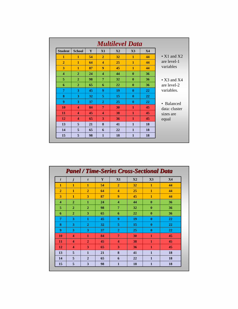
Multilevel DataStudent School Y X1 X2 X3 X4

1 1 54 2 32 1 44

2 1 64 4 25 1 44

3 1 87 9 45 1 44

4 2 24 4 44 0 36

5 2 98 7 32 0 36

6 2 65 6 22 0 36

7 3 45 9 19 0 22

8 3 32 5 15 0 22

9 3 37 2 25 0 22

10 4 84 7 30 1 45

11 4 45 4 38 1 45

12 4 65 3 36 1 45

13 5 21 8 41 1 18

14 5 65 6 22 1 18

15 5 98 1 18 1 18

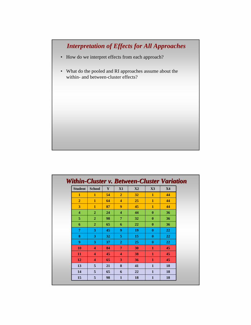
• X1 and X2 are level-1 variables

• X3 and X4 are level-2 variables.

• Balanced data: cluster sizes are equal

Panel / TimePanel / Time--Series CrossSeries Cross--Sectional DataSectional Datai j t Y X1 X2 X3 X4

1 1 1 54 2 32 1 44

2 1 2 64 4 25 1 44

3 1 3 87 9 45 1 44

4 2 1 24 4 44 0 36

5 2 2 98 7 32 0 36

6 2 3 65 6 22 0 36

7 3 1 45 9 19 0 22

8 3 2 32 5 15 0 22

9 3 3 37 2 25 0 22

10 4 1 84 7 30 1 45

11 4 2 45 4 38 1 45

12 4 3 65 3 36 1 45

13 5 1 21 8 41 1 18

14 5 2 65 6 22 1 18

15 5 3 98 1 18 1 18

Motivation• Types of phenomena we’re interested in are multilayered and

complex.– Incorporating these layers enhances our substantive explanations

of phenomena.

• People don’t make choices or behave in a vacuum; there’s a context in which they act.

• This contextual, or situational, variation may have consequences for how people behave.

• Most simple cross-sectional data ignores this structure; “naïve pooling”

Motivation• Parsing explained variance in the dependent variable between

individual versus aggregatelevels of analysis. – Student versus school effects on performance.

Key TopicsKey Topics1. Unobserved heterogeneity(in the dependent variable)

– Between-cluster heterogeneity in the dependent variable

• Unobserved factors specific to each cluster that influence the dependent variable; factors are shared by observations within each cluster.

• Unmeasured, unobserved, and unimagined differences between clusters.

– Method: Random intercept models (aka, random effects)

– UH in a cross-sectional context:

yi = b0 + b1x1i + b2x2i + ei

UH in Hierarchical ContextUH in Hierarchical Context

Key TopicsKey Topics2. Pooling

– Degree to which parameters (e.g., intercept, effects of IVs) are“pulled” toward the pooled (global) effect or reflect within-cluster variation.

Spectrum:

No Partial Pooling Complete

Pooling ------------------------------------------- Pooling

3. Distinguish within-cluster, between-cluster, and total variation– “Cluster confounding”

Within-Cluster v. Between-Cluster VariationStudent School Y X1 X2 X3 X4

1 1 54 2 32 1 44

2 1 64 4 25 1 44

3 1 87 9 45 1 44

4 2 24 4 44 0 36

5 2 98 7 32 0 36

6 2 65 6 22 0 36

7 3 45 9 19 0 22

8 3 32 5 15 0 22

9 3 37 2 25 0 22

10 4 84 7 30 1 45

11 4 45 4 38 1 45

12 4 65 3 36 1 45

13 5 21 8 41 1 18

14 5 65 6 22 1 18

15 5 98 1 18 1 18

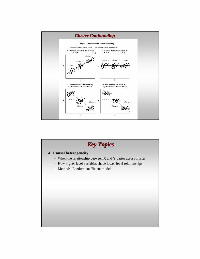
Cluster ConfoundingCluster Confounding

Key TopicsKey Topics4. Causal heterogeneity

– When the relationship between X and Y varies across cluster

– How higher level variables shape lower-level relationships.

– Methods: Random coefficient models

II. Linear Variance Components Model

Modeling Clustered DataModeling Clustered Data

• We’ll start simple: No independent variables

• Linear variance components model

• We’ll focus on making inferences about cluster means, i.e., mean of Y for each level-2 unit.

PoolingPooling• Degree to which each cluster mean is “pulled” toward the

overall, global mean.

Spectrum:

No Partial Pooling Complete

Pooling ------------------------------------------- Pooling

• Important questions:– What does each approach imply?

– Under what conditions would we want to rely on each type when making inferences about cluster means?

PoolingPooling

Modeling Clustered DataModeling Clustered Data• No Pooling:

– Within-clustercentral tendency and variation are all that matter.

– Between-clustervariation ignored.

– Generalize (in terms of means of the DV) one cluster at a time (in isolation) using cluster means

– Estimation technique: Fixed-effects (within) estimator

• Complete Pooling:– Ignores clustering/hierarchical structure. – Doesn’t distinguish within- versus between-cluster variation – Generalization: “Global mean” or “grand mean”

• Balanced data: mean of DV over entire sample• Unbalanced data: mean of the cluster means

– Estimation technique: Plain-vanilla pooled regression (e.g., OLS)

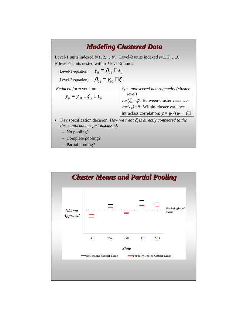
Modeling Clustered DataModeling Clustered Data• Partial Pooling:

– Weighted averagebetween no pooling and complete pooling extremes.

• Borrows information from completely pooled mean to generate refined estimate of cluster mean (think about “uninformative” clusters)

– Partially-pooled estimates of cluster meansare going to be weighted averages of the “no pooling cluster means”and the “completely-pooled mean of the cluster means.”

– Estimation technique: random intercept (aka, random effects) model

– Considerations affecting the degree of partial pooling?

Modeling Clustered DataModeling Clustered DataLevel-1 units indexed i=1, 2, …N. Level-2 units indexed j=1, 2, …J.

N level-1 units nested within J level-2 units.

jj

ijjijy

ζγβεβ

+=

+=

000

0[Level-1 equation]

[Level-2 equation]

ijjijy εζγ ++= 00

Reduced formversion:

• Key specification decision: How we treat ζj is directly connected to the three approaches just discussed.

– No pooling?

– Complete pooling?

– Partial pooling?

ζj = unobserved heterogeneity (cluster level)

var(ζi)=ψ : Between-cluster variance.

var(εij)=θ : Within-cluster variance.

Intraclass correlation: ρ = ψ / (ψ + θ)

Cluster Means and Partial PoolingCluster Means and Partial Pooling

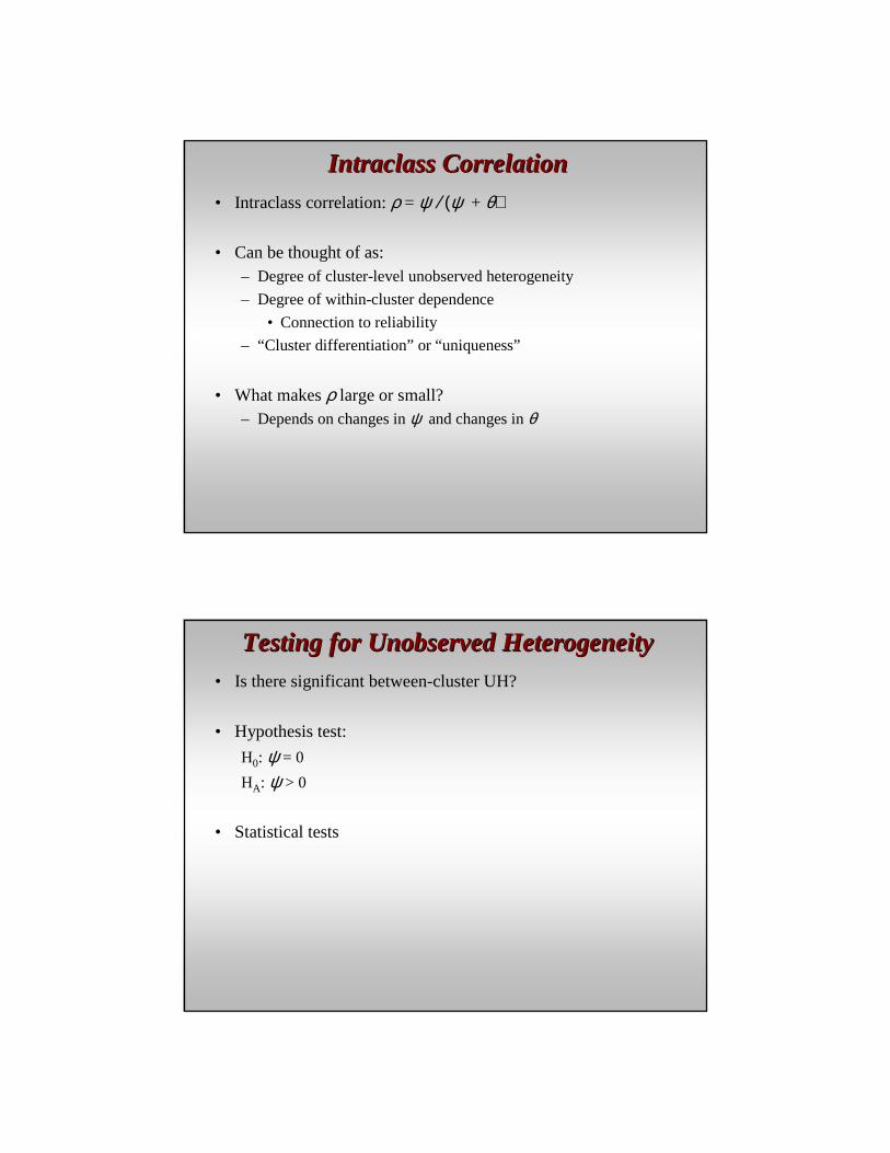
IntraclassIntraclass CorrelationCorrelation• Intraclass correlation: ρ = ψ / (ψ + θ)

• Can be thought of as: – Degree of cluster-level unobserved heterogeneity

– Degree of within-cluster dependence

• Connection to reliability

– “Cluster differentiation” or “uniqueness”

• What makes ρ large or small?– Depends on changes in ψ and changes in θ

Testing for Unobserved HeterogeneityTesting for Unobserved Heterogeneity• Is there significant between-cluster UH?

• Hypothesis test:

H0: ψ = 0

HA: ψ > 0

• Statistical tests

Shrinkage and Pooling in Random Intercept Shrinkage and Pooling in Random Intercept ModelModel

• Shrinkage and pooling are directly related. – The “weight” that determines how much the within-cluster means are

pulled toward the pooled mean

• Shrinkage is the degree to which ζj’s (level-2 residuals) are pulled toward zero; centers on estimating ζj’s.

• Pooling is the degree to which the cluster means gravitate toward the global mean of Y.– Gives us deeper insight into how much unobserved heterogeneity there

is in the dependent variable.

• Recall that the variance components model (random intercept model w/no IVs) allows for partial poolingof the cluster means.

• We can calculate the degree of partial poolingusing a “pooling factor.”

Generating PartiallyGenerating Partially--Pooled LevelPooled Level--2 Residuals2 Residuals

• Level-2 residuals from the partially-pooled approach reflect how much each cluster deviates from the global mean.

• Partially pooled level-2 residuals are called “empirical Bayes”(EB) residuals, which uses the “prior” distribution of ζ [ζ ~ N(0, ψ)], combined with the “data” (how informative the clusters are individually) to generate a “posterior” prediction of ζ (partially-pooled prediction).

• The smaller ψ is, the more informative the prior and the more it will drag the predicted ζ toward 0, which is the mean of the prior distribution (hence, “shrinkage”).

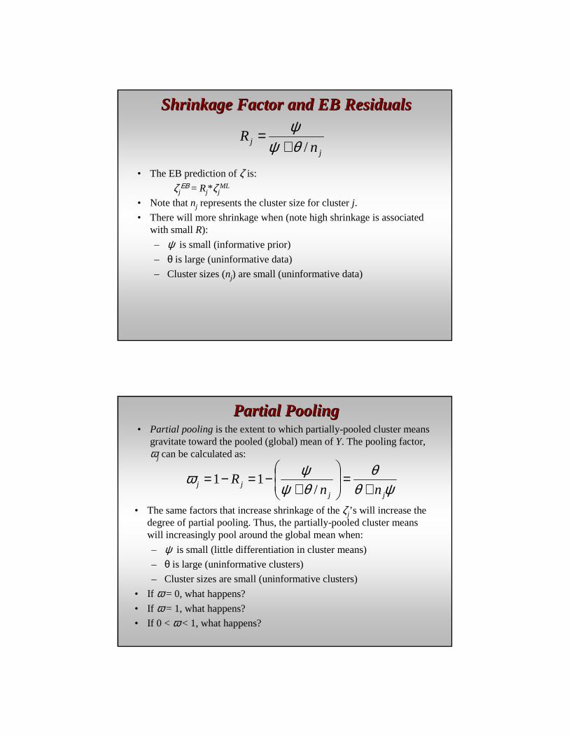
Shrinkage Factor and EB ResidualsShrinkage Factor and EB Residuals

jj n

R/θψ

ψ+

=

• The EB prediction of ζ is:

ζjΕΒ = Rj*ζj

ML

• Note that nj represents the cluster size for cluster j.

• There will more shrinkage when (note high shrinkage is associated with small R):

– ψ is small (informative prior)

– θ is large (uninformative data)

– Cluster sizes (nj) are small (uninformative data)

Partial PoolingPartial Pooling• Partial poolingis the extent to which partially-pooled cluster means

gravitate toward the pooled (global) mean of Y. The pooling factor, ωj can be calculated as:

ψθθ

θψψω

jjjj nn

R+

=

+−=−=

/11

• The same factors that increase shrinkage of the ζj’s will increase the degree of partial pooling. Thus, the partially-pooled cluster means will increasingly pool around the global mean when:

– ψ is small (little differentiation in cluster means)

– θ is large (uninformative clusters)

– Cluster sizes are small (uninformative clusters)

• If ω = 0, what happens?

• If ω = 1, what happens?

• If 0 < ω < 1, what happens?

PoolingPooling• Shrinkage and pooling factors can be calculated using our

model results; note that all we need are the variance estimates at each level and the cluster size(s).

• Pooling factors for balanced versus unbalanced data….– Balanced?

– In unbalanced data, how will variation in cluster size influencethe degree of pooling? How and why?

Calculating PartiallyCalculating Partially--Pooled Cluster MeansPooled Cluster Means

• We can use our estimates of pooling factors to calculate partially-pooled estimates of our parameters (in this case, the random intercepts, β0j,).

• In a model with no independent variables, our partially-pooled estimates of the random intercepts will be partially-pooled cluster means.

• First , use the following equation:

jjjj y)1(ˆ0 ωµωβ −+=

• Note that µ represents the pooled mean (mean of the cluster means); y-barj represents the cluster mean for cluster j.

• Revisit: If ω = 0, what happens? If ω = 1, what happens?

PartiallyPartially--Pooled MeansPooled Means

• Second, to generate partially-pooled cluster means (intercepts), use:jj

ijjijy

ζγβεβ

+=

+=

000

0

EBjj ζγβ += 000

ˆ

• Note the similarity to the other equation...

jjjj y)1(ˆ0 ωµωβ −+=

III. Random Intercept Model and Its Alternatives

Modeling Clustered DataModeling Clustered Data

• Let’s add independent variables!

• Four approaches (producing different inferences about the effect of X on Y):

1. Complete pooling (OLS)

2. No pooling (fixed effects, or within estimator)

3. Partially pooled (random intercept model)

• Now, we’re dealing with partially-pooled coefficients.

• Effects of X’s on Y are a weighted average between the complete pooling and no pooling (within) estimates.

4. Between estimator (which is also no pooling, but in a different way than the within approach).

• Different types of interpretations….

Fixed Effects (Within) Approach

• Two equivalent ways of thinking about this:

1. Dummy variable method(LSDV): include unit-specific dummy variables (leave one as the excluded group). All of the between-unit variation is absorbed in the estimates of the fixed ζi’s.

ijjijij xy εζβγ +++= 100

Fixed Effects (Within) Approachi j Cluster 1 Cluster 2 Cluster 3 Cluster 4 Cluster 5

1 1 1 0 0 0 0

2 1 1 0 0 0 0

3 1 1 0 0 0 0

4 2 0 1 0 0 0

5 2 0 1 0 0 0

6 2 0 1 0 0 0

7 3 0 0 1 0 0

8 3 0 0 1 0 0

9 3 0 0 1 0 0

10 4 0 0 0 1 0

11 4 0 0 0 1 0

12 4 0 0 0 1 0

13 5 0 0 0 0 1

14 5 0 0 0 0 1

15 5 0 0 0 0 1

Fixed Effects (Within) Approach

• Two equivalent ways of thinking about this:

1. Dummy variable method(LSDV): include unit-specific dummy variables (leave one as the excluded group). All of the between-unit variation is absorbed in the estimates of the fixed ζi’s.

Thus, the β ’s are within-cluster effects.

• LSDV (least squares dummy variable) can be estimated via OLS with the inclusion of the unit-specific dummies (minus one).

• What happens to level-2 variables?

ijjijij xy εζβγ +++= 100

Fixed Effects (Within) Approach2. Deviations from means

• Subtract the cluster-specific means from each value of each variable. Do this for both Y and the X’s.

jijWij

jijWij

xxx

yyy

−=

−=

• Note: (1) ζj, the between-unit effect, is eliminated; and (2) how both approaches explicitly highlight that the β’s are within-uniteffects.

Fixed Effects (Within) Approach• To estimate this second approach (deviation from means),

subtract cluster means, then estimate with OLS using these transformed variables.

• Note that the LSDV and “deviations from means” approaches produce analytically equivalentestimates of β.

xyxxW WW 1−=β

Between Estimator• Ignores within-cluster variation, focuses solely on between-cluster

variation

• Regress cluster means of Y on cluster means of X.

jWijij

jWijij

xxx

yyy

+=

+=

xyxxB BB 1−=β

• Note: What’s the relationship between the within- and between-cluster versions of a variable?

Random Intercept Model (Partial Pooling)Level-1 units indexed i=1, 2, …N. Level-2 units indexed j=1, 2, …J.

N level-1 units nested within J level-2 units.

jj

ijijjij xy

ζγβεββ

+=

++=

000

10

0),(

0),(

0),(

',0),(

',0),(

),0(~|

),0(~|

'

'

=

=

=

≠=

≠=

ijj

ijij

jij

jj

jiij

ijj

ijij

xCov

xCov

Cov

jjCov

iiCov

Nx

Nx

ζε

ζεζζεε

ψζθε

[Level-1 equation]

[Level-2 equation]

Assumptions:

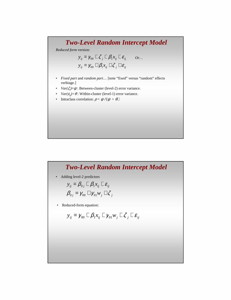
Two-Level Random Intercept ModelReduced formversion:

ijjijij

ijijjij

xy

xy

εζβγεβζγ

+++=

+++=

100

100 Or…

• Fixed partand random part… [note “fixed” versus “random” effects verbiage.]

• Var(ζi)=ψ : Between-cluster (level-2) error variance.

• Var(εij)=θ : Within-cluster (level-1) error variance.

• Intraclass correlation: ρ = ψ / (ψ + θ)

Two-Level Random Intercept Model• Adding level-2 predictors

jjj

ijijjij

w

xy

ζγγβεββ++=

++=

01000

10

• Reduced-form equation:

ijjjijij wxy εζγβγ ++++= 01100

GLS Estimation of Linear Random Intercept Model

ijjijij xy εζβγ +++= 100

• Again, note that we’re dealing with fixed β. • Can be estimated via GLS and ML; both yield similar results.• Foundation: GLS estimates of β1 are a weighted average of the

pooled and within estimates of β1.– Partial pooling of coefficients.

GLS Estimation of Linear Random Intercept Model

• Within, between, OLS, and GLS estimates:

ψθθω

ωωβ

β

β

β

n

BWBW

BWBW

BB

WW

xyxyxxxxGLS

xyxyxxxxOLS

xyxxB

xyxxW

+=

++=

++=

=

=

−

−

−

−

)()(

)()(1

1

1

1

• n = cluster size; this equation assumes balanced structure (i.e., equal cluster sizes), though you can relax this for unbalanced structure.

• If ω = 0, βGLS reduces to βW.

• If ω = 1, βGLS reduces to βOLS.

• As cluster size increases, βGLSbecomes more similar to βW.

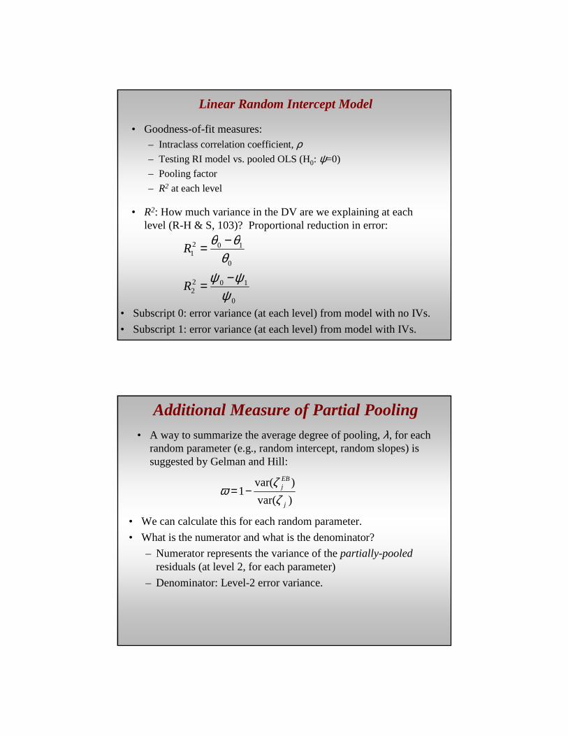
Linear Random Intercept Model

• Goodness-of-fit measures:– Intraclass correlation coefficient, ρ– Testing RI model vs. pooled OLS (H0: ψ=0)

– Pooling factor

– R2 at each level

• R2: How much variance in the DV are we explaining at each level (R-H & S, 103)? Proportional reduction in error:

0

1022

0

1021

ψψψ

θθθ

−=

−=

R

R

• Subscript 0: error variance (at each level) from model with no IVs.

• Subscript 1: error variance (at each level) from model with IVs.

Additional Measure of Partial Pooling• A way to summarize the average degree of pooling, λ, for each

random parameter (e.g., random intercept, random slopes) is suggested by Gelman and Hill:

)var(

)var(1

j

EBj

ζζ

ω −=

• We can calculate this for each random parameter.

• What is the numerator and what is the denominator?

– Numerator represents the variance of the partially-pooledresiduals (at level 2, for each parameter)

– Denominator: Level-2 error variance.

Interpretation of Effects for All Approaches

• How do we interpret effects from each approach?

• What do the pooled and RI approaches assume about the within- and between-cluster effects?

WithinWithin--Cluster v. BetweenCluster v. Between--Cluster VariationCluster VariationStudent School Y X1 X2 X3 X4

1 1 54 2 32 1 44

2 1 64 4 25 1 44

3 1 87 9 45 1 44

4 2 24 4 44 0 36

5 2 98 7 32 0 36

6 2 65 6 22 0 36

7 3 45 9 19 0 22

8 3 32 5 15 0 22

9 3 37 2 25 0 22

10 4 84 7 30 1 45

11 4 45 4 38 1 45

12 4 65 3 36 1 45

13 5 21 8 41 1 18

14 5 65 6 22 1 18

15 5 98 1 18 1 18

Considerations for the FE (Within) Estimator• It’s an easy way to account for unobserved heterogeneity in the

response.

• Since the ζj are treated as fixed, instead of random, the potential for endogeneity between X and ζj (the controversial assumption) is eliminated.

• Consistent as N and J infinity.

• More appropriate for inferring to clusters in sample only?

Issues:

• Overall efficiency loss by eliminating between group variation.

• FE cannot produce estimates for variables that are constant within clusters (level-2 vars; time-invariant in panel and TSCS data).

• Difficult to generate precise estimates for the effects of variables that contain small within-cluster variation.– This is a problem with the data, though, and not FE, per se.

Considerations for the Random Intercept Model• More efficient than FE (minimum variance property)

• One can include variables that are constant within clusters (unlike the within estimator).

• Appropriate when inferring to populationof clusters?

• Issue: Correlation between random effect and X at level 1.

IV. Cluster Confounding

Controversial Assumption in the RI Model

jj

ijijjij xy

0000

10

ζγβεββ

+=

++=

0),( 0 =ijj xCov ζ

[Level-1 equation]

[Level-2 equation]

Controversial Assumption

• Issue: We need an accurate estimate of β1. Note that this is fixed, so that βGLS, βW, βB

are all estimates of the same parameter, β.

• Note that βGLS (and OLS) assumes that the between and within effects are the same (i.e., β). – Remember that xij varies both within and between clusters.

• But….the between effect could differ from the within effect for a variety of reasons.

• “Cluster confounding”; due to omitted variable(s) at level-2 (which are related to xij), β1 could be confounded by conflicting between and within effects.

• Cluster confounding occurs when we’ve assumed the within and between effects are the same (by estimating a pooled or partially-pooled β), but they’re actually different.– Think about what it would take to eliminate the controversial assumption in the model

above? Also, connection to ecological fallacy.

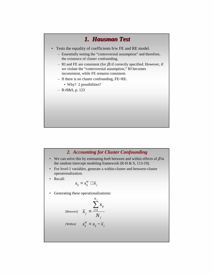
1. 1. HausmanHausman TestTest• Tests the equality of coefficients b/w FE and RE model.

– Essentially testing the “controversial assumption”and therefore, the existence of cluster confounding.

– RI and FE are consistent (for β) if correctly specified. However, if we violate the “controversial assumption,” RI becomes inconsistent, while FE remains consistent.

– If there is no cluster confounding, FE=RE.

• Why? 2 possibilities?

– R-H&S, p. 123

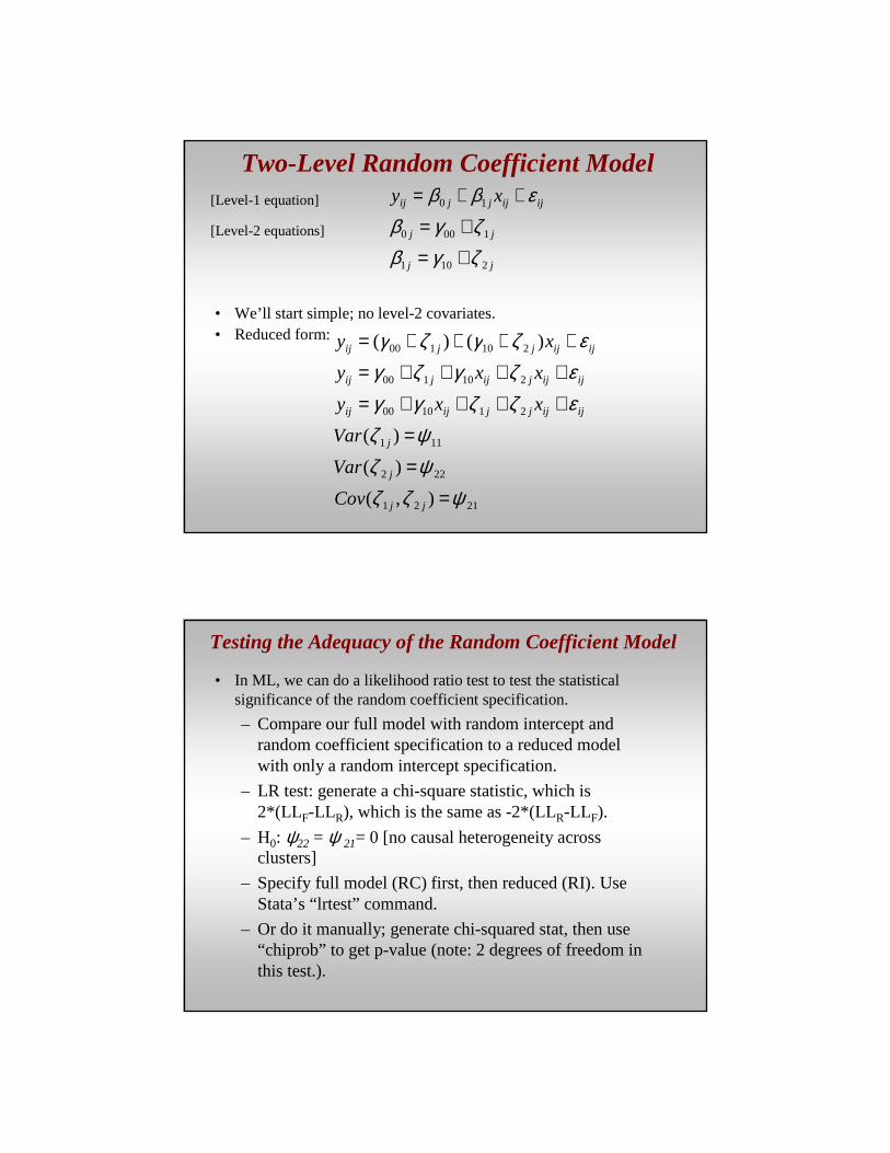
2. Accounting for Cluster Confounding• We can solve this by estimating bothbetween and within effects of β in

the random intercept modeling framework (R-H & S, 113-19).

• For level-1 variables, generate a within-cluster and between-cluster operationalization.

• Recall:

j

N

iij

j N

xx

j

∑== 1

jWijij xxx +=

• Generating these operationalizations:

[Between]

[Within]jij

Wij xxx −=

2. Accounting for Cluster Confounding• Estimate both the within and between-cluster effects of xij

• Method 1:

ijjjBW

ijW

ij xxy εζβββ ++++= 0

• Method 2 (identical model, different interpretation):

ijjjijW

ij xxy εζδββ ++++= 0

• What is the correlation now between the within-cluster xij andζj?

• Can perform Hausman-like test for equality of between and within estimates. δ represents the differencebetween with the within- and between-cluster effects.

• Importance: Highlights consequences for the models assuming within- and between-cluster effects are equal.

V. Panel / Time-Series Cross-Sectional Data

Panel / TimePanel / Time--Series CrossSeries Cross--Sectional DataSectional Datai j t Y X1 X2 X3 X4

1 1 1 54 2 32 1 44

2 1 2 64 4 25 1 44

3 1 3 87 9 45 1 44

4 2 1 24 4 44 0 36

5 2 2 98 7 32 0 36

6 2 3 65 6 22 0 36

7 3 1 45 9 19 0 22

8 3 2 32 5 15 0 22

9 3 3 37 2 25 0 22

10 4 1 84 7 30 1 45

11 4 2 45 4 38 1 45

12 4 3 65 3 36 1 45

13 5 1 21 8 41 1 18

14 5 2 65 6 22 1 18

15 5 3 98 1 18 1 18

Issues in TSCS Data• Unobserved heterogeneity

• Pooling

• Temporal dependence

• Efficiency – standard errors– Panel heteroskedasticity (panels have different error variance)

– Contemporaneous error correlation (errors related across countries for given years)

– Serial correlation

Beck and Katz 1995• Recommended using OLS with panel-corrected standard errors

(PCSEs)– Serial correlation should be eliminated before estimation.

– Adjusts SEs for panel heterosk. and contemporaneous correlation.

• Like robust standard errors in OLS for cross-sectional data.var(b)=(X’X) -1 (X’ Ω Ω Ω Ω X)(X’X) -1

– Ω is the same as in GLS.

– The larger T is, the better the PCSEs are.

– In Stata, “xtpcse”

• Article did not place emphasis on UH, just standard error correction; they also suggest AR-1 correction.

• What kind of an approach is this?

Beck and Katz 1996• Now widely accepted in political science: Beck and Katz

(1996); FE with lagged DV and PCSEs.

• Same issues apply to TSCS/panel data that we have talked about– Modeling approaches along pooling spectrum

– Cluster confounding

• Primary difference is dynamics.

VI. Random Coefficient Model

Two-Level Random Coefficient Model• Motivation for random coefficient model: Causal

heterogeneity.

Two-Level Random Coefficient Model

• We’ll start simple; no level-2 covariates.• Reduced form:

jj

jj

ijijjjij xy

2101

1000

10

ζγβζγβ

εββ

+=

+=

++=[Level-1 equation]

[Level-2 equations]

2121

222

111

211000

210100

210100

),(

)(

)(

)()(

ψζζψζψζ

εζζγγεζγζγ

εζγζγ

=

=

=

++++=

++++=

++++=

jj

j

j

ijijjjijij

ijijjijjij

ijijjjij

Cov

Var

Var

xxy

xxy

xy

Testing the Adequacy of the Random Coefficient Model

• In ML, we can do a likelihood ratio test to test the statisticalsignificance of the random coefficient specification.

– Compare our full model with random intercept and random coefficient specification to a reduced model with only a random intercept specification.

– LR test: generate a chi-square statistic, which is 2*(LL F-LLR), which is the same as -2*(LLR-LLF).

– H0: ψ22 = ψ 21= 0 [no causal heterogeneity across clusters]

– Specify full model (RC) first, then reduced (RI). Use Stata’s “lrtest” command.

– Or do it manually; generate chi-squared stat, then use “chiprob” to get p-value (note: 2 degrees of freedom in this test.).

Random Coefficient Modelijijjjij xy εζγζγ ++++= )()( 210100

• Think about what this means: – The random effect for the intercept represents a cluster’s deviation from

the “mean intercept.” [more specifically…..]– The random effect for the slope represents a cluster’s deviation from the

“mean slope.”

• Mean-centering: The random intercept actually represents the cluster average when x=0. To make substantive interpretations of the random intercept part, we can mean-center the x’s at level 1. • Then, the intercept represents the average cluster level of the DV,

since it’s for a typical value of x.

Random Coefficient Model• Generating empirical Bayes residuals at level 2 for the slope

and intercept.

• Using these to calculate partially-pooled slopes and intercepts.

Random Coefficient Model with Cross-Level Interactions

jjj

jjj

ijijjjij

w

w

xy

211101

101000

10

ζγγβζγγβεββ

++=

++=

++=[Level-1 equation]

[Level-2 equations]

• Causal heterogeneity, in addition to heterogeneity in the response.• Level-2 error components are distributed multivariate normal, with means

of zero and estimable variances and covariance.

Random Coefficient Model with Cross-Level InteractionsReduced form

ijjijjijjijjij

ijijjijjijjjij

ijijjjjjij

xxwxwy

xxwxwy

xwwy

εζζγγγγεζγγζγγ

εζγγζγγ

++++++=

++++++=

++++++=

1211100100

2111010100

2111010100 )()(

Cross-level interaction Composite

error term

• Mean centering: importance for understanding constituent effects when there are interactions

– No mean centering

– “Grand mean” centering

– Cluster mean centering (like operationalizing within and between-cluster versions of a level-1 variable.

Estimation

• Note for linear models, differences in estimation procedures is not a huge deal; it’s a bigger deal for nonlinear models.

• Estimation techniques: – GLS

– Maximum likelihood

– Restricted ML (REML)

• All three are asymptotically equivalent

Maximum Likelihood Estimation• Conditional distribution of the response (conditional on the

random effects):

where ζ ~ MVN(0, Σ) );,|()1( θζXYg

∫ ∏=

=jn

i

dXYghXYf1

)1()2( );,|()();|( ζθζζθ

• Goal: Obtain the unconditional (marginal) distribution of the response for each cluster j by integrating out the random effects:

• Marginal likelihood:

∏=

=J

j

XYfL1

)2( );|( θ

• Or:

∏ ∫ ∏= =

=J

j

n

i

j

dXYghL1 1

)1( );,|()( ζθζζ

Maximum Likelihood Estimation• For linear model: there’s a closed form solution to integral.

– For nonlinear models, integral is approximated using quadrature

• Use EM algorithm to maximize the likelihood– Mutual dependence of estimates for fixed effects and variance

components

– Iterative procedure; alternate between “expectation” and “maximization” steps

Differences b/w ML and REML• Differences are minor, and primarily center on calculating the

variance components.

• In REML, likelihood function not directly applied to the response, Y. Instead, the restricted likelihood is the full likelihood with the variance components only and the fixed effects swept out. Fixed effects (coefficients) estimated in second step.

• REML accounts for the loss of degrees of freedom due to estimation of parameters; generates unbiased estimates of the variance components.

• ML estimates do not account for this loss of df, and they are consistent. There’ll be a downward bias of ψ in small samples (particularly small number of clusters).

• This is analogous to OLS versus ML estimates of error variance in linear regression.

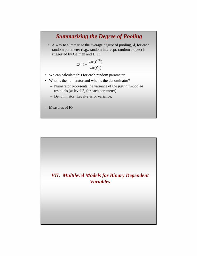
Summarizing the Degree of Pooling• A way to summarize the average degree of pooling, λ, for each

random parameter (e.g., random intercept, random slopes) is suggested by Gelman and Hill:

)var(

)var(1

j

EBj

ζζ

ω −=

• We can calculate this for each random parameter.

• What is the numerator and what is the denominator?

– Numerator represents the variance of the partially-pooledresiduals (at level 2, for each parameter)

– Denominator: Level-2 error variance.

– Measures of R2

VII. Multilevel Models for Binary Dependent Variables

Binary Responses: GLM Specification• Hierarchical generalized linear models (HGLM):

1. Specify the sampling model for the dependent variable.

2. Specify link function (first, conditional expectation of response; then, the link is the inverse of that)

3. Specify structural model; model link as a linear function of independent variables.

• For linear models, we don’t really need to think in a GLM format:

Yi = b0+b1Xi+ei

• But we could: Normal sampling model, identity link [µi=E(Yi | Xi)=x’β]

GLM Specification• Utility of HGLM: For nonlinear models.

• Example for binary DVs1. Bernoulli sampling model

2. Logit link:

a. Conditional expectation of response:

E(Yi | Xi) = µi = Pr(Yi=1 | Xi) = exp(x’β) / [1+ exp(x’β)]b. Link is the inverse of µi

ηi=log[µi / (1 –µi)] [log-odds]

3. Structural model: write ηi as a linear function of level-1

Estimation• See handout

• gllamm or xtmelogit (uses quadrature)

Estimating Multilevel Models with Binary Responses in Stata

• xtlogit and xtprobit : random intercept models only (default is adaptive quadrature, 12 points)

• xtmelogit: RI and RC logit model (default is adaptive quadrature, 7 points)

• gllamm: add-on package to Stata (created by Rabe-Hesketh and Skrondal); estimates RI and RC models for all types of DVs(continuous, binary, ordinal, count, duration, nominal); uses quadrature and adaptive quadrature.– To install, type (in Stata): ssc install gllamm

• See handout on gllamm.

• Using good start values and increasing number of quadrature points.

Generating Quantities of Interest• In gllamm, use the “gllapred” command (after specifying a

gllamm model)

• To retrieve empirical Bayes residuals:gllapred eb, u

• For an RI model, this will generate two variables: ebm1 and ebs1. – ebm1 is the empirical Bayes residuals (like what we get with

“reffects” in the canned xtmixed and xtmelogit). – ebs1 is the s.e. of the EB residuals

• For an RC model, the command will generate four variables: ebm1, ebs1, ebm2, and ebs2. “1” is for random intercept, “2”is for random slope.

Probabilities in Binary Response Models• Two different brands of predicted probabilities:

– Cluster-specific probabilities• Takes into account the clustering, hierarchical structure in the data.

• RI and RC models fit cluster specific probabilities: Pr(Y=1 | ζ, x)

– Marginal, or “population-averaged,” probabilities• Marginal with respect to the random effects; plain-vanilla logit and

probit produces marginal, PA probabilities: Pr(Y=1 | x). They don’t depend on ζ, because we’re not modeling it.

• To generate marginal probabilities from an RI or RC model, need to integrate out ζ, as on p. 254 (eq. 6.7).

• See page 255 in RH&S; difference between cluster-specific and marginal probabilities.

Probabilities in Binary Response Models• Generating cluster-specific probabilitiesafter running a

gllamm model; use the “gllapred” command.

gllapred cs_prob, mu

• This will generate a predicted prob for observations in the sample, using the cluster’s particular ζ. See pp. 269-70.

• Generating marginal, or PA, probabilities after running a gllamm model:

gllapred marg_prob, mu marginal