multigrid methods for differential … · multigrid methods for differential equations with highly...
TRANSCRIPT

85
MULTIGRID METHODS FOR DIFFERENTIAL
EQUATIONS WITH HIGHLY OSCILLATORYCOEFFICIENTS,
Bjorn Engquist Erding Luo
Dept. of Math., UCLA, CA 90024
SUMMARY
New coarse grid multigrid operators for problems with highly oscillatory coefficients are
developed. These types of operators are necessary when the characters of the differential
equations on coarser grids or longer wavelengths are different from that on the fine grid.
Elliptic problems for composite materials and different classes of hyperbolic problems are
practical examples.
The new coarse grid operators can be constructed directly based on the homogenized
differential operators or hierarchally computed from the finest grid. Convergence analysis
based on the homogenization theory is given for elliptic problems with periodic coefficients
and some hyperbolic problems. These are classes of equations for which there exists a
fairly complete theory for the interaction between shorter and longer wavelengths in the
problems. Numerical examples are presented.
INTRODUCTION
Multigrid methods are usually not so effective when applied to problems for which the
standard coarse grid operators have significantly different properties from those of the fine
grid operators [1,3,7-9,11-12]. In some of these problems the coarse grid operators should
be constructed based on other principles than just simple restriction from the finest grid.
Elliptic and parabolic equations with strongly variable coefficients and some hyperbolic
equations are such problems. One feature in these problems is that the smallest eigenvalues
*This work was partially supported by grants from NSF: DMS 91-03104, DARPA: ONR N00014-92-J-1890, and ARO: ARM DAAL03-91-G0162.
PIt_CtiI'_NG P.'_:_ DLAr_K NOT FN_N_DPAGE_ INTENTIONALLYBLANM'r
175
https://ntrs.nasa.gov/search.jsp?R=19940019212 2018-08-17T23:20:17+00:00Z

do not correspond to very smooth eigenfunctions. It is thus not easy to represent these
eigenfunctions of the coarser grids.
We shall investigate elliptic equations with highly oscillatory coefficients,
0 0 x)_j --_xjaj(x)-_xjU¢(X ) = f(x), aZ(x ) ----aj(x,e
(l)
with aj(x,y) strictly positive, continuous and 1-periodic in y. This is one class of the
problems discussed above for which there exists a fairly complete analytic theory such that
a rigorous treatment is possible. This homogenization theory describes the dependence of
the lal'ge scale features in the solutions on the smaller scales in the coefficients [2,11]. We
shall consider model problems but there are also important practical applications of these
equations in the study of elasticity and heat conduction for composite materials.
In this paper we analyse the convergence of multigrid methods for equation (1) by
introducing new coarse grid operators, based on local or global homogenized forms of the
equation. We consider only two level multigrid methods. For full multigrid or with more
general coefficients the homogenized operator can be numerically calculated from the finer
grids based on local solution of the so called cell problem [2].
In a number of numerical tests we compare the convergence rate for different choices of
parameter and coarse grid operators applied to a two dimensional elliptic model problem.
The convergence rate is also analyzed theoretically for a one dimensional problem.
If, for example, the oscillatory coefficient is replaced by its average, the direct estimate
for multigrid convergence rate is not asymptotically better than just using the damped
Jacobi smoothing operator. The homogenized coefficient reduces the number of smoothing
operations from O(h -2) to O( h-l°/r log h ). When h/e belongs to the set of Diophantine
numbers [4], ergodic mixing improves the estimate to O(h -6Is log h). The step size is h and
the wave length in the oscillating coefficient e.
These results carry over to some but not all hyperbolic problems. A numerical study
of using hyperbolic time stepping with multigrid inorder to compute a steady state gives
similar results to the elliptic case.
TWO DIMENSIONAL ELLIPTIC PROBLEMS
Elliptic problems on the form (1) will be considered,
-- V .ae(x,y)Vue = f(x,y), (x,y) e a = [0,1] x [0,11, (2)
subject to Dirichlet boundary condition U_lon = O. The function a_(x,y) = a(x/e,y/e) is
176
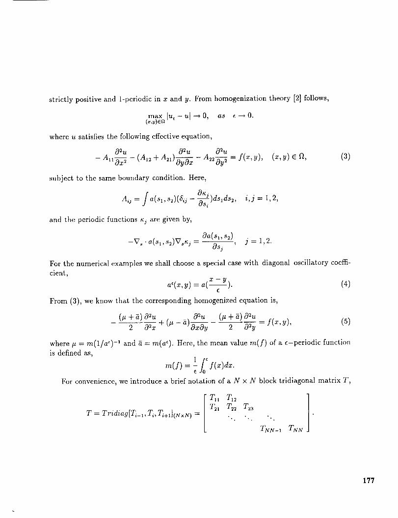
strictly positive and 1-periodicin x and Y. From homogenization theory [2] follows,
max ]ue -- ul ---* O, as e ----_O.
where u satisfies the following effective equation,
O_u 02u A 02u- All_x 2 - (A12 + A21)OyOx 22-_y2 = f(x,y), (z,y) e _,
subject to the same boundary condition. Here,
O_J)dsld%, i,j = 1,2,Osi
I"
Aij = j a(sl,%)(6ij
and the periodic functions _j are given by,
-Vs" a(sl,s2)Vs_j = 0sj , j = 1,2.
(3)
For the numerical examples we shall choose a special case with diagonal oscillatory coeffi-
cient,
a_(x, y)= _(5__). (4)
From (3), we know that the corresponding homogenized equation is,
(# + _) 02u O_u (# + a) 02u _ f(x,y), (5)2 02x + (# - a)OxOy 2 02y
where # = m(1/aO-' and a = re(a<). Here, the mean value re(f) of a e-periodic function
is defined as,
1 f(x)dx.m(f) = e
For convenience, we introduce a brief notation of a N x N block tridiagonal matrix T,
TI, T12
23
TNN-1 TNN
T = Tridiag[Ti_l, Ti, Ti+ll(NxN ) =
177

Numerical Algorithm
The discretization of (2) combined with (4) is
- D_ ahj D: u}j - DY+bhjD_ uhj = fh. (6)
whereab =a_(xi,_ --ih _yj), bh.=a_(xi--yj+-_),,, i,j=O,...,N. D+ andD_ areforward1 denotes the grid size. Using vectorand backward divided differences, respectively; h =
notation, we can rewrite (6) as
L ,h G,h = G,h
where1
L¢,h = fi Tridiag[B h_ 1' Ah, Bjh](N-1)x(N-l) (7)
Ah = Tridiag[-ah u'ah-lJ + ah + bh + bh ha - ij-l' --aij](N-1)x(N-1)
B h is a diagonial matrix, denoted by B h = Diag[--bhj](N_l)x(N_l) and3 3
, ""., "'',UN_IN_ 1)UG h (Uhl, U2hl ' h h /t2hN_ 1 h T" " " ?J'N-11 _ _IN-I'
h= .... , - • •, f_r_lN_l)re,h (fhl, fhl, " ., f_r_ll ' ,fhlN_l,fhN_ 1 h T
For simplicity, we only consider the two-grld method. Denote the full iteration operator of
this method by M. It is defined by,
M = S'r(I h -1 H "1-- I_,L H I_ L,,h)S , (8)
where the restriction and interpolation operators are given, as denoted below, by the weight-
ing restriction and bilinear interpolation operators, respectively,
11121[I I1 1 2 ] h
I_'=_-_ 2 4 2 , I_=_ 2 4 2 .1 2 1 h 1 2 1 H
The smoothing iteration operator S is based on the damped Jacobi iteration,
S = I-wh2L,,h . (9)
The coarse grid operators L H is one of the following operators:
178

Global Homogenized operator." which is the discretized form of (5)
-0.5(tL + a)D_+D_uij + (# - a)DoD_uij - 0.5(# + gt)Du+D[uij = fij.
Written in matrix form,
1
L H = -_Tridiag[BH_I,AH, BjH]@_I)×(__I),(lO)
where
A H = Tridiag[ # + _ + a, 2 ' + a), 2
a -- _ _ "-1- a a -- _](___I)x(N_I) "/3( I Tridiag[J 4 ' 2 ' 4
Local Homogenized operator: L H has the same form as (10), except the entries for A_ r, BH3
coming from the local discretized values of a¢(x - y),
1
Lu = -_ Tridiag[Bj_l, AH, BjH](-__l)x(-_-l),(11)
where
with
AH_ = Tridiag[--aHlj,aHlj + a g,, + bHij-, + bHij' --aH]' N--')X @--1)',J_' 7
BU =, Tridiag[-ciH_,,-bH, j, ciH] (_ -1)x (q-l) '
b h, qL bhj_ 1 q- 2(_(bhj,bh_l ) ah.. q- ah 1 -1- 2_(ahj, aLlj) [z --bH. = ,3 a H= 'J cH=-': 4 ' 'J 4 ' ' 2
5(Cl,C2) is defined to beCl -t- c2 "
Reduced Local Homogenized operator: L H has the same form as in (11), except here we ig-
nore the cross term D O_D 0.y That means BH_ is a diagonM matrix, BH: = Diag[-bH]@_l)×(___l),
1= [j_I,A_,B_]@_,)x(_}_I)LH -i_Tridiag B H
(12)
Sampling operator: L_, H has the exact form as Le,h, but values aij , b0 are defined on the
coarse grids,
LH = L_,H (13)
179

Variational operator:
L H = IhHL¢,h Ih (14)
Numerical Results
In practice, it is not always easy to calculate the spectral radius p(M). Therefore, we
study the mean rate [14] of convergence under different coarse grid operators L H. The
mean rate of convergence is defined by
p = ( IIL ,hu - hlth (15)
where i is the smallest integer satisfying []L,,hu _ - fhIIh <-- 1 X 10 -6.
In Figure 1, a_(x-y) = 2.1 + 2sin(2:r(x-y)/¢). We plot p defined by (15) as a function
of 3' by taking e = v_h, and w in (9) is 0.095.
1
0.8
0.6
0.4
0.2
0
0.8
0.6
0.4
0.2
0
0.8
0.6
0.4
0.2
0
0 5 10 15 20 25 0 5 10 15 20
(1.1) N=16 (1.2) N=32
_ _"_ +++ ++
_ ,- +++++++++++++.
25
0.8
0.6
0.4
0.2
0
==============================
0 5 10 15 20 25 0 5 10 15 20 25
(1.3) N=64 (1.4) N=128
Figure 1: p as a function of 3'. Dotted line is for (10), solid line for (11), dashed line for (13), and dashdot for
(12), + for (14). (1A)-(1.4) are for different number of grid points N.
180

It is clear that the coarse grid operators derived from the homogenized forms (10)
and (11) are superior. The effect is more pronounced for large "7 when the eigenspace
corresponding to large eigenvalues of L_,h is essentially eliminated. For the practical low
7 case, a study of the impact of the choices of I/_ and I H is needed. In this paper we are
concentrating on the asymptotic behavior (large 7). Different I_ and I_ operators are
briefly discussed for the one-dimensional problem.
In Figure 2, we plot p as a function of the variable a, where LH(a ) comes from the
discretized operator --ariD ":D x + a(# -a)D_Dg ,,H r_Y nY v_h.0 + - - _ijL'+'-'-, w = 0.095 and e =
1
o.9
om
o.8
os
o4
o.s_- 0,2
Figure 2: p as a function of a. Here N = 64 and "/= 12. "*" denote p under the different choice of NorrnM
and Local Homogenized coarse grid operator, respectively.
From Figure 2, we get further evidence of the importance of using the correct homoge-
nized operator. Techniques based on one-dimensional analysis does not contain the mixed
derivative term [1].
In order to isolate the influence of the coarse grid approximation we have kept the
smoothing operator fixed. It obviously also affects the performance. If we use Gauss Seidel
iteration method in (9), the convergence rate can be improved. In Table 1, we test the
same coefficient a_(x-y) = 2.1 +2sin(27r(x-y)/e). Taking N = 128, e = v/2h, we compare
the convergence rate by choosing damped Jacobi iteration and Gauss Seidel iteration.
5 6 7 8 9 10 11 12
Jacobi .5929 .5519 .5173 .4863 .4579 .4349 .4140 .3950
G-S .4545 .4221 .3922 .3703 ....13491 .3304 .3158 .3008
Table 1: Spectral radius, two dimensional case
181

ONE DIMENSIONAL PROBLEMS
The one dimensional equation is useful as a model for which a more complete mathe-
matical analysis is possible.
Consider the following one-dimensional elliptic boundary value problem with a periodic
oscillatory coefficient, : _ _ ....
d _ du__a (x)-dT = 1, 0 < x < 1, _(0) = _(1)=0, (16)
where a_(x) = a(_) and satisfies the same assumption as above. As ¢ _ 0, u_ converges
strongly in Loo to the solution u of the homogenized equation,
d2u
- _dx_ 1, 0 < x < 1, _ ._(1/a9 -1. (17)
Subject to the boundary conditions ¢(0) = ¢(1) = 0.
Numerical Algorithm
Let the difference approximation of (16) be of the form:
_a_(x._l)(uh _uh)+aqx " _(u h h3-1- 7 _ j+l x 3-7J_ 3- t/J -1) = 1,
In matrix form, (18) can be written as=
where
j = I,..-,N- 1 (18)
L_,hu h= l, u h = (uhl ...,uhN_,)T
i
L_,h = -_Tridiag[-ai_l,ai_l + ai,ai+l](N_l)×(N_ 0 (19)
with aj=a_(xj-_).
We first consider a two-grid method by applying standard restriction, standard inter-
polation operators and Jacobi smoothing iteration.
The coarse grid operator LH will be one of the following:
Homogenized operator:
A veraged operator:
m(1/a_) -1
L H -- H_ Tridiag[-1,2,-1](___)x@__) (20)
LH - m(a_)Tridiag[-1,2,-1](q_l)×(____) (21)H 2
182

Sampling operator: L¢, H has the exact form as L_,h, but only every second aj value is used,
L H = L¢, H (22)
Variational operator:
L. = (23)
Convergence Theory
The theorem below on the convergence rate is too pessimistic in the number of smooth-
ing iterations necessary. However, the analysis still gives insight into the convergence
process and the role of homogenization. With LH replaced by averaging (21) the same
analysis results in 7 = O(h-2) which means that multigird does not improve the rate of
convergence over just using Jacobi iterations. This follows from the effect of the oscillations
on the lower eigenmodes. It should also be noticed that in the case (ii), the solution of L_, h
is much closer to those of LH, see [11].
Theorem 1 Let M be defined as in (8), with L H defined by (11). There exists a constant
C such that,
p(M) < Po < 1,
when either one of the following conditions is satisfied:
(i) _/ >_ Ch-l-a/rlnh
(ii) the ratio of h to e belongs to the set of Diaphantine number, and 7 >- Ch-l-1/Slnh.
For details of the proof, see [10]. An outline is as follows. Separate the complete eigenspace
of L¢,h into two orthogonal subspaces, the space of low eigenmodes and that of high eigen-
modes. After several Jacobi smoothing iterations in the fine grid level, the high eigenmodes
of the error are reduced, and only the low eigenmodes are left. Combining eigenvalue analy-
sis with homogenization theory [11], one may realize that the low eigenmodes of the original
discrete operator are close to those of the corresponding homogenized operator. We then
approximate them by the corresponding homogenized eigenmodes and correct these in the
coarse grid level.
183

Numerical Results
In Figure 3.1 and Figure 3.2, a_(x) = 2.1 + 2 sin(27rx/e). We plot the analogous graph
to Figure 1. Here e = v/2h and _ in (9) is 0.1829. In Figure 3.3 and Figure 3.4, a_(x) =
2.1 + 2sin(2_rx/c + _/4). Here e = 4h and w = 0.1585.
1.4
1.2
1
0.8
0.6
0.,4
0.2
0 0
1 \ 1.4-
1.2
o._
O.q5
O°4-
Ct.2
1..4
1.2
1
0.6
0.6
0..4-
0.2
O o
\\\ \
\ \,_ \ "\
-- _'_'--_ --_ Y- --2 L'C L--
\,
lo 20 10 20
(3.1) N--lfi (3.2) N=1211
_t°4
1.2
o._
O_
O_
_o2
O_
i\.\.
i\ \
t
10 20 10 20
(3.3) N=I6 (3.4) N=128
Figure 3: p as a function of_¢. Dotted line is for (20), solid line for (21), dashed line for (22), and dashdot for
(23). (3.1)-(3.4) are for different number grid points N.
In Figure 4, with the assumptions in Figure 3.3-3.4, we plot a_(x) and the approximation
of (18) under the choices of coemcients in Figure 3.
1-4-(_
4.S
4
3
2.5
2
O._
O o
0.3_
0.3
0.2_
0.2
0.1:5
0.1
O°O_
O o20
(4ol) N_32 (-4-.2) S • tit
2O 3O
Figure 4: (4.1) and (4.2)axe the graphs for a'(z), where * are the discretized values. (4.2) is the solution.
Dashed line is for (17). Dashdot line is for -m(a')un m 1 and line with circles is for (18).
184

In Figure 5, we plot p as a function of the variable a, where L H = aA H. In (5.1),
a*(z) = 2.1 + 2sin(2_z/e), w = 0.1829 and e = v_h; In (5.2), a_(x) = 20.1 if x/e -Ix/el e(0.7,0.9); otherwise, O.1, w = 0.0373 and e = 4h.
z
0.9
O.m
O.95
O.9
O.B5
O.a
_t nR4-_
] O _ :2,.It "I
Figure 5: p as a function of c_. The homogenized value ah = m(1/ae) -1 and the arithmetic value av = m(a e)
are given. Here "y = 10 and N = 256.
In Figure 6, we present the convergence u_ + u, as e + 0 by giving the numerical solutions
of (16) and (17). Recall that our goal is to solve the oscillatory problem and to use the
homogenized operator only for the coarse grids.
ilj
,,' \
t
o _ lt:)o
,(_. l)
O. lt8 -"
O. 16 .,
O. 14 /
O. 12 /
O.l
O.OS /£
O._ ?'
0.0.4 '
O.O2 ,;
O
<6.2)
Figure 6: Solid lines are the approximations for (18), dashed lines are the solutions for (17), respectively,
when e = 0.2 in (6.1) _nd _ = 0.1 in (6.2). Here N = 500.
185

HYPERBOLIC PROBLEMS
Time evolution of a hyperbolic differential equation canbeusedfor steadystate computa-tions. This is common in computational fluid dynamics, [6]. In multigrid this meansthathyperbolic timestepping replacesthe smoothing step. There are fundamental differenceswith standard multigrid for elliptic problemsbut someof our earlier discussionscarry over
to the hyperbolic case. The dissipative mechanisms for hyperbolic problems are mainly the
boundary conditions. Consider using the model problem,
02u, 0 , Ou,Ot 2 Ox a (z)--_x = f(z), 0 < x_< 1 (24)
as the smoothing equation in multigrid for the numerical solution of (16), subject to the
boundary conditions0_t(1)
ut(o) = o, Ox -0. (25)
The equation (24) must have boundary conditions which are dissipative but reduce to (25)
at steady state, see [5],
u_(O,t) = O, Ou_(1,t) r-----Ou_(1,t)Ot + _/a_(z) -_x - O. (26)
The initial condition should support the transport of the residual to the dissipative
boundary x = 1,
u_(x,_)= u0(x) given,
Note that the initial condition approximates the transport equation ut + v/auz = 0. The
difference approximation of (24) needs a low level of numerical dissipation.
The homogenization theory of [2] is also valid for equation of the type (24). A numerical
indication is seen in Figure 7.
The positive effect of muItigrid on the convergence rate does not carry ever to problems
for which the steady state is hyperbolic or contains hyperbolic components. If,
Out Out Ou_
0_ + %7 + Z-b7 =°
is used for the equation,
U_
Otl t O_l e
+ _-N:v= o,
is 1 -periodic in
186

The coarse grid operator must resolve all scales of a _ to required accuracy in order to
produce multigrid speed up. More on this phenomena will be reported elsewhere.
Numerical Results
In Figure 7, take 50 smoothing steps. Coefficient a(x/e) is the same as in Figure 1.
8O
60
40
20
0
3000
2000
1000
00 20 40 60 I0 15 20
(7.1) (7.2)
80 80
60 60
40 40
20 20
0 00 20 40 60 0 20 40 60
(7.3) (7.4)
Figure 7: (7.1) Solutions: Solid line is the solution of steady state; Dashed line for homogenized solution;
Dashed dot line for average solution. (7.2) Residue as function of two level multigrid cycles. (7.3) Approximate
solutions after each two level cycle. (7.4) Approximate solutions for time evolution equation.
CONCLUSION
Elliptic equations and some hyperbolic equations with highly oscillatory coefficients
have been studied. We have shown that the homogenized form of the equations are very
useful in the design of coarse grid operators for multigrid.
187

The evidence is from a sequence of numerical examples with strongly variable coefficients
and to some extent from theoretical analysis. The result is clear in the asymptotic regime
of many smoothing iterations.
The impact on the coarse grid operator from the numerical truncation error and the
interpolation operator needs to be asessed in order to improve the performance in the
regime of very few smoothing iterations per cycle.
References
[1] Alcouffe, R.E.; Brandt, A.; Dendy, J.E.; and Painter, J.W.: The Multi-Grid Method
for the Diffusion Equation with Strongly Discontinuous Coefficients. SIAM J. Sci.
Stat. Comput., vol. 2, no. 4, 1981, pp. 430-454.
[2] Bensonssan, A.; Lions, J.L.; and Papanicolaou, G.: Asymptotic Analysis for Periodic
Structure, North-Holland, Amsterdam, 1987.
[3]
[4]
Brandt, A: Multi-level Adaptive Solutions to Boundary-Value Problems. Mathematics
of Comput., vol. 31, no. 138, 1981, pp. 333-390.
Engquist, B.: Computation of Oscillatory Solutions for Partial Differential Equations.
Lecture Notes 1270. Springer Verlag, 1989, pp. 10-22.
[5] Engquist, B.; and Halpern, L.: Far Field Boundary Conditions For Computation Over
Long Time. Applied Numerical Mathematics, no. 4, 1988, pp. 21-45.
[6] Jameson, A.: Solution of the Euler Equations for Two-Dimensional Transonic Flow
by a Multigrid Method. Appl. Math. comput., no. 13, 1983, pp. 327-355.
[7] Hackbusch, W.; and Trottenburg, U., eds.: MuItigrid Methods. Lecture notes in math-
ematics 960. Springer Verlag, 1981.
[8] Khalil, M.; and Wessseling, P.: Vertex-Centered and Cell-Centered Multigrid for In-
terface Problems. J. of Comput. Physics, vol. 98, no. 1, 1992, pp. 1-10.
[9] Liu, C.; Liu, Z.; and McCormic, S.F.: An Efficient Multigrid Scheme for Elliptic Equa-
tions with Discontinuous Coefficients. Communications in Applied Numerical Methods,
vol. 8, no. 9, 1992, pp. 621-631.
188

[10] Luo, E.: Multigrid Method for Elliptic Equation with Oscillatory Coe._cients. Ph.D.
Thesis, UCLA, 1993.
[11] Santosa, F.: and Vogelius, M.: First Order Corrections to the Homogenized EigenvaI-
ues of a Periodic Composite Medium. To appear.
[12] Wesseling, P.: Two Remarks on Multigrid Methods. Robust Multi-Grid Methods, Hack-
busch, W., eds., Wiesbaden: Vieweg Publ., 1988, pp. 209-216.
[13] Wesseling, P.: Cell-Centered Multigrid for Interface Problems. J. Comput. Phys., vol.
79, no. 85, 1988, pp. 85-91.
[14] Varga, R.S.: Matriz Iterative Analysis, Prentice-Hall. Englewood Cliffs, NJ., 1962.
189

=