multifactorial genetic disorders and adverse selection ...angus/papers/utility8.pdf · was the...
TRANSCRIPT
1
MULTIFACTORIAL GENETIC DISORDERS AND ADVERSE
SELECTION: EPIDEMIOLOGY MEETS ECONOMICS
By Angus Macdonald and Pradip Tapadar
abstract
Rapid advances in genetic epidemiology and the setting up of large-scale cohort studieshave shifted the focus from severe, but rare, single gene disorders to less severe, but common,multifactorial disorders. This will lead to the discovery of genetic risk factors for commondiseases of major importance in insurance underwriting. If genetic information continues to betreated as private, adverse selection becomes possible, but it should occur only if the individualsat lowest risk obtain lower expected utility by purchasing insurance at the average price than bynot insuring. We explore where this boundary may lie, using a simple 2 × 2 gene-environmentinteraction model of epidemiological risk, in a simplified 2-state insurance model and in a morerealistic model of heart-attack risk and critical illness insurance. Adverse selection does notappear unless purchasers are not very risk-averse, and insure a small proportion of their wealth;or unless the elevated risks implied by genetic information are implausibly high. In many casesadverse selection is impossible if the low-risk stratum of the population is large enough. Theseobservations are strongly accentuated in the critical illness model by the presence of risks otherthan heart attack, and the constraint that differential heart-attack risks must agree with theoverall population risk. We find no convincing evidence that adverse selection is a seriousinsurance risk, even if information about multifactorial genetic disorders remains private.
keywords
Adverse Selection; Critical Illness Insurance; Gene-environment Interaction; Risk-aversion; UK
Biobank; Underwriting; Utility Functions
contact address
Angus Macdonald, Department of Actuarial Mathematics and Statistics, and the Maxwell Insti-
tute for Mathematical Sciences, Heriot-Watt University, Edinburgh EH14 4AS, U.K. Tel:+44(0)131-
451-3209; Fax: +44(0)131-451-3249; E-mail: [email protected]
1. Introduction
1.1 Risk and Insurance
The principle behind underwriting is to identify key risk factors that stratify appli-cants into reasonably homogeneous groups, for each of which the appropriate premiumrate can be charged. The risk of death or ill health is affected by, among other things,age, gender, lifestyle and genotype. However, the use of certain risk factors is sometimescontroversial. In particular, this is true of factors over which individuals have no control,such as genotype. As a result, in many countries a ban has been imposed, or moratoriumagreed, limiting the use of genetic information. In one country, the UK, a government-appointed Genetics and Insurance Committee (GAIC) is providing guidance to insurerson the acceptable use of genetic test results.
Multifactorial Genetic Disorders and Adverse Selection 2
Disorders caused by mutations in single genes, which may be severe and of lateonset, but are rare, have been quite extensively studied in the insurance literature, seeMacdonald (2004) for a review. One reason is that the epidemiology of these disorders isrelatively advanced, because biological cause and effect could be traced relatively easily.The conclusion has been that single-gene disorders, because of their rarity, do not exposeinsurers to serious adverse selection in large enough markets.
The vast majority of the genetic contribution to human disease, however, will arisefrom combinations of gene varieties (called ‘alleles’) and environmental factors, each ofwhich might be quite common, and each alone of small influence but together exertinga measurable effect on the molecular mechanism of a disease. Some combinations maybe protective, others deleterious. These are the multifactorial disorders, and they are thefuture of genetics research. Their epidemiology is not very advanced, but should makeprogress in the next 5–10 years through the very large prospective studies now beginningin several countries. One of the largest is the Biobank project in the UK, with 500,000subjects, described in Macdonald, Pritchard & Tapadar (2006). UK Biobank will recruit500,000 people aged 40 to 69 from the general population of the UK, and follow themup for 10 years. The aim is to capture both genetic and environmental variations andinteractions, and relate them to the risks of common diseases. If successful, the outcomewill be much better knowledge of the risks associated with complex genotypes. Thusthe genetics and insurance debate will, in the fairly near future, shift from single-gene tomultifactorial disorders.
Any model used to study adverse selection risk must incorporate the behaviour of themarket participants. Most of those applied to single-gene disorders in the past did so in avery simple and exaggerated way, assuming that the risk implied by an adverse genetic testresult was so great that its recipient would quickly buy life or health insurance with veryhigh probability. These assumptions were not based on any quantified economic rationale,but since they led to minimal changes in the price of insurance this probably did notmatter. The same is not true if we try to model multifactorial disorders. Then ‘adverse’genotypes may imply relatively modest excess risk but may be reasonably common, sothe decision to buy insurance is more central to the outcome.
Subramanian et al. (1999) used a continuous-time discrete-state Markov model toestimate adverse selection costs for term insurance contracts resulting from non-disclosureof BRCA mutation test results and/or a family history of breast and ovarian cancer. Thiswas the first study explicitly to link adverse selection and genetic epidemiology. Theyassumed that cover would be increased if a genetic test reveals higher risk, and reduced ifit does not. The cost of adverse selection was defined as the across-the-board increase inpremiums needed for an insurer who did not observe the genetic test results to absorb theextra cost. These increases could reach 120% in scenarios where women disclosed familyhistories but not test results, However, they could exceed 200%, approaching 600% inextreme scenarios, when family histories were not disclosed either. The authors concludedthat if companies do not identify applicants’ family histories, adverse selection costs couldbecome unbearable.
Information asymmetry and adverse selection have also been considered in an equilib-rium setting. Doherty & Thistle (1996) pointed out that, under symmetric information,insurance deters diagnostic testing. This is because the premium is a lottery whose value
Multifactorial Genetic Disorders and Adverse Selection 3
is revealed by the test, and risk-averse individuals will prefer a pooled premium. Asym-metric information alters or abolishes the equilibrium, depending on the cost of beingtested, and whether or not low-risk individuals may choose to reveal beneficial test re-sults. Hoy & Polborn (2000), following also Villeneuve (1996), analysed the same problemin a life insurance model, in which lost income due to premature death is replaced. Theyconstructed scenarios where a new test could increase or decrease the social value ofinformation.
Hoy & Witt (2007) applied the results from Hoy & Polborn (2000) to the specific caseof the BRCA1/2 breast cancer genes. They simulated the market for 10-year term lifeinsurance policies targeted at women aged 35 to 39. They stratified the consumer baseinto 13 risk categories based on family background information. This information is alsoavailable to insurers. Then within each risk group, they checked the impact of test resultsfor BRCA1/2 genes on welfare effects, using iso-elastic utility functions. The authorsshowed that in the presence of a high risk group, and in the presence of informationasymmetry, the equilibrium insurance premium can be as high as 297% of the populationweighted probability of death, but this was very much a worst-case scenario.
Polborn, Hoy & Sadanand (2006) developed a model where individuals, early in theirlives, know neither the levels of insurance they will demand later in life, nor their mortalityrisk, which they learn over time. Under this set-up, the characteristics of the equilibriumlevel of initial insurance purchase are derived, assuming both symmetric and asymmetricinformation. The authors show that, under certain assumptions, regulations prohibitingthe use of genetic test information will increase welfare despite creating adverse selection.This implies that individuals would prefer to face adverse selection costs rather thanpremium risks.
Hoy (2006) concentrates on the social welfare issues related to risk classification. Inparticular, he asks whether regulations that create adverse selection improve or worsenexpected welfare. Social welfare is affected by adverse selection costs on one hand andprotection against premium risk on the other. The author concludes that, on balance,if the proportion of high-risk types within the population exceeds a certain threshold,then regulatory adverse selection unambiguously reduces expected welfare. However, ifthe proportion of high-risk individuals is sufficiently small, then welfare can be enhancedby banning risk classification. Although we do not address social welfare issues in thispaper, we will obtain the threshold proportion of high-risk types, above which the pooledinsurance premium will become unacceptably high for low-risk individuals.
All these papers assume that the genetic epidemiology implies that genetic tests carryvery strong information about risk; true of some single-gene disorders but unlikely to beso true of multifactorial disorders. They concentrate primarily on providing a propereconomic rationale for the impact, on the insurance market, of genetic tests for, mainly,rare diseases. In this paper, we try to bring together plausible quantitative models forthe epidemiology and the economic issues, in respect of more common disorders, thereforeaffecting a much larger proportion of the insurer’s customer base. We wish to find outunder what circumstances adverse selection is likely to occur with sufficient force to beproblematic.
We suppose that individuals are risk-averse, have wealth W and aim to buy insurancewith sum assured L ≤ W . Their decision is governed by expected utility, conditioned on

Multifactorial Genetic Disorders and Adverse Selection 4
the information available to them. Insurers, in a competitive market, charge an actuariallyfair premium P , equal to the expected present value of the insured loss, conditioned on theinformation available to them. See for example Hoy & Polborn (2000) for a similar marketmodel. Because they are risk-averse, individuals will be willing to pay a premium up to amaximum of P ∗ > P , provided that they and the insurer have the same information. Wecan then consider the effect of genetic information that is only available to applicants.
We propose a simple model of a multifactorial disorder, with two genotypes andtwo levels of environmental exposure, and either additive or multiplicative interactionsbetween them. These factors affect the risk of myocardial infarction (heart attack), there-fore the theoretical price of critical illness (CI) insurance. However these price differencesare not very large. To begin with, the risk factors are not observable, because the epidemi-ology is unknown, or the necessary genetic tests have not yet been developed. Insurerstherefore charge everyone the same premium, which is the appropriate weighted averageof the genotype and environment-specific premiums. Subsequently, genetic tests that ac-curately predict the risk become available, but only to individuals; insurers are barredfrom asking about genotype. Adverse selection therefore becomes a possibility.
2. Utility Functions
2.1 Utility of Wealth
We assume that all individuals who may buy insurance have the same utility function,namely an increasing concave function U(w) of wealth w (so U ′(w) > 0 and U ′′(w) < 0).Current wealth, which is deterministic, is compared with wealth after the outcome of aprobabilistic experiment via the expected utility of the outcome. Since the nature of theprobabilistic experiment underlying insurance involves the timing as well as the occurrenceof the insured event, we will measure wealth in present value terms when necessary. Fora full exposition of utility theory, see Binmore (1991).
Suppose the individual with utility function U(w) has initial wealth W but withprobability q will lose L. Their ultimate wealth is the random variable X, where X =W − L with probability q and X = W with probability 1 − q. If they choose, they caninsure the risk for premium P , and accept W − P with certainty. They should do so if:
U(W − P ) > E[U(X)] = qU(W − L) + (1 − q)U(W ). (1)
In particular they should insure if the premium is equal to the expected loss qL since fora risk-averse individual:
U(W − qL) = U(q(W − L) + (1 − q)W ) > qU(W − L) + (1 − q)U(W ). (2)
So in a market where competition drives insurers to charge the actuarially ‘fair’ premiumqL, insurance will be bought, but this is not the limiting case; insurance will be boughtas long as the premium is less than P ∗ where:
P ∗ = W − U−1[qU(W − L) + (1 − q)U(W )]. (3)

Multifactorial Genetic Disorders and Adverse Selection 5
Hence, P ∗ is the maximum willingness-to-pay, and P ∗ − qL is the risk premium.
2.2 Coefficients of Risk-aversion
The Arrow-Pratt measure of (absolute) risk-aversion of a utility function U(w) isdefined as:
AU(w) = −U ′′(w)
U ′(w). (4)
It is well-known that two utility functions represent the same preference relation if andonly if they have the same absolute risk-aversion function. A related quantity is themeasure of relative risk-aversion, defined as:
R(w) = AU(w)w = −U ′′(w)w
U ′(w). (5)
2.3 Families of Utility Functions
We introduce two families of utility functions which we will use in examples through-out the rest of the paper.(a) The Iso-Elastic utility functions are defined by:
UI(λ)(w) =
{
(wλ − 1)/λ λ < 1 and λ 6= 0
log(w) λ = 0.(6)
The condition λ < 1 ensures concavity. Log-utility is the limiting case as λ → 0. Theabsolute risk-aversion function of UI(λ)(w) is:
A(w) =1 − λ
w(7)
and the relative risk-aversion function is constant, R(w) = R = 1 − λ. Hence higherλ means less risk aversion.
(b) The Negative Exponential family of utility functions is parameterised by a constantabsolute risk-aversion function A(w) = A, as follows:
UN(A)(w) = − exp(−Aw), where A > 0. (8)
Clearly, a higher value of A implies more risk aversion.
2.4 Estimates of Absolute and Relative Risk-aversion
To parameterise these utility functions, we need estimates of absolute or relative risk-version coefficients. Eisenhauer & Ventura (2003) pointed out that past research wasinconclusive; estimates of average relative risk-aversion coefficients ranged from less than1 to well over 40. Hoy & Witt (2007) illustrated their model using iso-elastic utilities withR = 0.5, 1 and 3. We will adopt a similar strategy, as follows.
Eisenhauer & Ventura (2003) estimated the risk-aversion function based on a thoughtexperiment conducted by the Bank of Italy for its 1995 Survey of Italian Households’

Multifactorial Genetic Disorders and Adverse Selection 6
Income and Wealth. Under certain assumptions, they estimated that a person with anaverage annual income of 46.7777 million lira had absolute risk-aversion coefficient 0.1837,and relative risk-aversion coefficient 8.59. (Guiso & Paiella (2006), based on the samestudy, estimated the relative risk aversion coefficient to be 1.92 for the 10th percentileand 13.25 for the 90th percentile.)
Allowing for the sterling/lira exchange rate in 1995 (average £1 = 2570.60 lirahttp://fx.sauder.ubc.ca/) and price inflation in the UK between July 1995 and June2006 (Retail Price Index 149.1 and 198.5, respectively) an average income of 46.7777 mil-lion lira in 1995 equates to about £24,226 in 2006, not very different from the actualaverage of £25,810 (Jones (2005)).
We need utility functions of wealth, so an estimate of the wealth-income ratio isrequired. Estimates of this ratio in the literature are quite varied. According to H.M.Treasury (2005) in the U.K., it varies between 5 and 7 for total wealth, and between 2and 4 for net financial wealth.
The Inland Revenue in the U.K. also publishes figures on personal wealth distributionhttp://www.hmrc.gov.uk/stats/personal wealth/menu.htm. Their latest figure (for2003) shows that 53% of the population has less than £50,000 and 83% has less than£100,000. As the distribution of wealth is positively skewed, we will assume a totalwealth of W = £100, 000. This gives a wealth-income ratio of 4 which is consistent withthe figures published by H.M. Treasury (2005).(a) The absolute risk-aversion function depends on the unit of wealth. Given utility
functions U(w) and V (w) related by U(cw) = V (w) for some constant c, their abso-lute risk-aversion functions are related by AU(cw) = AV (w)/c. Using exchange andinflation rates above, we suppose that a Briton in 2006 has absolute risk-aversioncoefficient 8.967 × 10⁻⁵ ≈ 9 × 10⁻⁵, denominated in 2006 pounds.
(b) The relative risk-aversion function does not depend on the unit of wealth and so theestimate of 8.59 can be used without any adjustment. We will use a rounded-off valueof 9 in the remainder of the paper.
The formulation of utility functions with non-constant relative risk-aversion is an ac-tive area of research. Meyer & Meyer (2005) specified a form of marginal utility functionwhich gives decreasing relative risk-aversion. Xie (2000) proposed a power risk-aversionutility function which can produce increasing, constant or decreasing risk-aversion depend-ing on its parameterisation. These specialised utility functions are not yet in widespreaduse and we will not consider them further.
We will use the following utility functions for the purposes of illustration:(a) Iso-elastic utilities with parameter λ = 0.5, 0 and −8, which corresponds to constant
relative risk-aversion of 0.5, 1 and 9 respectively.(b) Negative exponential utility with absolute risk-aversion coefficient A = 9 × 10⁻⁵.
Since iso-elastic utility with λ = −8 has absolute risk-aversion coefficient equal to9×10−5 when wealth is £100,000, our assumption of W = £100, 000 allows us to comparethe two utility functions.

Multifactorial Genetic Disorders and Adverse Selection 7
-A B
λs(x)
Figure 1: A two state model
3. A Simple Gene-environment Interaction Model
We will illustrate the principles of underwriting long-term insurance in the presenceof a multifactorial disorder in the simple setting of the two-state continuous-time modelin Figure 1. The insured event could be death or illness, and it is represented by anirreversible transition from state A to state B. The probability of transition is governedby the transition intensity λs(x), which depends on age x, and the values of various riskfactors which are labelled s (for ‘stratum’). In essence, λs(x) dx is the probability that aperson who is healthy at age x should suffer the insured event during the next small timeinterval of length dx.
The risk factors arise from a 2×2 gene-environment interaction model. That is, thereare two genotypes, denoted G and g, and two levels of environmental exposure, denotedE and e. We assume that G and E are adverse exposures while g and e are beneficial.Therefore, there are four risk groups or strata, that we label ge, gE, Ge and GE. Let theproportion of the population at a particular age (at which an insurance contract is sold)in stratum s be ws. The epidemiology is defined as follows.(a) We assume proportional hazards, so for each stratum s there is a constant ks, in-
dependent of age, such that λs(x)/λge(x) = ks for all ages x. Clearly kge = 1, andks > 1 for s 6= ge.
(b) We assume symmetry between genetic and environmental risks, as follows:(1) The probability of possessing the beneficial gene g is the same as the proba-
bility of exposure to the beneficial environment e, each denoted ω. Assumingindependence, wge = ω2, wgE = wGe = ω(1 − ω) and wGE = (1 − ω)2.
(2) We assume that kgE = kGe = k.(c) The gene-environment interaction is represented by either an additive or a multiplica-
tive model, as follows:(1) Additive Model: kGE = kGe + kgE − kge = 2k − 1.(2) Multiplicative Model: kGE = kGekgE/kge = k2.See Woodward (1999) for a discussion of additive and multiplicative models.
Therefore, the epidemiology is fully defined by the parameters λge(x), ω and k alongwith the choice of interaction.
This model could also be used to represent other forms of interacting risk factors,such as fixed, non-modifiable influences on the genetic risk. For example, instead of en-vironment, e and E could represent maternal and paternal transmission, respectively,of the gene responsible for Huntington’s disease. As economic modelling of multifacto-rial disorders advances from hypothetical to actual cases, the most distinctive feature ofenvironmental factors may be that individuals can choose to modify them.

Multifactorial Genetic Disorders and Adverse Selection 8
4. Insurance Premiums
4.1 Single Premiums
For simplicity, let the force of interest be δ = 0. (This is consistent with the assump-tions of Doherty & Thistle (1996), Hoy & Polborn (2000) and Hoy & Witt (2007).) Thenthe single premium for an insurance contract of term t years, with sum assured £1, soldto a person aged x who belongs to stratum s is:
qs = 1 − exp
[
−
∫ t
0
λs(x + y)dy
]
= 1 − (1 − qge)ks . (9)
If the proportion of insurance purchasers aged x is the same as the proportion inthe population, ws (for example if the stratum is not known to applicants or to insurers)observation of claim statistics will lead the insurer to charge a weighted average premiumrate q =
∑
s wsqs =∑
s ws[1 − (1 − qge)ks ] per unit sum assured. Given our assumption
that the ks can all be expressed as simple functions of k, the stratum-specific and averagepremium rates can also be expressed as qs(k) and q(k).
4.2 Threshold Premium
Suppose all individuals have initial wealth W and that the net effect of suffering theinsured event in the next n years is a loss of L. Define the loss ratio f = L/W . If no-oneknows to which stratum they belong everyone will be willing to pay a single premium ofup to:
P ∗ = W − U−1[q(k)U(W − L) + (1 − q(k))U(W )]. (10)
However, someone who knows they are in stratum s will be willing to pay a single premiumof up to:
P ∗s = W − U−1[qs(k)U(W − L) + (1 − qs(k))U(W )]. (11)
P ∗s is smallest for stratum ge. So if the insurer, ignorant of the stratum, continues to
charge premium q(k)L, adverse selection will first appear if q(k)L > P ∗ge. That is, if:
U(W − q(k)L) < qge(k)U(W − L) + (1 − qge(k))U(W ). (12)
To be ignorant of the stratum in which an applicant exists, the insurer must be unableto observe both genotype and environment. In practice, the insurer may have partialknowledge, even if regulations bar the use of genetic information, because importantenvironmental risk factors such as smoking may be freely observable.
4.3 The Additive Epidemiological Model
Replace the inequality in Equation 12 with an equality and solve for k; this representsthe relative risk (of each risk factor) with respect to stratum ge, above which persons whoknow they are in stratum ge will cease to buy insurance. Doing this with iso-elastic utilitywith λ 6= 0 we obtain:
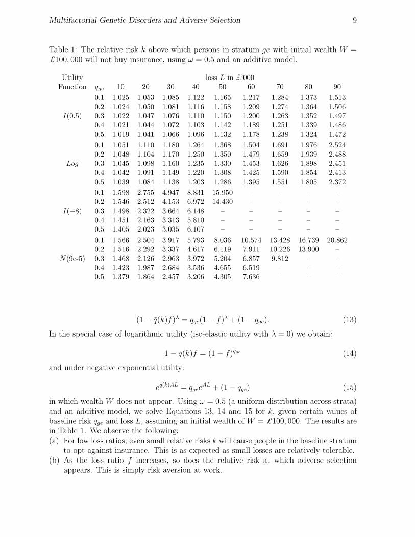
Multifactorial Genetic Disorders and Adverse Selection 9
Table 1: The relative risk k above which persons in stratum ge with initial wealth W =£100, 000 will not buy insurance, using ω = 0.5 and an additive model.
Utility loss L in £’000Function qge 10 20 30 40 50 60 70 80 90
0.1 1.025 1.053 1.085 1.122 1.165 1.217 1.284 1.373 1.5130.2 1.024 1.050 1.081 1.116 1.158 1.209 1.274 1.364 1.506
I(0.5) 0.3 1.022 1.047 1.076 1.110 1.150 1.200 1.263 1.352 1.4970.4 1.021 1.044 1.072 1.103 1.142 1.189 1.251 1.339 1.4860.5 1.019 1.041 1.066 1.096 1.132 1.178 1.238 1.324 1.472
0.1 1.051 1.110 1.180 1.264 1.368 1.504 1.691 1.976 2.5240.2 1.048 1.104 1.170 1.250 1.350 1.479 1.659 1.939 2.488
Log 0.3 1.045 1.098 1.160 1.235 1.330 1.453 1.626 1.898 2.4510.4 1.042 1.091 1.149 1.220 1.308 1.425 1.590 1.854 2.4130.5 1.039 1.084 1.138 1.203 1.286 1.395 1.551 1.805 2.372
0.1 1.598 2.755 4.947 8.831 15.950 – – – –0.2 1.546 2.512 4.153 6.972 14.430 – – – –
I(−8) 0.3 1.498 2.322 3.664 6.148 – – – – –0.4 1.451 2.163 3.313 5.810 – – – – –0.5 1.405 2.023 3.035 6.107 – – – – –
0.1 1.566 2.504 3.917 5.793 8.036 10.574 13.428 16.739 20.8620.2 1.516 2.292 3.337 4.617 6.119 7.911 10.226 13.900 –
N(9e-5) 0.3 1.468 2.126 2.963 3.972 5.204 6.857 9.812 – –0.4 1.423 1.987 2.684 3.536 4.655 6.519 – – –0.5 1.379 1.864 2.457 3.206 4.305 7.636 – – –
(1 − q(k)f)λ = qge(1 − f)λ + (1 − qge). (13)
In the special case of logarithmic utility (iso-elastic utility with λ = 0) we obtain:
1 − q(k)f = (1 − f)qge (14)
and under negative exponential utility:
eq(k)AL = qgeeAL + (1 − qge) (15)
in which wealth W does not appear. Using ω = 0.5 (a uniform distribution across strata)and an additive model, we solve Equations 13, 14 and 15 for k, given certain values ofbaseline risk qge and loss L, assuming an initial wealth of W = £100, 000. The results arein Table 1. We observe the following:(a) For low loss ratios, even small relative risks k will cause people in the baseline stratum
to opt against insurance. This is as expected as small losses are relatively tolerable.(b) As the loss ratio f increases, so does the relative risk at which adverse selection
appears. This is simply risk aversion at work.

Multifactorial Genetic Disorders and Adverse Selection 10
(c) The higher the baseline risk qge for a given loss ratio f , the lower the relative risk atwhich adverse selection appears.
(d) Lower risk-aversion, under iso-elastic utility, (λ = 0.5) means that smaller relativerisks would discourage members of the baseline stratum to buy insurance at theaverage premium, and for higher risk-aversion (λ = −8) the reverse is true.
Comparing iso-elastic and negative exponential utilities, we see that the limitingrelative risks are broadly similar for smaller losses. For larger losses, however, iso-elasticutility functions have much greater limiting relative risks. This is because risk-aversionincreases as wealth falls under iso-elastic utility, while for negative exponential utility itis constant. As the fair actuarial premium for bigger losses increases and depletes wealth,risk-aversion under iso-elastic utility climbs above that under negative exponential utility,with the result shown.
4.4 Immunity From Adverse Selection
The missing entries in Table 1 mean that adverse selection never appears, whateverthe relative risk k. Clearly, this must be related to the size of the high-risk strata, andtheir ability, or otherwise, to move the average premium enough to affect the baselinestratum. We may ask: given qge and f , is there some proportion wge in the lowest riskstratum above which members of that stratum will always buy insurance at the averagepremium rate? Begin by noting that:
limk→∞
q(k) = limk→∞
∑
s
ws[1 − (1 − qge)ks ] = wgeqge +
∑
s 6=ge
ws = 1 − wge(1 − qge) (16)
and that this limit is not a function of the ks and thus holds for additive and multiplicativemodels. Substituting this limiting value in Equations 13 to 15, we can solve for wge asfollows, for iso-elastic utility with λ 6= 0:
wge =1
1 − qge
[
1 −1 − (qge(1 − f)λ + (1 − qge))
1/λ
f
]
, (17)
for logarithmic utility:
wge =1
1 − qge
[
1 −1 − (1 − f)qge
f
]
(18)
and for negative exponential utility:
wge =1
1 − qge
[
1 −log[qgee
AL + (1 − qge)]
AL
]
. (19)
Values of ω = w1/2ge are given in Table 2. Values of ω < 0.5 in Table 2 correspond to
missing entries in Table 1. Table 2 shows just how uncommon an adverse exposure hasto be to avoid adverse selection.

Multifactorial Genetic Disorders and Adverse Selection 11
Table 2: The proportions ω exposed to each low-risk factor above which persons in thebaseline stratum will buy insurance at the average premium regardless of the relative riskk, using different utility functions.
Utility loss L in £’000Function qge 10 20 30 40 50 60 70 80 90
0.1 0.999 0.997 0.996 0.994 0.991 0.989 0.985 0.981 0.9740.2 0.997 0.994 0.991 0.987 0.983 0.977 0.970 0.961 0.947
I(0.5) 0.3 0.996 0.992 0.987 0.981 0.974 0.966 0.955 0.941 0.9190.4 0.995 0.989 0.982 0.974 0.965 0.954 0.940 0.920 0.8900.5 0.993 0.986 0.978 0.968 0.956 0.942 0.924 0.899 0.860
0.1 0.997 0.994 0.991 0.986 0.981 0.974 0.965 0.951 0.9260.2 0.995 0.989 0.981 0.973 0.962 0.949 0.932 0.906 0.859
Log 0.3 0.992 0.983 0.972 0.960 0.945 0.925 0.900 0.863 0.7980.4 0.989 0.977 0.963 0.947 0.927 0.902 0.870 0.823 0.7430.5 0.987 0.972 0.954 0.934 0.910 0.880 0.841 0.786 0.693
0.1 0.969 0.916 0.830 0.719 0.603 0.496 0.398 0.304 0.2030.2 0.943 0.857 0.747 0.632 0.525 0.431 0.345 0.264 0.176
I(−8) 0.3 0.919 0.812 0.693 0.580 0.480 0.393 0.315 0.241 0.1610.4 0.897 0.776 0.653 0.543 0.448 0.367 0.294 0.225 0.1500.5 0.878 0.746 0.622 0.515 0.424 0.347 0.279 0.213 0.142
0.1 0.971 0.927 0.868 0.802 0.738 0.682 0.635 0.595 0.5620.2 0.946 0.875 0.797 0.723 0.660 0.607 0.564 0.528 0.498
N(9e-5) 0.3 0.923 0.835 0.748 0.673 0.612 0.562 0.522 0.488 0.4610.4 0.903 0.802 0.712 0.637 0.577 0.530 0.492 0.460 0.4340.5 0.884 0.775 0.682 0.608 0.551 0.505 0.468 0.439 0.414

Multifactorial Genetic Disorders and Adverse Selection 12
Table 3: The relative risk k above which persons in stratum ge with initial wealth W =£100, 000 will not buy insurance, using ω = 0.9 and an additive model.
Utility loss L in £’000Function qge 10 20 30 40 50 60 70 80 90
0.1 1.126 1.269 1.433 1.625 1.855 2.140 2.511 3.033 3.8990.2 1.120 1.258 1.419 1.613 1.852 2.158 2.577 3.212 4.419
I(0.5) 0.3 1.113 1.246 1.404 1.599 1.847 2.180 2.668 3.502 5.6890.4 1.106 1.233 1.387 1.582 1.841 2.210 2.807 4.108 –0.5 1.099 1.218 1.367 1.562 1.833 2.250 3.055 – –
0.1 1.257 1.563 1.934 2.399 3.004 3.839 5.101 7.368 13.8410.2 1.246 1.546 1.923 2.418 3.107 4.170 6.164 13.981 –
Log 0.3 1.233 1.526 1.910 2.444 3.268 4.844 – – –0.4 1.220 1.504 1.894 2.482 3.555 8.317 – – –0.5 1.205 1.479 1.876 2.542 4.296 – – – –
0.1 4.458 18.642 – – – – – – –0.2 4.823 – – – – – – – –
I(−8) 0.3 5.705 – – – – – – – –0.4 – – – – – – – – –0.5 – – – – – – – – –
0.1 4.246 13.531 – – – – – – –0.2 4.514 – – – – – – – –
N(9e-5) 0.3 5.109 – – – – – – – –0.4 7.984 – – – – – – – –0.5 – – – – – – – – –
Assuming ω = 0.5 is perhaps extreme; it means that half the population possess asignificant genetic risk factor (modulated by environment) yet to be discovered. This isby no means impossible, but we might expect most as-yet unknown risk factors to affecta smaller proportion of the population, simply because they are as-yet unknown. So, weincrease ω to 0.9, so that only 10% of individuals are exposed to the adverse environmentor possess the adverse gene. The relative risks k at which adverse selection appears aregiven in Table 3. They are larger than in Table 1 because the relative risk experiencedby the smaller number of high-risk individuals has to be much higher to have the sameimpact on the average premium.
4.5 The Multiplicative Epidemiological Model
Table 4 shows relative risks above which adverse selection appears, assuming ω = 0.9and a multiplicative model. They can be compared with the values in Table 3. We observethe following:(a) The missing entries are the same as in the additive model. This is because the limiting
values of q(k) and ω do not depend on the model structure.(b) The relative risk in stratum GE is higher in the multiplicative model (k2 > 2k − 1)
so persons in the baseline stratum will be less tolerant towards any given value of k.
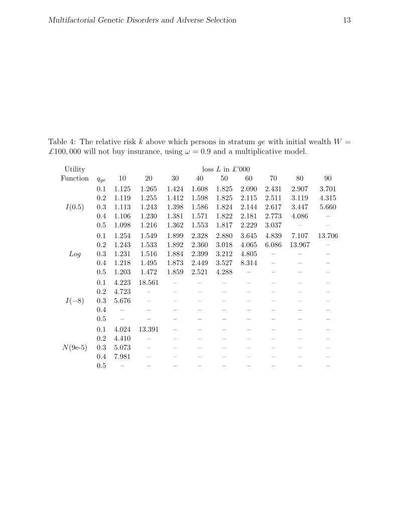
Multifactorial Genetic Disorders and Adverse Selection 13
Table 4: The relative risk k above which persons in stratum ge with initial wealth W =£100, 000 will not buy insurance, using ω = 0.9 and a multiplicative model.
Utility loss L in £’000Function qge 10 20 30 40 50 60 70 80 90
0.1 1.125 1.265 1.424 1.608 1.825 2.090 2.431 2.907 3.7010.2 1.119 1.255 1.412 1.598 1.825 2.115 2.511 3.119 4.315
I(0.5) 0.3 1.113 1.243 1.398 1.586 1.824 2.144 2.617 3.447 5.6600.4 1.106 1.230 1.381 1.571 1.822 2.181 2.773 4.086 –0.5 1.098 1.216 1.362 1.553 1.817 2.229 3.037 – –
0.1 1.254 1.549 1.899 2.328 2.880 3.645 4.839 7.107 13.7060.2 1.243 1.533 1.892 2.360 3.018 4.065 6.086 13.967 –
Log 0.3 1.231 1.516 1.884 2.399 3.212 4.805 – – –0.4 1.218 1.495 1.873 2.449 3.527 8.314 – – –0.5 1.203 1.472 1.859 2.521 4.288 – – – –
0.1 4.223 18.561 – – – – – – –0.2 4.723 – – – – – – – –
I(−8) 0.3 5.676 – – – – – – – –0.4 – – – – – – – – –0.5 – – – – – – – – –
0.1 4.024 13.391 – – – – – – –0.2 4.410 – – – – – – – –
N(9e-5) 0.3 5.073 – – – – – – – –0.4 7.981 – – – – – – – –0.5 – – – – – – – – –

Multifactorial Genetic Disorders and Adverse Selection 14
This is why the values in Table 4 are smaller than those in Table 3.(c) However the differences between the additive and multiplicative models are not very
large. If k ≈ 1, then k2 ≈ 2k − 1, and for large values of ω (which arguably is mostrealistic) the impact of stratum GE is relatively small. In view of this, we will useonly the additive model from now on.
4.6 Loss versus Coverage
Our simple model assumes that everyone risks the same loss L, and chooses to insureit 100% if they insure at all. A more realistic model, as pointed out by a referee, mightassume that persons knowing themselves to be in stratum s choose insurance cover ofCs, not necessarily equal to L (indeed not necessarily bounded by L unless the insurerlimits the coverage by reference to some objective measure of L or W ). Assuming theinsurer charges an average premium rate q(k) as before, Cs will be chosen to maximiseqsU(W −L+Cs− q(k)Cs)+(1−qs)U(W − q(k)Cs). This extension of the model would beof interest in its own right; however some experiments (not shown) confirm that it doesnot change the qualitative nature of our conclusions.
4.7 Genetic Information and Behaviour
The introduction of new genetic information — ability to learn one’s own genotype— may lead high-risk people in particular to alter their behaviour to ameliorate therisk. Thus the composition of the risk groups may not be the same before and aftergenetic testing (say) becomes available. This possibility is more plausible for multifactorialdiseases than for single-gene disorders, since there will often be modifiable environmentalor lifestyle interactions. For example, if our environmental variable was E = ‘smoker’ ande = ‘non-smoker’, persons initially in stratum GE might be particularly likely to stopsmoking, and (perhaps after some time) move to stratum Ge. The low-risk strata willbe enlarged, which will: (a) cause the weighted average premium to fall; and (b) as inTable 2, make it more likely that low-risk individuals will buy insurance regardless of therelative risks. Therefore, our results err on the pessimistic side.
Such behavioural effects can, in principle, be modelled by allowing transitions betweenstrata, after genetic testing and before insurance is purchased. For example, supposeω = 0.9 and 1% of the population is initially in stratum GE, but that after genetic testsbecome available, half of those in stratum GE move to stratum Ge. Table 3 shows therelative risk thresholds before, and Table 5 after, the introduction of genetic tests. Thereis an appreciable difference, even though only 0.5% of the population has changed itsbehaviour. However, since we have no greater insight than this into how behaviour mightchange, we interpret all our results except those in Table 5 as being after any behaviouralchanges have taken effect. When real epidemiological studies eventually become available,the effect of modified behaviour should not be overlooked.
5. Critical Illness Insurance
5.1 A Heart Attack Model
We now model the specific example of CI insurance. We will focus on heart attackrisk, building upon two earlier papers, in which the reader can find full details.

Multifactorial Genetic Disorders and Adverse Selection 15
Table 5: The relative risk k above which persons in stratum ge with initial wealth W =£100, 000 will not buy insurance, using wge = 0.81, wGe = 0.095, wgE = 0.09 and wGE =0.005 and an additive model.
Utility loss L in £’000Function qge 10 20 30 40 50 60 70 80 90
0.1 1.167 1.356 1.571 1.821 2.118 2.482 2.949 3.597 4.6490.2 1.159 1.339 1.548 1.794 2.092 2.468 2.971 3.714 5.078
I(0.5) 0.3 1.150 1.321 1.523 1.765 2.067 2.462 3.023 3.951 6.2720.4 1.140 1.302 1.496 1.734 2.040 2.463 3.125 4.508 –0.5 1.129 1.282 1.466 1.699 2.012 2.478 3.339 – –
0.1 1.341 1.741 2.219 2.808 3.561 4.576 6.071 8.662 15.6740.2 1.324 1.709 2.180 2.781 3.593 4.801 6.974 15.032 –
Log 0.3 1.306 1.675 2.142 2.767 3.693 5.389 – – –0.4 1.286 1.640 2.102 2.768 3.928 8.788 – – –0.5 1.265 1.601 2.061 2.794 4.621 – – – –
0.1 5.315 20.677 – – – – – – –0.2 5.523 – – – – – – – –
I(−8) 0.3 6.288 – – – – – – – –0.4 – – – – – – – – –0.5 – – – – – – – – –
0.1 5.063 15.347 – – – – – – –0.2 5.182 – – – – – – – –
N(9e-5) 0.3 5.666 – – – – – – – –0.4 8.454 – – – – – – – –0.5 – – – – – – – – –

Multifactorial Genetic Disorders and Adverse Selection 16
(a) Gutierrez & Macdonald (2003) parameterised the CI model shown in Figure 2, usingmedical studies and population data. Therefore, in particular, λ12(x) denotes the rateof onset of heart attacks in the general population (different for males and females).
(b) Macdonald, Pritchard & Tapadar (2006) assumed that a 2 × 2 gene-environmentinteraction affected heart attack risk, with genotypes G and g, and environmentalexposures E and e, upper case representing higher risk. So there are four strata foreach sex — ge, gE,Ge and GE. The authors showed that it is possible to hypothecateassumptions on strata-specific relative risks, in a way which is consistent with the rateof onset in the general population. We will use a similar technique here.
������������*
��
��
��
��
��
���
-@
@@
@@
@@
@@
@@@R
HHHHHHHHHHHHj
State 6 Dead
State 5 Other CI
State 4 Stroke
State 3 Cancer
State 2 Heart Attack
State 1 Healthy
λ12(x)
λ13(x)
λ14(x)
λ15(x)
λ16(x)
Figure 2: A full critical illness model.
Consider all healthy individuals aged x. If q denotes the probability that a healthyperson aged x has a heart attack before age x + t, it can be calculated from the heartattack transition intensity of the general population as follows:
q = 1 − exp
[
−
∫ t
0
λ12(x + y)dy
]
(20)
Now, for males and females separately, let c denote the relative risk in the baselinestratum ge with respect to the general population, and let ks denote the relative risk instratum s with respect to stratum ge, in both cases assumed to be constant at all ages
Multifactorial Genetic Disorders and Adverse Selection 17
0
0.2
0.4
0.6
0.8
1
0 10 20 30 40 50 60 70 80
Rat
io
Age (years)
MaleFemale
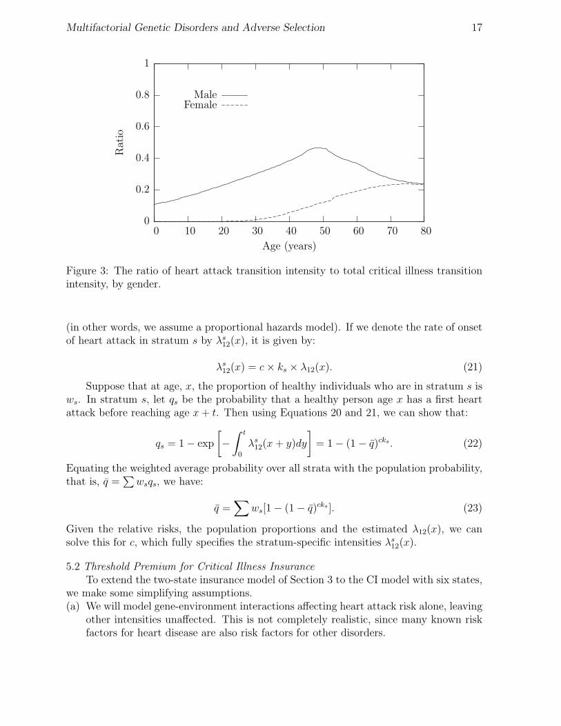
Figure 3: The ratio of heart attack transition intensity to total critical illness transitionintensity, by gender.
(in other words, we assume a proportional hazards model). If we denote the rate of onsetof heart attack in stratum s by λs
12(x), it is given by:
λs12(x) = c × ks × λ12(x). (21)
Suppose that at age, x, the proportion of healthy individuals who are in stratum s isws. In stratum s, let qs be the probability that a healthy person age x has a first heartattack before reaching age x + t. Then using Equations 20 and 21, we can show that:
qs = 1 − exp
[
−
∫ t
0
λs12(x + y)dy
]
= 1 − (1 − q)cks . (22)
Equating the weighted average probability over all strata with the population probability,that is, q =
∑
wsqs, we have:
q =∑
ws[1 − (1 − q)cks ]. (23)
Given the relative risks, the population proportions and the estimated λ12(x), we cansolve this for c, which fully specifies the stratum-specific intensities λs
12(x).
5.2 Threshold Premium for Critical Illness Insurance
To extend the two-state insurance model of Section 3 to the CI model with six states,we make some simplifying assumptions.(a) We will model gene-environment interactions affecting heart attack risk alone, leaving
other intensities unaffected. This is not completely realistic, since many known riskfactors for heart disease are also risk factors for other disorders.
Multifactorial Genetic Disorders and Adverse Selection 18
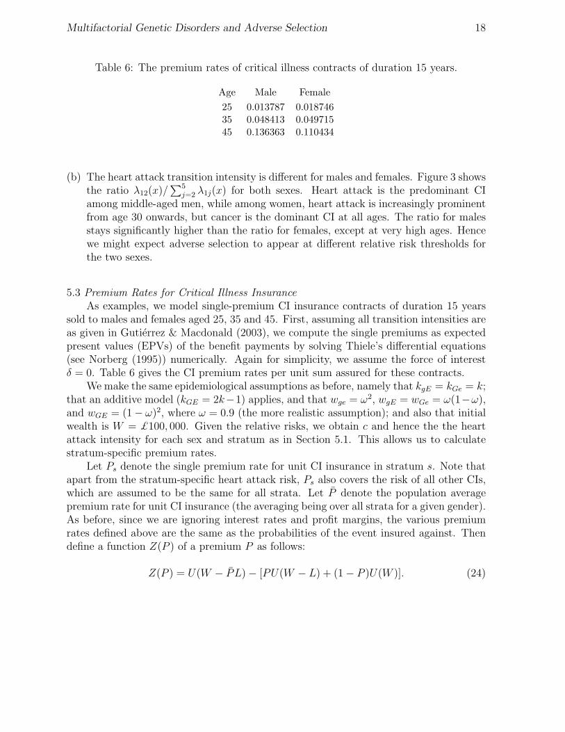
Table 6: The premium rates of critical illness contracts of duration 15 years.
Age Male Female
25 0.013787 0.01874635 0.048413 0.04971545 0.136363 0.110434
(b) The heart attack transition intensity is different for males and females. Figure 3 showsthe ratio λ12(x)/
∑5j=2 λ1j(x) for both sexes. Heart attack is the predominant CI
among middle-aged men, while among women, heart attack is increasingly prominentfrom age 30 onwards, but cancer is the dominant CI at all ages. The ratio for malesstays significantly higher than the ratio for females, except at very high ages. Hencewe might expect adverse selection to appear at different relative risk thresholds forthe two sexes.
5.3 Premium Rates for Critical Illness Insurance
As examples, we model single-premium CI insurance contracts of duration 15 yearssold to males and females aged 25, 35 and 45. First, assuming all transition intensities areas given in Gutierrez & Macdonald (2003), we compute the single premiums as expectedpresent values (EPVs) of the benefit payments by solving Thiele’s differential equations(see Norberg (1995)) numerically. Again for simplicity, we assume the force of interestδ = 0. Table 6 gives the CI premium rates per unit sum assured for these contracts.
We make the same epidemiological assumptions as before, namely that kgE = kGe = k;that an additive model (kGE = 2k−1) applies, and that wge = ω2, wgE = wGe = ω(1−ω),and wGE = (1 − ω)2, where ω = 0.9 (the more realistic assumption); and also that initialwealth is W = £100, 000. Given the relative risks, we obtain c and hence the the heartattack intensity for each sex and stratum as in Section 5.1. This allows us to calculatestratum-specific premium rates.
Let Ps denote the single premium rate for unit CI insurance in stratum s. Note thatapart from the stratum-specific heart attack risk, Ps also covers the risk of all other CIs,which are assumed to be the same for all strata. Let P denote the population averagepremium rate for unit CI insurance (the averaging being over all strata for a given gender).As before, since we are ignoring interest rates and profit margins, the various premiumrates defined above are the same as the probabilities of the event insured against. Thendefine a function Z(P ) of a premium P as follows:
Z(P ) = U(W − PL) − [PU(W − L) + (1 − P )U(W )]. (24)
Mult
ifactoria
lG
enetic
Dis
orders
and
Adverse
Sele
ctio
n19
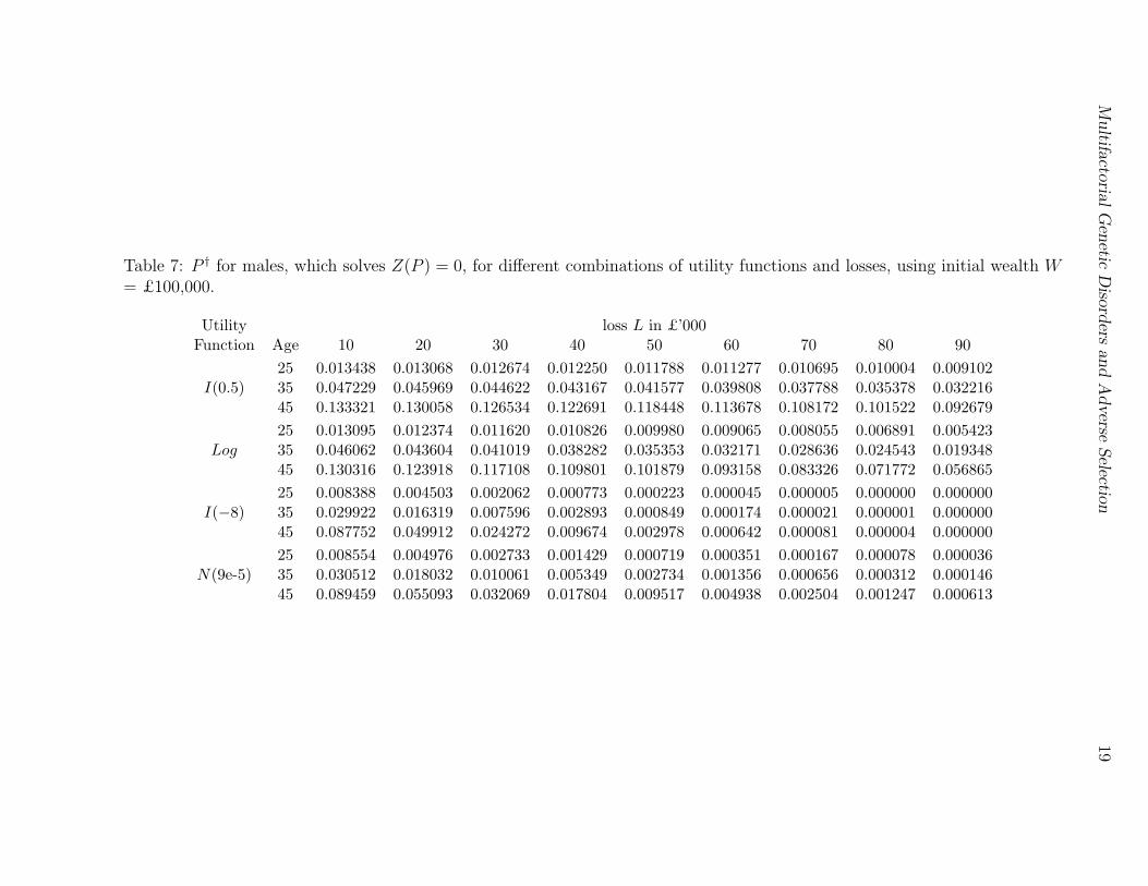
Table 7: P † for males, which solves Z(P ) = 0, for different combinations of utility functions and losses, using initial wealth W= £100,000.
Utility loss L in £’000Function Age 10 20 30 40 50 60 70 80 90
25 0.013438 0.013068 0.012674 0.012250 0.011788 0.011277 0.010695 0.010004 0.009102I(0.5) 35 0.047229 0.045969 0.044622 0.043167 0.041577 0.039808 0.037788 0.035378 0.032216
45 0.133321 0.130058 0.126534 0.122691 0.118448 0.113678 0.108172 0.101522 0.092679
25 0.013095 0.012374 0.011620 0.010826 0.009980 0.009065 0.008055 0.006891 0.005423Log 35 0.046062 0.043604 0.041019 0.038282 0.035353 0.032171 0.028636 0.024543 0.019348
45 0.130316 0.123918 0.117108 0.109801 0.101879 0.093158 0.083326 0.071772 0.056865
25 0.008388 0.004503 0.002062 0.000773 0.000223 0.000045 0.000005 0.000000 0.000000I(−8) 35 0.029922 0.016319 0.007596 0.002893 0.000849 0.000174 0.000021 0.000001 0.000000
45 0.087752 0.049912 0.024272 0.009674 0.002978 0.000642 0.000081 0.000004 0.000000
25 0.008554 0.004976 0.002733 0.001429 0.000719 0.000351 0.000167 0.000078 0.000036N(9e-5) 35 0.030512 0.018032 0.010061 0.005349 0.002734 0.001356 0.000656 0.000312 0.000146
45 0.089459 0.055093 0.032069 0.017804 0.009517 0.004938 0.002504 0.001247 0.000613

Mult
ifactoria
lG
enetic
Dis
orders
and
Adverse
Sele
ctio
n20
Table 8: P † for females, which solves Z(P ) = 0, for different combinations of utility functions and losses, using initial wealthW = £100,000.
Utility loss L in £’000Function Age 10 20 30 40 50 60 70 80 90
25 0.018273 0.017773 0.017239 0.016664 0.016038 0.015344 0.014554 0.013616 0.012389I(0.5) 35 0.048500 0.047209 0.045827 0.044334 0.042702 0.040886 0.038813 0.036339 0.033093
45 0.107899 0.105188 0.102269 0.099094 0.095600 0.091684 0.087179 0.081758 0.074580
25 0.017809 0.016833 0.015811 0.014734 0.013586 0.012344 0.010971 0.009388 0.007390Log 35 0.047304 0.044782 0.042131 0.039322 0.036315 0.033050 0.029420 0.025217 0.019880
45 0.105398 0.100089 0.094460 0.088443 0.081945 0.074821 0.066825 0.057471 0.045463
25 0.011431 0.006150 0.002823 0.001060 0.000307 0.000062 0.000007 0.000000 0.000000I(−8) 35 0.030745 0.016778 0.007814 0.002978 0.000875 0.000180 0.000021 0.000001 0.000000
45 0.070219 0.039438 0.018924 0.007438 0.002256 0.000479 0.000059 0.000003 0.000000
25 0.011657 0.006796 0.003740 0.001961 0.000989 0.000483 0.000231 0.000108 0.000050N(9e-5) 35 0.031351 0.018539 0.010350 0.005506 0.002817 0.001397 0.000677 0.000322 0.000151
45 0.071593 0.043550 0.025029 0.013714 0.007231 0.003700 0.001849 0.000908 0.000439

Multifactorial Genetic Disorders and Adverse Selection 21
Table 9: The population average premium rate for CI insurance, P0, as if heart attackrisk were absent (λ12 = 0).
Age Male Female
25 0.009821 0.01832635 0.031290 0.04648545 0.092818 0.097947
Note that Z(Pge) < 0 is the condition under which adverse selection will appear, equivalentto Equation 12 of Section 4.2. Or, let P † be the solution of Z(P ) = 0. Then Pge < P †
is the condition for adverse selection to appear. Tables 7 and 8 show P † for males andfemales respectively. It depends on the utility function but not on the epidemiologicalmodel. For the 2-state model, Equation 12 was central in our analysis. Given: (a) amodel structure (additive or multiplicative), the baseline risk qge, and the proportion ωwith low values of each risk factor; and (b) noting that the average risk q was an increasingfunction of the relative risk parameter k; we obtained a minimum value of k for whichadverse selection first appears.
We would like to do the same for the CI insurance model. However, there are impor-tant differences between the two models.(a) In the 2-state model we specified the baseline risk and relative risks, and these deter-
mined the average risk. In the CI insurance model, we specify the average risk (givenby the population heart attack risk) and the relative risks, and these determine thebaseline risk, in the form of the relative risk c. Clearly increasing the relative riskk will cause c to fall, hence also the premium Pge. To make this dependence clear,we will write c(k) and Pge(k) in this section. It will also be useful to note that theprobability qge of a heart attack similarly depends on k, and write qge(k).
(b) However, unlike in the 2-state model, Pge(k) has a lower bound, denoted P0, givenby the population average premium rate for CI insurance as if heart attack risk wereabsent (λ12 = 0 and c = 0). These values are shown in Table 9. They do not depend onthe epidemiological model or the utility function. Clearly Pge(k) ≥ P0, no matter howhigh k becomes. Thus we have two possibilities: limk→∞ Pge(k) = P0 (equivalentlylimk→∞ c(k) = 0); or limk→∞ Pge(k) > P0 (equivalently limk→∞ c(k) > 0). We returnto this point in Section 5.4.
(c) If Pge(k) is a strictly decreasing function, which it is for the utility functions weare using, adverse selection is possible if limk→∞ Pge(k) < P †, and in such cases wecan solve Pge(k) = P † for the threshold value of k above which adverse selectionwill appear. Tables 10 and 11 show these values for the various utility functionsand loss levels, for males and females respectively. The missing values correspond tocombinations of parameters such that limk→∞ Pge(k) > P †, for which adverse selectionwill not appear.
(d) Another consequence of this is that there is a level of insured loss, that we denote L0,above which adverse selection cannot occur, because fixing L > L0 in Equation 24and solving for P † yields a solution P † < Pge(k) for all k. Table 12 gives the valuesof L0, for the usual utility functions and initial wealth £100,000. The missing values

Multifactorial Genetic Disorders and Adverse Selection 22
Table 10: The relative risk k above which males of different ages in stratum ge withinitial wealth W = £100, 000 will not buy critical illness insurance policies of term 15years, where ω = 0.9.
Utility loss L in £’000Function Age 10 20 30 40 50 60 70 80 90
25 1.484 2.111 2.960 4.183 6.117 9.698 18.869 105.569 –I(0.5) 35 1.376 1.846 2.450 3.262 4.420 6.226 9.509 17.715 93.578
45 1.389 1.886 2.544 3.456 4.808 7.027 11.388 24.239 –
25 2.062 3.783 7.068 15.883 122.410 – – – –Log 35 1.808 2.998 4.917 8.530 17.855 98.596 – – –
45 1.843 3.138 5.339 9.794 23.063 765.192 – – –
25 – – – – – – – – –I(−8) 35 – – – – – – – – –
45 – – – – – – – – –
25 – – – – – – – – –N(9e-5) 35 – – – – – – – – –
45 – – – – – – – – –
Table 11: The relative risk k above which females of different ages in stratum ge withinitial wealth W = £100, 000 will not buy critical illness insurance policies of term 15years, where ω = 0.9.
Utility loss L in £’000Function Age 10 20 30 40 50 60 70 80 90
25 – – – – – – – – –I(0.5) 35 4.031 18.470 – – – – – – –
45 2.293 4.710 10.770 52.668 – – – – –
25 – – – – – – – – –Log 35 15.856 – – – – – – – –
45 4.459 26.155 – – – – – – –
25 – – – – – – – – –I(−8.0) 35 – – – – – – – – –
45 – – – – – – – – –
25 – – – – – – – – –N(9e-5) 35 – – – – – – – – –
45 – – – – – – – – –

Multifactorial Genetic Disorders and Adverse Selection 23
Table 12: The loss L0 in £,000 above which adverse selection cannot occur. Initial wealthW = £100,000.
Utility FunctionGender Age I(0.5) Log I(−8) N(9e-5)
25 82.3 51.8 7.1 7.2Male 35 92.3 62.6 9.2 9.5
45 89.9 60.4 8.9 9.2
25 8.9 4.5 0.5 0.5Female 35 25.3 13.3 1.5 1.6
45 43.4 23.9 2.9 2.9
in Tables 10 and 11 occur for losses L > L0.
The general pattern of threshold relative risks for males given in Table 10 is similarto that in Section 4; what is of most interest are their absolute values, since we have triedto suggest plausible models for both the risk model and the utility functions.(a) For iso-elastic utility with λ = −8 and negative exponential utility with parameter
A = 9 × 10⁻⁵, we find no evidence at all of adverse selection.(b) For all utility functions and at all loss levels, if adverse selection can appear, it does
so at higher levels of relative risk than under the two-state model. This is because theimpact of the gene and environment on heart attack risk is diluted by the presenceof the other CIs, whose risks are assumed to be independent of the g/G genotypesand e/E environments. Only for the lowest levels of loss are these relative risks inthe range that might be typical of relatively common multifactorial disorders; bydefinition, we do not expect studies like UK Biobank to lead to the discovery ofhitherto unknown high risk genotypes.
(c) When adverse selection can appear, the relative risk threshold first decreases and thenincreases with age. This is because among CIs the importance of heart attack peaksat around age 45 as can be seen from Figure 6.
The threshold relative risks for females are given in Table 11. We observe the follow-ing:(a) The threshold relative risks are much higher than those for males, in all cases. This
is because heart attacks form a smaller proportion of all CIs for females, so a largerincrease in heart attack risk is needed to trigger adverse selection.
(b) As for males, at levels of absolute and relative risk-aversion that we regard as mostplausible (consistent with the Bank of Italy study) we find no evidence that adverseselection is likely.
(c) In contrast to males, the threshold relative risks decrease with age. The reason isclear from Figure 3; for females the relative importance of heart attack increases withage.
(d) Adverse selection appears to be possible only for: (i) smaller losses; and (ii) extremelylow levels of risk aversion.

Multifactorial Genetic Disorders and Adverse Selection 24
5.4 High Relative Risks
In Section 4.4, we considered relative risks that increased without limit, for the simple2-state insurance model. We saw that, even in this extreme case, if stratum ge was largeenough, adverse selection would not appear. In this section, we consider high relativerisks (of heart attack) in the CI insurance model.
We assume the heart attack rates in the general population λ12(x) are fixed at theirestimated values (Gutierrez & Macdonald, 2003). From Equation 23 we obtain:
1 − q = 1 −∑
s
ws[1 − (1 − q)c(k)ks ]
= wge(1 − q)c +∑
s 6=ge
ws(1 − q)cks . (25)
Differentiation shows the right-hand side to be a decreasing function of c and of each ks
(s 6= ge), all other quantities held constant in each case. Also, if c = 1 the right-hand sideis less than (1 − q) while if c = 0 it is greater than (1 − q). Hence, as we increase the ks
without limit, c must decrease, and being bounded below it must have a limit. The limitcould be zero or non-zero. We can easily see that if c has a non-zero limit (necessarilypositive) then the last term on the right-hand side of Equation 25 vanishes and the limitmust be:
limks→∞s 6=ge
c = 1 −log wge
log(1 − q)(26)
which in turn implies (1 − q) < wge. On the other hand if (1 − q) > wge, then c cannothave non-zero limit, so the equation:
limks→∞s 6=ge
∑
s 6=ge
ws(1 − q)cks = (1 − q) − wge (27)
holds. Since the left-hand side is finite, at least one of the products cks tends to a finitelimit as the ks → ∞. However, we have not specified here how the quantities ks (s 6= ge)jointly approach infinity, so the behaviour of c is not easy to analyse in general. It isgreatly simplified if the ks are simple functions of a single parameter k, which is thecase in our assumed epidemiological model (in which case we again make explicit thedependence of c by writing c(k)). For example, under an additive model with symmetrybetween genetic and environmental risks, Equation 25 can be written as:
1 − q = ω2(1 − q)c + 2ω(1 − ω)(1 − q)c(k)k + (1 − ω)2(1 − q)c(k)(2k−1)
= (1 − q)c(k)[ω + (1 − ω)(1 − q)c(k)(k−1)]2 (28)
therefore:
k = 1 +log[(1 − q)(1−c(k))/2 − ω] − log(1 − ω)
c(k) log(1 − q). (29)
Multifactorial Genetic Disorders and Adverse Selection 25
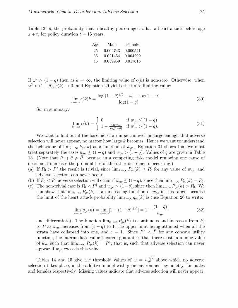
Table 13: q, the probability that a healthy person aged x has a heart attack before agex + t, for policy duration t = 15 years.
Age Male Female
25 0.004743 0.00054135 0.021454 0.00429945 0.059959 0.017616
If ω2 > (1 − q) then as k → ∞, the limiting value of c(k) is non-zero. Otherwise, whenω2 < (1 − q), c(k) → 0, and Equation 29 yields the finite limiting value:
limk→∞
c(k)k =log[(1 − q)1/2 − ω] − log(1 − ω)
log(1 − q). (30)
So, in summary:
limk→∞
c(k) =
{
0 if wge ≤ (1 − q)
1 −log wge
log(1−q)if wge > (1 − q).
(31)
We want to find out if the baseline stratum ge can ever be large enough that adverseselection will never appear, no matter how large k becomes. Hence we want to understandthe behaviour of limk→∞ Pge(k) as a function of wge. Equation 31 shows that we musttreat separately the cases wge ≤ (1− q) and wge > (1− q). Values of q are given in Table13. (Note that P0 + q 6= P , because in a competing risks model removing one cause ofdecrement increases the probabilities of the other decrements occurring.)(a) If P0 > P † the result is trivial, since limk→∞ Pge(k) ≥ P0 for any value of wge, and
adverse selection can never occur.(b) If P0 < P † adverse selection will occur if wge ≤ (1−q), since then limk→∞ Pge(k) = P0.(c) The non-trivial case is P0 < P † and wge > (1− q), since then limk→∞ Pge(k) > P0. We
can show that limk→∞ Pge(k) is an increasing function of wge in this range, becausethe limit of the heart attack probability limk→∞ qge(k) is (use Equation 26 to write:
limk→∞
qge(k) = limk→∞
[1 − (1 − q)c(k)] = 1 −(1 − q)
wge
(32)
and differentiate). The function limk→∞ Pge(k) is continuous and increases from P0
to P as wge increases from (1 − q) to 1, the upper limit being attained when all thestrata have collapsed into one, and c = 1. Since P † < P for any concave utilityfunction, the intermediate value theorem guarantees that there exists a unique valueof wge such that limk→∞ Pge(k) = P †; that is, such that adverse selection can neverappear if wge exceeds this value.
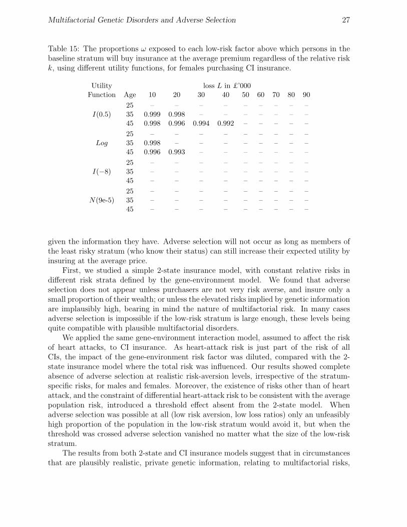
Tables 14 and 15 give the threshold values of ω = w1/2ge above which no adverse
selection takes place, in the additive model with gene-environment symmetry, for malesand females respectively. Missing values indicate that adverse selection will never appear.

Multifactorial Genetic Disorders and Adverse Selection 26
Table 14: The proportions ω exposed to each low-risk factor above which persons in thebaseline stratum will buy insurance at the average premium regardless of the relative riskk, using different utility functions, for males purchasing CI insurance.
Utility loss L in £’000Function Age 10 20 30 40 50 60 70 80 90
25 1.000 1.000 0.999 0.999 0.999 0.998 0.998 0.998 –I(0.5) 35 0.999 0.998 0.998 0.997 0.996 0.995 0.993 0.992 0.990
45 0.998 0.995 0.993 0.990 0.987 0.984 0.980 0.975 –
25 1.000 0.999 0.999 0.998 0.998 – – – –Log 35 0.999 0.997 0.995 0.994 0.992 0.990 – – –
45 0.996 0.991 0.986 0.981 0.976 0.970 – – –
25 – – – – – – – – –I(−8) 35 – – – – – – – – –
45 – – – – – – – – –
25 – – – – – – – – –N(9e-5) 35 – – – – – – – – –
45 – – – – – – – – –
When it is possible, the threshold value of ω ranges from 0.970 to 1 for males and 0.992to 0.999 for females. As the relative risks in Tables 10 and 11 are based on ω = 0.9, thisexplains the missing values in those tables.
This pattern is quite unexpected. If adverse selection can occur, then a large enoughbaseline stratum does confer immunity from it, but it has to be very large indeed, allbut a few percent of the population. But once the threshold is crossed, adverse selectioncannot appear at all, even if very few people are in the baseline stratum. This had nocounterpart in the 2-state model, and it is caused by the presence of substantial otherrisks not affected by the gene-environment variants.
6. Conclusions
Until now, genetical research on information asymmetry and adverse selection hastaken one of two routes — models of single-gene disorders and work on the economicwelfare effects of genetic testing. In this paper, we have represented multifactorial disor-ders using standard epidemiological models and analysed circumstances leading to adverseselection, taking economic factors into account in a simple way through expected utility.
We used a range of iso-elastic utilities (including the special case of logarithmic utility)and a negative exponential utility, to represent constant relative and absolute risk aversion,respectively. They were parameterised to be reasonably consistent with some estimatesbased on survey data, but also to allow comparability, given our chosen level of wealth of£100,000.
We used a simple 2 × 2 gene-environment interaction model, assuming that informa-tion on status within the model was available only to the consumers and not to the insurer.Competition leads insurers to charge actuarially fair premiums, based on expected losses
Multifactorial Genetic Disorders and Adverse Selection 27
Table 15: The proportions ω exposed to each low-risk factor above which persons in thebaseline stratum will buy insurance at the average premium regardless of the relative riskk, using different utility functions, for females purchasing CI insurance.
Utility loss L in £’000Function Age 10 20 30 40 50 60 70 80 90
25 – – – – – – – – –I(0.5) 35 0.999 0.998 – – – – – – –
45 0.998 0.996 0.994 0.992 – – – – –
25 – – – – – – – – –Log 35 0.998 – – – – – – – –
45 0.996 0.993 – – – – – – –
25 – – – – – – – – –I(−8) 35 – – – – – – – – –
45 – – – – – – – – –
25 – – – – – – – – –N(9e-5) 35 – – – – – – – – –
45 – – – – – – – – –
given the information they have. Adverse selection will not occur as long as members ofthe least risky stratum (who know their status) can still increase their expected utility byinsuring at the average price.
First, we studied a simple 2-state insurance model, with constant relative risks indifferent risk strata defined by the gene-environment model. We found that adverseselection does not appear unless purchasers are not very risk averse, and insure only asmall proportion of their wealth; or unless the elevated risks implied by genetic informationare implausibly high, bearing in mind the nature of multifactorial risk. In many casesadverse selection is impossible if the low-risk stratum is large enough, these levels beingquite compatible with plausible multifactorial disorders.
We applied the same gene-environment interaction model, assumed to affect the riskof heart attacks, to CI insurance. As heart-attack risk is just part of the risk of allCIs, the impact of the gene-environment risk factor was diluted, compared with the 2-state insurance model where the total risk was influenced. Our results showed completeabsence of adverse selection at realistic risk-aversion levels, irrespective of the stratum-specific risks, for males and females. Moreover, the existence of risks other than of heartattack, and the constraint of differential heart-attack risk to be consistent with the averagepopulation risk, introduced a threshold effect absent from the 2-state model. Whenadverse selection was possible at all (low risk aversion, low loss ratios) only an unfeasiblyhigh proportion of the population in the low-risk stratum would avoid it, but when thethreshold was crossed adverse selection vanished no matter what the size of the low-riskstratum.
The results from both 2-state and CI insurance models suggest that in circumstancesthat are plausibly realistic, private genetic information, relating to multifactorial risks,

Multifactorial Genetic Disorders and Adverse Selection 28
that is available only to customers does not lead to adverse selection. This conclusion isstrongest in the more realistic CI insurance model.
We have not considered what might happen if insurers were allowed access to thisgenetic information. The opportunity would then exist to underwrite using that informa-tion. If one believed that social policy is best served by solidarity, the important questionis whether insurers would find it worthwhile to use the genetic information. Furtherresearch would be useful, to investigate the costs of acquiring and interpreting geneticinformation relating to common diseases, compared with the benefits in terms of possiblymore accurate risk classification, in both cases in the context of multifactorial risk.
Acknowledgements
This work was carried out at the Genetics and Insurance Research Centre at Heriot-Watt University. We would like to thank the sponsors for funding, and members of theSteering Committee for helpful comments at various stages. We would also like to thankan anonymous referee for very constructive comments.
References
Abel, A. (1986). Capital accumulation and uncertain lifetimes with adverse selection. Econo-metrica, 54, 1079–97.
Binmore, K. (1991). Fun and games: A text on game theory. Houghton Mifflin.
Brugiavini, A. (1993). Uncertainty resolution and the timing of annuity purchases. Journalof Public Economics, 50, 31–62.
Doherty, N.A. & Thistle, P.D. (1996). Adverse selection with endogeneous information ininsurance markets. Journal of Public Economics, 63, 83–102.
Eisenhauer, J.G. & Ventura, L. (2003). Survey measures of risk aversion and prudence.Applied Economics, 35, 1477–1484.
Guiso, L. & Paiella, M. (2006), The role of risk aversion in predicting individual behavior, inCompetitive Failures in Insurance Markets: Theory and Policy Implications, eds. Chiappori,P.-A. & Gollier, C., MIT Press.
Gutierrez, C. & Macdonald, A.S. (2003). Adult polycystic kidney disease and criticalillness insurance. North American Actuarial Journal, 7:2, 93–115.
H.M. Treasury (2005). Economy charts and tables. Pre-Budget Report.
Hoy, M. (2006). Risk classification and social welfare. The Geneva Papers of Risk and Insur-ance: Issues and Practice, 31, 245–269.
Hoy, M. & Polborn, M. (2000). The value of genetic information in the life insurance market.Journal of Public Economics, 78, 235–252.
Hoy, M. & Witt, J. (2007). Welfare effects of banning genetic information in the life insurancemarket: The case of BRCA1/2 genes. Journal of Risk and Insurance, 74:3, 523–546.
Jones, F. (2005). The effects of taxes and benefits on household income, 2004/05. Office forNational Statistics.
Macdonald, A.S. (2004), Genetics and Insurance, in Encyclopaedia of Actuarial Science, ed.Teugels, J. & Sundt, B., John Wiley, Chichister.

Multifactorial Genetic Disorders and Adverse Selection 29
Macdonald, A.S., Pritchard, D.J. & Tapadar, P. (2006). The impact of multifactorialgenetic disorders on critical illness insurance: A simulation study based on UK Biobank.ASTIN Bulletin, 36, 311–346.
Meyer, D.J. & Meyer, J. (2005). Risk preferences in multi-period consumption models, theequity premium puzzle and habit formation utility. Journal of Monetary Economics, 52,1497–1515.
Norberg, R. (1995). Differential equations for moments of present values in life insurance.Insurance: Mathematics and Economics, 17, 171–180.
Polborn, M., Hoy, M. & Sadanand, A. (2006). Advantageous effects of regulatory adverseselection in the life insurance market. Economic Journal, 116, 327–354.
Subramanian, K., Lemaire, J., Hershey, J.C., Pauly, M.V., Armstrong, K. & Asch,
D.A. (1999). Estimating adverse selection costs from genetic testing for breast and ovariancancer: The case of life insurance. Journal of Risk and Insurance, 66:4, 531–550.
Villeneuve, B. (1999). Mandatory insurance and the intensity of adverse selection. CREST/INSEEworking paper.
Villeneuve, B (2000), Life insurance, in Handbook of Insurance, ed. Dionne, G., KluwerAcademic Publishers.
Villeneuve, B. (2003). Mandatory pensions and the intensity of adverse selection in lifeinsurance markets. Journal of Risk and Insurance, 70, 527–548.
Von Neumann, J. & Morgenstern, O. (1944). Theory of games and economic behavior.Princeton University Press.
Woodward, M. (1999). Epidemiology: Study design and data analysis. Chapman & Hall.
Xie, D. (2000). Power risk-aversion utility functions. Annals of Economics and Finance, 1,265–282.