multifactor stochastic variance models in … · multifactor stochastic variance models in risk...

Chapter 11

MULTIFACTOR STOCHASTIC VARIANCE MODELSIN RISK MANAGEMENT: MAXIMUM ENTROPY APPROACHAND LÉVY PROCESSES∗

ALEXANDER LEVIN

Group Risk Management, TD Bank Financial Group, Torontoe-mail: [email protected]

ALEXANDER TCHERNITSER

Bank of Montreal, Torontoe-mail: [email protected].

Contents

Abstract 4441. Review of market risk models 445

1.1. Market risk management and Value-at-Risk 4451.2. Statistical properties of the market risk factors 4471.3. A short review of stochastic volatility models 448

2. Single-factor stochastic variance model 4502.1. Maximum entropy approach and Lévy processes 4502.2. Generalized Gamma Variance model 4562.3. Mean-reverting stochastic variance model 460

3. Multifactor stochastic variance model 4633.1. Requirements for multifactor VaR models 4633.2. “Naïve” multifactor model 4643.3. Elliptical stochastic variance model 4653.4. Independent stochastic variances for the principal components 4673.5. A model with correlated stochastic variances 468

3.5.1. Example 1. Joint distribution for DEM/USD and JPY/USD FX rates 4713.5.2. Example 2. Twenty risk factors 471

3.6. Calibration for the GSV model 472Acknowledgment 477References 477

∗ The views expressed in this chapter are those of the authors and not necessarily of the Bank of Montreal.

Handbook of Heavy Tailed Distributions in Finance, Edited by S.T. Rachev© 2003 Elsevier Science B.V. All rights reserved

444 A. Levin and A. Tchernitser

Abstract

This chapter investigates a class of multifactor non-normal models for Market Risk Manage-ment, and, specifically, for Value-at-Risk (VaR) calculations, with stochastic variance (SV)driven by Lévy processes. Relevant statistical and dynamic properties for the risk factorsare discussed. A short review of the Market Risk Management requirements and stochasticmodels for VaR is presented.

In the case of one asset, a broad class of pure jump Generalized Gamma processes forthe SV is derived from the Maximum Entropy principle. The corresponding family of Lévyprocesses for the risk factors (RF) possesses skewed leptokurtic marginal distributions witha wide range of heavy tails, from exponential and sub-exponential (stretched exponential)to polynomial. The introduced extended Generalized Gamma Variance family is a twoshape parameter class of conditionally normal symmetric distributions (there is the thirdshape parameter in the case of non-zero skewness) with the SV represented as an arbitrarypower (positive, zero or negative) of a gamma distribution. It includes normal, VarianceGamma (Generalized Laplace), Student t , and Weibull Variance Mixture distributions asspecial cases. Ornstein–Uhlenbeck type processes for the SV driven by positive Lévy noiseand the corresponding term structure of the RF kurtosis and quantiles are considered forthe purpose of modelling non-linear dependence in the asset returns.

A general framework for constructing multidimensional conditionally Gaussian sto-chastic processes with the correlated multivariate stochastic variances that follow Lévyprocesses is considered. This methodology allows for different shape and tail behavior ofthe marginal RF and linear sub-portfolio distributions, exact fit into the RF correlationstructure, and proper non-linear scaling of VaR for different holding periods. Presentedempirical evidence for different markets confirms a good agreement between the modeland historical RF distributions. Effective numerical calibration and Monte Carlo simula-tion procedures are developed.

Ch. 11: Multifactor Stochastic Variance Models in Risk Management 445

1. Review of market risk models

1.1. Market risk management and Value-at-Risk

Market Risk Management deals with the risk of potential portfolio losses due to adversechanges in the price of financial instruments caused by stochastic fluctuations of the mar-ket variables (JP Morgan, 1996; Basle Committee on Banking Supervision, 1997; Jorion,2001; Crouhy, Galai and Mark, 2001). The are many types of general market and specificrisk factors (RF) with different distributional properties and stochastic behavior in the for-eign exchange, interest rate, commodity and equity markets. Market variables include, forexample, stock prices, equity indices, spot foreign exchange rates, commodity prices, aswell as complex aggregate structures: interest rate curves, commodity futures price curves,credit spread curves, implied volatility surfaces (e.g., European option implied volatility asa function of strike and maturity) or “cubes” (e.g., swaption implied volatility as a func-tion of underlying swap tenor, swaption maturity and strike). Also, there are such “wild”and “exotic” market variables as, for example, electricity prices and interest rate or for-eign exchange rate cross-correlations (the changes of latter variables effect the spread andcross-currency option prices).

Proper modelling of the multivariate future RF distributions is important for financialinstitutions for the purpose of accurate estimation of the market risk, identification of therisk concentration, developing of trading and hedging strategies, portfolio optimization,consistent measurement of the risk adjusted performance for different units (Risk AdjustedReturn On Capital (RAROC) and Capital-at-Risk methodologies), setting up the tradinglimits, calculating of the regulatory capital (Basle Committee on Banking Supervision,1997), back-testing of the market risk models required by regulators (Basle Committeeon Banking Supervision, 1996). Many financial institutions need to consistently estimatemarket risk for large portfolios and sub-portfolios (aggregation levels) that comprise hun-dreds of thousands of instruments dependent on thousands of risk factors in all markets.These portfolios usually include sub-portfolios of options, which magnify and non-linearlytransform deviations of the underlyings. Modern Market Risk Management is interested incomprehensive modelling of the multidimensional risk factor stochastic processes and mar-ginal distributions for different time horizons rather than static multivariate distributions forsome fixed holding period. This interest comes from the requirements to capture liquidityrisk for many instrument types with varying liquidation periods [see Crouhy, Galai andMark (2001)], estimate intraday risk for some frequently rebalanced positions, consistentlyevaluate VaR for one-day and ten-day time horizons prescribed by BIS documents (BasleCommittee on Banking Supervision, 1996, 1997) for back-testing and regulatory capitalcalculations respectively, and actively dynamically manage risk. This problem points outon the importance of adequate modelling of a non-linear dependence in the underlyingreturns observed in the market to capture a proper VaR term profile.

Along with the RF volatilities (standard deviations of daily changes) and correlationscombined with the portfolio sensitivities [Greeks, Hull (1999)], the most widely acceptedmethodology for measuring market risk is the Value-at-Risk approach. The VaR can be


defined as the worst possible loss in the portfolio value over a given holding period (1 or10 days) at the 99% confidence level (Jorion, 2001; Crouhy, Galai and Mark, 2001). Essen-tially, a mathematical model for VaR consists of two main parts: (1) modelling of propermultivariate risk factor distributions (processes) for the required time horizons; (2) evalua-tion of the portfolio (linear instruments, options and other derivatives) changes for the riskfactor scenarios to produce a portfolio distribution. The evaluation part can be based on afull revaluation for the prices of instruments or partial revaluation methodologies [for ex-ample, Delta–Gamma–Vega approximation (Hull, 1999)]. Regulators also require comple-menting the VaR analysis with stress testing (scenarios for crashes, extreme movements inthe market, stresses of volatilities and correlations, etc.). Traditional methods of the VaRcalculation are analytical (variance–covariance) method (JP Morgan, 1996), historical sim-ulation [combined with some bootstrapping procedures or other non-parametric methods(Crouhy, Galai and Mark, 2001)], and parametric Monte Carlo simulation approach [seeDuffie and Pan (1997)]. Primarily developed for the “normal” market conditions (multi-variate Gaussian distribution for the risk factors), the variance–covariance method can beapplied only for linear portfolios. The variance–covariance method can be extended frommultivariate normal to the non-normal elliptical RF distributions (see Section 3.3). VaR foroption portfolios is usually calculated based on simulation approaches. In this chapter, weconcentrate on the parametric modelling of the RF distributions based on the Monte Carlosimulation procedures given an appropriate portfolio valuation methodology.

There are some market risk measures other than VaR closely related to the tails of the RFprobability distributions, for example, Expected Shortfall [see Mausser and Rosen (2000)].The Expected Shortfall is defined as an average loss calculated from the losses that exceedVaR. The Expected Shortfall, as a conditional mathematical expectation, is an example ofso-called coherent risk measures [see Artzner et al. (1999)] that, contrary to VaR, possess anatural subadditivity property (total risk of entire portfolio should be less or equal to a sumof risks of all sub-portfolios). In some cases, Expected Shortfall reflects the market riskbetter than VaR (it gives an answer to the question, what is the average of the worst caselosses that occur at the corresponding confidence level). This market risk measure is moresensitive to the tail behavior than VaR. In general, it is wrong to say that only tails of theunderlying RF distributions are important for the VaR or other risk measures. For example,a left tail for the portfolio of some barrier options or even European near at-the-moneyoptions may mostly depend on the central part of the underlying distribution. Therefore, itis a necessity to accurately model all parts of the RF distributions, including peaks at theorigin and tails.

Due to short time horizons utilized in Market Risk Management (1–10 business days)contrary to Credit Risk Management with usual time horizons of years (Crouhy, Galaiand Mark, 2001; Duffie and Pan, 2001), the market risk factors are defined as daily log-returns, relative or absolute changes in the underlying prices, rates or implied volatilities,rather than these underlyings themselves. Such long-term effects as mean-reversion in theinterest rate, commodity price, and implied volatility dynamics (with characteristic times1–20 years) are not taken into account in the VaR modelling. Most of financial variablesare positive (although, spreads and interest rate differentials may be negative). Except some


rare situations (e.g., Japanese interest rates), daily changes for the underlyings are muchless than 100% of the notional values, and, therefore, there is no need to apply any pos-itive transformations to the market variables, like exponential or square transformations.Heuristically, this means that in most cases one can use “linear” RF simulation models forthe VaR calculation.

1.2. Statistical properties of the market risk factors

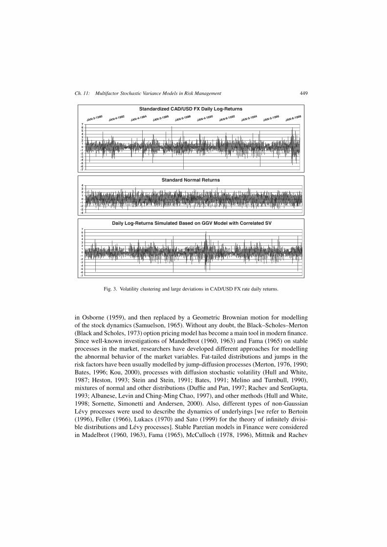
There is extensive empirical evidence that historical daily return distributions for differentunderlyings in the foreign exchange, interest rate, commodity, and equity markets havehigh peaks, “fat” tails (excess kurtosis, Figures 1 and 2) and skewness (right graph onFigure 2) contrary to the normal distribution [see, for example, Mandelbrot (1960), Fama(1965), Duffie and Pan (1997), Müller, Dacorogna and Pictet (1998), Barndorff-Nielsenand Shephard (2000b), Rachev and Mittnik (2000), Bouchaud and Potters (2000), Cont(2001)]. Also, it is well known that the volatility of these financial variables varies sto-chastically with clustering (Bollerslev, Engle and Nelson, 1994) (see Figure 3). These dis-tributional properties have significant impact on Risk Management, specifically on VaR.A standard methodology usually used for the VaR calculation (JP Morgan, 1996) exploitsa multivariate normal distribution as a proxy for the RF distributions. The standard modelcorresponds to stable market conditions when one can neglect large jumps of the under-lyings and volatility fluctuations. This results in underestimating of the actual VaR by thestandard methodology and breaching the back-testing. A comprehensive RF simulationmodel should additionally capture the following important features observed in the mar-ket:– different distributional shapes for different risk factors and markets (for example, short

interest rates have much heavier tails, higher peaks and kurtosis than long term rates evenfor the same interest rate curve, Figure 1; some commodity price distributions deviatemore from normal than others);

– anomalously small normalization effect for large diversified portfolios contrary to theone predicted by the Central Limit Theorem (for example, S&P 500 Industrial Indexor TSE 300 Index (Figure 2), viewed as large portfolios of stocks, have markedly non-normal distributions with kurtosis about ten). This phenomenon points to a non-lineardependence between different risk factors [see also Embrechts, McNeil and Straumann(1999)];

– normalization of the risk factor distributions for longer holding periods [for example,ten-day return distributions are significantly closer to normal than daily return distribu-tions, on the other hand, intraday change distributions are clearly more distant from nor-mal than daily ones (Müller, Dacorogna and Pictet, 1998; Cont, Potters and Bouchaud,1997; Mantegna and Stanley, 2000)]. A decreasing term structure of kurtosis points outto the same effect (Duffie and Pan, 1997; Bouchaud and Potters, 2000);

– volatility clustering and non-linear time dependence in risk factor returns (for example,statistically significant autocorrelation in squares of virtually uncorrelated daily returns,see top graph on Figure 3 and Figure 10 in Section 2.3).


Fig. 1. Variety of distributional shapes for CAD BA interest rate daily returns.

Fig. 2. Distributions for the CAD/USD FX and TSE 300 daily log-returns.

1.3. A short review of stochastic volatility models

In this chapter we restrict consideration of the SV models to the case of continuous timemodels. Time series approaches (ARCH, GARCH, etc.) (Bollerslev, 1986; Bollerslev, En-gle and Nelson, 1994) are beyond the scope of the chapter.

L. Bachelier introduced the normal distribution and Brownian motion in finance in hisPh.D. Thesis (Bachelier, 1900) more than one hundred years ago. Brownian motion [thatcorresponds to a standard model for VaR (JP Morgan, 1996)] was rediscovered in finance


Fig. 3. Volatility clustering and large deviations in CAD/USD FX rate daily returns.

in Osborne (1959), and then replaced by a Geometric Brownian motion for modellingof the stock dynamics (Samuelson, 1965). Without any doubt, the Black–Scholes–Merton(Black and Scholes, 1973) option pricing model has become a main tool in modern finance.Since well-known investigations of Mandelbrot (1960, 1963) and Fama (1965) on stableprocesses in the market, researchers have developed different approaches for modellingthe abnormal behavior of the market variables. Fat-tailed distributions and jumps in therisk factors have been usually modelled by jump-diffusion processes (Merton, 1976, 1990;Bates, 1996; Kou, 2000), processes with diffusion stochastic volatility (Hull and White,1987; Heston, 1993; Stein and Stein, 1991; Bates, 1991; Melino and Turnbull, 1990),mixtures of normal and other distributions (Duffie and Pan, 1997; Rachev and SenGupta,1993; Albanese, Levin and Ching-Ming Chao, 1997), and other methods (Hull and White,1998; Sornette, Simonetti and Andersen, 2000). Also, different types of non-GaussianLévy processes were used to describe the dynamics of underlyings [we refer to Bertoin(1996), Feller (1966), Lukacs (1970) and Sato (1999) for the theory of infinitely divisi-ble distributions and Lévy processes]. Stable Paretian models in Finance were consideredin Madelbrot (1960, 1963), Fama (1965), McCulloch (1978, 1996), Mittnik and Rachev


(1989), Willinger, Taqqu and Teverovsky (1999), Rachev and Mittnik (2000), and otherworks [see also Samorodnitsky and Taqqu (1994), Janicki and Weron (1994), Nolan (1998)for the theory, simulation and estimation of stable processes]. Since pioneering 1973 paperof Clark (1973), there have been a lot of research works on subordinated Lévy processes infinance: VG model (Madan and Seneta, 1990; Madan and Milne, 1991; Madan, 1999); Hy-perbolic and Generalized Hyperbolic models (Barndorff-Nielsen, 1977, 1978, 1997, 1998;Eberlein and Keller, 1995; Embrechts, McNeil and Straumann, 1999; Eberlein and Raible,1999) [see also Marinelli, Rachev and Roll (1999), Rachev and Mittnik (2000)]. A finestructure of asset returns from a Lévy process point of view was considered in Carr etal. (2000), Geman, Madan and Yor (1999, 1998) (CGMY model), Mantegna and Stanley(2000), Bouchaud and Potters (2000), Boyarchenko and Levendorskii (2000), Barndorff-Nielsen and Levendorskii (2001) (Truncated Lévy Flight). A general theory of condition-ally normal stochastic variance and stochastic time change models is considered in Steu-tel (1970, 1973), Rosinski (1991), Maejima and Rosinski (2000), Barndorff-Nielsen andPérez-Abreu (2000).

Most papers discuss a one-dimensional case with applications to option pricing. How-ever, multidimensional models with a large number of risk factors are of significance forRisk Management. This chapter presents a new class of multivariate VaR models with theSV driven by Lévy processes.

2. Single-factor stochastic variance model

2.1. Maximum entropy approach and Lévy processes

Let a risk factor X denote a t-day absolute return, relative return, or log-return of the under-lying market variable. Value-at-Risk over a given holding period t with a specified confi-dence level q (usually, q = 1%) is defined as a q-quantile of the distribution for the portfo-lio changes during the period t . For the standard model, a RF probability density functionis normal with given constant mean and variance. We consider a class of conditional nor-mal models where the variance V of the risk factor X is stochastic rather than constant.The stochastic variance of the underlying returns is not directly observable in the market.Generally, the most reliable information about the SV is its average value over some periodof time. It can be estimated from the sampling variance of the underlying returns. Underconditions of uncertainty, it is reasonable to adopt a conservative approach, i.e., choose aprobability distribution for the SV that provides the most uncertain outcomes given onlyinformation about the average value. A well-known measure of uncertainty associated withprobability distributions is entropy (Kagan, Linnik and Rao, 1973). Therefore, it is reason-able to determine the SV distribution from the Maximum Entropy principle.

A proposed single-factor SV model is based on the following assumptions (Levin andTchernitser, 1999a):


Assumption 1. The density function, pX(x,T ), of the risk factor X = X(T ) for someholding period T is normal conditional upon the stochastic variance V = V (T ) that pos-sesses a probability density function pV (v,T ), v � 0, i.e.,

pX(x,T ) =∫ ∞

0

1√2πv

exp

(− (x − θv −µT )2

2v

)pV (v,T )dv. (1)

Parameter µT specifies a constant part of the mean for the conditional normal distri-bution, and parameter θ defines a shift in the mean proportional to the SV. As is shownlater, θ determines the correlation between the RF and SV that results in a skewed RFdistribution. The case θ = 0 corresponds to a symmetric distribution. Linear dependence ofthe shift term θv from v in the mean of normal density is important for further constructionof a Lévy process for the RF. The stochastic representation for X is as follows:

X(T ) =√V (T )Z + θV (T ) +µT, Z ∼ N(0,1), (2)

with Z being a standard normal random variable independent of V (T ).

Assumption 2. The average variance E{V (T )} for the holding period T is known andequal to V :

E{V (T )

}=∫ ∞

0vpV (v,T )dv = V . (3)

Assumption 3. The probability density function pV (v,T ) of the stochastic variance V (T )

is defined by the Maximum Entropy principle given the average variance (3):

H(pV ) = −∫ ∞

0pV (v) lnpV (v)dv → max

pV (v)�0. (4)

The optimization problem (4) for the SV density pV (v) subject to the constraint onthe average variance (3) and standard normalization constraint

∫∞0 pV (v)dv = 1 has the

exponential density

pV (v) = 1V exp

(− v

V)

as a solution calculated by the Lagrange multiplier method (Kagan, Linnik and Rao, 1973).According to the Law of Total Probability, the unconditional density (1) of the risk factorX(T ) has the following density:

pX(x,T ) = λ

V exp

(−|x −µT |

λ+ θ(x −µT )

), λ =

√V

2 + θ2 V . (5)


Distribution (5) is known as the skewed double exponential (Laplace) distribution (Kotz,Kozubowski and Podgórski, 2001). This distribution has a sharp peak, exponential tails andnon-zero skewness for θ = 0. Kurtosis of a symmetric Laplace distribution is always equalto 6, in contrast to 3 for a normal distribution. Historical distributions of daily returns formany market variables, such as CAD/USD FX rate (Figure 2), JPY/USD FX rate, S&P 500Index, TSE 300 Index (Figure 2), NYMEX Natural Gas futures prices, some LIBOR rates,etc., have a similar leptokurtic shape (Levin and Tchernitser, 1999a; Kotz, Kozubowskiand Podgórski, 2001).

In the case of a linear portfolio and symmetric Laplace distribution for the RF, the impactof non-normality on VaR can be estimated as

VaRLaplace

VaRNormal= ln(2q)√

2zq,

where zq is a standardized normal quantile for the confidence level q . For the case q = 1%(zq = 2.3263), VaRLaplace for a linear portfolio is 19% higher than the standard VaRNormal.The impact on VaR is even more pronounced for non-linear instruments. For example, fora non-linear perfectly delta-hedged option portfolio, Π(x), within Delta–Gamma approx-imation for the portfolio changes, δΠ(x) = 0.5Γ x2, the corresponding formulas for VaRare as follows:

VaRLaplace = −V Γ

4ln2(q), VaRNormal = −V Γ

2(zq/2)

2.

This results in 60% higher VaRLaplace number than VaRNormal (Levin and Tchernitser,1999a).

The exponential distribution for the SV was derived from the Maximum Entropy princi-ple for some unspecified holding period T . To calculate VaR for different holding periods t ,a stochastic process for the risk factor X is required. The standard normal model assumesthat the risk factor X follows a Wiener process with independent stationary Gaussian incre-ments. The simplest extension of this assumption is that the RF follows a Lévy process, i.e.,a stochastic process with independent stationary (not necessarily Gaussian) increments. Itcan be shown (Rosinski, 1991) that within the class of conditionally normal models (2) thisassumption is equivalent to the following assumption on the SV:

Assumption 4. The total stochastic variance V (t) in (2) follows a positive increasing Lévyprocess.

The exponential distribution for the V (T ) is infinitely divisible. It uniquely determinesa positive increasing pure jump Gamma process [see Sato (1999)] for the total stochasticvariance V (t), t > 0, with a Gamma probability density function

pV (t)(v) = vαt−1

�(αt)βαtexp

(− v

β

), (6)


where α = 1/T , β = V . Assumptions 1–4 define the corresponding Lévy process for therisk factor X(t) with the following probability density function:

pX(x, t) =√

2

π

λ2αt−1 exp(θλy)

�(αt)βαt|y|αt−1/2Kαt−1/2

(|y|), y = x −µt

λ. (7)

Here λ is defined in (5), �(ν) is a gamma function, and Kν(y) is a modified Bessel functionof the third kind of the order ν, K−ν(y) = Kν(y) (Abramowitz and Stegun, 1972). Distri-bution (7) is known as a Bessel K-function distribution (Johnson, Kotz and Balakrishnan,1994) or as a Generalized Laplace distribution (Kotz, Kozubowski and Podgórski, 2001).Essentially, the SV model derived from the Maximum Entropy principle is equivalent tothe Variance Gamma (VG) model [Gamma stochastic time change model, see Madan andSeneta (1990), Madan and Milne (1991), Geman and Ané (1996)]. The tail asymptotic be-havior and behavior at the origin for the density (7) follows from known asymptotics forthe modified Bessel function Kν(y) (Abramowitz and Stegun, 1972)

Kν(y) ∼y→∞

√π

2ye−y, Kν(y) ∼

y→0�(ν)2ν−1y−ν, ν > 0, K0(y) ∼

y→0− ln(y).

The RF density (7) has exponential tails for all t and a wide range of shapes at the origin,from almost normal “bell” shape (for large α � 1) to a highly peaked (0.5 < α � 1) andeven unbounded shape (0 < α � 0.5) (see Figure 4). A skewed Laplace density (5) is aspecial case of (7) for t = T . The Bessel K-function family of distributions possessesfinite moments of all orders. The characteristic function for the Gamma process has asimple form

Fig. 4. Probability densities for the Gamma SV model.


φX(t)(ω) = E{eiωX(t)

}= exp(iωµt)

(1 − iωβθ +ω2β/2)αt. (8)

The Lévy density from the Lévy–Khintchine representation of φX(t)(ω) that characterizesthe intensity of jumps of different sizes x has the following closed form [see Sato (1999)]:

k(x) = α

|x| exp

(−√

2

β+ θ2|x| + θx

).

The RF distribution (7) tends to a normal distribution for t → +∞. This normalizationeffect is important for a proper VaR scaling from short holding periods to longer ones.The total variance DX(t) is proportional to time, as it is for any Lévy process with finitevariance (Feller, 1966) (a “square root of time” rule for the volatility is valid). However,contrary to the Gaussian case, the ratios of q-quantiles and standard deviation for the RFdistributions (7) are not constant for different holding periods t . For example, the standard-ized 1%-quantile (VaRVG) is higher for shorter holding period than the same 1%-quantilefor longer holding period (Figure 5).

The entropy for the SV distribution standardized by time t (the mean of a standardizedSV is equal to 1 for all t) has the maximum at t = T (Figure 6) that corresponds to theexponential distribution. This property may be explained by transition of the standardizedGamma density from the delta-function at 0 to the delta-function at 1 as time t passes.Heuristically, this evolution of shape for the SV density corresponds to a transition fromthe state of maximum certainty at time 0 to the limiting state of maximum certainty att = ∞ (with the limiting normal density for the standardized RF).

The following expressions provide a connection between the first four moments of theRF distribution and those of the SV distribution (Levin and Tchernitser, 2000a):

mX(t) = µt + θmV (t),

DX(t) = mV (t) + θ2DV (t),

(9)m3,X(t) = θ

(3DV (t) + θ2m3,V (t)

),

m4,X(t) = 3m2V (t) + 3DV (t) + 6θ2mV (t)DV (t) + 6θ2m3,V (t) + θ4m4,V (t).

Fig. 5. VG model 1%-VaR term structure with respect to 1% Normal VaR = 2.33.


Fig. 6. Evolution of standardized Gamma SV density and entropy.

The expressions (9) for the moments are valid for conditional normal models of the form(1) provided that the distribution pV (t)(v) for the stochastic variance V (t) possesses mo-ments up to the fourth order. Parameter θ controls skewness of the RF distribution anddefines the correlation ρX,V between the risk factor X and its stochastic variance V :

ρX,V = θ

√DV

mV + θ2DV

.

A parameter estimation procedure (model calibration), with respect to the four para-meters, µ, θ , β , and α can be based either on the Maximum Likelihood approach or themethod of moments given four sampling central moments for the T1-day underlying returnsand analytical expressions for the moments of the Gamma stochastic variance (Johnson,Kotz and Balakrishnan, 1994)

mV(T1) = αT1β, DV (T1) = αT1β2,

m3,V (T1) = 2αT1β3, m4,V (T1) = 3αT1β

4(αT1 + 2).

Equations (9) can be used for the model calibration by the method of moments. Note thattime T , corresponding to the maximum entropy for the SV density, can be recovered fromthe calibrated parameter α as T = 1/α.

It follows from (6) and (9) that the term structure of the RF variance and kurtosis for thesymmetric case of the Gamma-SV model (θ = 0) is:

DX(t) = αβt, KurtX(t) − 3 = 3

αt. (10)


2.2. Generalized Gamma Variance model

Some market variables exhibit jumps as large as 5 to 10 daily standard deviations (Fama,1965; Bouchaud and Potters, 2000; Mantegna and Stanley, 2000; Cont, 2001). Such eventshave significantly lower theoretical probability to occur for the corresponding periods ofobservations not only for the normal model, but even for the Gamma SV model with expo-nential tails. Extremely large jumps in the risk factors have often been described by distri-butions with polynomial tails, specifically by stable distributions (Mandelbrot, 1960, 1963;Mittnik and Rachev, 1989, 2000). However, stable Paretian distributions do not have finitevariance (volatility). This contradicts the majority of empirical observations [see Müller,Dacorogna and Pictet (1998)]. Also, volatility is a main tool in financial risk managementand pricing. Therefore, heavy tailed distributions with finite variance are of considerableinterest for the finance applications. An example of such distribution widely discussed inthe financial literature is Student t-distribution (Platen, 1999; Albanese, Levin and Ching-Ming Chao, 1997; Rachev and Mittnik, 2000). A new family of the RF distributions intro-duced below includes t-distribution as a special case. The symmetric Gamma SV modelconsidered above has only one shape parameter, α, that controls both the tails and cen-tral part of the distribution. It seems that one shape parameter is insufficient to distinguishbetween sources of high kurtosis: whether it comes from heavy tails or high peak. It ispossible to show that for a class of conditional normal models the tail asymptotics of theRF distribution depends upon the tail asymptotics of the corresponding SV distribution.Therefore, a more general SV model that allows for separate control for the tails and peakshould more successfully describe large deviations of the risk factors.

Note, that the Gamma SV density (6) can be formally derived from the Maximum En-tropy principle (4) without Assumption 4. Instead, one can use a constraint on the logarith-mic moment E{ln(V )} in addition to the condition on the average variance E{V } (Kagan,Linnik and Rao, 1973). Essentially, this logarithmic constraint defines a power behaviorof the SV density at the origin, while the constraint on E{V } defines the exponential tailbehavior. The condition on average variance can be replaced by a more flexible conditionto accommodate information on a generalized moment of any power for the SV (Levinand Tchernitser, 2000a, b). For example, one can assume that the average volatility isknown instead of average variance. This approximately corresponds to a constraint on thefractional moment E{√V } instead of E{V }. Hence, we can formally define the entropymaximization problem (4) with two essential constraints

∫ ∞

0ln(v)pV (v)dv = c0,

∫ ∞

0v1/νpV (v)dv = c1 (11)

and a standard normalization constraint for a probability density function. The use ofthe Maximum Entropy approach with a constraint on the generalized moment E{V 1/ν},ν ∈ R

1, allows for a desirable generalization of the Gamma SV model to a broad class ofmodels with a wide range of heavy tails, from exponential and sub-exponential (stretched


exponential) to polynomial (Levin and Tchernitser, 2000a, b). A solution of the maximiza-tion problem (4), (11) is the Generalized Gamma density for the stochastic variance V :

pV (v) = vα/ν−1

|ν|�(α)βαexp

(−v1/ν

β

). (12)

The corresponding stochastic representation for V is a ν-th power of the Gamma distrib-uted random variable γ with the density (6) [see Johnson, Kotz and Balakrishnan (1994)]:

V = γ ν. (13)

Stochastic representations (2) and (13) allow for an effective Monte Carlo simulation pro-cedure for the RF given well-known simulation procedures for normal and gamma randomvariables (Fishman, 1996).

The Generalized Gamma distribution is a very flexible class of distributions with twoshape parameters α and ν. This class includes Gamma (ν = 1), Inverse Gamma (ν = −1),and Weibull (α = 1, ν > 0) distributions as special cases. It is known that the GeneralizedGamma distribution is infinitely divisible for these three representatives [see Grosswald(1976), Ismail (1977), Sato (1999)] and for positive ν � max(α,1) (Ismail and Kelker,1979). Therefore, for these cases the Generalized Gamma distribution produces Lévyprocesses for the SV. We do not know if the Generalized Gamma distribution is infinitelydivisible for arbitrary values of ν ∈ R

1, nor whether there is a closed form representationfor the characteristic function. Hence, we apply the distribution (12) to describe the returnsfor the shortest holding period available, say one day, and then construct an additive SVprocess for a longer holding period, say 10 days, by summing up the independent Gener-alized Gamma distributed random variables. An analytical formula for the moments of theGeneralized Gamma distribution is readily available

E{V k}= βkν�(α + kν)

�(α)

(the condition for the k-moments to exist is (α + kν) > 0).The corresponding RF density pX(x) is given by the integral (1) with SV density pV (v)

being of the form (12). We call this density a Generalized Gamma Variance density (GGV).Unfortunately, in the general case there is no closed analytical form for the density pX(x).However, we consider an effective numerical procedure for calculating the integral (1) to beas good as, for example, a “closed form” formula (7) involving special K-Bessel functions.Effective asymptotic expansion methods (Olver, 1974; Abramowitz and Stegun, 1972) canbe applied for the numerical calculations.1 In the case of a symmetric GGV density, thereis an analytical formula for the moments of any fractional order k (finite for α+kν/2 > 0):

1 Effective numerical procedure and software for the GGV density calculation was developed by Xiaofang Ma.


E{|X|k}= 2k/2βkν/2�((k + 1)/2)�(α + kν/2)√

π�(α). (14)

The moments cease to exist for some combinations of negative values of ν and α > 0because of polynomial tails for the GGV density.

Below, we provide some results for a symmetric density pX(x). There are some knownspecial analytical cases for pX(x):

(i) ν = −1 corresponds to the t-distribution with 2α degrees of freedom;(ii) ν = 0 corresponds to the Gaussian distribution;

(iii) ν = +1 corresponds to the K-Bessel function distribution (7).Table 1 presents a summary of results for the Generalized Gamma Variance model,

including a constraint on the generalized moment in Maximum Entropy principle (col-umn 1), SV stochastic representation (column 2), corresponding RF density (column 3),and asymptotics for the tails of the RF density (column 4).

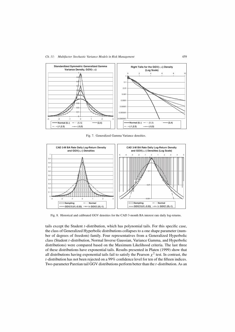
Some market variables are better described by distributions with polynomial tails, whileothers are better described by distributions with semi-heavy tails (exponential and sub-exponential) [see Platen (1999), Rachev and Mittnik (2000), Duffie and Pan (1997)]. TheGGV model is capable of accommodating both types of behavior. A range of values ν < 0corresponds to a power low tails. GGV density is finite at zero for all ν < 0. A range ofvalues ν > 0 corresponds to exponential and sub-exponential tails. In this case, tails arefar lighter and the moments of all orders exist. The range ν > 1 corresponds to a classof stretched exponential densities pX(x). The specific class of the stretched exponentialdistributions based on a modified Weibull density was considered in Sornette, Simonettiand Andersen (2000). Figure 7 shows the RF GGV density pX(x) for different values ofparameters ν and α. Parameter ν brings an extra flexibility to the GGV density: it is seenthat GGV model can accommodate a wide variety of shapes and tail behavior.

A statistical investigation of different SV models from a Generalized Hyperbolic familybased on historical data for 15 stock market indices was presented in the paper by Platen(1999). The class of Generalized Hyperbolic distributions developed in Barndorff-Nielsen(1978, 1998), Eberlein and Keller (1995), Eberlein, Keller and Prause (1998) is also a twoshape parameter family in symmetric case. All members of this family have exponential

Table 1GGV model summary

Constr. E{V 1/ν} SV density & Stoch. rep. RF density RF asymptotics x → ∞E{V }, ν = 1 Gamma, V = γ K-Bessel ∼xα−1 e−cx

E{√V }, ν = 2 Square of Gamma, V = γ 2 GGV(2, α) ∼x2α/3−1 e−cx2/3

E{1/V }, ν = −1 Inverse Gamma, V = 1/γ t-Distribution ∼x−(2α+1)

E{V 1/ν}, ν > 0 Generalized Gamma, V = γ ν GGV(ν,α) ∼x2α/(1+ν)−1 e−cx2/(1+ν)

E{V 1/ν}, ν < 0 Generalized (Inv.) Gamma, V = γ ν GGV(ν,α) ∼x−(2α/|ν|+1)

ν = 0 SV degenerates to V ≡ 1 Normal ∼e−x2/2


Fig. 7. Generalized Gamma Variance densities.

Fig. 8. Historical and calibrated GGV densities for the CAD 3-month BA interest rate daily log-returns.

tails except the Student t-distribution, which has polynomial tails. For this specific case,the class of Generalized Hyperbolic distributions collapses to a one shape parameter (num-ber of degrees of freedom) family. Four representatives from a Generalized Hyperbolicclass (Student t-distribution, Normal Inverse Gaussian, Variance Gamma, and Hyperbolicdistributions) were compared based on the Maximum Likelihood criteria. The last threeof these distributions have exponential tails. Results presented in Platen (1999) show thatall distributions having exponential tails fail to satisfy the Pearson χ2 test. In contrast, thet-distribution has not been rejected on a 99% confidence level for ten of the fifteen indices.Two-parameter Paretian tail GGV distributions perform better than the t-distribution. As an


Fig. 9. GGV model log-likelihood surface for S&P 500.

example, Figure 8 demonstrates a fit for the Canadian 3-month BA interest rate daily returndensity (1992–1998) by normal, Student-t , and GGV densities calibrated using MaximumLikelihood approach. It is seen that GGV(α, ν) with optimal parameters ν = −5.5 andα = 15 outperforms t-distribution, and both GGV and t-distributions significantly outper-form normal. The χ2 value for the GGV(15,−5.5) is about 80% less than χ2 value for thecalibrated t-distribution. It is interesting to note, that during the period 1992–1998, Cana-dian 3-month BA interest rate exhibited 14 large daily moves greater than four standarddeviations (about 1% of all observations).

Another example (Figure 9) shows a GGV model log-likelihood surface for S&P 500Index as a function of parameters ν and α. A deep minimum for ν = 0 corresponds to thenormal distribution, while two wings correspond to the power law (ν < 0) and stretchedexponential (ν > 1) tailed distributions. For this example, a stretched exponential sub-classproduces almost the same maximum likelihood value as a power law sub-class.

2.3. Mean-reverting stochastic variance model

So far, we have considered a class of the SV models driven by Lévy processes with in-dependent, identically distributed, but not necessarily Gaussian increments. The modelexplains non-normality of the RF distributions. For any conditional normal SV model, ex-pressions (9) provide an exact answer for the term structures of the risk factor variance andkurtosis


DX(t) = mV (t), KurtX(t) − 3 = 3DV (t)

m2V (t)

. (15)

Here V (t) is a total variance. Since mV(t) and DV (t) are linear functions of time for anyLévy process for V (t), the above expressions predict linear increase of the RF varianceand hyperbolic decrease of its excess kurtosis.

However, empirical investigations show that the underlying returns are almost uncor-related, but not independent [see Bouchaud and Potters (2000), Cont (2001), Müller, Da-corogna and Pictet (1998)]. The easiest way to demonstrate this dependence is to considerthe empirical correlations for the absolute values or squares of the returns. It is seen (Fig-ure 10) that autocorrelations of squares are statistically significant. This phenomenon isconnected with a known volatility clustering effect (Figure 3). Also, it is known that em-pirical term structure of kurtosis decreases slower than is predicted by a “Lévy term struc-ture” model (15) [so called “anomalous decay”, see Bouchaud and Potters (2000), Cont(2001)]. All this suggests that a better model for the instantaneous stochastic volatility isnot a “white noise” kind of process, but rather a process with autocorrelation. One wayto account for the autocorrelation structure of the SV is to consider regime-switching SVprocesses [see Konikov and Madan (2000)]. We will follow another approach to intro-duce the SV autocorrelation by considering Ornstein–Uhlenbeck (OU) type processes forthe instantaneous SV (Levin and Tchernitser, 1999a, 2000a). Such class of non-GaussianOU type processes driven by positive Lévy noise was investigated in detail in Barndorff-Nielsen and Shephard (2000a, b). In this section we will only demonstrate that the empir-ically observed term structure of kurtosis can be consistently described by such models.

Consider a stationary non-negative process ξ(t) with autocorrelation function Rξ (τ) thatdescribes the instantaneous stochastic variance. For the total variance V (t) being V (t) =∫ t

0 ξ(t ′)dt ′, it follows that

mV(t) = mV (1)t, DV (t) = 2∫ t

0(t − τ )Rξ (τ )dτ.

The above expressions in conjunction with (15) can be used to calculate a term structureof the RF kurtosis. In particular, assume a mean-reverting process for the instantaneousstochastic variance ξ(t) be a Ornstein–Uhlenbeck type process

dξ(t) = −λξ(t)dt + λdG(t), (16)

where G(t) is, for example, a Gamma process, λ > 0 is a mean-reversion speed parameter.Expressions for Rξ (τ) and variance DV (t) are as follows

Rξ (τ) = λαβ2

2e−λ|τ |, DV (t) = αβ2t

2

(1 − 1 − e−λt

λt

).


Fig. 10. Autocorrelation in the squared CAD/USD FX daily returns and in the SV.

The autocorrelation function Rξ (τ) is an exponential function for any OU model (16). Itis seen that DV (t) is not a linear function of time contrary to the Lévy case (10). Previousformulas and formulas (15) result in the following term structure of the RF kurtosis:

KurtOUX(t) − 3 = 3

αt

(1 − 1 − e−λt

λt

).

Figure 11 shows a term structure of the RF kurtosis for different values of the mean-reversion speed parameter λ. As expected, the OU stochastic variance process provides


Fig. 11. Term structure of the RF kurtosis for the model with autocorrelated SV.

slower decay of kurtosis vs. Lévy SV process. Reduction in decay can be significant de-pending upon the mean-reversion speed λ. This is equivalent to slower “normalization”effect. The bottom graph in Figure 10 presents the time series for the simulated SV andempirical CAD/USD FX rate squared daily log-returns. The bottom graph in Figure 3presents the simulated RF time series. It is evident that the model produces large devia-tions for the FX rate and volatility clustering effect that is very similar to the one observedin the market (top graph in Figure 3).

3. Multifactor stochastic variance model

3.1. Requirements for multifactor VaR models

A realistic multifactor VaR model should consistently describe not only the correlation andvolatility structure for the risk factors, but also different shapes of the marginal risk fac-tor distributions and distributions in other “diagonal” directions. Also, a principal compo-nent analysis for daily returns in different markets (interest rate curves, commodity futuresprices, implied volatility curves and surfaces), clearly indicates the presence of non-lineardependence between risk factors (principal components). For example, the squared dailychanges of the principal components are significantly correlated, while daily changes them-selves are uncorrelated. This non-linear dependence breaks conditions of the Central LimitTheorem and has an important impact on VaR calculation: even for well-diversified linearportfolios with a large number of instruments there is no full normalization of the portfolioreturn distributions (Levin and Tchernitser, 1999a, b). An example of such large diversi-fied portfolio is the S&P 500 Index. Its distribution is quite far from normal despite theportfolio averaging effect. Hence, a comprehensive model for multiple risk factors shouldadditionally capture the following important features observed in the market:


• exact match of a given volatility and correlation structure of the risk factors;• approximate match of shapes, kurtosis, and tails for different risk factors (marginal dis-

tributions);• approximate match of shapes, kurtosis, and tails for different linear sub-portfolios (mar-

ginal distributions in diagonal directions).The model should also allow for an effective Monte Carlo simulation procedure. To facil-itate further multivariate analysis, in the sequel, we shall consider the case of symmetricjoint probability distributions for the RF returns.

3.2. “Naïve” multifactor model

A very simple idea for constructing a multivariate conditionally Gaussian stochastic vari-ance model is to define a distribution for the vector of risk factors X(t) ∈ R

N as a multi-variate normal with some fixed correlation matrix R and independent stochastic variancesVi(t), i = 1, . . . ,N . A symmetric multivariate probability density function for the vectorof risk factors is represented as:

pX(t)(x) =∫V1

· · ·∫VN

1√(2π)N det(C)

× exp

(−x ′C−1x

2

)pV (V1, . . . , VN)dV1 · · ·dVN, (17)

C = ΣRΣ ′, Σ = diag(√

V1(t), . . . ,√VN(t)

). (18)

Here pV (V1, . . . , VN) =∏Ni=1 pVi (Vi) is a probability density for independent stochas-

tic variances Vi(t), x ′ is transpose of x . The corresponding stochastic representation forthe risk factors X(t) is

X(t) = diag(√

V1(t), . . . ,√VN(t)

)AZ, AA′ = C, Z ∼ N(0, I ), (19)

where Z ∼ N(0, I ) is independent of V standard normal vector with identity covariancematrix I. This representation allows for modelling marginal distributions with differentleptokurtic shapes.

However, it can be shown that this “naïve” approach reduces the correlations betweenrisk factors because of “randomization” for the covariance matrix (Levin and Tchernitser,1999a). Due to independence of the stochastic variances Vi , absolute values of the modelcorrelations Corr(Xi,Xj ) are less than absolute values of the correlations Rij used in (17):

Cov(Xi,Xj ) =∫ ∫

xixjpX(x)dxi dxj = Rij

∫ ∫ √Vi

√VjpV (Vi,Vj )dVi dVj

= Rij

∫ √VipVi (Vi)dVi

∫ √VjpVj (Vj )dVj

= fij σX,iσX,jRij , i = j. (20)


Table 2Correlation reduction factors

αi = αj 0.5 1 2 5 10f (αi ,αj ) 0.64 0.79 0.88 0.95 0.98

Reduction factors fij , i = j , are less than one, because

∫ √Vi1pVi (Vi)dVi <

√∫VipVi (Vi)dVi

√∫1pVi (Vi)dVi =√

E{Vi} = σX,i .

It means that the sampling correlation matrix cannot be used as the matrix R in (17).For example, the reduction factors fij < 1, i = j, calculated explicitly for the case of theGamma stochastic variances (6) are as follows:

Corr(Xi,Xj ) = fijRij , fij = f (αi, αj ) = �(αi + 1/2)�(αj + 1/2)

�(αi)�(αj )√αiαj

, i = j.

The underestimation of the correlations can be significant for some values of parametersαi , αj as it is shown in Table 2.

The randomization effect exists for any probability density functions pVi (Vi) for inde-pendent stochastic variances. Usually, equations Corr(Xi, Xj ) = fijRij cannot be resolvedwith respect to correlations Rij given sampling correlations Corr(Xi, Xj ) while preservingthe necessary conditions |Rij | � 1 or non-negative definite matrices R. Hence, this “naïve”model does not allow to preserve historical correlations between the risk factors.

Remark. Equation (20) and the inequality∫ ∫ √Vi

√VjpV (Vi,Vj )dVi dVj <

√Cov(Vi,Vj )+E{Vi}E{Vj }

imply that the class of the SV models with the stochastic representation (18) for the covari-ance matrix preserves the RF correlation structure only if∫ ∫ √

Vi

√VjpV (Vi,Vj )dVi dVj =√

E{Vi}√E{Vj },

which requires dependent stochastic variances with positive correlations. We do not inves-tigate this direction in the chapter.

3.3. Elliptical stochastic variance model

The simplest extension of a single-factor SV model to the multifactor case is an ellip-tical stochastic variance model. Elliptical models are widely used for representing non-


normal multivariate distributions in finance [see Eberlein, Keller and Prause (1998), Kotz,Kozubowski and Podgórski (2001)]. This class of models preserves the observed RF cor-relation structure. The model is similar by construction to the one-dimensional variancemixture of normals. An elliptical N -dimensional symmetric process XE(t) for N risk fac-tors has a stochastic representation as a single variance mixture of multivariate normalswith a given covariance matrix C:

XE(t) =√V (t)ZC, ZC ∼ N(0,C). (21)

Here V (t) is a univariate SV process, ZC is a multivariate normal N -dimensional vec-tor independent of V (t). The covariance matrix C is estimated from historical T1-day re-turns (e.g., daily returns), while the SV is normalized to satisfy a condition mV (T1) =E{V (T1)} = 1. The unconditional density for the random vector of risk factors XE(t) is:

pXE(t)(x) =∫ ∞

0

1√(2πV )N det(C)

exp

(−x ′C−1x

2V

)pV (t)(V )dV.

As an example, consider the case of Gamma stochastic variance V (t). A closed analyt-ical form for the unconditional elliptical Bessel K-function density for XE(T ) is availablein Kotz, Kozubowski and Podgórski (2001). A characteristic function φXE(t)(ω) for theelliptical Lévy process XE(t) is represented as:

φXE(t)(ω) =(

1 + β

2ω′Cω

)−αt

, (22)

where ω is N -dimensional vector, ω′ is a vector transposed to ω. Due to known propertiesof elliptical distributions [see Fang, Kotz and Ng (1990)], all marginal one-dimensionaldistributions for the risk factors are univariate Bessel K-function distributions with thesame shape parameter αt and the same kurtosis. They differ only by the standard de-viations. The same property holds for all one-dimensional distributions of linear combi-nations X∆ = ∆′XE(t) of the risk factors. These linear combinations correspond to thelinear portfolios defined by ∆. The kurtosis of X∆(T1) for any arbitrary ∆ is equal tok∆ = 3(1 + DV (T1)/m

2V (T1)) = 3(1 + DV (T1)). Therefore, within the class of elliptical

models there is no normalization effect at all for the distributions of large diversified port-folios. This is a result of violation of the conditions for the Central Limit Theorem: therisk factors are dependent through the common stochastic variance V . Such property is adrawback for all elliptical models. It is clear that the actual RF fluctuations are not drivenby a single stochastic variance (“global market activity”). More realistic SV model shouldinclude a multidimensional processes for the SV to model different distributional shapesfor the risk factors and linear sub-portfolios. Since sampling marginal RF distributionshave different shapes, the calibration of elliptical model is restricted to fitting a distribu-tion of some preselected portfolio. Hence, the calibration of elliptical models is portfoliodependent.


3.4. Independent stochastic variances for the principal components

One of the possible ways to model different shapes for the RF distributions while preserv-ing a given correlation structure was considered in Levin and Tchernitser (1999a, b). AnN -dimensional vector of the risk factors is represented as a linear combination of principalcomponents (PC) with independent one-dimensional stochastic variances. The correspond-ing stochastic representation is as follows:

XL(t) = AZI (t), ZIi (t) =√

Vi(t)Zi, Zi ∼ N(0,1), i = 1, . . . ,M.

Here Zi are independent standard normal variables, Vi(t) are independent SV processeswith a unit mean and some variances DV i for a specified time horizon T1. The columnsof a constant matrix A are the principal components of a given covariance matrix C. Thecovariance matrix C is estimated from the historical T1-day returns. Matrix A is calculatedbased on eigenvalue decomposition of the covariance matrix C [see Wilkinson and Reinsch(1971)]:

C = UDU ′, U ′ = U−1, D = diag(d1, . . . , dN), (23)

A = UMD1/2M , DM = diag(d1, . . . , dM), M �N, C = AA′. (24)

Matrix UM consists of the first M columns of the orthogonal matrix U , which correspondto the first M largest eigenvalues d1, . . . , dM of the matrix C. Number M may be chosenless than N if the matrix C is singular and has only M non-zero eigenvalues. Some numer-ical issues related to singularity of the matrix C were considered in Kreinin and Levin(2000). It follows from the construction of the process XL(t) that Cov(XL(T1)) = C. Thisensures an exact match of the sampling covariance matrix C. One can keep even a smallernumber M of the principal components in (24) and recover the matrix C with the requiredaccuracy.

A characteristic function for the model is a product of the characteristic functions of one-dimensional processes for the PCs. For example, a characteristic function for the GammaSV model with independent SV has a form

φXE(t)(ω) =M∏i=1

(1 + (ω′(A)i)

2

2

)−αi t

,

where (A)i is i-th column of the matrix A.The matrix A can be defined up to an arbitrary orthogonal transformation H without

change of the covariance matrix C since Zi are independent standard normal variables, Zi

and Vi(T1) are independent and E{Vi(T1)} = 1. Hence, E{ZI(T1)ZI (T1)

′} = I and

E{XL(T1)X

L(T1)′}= AHE

{ZI(T1)Z

I (T1)′}H ′A′ = AHH−1A′ = C


for any orthogonal matrix H . However, the matrix H influences a matrix of the fourthmoments of XL(t), Kij = E{(XL)2

i (XL)2

j }. The orthogonal matrix H and shape param-eters for the Vi can be determined to approximate a given sampling matrix {Kij } of thefourth moments for the RF distribution (all moments E{(XL)3

i (XL)j } are equal to zero for

symmetric distributions). An explicit calculation yields:

Kij = E{(XL)2i

(XL)2j

}= 3M∑k=1

a2ika

2jkDV k +CiiCjj + 2C2

ij ,

i, j = 1, . . . ,N, (25)

where aik are the elements of the matrix A= AH . An effective method for calculating thematrix H and shape parameters is discussed in Section 3.6 below.

The model provides an exact match of the RF correlation and volatility structures andapproximates different shapes and kurtosis of the marginal RF distributions contrary tothe Elliptical model. However, there is a significant drawback for this model. Since thestochastic variances Vi are independent, there is a strong normalization effect in any “di-agonal” direction. This means that some linear portfolios X∆(t) = ∆′XL(t) have almostnormal distributions whenever the portfolio Delta, ∆, is not a marginal direction and thenumber of principal risk factors M is large enough. Described effect presents a real dan-ger, because the non-normal marginal RF distributions may be well-approximated, whilethe modelled portfolio distributions (contrary to the actual sampling distributions) may bealmost normalized and the VaR underestimated.

3.5. A model with correlated stochastic variances

As it was pointed out above, a more general and realistic market model should incorpo-rate the correlated stochastic variances that can correct the deficiencies of both Ellipticalmodel and the model with independent SV for the principal components. The correlated SVstructure should allow modeling of some general economic factors as well as idiosyncraticcomponents that drive the SV processes for different risk factors and markets.

The model is defined via stochastic representation of the following form (Levin andTchernitser, 2000a, b):

XCV (t) = AZI (t), ZIi (t) =√

Vi(t)Zi, Zi ∼ N(0,1), i = 1, . . . ,M. (26)

Here Zi are independent standard normal variables, Vi(t) are the correlated stochastic vari-ance processes with a unit mean for a specified time horizon T1. The matrix A ∈ R

N×M isdefined as in the previous section through the eigenvalue decomposition for the covariancematrix C up to an arbitrary orthogonal transformation H ∈ R

M×M :

C = Cov(XCV (T1)

)= AA′ = AA′, A = AH, H ′ = H−1.


Stochastic variances Vi(t) are correlated to each other due to the following stochastic rep-resentation:

Vi(t) =L∑

k=1

bikξk(t),

L∑k=1

bik = 1, bik � 0, B ∈ RM×L, (27)

where ξk(t) are independent positive increasing Lévy processes with unit mean for the timehorizon T1 and different shape parameters, and B is a constant matrix with non-negativeelements. The processes ξk(t) are the drivers for the SV processes Vi(t). For example, eachdriver ξk can be a Gamma process or Generalized Gamma process. Linear structure in (27)with bik � 0 ensures that Vi(t) are positive increasing Lévy processes. The normalizationconditions E{ξk(T1)} = 1 and

∑bik = 1 ensure, as in Section 3.4, exact recovering of the

sampling covariance matrix for the risk factors. It follows, that the vector of stochasticvariances V (T1) has covariance matrix CV equal to

CV = Cov(V (T1)

)= BDξB′,

Dξ = diag(Dξ1, . . . ,DξL), Dξk = Var{ξk(T1)

}. (28)

The multivariate Generalized Stochastic Variance (GSV) model (26), (27) has two lev-els of correlations. First level defines usual correlations across the risk factors described bythe covariance matrix C. Second level defines the correlations across the stochastic vari-ances described by the covariance matrix CV . The second level of correlations providesa possibility to obtain an approximate, but consistent match of the higher order momentsand shape of the RF multivariate distribution. The elliptical model and the model withindependent stochastic variances are the special cases of the above GSV model. Ellipti-cal model corresponds to the matrix B being equal to one column with all unit entries,B = [1, . . . ,1]′. The model with independent SV corresponds to the case when the matrixB is equal to the identity matrix, B = I .

There is no analytical form for the probability density function of the vector XCV (t)

even for the Gamma drivers ξk(t). However, a characteristic function φXCV (t)(ω) can becalculated as

φXCV (t)(ω) =∫ξ∈R

L+exp

(−1

2ω′Adiag(Bξ)A′ω

)pξ(t)(ξ)dξ

=L∏

j=1

∫ +∞

0exp

(−ξj

2

M∑i=1

bij

[N∑k=1

Akiωk

]2)pξj (t)(ξj )dξj .

The expression for the characteristic function above is equivalent to

φXCV (t)(ω) =L∏

j=1

∫ +∞

0exp

(−ξj

2ω′Cj ω

)pξj (t)(ξj )dξj ,


where Cj , j = 1, . . . ,L, are certain positive semi-definite matrices. The latter expressionfor the characteristic function allows for a different interpretation of the GSV model. Itshows that the process for the risk factors XCV (t) can be presented as a sum of L indepen-dent elliptical Lévy processes. In turn, each of these elliptical processes has a multivariateconditional normal distribution with a covariance matrix proportional to Cj and the corre-sponding stochastic variance ξj (t).

The kurtosis k∆ of a linear combination of the risk factors X∆(T1) = ∆′XCV (T1) forany given direction ∆ can be calculated analytically:

k∆ − 3 = E{X4∆(T1)}

E{X2∆(T1)}2

− 3 = 3η′CV η = 3η′BDξB′η,

η ∈ RM, ηk = (∆′A)2

k

‖∆′A‖2 , k = 1, . . . ,M. (29)

The above expression provides a link between the covariance matrix CV and the kurtosisk∆, that characterizes the shape of the RF multivariate distribution for the linear portfo-lio with Delta equal to ∆. Another useful quantity that clarifies the role of the correlatedvariances Vi is a standardized matrix of the fourth moments. This matrix, {kij }, is a multi-dimensional analog for kurtosis

kij = E{(XL)2i (X

L)2j }

E{(XL)2i }E{(XL)2

i }. (30)

The matrix {kij } incorporates kurtosis in all marginal and all pair-wise diagonal directionsin the original risk factor space. It is expressed as

kij − (1 + 2ρ2

ij

)=M∑k=1

M∑l=1

λ2ikλ

2j l Cov(VkVl) + 2

M∑k=1

M∑l=1

λikλjkλilλjl Cov(VkVl),

λik = aik

‖ai‖ , ‖ai‖2 =M∑k=1

a2ik, (31)

where ρij is a correlation between i-th and j -th risk factors. Formulas (29) and (31) clearlyindicate that the correlation structure of the SV is embedded into the correlation structureof the fourth moments of the RF distribution. This connection will be used as the basefor the GSV model calibration. A number L of the SV drivers can be chosen significantlysmaller than a number of stochastic variances M and risk factors N . These SV drivers maybe thought as “stochastic activities” for different countries, industries, sectors, etc.

The GSV model with the correlated stochastic variances is, in fact, a general framework.It can incorporate any reasonable processes to represent the SV drivers ξk(t), k = 1, . . . ,L.Some examples of suitable one-dimensional SV driver distributions are: Inverse Gaussian


distribution (Barndorff-Nielsen, 1997), Gamma distribution (Madan and Seneta, 1990;Levin and Tchernitser, 1999a), Lognormal distribution (Clark, 1973), or considered aboveclass of Generalized Gamma distributions. The GSV model is practical in terms of effec-tive Monte Carlo simulation: it is based on the simulation of one-dimensional SV processesand standard multivariate normal variables.

3.5.1. Example 1. Joint distribution for DEM/USD and JPY/USD FX rates

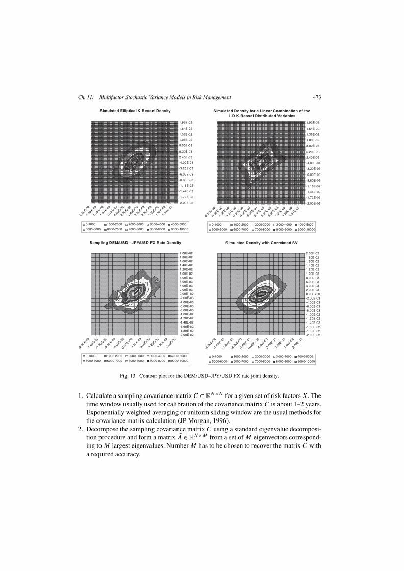
The first example presents a bivariate GSV model applied to the foreign exchange marketdata. Four bivariate models were examined for DEM/USD and JPY/USD FX rate dailyreturns: Standard Gaussian model, Elliptical Gamma Variance model, model with inde-pendent stochastic variances for PCs, and the model with correlated SV. Figures 12 and13 show a 3-D plot and a contour plot of the joint probability density for the historicaldata and four types of the models considered. All three SV models provide a far better fitthan the Gaussian distribution. However, the most convincing fit is provided by the GSVmodel with the correlated stochastic variances. Marginal distributions for DEM/USD andJPY/USD FX rates have kurtosis 5.2 and 6.9 respectively. Figures 14 and 15 show thatthe latter model is able to capture kurtosis and shape of marginal distributions in differentdirections.

3.5.2. Example 2. Twenty risk factors

The second example examines a 20-dimensional GSV model with correlated SV appliedto the data from the interest rate, FX rate, and equity markets. The USD and CAD zerointerest rate curves each consisting of nine interest rates, CAD/USD FX rate, and S&P 500Index were chosen as a representative set of the risk factors. There were 5 years (1994–1999) of daily historical data used for the model calibration (about 1,250 data points).Figure 16 presents statistical results for principal component analysis and the correlationmatrix for squares of the first three PCs. These results indicate that uncorrelated PCs neitherare normal nor independent. The first three “largest” PCs per zero curve were used for theGSV model calibration and simulation. Three Gamma distributed drivers ξk , k = 1,2,3,with different shape parameters were utilized to represent each stochastic variance Vi , i =1,2,3, for PCs. Therefore, the following values for parameters were assigned: number ofrisk factors N = 9×2+1+1 = 20, number of principal risk factors M = 3×2+1+1 = 8,number of SV drivers L = 3.

The model was calibrated to match kurtosis (in the least squares sense) for all 20 riskfactors and kurtosis for 15 additional linear sub-portfolios. Sampling kurtosis varies withina wide range from 5 to 25. Typically, kurtosis for short-term interest rates is much higherthan kurtosis for long-term rates. It is seen (Figure 17) that the GSV model reproducesthis typical decreasing kurtosis term structure quite well. It is also seen that the modeladequately matches kurtosis of the FX rate and S&P 500 Index, as well as kurtosis of dif-ferent linear sub-portfolios. To compare, the standard multi-dimensional Gaussian modelproduces a flat kurtosis term structure identically equal to three.


Fig. 12. Joint density for DEM/USD and JPY/USD FX rate.

3.6. Calibration for the GSV model

The GSV model is a two-level model that incorporates a traditional variance–covariancestructure of the risk factors and novel variance–covariance structure of the RF stochasticvariances. The GSV model with correlated SV automatically preserves the RF covariancematrix C. At the second level, it is necessary to calibrate the SV covariance matrix CV toapproximate the fourth moments of the multivariate RF distribution.

The main steps of the model calibration procedure are as follows:


Fig. 13. Contour plot for the DEM/USD–JPY/USD FX rate joint density.

1. Calculate a sampling covariance matrix C ∈ RN×N for a given set of risk factors X. The

time window usually used for calibration of the covariance matrix C is about 1–2 years.Exponentially weighted averaging or uniform sliding window are the usual methods forthe covariance matrix calculation (JP Morgan, 1996).

2. Decompose the sampling covariance matrix C using a standard eigenvalue decomposi-tion procedure and form a matrix A ∈ R

N×M from a set of M eigenvectors correspond-ing to M largest eigenvalues. Number M has to be chosen to recover the matrix C witha required accuracy.


Fig. 14. DEM/USD and JPY/USD FX marginal distributions.

Fig. 15. Fit of the kurtosis for different sub-portfolios.


Fig. 16. PCA for USD zero curve.

Fig. 17. Fit of the kurtosis.


3. Calculate sampling fourth order moments for the risk factors X (the matrix kij in (30))and kurtosis k∆ for any preselected set of directions (linear sub-portfolios) {∆}. Thetime window typically required for calculation of the fourth moments is of the order 5–10 years. This period of observations has to be much longer than the one for the secondorder moments. This is necessary to incorporate relatively rare extreme events into thecalibration. Longer time horizon allows for an adequate approximation of the tails andgeneral shape of the multivariate RF distribution.

4. Calculate matrices H , B , and Dξ using the least squares approach:∑i

wi

(k∆i − k∆i(H,B,Dξ )

)2 +∑i

∑j

wij

(keij − keij (H,B,Dξ )

)2 → minH,B,Dξ

, (32)

where wi , and wij are some predefined weights (these weights may be chosen depend-ing on the importance of particular risk factors and sub-portfolios), k∆i is the samplingkurtosis for the direction ∆i , k∆i(H,B,Dξ ) is the analytical estimate (29), keij is thesampling matrix of the fourth moments, and keij (H,B,Dξ ) is its analytical estimate(31).

The minimization problem above is a subject to constraints imposed on the matricesH , B , Dξ . The most difficult condition to satisfy is orthogonality of the matrix H . Itfollows from the analysis of expressions (29) and (31) that M × M orthogonal matrixH can be constructed as a product of M × (M − 1)/2 elementary rotation matrices(Wilkinson and Reinsch, 1971). It can be shown that for the problem (29), a representa-tion for the orthogonal matrix H does not require reflections. The diagonal matrix Dξ issubject to simple non-negativity constraints. The matrix B is subject to constraints (27).Hence, the non-linear optimization problem (32) can be re-formulated with respect toM × (M − 1)/2 angles ϕm for the elementary rotation matrices with simple constraints−π � ϕm � π and elements of the matrices B and Dξ with mentioned above simpleconstraints.

5. If the Gamma Variance model for the SV drivers ξk is adopted, the diagonal matrixDξ and conditions E{ξk(T1)} = 1 determine the shape and scale parameters αk and βkin (6). For the GGV model, the powers νk ∈ R

1 have to be additionally specified. Asa practical approach, the following methodology has been adopted: a set of parameters{νk} is fixed in such a way that it covers a reasonably wide range of values νk. Forexample, the set of νk can be chosen as

{νk} = {−2,−1,+1,+2}.This choice is justified by the fact that the SV drivers ξk with negative values of νkwill produce the RF probability density function with heavy polynomial tails. On theother hand, positive values of νk can produce the RF distributions with semi-heavyexponential and sub-exponential tails, but with unbounded peaks at the origin. However,it is quite possible that a more flexible and adjustable structure for the set of parameters{νk} is more beneficial for the model calibration.


Acknowledgment

Authors thank C. Albanese, O. Barndorff-Nielsen, D. Duffie, P. Embrechts, H. Geman,D. Madan, J. Nolan, and, especially, M. Taqqu for interesting discussions and useful com-ments related to presented models.

References

Abramowitz, M., Stegun, I.A. (Eds.), 1972. Handbook of Mathematical Functions with Formulas, Graphs, andMathematical Tables. National Bureau of Standards, Washington, DC.

Albanese, C., Jaimungal, S., Rubisov, D.H., 2001. A jump model with binomial volatility. Working Paper. Uni-versity of Toronto–Math-Point, Toronto.

Albanese, C., Levin, A., Ching-Ming Chao, J., 1997. Bayesian Value at Risk, back-testing and calibration. Work-ing paper. Bank of Montreal–University of Toronto, Toronto.

Anderson, T.W., 1984. An Introduction to Multivariate Statistical Analysis, 2nd edition. Wiley, New York.Ané, T., Geman, H., 1999. Stochastic volatility and transaction time: an activity-based volatility estimator. Journal

of Risk 2, 57–69.Ané, T., Geman, H., 2000. Order flow, transaction clock and normality of asset returns. Journal of Finance 55,

2259–2284.Artzner, P., Delbaen, F., Eber, J.-M., Heath, D., 1999. Coherent measures of risk. Mathematical Finance 9 (3),

203–228.Bachelier, L., 1900. Theory of speculation. Ph.D. Thesis. English translation. In: Cootner, P.H. (Ed.), The Random

Character of Stock Market Prices. MIT Press, Cambridge, MA, 1964.Barndorff-Nielsen, O., 1977. Exponentially decreasing distributions for the logarithm of particle size. Proceedings

of the Royal Society London. Series A 353, 401–419.Barndorff-Nielsen, O., 1978. Hyperbolic distributions and distributions on hyperbolae. Scandinavian Journal of

Statistics 5, 151–157.Barndorff-Nielsen, O., 1997. Normal Inverse Gaussian distributions and stochastic volatility modelling. Scandi-

navian Journal of Statistics 24, 1–14.Barndorff-Nielsen, O., 1998. Processes of Normal Inverse Gaussian type. Finance and Stochastics 2, 41–68.Barndorff-Nielsen, O., Levendorskii, S., 2001. Feller processes on Normal Inverse Gaussian type. Quantitative

Finance 1, 318–331.Barndorff-Nielsen, O., Pérez-Abreu, V., 2000. Multivariate type G distributions. Working Paper. Centre for Math-

ematical Physics and Stochastics, University of Aarhus, Aarhus.Barndorff-Nielsen, O., Shephard, N., 2000a. Non-Gaussian OU based models and some of their use in financial

economics. Working Paper. Centre for Mathematical Physics and Stochastics, University of Aarhus, Aarhus.Barndorff-Nielsen, O., Shephard, N., 2000b. Modelling by Lévy processes for financial econometrics. Working

Paper. Centre for Mathematical Physics and Stochastics, University of Aarhus, Aarhus.Basle Committee on Banking Supervision, 1996. Supervisory framework for the use of backtesting in conjunction

with the internal models approach to market risk capital requirements. January, http://www.bis.org.Basle Committee on Banking Supervision, 1997. International Convergence of Capital Measurements and Capital

Standards. July 1988, amended in April 1997, http://www.bis.org.Bates, D., 1991. The crash of ’87: was it expected? The evidence from option markets. Journal of Finance 46,

1009–1044.Bates, D., 1996. Jumps and stochastic volatility: exchange rate processes implicit in Deutsche Mark options.

Review of Financial Studies 9, 69–107.Bertoin, J., 1996. Lévy Processes. Cambridge University Press, Cambridge.Black, F., Scholes, M., 1973. The pricing of options and corporate liabilities. Journal of Political Economy 81,

637–654.Bollerslev, T., 1986. Generalized autoregressive conditional heteroskedasticity. Journal of Econometrics 31, 307–

327.


Bollerslev, T., Engle, R., Nelson, D., 1994. ARCH models. In: Engle, R., McFadden, D. (Eds.), Handbook ofEconometrics, Vol. 4. Elsevier, Amsterdam.

Bouchaud, J.-P., Potters, M., 2000. Theory of Financial Risks. Cambridge University Press, Cambridge.Boyarchenko, S., Levendorskii, S., 2000. Option pricing for truncated Lévy processes. International Journal of

Theoretical and Applied Finance 3, 549–552.Buchen, P., Kelly, M., 1996. The maximum entropy distribution of an asset inferred from option prices. Journal

of Financial and Quantitative Analysis 31, 143–159.Carr, P., Geman, H., Madan, D., Yor, M., 2000. The fine structure of asset returns: an empirical investigation.

Working paper. University of Maryland, College Park.Clark, P., 1973. A subordinated stochastic process model with finite variance for speculative prices. Econometrica

41, 135–155.Cont, R., 2001. Empirical properties of asset returns: stylized facts and statistical issues. Quantitative Finance 1,

223–236.Cont, R., Potters M., Bouchaud J.-P., 1997. Scaling in stock market data: stable laws and beyond. In: Dubrulle, B.,

Graner, F., Sornette, D. (Eds.), Scale Invariance and Beyond, Proceedings of the CNRS Workshop on ScaleInvariance. Springer.

Crouhy, M., Galai, D., Mark, R., 2001. Risk Management. McGraw-Hill, New York.Duffie, D., Pan, J., 1997. An overview of Value at Risk. The Journal of Derivatives 4, 7–49.Duffie, D., Pan, J., 2001. Analytical Value-at-Risk with jumps and credit risk. Finance and Stochastics 5, 155–180.Eberlein, E., Keller, U., 1995. Hyperbolic distributions in finance. Bernoulli 1, 281–299.Eberlein, E., Keller, U., Prause, K., 1998. New insights into smile, mispricing and Value at Risk: the hyperbolic

model. Journal of Business 71, 371–405.Eberlein, E., Raible, S., 1999. Term structure models driven by general Lévy processes. Mathematical Finance

9 (1), 31–53.Embrechts, P., McNeil, A., Straumann, D., 1999. Correlation and dependency in risk management: properties and

pitfalls. ETH Preprint, Zürich.Fama, E., 1965. The behavior of stock market prices. Journal of Business 38, 34–105.Fang, K., Kotz, S., Ng, K., 1990. Symmetric Multivariate and Related Distributions. Chapman and Hall, London.Feller, W., 1966. An Introduction to Probability Theory and its Applications, Vol. 2. Wiley, New York.Feuerverger, A., McDunnough, P., 1981. On efficiency of empirical characteristic function procedures. Journal of

the Royal Statistical Society. Series B 43 (1), 20–27.Fishman, G.S., 1996. Monte Carlo: Concepts, Algorithms and Applications. Springer-Verlag, New York.Geman, H., Ané, T., 1996. Stochastic subordination. Risk 9 (September), 12–16.Geman, H., Madan, D., Yor, M., 1998. Asset prices are Brownian motion: only in business time. Working paper.

University of Maryland, College Park.Geman, H., Madan, D., Yor, M., 1999. Time changes for Lévy processes. Working paper. University of Maryland,

College Park.Grosswald, E., 1976. The Student t-distribution of any degree of freedom is infinitely divisible. Zeitschrift für

Wahrscheinlichkeitstheorie und Verwandte Gebiete 36, 103–109.Heston, S., 1993. A closed-form solution for options with stochastic volatility, with applications to bond and

currency options. Review of Financial Studies 6, 327–344.Hull, J.C., 1999. Options, Futures, and Other Derivatives, 4th edition. Prentice-Hall, Upper Saddle River, NJ.Hull, J., White, A., 1987. The pricing of options on assets with stochastic volatilities. Journal of Finance 42,

281–300.Hull, J., White, A., 1998. Value at Risk when daily changes in market variables are not normally distributed. The

Journal of Derivatives 5, 9–19.Ismail, M., 1977. Bessel functions and the infinite divisibility of the Student t-distribution. The Annals of Proba-

bility 5, 582–585.Ismail, M., Kelker, D., 1979. Special functions, Stieltjes transforms and infinite divisibility. SIAM Journal on

Mathematical Analysis 10, 884–901.


Janicki, A., Weron, A., 1994. Simulation and Chaotic Behavior of α-Stable Stochastic Processes. Marcel Dekker,New York.

Johnson, N.L., Kotz, S., Balakrishnan, N., 1994. Continuous Univariate Distributions, Vol. 1, 2nd edition. Wiley,New York.

Johnson, N.L., Kotz, S., Balakrishnan, N., 1995. Continuous Univariate Distributions, Vol. 2, 2nd edition. Wiley,New York.

Jorion, P., 2001. Value-at-Risk: The New Benchmark for Managing Financial Risk, 3rd edition. McGraw-Hill,New York.

JP Morgan, 1996. RiskMetrics™ Technical Document, 4th edition. JP Morgan, New York.Kagan, A.M., Linnik, Yu.V., Rao, C.R., 1973. Characterization Problems in Mathematical Statistics. Wiley, New

York.Kelker, D., 1971. Infinite divisibility and variance mixtures of the normal distributions. The Annals of Mathemat-

ical Statistics 42, 802–808.Khindanova, I., Rachev, S., Schwartz, E., 2000. Stable modelling of Value at Risk. Working Paper. University of

California, Santa Barbara.Konikov, M., Madan, D., 2000. Pricing options of all strikes and maturities using a generalization of the VG

model. Working paper, University of Maryland, College Park.Kotz, S., Balakrishnan, N., Johnson, N.L., 2000. Continuous Multivariate Distributions, Vol. 1, 2nd edition. Wiley,

New York.Kotz, S., Kozubowski, T., Podgórski, K., 2001. The Laplace Distribution and Generalizations: A Revisit with

Applications to Communications, Economics, Engineering, and Finance. Birkhäuser, Boston.Kou, S.G., 2000. A jump diffusion model for option pricing with three properties: leptokurtic feature, volatility

smile, and analytical tractability. Working Paper. Columbia University, New York.Kreinin, A., Levin, A., 2000. Robust Monte Carlo simulation for approximate covariance matrices and VaR analy-

sis. In: Uryasev, S. (Ed.), Probabilistic Constrained Optimization: Methodology and Applications. KluwerAcademic, Boston, pp. 166–178.

Levin, A., Tchernitser, A., 1999a. Multifactor stochastic variance Value-at-Risk model. Presentation at the Work-shop Probability in Finance, Toronto, January 26–30, 1999. The Fields Institute, Toronto.

Levin, A., Tchernitser, A., 1999b. Multifactor Gamma stochastic variance Value-at-Risk model. Presentation atthe Conference Applications of Heavy Tailed Distributions in Economics, Engineering and Statistics. Wash-ington, DC, June 3–5, 1999. American University, Washington, DC.

Levin, A., Tchernitser, A., 2000a. A class of multifactor stochastic variance VaR models: Maximum Entropyapproach and jump processes. Presentation at the First World Congress of the Bachelier Finance Society,Paris, June 28–July 1, 2000.

Levin, A., Tchernitser, A., 2000b. Stochastic volatility and jump Lévy processes in Value-at-Risk modelling.Presentation at the Risk Conference Math Week ’2000, London, November 27–December 1, 2000.

Lukacs, E., 1970. Characteristic Functions. Griffin, London.Madan, D., 1999. Purely discontinuous asset price processes. Working paper. University of Maryland, College

Park.Madan, D., Milne, F., 1991. Option pricing with VG martingale components. Mathematical Finance 1 (4), 39–55.Madan, D., Seneta, E., 1990. The Variance Gamma (VG) model for share market returns. Journal of Business 63,

511–524.Maejima, M., Rosinski, J., 2000. Type G distributions on R

d . Working Paper. Keio University.Mandelbrot, B., 1960. The Pareto–Lévy law and the distribution of income. International Economic Review 1,

79–106.Mandelbrot, B., 1963. The variation of certain speculative prices. Journal of Business 36, 394–419.Mandelbrot, B., 1997. Fractal and Scaling in Finance: Discontinuity, Concentration, Risk. Springer, New York.Mantegna, R.N., Stanley, H.E., 1994. Stochastic process with ultraslow convergence to a Gaussian: the truncated

Lévy flight. Physical Reviews Letters 73, 2946–2949.Mantegna, R.N., Stanley, H.E., 2000. An Introduction to Econophysics: Correlations and Complexity in Finance.

Cambridge University Press, Cambridge.


Marinelli, C., Rachev, S., Roll, R., 1999. Subordinated exchange rate models: evidence for heavy tailed distribu-tions and long-range dependence. Working Paper. University of Padova.

Mausser, H., Rosen, D., 2000. Managing risk with expected shortfall. In: Uryasev, S. (Ed.), Probabilistic Con-strained Optimization: Methodology and Applications. Kluwer Academic, Boston, pp. 204–225.

McCulloch, J., 1978. Continuous time processes with stable increments. Journal of Business 36, 394–419.McCulloch, J., 1996. Financial applications of stable distributions. In: Maddala, G., Rao, C. (Eds.), Statistical

Methods in Finance, Elsevier, Amsterdam, pp. 393–425.Melino, A., Turnbull, S., 1990. Pricing foreign currency options with stochastic volatility. Journal of Econometrics

45, 239–265.Merton, R., 1976. Option pricing when underlying stock returns are discontinuous. Journal of Financial Eco-

nomics 3, 125–144.Merton, R., 1990. Continuous-Time Finance. Blackwell, Cambridge.Mittnik, S., Rachev, S., 1989. Stable distributions for asset returns. Applied Mathematics Letters 213, 301–304.Müller, U., Dacorogna, M., Pictet, O., 1998. Heavy tails in high-frequency financial data. In: Adler, R., Feld-

man, R., Taqqu, M. (Eds.), A Practical Guide to Heavy Tails. Birkhäuser, Boston.Nolan, J., 1998. Multivariate stable distributions: approximation, estimation, simulation and identification. In:

Adler, R., Feldman, R., Taqqu, M. (Eds.), A Practical Guide to Heavy Tails. Birkhäuser, Boston, pp. 509–525.Olver, F., 1974. Introduction to Asymptotics and Special Functions. Academic Press, New York.Osborne, M., 1959. Brownian motion in the stock market. Operations Research 7, 145–173.Platen, E., 1999. A Minimal Share Market model with stochastic volatility. Research Paper 21. University of

Technology, Sydney.Prudnikov, A., Brychkov, Yu., Marichev, O., 1986. Integrals and Series, Vol. 1. Gordon & Breach, New York.Rachev, S., Mittnik, S., 2000. Stable Paretian Models in Finance. Wiley, Chichester, New York.Rachev, S., SenGupta, A., 1993. Laplace–Weibull mixtures for modelling price changes. Management Science

39, 1029–1038.Rosinski, J., 1991. On a class of infinitely divisible processes represented as mixtures of Gaussian processes. In:

Cambanis, S., Samorodnitsky, G., Taqqu, M. (Eds.), Stable Processes and Related Topics. Birkhäuser, Boston,pp. 27–41.

Rosinski, J., 2001. Series representations of Lévy processes from the perspective of point processes In: Barndorff-Nielsen, O., Mikosch, T., Resnick, S. (Eds.), Lévy Processes – Theory and Applications. Birkhäuser, Boston,pp. 27–41.

Samorodnitsky, G., Taqqu, M., 1994. Stable Non-Gaussian Random Processes: Stochastic Models with InfiniteVariance. Chapman & Hall, New York.

Samuelson, P., 1965. Rational theory of warrant pricing. Industrial Management Review 6, 13–32.Sato, K.-I., 1999. Lévy Processes and Infinitely Divisible Distributions. Cambridge University Press, Cambridge.Schoenberg, I., 1938. Metric spaces and completely monotonic functions. Annals of Mathematics 39, 811–841.Sornette, D., Simonetti, P., Andersen, J.V., 2000. φq -field theory for portfolio optimization: “fat tails” and non-

linear correlations. Physics Reports 335 (2), 19–92.Stein, E., Stein, J., 1991. Stock price distributions with stochastic volatility: an analytic approach. Review of

Financial Studies 4, 727–752.Steutel, F., 1970. Preservation of infinite divisibility under mixing and related topics. In: Math. Centre Tracts,

No. 33. Math. Centrum, Amsterdam.Steutel, F., 1973. Some recent results in infinite divisibility. Stochastic Processes and their Applications 1, 125–

143.Wiggins, J., 1987. Option values under stochastic volatility: theory and empirical estimates. Journal of Financial

Economics 19, 351–372.Wilkinson, J.H., Reinsch, C., 1971. Linear Algebra, Vol. 2. In: Handbook for Automatic Computation. Springer-

Verlag, New York.Willinger, W., Taqqu, M., Teverovsky, V., 1999. Stock market prices and long-range dependence. Finance and

Stochastics 3, 1–13.

multifactor stochastic variance models in … · multifactor stochastic variance models in risk...

Documents