multidisciplinary multirate co-simulations in multibody ... · multidisciplinary multirate...
TRANSCRIPT
POLITECNICO DI MILANO
Facolta di Ingegneria Industriale
Corso di Laurea in Ingegneria Aeronautica
Multidisciplinary MultirateCo-simulations in Multibody
Dynamics
Relatore: Prof. Pierangelo Masarati
Tesi di Laurea di:
Tommaso Solcia, matr. 706895
Anno Accademico 2008− 2009


Contents
1 Introduction 13
1.1 Thesis Objectives . . . . . . . . . . . . . . . . . . . . . . . . . . 14
1.2 Free Software . . . . . . . . . . . . . . . . . . . . . . . . . . . . 14
1.3 Thesis Structure . . . . . . . . . . . . . . . . . . . . . . . . . . . 15
2 Multirate Co-simulations 17
2.1 Introduction . . . . . . . . . . . . . . . . . . . . . . . . . . . . . 17
2.2 Multirate Systems . . . . . . . . . . . . . . . . . . . . . . . . . . 17
2.3 Co-simulation Architecture . . . . . . . . . . . . . . . . . . . . . 19
3 Multirate Algorithms 21
3.1 Introduction . . . . . . . . . . . . . . . . . . . . . . . . . . . . . 21
3.2 Multirate Formulae . . . . . . . . . . . . . . . . . . . . . . . . . 22
3.2.1 Slowest first . . . . . . . . . . . . . . . . . . . . . . . . . 22
3.2.2 Fastest first . . . . . . . . . . . . . . . . . . . . . . . . . 23
3.2.3 Compound - Fast . . . . . . . . . . . . . . . . . . . . . . 24
3.2.4 Generalized Compound-Fast . . . . . . . . . . . . . . . . 25
3.2.5 Mixed Compound-Fast . . . . . . . . . . . . . . . . . . . 25
3.3 New Algorithm Definition . . . . . . . . . . . . . . . . . . . . . 27
3.3.1 Extrapolation method . . . . . . . . . . . . . . . . . . . 28
3.4 The Single-rate Layout . . . . . . . . . . . . . . . . . . . . . . . 28
3.5 Stability Analysis . . . . . . . . . . . . . . . . . . . . . . . . . . 29
3.5.1 Compound Matrix . . . . . . . . . . . . . . . . . . . . . 29
3.5.2 Test Equation and Results . . . . . . . . . . . . . . . . . 32
3.5.3 Validity of Stability Results . . . . . . . . . . . . . . . . 36
3.6 Accuracy . . . . . . . . . . . . . . . . . . . . . . . . . . . . . . . 37
3.7 Overcoming the Synchronization Restriction . . . . . . . . . . . 38
3

4 CONTENTS
4 Software Environment Design 434.1 Software Tools Selection . . . . . . . . . . . . . . . . . . . . . . 43
4.1.1 Multibody Simulator . . . . . . . . . . . . . . . . . . . . 434.1.2 Block Scheme Simulator . . . . . . . . . . . . . . . . . . 47
4.2 Inter-process Communication . . . . . . . . . . . . . . . . . . . 474.3 A Simple Test . . . . . . . . . . . . . . . . . . . . . . . . . . . . 484.4 Future Enhancement . . . . . . . . . . . . . . . . . . . . . . . . 49
5 Wind Energy Application 515.1 CART Description . . . . . . . . . . . . . . . . . . . . . . . . . 515.2 Multibody Model . . . . . . . . . . . . . . . . . . . . . . . . . . 525.3 Controller . . . . . . . . . . . . . . . . . . . . . . . . . . . . . . 535.4 Wind Turbine General Behavior . . . . . . . . . . . . . . . . . . 565.5 Results and Costs . . . . . . . . . . . . . . . . . . . . . . . . . . 565.6 Multirate CPU Time Saving . . . . . . . . . . . . . . . . . . . . 615.7 Wind Turbine Modeling Objective . . . . . . . . . . . . . . . . . 62
6 Helicopter Dynamics Application 656.1 Bo 105 Description . . . . . . . . . . . . . . . . . . . . . . . . . 666.2 The Multibody Model . . . . . . . . . . . . . . . . . . . . . . . 67
6.2.1 Main Rotor and Fuselage . . . . . . . . . . . . . . . . . . 686.2.2 Tail Rotor . . . . . . . . . . . . . . . . . . . . . . . . . . 68
6.3 Submodels Connection and Control . . . . . . . . . . . . . . . . 686.4 Results and Costs . . . . . . . . . . . . . . . . . . . . . . . . . . 69
7 Conclusions 75

List of Figures
2.1 Mutlirate systems examples . . . . . . . . . . . . . . . . . . . . 192.2 A co-simulation setup . . . . . . . . . . . . . . . . . . . . . . . . 20
3.1 Slowest First chronological sequence . . . . . . . . . . . . . . . . 233.2 Fastest First chronological sequence . . . . . . . . . . . . . . . . 24
3.3 Double Extrapolation chronological sequence. . . . . . . . . . . 273.4 Stability region of the BDF Method . . . . . . . . . . . . . . . . 34
3.5 Stability region of the Slowest First Method . . . . . . . . . . . 353.6 Stability region of the Fastest First Method . . . . . . . . . . . 36
3.7 Stability region of the Double Extrapolation Method . . . . . . 37
3.8 Stability region of the Double Extrapolation Method . . . . . . 383.9 Stability region of the Double Extrapolation Method . . . . . . 39
3.10 Multirate methods convergence . . . . . . . . . . . . . . . . . . 403.11 Synchronized time grids setup . . . . . . . . . . . . . . . . . . . 41
3.12 Non-synchronized time grids . . . . . . . . . . . . . . . . . . . . 42
4.1 Inverse pendulum multibody model . . . . . . . . . . . . . . . . 48
4.2 PD controller . . . . . . . . . . . . . . . . . . . . . . . . . . . . 494.3 Inverse pendulum results . . . . . . . . . . . . . . . . . . . . . . 49
5.1 The Control Advanced Research Turbine at NWTC, Colorado . 525.2 Graphical representation of the CART multibody model . . . . 53
5.3 Electrical generator working function . . . . . . . . . . . . . . . 545.4 Block Scheme of the controller implemented in Scicos . . . . . . 55
5.5 PID controller superblock . . . . . . . . . . . . . . . . . . . . . 55
5.6 Electrical generator superblock . . . . . . . . . . . . . . . . . . 565.7 CART available power diagram . . . . . . . . . . . . . . . . . . 57
5.8 Blade pitch, wind magnitude and rotor speed as functions of time 57
5
6 LIST OF FIGURES
5.9 PID controller action in terms of components . . . . . . . . . . 585.10 Time history of CART blades internal forces over blade radius . 595.11 Time history of CART blades internal moments over blade radius 605.12 Results for steps in wind magnitude . . . . . . . . . . . . . . . . 63
6.1 The MBB Bo 105 . . . . . . . . . . . . . . . . . . . . . . . . . . 666.2 The MBB Bo 105 three-view sketch . . . . . . . . . . . . . . . . 676.3 Scicos scheme for the submodels integration . . . . . . . . . . . 696.4 Helicopter relative altitude during the simulation . . . . . . . . 706.5 Helicopter yaw angle as function of time . . . . . . . . . . . . . 716.6 Controller action: pitch angle . . . . . . . . . . . . . . . . . . . 726.7 Reaction force at the interface of tail rotor and fuselage . . . . . 73

List of Tables
5.1 Summary of CART multibody model . . . . . . . . . . . . . . . 535.2 Processor performances . . . . . . . . . . . . . . . . . . . . . . . 58
6.1 Typical helicopter subsystems frequencies . . . . . . . . . . . . . 656.2 Computational costs for the different layouts . . . . . . . . . . . 71
7


Abstract
Simulations of mechatronic systems quite always imply interaction betweennumerous and multidisciplinary components. In addition, it is common that theinvolved components and subsystems show different time scales and frequencies.
An efficient way to build computer simulation models is to use a multidis-ciplinary environment, in which co-simulation setups are available, in order tosimplify the definition of the computer model and improve the computationalefficiency. Multirate methods can be used to further improve the efficiency.
Most multirate methods are designed to be applied to monoblock equationsystems, and used in single disciplinary simulations. The application of thesemethods in co-simulations setups may be not straightforward.
The main concern of this thesis is to study properties and performances ofmultirate co-simulations, and to demonstrate it is possible to build a free soft-ware environment capable of integrating a Multibody simulator with a generalpurpose block diagram simulator, exploiting also the multirate layout. In par-ticular, the co-simulation setup is formed by the multibody simulator MBDynand the general purpose block diagram simulator Scicos.The tool derived from this integration is finally applied to simulate the behaviorof a controlled wind turbine and a helicopter, to show the computational costsand the effort needed in building the model for possible real cases.
A new multirate scheme is also presented, for which stability and accuracyresults are given.
Keywords: Co-simulations, Multirate, Multibody, Block Diagram, FreeSoftware.


Sommario
La simulazione dei sistemi meccatronici quasi sempre implica interazioni tranumerosi componenti, spesso studiati da discipline diverse. Inoltre, e comuneche componenti e sottosistemi coinvolti mostrino diverse scale temporali.
Un metodo efficiente per costruire modelli computazionali e utilizzare am-bienti multidisciplinari, in cui sia possibile eseguire co-simulazioni, in modo dasemplificare la descrizione dei modelli e migliorare l’efficienza di calcolo. I metodiMultirate possono essere utilizzati per migliorare ulteriormente le prestazioni
Per la maggior parte, i metodi di tipo Multirate sono stati progettati peressere applicati a sistemi di equazioni monoblocco, risolte da singoli simulatori.L’applicazione di tali metodi alle co-simulazioni pu essere complicata.
Il primo obiettivo di questa tesi e studiare le proprieta e le prestazioni delleco-simulazioni Multirate, e dimostrare che e possibile costruire un ambiente ditipo free software capace di integrare un simulatore multicorpo con uno schemaa blocchi generico, sfruttando anche la tecnica multirate.
In particolare, il setup presentato e formato dal simulatore multicorpoMBDyn
e dal simulatore basato su schemi a blocchi Scicos.Lo strumento risultante da questa integrazione verra infine utilizzato per simu-lare il comportamento di una turbina eolica controllata automaticamente e di unelicottero, per mostrare i costi computazionali e lo sforzo per costruire il modellodi calcolo applicazioni reali.
Inoltre, un nuovo metodo multirate viene presentato, di cui sono date lepropriet di stabilit e accuratezza.
Parole chiave: Co-simulazioni, multirate, multicorpo, schemi a blocchi,software libero.


Chapter 1
Introduction
The dynamical behavior of mechanical systems can be analyzed by means ofmultibody simulators. This kind of tool is developed by researchers since the1960s, and during the decades lots of improvements have been reached also dueto the fast growing of computational capabilities.
Nowadays, the simulation of mechanical systems very often implies a strict in-tegration between different disciplines, such as mechanics, electronics, hydraulicsand active controls [1].
This kind of integrated systems usually brings to different approaches toanalyze the behavior of the interacting components: for example, Multibody andFinite Elements are supposed to be used for structural, kinematic and dynamicanalyses of mechanical systems, while to define the characteristics of controllers,sensors and actuators, designers widely exploit general purpose block schemesimulators.Using different approaches leads to some advantages, going from the ease indefining the model, to the efficiency of the built-in algorithms, to the fact thatevery specialist has good skills in using the software related to his own discipline,and everything includes all the benefits coming from many years of developmentand testing.In the last years lots of efforts have been spent trying to extend multibodysimulators with multidisciplinary tools, in order to keep the benefits comingfrom using multiple approach techniques.
An interesting example is represented by multidisciplinary co-simulation en-vironments, which keep advantages from both using different softwares andbuilding a single model to run a complete single analysis. By this approach,the multibody simulator and the block scheme coexist, thus allowing the de-
13
14 CHAPTER 1. INTRODUCTION
signer to build a model of each component employing one of the two ways.
The block scheme can also be used to simplify the description of some me-chanical components, which are not important by themselves, and are onlyneeded to define their main effects on the system.
In addition, different frequencies can be experienced by the subsystems thatform the whole layout. In this case also, the co-simulation setup can be helpful,because the two simulators can be driven by different timesteps.
The drawback coming from such a layout, however, is that integration ofdifferent systems can be not straightforward.
1.1 Thesis Objectives
The main objective of this work is to study the co-simulations integrating multi-body and block scheme simulators, both in single-rate and multirate layout. Atheoretical study will be developed about the properties and performances ofthe numerical methods needed. Two softwares (a multibody and a block schemesimulator) will be selected, and an interface will be implemented to build themultidisciplinary environment. Also, to complete the advantages given by aco-simulation setup, the generated environment will support the multirate tech-nique.
The extensions built will be applied on a real case, to check whether thebenefits are interesting, both in terms of versatility and computational perfor-mances.
An additional concern of this thesis is to demonstrate that it is possible tobuild such an architecture exploiting free software only (see section 1.2 for anexplanation).
The result will give the user the possibility of building models of mechatronicsystems in a co-simulation environment, thus offering benefits in both simplifyingthe model construction and improving the efficiency of the simulations.
1.2 Free Software
In contrast to the proprietary software, the free software was born to give theusers the opportunity to study, improve and distribute the software itself. Theidea is even different from the open-source aims, which are limited to give thesource code and have nothing to deal with the freedoms guaranteed by free
1.3. THESIS STRUCTURE 15
software distributions. “Free” is indeed to be intended as freedom (liberty, thecondition of being free of restraints) and not as a matter of price.For a software to be defined free it is necessary to guarantee four essentialfreedoms:
Freedom 0 The freedom to run the program, for any purpose;
Freedom 1 The freedom to study how the program works, and change it tomake it do what you wish. Access to the source code is a precondition forthis;
Freedom 2 The freedom to redistribute copies so you can help your neighbor
Freedom 3 The freedom to distribute copies of your modified versions to oth-ers. By doing this you can give the whole community a chance to benefitfrom your changes. Access to the source code is a precondition for this.
For sure, a free software implementation running on low cost hardware givesanybody both the opportunity to use advanced simulation techniques and thepossibility to even explore the contents of the methods implemented and thecomputer techniques involved. This is, without any doubt, a great chance for theacademic world, being much easier for the users to get involved in the developingof new techniques. Also, it is likely that small enterprises have an easier life ifsuch a setting is available.
1.3 Thesis Structure
In chapter 1, a brief description of the topics touched by thesis is given.Chapter 2 describes the multirate co-simulations and the possible applica-
tions in which they can be useful.Chapter 3 gives the analytical definition of the numerical methods consid-
ered, mainly aimed to give a detailed description of the multirate schemes thatcould be used in the environment presented in chapter 4. Also, a new multiratescheme is presented. For all the most indicative cases, the stability and accuracyanalysis are performed, both to show the properties of the methods in generaland to give a comparison between them.
Chapter 4 presents the working environment built in this context. The de-scription of the softwares used for the co-simulations is given, together with thedefinition of the intercommunicating process exploited.

16 CHAPTER 1. INTRODUCTION
After the description of the computational tool is given, in chapter 5 resultsof a possible application are given. A controlled wind turbine is modeled toshow both the computational cost relative to a real application and to give anidea of the effort needed to build the numerical model.
Finally, chapter 7 summarizes the conclusions and results achieved by thiswork.

Chapter 2
Multirate Co-simulations
2.1 Introduction
Simulation of complex mechatronic systems in which mechanical componentsinteract with sensors, actuators and controllers can be achieved exploiting dif-ferent software tools, each simulating the dynamical behavior of one subsystem.Possible practical cases are automobiles (Anti-lock Braking Systems, TractionControls, Electronic Stability Controls), robots, airplanes (Stability Augmenta-tion Systems, Flutter Suppression Systems) and many others.
Many multibody system softwares can internally model multidisciplinarycomponents (like hydraulic and electrical actuators, aerodynamic surfaces orcontrol loops). It is often convenient, however, that the multibody simulator in-teract with an external software, such as a block diagram simulator. In this waymany benefits arise: the model definition becomes easier, much more tools areavailable, algorithms are already optimized for controller simulations, and so on.Nevertheless, the integration of different systems can be not straightforward.
2.2 Multirate Systems
Complex systems, in addition to multidisciplinary components, may show dif-ferent time scale subsystems. Every time such a situation occurs, it would beconvenient to simulate the dynamic behavior integrating the state motion withdifferent frequencies, in order to save computational efforts.
Multirate methods have been studied for many years (since the late 1970s),but their application in co-simulations is not yet developed, mainly because
17

18 CHAPTER 2. MULTIRATE CO-SIMULATIONS
this kind of methods have always been based on monolithic sets of equationsintegrated by a single process.
However, the argument is recently showing up in the multibody community,since it happens very often to face with mechatronic systems showing multiratebehaviors. In fact, every time electronic components show up in the system, theyusually exhibit a faster dynamics than mechanical components. A combinationof multibody and block diagram simulators (a common setup in mechatronicindustry), working in a multirate layout, has been presented in [2] and [3]. In[2], an in-house developed multibody simulator is coupled to a commercial blockdiagram simulator (Simulink) in a multirate layout. The setup is applied to thesimulation of the dynamics of a kart. The multiphysics model is divided intotwo subsystems: a multibody model of the mechanical components of the vehi-cle, including the steering column, tyres and suspensions, and a thermodynamicmodel of a fourcylinder spark ignition engine, implemented in a Simulink blockdiagram. The Simulink model is then integrated with a time step of 10−4s,while the multibody model is integrated with a 10−2s time step. In [3], thecommercial multibody software SIMPACK is interfaced with the simulation en-vironment Modelica/Dymola. The application is the dynamic simulation of acar with servo-hydraulic steering system. In this case, a multibody model inSIMPACK describes the mechanical components, while the steering system hasbeen described based on the general purpose Modelica language.
Also, it is possible that mechanical subsystems have different frequencies. Ina helicopter, for example, the tail rotor usually rotates 6/7 times faster thanthe main rotor, and this last is 3/4 times faster than the flight dynamic (figure2.1(a) shows characteristic values). Systems where mechanical and electricalcomponents are coupled together quite always show multirate behavior, as theelectrical subsystems are always faster: figure 2.1(b) shows a wind turbine, asexample: the gearbox ratio is about 40, making the electrical generator shaftmuch faster than the turbine rotor. The possibility of handling a multirate setupin all these situations leads to a series of benefits, such as saving of computa-tional time, respecting real-time constraints in complex model and enhancingthe productivity when numerous analyses have to be run (for example if differentconfigurations have to be considered).

2.3. CO-SIMULATION ARCHITECTURE 19
(a) Helicopters: different frequencies betweenthe main and tail rotors and flight dynamics
(b) Wind turbines: electricalgenerators rotate much fasterthan turbine rotors
Figure 2.1: Mutlirate systems examples
2.3 Co-simulation Architecture
Simulation of multiphysic systems can be carried out splitting the main modelinto different subsystems, each of those is defined by means of different model,and maybe in different languages or softwares. This kind of layout has beendefined as the optimal one to perform multidisciplinary simulations [4]. In co-simulation layouts, two or more simulators are exploited to integrate the motionof the states of the subsystems. For this architecture to work, the tools involvedneed to communicate during the execution of the simulation, in order to emulatethe real physical interactions.
As already stated, even though multirate algorithms have been studied formany years, their application in co-simulations is still an open field of research,especially for the interaction between multibody and block scheme simulators.
The already mentioned wind turbine example (figure 2.1(b)) is also a testbench for co-simulation architectures. In figure 2.2 it is shown how the wind tur-bine can be split in different subsystems, each of those is modeled in a differentenvironment: the mechanical and aerodynamic behavior of the turbine are sim-ulated as a multibody system, while the controller and the electrical generatorare described in a block diagram.

20 CHAPTER 2. MULTIRATE CO-SIMULATIONS
Figure 2.2: A co-simulation setup: the wind turbine in the center is split in amultibody system (on the right) and a block diagram (on the left)

Chapter 3
Multirate Algorithms
The idea behind Multirate Methods was born in the Seventies. The first tryin studying the stability is presented in [5], one of the first works about theMultirate Methods.The basics consist in a numerical method that uses more than one time grid tointegrate the ODE system. Once the system is split in more subsystems present-ing different time scales, the fast subsystems are integrated with finer time gridthan the slow ones. The terms defining the coupling between the subsystemsare evaluated by means of interpolation or extrapolation.Since Gear and Wells [5], a lot of effort has been spent in upgrading and extend-ing the possible applications, as well as in studying the mathematical propertiesof the methods. However, a complete study on this kind of algorithms for co-simulations has been not proposed yet, mainly because multirate methods areusually applied to monolithic sets of equations, solved by a single simulator.
In this chapter, the analytical description of the implemented algorithms ispresented, together with a stability and accuracy performances description.
3.1 Introduction
Let the system of ODE be partitioned into two subsystems
y′ = f(t, y, z) y(t0) = y0;
z′ = g(t, y, z) z(t0) = z0;
(3.1.1a)
(3.1.1b)
The equation (3.1.1a) represents the fast subsystem and the equation (3.1.1b)
21

22 CHAPTER 3. MULTIRATE ALGORITHMS
the slow subsystem.A linear multirate formula which uses k steps is defined by the operator Lk
Lk[y(t); h] =k
∑
r=0
αry(t− rh) + hβry′(t− rh) (3.1.2)
If the local truncation errors satisfy the relation in (3.1.3)
‖Lk[y(t); h]‖ >> ‖Lk[z(t); h]‖ ∀t ∈ [t0, tf ] (3.1.3)
then the system (3.1.1) can be integrated using larger steps in (3.1.1b) than in(3.1.1a), without increasing the maximum local truncation error.
A numerical method exploiting this possibility is called a Multirate Method.In order to achieve good stability properties, it is desirable to integrate the
system by an implicit method, such as the Backward Difference Formula (BDF).
3.2 Multirate Formulae
A quick recall to some traditional implicit schemes is given below.
3.2.1 Slowest first
With this approach, the slow variable is integrated first (with a large time stepH). Since the fast variable values are not computed yet, an extrapolation isused to predict them. Then the fast variable is integrated with a small step sizeh, exploiting interpolation to compute the slow variable values on the finer grid.
Often, a zero order extrapolation is used to predict the fast variable ex-trapolation. This is due to two main reasons: firstly, an accurate prediction isimpossible to compute, due to the fact that the time step is incompatible (toolarge) with the fast variable rate of change. Moreover, only the slow componentsof the fast subsystem matter in the slow simulator, because of the multirate be-havior of the system.
A graphical representation of this scheme is shown in figure 3.1: in step 1(figure 3.1(a)), the fast variable extrapolation (×) is computed and communi-cated to the slow simulator, which in step 2 (figure 3.1(b)) computes the newslow variable value; based on this last value, in step 3 (figure 3.1(c)) the fastsimulator finally computes all the new fast variable values, for time steps from

3.2. MULTIRATE FORMULAE 23
k + 1 to k + r (the last being the new value used for the next extrapolation),where r = H
h.
k-r .. ... .. k-3 k-2 k-1 k k+1 k+2 k+r
Fast Variable
ystored values
yextrap
k-r k k+r
Slow Variable
zstored values
(a) Step 1
k-r .. ... .. k-3 k-2 k-1 k k+1 k+2 k+r
Fast Variable
y
k-r k k+r
Slow Variable
znew value
(b) Step 2
k-r .. ... .. k-3 k-2 k-1 k k+1 k+2 k+r
Fast Variable
ynew value
k-r k k+r
Slow Variable
znew value
(c) Step3
Figure 3.1: Slowest First chronological sequence
3.2.2 Fastest first
The fast variable is integrated, based on extrapolated slow variable values. Thenthe slow variable is computed by means of an implicit step. This approachcan exploit higher order prediction algorithms, and the relative error related tothem lowers when the fast components of the fast variable are less importantin the slow variable motion integration. The drawback is that if the largertime step is reduced (due to unsatisfactory tolerances in the slow integrator),and the procedure has to be repeated, previous solutions of the fast subsystemare required to cover the whole large time step, thus implying more memoryresources. Figure 3.2 gives a representation of this method: in step 1 3.2(a),

24 CHAPTER 3. MULTIRATE ALGORITHMS
the slow variable extrapolation (×) is computed and communicated to the fastsimulator, which in step 2 3.2(b) computes all the new fast variable values, fortime steps from k+1 to k+ r; based on the last value, in step 3 3.2(c) the slowsimulator finally computes the new slow variable value.
k-r .. ... .. k-3 k-2 k-1 k k+1 k+2 k+r
Fast Variable
ystored values
k-r k k+r
Slow Variable
zstored values
zextrap
(a) Step 1
k-r .. ... .. k-3 k-2 k-1 k k+1 k+2 k+r
Fast Variable
ynew value
k-r k k+r
Slow Variable
z
(b) Step 2
k-r .. ... .. k-3 k-2 k-1 k k+1 k+2 k+r
Fast Variable
ynew value
k-r k k+r
Slow Variable
znew value
(c) Step 3
Figure 3.2: Fastest First chronological sequence
3.2.3 Compound - Fast
In this approach, the integration is carried once (implicitly) for the whole system(3.1.1), with the large step H , so that yk+r and zk+r are computed. Afterwards,only equation (3.1.1a) is integrated with the small step h, using interpolatedvalues of zk+1 . . . zk+r−1.It has to be noted that yk+r is updated at the end of the time step computation,thus is computed twice. This is used to improve stability with respect to the

3.2. MULTIRATE FORMULAE 25
previous methods, where extrapolation brings unstable behavior. A more precisedescription of this algorithm can be found in [7].
3.2.4 Generalized Compound-Fast
As for the Compound−Fast scheme, the integration is carried once for both thefast and slow components, but computing yk+αr together with zk+r, where αr ∈N and 1 < αr < r. Afterwards, yk+1 . . . yk+r−1 are computed using zk+1 . . . zk+r−1
from interpolation. This time it is yk+αr which is computed twice. A detaileddescription can be found in [8].
3.2.5 Mixed Compound-Fast
This method is obtained as a derivation from theGeneralized Compound−Fast,using α = 1
r. In this way, yk+1 and zk+r are computed first, then yk+2 . . . yk+r−1
are determined based on interpolated values of z. With this algorithm, thereare no values that have to be computed twice.
When a co-simulation setup is considered, the subsystems (3.1.1a) and (3.1.1b)are integrated by independent processes. This means that performing an im-plicit integration for the whole system is not possible in one iteration only. Infact, the fast simulator solving (3.1.1a) for the time step k + r (thus computingyk+r) would need f at time tk+r, and so needs zk+r. In the same way, the slowsimulator needs yk+r to compute zk+r, and this brings to an inconsistency. TheCompound − Fast-like methods (the last three presented), once introduced ina co-simulation setup, have exactly this problem.
The only way to compute a completely implicit step is to use a Predictor-Corrector method, thus iterating until convergence at every time step. Thissetup would be heavily time consuming.
A workaround to this problem is to use a prediction (extrapolation) forthe unknown external variable, based on old values. The first two methods(Slowest F irst and Fastest F irst) are based on this kind of approach. If, forexample, a prediction ˆyk+r of the fast variable y is computed based on old values
26 CHAPTER 3. MULTIRATE ALGORITHMS
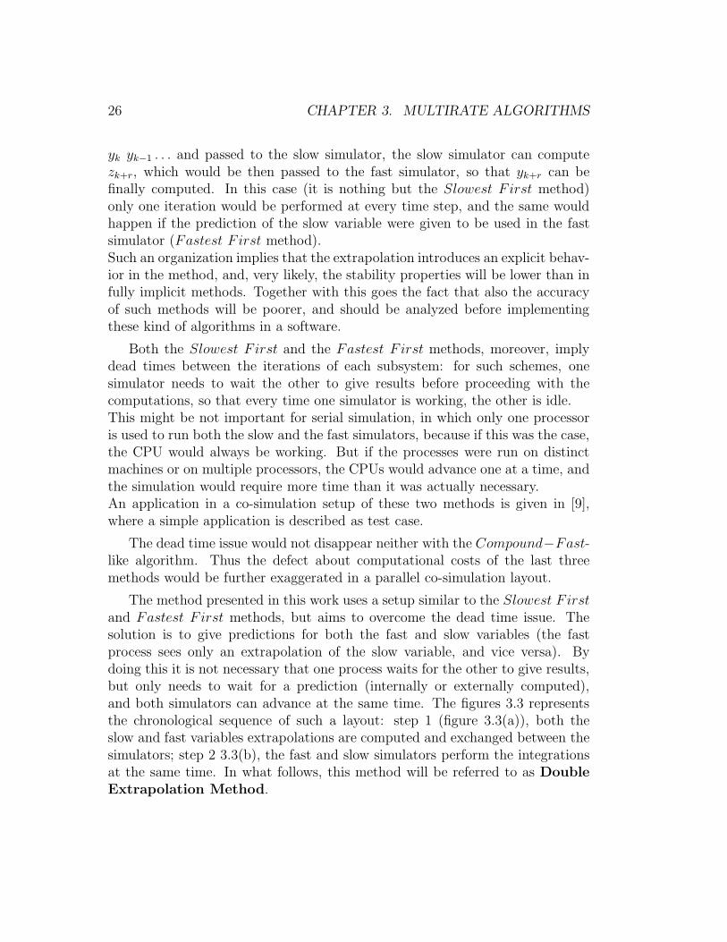
yk yk−1 . . . and passed to the slow simulator, the slow simulator can computezk+r, which would be then passed to the fast simulator, so that yk+r can befinally computed. In this case (it is nothing but the Slowest F irst method)only one iteration would be performed at every time step, and the same wouldhappen if the prediction of the slow variable were given to be used in the fastsimulator (Fastest F irst method).Such an organization implies that the extrapolation introduces an explicit behav-ior in the method, and, very likely, the stability properties will be lower than infully implicit methods. Together with this goes the fact that also the accuracyof such methods will be poorer, and should be analyzed before implementingthese kind of algorithms in a software.
Both the Slowest F irst and the Fastest F irst methods, moreover, implydead times between the iterations of each subsystem: for such schemes, onesimulator needs to wait the other to give results before proceeding with thecomputations, so that every time one simulator is working, the other is idle.This might be not important for serial simulation, in which only one processoris used to run both the slow and the fast simulators, because if this was the case,the CPU would always be working. But if the processes were run on distinctmachines or on multiple processors, the CPUs would advance one at a time, andthe simulation would require more time than it was actually necessary.An application in a co-simulation setup of these two methods is given in [9],where a simple application is described as test case.
The dead time issue would not disappear neither with the Compound−Fast-like algorithm. Thus the defect about computational costs of the last threemethods would be further exaggerated in a parallel co-simulation layout.
The method presented in this work uses a setup similar to the Slowest F irst
and Fastest F irst methods, but aims to overcome the dead time issue. Thesolution is to give predictions for both the fast and slow variables (the fastprocess sees only an extrapolation of the slow variable, and vice versa). Bydoing this it is not necessary that one process waits for the other to give results,but only needs to wait for a prediction (internally or externally computed),and both simulators can advance at the same time. The figures 3.3 representsthe chronological sequence of such a layout: step 1 (figure 3.3(a)), both theslow and fast variables extrapolations are computed and exchanged between thesimulators; step 2 3.3(b), the fast and slow simulators perform the integrationsat the same time. In what follows, this method will be referred to as DoubleExtrapolation Method.

3.3. NEW ALGORITHM DEFINITION 27
k-r .. ... .. k-3 k-2 k-1 k k+1 k+2 k+r
Fast Variable
ystored values
yextrap
k-r k k+r
Slow Variable
zstored values
zextrap
(a) Step 1
k-r .. ... .. k-3 k-2 k-1 k k+1 k+2 k+r
Fast Variable
ynew value
k-r k k+r
Slow Variable
znew value
(b) Step 2
Figure 3.3: Double Extrapolation chronological sequence.
3.3 New Algorithm Definition
As already stated, in the case the two subsystems are integrated by differentprocesses, it is convenient to carry out the integration using predicted values ofthe external variable, and then advance by an implicit scheme.
The method described in this work makes use of a linear multistep implicitmethod. In contrast to a single-rate method (defined in (3.1.2)), the solution of(3.1.1) in a multirate layout is given by (3.3.1).
yi+1 =
p−1∑
j=0
(ajyi−j + hbj fi−j) + hbpfi+1 (3.3.1a)
z(i+1)r =
p−1∑
j=0
(ajz(i−j)r +Hbj g(i−j)r) +Hbpgi+1 (3.3.1b)
where fi = f(ti, yi, zi), gi = g(ti, yi, zi) and y and z are approximation to y
and z respectively. Both methods have order p. Note that both methods havebp 6= 0, i.e. both are implicit. In addition, the two subsystems are integratedwith different timesteps (h and H), thus giving a multirate scheme. The ratior = h
His called the multirate ratio.
In general, different strategies could be adopted to approximate y and z, andeven if the same Multistep Method is adopted as internal solver, the approxima-tion strategies may generate even extremely different performances, especiallyin terms of stability.

28 CHAPTER 3. MULTIRATE ALGORITHMS
As already stated, the method proposed in this work makes use of extrapola-tions (based on explicit Linear Multistep Methods) to predict both the fast andthe slow variable. Moreover, a 2 steps BDF will be selected as internal solverfor both processes.
3.3.1 Extrapolation method
Extrapolation is given based on state variable and state derivative old values,as for the explicit Multistep Methods.
Considerations about accuracy, efficiency, memory usage and computationalcosts bring to the conclusion that the best choice is to use a maximum of 2 stepsfor predictions, thus relating the computation on already stored old variablesvalues (being the integrators built on a BDF 2 steps).
The slow integrator uses a constant (zero-order) extrapolation of the fastvariable, because it is not possible to determine a higher order formula showinggood behavior in every situations, being the extrapolation step always too largecompared to the frequency of the signal.
For use in the fast integrator, the slow variable can be predicted by a higherorder scheme (linear or quadratic), using the values of the most recent stepsavailable. Increasing the order to a cubic extrapolation will decrease the stabilityperformance if only 2 steps are used, and will increase the memory requirementsif more than 2 steps are required. Thus, no cubic extrapolation is considered inthis work.Even if both linear and quadratic extrapolations will be implemented in thesoftware, the rest of the thesis will focus only on quadratic extrapolation, sincethis algorithm shows better performances.
3.4 The Single-rate Layout
The case in which the two subsystems are integrated with the same time step isof course a special case of the general layout described in the previous sections.
This case is referred to as single-rate (multirate ratio r = 1). If this were thecase, the distinction between fast and slow variables does not exist any more,and the considerations in section 3.3.1 are no longer valid: in a sinlge-rate layoutthe extrapolation of both variables can be carried out by the same higher ordermethod.
3.5. STABILITY ANALYSIS 29
3.5 Stability Analysis
Traditionally, Multistep Methods applied to test problems generate differenceequations [11]. Once the difference equation is determined, the stability con-dition is translated in the roots condition: the method is said to be absolutelystable if and only if all the roots of the characteristic polynomial have an absolutevalue less than or equal to one.
In this work, it is not possible to select a single differential equation as a testproblem, since the aim is to analyze the interaction between different systems.A system of ODEs is instead to be used, for which the application of a MultistepMethod gives a system of difference equations. This system can be writtenby means of a matrix, called the Compound Matrix. The stability analysis isthus carried out through the study of the compound matrix, as in [7], [10]. Inparticular, the roots condition becomes the spectral radius condition, and themethod is said to be absolutely stable if and only if the spectral radius of thecompound matrix is less than or equal to one.
3.5.1 Compound Matrix
Here below a method is given to build the compound matrix for the generalcases of Multistep Linear Multirate Methods, where the coupled terms are ap-proximated either in terms of interpolation or extrapolation, considering bothimplicit and explicit schemes. After this, such a method will be applied to theparticular case of interest. The reason why no restrictions are imposed at thislevel is to build an instrument giving the possibility to evaluate, also in thefuture, possible modifications and improvements.
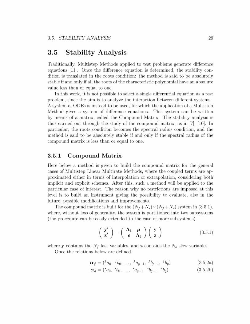
The compound matrix is built for the (Nf+Ns)×(Nf+Ns) system in (3.5.1),where, without loss of generality, the system is partitioned into two subsystems(the procedure can be easily extended to the case of more subsystems).
(
y′
z′
)
=
(
Λ1 µ
ε Λ2
)(
yz
)
(3.5.1)
where y contains the Nf fast variables, and z contains the Ns slow variables.Once the relations below are defined
αf = (fa0,fb0, . . . ,
fap−1,fbp−1,
fbp) (3.5.2a)
αs = (sa0,sb0, . . . ,
saq−1,sbq−1,
sbq) (3.5.2b)

30 CHAPTER 3. MULTIRATE ALGORITHMS
Af = A(αf) =
fa0Ifb0I · · · · · · fap−1I
fbp−1I0 0 · · · · · · 0 0
I ......
(3.5.3a)
As = A(αs) =
sa0Isb0I · · · · · · saq−1I
sbq−1I0 0 · · · · · · 0 0
I ......
(3.5.3b)
βf = β(αf) =(fbpI, I, 0, . . . , 0)T (3.5.4a)
βs = β(αs) =(sbqI, I, 0, . . . , 0)T (3.5.4b)
Yi = (yTi , f
Ti , . . . ,y
Ti−p+1, f
Ti−p+1)
T (3.5.5a)
Znk = (zTnk, gTnk, . . . , z
T(n−q+1)k, g
T(n−q+1)k)
T (3.5.5b)
the multistep method (3.3.1) applied to (3.5.1) gives the following relations
Yi+1 = AfYi + hβf fi+1 (3.5.6a)
Z(n+1)k = AsZnk +Hβsg(n+1)k (3.5.6b)
where i = nk, . . . , (n+ 1)k, and
fi+1 = Λ1yi+1 + µzi+1 (3.5.7a)
g(n+1)k = Λ2z(n+1)k + εy(n+1)k (3.5.7b)
A general way to define approximated values used in the simulation, consid-ering both extrapolation-based and implicit methods, is the following.
y(n+1)k = φfY(n+1)k (3.5.8)
zi+1 = φjZ(n+1)k (3.5.9)
with j = i− nk + 1. Details about φf and φj will be given in (3.5.13)

3.5. STABILITY ANALYSIS 31
Defining the rectangular matrices
E11 = (hΛ1, 0, . . . , 0)
E22 = (HΛ2, 0, . . . , 0)
E12 = (hµ, 0, . . . , 0)
E21 = (Hε, 0, . . . , 0)
leads to
Yi+1 = AfYi +B11Yi+1 +B12φjZ(n+1)k (3.5.10a)
Z(n+1)k = AsZnk +B22Z(n+1)k +B21φfY(n+1)k (3.5.10b)
where:
B11 = βfE11
B12 = βfE12
B21 = βsE21
B22 = βsE22
Defining the new matrices
Λf = (I+B11)−1Af
Λs = (I+B22)−1As
Γf i = (I+B11)−1B12Φj
Γs = (I+B22)−1B21Φf
the system (3.5.10) can be written using a more compact notation:
Yi+1 = ΛfYi + Γf iZ(n+1)k (3.5.11a)
Z(n+1)k = ΛsZnk + ΓsY(n+1)k (3.5.11b)
and the compound step is finally given by
Y(n+1)k = ΛfkYnk +
k−1∑
i=0
Λf(k−1−i)Γf iZnk (3.5.12a)
Z(n+1)k = ΛsZnk + ΓsYnk (3.5.12b)

32 CHAPTER 3. MULTIRATE ALGORITHMS
Extrapolation algorithm
The matrices φf and φi define the extrapolation algorithm. Changing the ex-trapolation technique will carry to different methods: fully implicit, SlowestFirst, Fastest First, and so on.
Once the algorithm is chosen, building such matrices is straightforward. Theexample leading to the new method presented in this work is given here below.
φf = (0, 0, I, 0, . . . , 0) (3.5.13a)
φi = (0, 0,i v0I,i d0I, . . . ,
i vq−1I,i dq−1I) (3.5.13b)
where the coefficients ivkidk define the extrapolation method for the slow vari-
able.
In the same way, it is easy to show how the traditional algorithm can bedefined in this context. For the Slowest First method:
φf = (0, 0, I, 0, . . . , 0) (3.5.14a)
φi = (im0I,i n0I,
i m−1I,i n−1I, 0, . . . , 0) (3.5.14b)
where the coefficients imkink define the interpolation method for the slow vari-
able.
For the Fastest First method:
φf = (I, 0, . . . , 0) (3.5.15a)
φi = (0, 0,i v0I,i d0I, . . . ,
i vq−1I,i dq−1I) (3.5.15b)
By such an approach, changing the coefficients in (3.5.2), (3.5.4) and (3.5.13),(3.5.14) or (3.5.15), the stability properties of many linear Multistep Multirateschemes, applied to a general linear ODE system, can be determined.
3.5.2 Test Equation and Results
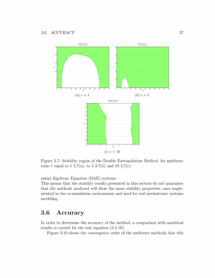
Results in terms of stability performances are given comparing the stabilityregion of the traditional BDF scheme with some multirate methods. In particu-lar, results are presented for the Double Extrapolation Method, for a comparisonwith the most similar traditional multirate algorithm, the Slowest First and theFastest First.

3.5. STABILITY ANALYSIS 33
To this aim, the linearized two-dimensional ODE system (3.5.16) is used.
(
y′
z′
)
=
(
λ µ
ε αλ
)(
y
z
)
(3.5.16)
where λ = p+ jω is a complex number, j is the imaginary unit and α < 1 is thefrequency ratio.
Now, consider the systems in which p = 0. If the stability of the algorithmhaves to be determined, it is necessary to select linear systems with simplestability (without positive nor negative damping). This means that the diagonalterms in (3.5.16) must be imaginary, and the real part of the eigenvalues mustbe set to zero. For the system (3.5.16) with λ pure imaginary, it is easy todemonstrate that this condition leads to
µε
(ω1−ω2
2)2
< 1 (3.5.17)
The ratio in (3.5.17) will be used also in the general case in which p 6= 0, togive the measure of the coupling of the subsystems, defined in (3.5.18):
β =µε
(ω1−ω2
2)2
(3.5.18)
β is thus the measure of the coupling, and imposing β < 1 gives simply stablesystems for λ pure imaginary.
The stability of the Multirate Methods has been analyzed since the beginningof the 1980s, exploiting different ways.
A stability analysis can be found in [10], where, however, damped systemsare selected to define stability regions of the methods. Thus, the regions definedin that work are wider than actual regions.
Also in [7] a stability analysis is presented. In that case, for a general caseof a Multirate Linear Multistep Method, the spectral radius of the compoundmatrix is studied indirectly using a 2x2 matrix M for which the spectral radiusρ(M) is demonstrated to be higher than the actual compound matrix spectralradius ρ(M), thus having ρ(M) < 1 necessarily leads to ρ(M) < 1. Thus, inthis case the region determined is narrower than the actual one.
In this work, the stability region bounds are not given in closed form. Foreach case considered, only the graphical representation of the region is presented.As traditionally done for the numerical integration methods, the stability regions

34 CHAPTER 3. MULTIRATE ALGORITHMS
are determined on the complex plane. For a single equation such as y′ = λy,the points of the complex plane correspond to hλ, with h being the dimensionof the time step and λ a complex number. For the system in (3.5.16), the sameconvention is adopted, and the points of the complex plane in the figures shownin this work always correspond to hλ, with h being the time step size. In all thefigures, the green area represents the stability region.
The results for the test case with α = 0.1 and β = 0.1 are shown in figuresfrom 3.4 to 3.7. In figure 3.4 the stability region of the traditional BDF method isdrawn (it is given only for comparison), while figures 3.5 and 3.6 show the SlowestFirst and the Fastest First case respectively, and figures 3.7 finally represent thestability results for the Double Extrapolation Method.
Re
Im
Traditional BDF methodα = 0.1 β = 0.1
−5 0 5 10 15 20 25 30 35 40 45 50
5
10
15
20
25
Figure 3.4: Stability region of the BDF Method
The Fastest First and the Double Extrapolation methods loose the A-stabilityfaster than the Slowest First (figures 3.7(c) and 3.6(c)).
The Double Extrapolation Method has worse stability properties comparedto the other two methods, for higher multirate ratios. This is obviously dueto the fact that the traditional SF and FF methods use only extrapolated val-ues for one subsystem, while for the other the actual solution is used. In theDouble Extrapolation Method, instead, two extrapolations are used, leading toa stronger explicit character of the method, which make the formula loose thestability properties a little faster. This kind of layout was the one chosen indefining the new method to avoid dead times (as already mentioned in section3.2), and this behavior of stability properties was expected.

3.5. STABILITY ANALYSIS 35
Re
Im
Multirate Ratio = 1α = 0.1 β = 0.1
−5 0 5 10 15 20 25 30 35 40 45 50
5
10
15
20
25
(a) r = 1
Re
Im
Multirate Ratio = 5α = 0.1 β = 0.1
−2 0 2 4 6 8 10 12 14 16 18 20
2
4
6
8
10
12
14
16
18
20
(b) r = 5
Re
Im
Multirate Ratio = 10α = 0.1 β = 0.1
−1 0 1 2 3 4 5
0.5
1
1.5
2
2.5
3
(c) r = 10
Figure 3.5: Stability region of the Slowest First Method, for multirate ratio r
equal to 1 3.5(a), to 5 3.5(b) and 10 3.5(c)
It must be noted that the Double Extrapolation Method does not loose thestability on the imaginary axis, for multirate ratio equal to 1 (3.7(a)) and to5 (3.7(b)). For r = 10, the stability condition is slightly lost, and the methodgives acceptable results only for systems that are at least weakly damped.
It is important to understand how the stability performances change byvarying the parameters α and β. Figures 3.8 show the behavior of the stabilityregion for the Double Extrapolation method when the parameter α changes from0.001 (figure 3.8(d)) to 0.01 (figure 3.8(a)), and β = 0.05 Again, it is of interestto observe the stability properties on the imaginary axis: for α = 0.1 and 0.05(figures 3.8(a) 3.8(b)), the stability is unconditioned, and there is no restrictionin selecting the time step for undamped systems. Figures 3.8(c) 3.8(d), instead,

36 CHAPTER 3. MULTIRATE ALGORITHMS
Re
ImMultirate Ratio = 1α = 0.1 β = 0.1
−10 0 10 20 30 40 50
5
10
15
20
25
30
(a) r = 1
Re
Im
Multirate Ratio = 5α = 0.1 β = 0.1
−2 0 2 4 6 8 10
0.5
1
1.5
2
2.5
3
3.5
4
4.5
5
5.5
6
(b) r = 5
Re
Im
Multirate Ratio = 10α = 0.1 β = 0.1
−2 0 2 4 6 8 10
0.5
1
1.5
2
2.5
3
3.5
4
4.5
5
5.5
6
(c) r = 10
Figure 3.6: Stability region of the Fastest First Method, for multirate ratio r
equal to 1 3.6(a), to 5 3.6(b) and 10 3.6(c)
show two conditionally stable methods, where stability is reached only for afinite interval of time step values.
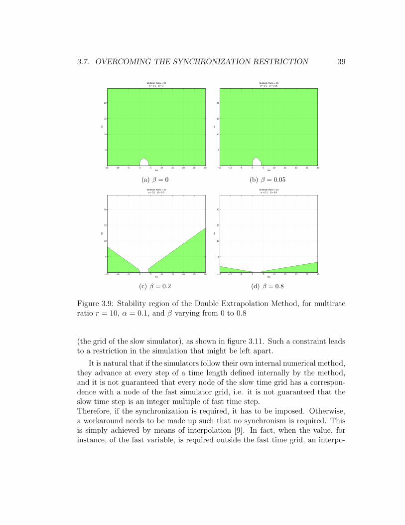
In figures 3.8 the change in the stability region is shown for β varying from0 (meaning no coupling between the susbsystems, figure 3.9(a)) to 0.8 (figure3.9(d)).
3.5.3 Validity of Stability Results
To analyze the stability performances of the methods, a linear ODE system hasbeen selected.The systems the multibody simulators deal with, however, are nonlinear Differ-
3.6. ACCURACY 37
Re
Im
Multirate Ratio = 1α = 0.1 β = 0.1
−5 0 5 10 15 20 25 30 35 40 45 50
5
10
15
20
25
(a) r = 1
Re
Im
Multirate Ratio = 5α = 0.1 β = 0.1
−5 0 5 10 15 20 25 30 35 40 45 50
5
10
15
20
25
(b) r = 5
Re
Im
Multirate Ratio = 10α = 0.1 β = 0.1
−3 −2 −1 0 1 2 3 4 5
0.5
1
1.5
2
2.5
3
3.5
4
4.5
5
(c) r = 10
Figure 3.7: Stability region of the Double Extrapolation Method, for multirateratio r equal to 1 3.7(a), to 5 3.7(b) and 10 3.7(c)
ential Algebraic Equation (DAE) systems.This means that the stability results presented in this section do not guaranteethat the methods analyzed will show the same stability properties, once imple-mented in the co-simulation environment and used for real mechatronic systemsmodeling.
3.6 Accuracy
In order to determine the accuracy of the method, a comparison with analiticalresults is carried for the test equation (3.5.16).
Figure 3.10 shows the convergence order of the multirate methods that this

38 CHAPTER 3. MULTIRATE ALGORITHMS
Re
ImMultirate Ratio = 10α = 0.1 β = 0.05
−15 −10 −5 0 5 10 15 20 25 30
5
10
15
20
(a) α = 0.1
Re
Im
Multirate Ratio = 10α = 0.05 β = 0.05
−15 −10 −5 0 5 10 15 20 25 30
5
10
15
20
(b) α = 0.05
Re
Im
Multirate Ratio = 10α = 0.01 β = 0.05
−15 −10 −5 0 5 10 15 20 25 30
5
10
15
20
(c) α = 0.01
Re
Im
Multirate Ratio = 10α = 0.001 β = 0.05
−15 −10 −5 0 5 10 15 20 25 30
5
10
15
20
(d) α = 0.001
Figure 3.8: Stability region of the Double Extrapolation Method, for multirateratio r = 10, β = 0.05, and α varying from 0.001 to 0.01
thesis deals with. Error is expressed in Linf norm. It is easy to note that forlarger values of the coupling coefficient β the order of convergence lowers from2 to about 1.
3.7 Overcoming the Synchronization Restric-
tion
An additional improvement regards the synchronization between the distinctprocesses. In what it has been discussed so far, it is implied that the processesexchange data at every macro step, at the time instants of the coarse time mesh
3.7. OVERCOMING THE SYNCHRONIZATION RESTRICTION 39
Re
Im
Multirate Ratio = 10α = 0.1 β = 0
−15 −10 −5 0 5 10 15 20 25 30
5
10
15
20
(a) β = 0
Re
Im
Multirate Ratio = 10α = 0.1 β = 0.05
−15 −10 −5 0 5 10 15 20 25 30
5
10
15
20
(b) β = 0.05
Re
Im
Multirate Ratio = 10α = 0.1 β = 0.2
−15 −10 −5 0 5 10 15 20 25 30
5
10
15
20
(c) β = 0.2
Re
Im
Multirate Ratio = 10α = 0.1 β = 0.8
−15 −10 −5 0 5 10 15 20 25 30
5
10
15
20
(d) β = 0.8
Figure 3.9: Stability region of the Double Extrapolation Method, for multirateratio r = 10, α = 0.1, and β varying from 0 to 0.8
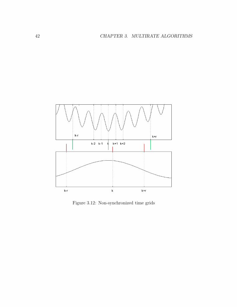
(the grid of the slow simulator), as shown in figure 3.11. Such a constraint leadsto a restriction in the simulation that might be left apart.
It is natural that if the simulators follow their own internal numerical method,they advance at every step of a time length defined internally by the method,and it is not guaranteed that every node of the slow time grid has a correspon-dence with a node of the fast simulator grid, i.e. it is not guaranteed that theslow time step is an integer multiple of fast time step.Therefore, if the synchronization is required, it has to be imposed. Otherwise,a workaround needs to be made up such that no synchronism is required. Thisis simply achieved by means of interpolation [9]. In fact, when the value, forinstance, of the fast variable, is required outside the fast time grid, an interpo-

40 CHAPTER 3. MULTIRATE ALGORITHMS
1e-07
1e-06
1e-05
0.0001
0.001
0.01
0.1
1
0.001 0.01 0.1
err
or
Timestep
Double ExtrapSlowest FirstFastest First
O(h)O(h
2)
(a) β = 0
1e-07
1e-06
1e-05
0.0001
0.001
0.01
0.1
1
0.001 0.01 0.1
err
or
Timestep
Double ExtrapSlowest FirstFastest First
O(h)O(h
2)
(b) β = 0.01
1e-07
1e-06
1e-05
0.0001
0.001
0.01
0.1
1
0.001 0.01 0.1
err
or
Timestep
Double ExtrapSlowest FirstFastest First
O(h)O(h
2)
(c) β = 0.05
1e-07
1e-06
1e-05
0.0001
0.001
0.01
0.1
1
0.001 0.01 0.1
err
or
Timestep
Double ExtrapSlowest FirstFastest First
O(h)O(h
2)
(d) β = 0.1
Figure 3.10: Convergence plot for the Double Extrapolation, Slowest First andFastest First methods, for α = 0.1 and different values of β.
lation is executed using the two or more nearest grid nodes, as shown in figure3.12.
It must be noted that with the Double Extrapolation scheme coupled witha 2 steps BDF , (which is the method proposed in this work, this workaround isautomatically implemented in the method itself, because each subsystem onlysees an extrapolated value of the external variable, as can be easily understoodby looking at (3.5.2), and considering that, for the BDF methods, fb0, . . . ,
fbp−1
and sb0, . . . ,sbq−1 are all zeros.
Thus, for both the subsystems (both use BDF ), when the extrapolation algo-rithm is called, this is automatically set to calculate the values of the externalvariable at the nodes of the internal time grid.

3.7. OVERCOMING THE SYNCHRONIZATION RESTRICTION 41
Figure 3.11: Synchronized time grids setup
42 CHAPTER 3. MULTIRATE ALGORITHMS
Figure 3.12: Non-synchronized time grids

Chapter 4
Software Environment Design
The software environment is constructed by basically choosing a Multibody anda block scheme simulators, and the way the two tools will communicate. Asthe general intent of this work is to begin a longer term developing, directlyinvolving as many users as possible, free softwares will be selected. It is likelythat, during the developing of a layout such as the one proposed in this work,some extensions will have to be added to the software tools initially selected.This is another causal factor addressing the choice on free softwares, as thiscategory is intrinsically proposed to the users as a base to construct new tools,rather than just out of the box instruments.
4.1 Software Tools Selection
4.1.1 Multibody Simulator
The multibody simulator selected is MBDyn [20], a free software developedat Dipartimento di Ingegneria Aerospaziale of Politecnico di Milano (DIAPM),Italy.
MBDyn is already predisposed for external communication, both in localand network layout. The functions implemented use Internet sockets and Unixdomain sockets, which basically drive endpoints of bidirectional communicationon the kernel ports. The Stream drive is the function making the communicationavailable (see MBDyn input manual for details [17]).
The analyses this software performs are based on an original formulation forthe direct time integration of Initial Value Problems (IVP), which is written as
43
44 CHAPTER 4. SOFTWARE ENVIRONMENT DESIGN
a system of first-order Differential-Algebraic Equations (DAE), using implicit(nearly) L-stable integration algorithms [12].
Unconstrained Dynamics
The equations of motion (EOMs) of a general mechanical system are usuallyderived by the Newton-Euler approach. For a system of unconstrained bodies,EOMs are described by
M(q)q = l(q, q, t) (4.1.1)
If nb is the number of nodes forming the system, n = 6nb is the dimension ofthe system (the number of equations and degrees of freedom).q ∈ R
n contains the kinematic variables of the nodes (or the generalized coor-dinates), and M(q) is the mass matrix, which may depend on q.l(q, q, t) is the function describing the external forces acting on nodes, and mayinclude structural deformability contributions.Written in the form of a first order system, equation (4.1.1) becomes
M(q)q = p (4.1.2a)
p = l(q, q,p, t) (4.1.2b)
where p ∈ Rn is the momenta and momentum moments vector.
Constrained Dynamics
There exist two types of constraints, holonomic and non-holonomic. Both aremodeled by adding explicit algebraic relations
0 = Φ(q, t) (4.1.3)
in the case of holonomic constraints, while for non-holonomic constraints
0 = Ψ(q, q, t) (4.1.4)
4.1. SOFTWARE TOOLS SELECTION 45
By using Lagrange’s multipliers formalism, system (4.1.2b) becomes
M(q)q = p (4.1.5a)
p+ΦT/qλ+ΨT
/qµ = l(q, q,p, t) (4.1.5b)
Φ(q, t) = 0 (4.1.5c)
Ψ(q, q, t) = 0 (4.1.5d)
where λ and µ are the Lagrange’s multipliers.
Numerical Integration
The Differential Algebraic Equation system (4.1.5d) has the general form
h(x,x, t) = 0 (4.1.6)
where x = (q,p, λ, µ)T.
The numerical solution at time tk+1 by means of the general multistepmethod (3.1.2) is obtained by solving (4.1.6) for xk+1 with
xk+1 =
p−1∑
j=0
(ajxk−j + hbjxk−j) + hbpxk+1 (4.1.7)
Using a Newton-Raphson scheme, the solution is given by
h/xδxk+1 + h/xδxk+1 = −h (4.1.8)
Inserting (4.1.7) in (4.1.8) yields
(h/x + hbph/x)δxk+1 = −h (4.1.9)
because
δxk+1 = hbpδxk+1 (4.1.10)
For each time step (that is, for each instant tk of the time grid), iterationsare performed to solve (4.1.9), until convergence is reached.
46 CHAPTER 4. SOFTWARE ENVIRONMENT DESIGN
Multirate Numerical Integration
If the system is divided into two subsystems, equation (4.1.6) becomes
f(y,y, z, t) = 0 (4.1.11)
g(z, z,y, t) = 0 (4.1.12)
and if a generic multirate multistep scheme is used, as the one in (3.3.1), timederivatives for the new time step are computed based on interpolations or ex-trapolations of old values. Equation (4.1.7) is transformed into
yk+1 =
p−1∑
j=0
(ajyk−j + hbjyk−j) + hbp ˙yk+1 (4.1.13a)
z(k+1)r =
p−1∑
j=0
(ajz(k−j)r +Hbj z(k−j)r) +Hbp ˙z(k+1)r (4.1.13b)
As described in section 3.3, ˙y and ˙z are approximations of y and z, respectively,h is the small time step and H is the large time step.If extrapolation from old values is used to compute approximations
˙yk+1 = α(yk+1, zk, . . . , z(k−q)r) (4.1.14a)
˙z(k+1)r = β(z(k+1)r,ykr, . . . ,ykr−o) (4.1.14b)
where q and o are the order of slow variable and fast variable extrapolations,respectively.
Equations (4.1.8) and (4.1.9) formally do not change, except for the fact thatapproximated values are used for time derivatives.
If both equations in (4.1.14) are followed, the Double Extrapolation Methodpresented in section 3.2 is obtained.
Depending on the approximation technique, several multirate methods canbe carried out following this procedure:
• If the fast variable derivative is computed by (4.1.14a) and the slow vari-able derivative is the actual solution (thus ˙z(k+1)r = z(k+1)r), the FastestFirst Method is derived.
• If the slow variable derivative is computed by (4.1.14b) and the fast vari-able derivative is computed by interpolation, the Slowest First Method is
4.2. INTER-PROCESS COMMUNICATION 47
derived.
• If the slow variable derivative is given in terms of actual value and the fastvariable derivative is computed by interpolation, a fully implicit methodis constructed, such as the Compound-Fast, the General Compound-Fastand the Mixed Compound-Fast methods.
4.1.2 Block Scheme Simulator
This kind of simulators have been developed for many years by different groups:examples are Simulink [21] by Mathworks, SystemBuild [22] by National Instru-ments and the Scicos [23] based ScicosLab [24] by INRIA and Xcos [25] by theScilab Consortium.
Considering the efficiency and the versatility, Simulink is probably the bestsimulator available. On the other side, if the user freedom (see section 1.2) re-lated to the software is the argument driving the comparison, ScicosLab becomesthe best candidate. All the indicated simulators, though, are widely recognizedby the industry and the academic world to be valid instruments.
The choice has been directed to ScicosLab. Since the Scicos based simu-lators have very similar properties and function calls, the developed MBDyninterface has been tested both with Scilab (Scicos until the 5.1.x versions andXcos since 5.2.x) and ScicosLab, and both will be proposed to the MBDyn andScicos/ScicosLab users. Minor differences distinguish the two versions.
Even though no particular communication functions are implemented in Sci-cos (other that text and audio file interactions) to talk to external processes, itis possible to define new blocks by compiling and linking user defined functionswritten in C, Fortran or Scilab language. This possibility has been exploited toconstruct socket based communications (both in local and network setup).
4.2 Inter-process Communication
The inter-process communication is constructed based on TCP/IP Internet sock-ets (with the local communication being a special subcase of the network-baseddata exchange). This kind of data transmission is very efficient (way morethan, for example, employing text file read/write functions), and it is natu-rally directed to multiple machines layout, which, in many cases, can sensitivelydecrease the time-to-solution.

48 CHAPTER 4. SOFTWARE ENVIRONMENT DESIGN
In the layout used for the cases presented here, the multibody software MB-Dyn and the block diagram simulator Scicos communicate through blocking
sockets (the process reading informations waits until all the expected data areavailable). In this way, the communication process acts also as synchronizer.
4.3 A Simple Test
An inverse pendulum has been used as a test bench of the software tool designed.The problem consists in controlling the angular position of the pendulum bymeans of a PD controller. This case is used to show the way the simulatoroperates. A single-rate layout is used.
Figure 4.1: Inverse pendulum multibody model: the force F is used to controlthe angular position of the pendulum
In this case, MBDyn creates a server socket on a kernel port, and waits untilScicos creates the client socket on the same port. After the connection succeeds,the simulation starts: at each time step, MBDyn solves the nonlinear dynamicsof the pendulum, and is asked to output the angular position and the angularvelocity of the pendulum, which are written as doubles on the kernel port. Scicosreads the data on the port, computes the control force, and write it on the sameport as before. At the next step, MBDyn computes the motion of the pendulumreading the input force from the socket, and so on until the simulation ends.
Angular position and input force resulting form the co-simulation are shownin figures 4.3

4.4. FUTURE ENHANCEMENT 49
Pendulum
Input force
0.1
Position
200
10
−
+
READMBDyn
WRITEMBDyn
Figure 4.2: PD controller: position and angular velocity are used to computethe control force
0 50 100 150 2000.00
0.02
0.04
0.06
0.08
0.10
0.12
0.14
0.16
0.18
0.20
Angular position
t
The
ta [r
ad]
(a) Angular position vs time
0 50 100 150 200−30
−25
−20
−15
−10
−5
0
5
10
15
20
Input force
t
For
ce [N
]
(b) Input force vs time
Figure 4.3: Inverse pendulum results
4.4 Future Enhancement
A possible advantage might be introduced with a Predictor-Corrector setup.For such a layout, the method exposed here (Double Extrapolation) could beused for both the prediction and the correction (with the difference that in thecorrection iteration, the predicted values are used instead of the extrapolations).Improvement either in terms of accuracy and stability should be expected forthis extension.
Another possibility is to integrate the system (3.1.1) by an implicit step,implementing different methods, such as those described in sections 3.2.3, 3.2.4and 3.2.5. This kind of implementation, as already stated in section 3.2, couldresult in an inefficient setup. However, enhanced stability and accuracy proper-

50 CHAPTER 4. SOFTWARE ENVIRONMENT DESIGN
ties should be expected. It is possible that such a layout would be useful onlyfor batch simulation, while real-time simulations would be carried out in otherways.
Chapter 5
Wind Energy Application
The aim of this chapter is to illustrate the feasibility of the working environmentdeveloped.
In order to test the performances of the working environment, a model of areal plant has been built, in which the coupling between active control, dynamics,and structural dynamics has a great relevance.
The plant considered between all the possible applications to test the co-simulation setup is a controlled wind turbine. Specifically, the CART (ControlsAdvanced Research Turbine) has been selected.
Wind turbines are usually operated in different working regions (start-up,maximum power, constant power, shutdown, ...), and active controls are usedto maximize power production, maintain safe operation and limiting structural(static and fatigue) loads in all the working conditions [14].
The multidisciplinary environment is used to analyze the coupling betweenthe wind turbine dynamics and a simple baseline controller, managing the bladepitch and the electrical generator power production.
The CART being the object of this chapter, it will be briefly described inthe next section.
5.1 CART Description
The CART is a two-bladed, upwind, variable speed wind turbine, rated at 600KW. It is located at the National Wind Technology Center (NWTC) and wasinstalled as a test-bench to design new control schemes in wind power generation.The rotor has a diameter of 43.3 m and hub height is 36.6 m. The electrical
51

52 CHAPTER 5. WIND ENERGY APPLICATION
Figure 5.1: The Control Advanced Research Turbine at NWTC, Colorado
generator is rated at 1800 rpm, and connected to the Low Speed Shaft througha two-state gearbox with a ratio of 43.165. The turbine rotor is thus rated at41.7 rpm.
5.2 Multibody Model
The computational model of the turbine is the same used in [15], freely availablefor download at [16] (under the name cart0) thank to the author, Luca Cavagna.
Deformable beam elements are used to model the tower and the blades struc-tural behavior. Rigid elements model the nacelle, the low-speed shaft and theteetering hub, while the generator is idealized as a torque acting between thenacelle and the low-speed shaft. Aerodynamic elements are used to model theaerodynamical properties of the blades. Table 5.1 quickly describes the multi-body model properties.
A graphical representation of the model is given in figure 5.2

5.3. CONTROLLER 53
Components Nodes Joints Bodies Beams Aero Forces DoFs
Tower 11 1 10 5 138Nacelle 1 2 1 17Shaft 1 1 1 17Generator 1Teeter 1 1 1 17Blade 2x 11 1 11 5 5 138Total 36 7 35 15 10 1 465
Table 5.1: Summary of CART multibody model
(a) General view (b) Rotor to tower connection detail
Figure 5.2: Graphical representation of the CART multibody model
5.3 Controller
A simple example for a variable-speed wind turbine controller is given in [14].Three working regions are defined:
Startup The rotor is starting, and no torque from the generator is applied
Region 2 The rotor is below rated speed. The generator torque is controlledto get the optimal Tip Speed Ratio (TSR), thus the maximum powergeneration
Transition Transition region to connect Region 2 and Region 3, to let theturbine reach the rated torque at rated speed
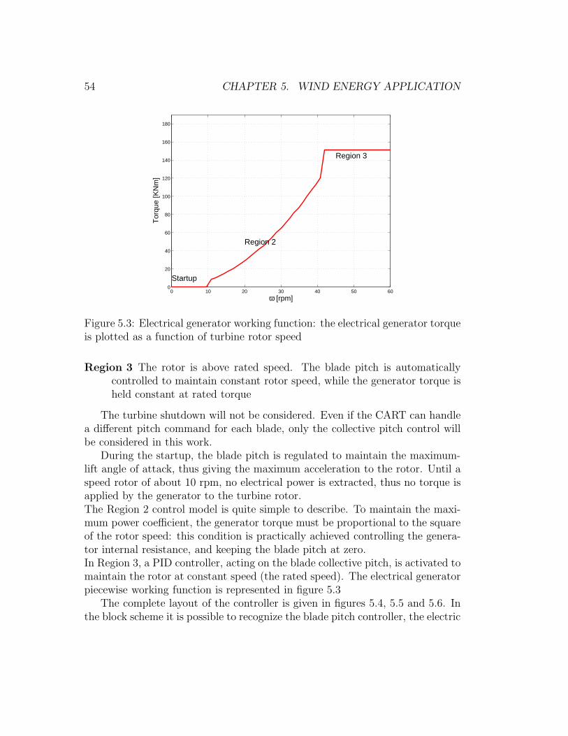
54 CHAPTER 5. WIND ENERGY APPLICATION
0 10 20 30 40 50 600
20
40
60
80
100
120
140
160
180
ω [rpm]
Tor
que
[KN
m]
Startup
Region 2
Region 3
Figure 5.3: Electrical generator working function: the electrical generator torqueis plotted as a function of turbine rotor speed
Region 3 The rotor is above rated speed. The blade pitch is automaticallycontrolled to maintain constant rotor speed, while the generator torque isheld constant at rated torque
The turbine shutdown will not be considered. Even if the CART can handlea different pitch command for each blade, only the collective pitch control willbe considered in this work.
During the startup, the blade pitch is regulated to maintain the maximum-lift angle of attack, thus giving the maximum acceleration to the rotor. Until aspeed rotor of about 10 rpm, no electrical power is extracted, thus no torque isapplied by the generator to the turbine rotor.The Region 2 control model is quite simple to describe. To maintain the maxi-mum power coefficient, the generator torque must be proportional to the squareof the rotor speed: this condition is practically achieved controlling the genera-tor internal resistance, and keeping the blade pitch at zero.In Region 3, a PID controller, acting on the blade collective pitch, is activated tomaintain the rotor at constant speed (the rated speed). The electrical generatorpiecewise working function is represented in figure 5.3
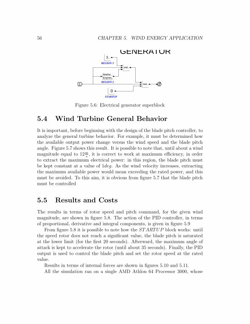
The complete layout of the controller is given in figures 5.4, 5.5 and 5.6. Inthe block scheme it is possible to recognize the blade pitch controller, the electric

5.3. CONTROLLER 55
CART
R..MB..
WR..MB..
den(s)num(s)
PITCH ENGINE
4..
RATED SPEED
SAT
57.3
PID
GENERATOR
output ..write to
CatVert
+−
den(s)num(s)
SPEED FILTER
60/(..
12
WIND SPEED
swi..
Expres..Mathe..
STARTUP
(2*..
Figure 5.4: Block Scheme of the controller implemented in Scicos
PID0.1
0.01
0.1
1/s
du/..
s
11
11
swi..
0
swi..
MA..
swi..
11
output ..write to
CatVert
2*%..
Figure 5.5: PID controller superblock
generator torque and the wind magnitude definitions.
The PITCH ENGINE block in figure 5.4 represents the blade pitch actu-ator transfer function, a second order Butterworth filter.
The STARTUP block acts in the first part of the simulation, to startup theturbine rotor. In this condition, the PID controller has to be bypassed becausethe blades need to point the airfoil nose into the wind. The PID controller, innormal conditions, basically increases the angle of attack (by incrementing theblade pitch) to increase the rotational speed. When the angle of attack is overthe stall limit (this occurs during the startup) this condition has to be inverted.The STARTUP block takes care of this inversion.
56 CHAPTER 5. WIND ENERGY APPLICATION
GENERATOR
1111
Expres..Mathe..
REGION 2
0STARTUP
3..
REGION 3
swi..
swi..
Figure 5.6: Electrical generator superblock
5.4 Wind Turbine General Behavior
It is important, before beginning with the design of the blade pitch controller, toanalyze the general turbine behavior. For example, it must be determined howthe available output power change versus the wind speed and the blade pitchangle. Figure 5.7 shows this result. It is possible to note that, until about a windmagnitude equal to 12m
s, it is correct to work at maximum efficiency, in order
to extract the maximum electrical power: in this region, the blade pitch mustbe kept constant at a value of 1deg. As the wind velocity increases, extractingthe maximum available power would mean exceeding the rated power, and thismust be avoided. To this aim, it is obvious from figure 5.7 that the blade pitchmust be controlled
5.5 Results and Costs
The results in terms of rotor speed and pitch command, for the given windmagnitude, are shown in figure 5.8. The action of the PID controller, in termsof proportional, derivative and integral components, is given in figure 5.9
From figure 5.8 it is possible to note how the STARTUP block works: untilthe speed rotor does not reach a significant value, the blade pitch is saturatedat the lower limit (for the first 20 seconds). Afterward, the maximum angle ofattack is kept to accelerate the rotor (until about 35 seconds). Finally, the PIDoutput is used to control the blade pitch and set the rotor speed at the ratedvalue.
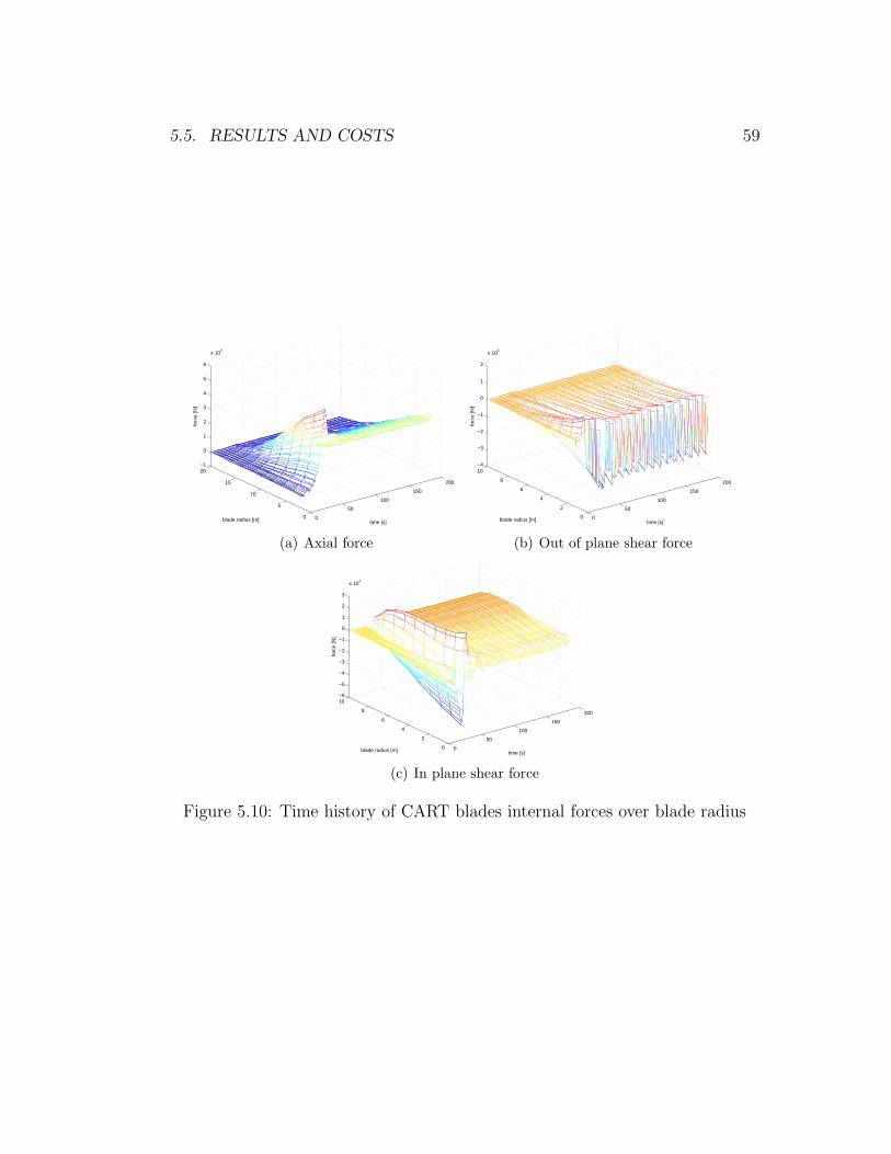
Results in terms of internal forces are shown in figures 5.10 and 5.11.All the simulation ran on a single AMD Athlon 64 Processor 3000, whose

5.5. RESULTS AND COSTS 57
0
200
400
600
800
1000
1200
4 6 8 10 12 14 16 18 20 22 0
200
400
600
800
1000
1200
Ava
ilab
le p
ower
[K
W]
Wind speed [m/s]
θ = 1θ = -5
θ = -10Rated Power
Figure 5.7: CART available power diagram: points represent data from simula-tions, continuous functions are the theoretical curves
-30
-20
-10
0
10
20
30
40
50
0 50 100 150 200
θ [d
eg],
Vin
f [m
/s],
Ω [
rpm
]
Time [s]
θVinf
Ω
Figure 5.8: Blade pitch, wind magnitude and rotor speed as functions of time

58 CHAPTER 5. WIND ENERGY APPLICATION
-20
-10
0
10
20
0 50 100 150 200
P [
deg]
, I [
deg]
, D [
deg]
Time [s]
PID controller output components
PI
D
Figure 5.9: PID controller action in terms of components
performances are given in table 5.2
CPU MHz 2002.5Cache Size 512 KB
Table 5.2: Processor performances
It is important to monitor the computational costs for the different simula-tion layouts. The working environment is made up of two different softwares:MBDyn and Scicos. The two components have big differences in terms of com-putational efficiency, with a great superiority for MBDyn. However, also themodel described in the softwares are definitely different: MBDyn analyzes thenonlinear dynamics of a complex mechanical system, while Scicos have to modela quite simple controller, with few nonlinearity.In conclusion, for the case presented here, the CPU time needed by MBDyn ismuch higher (20 times higher than the time needed by Scicos).
The overall CPU time required for the simulation in this case is 224330ms
(3min, 44s, 330ms). For MBdyn alone to simulate the same model, withoutexternal interaction to add the control loop, 185990ms (3min, 05s, 990ms) areneeded to complete the simulation.
5.5. RESULTS AND COSTS 59
0
50
100
150
200
0
5
10
15
20−1
0
1
2
3
4
5
6
x 105
time [s]blade radius [m]
forc
e [N
]
(a) Axial force
0
50
100
150
200
0
2
4
6
8
10−4
−3
−2
−1
0
1
2
x 104
time [s]blade radius [m]
forc
e [N
]
(b) Out of plane shear force
0
50
100
150
200
0
2
4
6
8
10−6
−5
−4
−3
−2
−1
0
1
2
3
x 104
time [s]blade radius [m]
forc
e [N
]
(c) In plane shear force
Figure 5.10: Time history of CART blades internal forces over blade radius

60 CHAPTER 5. WIND ENERGY APPLICATION
0
50
100
150
200
0
2
4
6
8
10−1
−0.5
0
0.5
1
1.5
x 104
time [s]blade radius [m]
mom
ent [
Nm
]
(a) Torsional moment
0
50
100
150
200
0
2
4
6
8
10−6
−4
−2
0
2
4
x 105
time [s]blade radius [m]
mom
ent [
Nm
]
(b) In plane bending moment
0
50
100
150
200
0
2
4
6
8
10−2
−1.5
−1
−0.5
0
0.5
1
1.5
x 105
time [s]blade radius [m]
mom
ent [
Nm
]
(c) Out of plane bending moment
Figure 5.11: Time history of CART blades internal moments over blade radius

5.6. MULTIRATE CPU TIME SAVING 61
5.6 Multirate CPU Time Saving
An interesting situation is represented by the multirate layout, in which MB-Dyn and Scicos simulate their own models integrating the equations at differentfrequencies.
It is common to have situations in which subsystems have different frequen-cies. In these cases, it happens that if the integration frequency is determinedbased on the fast subsystem characteristics, a high computational cost is reached,otherwise, if the slow subsystem is considered, the accuracy for the fast subsys-tem is lowered. To save CPU time and accuracy, the multirate layout may beemployed.
Considering the CART example, for instance, a detailed behavior of theelectrical generator, to analyze the oscillations in the output current, requiresa much smaller timestep, say 0.002s, while the previous simulation, to analyzethe turbine dynamics coupled with the pitch and torque controllers, has beencarried with a timestep of 0.01s.
The aim here is not to give a detailed analysis of the generator nor theturbine behavior, but rather to give an idea of what is the time saving due tousing the multirate layout to simulate the machine behavior.Therefore, the CPU time is determined relative to the simulation of the alreadypresented system, both in multirate layout and in singlerate (now with a refinedtimestep).The processor performances do not change, and the reference is again table 5.2.
The overall CPU time required for the singlerate simulation with a timestepof 0.002s is 934960ms (15min, 34s, 960ms).
It is obvious, by looking at the computational costs, that carrying such asimulation in a singlerate layout is not convenient at all, but one would prefer toextract the results from a simulation with a simpler model of the electrical gen-erator, and then build another model, in which the detailed generator behavioris described, giving the previous results as inputs.
An integrated way is, instead, to describe the detailed generator directlyin the general model, but then exploit the multirate layout. The simulationcarried with a timestep of 0.01s in MBDyn and 0.002s in Scicos, in this multiratecosimulation environment, costs 227810ms (3min, 47s, 810ms) of CPU.

62 CHAPTER 5. WIND ENERGY APPLICATION
5.7 Wind Turbine Modeling Objective
Wind turbines are usually driven by automatic controllers for two reasons: en-sure a smooth time evolution of loads and electrical power and reduce the poweroutput (as well as rotor velocity) at high wind speed.
The second aim is directed in both reducing the costs of the plant and in-creasing the safety of operations. This corresponds to the reason why a bladepitch controller has been applied to the CART.
The electrical generator torque control is achieved by simply defining a func-tional relation between the rotational speed and the generator internal variableresistance. When this control is active, the blade pitch is kept constant at zero,and the rotor is operated at maximum efficiency. Due to its simplicity, thiscontrol scheme will not be analyzed further.
The blade pitch control, instead, is interesting in different situations, andthe overall plant performances might heavily depend on this component.
It is of interest to investigate whether the layout proposed in this work isfeasible or not. To this aim, the speed rotor is monitored during wind changes.A good blade pitch controller is capable to keep the rotor velocity as close aspossible to the rated speed, possibly with minimal oscillations.
To check the performances of the controller, a variable wind speed situationis simulated. Specifically, steps are applied in wind magnitude, during the sim-ulation. A wind magnitude of 12m
sis initially input in the model. After 120s
a step of 1.5msis added to the wind speed, and after other 80s, another step is
added, equal to the first one. Results are shown in figure 5.12The rotor rated speed is followed with little oscillations, and the transition
time to damp out the speed error is less than 40 seconds, in a wind magnitudeinterval form 12m
sto 15m
s, which is representative of the working conditions of
the CART. It is thus demonstrated that the layout proposed in this chapter isa feasible application for a controlled wind turbine.

5.7. WIND TURBINE MODELING OBJECTIVE 63
-30
-20
-10
0
10
20
30
40
50
0 50 100 150 200 250 300
θ [d
eg],
Vin
f [m
/s],
Ω [
rpm
]
Time [s]
θVinf
Ω
Figure 5.12: Results for steps in wind magnitude

64 CHAPTER 5. WIND ENERGY APPLICATION

Chapter 6
Helicopter Dynamics Application
It is common that complex mechanical systems show different time scales, asdescribed in chapter 2. Helicopters represent one of the best examples. In thesemachines, different time scales are related to different dynamical subsystems, assummarized in table 6.1.
Subsystem Characteristic FrequencyFlight Dynamics 1 HzMain Rotor Dynamics 7 HzTail rotor dynamics 37 Hz
Table 6.1: Typical helicopter subsystems frequencies
In this chapter, the model of a light twin-engine utility helicopter, namelythe MBB Bo105 by Bolkow (figure 6.1), is presented.
A whole model of the helicopter has been built, in which the main and tailrotors are modeled together with part of the flight dynamics in two distinctmultibody models, and a block scheme connects them together and implementsa tail collective pitch controller.
The aim is to show the computational efficiency of the multirate layout inthe simulation of the whole model, describing both slow and fast componentstogether.
65

66 CHAPTER 6. HELICOPTER DYNAMICS APPLICATION
Figure 6.1: The MBB Bo 105
6.1 Bo 105 Description
The Bo105, shown in figure 6.1, is a small twin-engine multipurpose helicopterbuilt by MBB. It is a highly maneuverable and relatively small helicopter, withan empty weight of about 1200kg and a maximum gross weight of 2300kg.
This machine has a four-bladed hingeless main rotor, with a large equivalenthinge offset, thus showing high bandwidth and maneuverability. For such amachine, dynamic coupling between different components is a very importantissue, since the preliminary studies related to the design. Also, the coupling withautomatic controls (stability augmentation and autopilot) needs to be evaluatedby means of accurate models.
The tail is controlled by a two-bladed teetering rotor, which works as apusher, on the left side of the helicopter.
The main rotor has a nominal speed of 44.4 rad/s (7 Hz), and the tail rotoris rated at 233 rad/s (37 Hz). The three-views shown in figure 6.2 gives theimpression of the helicopter main characteristics.

6.2. THE MULTIBODY MODEL 67
Figure 6.2: The MBB Bo 105 three-view sketch
6.2 The Multibody Model
The whole mechanical system is divided into two different models. The firstone describes the elements related to the main rotor and the fuselage, while theother contains the definition of the tail rotor.
The two models can be used independently. The main rotor model can beused to simulate the relatively slow components of the dynamic of the machine,approximating the tail rotor effect as a slow varying force concentrated at tailtip, to stabilize and control the trajectory of the helicopter. The tail rotor model,instead, is used to catch the relatively high frequencies effects (for example loadoscillations on the tail tip). If accurate modeling needs to be done, it is desirableto couple the two models together.
If traditional methods are used to build the coupling in a monolithic setup,high computational costs are reached, due to the complexity of the main rotormodel and high frequency of the tail rotor. With the architecture presented inthis work, not only automatic controller behavior is easily implemented, but alsocomputational efficiency is enhanced by the multirate methods. The couplingof this two submodels is an example to show these benefits.

68 CHAPTER 6. HELICOPTER DYNAMICS APPLICATION
6.2.1 Main Rotor and Fuselage
The first multibody model contains the description of the fuselage and the mainrotor components.
The fuselage is described by a modal element, which is a single elementcontaining the modes (in this case the first four) of the body. This element isconnected to different nodes, in order to give the relative displacements betweenthem during the simulation. In this model, the main modal node is at the centerof gravity of the fuselage, and links are defined to the main rotor attachmentnode, to tail rotor attachment node, pilot node and copilot node. For each blade,four beam elements are used to model the structural deformability and fouraerodynamic elements linked to the structural nodes generate the aerodynamicforces. Rigid elements are used to model the main rotor hub and other secondarycomponents.
Aerodynamic forces are applied to the fuselage, the vertical stabilizer andthe horizontal stabilizer.
The main airframe node (the node located at the center of gravity) has onlytwo degrees of freedom, which allow only the vertical translation and the yawrotation of the fuselage. The other four degrees of freedom are excluded byinfinitely rigid constraints. Vertical translation is maintained constant by theaction of an autopilot, which controls the main rotor blades pitch.
The model is described by a total of 689 equations.
6.2.2 Tail Rotor
The tail rotor submodel is composed by two rigid element representing theblades, each of those is linked to an aerodynamic element generating lift, drag,and defining the tail rotor induced velocity. Different joints define the fuselagetail tip connection, the rotor hub and the teetering hub. A distance constraintbetween a blade-connected point and a tail-connected point is used to define thecollective pitch.
The model is defined by a total of 77 equations.
6.3 Submodels Connection and Control
The software architecture presented in this thesis is used for both building thecommunication between the main rotor and tail rotor submodels and defining

6.4. RESULTS AND COSTS 69
the automatic control of the tail collective pitch, used to set the yaw rate of themachine.
The figure 6.3 shows the Scicos block scheme used to build the main simu-lation model.
bo105.multiratePID_06
1dummy
1dummy
MAIN MBDyn time step
R..MB..
FROM MAIN MBDyn
WR..MB..
TO MAIN MBDyn
R..MB..
FROM TAIL MBDyn
WR..MB..
TO TAIL MBDyn
TAIL MBDyn time step
PIDTAIL PITCH CONTROLLER
den(s)num(s)
YAW FILTERden(s)num(s)
PITCH FILTER
Figure 6.3: Scicos scheme for the submodels integration
The red clocks in the scheme of figure 6.3 control the time steps at whicheach submodel is integrated. Defining different values for the two clocks will tellthe software to build the multirate setup.
The main rotor MBDyn model outputs the tail tip displacements and rota-tions and the yaw angle, and asks the tail reaction force as input. The tail rotormodel needs the tail tip displacements as input as well as the pitch command,and outputs the reaction force to be applied on the fuselage.
6.4 Results and Costs
The tail collective pitch control is tested in a hovering condition. The aim hereis not to design a sophisticated and robust control for all the possible operatingconditions and configurations of the machine, but to show that the softwarearchitecture used is a feasible solution to simulate the dynamical behavior ofthe system considered, and it may be used to design or check the performancesin similar contexts.
It is important to show the benefits of using multirate co-simulations in thecase the two subsystems are simulated together to predict the motion of the

70 CHAPTER 6. HELICOPTER DYNAMICS APPLICATION
whole system by means of a single simulation.Three different layouts are presented:
Case 1 MBDyn is working alone without Scicos, and the two submodels inter-act in a single-rate manner. The time step to integrate both subsystemsis equal to 2.2 10−4s.
Case 2 Scicos is responsible of submodels interaction, as explained in section6.3. A single rate technique is used, with the same time step of case one.
Case 3 in this case Scicos is used to define the interaction, but a multiratescheme is exploited: for the tail rotor model the same time step of caseone and two is used, but the main rotor dynamic is computed with a timestep of 1.1 10−3s.
Case one is only used as a reference for computational costs, while resultscomputed in cases two and three are compared.
Results in terms of altitude, yaw angle and tail rotor pitch command areshown in figure 6.4, 6.5 and 6.6, respectively. It is possible to note that theoutput considered do not differ: the relative error between the single-rate andthe multirate output is always less than 0.3%.
-0.1
-0.05
0
0.05
0.1
1 2 3 4 5
alti
tude
[m
]
Time [s]
Single-rateMultirate
Figure 6.4: Helicopter relative altitude during the simulation

6.4. RESULTS AND COSTS 71
-0.6
-0.5
-0.4
-0.3
-0.2
-0.1
0
1 2 3 4 5 6
Yaw
[de
g]
Time [s]
Single-rateMultirate
Figure 6.5: Helicopter yaw angle as function of time
The signal suffering the most for time step reduction is the tail rotor reac-tion force, shown in figure 6.7. It is easy to note that this value has a quitehigh frequency component, due to the rotational speed of the tail rotor. Theseoscillations have a frequency of about 75 Hz, two times larger than the tail rotorangular velocity, (being the tail rotor two-bladed). This issue does not lead toinaccurate results because the high frequencies applied on tail tip do not passthrough the helicopter structure.
The computational costs, always based on simulations with the processor oftable 5.2, are summarized in table 6.2, for a simulated time interval of 6 seconds.
Case Main rotor simulation cost Tail rotor simulation cost[s] [s]
1 299 572 340 553 62 42
Table 6.2: Computational costs for the different layouts
Table 6.2 demonstrate that the multirate layout leads to a huge computa-tional saving. Not only the slow subsystem costs are reduced, but also the fast
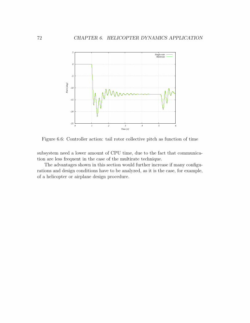
72 CHAPTER 6. HELICOPTER DYNAMICS APPLICATION
-25
-20
-15
-10
-5
0
5
0 1 2 3 4 5 6
Pit
ch [
deg]
Time [s]
Single-rateMultirate
Figure 6.6: Controller action: tail rotor collective pitch as function of time
subsystem need a lower amount of CPU time, due to the fact that communica-tion are less frequent in the case of the multirate technique.
The advantages shown in this section would further increase if many configu-rations and design conditions have to be analyzed, as it is the case, for example,of a helicopter or airplane design procedure.
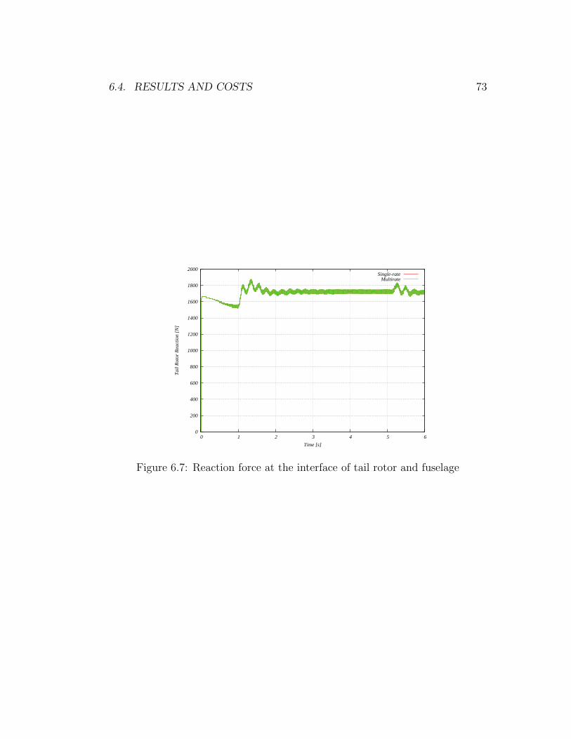
6.4. RESULTS AND COSTS 73
0
200
400
600
800
1000
1200
1400
1600
1800
2000
0 1 2 3 4 5 6
Tai
l Rot
or R
eact
ion
[N]
Time [s]
Single-rateMultirate
Figure 6.7: Reaction force at the interface of tail rotor and fuselage

74 CHAPTER 6. HELICOPTER DYNAMICS APPLICATION

Chapter 7
Conclusions
In this thesis multirate co-simulations have been studied. Performances, in termsof stability and accuracy, have been shown for different numerical methods whichcan be exploited in co-simulation setups.
A new numerical method has been defined, that should improve the com-putational efficiency, especially in parallel simulations. For this method also,stability and accuracy results have been shown, and it possible to conclude thatit exhibits properties similar to the traditional methods.
Only based on free software tools, the co-simulation environment has beenimplemented and tested on a real application.
In conclusion, it has been shown that the multirate co-simulation setup pre-sented in this work show excellent results. Benefits are obtained in both themodel definition procedure and in computational efficiency, two important is-sues related to the simulation of mechanical systems dynamic.
75

76 CHAPTER 7. CONCLUSIONS

Bibliography
[1] W. Schiehlen: Research Trend in Multibody System Dynamics, MultibodySystem Dynamics, 18, 3-13, (2007)
[2] F. Gonzales: Efficient Implementations and Co-simulation Techniques inMultibody System Dynamics, PhD thesis, (Ferrol, March 2010)
[3] M. Busch, M. Arnold, A. Heckmann, and S. Dronka: Interfac-ing SIMPACK to Modelica/Dymola for multidomain vehicle system simu-lations, SIMPACK News, 11, 2, 1-3, (2007)
[4] R. Kubler and W. Schiehlen: Modular simulation in multibody systemdynamics, Multibody System Dynamics, 4, 107127, (2000)
[5] C. W. Gear and D. R. Wells: Multirate Linear Multistep Method, BIT,24, (1984), 484-502.
[6] S. Skelboe: Stability Properties of Backward Differentiation MultirateFormulas, Applied Numerical Math., 5, 151-160, (1989)
[7] A. Verhoeven and E.J.W. Maten: Stability Analysis of the BDF Slow-est first Multirate Methods, International Journal of Computer Mathemat-ics, 84(6), 895-923, (2007)
[8] A. Verhoeven, A. El Guennouni, E.J.W. Maten and R.M.M.
Mattheij: A General Compound Multirate Method for Circuit Simulationproblems, Scientific Computing in Electrical Engineering, ECMI, Vol. 9,143-150, (2006)
[9] F. Gonzales, M. Gonzales and J. Cuadrado: Weak Coupling ofMultibody Dynamics and Block Diagram Simulation Tools, Proceedings ofthe ASME IDETC/CIE 2009, (September 2009, San Diego, California,USA), DETC2009-86653
77

78 BIBLIOGRAPHY
[10] G. Rodriguez: Absolute Stability Analysis of Semi-Implicit Multirate Lin-ear Multistep Methods, (June 2002, Tonanzintla, Puebla)
[11] Quarteroni, Sacco, Saleri: Matematica Numerica, Springer Italia,(2008)
[12] Masarati P, Lanz M, Mantegazza P: Multistep integration of ordi-nary, stiff and differential-algebraic problems for multibody dynamics ap-plications, In XVI Congresso Nazionale AIDAA, pages 71.110, Palermo,September 2428 (2001)
[13] K.A. Stol: Geometry and Structural Properties for the Controls AdvancedResearch Turbine (CART) from Model Tuning, National Renewable EnergyLaboratory, NREL/SR-500-32087, August 25, 2003 November 30, 2003
[14] A. D. Wright and L. J. Fingersh: Advanced Control Design for WindTurbines, NREL/TP-500-42437, (March 2008).
[15] L. Cavagna, A. Fumagalli, P. Masarati, M. Morandini and P.
Mantegazza Real-Time Aeroservoelastic Analysis of Wind-Turbines byFree Multibody Software
[16] www.aero.polimi.it/mbdyn/documentation/examples/
[17] MBDyn Input File Format.
[18] www.gnu.org/licenses/gpl.html
[19] www.fsf.org/about/
[20] www.aero.polimi.it/ mbdyn
[21] www.mathworks.com/products/simulink/
[22] www.ni.com/matrixx/systembuild.htm
[23] www.scicos.org/
[24] www.scicoslab.org/
[25] www.scilab.org/products/xcos